DI

SC

US

SI

ON

P

AP

ER

S

ER

IE

S

Forschungsinstitut zur Zukunft der ArbeitInstitute for the Study of Labor

Polarization and Rising Wage Inequality:Comparing the U.S. and Germany

IZA DP No. 4842

March 2010

Dirk AntonczykThomas DeLeireBernd Fitzenberger

Polarization and Rising Wage Inequality:

Comparing the U.S. and Germany

Dirk Antonczyk University of Freiburg

Thomas DeLeire

University of Wisconsin–Madison, NBER and IZA

Bernd Fitzenberger

University of Freiburg, IFS, ZEW and IZA

Discussion Paper No. 4842 March 2010

IZA

P.O. Box 7240 53072 Bonn

Germany

Phone: +49-228-3894-0 Fax: +49-228-3894-180

E-mail: iza@iza.org

Any opinions expressed here are those of the author(s) and not those of IZA. Research published in this series may include views on policy, but the institute itself takes no institutional policy positions. The Institute for the Study of Labor (IZA) in Bonn is a local and virtual international research center and a place of communication between science, politics and business. IZA is an independent nonprofit organization supported by Deutsche Post Foundation. The center is associated with the University of Bonn and offers a stimulating research environment through its international network, workshops and conferences, data service, project support, research visits and doctoral program. IZA engages in (i) original and internationally competitive research in all fields of labor economics, (ii) development of policy concepts, and (iii) dissemination of research results and concepts to the interested public. IZA Discussion Papers often represent preliminary work and are circulated to encourage discussion. Citation of such a paper should account for its provisional character. A revised version may be available directly from the author.

IZA Discussion Paper No. 4842 March 2010

ABSTRACT

Polarization and Rising Wage Inequality: Comparing the U.S. and Germany*

This paper compares trends in wage inequality in the U.S. and Germany using an approach developed by MaCurdy and Mroz (1995) to separate age, time, and cohort effects. Between 1979 and 2004, wage inequality increased strongly in both the U.S. and Germany but there were various country specific aspects of this increase. For the U.S., we find faster wage growth since the 1990s at the top (80% quantile) and the bottom (20% quantile) compared to the median of the wage distribution, which is evidence for polarization in the U.S. labor market. In contrast, we find little evidence for wage polarization in Germany. Moreover, we see a large role played by cohort effects in Germany, while we find only small cohort effects in the U.S. Employment trends in both countries are consistent with polarization since the 1990s. We conclude that although there is evidence in both the U.S. and Germany which is consistent with a technology-driven polarization of the labor market, the patterns of trends in wage inequality differ strongly enough that technology effects alone cannot explain the empirical findings. JEL Classification: J30, J31 Keywords: wage inequality, polarization, international comparison, cohort study,

quantile regression Corresponding author: Bernd Fitzenberger Department of Economics Albert-Ludwigs-University 79085 Freiburg Germany E-mail: bernd.fitzenberger@vwl.uni-freiburg.de

* We thank David Autor, Thomas E. MaCurdy, Salvador Navarro, Timothy Smeeding, and Christopher Taber for useful discussions. We benefited from valuable comments received at workshops in Berlin and Freiburg. Parts of this paper were written while Dirk Antonczyk was visiting the Institute for Research on Poverty at the University of Wisconsin – Madison. He would like to thank the center for its hospitality. Financial support by the German Research Foundation (DFG) (project “Collective Bargaining and the Distribution of Wages: Theory and Empirical Evidence” in FSP 1169), the German Acadamic Exchange Service (DAAD), and the “Wissenschaftliche Gesellschaft Freiburg” is gratefully acknowledged. The responsibility for all errors is, of course, ours.

Contents

1 Introduction 1

2 Data 6

2.1 CPS for U.S. . . . . . . . . . . . . . . . . . . . . . . . . . . . . . . . . . . 6

2.2 IABS for Germany . . . . . . . . . . . . . . . . . . . . . . . . . . . . . . . 7

2.3 Construction of Cohort-Year-Skill Cells . . . . . . . . . . . . . . . . . . . . 8

3 Basic Empirical Facts 9

3.1 Unconditional Wage Growth . . . . . . . . . . . . . . . . . . . . . . . . . . 9

3.2 Changes in Employment . . . . . . . . . . . . . . . . . . . . . . . . . . . . 11

4 Empirical Approach 11

4.1 Characterization of Wage Profiles . . . . . . . . . . . . . . . . . . . . . . . 12

4.2 Testing for Uniform Wage Growth . . . . . . . . . . . . . . . . . . . . . . 13

4.3 Empirical Implementation . . . . . . . . . . . . . . . . . . . . . . . . . . . 14

5 Results 16

5.1 Estimated Specifications for Wage Equations . . . . . . . . . . . . . . . . . 17

5.2 Life-Cycle Profiles . . . . . . . . . . . . . . . . . . . . . . . . . . . . . . . . 17

5.3 Time-Trends . . . . . . . . . . . . . . . . . . . . . . . . . . . . . . . . . . . 19

5.4 Cohort-effects and Entry Wage Growth . . . . . . . . . . . . . . . . . . . . 20

5.5 Rising Wage Dispersion or Polarization of Wages? . . . . . . . . . . . . . . 21

5.5.1 Development of Skill-Premia due to Macroeconomic-Shifts . . . . . 21

5.5.2 Wage Dispersion within Skill-Groups . . . . . . . . . . . . . . . . . 23

5.5.3 Compositional Effects on Wage growth and Inequality . . . . . . . . 26

5.6 Employment Growth . . . . . . . . . . . . . . . . . . . . . . . . . . . . . . 27

6 Conclusion 28

References 30

Appendix 33

1 Introduction

A substantial body of research has documented increasing wage inequality in industrial-

ized countries. Since the late 1970s and continuing through the mid-2000s, overall wage

inequality has been increasing in the U.S. (e.g. Autor et al., 2008; Lemieux, 2006a), Ger-

many (e.g. Dustmann et al., 2009), the UK (e.g. Machin and Van Reenen, 2008), Canada

(e.g. Boudarbat et al., 2006), and Australia (e.g. Atkinson and Leigh, 2007). As possible

explanations of these trends, most of the literature has focused on skill-biased techno-

logical change (SBTC), the supply of skilled workers, changes in institutions such as the

decline in unionization and changes in the minimum wage, as well as changes in social

norms. SBTC has been the most prominent explanation (see the survey by Katz and

Autor, 1999), which argues that the increase in demand for skills is stronger than the

simultaneous increase in the supply, leading to an increase in wage inequality.

In light of the continuous rise in wage inequality at the top of the wage distribution

in the U.S. and the stagnant or even decreasing wage dispersion at the bottom of the

wage distribution, several recent studies have proposed as a nuanced version of SBTC

that technological change can have a ”polarizing” effect on the labor market rather than

uniformly favoring more skilled groups (e.g. Autor et al., 2003, 2006, 2008; Goos and

Manning, 2007). That is, technological change – for example computerization – can favor

highly skilled groups at the expense of less skilled routine-manual and routine-cognitive

workers and to the advantage of less skilled (non-routine-)manual workers. While labor

market trends seem to be more beneficial for high-skilled jobs relative to medium-skilled

jobs, various studies find a disproportionate growth of employment for low-wage jobs and

a possibly higher wage growth (Autor et al., 2008). Starting in the 1990s, there seems

to be evidence for polarization in employment in the U.S., Germany, and the UK, while

the evidence for polarization of wages is restricted to the U.S. (Goos and Manning, 2007;

Autor et al., 2008; Autor and Dorn, 2009; Dustmann et al., 2009).

The literature has often argued that for SBTC to be a compelling explanation of labor

market trends, the trends have to be similar across different countries having access to the

same technology (Card and Lemieux, 2001). Until the mid-1990s, trends in wage inequal-

ity differed strongly between the U.S. and Germany with increases in wage inequality in

Germany being restricted to the upper part of the wage distribution (Dustmann et al.,

2009; Fitzenberger, 1999). Until the mid-2000s, most of the literature, in fact, assumed

that wage inequality in Germany had been stable since the 1980s and it has been debated

as to whether and to what extent this implies a rejection of the SBTC hypothesis.1 In

light of the polarizing wage trends in the U.S. since the 1990s and in Germany during

1See e.g. Beaudry and Green (2003), Prasad (2004), and Dustmann et al. (2009) as well as thediscussion of the literature in these papers.

1

the 1980s and considering the strong increase in wage inequality across the entire wage

distribution in Germany since the mid-1990s, there are interesting parallels as well as dif-

ferences between the two countries.2 These observations motivate our paper which takes

a fresh look at the comparison of trends in wage inequality in the U.S. and in Germany

using a unified framework of analysis based on comparable data. Furthermore, we account

for potential cohort effects, an issue which is mostly ignored by the recent literature on

wage inequality (see Card and Lemieux (2001) as a notable exception).3 Although SBTC

may have a bias in the age/cohort dimension, most of the recent literature on trends in

wage inequality (see e.g. Autor et al., 2008; Dustmann et al., 2009) restricts itself to a

comparison of cross-sectional age or experience profiles in different years.4

Next, we review the literature in more detail. Autor et al. (2003) first proposed

the task-based polarization hypothesis, focusing on the way technology affects the tasks

performed at a job. Occupations are distinguished by the composition of the different

tasks. Technological change results in a substitution of routine tasks by computers and

other machines. Therefore, demand for workers performing non-routine tasks increases.

For the U.S., Autor et al. (2003) confirm that employment in occupations involving routine

tasks has fallen considerably, whereas employment in high-skilled non-routine jobs in the

upper part of the wage distribution and in non-routine manual jobs in the lower part of the

wage distribution has increased. At about the same time, Manning (2004) and Goos and

Manning (2007) argue that the task-based approach may also rationalize the empirical

fact that the share of low wage jobs involving non-routine tasks with very low skill input

has increased. This is the basis for the polarization hypothesis stating that technological

change may result in a reduction of jobs in the middle of the wage distribution and a

disproportionate growth of both high-wage and low-wage jobs.

Confirming the polarization trend, Autor et al. (2008) provide evidence for a polariza-

2In Germany, the increase in wage inequality in the lower half of the wage distribution began in themid-1990s (Kohn, 2006; Gernandt and Pfeiffer, 2007; Dustmann et al., 2009). Between the early 1980sand the early 1990s, when wage inequality was astonishingly stable in the lower part of the distribution,wage growth at and below the median was substantially higher than in the decade to follow (Dustmannet al., 2009; Fitzenberger, 1999).

3Card and Lemieux (2001) allow for imperfect substitutability between younger and older workers toexplain the fact that the large increase of the wage gap between young college- and high-school graduatesis mainly driven by a slowdown in the growth of college graduates in the U.S. during the 1980s. Theseintercohort shifts in the supply of college graduates occurred while the relative demand for more highlyskilled workers kept increasing steadily. This resulted in a stronger rise of the college-high-school wagegap for younger workers compared to older workers. The authors report similar findings for the UK andCanada. Carneiro and Lee (2008) reanalyze the rising college-high-school premium and provide evidencethat about half of the increase reported may be explained by an increased quality of college graduatesduring this period. This demonstrates that cohort effects may also indicate certain selection processes.

4There exists an earlier literature on wage trends in the 1980s and 1990s which explicitly takes accountof possible cohort effects, see e.g. MaCurdy and Mroz (1995), Card and Lemieux (2001), Gosling et al.(2000), Fitzenberger (1999), Fitzenberger et al. (2001) and Fitzenberger and Wunderlich (2002). Gen-erally, while accounting for the identification problem in the estimation of age, period, and time effects,this literature finds that cohort effects play a role in wage trends.

2

tion of wages in the U.S. during the 1990s such that wage inequality only continued to rise

in the upper part of the wage distribution. Furthermore, Autor and Dorn (2009) find that

employment and wages in low-skill service jobs, which involve non-routine manual tasks

and which pay low wages, have grown considerably since the early 1990s. If technology is

the driving force of labor market developments, we should expect to see similar patterns

in wage growth and polarization in other industrialized countries, provided institutions -

or other developments - do not cause different trends. Even though Goos and Manning

(2007) find evidence for the growth of employment of both low-wage and high-wage jobs

in the UK, they argue that the polarization hypothesis cannot rationalize the finding that

wage inequality did not fall at the bottom of the wage distribution. However, Autor and

Dorn (2009) develop a theoretical model where the wage effects at the bottom of the

wage distribution are ambiguous, because they depend upon whether low-skilled jobs are

complements or substitutes of high-skilled jobs. Thus, technology driven polarization in

employment may also be consistent with rising wage inequality at the bottom of the wage

distribution.

In contrast to technology based explanations for the U.S., DiNardo et al. (1996) and

Lemieux (2006a) argue that increasing wage inequality in the 1980s and the early 1990s

can be explained to an important part by changing labor market institutions, i.e. falling

real minimum wages and deunionization, and changes in the composition of the workforce.

If this were the case, we would not necessarily expect to see similar patterns in wage growth

and polarization in other industrialized countries. Autor et al. (2008) argue that changing

minimum wages and institutions in the U.S. are unlikely to explain the continuing trend

of increasing wage inequality in the upper part of the wage distribution.

Spitz-Oener (2006) confirms the basic findings of Autor et al. (2003) regarding em-

ployment trends in Germany from the late 1970s until the late 1990s. She shows a large

increase both in jobs involving non-routine analytical and interactive tasks, which tend to

be high-wage jobs, and in jobs involving manual tasks, which tend to be low-wage jobs.

In light of these stark changes in employment, it is difficult to rationalize the fairly large

stability in the lower part of the wage distribution in Germany until the mid-1990s.5

All recent studies analyzing wage trends in Germany find increasing wage inequality

at the bottom of the wage distribution (e.g. Kohn, 2006; Gernandt and Pfeiffer, 2007;

Dustmann et al., 2009) since the mid-1990s – a finding that is not inconsistent with the

polarization hypothesis according to Autor and Dorn (2009). Dustmann et al. (2009)

show that occupations at the top of the wage distribution experienced the largest growth

of employment shares and growth of employment shares for occupations in the middle of

the wage distribution appears to be smaller than growth for occupations at the bottom of

5In a recent study on the gender wage gap, Black and Spitz-Oener (2007) confirm polarization inemployment for Germany, which is more pronounced for women compared to men.

3

the wage distribution. They also find a positive statistical relationship between the change

of the share in occupational employment and wage changes above the median, while this

correlation is negative below the median. The authors conclude that the development of

rising wage dispersion in the lower part of the wage distribution is better explained by

episodic changes, e.g. deunionization, than by technological change. The developments

in Germany until the mid-1990s are consistent with the SBTC hypothesis (Fitzenberger,

1999), if one allows for the possibility that growing wage inequality in the lower part

of the wage distribution was prevented by labor market institutions such as unions and

implicit minimum wages implied by the welfare state. Hence, the strong deunionization

(see Dustmann et al., 2009; Fitzenberger et al., 2010) is likely to have contributed to

the increase in inequality at the bottom of the wage distribution since the mid-1990s.

Antonczyk et al. (2009) analyze the changes between 1999 and 2006 in the German wage

structure of male workers and conclude that a task-based approach, based on task data

as used in Spitz-Oener (2006), cannot explain the rise in wage inequality. Gernandt and

Pfeiffer (2007) find that the increase in wage inequality between 1994 and 2005 has been

much stronger for workers with low tenure compared to workers with high tenure. Thus,

new hirings, comprising disproportionately young workers, were affected to a large extent

by the increase in inequality, which could be an indication for cohort effects.

This paper examines trends in wage inequality within and across cohorts of full-time

working men in the U.S. and Germany by describing a set of quantiles. Wage dispersion

in both countries has been rising since the end of the 1970s, as is shown in figure 1 where

cumulated real log wage growth at the median, the 20% quantile, and the 80% quantile

are depicted for male workers for the period from 1979 to 2004. Despite strong evidence

of rising wage inequality in both economies, we find a pattern of wage polarization only

in the United States after 1985 (Autor et al., 2008). Note that our study uses the term

’polarization in wages’ if the ratio of the upper quantile (e.g. the 80% quantile) and the

median increases, while the ratio of the median and the lower quantile (e.g. the 20%

quantile) is stable or even decreases. In Germany, the 80% quantile increases faster than

the 50% quantile, which in turn increases faster than the 20% quantile, while in the U.S.,

the 80% quantile outpaces both the 50% quantile and the 20% quantile. Only until the

mid-1980s, the 20% quantile and the 50% quantile in Germany move in a parallel fashion,

suggesting polarization during the early 1980s. For the U.S., these two lower quantiles

show an almost parallel trend since about 1985. Thus, there has been wage polarization

in the U.S. since 1985 and in Germany prior to 1985.

For our econometric analysis, we use the approach developed by MaCurdy and Mroz

(1995), which allows us to separately identify cohort, age, and macroeconomic effects

on wage profiles. Our main findings can be summarized as follows. We confirm that

between 1979 and 2004, there was, based on conditional time trends, widening wage

4

dispersion in both the U.S. and Germany. This is the case if we consider trends for wages

at the median between skill-groups as well as quantile specific time trends within skill-

groups. However, there are many distinct patterns across the two countries. For example,

for the U.S. we find that time-trends at the median are more positive for high-skilled

workers than for lesser skilled workers throughout the entire period – the medium-low-

skilled gap ceases to increase during the 1990s. Moreover, time-trends within both the

group of low- and medium-skilled workers start polarizing at the end of the 1980s, while

within wage dispersion for high-skilled workers steadily increases. Trends in Germany are

more difficult to interpret. While we find evidence for polarization in Germany across

skill-groups regarding conditional wage trends at the median, we find growing inequality

within the group of low-skilled and median skilled workers after 1985. Moreover, we see a

large role played by cohort effects in Germany – suggesting a role for supply-side effects

or an interaction with institutions in Germany – while we find only small cohort effects

in the U.S..

In addition to wage trends, we analyze the changes in the skill composition of the

workforce and find strong parallel movements between the U.S. and Germany. In both

countries, the decline of the share of low-skilled workers stopped in the mid-1990s and

the mean age of low-skilled workers fell strongly between the 1980s and the late 1990s.

Furthermore, analyzing 10-year changes in employment by age-education cells, we find

in both countries no evidence for polarization of employment in the 1980s and a trend

towards polarization of employment in the late 1990s and early 2000s.

Our results, therefore, are mixed. On the one hand, there is some similar evidence in

wages – and in particular in employment – in the U.S. and Germany which is consistent

with a technology driven polarization of labor market. On the other hand, certain patterns

in wage inequality across the two economies differ strongly enough so that we believe

technology effects alone cannot explain the empirical findings. Episodic changes resulting

from changes in institutional factors such as unionization or the minimum wage may

explain the differences.

The remainder of the paper proceeds as follows: Section 2 describes the two data-sets.

The third section presents the basic facts of wage growth and wage dispersion for the

U.S. and Germany. Section 4 introduces our version of the MaCurdy and Mroz (1995)

approach. The corresponding empirical results are presented in section 5. Finally, section

6 provides our conclusions. The appendix contains graphical illustrations of our estimation

results. Detailed estimation results are available upon request.

5

2 Data

The data we use for our analysis are the U.S. Current Population Survey (CPS) and the

German IAB employment subsample (IABS). We make the two data-sets as comparable

as possible. We concentrate on the group on male workers who are between 25 and 55

years old. This avoids interference with ongoing education and early retirement.

2.1 CPS for U.S.

The U.S. data used for this analysis are from the Current Population Survey, Outgoing

Rotation Groups (CPS-ORG) from 1979-2004. The CPS-ORG data contain wage and

salary information for respondents during the month they levee the basic (monthly) survey.

Wages are inflated to 2004 dollars using the CPI-U-RS. Workers’ calculated hourly wage

rates are either the reported hourly wage (for the 60 percent of workers paid on that basis)

or weekly earnings divided by weekly hours (for the other 40 percent of workers). For

the latter group, earnings per week divided by the usual hours per week was used, unless

information on usual hours per week was missing (in 2004, for example, the figures were

missing for 5 percent of workers not paid on an hourly basis). In that case, the analysis

used the number of actual hours worked in the previous week to construct hourly wages.

While that procedure minimizes the number of workers excluded from the analysis, it

introduces some noise into the calculated hourly rate of pay because the actual hours

worked last week may differ from usual hours worked per week. For roughly 15 percent of

workers not paid on an hourly basis, the number of actual hours worked the previous week

was different from the usual hours per week. Most often, those workers indicated that

they worked part time in the previous week for various reasons, but usually worked full

time. The U.S. Census Bureau imputed data on hourly wage rates, usual weekly earnings,

and usual hours worked per week were used in the analysis. Over the sample period, the

percentage of workers with imputed wage data has increased and was 31 percent in 2004.

We consider male workers from the sample who (normally) work full time. The skill

level between 1979 and 1989 is measured as a categorical variable with three values re-

garding the years of schooling completed:

(U) 12 years or less of schooling (low-skilled)

(M) 13 to 15 years of schooling (medium-skilled)

(H) 16 years or more of schooling (high-skilled).

These categories are defined in a slightly different way after 1990 due to changes in the

CPS: (U) having a high school diploma or less and not having attended college; (M) having

attended college but not having received a degree; and (H) having at least a college degree.

6

Age is measured continuously (in years). Observations are weighted by a person-weight

variable and by the hours worked in the preceding week.

2.2 IABS for Germany

The German data used in the empirical analysis is the IABS (IAB employment subsam-

ple). Although the IABS starts in 1975, we only use data starting from 1979, consistent

with the time period available in the CPS6, and we also inflate wages to 2004 euros. The

IABS involves a randomly drawn 2% sample of employees who participate in the German

Social Security System and is provided by the Institute for Employment Research.7 The

IABS contains about 400,000 individuals in each annual cross-section. This data set or

previous versions of it, have been used to carry out several studies on the German labor

market (e.g. Fitzenberger, 1999; Dustmann et al., 2009).

There are two important advantages of using data from the IABS. First, the IABS is

a very large sample compared to survey data such as the German Socioeconomic Panel,

which is also often used in the analysis of wage trends.8 Second, since individuals are

followed over time, the data set remains representative for the workers contributing to

the social security system. There are three important disadvantages of the IABS. First,

there exists censoring of wages from above. When the daily gross wage exceeds the upper

social security threshold (’Beitragsbemessungsgrenze’), the daily social security threshold

is reported instead. This censoring affects roughly the top 10%-14% of the workers in the

wage distribution.9 Among university graduates, censoring from above can affect about

half of the population. This is one of the reasons why we estimate quantile regressions

of wages, which are robust against this kind of right censoring.10 Second, there exists a

structural break in 1984. Since that year, one-time payments and other bonuses have been

included in the reported earnings leading to an increase in the observed inequality of wages

at that time. The technique employed by Fitzenberger (1999) is used as a conservative

correction.11 Third, the IABS does not provide detailed information on hours worked,

6Between 1975 and 1979, a slight increase of wage dispersion in the upper part of the distributiontakes place and virtually no change in wage-dispersion in the lower part, as measured by the 80%-50%and 50%-20% difference of log-wages.

7It is mandatory for every employee in Germany to adhere to the German social security, given heworks regularly and his wage passes a certain earnings threshold. Civil servants are the largest groupof workers that do not participate in the German Social Security system. Taken into accounts furtherexceptions (e.g. students), about 80% of the German employees are covered.

8Gernandt and Pfeiffer (2007) provide an overview of the data-sets used in recent studies regardingwage dispersion in Germany.

9The value of this threshold changes annually.10There exists also truncation from below in the IABS: If the wage lies below the lower social security

threshold, the employee is not obliged to pay social security contribution and is thus excluded. As weconcentrate on full-time working males, this restriction is negligible.

11See also Fitzenberger and Wunderlich (2002) and Dustmann et al. (2009) for similar correctionprocedures.

7

but it provides an indicator for full-time work. As we restrict the analysis to full-time

working males, our results are likely to be robust and comparable to the U.S.-data.12

Workers are grouped by their skills according to the following formal education levels

given in the IABS:

(U) without a vocational training degree (low-skilled)

(M) with a vocational training degree (medium-skilled)

(H) with a technical college (”Fachhochschule”) or a university degree (high-skilled)

2.3 Construction of Cohort-Year-Skill Cells

Our level of analysis are wage quantiles by year, cohort/age, and skill level, where cohort

is defined by year of birth. For each cell, we calculate different quantiles for the real wage.

Applying the approach proposed by Fitzenberger (1999), this is done for the German data

in the following way. The IABS contains information on the social security insurance spells

comprising the starting point and the end point as well as the average daily gross wage13

(excluding employer’s distribution) for this spell.

An annual wage observation for one individual is calculated as the weighted average

of the wages he earned during his different spells within one year, where the spell lengths

are used as the weights. The sum of the spell lengths for all individuals in one cell is used

to calculate the number of employed workers within this cell. This variable is used as a

weight in the regressions.

The next step consists of calculating the 20%, 50%, and 80% quantile for the cells,

where again the spell lengths are used as weights. We also record the sum of spell lengths

as cell weights. In the case of Germany, when the quantile coincides with the threshold, it

is recorded as being censored. These information are sufficient for our empirical analysis

to estimate quantile regressions based on cell data. The cohort-year-skill cell data for

the CPS are constructed in an analogous way as for the German data, using the weights

described above.

12Trends in wage inequality among German full-time-working males are robust to either taking hourlywages (provided e.g. in the German Socioeconomic Panel) or taking monthly wages (for details see e.g.Dustmann et al., 2009).

13The daily social security threshold is reported instead if the daily gross wage exceeds the upper socialsecurity threshold, see above.

8

3 Basic Empirical Facts

3.1 Unconditional Wage Growth

Figure 1 depicts the unconditional wage growth jointly for all skill-groups between 1979

and 2004. For the U.S., wages at the three quantiles fall until 1996, with the largest

decline at the 20% quantile being -13 log percentage points (pp). Wages at the median

decline 10 log pp and those at the 80% quantile decline 4 log pp. This implies rising wage

dispersion both in the upper and the lower part of the U.S. wage distribution. Between

1996 and 2004, wages grow at all quantiles, whereby wages at the 20% quantile and at

the 80% quantile rise about 9 log pp, which is 1-2 log pp more than the rise of the wages

at the median. This widening of the wage distribution at the top and narrowing at the

bottom provides evidence of polarization of wages during the 1996 to 2004 period. Overall,

however, between 1979 and 2004 the dispersion both in the upper half of the distribution

(as measured by 80-50 log difference) and in the bottom half (as measured by the 50-20

log difference) increased.

For Germany, wages throughout the distribution start to grow in the mid-1980s, and

wages at the 80% quantile exhibit larger growth rates than those at the median and the

20% quantile. Wage inequality in the upper part of the wage distribution keeps rising

steadily since the beginning of the 1980s, while wage dispersion in the lower part of the

wage distribution only starts to increase in the mid-1990s. These results are in line with

Dustmann et al. (2009).14 Between 1979 and 2004, the 20% quantile, the median, and

the 80% quantile increase by 9, 15, and 20 log pp, respectively – cumulative real wage

growth between 1979 and 2004 is considerably higher in Germany compared to the U.S..

Finally, in Germany, the 20% quantile and the 80% quantile only grow both faster than

the median during the early 1980s – thus a polarization of wages can be observed only

for a short period of time.

Turning to skill-group specific trends, figure 2 shows the unconditional cross-sectional

wage growth at different quantiles conditional on education and figure 3 summarizes

overall wage dispersion (as measured by the 80-20 difference of log-wages), as well as

dispersion in the lower and the upper part of the skill-specific wage distributions (as

measured by the 50-20 and 80-50 differences, respectively).

Between 1979 and 1996 low-skilled workers in the U.S. lost about 32 to 34 log pp in

terms of real wages. At the same time, the sharpest decline of wage inequality in the lower

part of the distribution occurred among this group. Wages at the 20% quantile gained

12 log pp during the eight following years. Workers at the median and the 80% quantile

were also able to recover, but that recovery was less pronounced for these groups. The

14Note that Dustmann et al. (2009) use the 85% quantile and the 15% quantile.

9

80-50 difference stays rather stable over time, while the 50-20 difference starts to decline

at the beginning of the 1990s. Wages of medium-skilled workers also increased after a

low in 1996 and a clear pattern of polarization is observable since the early 1990s, as

the 80-50 difference keeps increasing and the 50-20 difference starts to decrease. In the

U.S., only the group of high-skilled workers has higher real wages in 2004 than in 1979.

Although only wages at the lowest quantile incurred real wage losses between 1979 and

1996 among this group, wage inequality in both parts of the distribution is slightly but

steadily increasing since the late 1980s. Similar observations regarding the development

of the wage structure have been made by e.g. Autor et al. (2006).

In Germany, only low-skilled workers at the 20% quantile had lower real wages in 2004

than in 1979 (a 10 log pp cumulative decline). This wage-loss stems from a period of

sharp decline beginning in the early 1990s. During the last twelve years of observation,

the 20% quantile of wages fell by 20 log pp. Wages at the median also fell, but to

a lesser degree, while trends at the 80% quantile have been flat since the early 1990s.

Up until 1991/92, wages moved quite uniformly along the entire wage distribution. In

1992/93 a severe recession took place in Germany and since then, wage dispersion has

been increasing in the lower as well in the upper part of the distribution.15 Medium-

skilled workers in Germany, making up the major part of the entire German workforce,

experience quite similar movements as described above for the overall wage distribution

not conditioning on educational-level – rising wage dispersion in the upper part beginning

in the 1980s and increasing wage inequality in the lower part of the distribution since the

mid-1990s. Furthermore, similar to the development of the entire wage-distribution, we

observe a polarizing pattern of wages until 1984. German high-skilled workers experience

considerable gains since the early 1980s: wages rose by 17 log pp and 30 log pp for workers

at the 20% quantile and the median respectively, resulting in an increasing dispersion in

the lower part of the conditional distribution of wages.

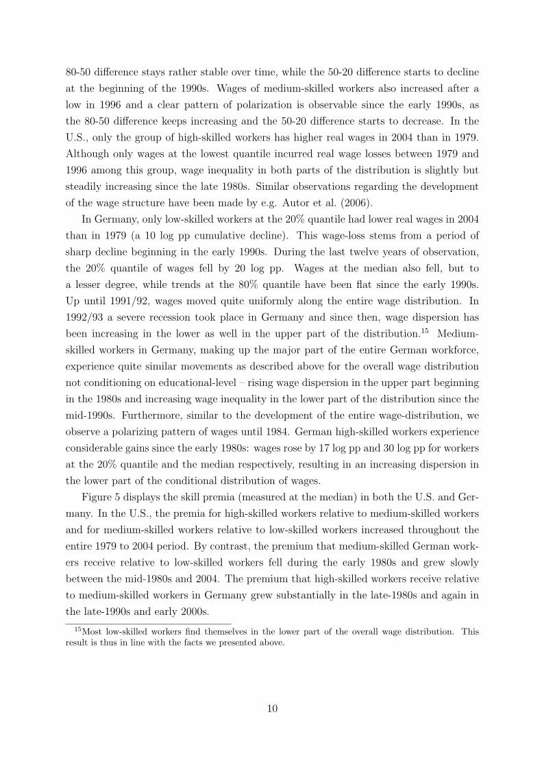
Figure 5 displays the skill premia (measured at the median) in both the U.S. and Ger-

many. In the U.S., the premia for high-skilled workers relative to medium-skilled workers

and for medium-skilled workers relative to low-skilled workers increased throughout the

entire 1979 to 2004 period. By contrast, the premium that medium-skilled German work-

ers receive relative to low-skilled workers fell during the early 1980s and grew slowly

between the mid-1980s and 2004. The premium that high-skilled workers receive relative

to medium-skilled workers in Germany grew substantially in the late-1980s and again in

the late-1990s and early 2000s.

15Most low-skilled workers find themselves in the lower part of the overall wage distribution. Thisresult is thus in line with the facts we presented above.

10

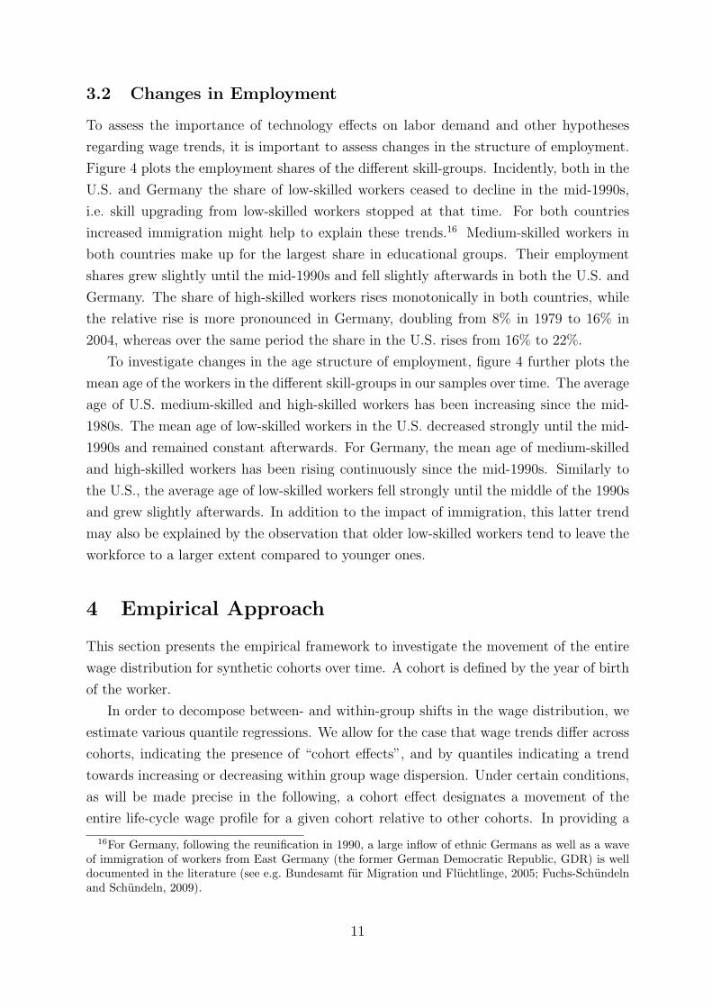
3.2 Changes in Employment

To assess the importance of technology effects on labor demand and other hypotheses

regarding wage trends, it is important to assess changes in the structure of employment.

Figure 4 plots the employment shares of the different skill-groups. Incidently, both in the

U.S. and Germany the share of low-skilled workers ceased to decline in the mid-1990s,

i.e. skill upgrading from low-skilled workers stopped at that time. For both countries

increased immigration might help to explain these trends.16 Medium-skilled workers in

both countries make up for the largest share in educational groups. Their employment

shares grew slightly until the mid-1990s and fell slightly afterwards in both the U.S. and

Germany. The share of high-skilled workers rises monotonically in both countries, while

the relative rise is more pronounced in Germany, doubling from 8% in 1979 to 16% in

2004, whereas over the same period the share in the U.S. rises from 16% to 22%.

To investigate changes in the age structure of employment, figure 4 further plots the

mean age of the workers in the different skill-groups in our samples over time. The average

age of U.S. medium-skilled and high-skilled workers has been increasing since the mid-

1980s. The mean age of low-skilled workers in the U.S. decreased strongly until the mid-

1990s and remained constant afterwards. For Germany, the mean age of medium-skilled

and high-skilled workers has been rising continuously since the mid-1990s. Similarly to

the U.S., the average age of low-skilled workers fell strongly until the middle of the 1990s

and grew slightly afterwards. In addition to the impact of immigration, this latter trend

may also be explained by the observation that older low-skilled workers tend to leave the

workforce to a larger extent compared to younger ones.

4 Empirical Approach

This section presents the empirical framework to investigate the movement of the entire

wage distribution for synthetic cohorts over time. A cohort is defined by the year of birth

of the worker.

In order to decompose between- and within-group shifts in the wage distribution, we

estimate various quantile regressions. We allow for the case that wage trends differ across

cohorts, indicating the presence of “cohort effects”, and by quantiles indicating a trend

towards increasing or decreasing within group wage dispersion. Under certain conditions,

as will be made precise in the following, a cohort effect designates a movement of the

entire life-cycle wage profile for a given cohort relative to other cohorts. In providing a

16For Germany, following the reunification in 1990, a large inflow of ethnic Germans as well as a waveof immigration of workers from East Germany (the former German Democratic Republic, GDR) is welldocumented in the literature (see e.g. Bundesamt fur Migration und Fluchtlinge, 2005; Fuchs-Schundelnand Schundeln, 2009).

11

parsimonious representation of trends in the entire wage distribution, we are able to pin

down precisely the differences in wage trends across groups of workers defined by skill

level. In light of the descriptive evidence presented in the previous section, we explicitly

take into account the possibility that wage differences are sensitive to the business cycle as

well as the possibility that they differ by age and by the position in the wage distribution.

Due to the inherent identification problem between age, cohort, and time effects on

wages, wage profiles based on cross-section relationships between age and wages over a

sequence of years and movements of life-cycle wage profiles faced by successive cohorts are

statistically indistinguishable. However, considering the wage growth experienced by a

particular cohort over time or over age, it can be tested whether apart from the differential

age effect, different cohorts exhibit the same time trend. We use the approach developed

by MaCurdy and Mroz (1995), which has also been applied by Fitzenberger et al. (2001)

and Fitzenberger and Wunderlich (2002) for West Germany and by Gosling et al. (2000)

for the UK. For details, see MaCurdy and Mroz (1995) and Fitzenberger and Wunderlich

(2002).

4.1 Characterization of Wage Profiles

We denote the age of an employee by α and calendar time by t. A cohort c can be defined

by the year of birth. The variables age, cohort and calendar year are linked by the relation

t = c+ α. Studies of wage trends often investigate movements of “age-earnings profiles”

(1) ln[w(t, α)] = f(t, α) + u .

The deterministic function f measures the systematic variation in wages and u reflects

cyclical or transitory phenomena. For a fixed year t, the function f(t, α) yields the

conventional cross-sectional wage profiles. Movements of f as a function of t describe how

cross-sectional wage profiles shift over time. The cross-sectional relation f as a function

of age does not describe “life-cycle” wage growth for any cohort or, put differently, the

cross-sectional relation may very well be the result of “cohort effects”. In fact, “cohort-

earnings profiles” are statistically indistinguishable from “age-earnings profiles”. Wage

profiles can also be expressed as a function of cohort and age

(2) g(c, α) ≡ g(t− α, α) ≡ f(t, α)

where the deterministic function g describes how age-earnings profiles differ across cohorts.

Holding age constant, g(c, α) describes the profiles of wages earned by different cohorts

over time. Holding the cohort constant yields the profile experienced by a specific cohort

over time and age. The latter is referred to as the “life-cycle profile”, because it reflects

12

the wage movements over the life-cycle of a given cohort.

The different parameterizations g(c, α) and f(t, α) are equivalent representations of

the same wage profile. Without further assumptions, “pure life-cycle effects” due to aging

or “pure cohort effects” cannot be identified. We focus on wage trends for a given cohort.

4.2 Testing for Uniform Wage Growth

Our analysis by skill-group investigates whether wage trends are uniform across cohorts

in the sense that every cohort experiences the same time trend in wages and the same

age-specific wage growth (life-cycle effect). Despite the identification issues discussed

above, the existence of a uniform time trend across cohorts is a testable implication in

the framework presented here. If such a uniform time trend is found, it is designated as

the macroeconomic wage trend for the group of workers considered.

One notion of wage growth proves useful: Wage growth for a given cohort in the labor

market over time (“Insider Wage Growth”), given by

(3)∂g

∂t|c =

∂g

∂α|c ≡ gα(c, α) ≡ gα,

comprising the simultaneous change of time and age. Alternatively, holding age constant

yields the change of wages earned by different cohorts at specific ages. For the age at

labor market entry, αe, entry wage growth is given by

(4)∂g

∂t|α=αe =

∂g

∂c|α=αe ≡ gc(c, αe) = gc(t− αe, αe) ≡ e(t) ,

again comprising two effects, namely a change of cohort and time.

If wage growth can be characterized as the sum of a pure aging effect and a pure time

effect in the following way

(5) gα = a(α) + b(t) = a(α) + b(c+ α),

then life-cycle wage growth a(α) is independent of the calendar year t. This condition is

designated as the “uniform insider wage growth hypothesis”. If condition (5) holds, we can

construct a “life-cycle wage profile” independent of the calendar year and a macroeconomic

time trend independent of age. We test condition (5) by testing for the significance of

interaction terms of α and t in the specification of gα.

Integrating back condition (5) on the derivative gα with respect to α yields an additive

form for the systematic component of the wage function g(c, α):

(6) g(c, α) = G+K(c) + A(α) +B(c+ α)

13

where G +K(c) is the cohort specific constant of integration. At a given point in time,

the wages of cohorts differ only by the age-effect, given by A(α), and by a cohort-specific

level, given by K(c). The “uniform insider wage growth hypothesis” HUI can be tested

by investigating whether “interaction terms” R(α, t) enter specification (6) which are

constructed as integrals of interaction terms of α and t in gα.

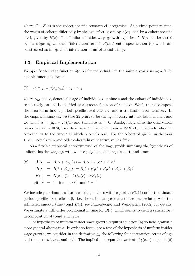
4.3 Empirical Implementation

We specify the wage function g(c, α) for individual i in the sample year t using a fairly

flexible functional form:

(7) ln[wi,t] = g(ci, αi,t) + ut + ui,t

where αi,t and ci denote the age of individual i at time t and the cohort of individual i,

respectively. g(c, α) is specified as a smooth function of c and α. We further decompose

the error term into a period specific fixed effect ut and a stochastic error term uit. In

the empirical analysis, we take 25 years to be the age of entry into the labor market and

we define α = (age − 25)/10 and therefore αe = 0. Analogously, since the observation

period starts in 1979, we define time t = (calendar year − 1979)/10. For each cohort, c

corresponds to the time t at which α equals zero. For the cohort of age 25 in the year

1979, c equals zero and older cohorts have negative values for c.

As a flexible empirical approximation of the wage profile imposing the hypothesis of

uniform insider wage growth, we use polynomials in age, cohort, and time:

A(α) = A1α+ A(2)(α) = A1α+ A2α2 + A3α

3(8)

B(t) = B1t+B(2)(t) = B1t+B2t2 +B3t

3 +B4t4 +B5t

5

K(c) = K1c+ (1− δ)Kb(c) + δKa(c)

with δ = 1 for c ≥ 0 and δ = 0 .

We include year dummies that are orthogonalized with respect to B(t) in order to estimate

period specific fixed effects ut, i.e. the estimated year effects are uncorrelated with the

estimated smooth time trend B(t), see Fitzenberger and Wunderlich (2002) for details.

We estimate a fifth order polynomial in time for B(t), which seems to yield a satisfactory

decomposition of trend and cycle.

The hypothesis of uniform insider wage growth requires equation (6) to hold against a

more general alternative. In order to formulate a test of the hypothesis of uniform insider

wage growth, we consider in the derivative gα the following four interaction terms of age

and time αt, αt2, α2t, and α2t2. The implied non-separable variant of g(c, α) expands (6)

14

by incorporating the integrals of these interaction terms, denoted by R1-R4, see MaCurdy

and Mroz (1995) and Fitzenberger and Wunderlich (2002) for details, and we test for

significance of R1-R4.

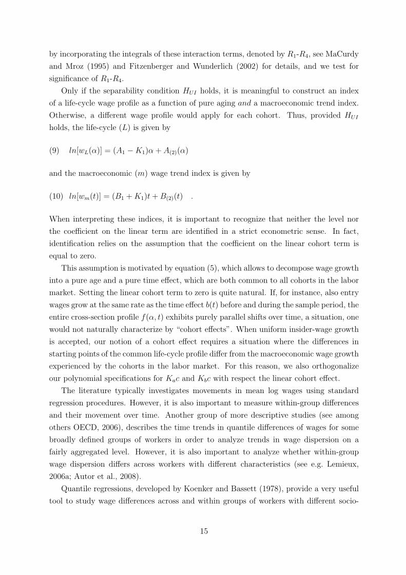
Only if the separability condition HUI holds, it is meaningful to construct an index

of a life-cycle wage profile as a function of pure aging and a macroeconomic trend index.

Otherwise, a different wage profile would apply for each cohort. Thus, provided HUI

holds, the life-cycle (L) is given by

(9) ln[wL(α)] = (A1 −K1)α+ A(2)(α)

and the macroeconomic (m) wage trend index is given by

(10) ln[wm(t)] = (B1 +K1)t+B(2)(t) .

When interpreting these indices, it is important to recognize that neither the level nor

the coefficient on the linear term are identified in a strict econometric sense. In fact,

identification relies on the assumption that the coefficient on the linear cohort term is

equal to zero.

This assumption is motivated by equation (5), which allows to decompose wage growth

into a pure age and a pure time effect, which are both common to all cohorts in the labor

market. Setting the linear cohort term to zero is quite natural. If, for instance, also entry

wages grow at the same rate as the time effect b(t) before and during the sample period, the

entire cross-section profile f(α, t) exhibits purely parallel shifts over time, a situation, one

would not naturally characterize by “cohort effects”. When uniform insider-wage growth

is accepted, our notion of a cohort effect requires a situation where the differences in

starting points of the common life-cycle profile differ from the macroeconomic wage growth

experienced by the cohorts in the labor market. For this reason, we also orthogonalize

our polynomial specifications for Kac and Kbc with respect the linear cohort effect.

The literature typically investigates movements in mean log wages using standard

regression procedures. However, it is also important to measure within-group differences

and their movement over time. Another group of more descriptive studies (see among

others OECD, 2006), describes the time trends in quantile differences of wages for some

broadly defined groups of workers in order to analyze trends in wage dispersion on a

fairly aggregated level. However, it is also important to analyze whether within-group

wage dispersion differs across workers with different characteristics (see e.g. Lemieux,

2006a; Autor et al., 2008).

Quantile regressions, developed by Koenker and Bassett (1978), provide a very useful

tool to study wage differences across and within groups of workers with different socio-

15

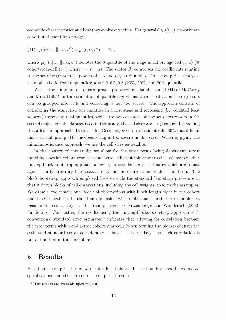
economic characteristics and how they evolve over time. For general θ ∈ (0, 1), we estimate

conditional quantiles of wages

(11) qθ(ln[wi,t]|c, α, βθ) = gθ(c, α, βθ) + uθt ,

where qθ,t(ln[wi,t]|c, α, βθ) denotes the θ-quantile of the wage in cohort-age-cell (c, α) (≡cohort-year-cell (c, t) where t = c + α). The vector βθ comprises the coefficients relating

to the set of regressors (≡ powers of c, α and t; year dummies). In the empirical analysis,

we model the following quantiles: θ = 0.2, 0.5, 0.8 (20%, 50%, and 80% quantile).

We use the minimum-distance approach proposed by Chamberlain (1994) or MaCurdy

and Mroz (1995) for the estimation of quantile regressions when the data on the regressors

can be grouped into cells and censoring is not too severe. The approach consists of

calculating the respective cell quantiles in a first stage and regressing (by weighted least

squares) those empirical quantiles, which are not censored, on the set of regressors in the

second stage. For the dataset used in this study, the cell sizes are large enough for making

this a fruitful approach. However, for Germany, we do not estimate the 80% quantile for

males in skill-group (H) since censoring is too severe in this case. When applying the

minimum-distance approach, we use the cell sizes as weights.

In the context of this study, we allow for the error terms being dependent across

individuals within cohort-year-cells and across adjacent cohort-year-cells. We use a flexible

moving block bootstrap approach allowing for standard error estimates which are robust

against fairly arbitrary heteroscedasticity and autocorrelation of the error term. The

block bootstrap approach employed here extends the standard bootstrap procedure in

that it draws blocks of cell observations, including the cell weights, to form the resamples.

We draw a two-dimensional block of observations with block length eight in the cohort

and block length six in the time dimension with replacement until the resample has

become at least as large as the resample size, see Fitzenberger and Wunderlich (2002)

for details. Contrasting the results using the moving-blocks-bootstrap approach with

conventional standard error estimates17 indicates that allowing for correlation between

the error terms within and across cohort-year-cells (when forming the blocks) changes the

estimated standard errors considerably. Thus, it is very likely that such correlation is

present and important for inference.

5 Results

Based on the empirical framework introduced above, this section discusses the estimated

specifications and then presents the empirical results.

17The results are available upon request.

16

5.1 Estimated Specifications for Wage Equations

We estimate two specifications for the 20%, 50%, and 80% quantile for males by skill-

groups (U), (M), and (H). The high degree of censoring allows only estimation for the

20% and the 50% quantile in the case of high-skilled (H) males in Germany. The more

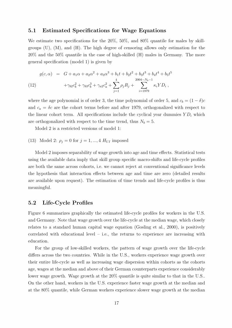
general specification (model 1) is given by

g(c, α) = G+ a1α+ a2α2 + a3α

3 + b1t+ b2t2 + b3t

3 + b4t4 + b5t

5

+γb2c2b + γb3c

3b + γa2c

2a +

4∑j=1

ρjRj +

2004−Nb−1∑i=1979

κiY Di ,(12)

where the age polynomial is of order 3, the time polynomial of order 5, and cb = (1− δ)c

and ca = δc are the cohort terms before and after 1979, orthogonalized with respect to

the linear cohort term. All specifications include the cyclical year dummies Y Di which

are orthogonalized with respect to the time trend, thus Nb = 5.

Model 2 is a restricted versions of model 1:

Model 2: ρj = 0 for j = 1, ..., 4 HUI imposed(13)

Model 2 imposes separability of wage growth into age and time effects. Statistical tests

using the available data imply that skill group specific macro-shifts and life-cycle profiles

are both the same across cohorts, i.e. we cannot reject at conventional significance levels

the hypothesis that interaction effects between age and time are zero (detailed results

are available upon request). The estimation of time trends and life-cycle profiles is thus

meaningful.

5.2 Life-Cycle Profiles

Figure 6 summarizes graphically the estimated life-cycle profiles for workers in the U.S.

and Germany. Note that wage growth over the life-cycle at the median wage, which closely

relates to a standard human capital wage equation (Gosling et al., 2000), is positively

correlated with educational level – i.e., the returns to experience are increasing with

education.

For the group of low-skilled workers, the pattern of wage growth over the life-cycle

differs across the two countries. While in the U.S., workers experience wage growth over

their entire life-cycle as well as increasing wage dispersion within cohorts as the cohorts

age, wages at the median and above of their German counterparts experience considerably

lower wage growth. Wage growth at the 20% quantile is quite similar to that in the U.S..

On the other hand, workers in the U.S. experience faster wage growth at the median and

at the 80% quantile, while German workers experience slower wage growth at the median

17

and the 80% quantile, leading to a decreasing within-cohort wage dispersion in Germany,

but rising within-cohort wage dispersion in the U.S..

What are possible causes of these cross-national differences? The decreasing within-

cohort wage dispersion over time for German low-skilled workers may be due to a selection-

process. Older German low-skilled workers at the bottom of the skill-specific wage distri-

bution might drop out of the labor-market as they get older, e.g. due to layoffs, if their

productivity lies below the wages set by union wage agreements. Another reason might be

that U.S. low-skilled workers are more heterogeneous than German low-skilled workers, as

in the U.S. on-the-job training or internal education after entering the workforce is more

widespread among low-skilled workers than it is in Germany, where the educational and

training systems tend to be more formal.

For the U.S., the group of medium-skilled workers is defined as those who finished

high-school and those who subsequently received between one and three years of college

education – 55% to 60% of the U.S. workforce falls within this category. Medium-skilled

workers in Germany are the largest group of employees, making up 75% to 80% of the

workforce. Workers in this group typically receive vocational training after finishing

between nine and ten years of secondary schooling, resulting in a total of twelve to thirteen

years of formal education. Interestingly, for the U.S., wages at and above the median

change quite similarly, exhibiting cumulated growth over the life-cycle of about 40 log

pp, just as wages at the 80% quantile in Germany do. Wages at the median in Germany

rise only about 28 log pp though. At the lower end of the distribution in the U.S.

workers experience higher cumulated wage growth (32 log pp) over their life-cycle as well,

compared to their German counterparts (23 log pp). Thus, contrary to the low-skilled,

the increase of within-cohort wage dispersion associated with aging is twice as strong for

German medium-skilled workers compared to U.S. medium-skilled workers.

For the group of high-skilled workers in the U.S., wages increase 48, 55, and 56 log pp

over the life-cycle at the 20%, 50%, and 80% quantile, respectively – resulting once again

in an increasing within-cohort wage dispersion for this skill-group. Recall, that due to

censoring in the German data, we restrict ourselves to the 20% quantile and the median

for the group of high-skilled workers in Germany. Life-cycle wage growth for workers at

the 20% quantile results in a cumulated gain of 56 log pp over the life-cycle. Examining

the life-cycle profile at the median wage for high-skilled workers based on the conditional

quantile models described above shows stronger life-cycle wage growth than for other

skill-groups, resulting in a cumulated gain of 55-60 log pp over the life-cycle. The increase

until age 50 is about 10 log pp higher at the median compared to the 20% quantile.

The results regarding the development of wage dispersion over the life-cycle for the U.S.

are in line with findings for the UK (Gosling et al., 2000). The growth of wage dispersion

over the life-cycle conditional on education is negatively correlated with skill level, i.e. in

18

the U.S. low-skilled workers experience the highest increase in wage dispersion over the

life-cycle, while for Germany dispersion increases most strongly for medium-skilled in the

upper part of the wage distribution.

5.3 Time-Trends

Figure 7 depicts trends in real wages due to macroeconomic-shifts in the U.S. and Ger-

many. The macroeconomic-shifts affect all cohorts uniformly within the same skill-group

at the same point in time (but at different points in their life-cycle). These macro-shifts

are purged of cohort effects and of life-cycle effects. At first glance we see that time-trends

in the U.S. were more positive for workers with higher educational attainment than for

low- and medium-skilled workers. Comparing low- and medium-skilled workers in Ger-

many at the different quantiles, we see that time-trends in wages were roughly the same

across skill-groups. Time-trends for German high-skilled workers were similar to those

of less skilled workers until the early 1990s, but wage growth was stronger thereafter.

Finally, our estimates suggest that time-trends in wages developed more positively for

German workers than for U.S. workers.

The mid-1990s mark a turning point in the development of the macro wage indices of

both low-skilled and medium-skilled worker in the U.S.. Until that point in time, workers

in both subgroups experienced real wage losses throughout the entire wage distribution,

being stronger for the low-skilled (-30 log pp at the 80% and 20% quantile and -32 log pp

at the median). Medium-skilled workers incurred losses of -11, -20, and -22 log pp with at

the 80%, 50%, and 20% quantile, respectively. Between 1996 and 2004, however, wages

grew considerably at all considered quantiles of both low- and medium-skilled workers.

Wages of the low-skilled at the 20% quantile grew about 10 log pp, wages at the median

and at the 80% quantile experienced a gain of 5 log pp. In the group of the medium-

skilled, the wage growth starting in the mid-1990s was less pronounced. Wage growth

was about 4 log pp at both the 20% and the 80% quantile and about 3 log pp at the

median. Time-trends are most positive for the group of high-skilled workers in the U.S.,

with a cumulated wage growth of -1, 8, and 17 log pp at the 20%, 50%, and 80% quantile,

respectively, between 1979 and 2004.

For low-skilled workers in Germany, the 20%, 50%, and 80% quantiles of the wage

distribution move in a parallel manner between 1979 and 1992, resulting in an uniform

gain of about 8 log pp along the entire distribution. Thereafter, wages at the 80% quantile

exhibit small gains, while the wages at the 20% quantile decrease, resulting in real wage

losses of 5 log pp between 1992 and 2004. Wages at the median remain flat during this

period.18. Medium-skilled workers in Germany do slightly better than low-skilled workers,

18One possible cause for the declines in wages among low-skilled workers at the lower end of this wage

19

in terms of time-trends at the lower end of the skill-specific wage-distribution. Time-trends

for wages at and above the median are fairly similar. Cumulated wage growth at the 20%

quantile for German medium-skilled workers is slightly above zero, compared to real wage

losses of about 2 log pp in the group of the low-skilled. However, this masks the fact that

since the beginning of the 1990s, real wage losses are more pronounced among low-skilled

workers in the lower part of the distribution. Wages at the 20% quantile of German high-

skilled workers were staying flat since the beginning of the 1990s. Over the entire period,

cumulated wage growth is about 1 log pp for this group at the 20% quantile. The time-

trend for German high-skilled workers at the median starts to increase monotonically in

the early 1980s, at an annual rate of about 0.5 log pp. Wages at the 20% quantile were

rising between the early 1980s and the early 1990s, but then started to flatten out.

5.4 Cohort-effects and Entry Wage Growth

Cohort-effects can occur for at least two reasons. The first relates to supply-side effects,

as discussed by Card and Lemieux (2001), who argue that the increasing wage-premium

between college graduates and high-school graduates is due to a slowdown in the growth

of supply of higher-skilled workers. The second is an interaction between tenure and

wage dispersion, as put forward by Gernandt and Pfeiffer (2007), who find that wage

dispersion was rising most strongly among workers with low tenure in Germany.19 In

addition, cohort effects may be implied by wage adjustments which are strongest among

younger workers and which persist over the life cycle. These interpretations are not

necessarily contradictory.

Figure 8 plots the estimated cohort effects for the different groups in both economies.

These are quadratic and cubic terms for cohorts that enter the labor market before and

after 1979, orthogonalized to the linear cohort term. For both medium- and high-skilled

workers in the U.S., negative cohort effects are estimated for the oldest cohorts and

positive effects for the youngest cohorts. For low-skilled workers, we find positive cohort-

effects for the youngest cohorts and negative ones for the oldest cohorts at the 80%

quantile. Interestingly, we find that during the 1980s cohort-effects had a positive effect on

medium-skilled and high-skilled workers – this is the period for which Card and Lemieux

(2001) observed increasing skill-premia among younger workers for the U.S..20

distribution (and therefore at the lower end in the overall wage distribution) may be the large inflow(immigration) of low-skilled workers into West-Germany after the reunification, resulting in an highersupply of low-skilled workers, in combination with the recession that took place in Germany in 1992/93,see section 3

19Changes in educational policy, or more generally, any pre-labor market conditions, may also becaptured by cohort-effects in our specification.

20Increasing wage dispersion due to cohort effects across skill-groups may also indicate selection effects,i.e. the ”ability” of workers within skill-groups can change over time, see section 1.

20

For Germany, for all skill-groups, both the youngest and the oldest cohorts exhibit

negative cohort-effects, relative to the cohorts entering the labor market between the

mid-1960s and mid-1980.21 Furthermore, the youngest cohorts experience higher within-

cohort wage dispersion due to these effects.

Cohort effects and time-trends additively define entry wage growth. To see the inter-

action between the macroeconomic-shifts and the cohort-specific effects, figure 9 plots the

development of entry wages conditional on educational achievement. During 1979 and

2004 entry-wages in the U.S. become more dispersed among medium- and high-skilled

workers, and less dispersed for U.S. low-skilled workers. However, the decline of entry

wages for the latter group is severe throughout the skill specific distribution. Entry wages

decline for medium-skilled workers, while they rise for high-skilled U.S. workers. The

overall within skill-group wage dispersion increases by 10 log pp for the medium-skilled

and 15 log pp for the high-skilled. The difference between the medians across skill-groups

increases by 22 log pp. However, this is primarily due to time-effects across skill-groups.

Cohort-effects across skill-groups seem to play a minor role.

Entry wages for German workers across skill-groups begin to disperse in the early

1990s. Strong negative cohort effects – being larger in size for the lesser skilled workers

– for the youngest cohorts complement the dispersion stemming from the time-trends.

For low- and medium-skilled workers, wages at the median in 2004 lie below their level

from 1979, whereby losses are more pronounced for low-skilled workers at all observed

quantiles. Furthermore, wage dispersion among low-skilled workers is more pronounced

than for medium-skilled workers. Entry-wages of high-skilled workers at the median are

about 10 log pp higher in 2004 than in 1979, while the difference to wages at the 20%

quantile in this group increased by 20 log pp.

5.5 Rising Wage Dispersion or Polarization of Wages?

5.5.1 Development of Skill-Premia due to Macroeconomic-Shifts

How much of the increase in wage dispersion in the U.S. and Germany is due to rising

skill-premia across educational groups? Some studies have suggested that this part is

substantial. For example Lemieux (2006b) finds that almost half of the increase in wage

inequality in the U.S. can be explained by changes in skill-premia. For Germany our

descriptive results in section 3 show that the rise of the skill-premium between medium-

and low-skilled workers and the increase in dispersion in the lower part of the German wage

distribution in the 1990s take place during the same period. Most of the rise of the skill-

premium between high- and medium-skilled workers occurs also after 1990. Dustmann

21Due to the severe censoring, we find only cohort effects for the younger German high-skilled workers.The youngest high-skilled workers are also negatively affected by cohort-effects.

21

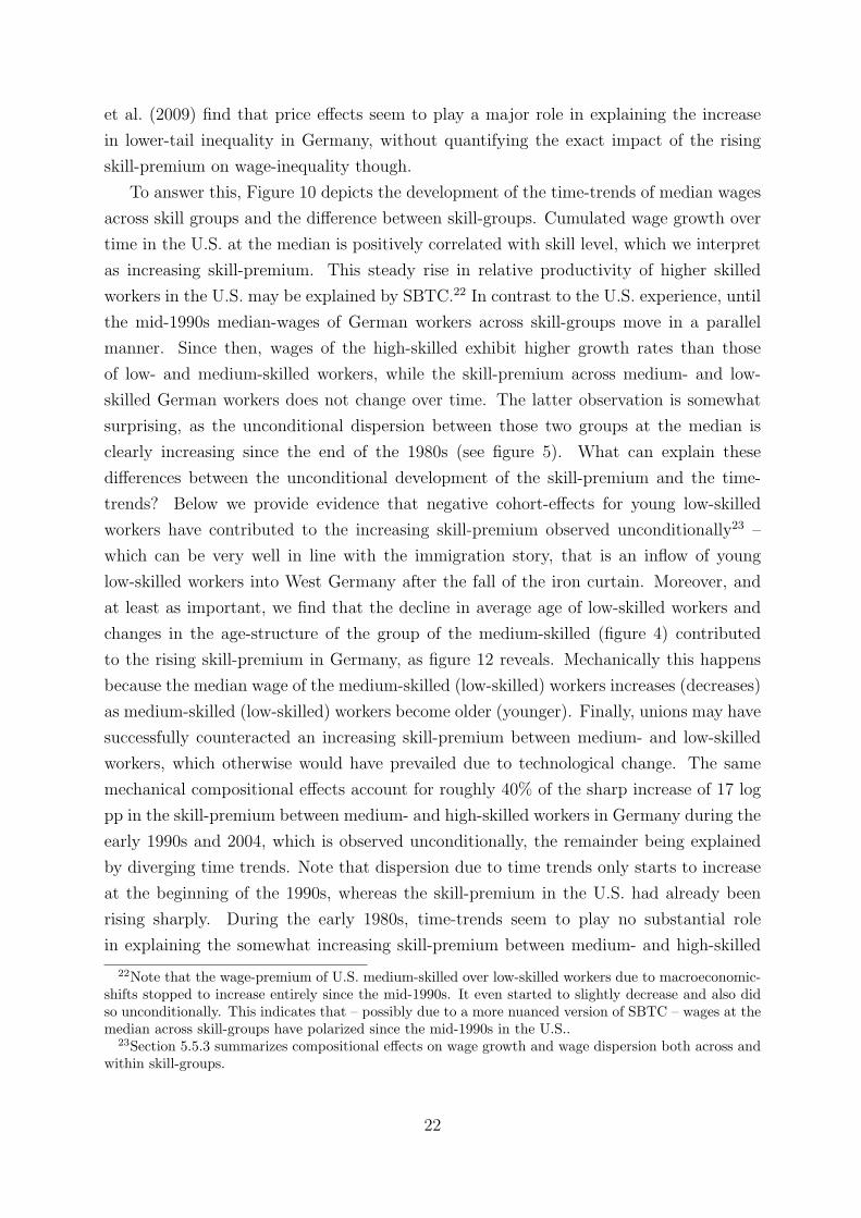
et al. (2009) find that price effects seem to play a major role in explaining the increase

in lower-tail inequality in Germany, without quantifying the exact impact of the rising

skill-premium on wage-inequality though.

To answer this, Figure 10 depicts the development of the time-trends of median wages

across skill groups and the difference between skill-groups. Cumulated wage growth over

time in the U.S. at the median is positively correlated with skill level, which we interpret

as increasing skill-premium. This steady rise in relative productivity of higher skilled

workers in the U.S. may be explained by SBTC.22 In contrast to the U.S. experience, until

the mid-1990s median-wages of German workers across skill-groups move in a parallel

manner. Since then, wages of the high-skilled exhibit higher growth rates than those

of low- and medium-skilled workers, while the skill-premium across medium- and low-

skilled German workers does not change over time. The latter observation is somewhat

surprising, as the unconditional dispersion between those two groups at the median is

clearly increasing since the end of the 1980s (see figure 5). What can explain these

differences between the unconditional development of the skill-premium and the time-

trends? Below we provide evidence that negative cohort-effects for young low-skilled

workers have contributed to the increasing skill-premium observed unconditionally23 –

which can be very well in line with the immigration story, that is an inflow of young

low-skilled workers into West Germany after the fall of the iron curtain. Moreover, and

at least as important, we find that the decline in average age of low-skilled workers and

changes in the age-structure of the group of the medium-skilled (figure 4) contributed

to the rising skill-premium in Germany, as figure 12 reveals. Mechanically this happens

because the median wage of the medium-skilled (low-skilled) workers increases (decreases)

as medium-skilled (low-skilled) workers become older (younger). Finally, unions may have

successfully counteracted an increasing skill-premium between medium- and low-skilled

workers, which otherwise would have prevailed due to technological change. The same

mechanical compositional effects account for roughly 40% of the sharp increase of 17 log

pp in the skill-premium between medium- and high-skilled workers in Germany during the

early 1990s and 2004, which is observed unconditionally, the remainder being explained

by diverging time trends. Note that dispersion due to time trends only starts to increase

at the beginning of the 1990s, whereas the skill-premium in the U.S. had already been

rising sharply. During the early 1980s, time-trends seem to play no substantial role

in explaining the somewhat increasing skill-premium between medium- and high-skilled

22Note that the wage-premium of U.S. medium-skilled over low-skilled workers due to macroeconomic-shifts stopped to increase entirely since the mid-1990s. It even started to slightly decrease and also didso unconditionally. This indicates that – possibly due to a more nuanced version of SBTC – wages at themedian across skill-groups have polarized since the mid-1990s in the U.S..

23Section 5.5.3 summarizes compositional effects on wage growth and wage dispersion both across andwithin skill-groups.

22

German workers observed unconditionally. While the change of the age-structure accounts

for some of the increase, so might changes in the cohort-structure.

For the U.S., we find that the time-trends describe the same patterns for the skill-

premia as the ones observed unconditionally – but not to the full extent. During the 1980s,

when the skill-premium between medium- and low-skilled U.S. workers increased, negative

cohort effects for the low-skilled were at work, perhaps again the effect of immigration.

The declining age of low-skilled workers also contributed to the rising wage-premium,

while the age-structure of medium-skilled workers was quite stable during the 1980s.

Regarding the wage-premium between high-skilled and medium-skilled in the U.S., we

see that the aging of the high-skilled contributed to an increasing premium during the

1980s. Overall, we thus observe somewhat similar patterns regarding the compositional

effects on the wage-premia for the U.S. and Germany.

Macroeconomic shifts are smooth functions of SBTC, institutional factors,24 and

supply-side factors, whereby the ways in which these functional arguments interact are a

priori not clear. Given that we observe two industrialized countries over the same period

of time, it is likely that they had access to the same technologies. Hence our results pro-

vide evidence that technological change alone is not able to explain rising wage inequality

as the wage-premium due to macro-economic shifts between German low- and medium-

skilled workers is constant over the entire period and comparing high- to medium-skilled

workers it only starts rising at the beginning of the 1990s. In fact, supply-side and insti-

tutional factors seem to play a key role in explaining the widening of the wage dispersion

between the skill-groups for Germany. A more promising approach to explain changes in

wage-inequality over time might thus be to consider, to a larger extent, the interaction

between labor market institutions, supply-side effects, and SBTC.25 Note that trends in

relative labor-supply across skill-groups as well as the age-pattern within skill groups are

showing very similar trends in both countries. This indicates that institutional factors –

and their interaction with SBTC – may be more important than supply-side factors in

explaining the cross-national differences.

5.5.2 Wage Dispersion within Skill-Groups

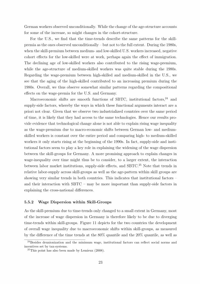
As the skill-premium due to time-trends only changed to a small extent in Germany, most

of the increase of wage dispersion in Germany is therefore likely to be due to diverging

time-trends within skill-groups. Figure 11 depicts for the two countries the development

of overall wage inequality due to macroeconomic shifts within skill-groups, as measured

by the difference of the time trends at the 80% quantile and the 20% quantile, as well as

24Besides deunionization and the minimum wage, institutional factors can reflect social norms andincentives set by tax-systems.

25This point has also been made by Lemieux (2008).

23

the wage dispersion in the upper and the lower part of the wage distribution, as measured

by the 80%-50% and 50%-20% difference, respectively.

Low-skilled workers in the U.S. experienced an astonishing decline in wage dispersion

in the lower part of the wage distribution starting in the mid-1980s. After a short period

of a rising 50%-20% difference of 2 log pp, wages at the median dropped more sharply then

wages at the 20% quantile until 1996 (and thereafter increased more slowly), resulting in

a decreasing dispersion of the lower part of the wage-distribution. Moreover, this decrease

is the driving force behind the decline of overall decreasing wage inequality, as measured

by the 80%-20% difference, as the inequality in the upper part was quite stable between

1980 and the end of the 1990s (thereafter wage inequality in the upper part decreased by

about 2 log pp). 26

Increasing wage inequality among U.S. medium-skilled workers since the early 1990s

masks a polarization pattern which starts as early as the end of the 1980s. Up until then,

wage inequality in the upper as well as the lower end of the wage distribution of this

group increased in a parallel way. Afterwards, the 80%-50% difference kept increasing

monotonically, while the 50%-20% difference started to fall. Mechanically, this results in

a small increase of the 80%-20% difference since the beginning of the 1990s.

Our results regarding wage inequality of U.S. low-skilled workers and the lower part

of U.S. medium-skilled workers for the 1980s may reflect ”episodic events”, such as the

declining real minimum wage and deunionization, and are thus in line with Card and

DiNardo (2002).27 The polarization of wages, beginning at the end of the 1980s, has also

been documented by Autor and Dorn (2009), who argue that the low-skill service sector is

the driving force. What is also interesting is the fact that the polarizing pattern – purely

due to macroeconomic shifts – sets in at least five years before the general recovery of

wages in the U.S. in the mid-1990s.

The highest increase of overall wage dispersion, as well as dispersion in the lower

part of the distribution, is observed for the group of high-skilled workers in the U.S. In

1986, the 80%-20% difference was at the same level as in 1979, then started to increase

monotonically until reaching a cumulated growth of 17 log pp in 2004, which is an increase

of about 1 log pp per year. Since 1986, we also observe a steep increase of the 80%-50%

difference after a drop by -2 log pp before. Accumulated wage dispersion over the entire

period is a slightly stronger for the 50%-20% difference (9 log pp), compared to 8 log pp

for the 80%-50% difference.28 Neither unions nor minimum wages are likely to have a large

26During the first half of the 1990s we find some support for within-skill-group polarization of wages, asthe 80%-50% difference slightly increases while the 50%-20% difference sharply drops during that period.

27A recent study by Chernozhukov et al. (2009), building upon DiNardo et al. (1996), shows thatminimum wage seems to play a larger role in 50-10 increase than deunioninzation. Autor et al. (2008),in the same line, concur that the decline of the minimum wage contributed to the rising lower tailwage-inequality.

28Note though that the 50%-20% difference plateaued during the second half of the 1990s, while the

24

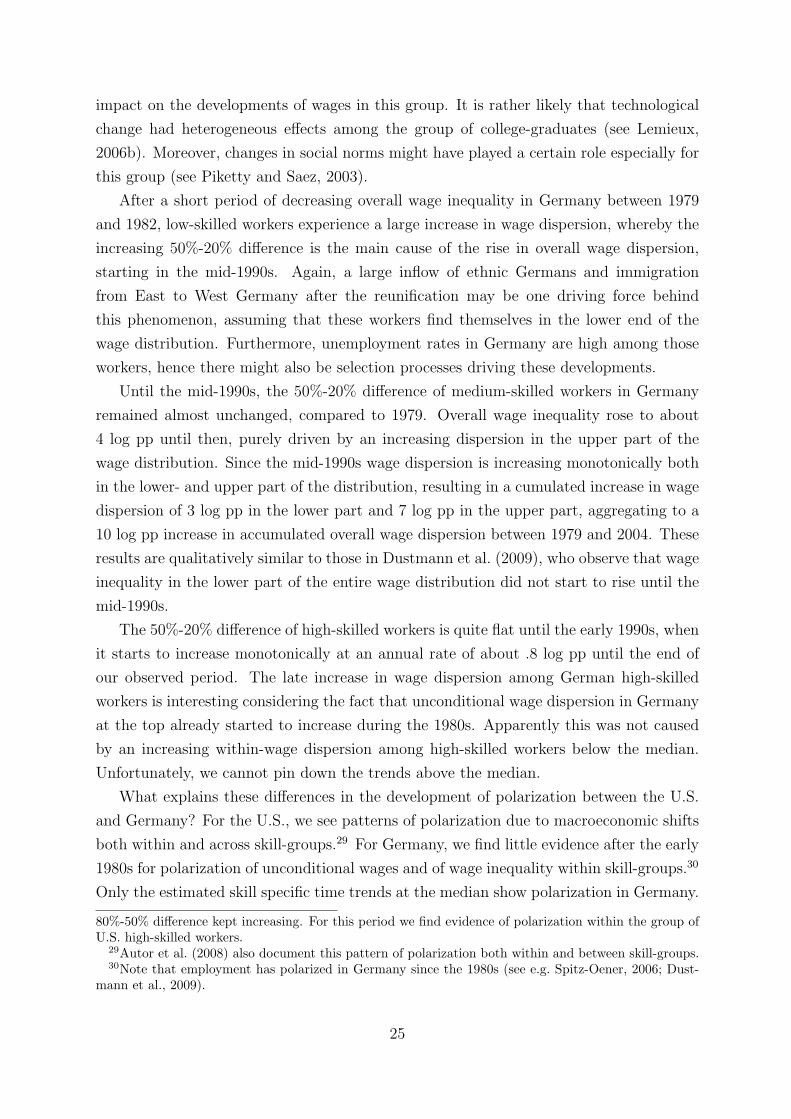
impact on the developments of wages in this group. It is rather likely that technological

change had heterogeneous effects among the group of college-graduates (see Lemieux,

2006b). Moreover, changes in social norms might have played a certain role especially for

this group (see Piketty and Saez, 2003).

After a short period of decreasing overall wage inequality in Germany between 1979

and 1982, low-skilled workers experience a large increase in wage dispersion, whereby the

increasing 50%-20% difference is the main cause of the rise in overall wage dispersion,

starting in the mid-1990s. Again, a large inflow of ethnic Germans and immigration

from East to West Germany after the reunification may be one driving force behind

this phenomenon, assuming that these workers find themselves in the lower end of the

wage distribution. Furthermore, unemployment rates in Germany are high among those

workers, hence there might also be selection processes driving these developments.

Until the mid-1990s, the 50%-20% difference of medium-skilled workers in Germany

remained almost unchanged, compared to 1979. Overall wage inequality rose to about

4 log pp until then, purely driven by an increasing dispersion in the upper part of the

wage distribution. Since the mid-1990s wage dispersion is increasing monotonically both

in the lower- and upper part of the distribution, resulting in a cumulated increase in wage

dispersion of 3 log pp in the lower part and 7 log pp in the upper part, aggregating to a

10 log pp increase in accumulated overall wage dispersion between 1979 and 2004. These

results are qualitatively similar to those in Dustmann et al. (2009), who observe that wage

inequality in the lower part of the entire wage distribution did not start to rise until the

mid-1990s.

The 50%-20% difference of high-skilled workers is quite flat until the early 1990s, when

it starts to increase monotonically at an annual rate of about .8 log pp until the end of

our observed period. The late increase in wage dispersion among German high-skilled

workers is interesting considering the fact that unconditional wage dispersion in Germany

at the top already started to increase during the 1980s. Apparently this was not caused

by an increasing within-wage dispersion among high-skilled workers below the median.

Unfortunately, we cannot pin down the trends above the median.

What explains these differences in the development of polarization between the U.S.

and Germany? For the U.S., we see patterns of polarization due to macroeconomic shifts

both within and across skill-groups.29 For Germany, we find little evidence after the early

1980s for polarization of unconditional wages and of wage inequality within skill-groups.30

Only the estimated skill specific time trends at the median show polarization in Germany.

80%-50% difference kept increasing. For this period we find evidence of polarization within the group ofU.S. high-skilled workers.

29Autor et al. (2008) also document this pattern of polarization both within and between skill-groups.30Note that employment has polarized in Germany since the 1980s (see e.g. Spitz-Oener, 2006; Dust-

mann et al., 2009).

25

As Fitzenberger (1999) and Dustmann et al. (2009) point out, the development of the

German wage structure is consistent with the SBTC story, if one allows for institutional

factors, such as unions and implicit minimum wages implied by the welfare state, which,

in comparison to the U.S., delayed the widening of the German wage dispersion in the

lower part for about ten years. A further explanation might be that social norms in

Germany have been different, an explanation which is put forward by Piketty and Saez

(2003) for other continental European countries as well. Along the line of the argument

brought forward by Chernozhukov et al. (2009) (i.e. the decline of the minimum wage

in the 1980s in the U.S. counteracted the polarization of wages during that period), it

is conceivable that the deunionization in Germany during the 1990s and the early 2000s

counteracted a polarization of wages.

5.5.3 Compositional Effects on Wage growth and Inequality

Figure 6 depicts the life-cycle profiles of wage growth conditional on education, showing

that inequality varies by age. To illustrate this, figure 12 plots the effect of the changing

age structure on wage growth and (implicitly) on wage dispersion. This is done by using

the estimates of the life-cycle profile of wages and the changing distribution of ages to

calculate the implied change in wages. The increase of the mean ages both of medium-

and high-skilled workers in the U.S. reflect the changes of the age structure which result in

increasing wages in these two subgroups. However, wage inequality only slightly increases

due to the changing age structure. The trend for low-skilled workers in the U.S. is re-

versed: The mean age decreases between 1979 and 2004, and changes in the age-structure

lead to decreasing wages as well as less wage-inequality over time, being mainly driven by

declining wage dispersion in the lower part of the wage distribution. Comparing the devel-

opment of the wages at the medians across skill-groups, it is clear that, first, throughout

the entire period the changing age structure among low- and medium-skilled U.S. work-

ers led to an increasing skill-premium between medium and low, second, that during the

1980s, the aging of high-skilled workers led to an increasing skill-premium between high

and medium.

For Germany the results differ for the low-skilled. Although the age-pattern is quali-

tatively the same between 1979 and 2004 compared to the U.S., the rejuvenation of this

skill-group, indicated by a decrease of the mean age, leads to an increasing within wage

dispersion over time, as the 20% quantile in this group experiences the largest life-cycle

wage growth. The changing age-structure of medium- and high-skilled workers in Ger-

many, indicated by the rise of the mean age starting in the late 1990s, mechanically leads

to an increasing wages for both groups. The age-decomposition effect only plays a minor

role in explaining changes of wage dispersion conditional on education though. The aging

26

of German medium-skilled workers since the early 1990s led to an increasing skill-premium

between low- and medium-skilled workers, which, as we have shown above, is not due to

macro-economic shifts. Similarly, differences in the pattern of aging between medium-

and high-skilled workers led to an increasing skill-premium between those two groups.

Figures 13 and 14 depict the impact of the inflow and outflow of the cohorts on skill-

specific wage growth and dispersion, respectively. The latter graphs show that starting

in the early 1990s, the change in the cohort structure supports the catching-up process of

both wages at the median and the 20% quantile to wages at the 80% quantile in the group

of low-skilled workers in the U.S.. The 80-50 and 80-20 difference of wages had increased

before, though, due to cohort-effects. Contrary to that, cohort-effects in Germany for the

group of low-skilled led to an increasing wage dispersion of about 5 log pp throughout

the entire wage-distribution between 1992 and 2004, while before the early 1990s, cohort

effects led to a decreasing wage dispersion, with the movements of the 80-20 difference

mainly being driven by changes of the wage dispersion in the lower part. Cohort effects for

medium- and high-skilled workers affect wage dispersion somewhat less in both countries.

Relatively to the oldest and the youngest cohorts, those in the middle seem to exhibit

higher cohort-specific wage dispersion, driven mostly by positive cohort-effects at the

median and the 80% quantile. In the middle of the observed period, the presence of these

cohorts in the middle is strongest, resulting in the strongest increase in wage dispersion

within skill groups. Based on figure 13, the sharp drop of cohort effects among low-skilled

German workers mechanically increases the wage-premium between low- and medium-

skilled workers in Germany. Compositional effects regarding the cohort structure also

seem to increase the skill-premium between high-and medium-skilled workers in Germany

since the early 1990s. For the U.S., these kind of compositional effects seem to play only

a minor role.

5.6 Employment Growth

In order to describe employment growth along the wage distribution and to detect possible

polarization of employment, we use a method similar to that proposed by Card et al.

(1999). We rank the age-education cells across skill-groups for a base year according to

the cells unconditional median wages, normalized by the estimated age-specific life-cycle

wage growth of the specific cells.31 Then we calculate the cumulated relative employment

growth of each cell over the next ten years.32 Our age variable is discrete, ranging between

31Cells whose median wages are top-coded – this happens frequently for the group of high-skilledGerman workers – are given the highest ranks, whereby the general pattern of the graphs is not affectedby the chosen order. We thus draw random numbers to determine the order of the ranks at the top-end.

32Note that in the latter period different workers are in those cells, as the age is held constant for eachcell.

27

25 and 55, and we distinguish between three educational levels, which yields 93 cells for

this analysis, which Card et al. (1999) interpret as ”skill-groups”. The base years we

choose are 1979, 1984, 1989, and 1999. The results are depicted in figures 15 and 16.

For the base years 1979 and 1984, relative changes in employment in both economies

is a monotonically increasing function of the rank of wages in the base year. We find

evidence of employment polarization in Germany starting with the base year 1989, which

becomes more pronounced for the base year 1994. This means that for the latter two

base years, age-education cells which are ranked at the bottom exhibit higher growth

rates than those at the middle, while the highest ranked age-education exhibit the largest

growth rates. For the U.S. we observe a similar pattern of polarization starting in the

second half of the 1990s. There are striking similarities in the four graphs between the

U.S. and Germany.

This simple analysis helps us to separate demand-side vs. supply-side stories. In the

U.S., we observe polarization in wages and employment, as a nuanced version of the

SBTC-story would suggest, while in Germany we observe polarization in employment but

little evidence for polarization in wages. The latter observation might also be caused by

immigration into West Germany for example. Hence, only for the U.S. the broad findings

are consistent with a pure demand-side story.

6 Conclusion

This paper examines trends in wage inequality in the U.S. and Germany. A cross-national

comparison of these trends is important as some explanations for the widening gap in

wages between highly skilled workers and lower skilled workers, for example SBTC, should

apply to both economies. The methods we employ enable us to separately identify life-

cycle wage profiles, trends in wages (due to macroeconomic shifts), and cohort wage

effects.

We find that, for workers of all skill levels in the U.S. and for higher skilled workers

in Germany, there is increasing wage inequality over the life cycle. In contrast, for low-

skilled workers in Germany there is decreasing wage inequality over the life cycle. The

changing age structure of the workforce has important implications for trends in wage

inequality in both the U.S. and in Germany. Aging among higher skilled workers tends to

increase both wage levels and wage inequality in both countries. However, the decline in

age among low-skilled workers has different effects in the U.S. compared to Germany. In

the U.S., this decline in age has the effect of lowering wages and lowering wage inequality.

However, in Germany a decline in age tends to lower wages but increases wage inequality.

There exist important cohort effects for Germany. Both the old and the young cohorts

of workers have sizeable negative cohort effects. These effects could be the result of supply-

28

side factors such as immigration, cohort size, or selection into skill-group. In the U.S., by

contrast, the size of the cohort effects is substantially smaller.

The time trends in wages tend to favor highly skilled workers in both the U.S. and

in Germany. In the U.S. there were secular declines in wages until the mid-1990s for

low- and medium-skilled workers when these trends reversed. In Germany, we see the

opposite pattern – rising secular trends in wages until the mid-1990s and a flattening (at

the median) or a decline (at the 20% quantile) in wages afterwards. The result of these

trends is that in recent years we have seen an increase in wage inequality among low-

skilled workers in Germany and a decline in wage inequality among lower skilled workers

in the U.S..

We also find a rising skill premium in both the U.S. and in Germany. In Germany,

however, the rising skill premium between medium- and low-skilled workers is entirely the

result of cohort effects and aging effects. The rise for high-skilled compared to medium-

skilled workers is mostly restricted to the period after the mid-1990s.

In the U.S., we see faster wage growth at the top (80% quantile) and bottom (20%

quantile). This has been interpreted as evidence of polarization in previous studies (e.g.

Autor et al., 2008). We see only little evidence of wage polarization in Germany after

the early 1980s, with the exception being that conditional time trends at the median are

quite similar for medium-skilled and low-skilled workers.

Summing up, there is a lot of similar evidence in wages – and in particular in em-

ployment – in the U.S. and Germany which is consistent with a technology driven polar-

ization of labor market. However, the patterns in wage inequality in the two countries

differ strongly, so that it is unlikely that technology effects alone – which presumably are

common across countries – can explain the empirical findings. Episodic changes resulting

from changes in institutional factors such as unionization or the minimum wage may ex-

plain the differences, which are partly reflected in the cross-country differences in cohort

effects. Institutional factors in Germany might have led to increased inequality among

less skilled groups after 1985, which more than offset technology driven trends in the lower

part of the wage distribution. Another possibility is that SBTC interacts in important

ways with institutional factors and that differences in institutions across economies are

the reason why we observe different trends in inequality across the U.S. and Germany.

29

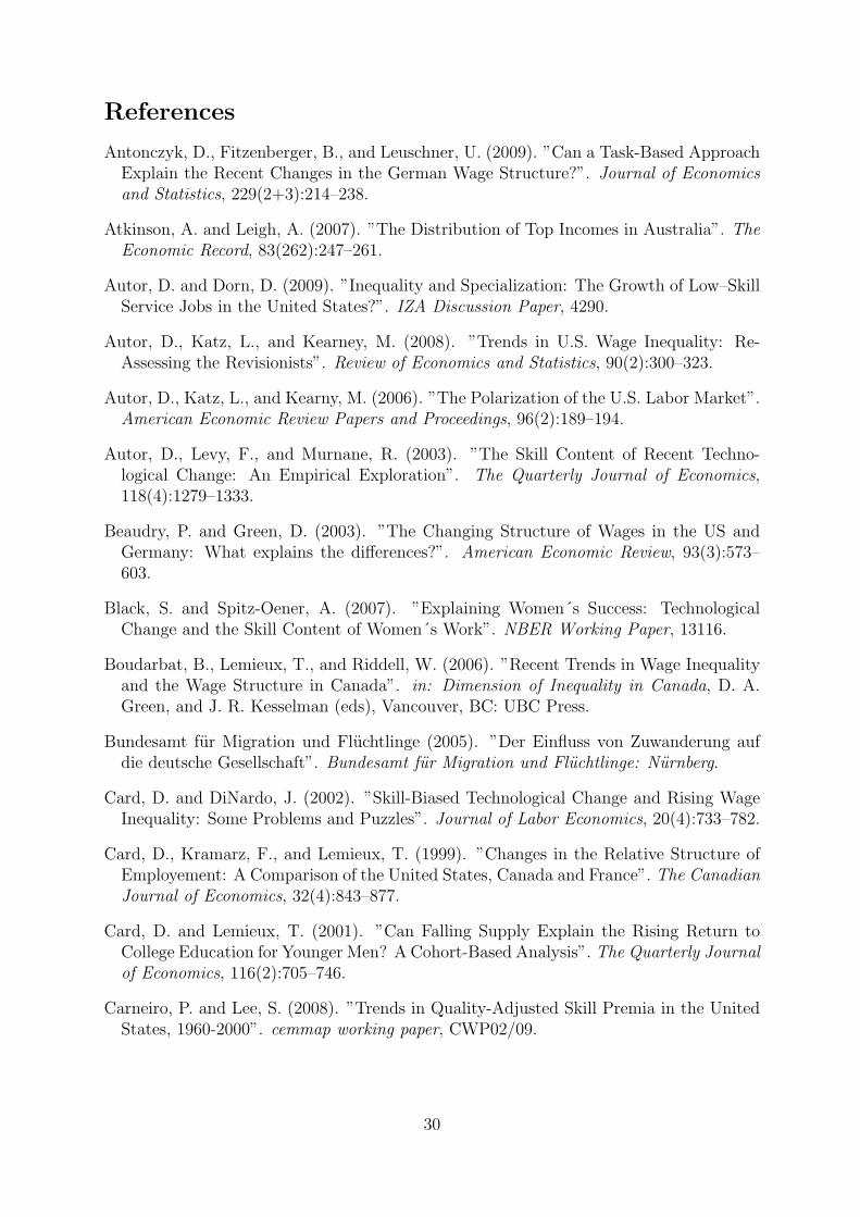
References

Antonczyk, D., Fitzenberger, B., and Leuschner, U. (2009). ”Can a Task-Based ApproachExplain the Recent Changes in the German Wage Structure?”. Journal of Economicsand Statistics, 229(2+3):214–238.

Atkinson, A. and Leigh, A. (2007). ”The Distribution of Top Incomes in Australia”. TheEconomic Record, 83(262):247–261.

Autor, D. and Dorn, D. (2009). ”Inequality and Specialization: The Growth of Low–SkillService Jobs in the United States?”. IZA Discussion Paper, 4290.

Autor, D., Katz, L., and Kearney, M. (2008). ”Trends in U.S. Wage Inequality: Re-Assessing the Revisionists”. Review of Economics and Statistics, 90(2):300–323.

Autor, D., Katz, L., and Kearny, M. (2006). ”The Polarization of the U.S. Labor Market”.American Economic Review Papers and Proceedings, 96(2):189–194.

Autor, D., Levy, F., and Murnane, R. (2003). ”The Skill Content of Recent Techno-logical Change: An Empirical Exploration”. The Quarterly Journal of Economics,118(4):1279–1333.

Beaudry, P. and Green, D. (2003). ”The Changing Structure of Wages in the US andGermany: What explains the differences?”. American Economic Review, 93(3):573–603.

Black, S. and Spitz-Oener, A. (2007). ”Explaining Women´s Success: TechnologicalChange and the Skill Content of Women´s Work”. NBER Working Paper, 13116.

Boudarbat, B., Lemieux, T., and Riddell, W. (2006). ”Recent Trends in Wage Inequalityand the Wage Structure in Canada”. in: Dimension of Inequality in Canada, D. A.Green, and J. R. Kesselman (eds), Vancouver, BC: UBC Press.

Bundesamt fur Migration und Fluchtlinge (2005). ”Der Einfluss von Zuwanderung aufdie deutsche Gesellschaft”. Bundesamt fur Migration und Fluchtlinge: Nurnberg.

Card, D. and DiNardo, J. (2002). ”Skill-Biased Technological Change and Rising WageInequality: Some Problems and Puzzles”. Journal of Labor Economics, 20(4):733–782.

Card, D., Kramarz, F., and Lemieux, T. (1999). ”Changes in the Relative Structure ofEmployement: A Comparison of the United States, Canada and France”. The CanadianJournal of Economics, 32(4):843–877.

Card, D. and Lemieux, T. (2001). ”Can Falling Supply Explain the Rising Return toCollege Education for Younger Men? A Cohort-Based Analysis”. The Quarterly Journalof Economics, 116(2):705–746.

Carneiro, P. and Lee, S. (2008). ”Trends in Quality-Adjusted Skill Premia in the UnitedStates, 1960-2000”. cemmap working paper, CWP02/09.

30

Chamberlain, G. (1994). ”Quantile Regression, Censoring and the Structure of Wages”.In Sims, C., editor, Advances in Econometrics: Sixth World Congress. EconometricSociety Monograph, Volume 1.

Chernozhukov, V., Fernandez, I., and Melly, B. (2009). ”Inference on CounterfactualDistributions”. MIT Working Paper, 08-16.

DiNardo, J., Fortin, N., and Lemieux, T. (1996). ”Labor Markets Institutions and the Dis-tribution of Wages, 1973-1992: A Semiparametric Approach”. Econometrica, 64:1001–1044.

Dustmann, C., Ludsteck, J., and Schonberg, U. (2009). ”Revisiting the German WageStructure”. The Quarterly Journal of Economics, Vol. 124(2):843–881.

Fitzenberger, B. (1999). ”Wages and Employment Across Skill Groups: An Analysis forWest Germany”. Physica/Springer, Heidelberg.

Fitzenberger, B., Hujer, R., MaCurdy, T., and Schnabel, R. (2001). ”Testing for UniformWage Trends in West Germany: A Cohort Analysis Using Quantile Regressions forCensored Data”. Empirical Economics, 26(1):41–86.

Fitzenberger, B., Kohn, K., and Wang, Q. (2010). ”The Erosion of Union Membershipin Germany: Determinants, Densities, Decompositions”. Journal of Population Eco-nomics, forthcoming.

Fitzenberger, B. and Wunderlich, G. (2002). ”Gender Wage Differences in West Germany:A Cohort Analysis”. German Economic Review, 3(4):379–414.

Fuchs-Schundeln, N. and Schundeln, M. (2009). ”Who stays, who goes, who returns?East-West migration within Germany since reunification”. Economics of Transition,17(4):703–738.

Gernandt, J. and Pfeiffer, F. (2007). ”Rising Wage Inequality in Germany”. Journal ofEconomics and Statistics, 227(4):358–380.

Goos, M. and Manning, A. (2007). ”Lousy and Lovely Jobs: The Rising Polarization ofWork in Britain”. Review of Economics and Statistics, 89:118–133.

Gosling, A., Machin, S., and Meghir, C. (2000). ”The Changing Distribution of MaleWages in the U.K.”. Review of Economic Studies, 67:635–666.

Katz, L. and Autor, D. (1999). ”Changes in the Wage Structure and Earnings Inequal-ity”. Ashenfelter, O. and D. Card (eds), Handbook of Labor Economics., 3A:1463–1555,North Holland, Amsterdam.

Koenker, R. and Bassett, G. (1978). ”Regression Quantiles”. Econometrica, 46(1):33–50.

Kohn, K. (2006). ”Rising Wage Dispersion, After All! The German Wage Structure atthe Turn of the Century”. ZEW Discussion Paper, (06-031).

Lemieux, T. (2006a). ”Increased Residual Wage Inequality: Composition Effects, NoisyData, or Rising Demand for Skill”. American Economic Review, 96:461–498.

31

Lemieux, T. (2006b). ”Postsecondary Education and Increasing Wage Inequality”. Amer-ican Economic Review Papers and Proceedings, 96(2):195–199.

Lemieux, T. (2008). ”The Changing Nature of Wage Inequality”. Journal of PopulationEconomics, 21:21–48.

Machin, S. and Van Reenen, J. (2008). ”Changes in Wage Inequality”. Durlauf, S.N andL.E. Blume (eds), The New Palgrave Dictionary of Economics., Second Edition.

MaCurdy, T. and Mroz, T. (1995). ”Measuring Macroeconomic Shifts in Wages fromCohort Specifications”. Unpublished Manuscript, Stanford University and University ofNorth Carolina.

Manning, A. (2004). ”We Can Work It Out: the Impact of Technological Change on theDemand for Low-Skill Workers”. Scottish Journal of Political Economy, 51(5):581–608.

OECD (2006). ”Education at a glance 2006”. OECD, Paris.

Piketty, T. and Saez, E. (2003). ”Income Inequality in the United States, 1913-1998”.The Quarterly Journal of Economics, Vol. 118(1):1–39.

Prasad, U. (2004). The Unbearable Stability of the German Wage Structure: Evidenceand Interpretation. IMF Staff Paper, 51(2):354–385.

Spitz-Oener, A. (2006). ”Technical Change, Job Tasks, and Rising Educational Demands:Looking Outside the Wage Structure”. Journal of Labor Economics, 24(2):235–270.

32

Appendix

Males U.S.

1980 1985 1990 1995 2000 2005

−0.

2−

0.1

0.0

0.1

0.2

YEAR

Cum

. Wag

e G

row

th

205080

Males Germany

1980 1985 1990 1995 2000 2005

0.0

0.1

0.2

0.3

YEARC

um. W

age

Gro

wth

205080

Males U.S.

1980 1985 1990 1995 2000 2005

−0.

050.

000.

050.

100.

150.

200.

25

YEAR

Cum

. Gro

wth

of D

iffer

ence

s

80−2080−5050−20

Males Germany

1980 1985 1990 1995 2000 2005

−0.

050.

000.

050.

100.

150.

200.

25

YEAR

Cum

. Gro

wth

of D

iffer

ence

s

80−2080−5050−20

Figure 1: Total Unconditional Cumulated Wage growth at 20%, 50%, 80% quantiles andquantile differences, 1979-2004 for males, left: U.S., right: Germany

33

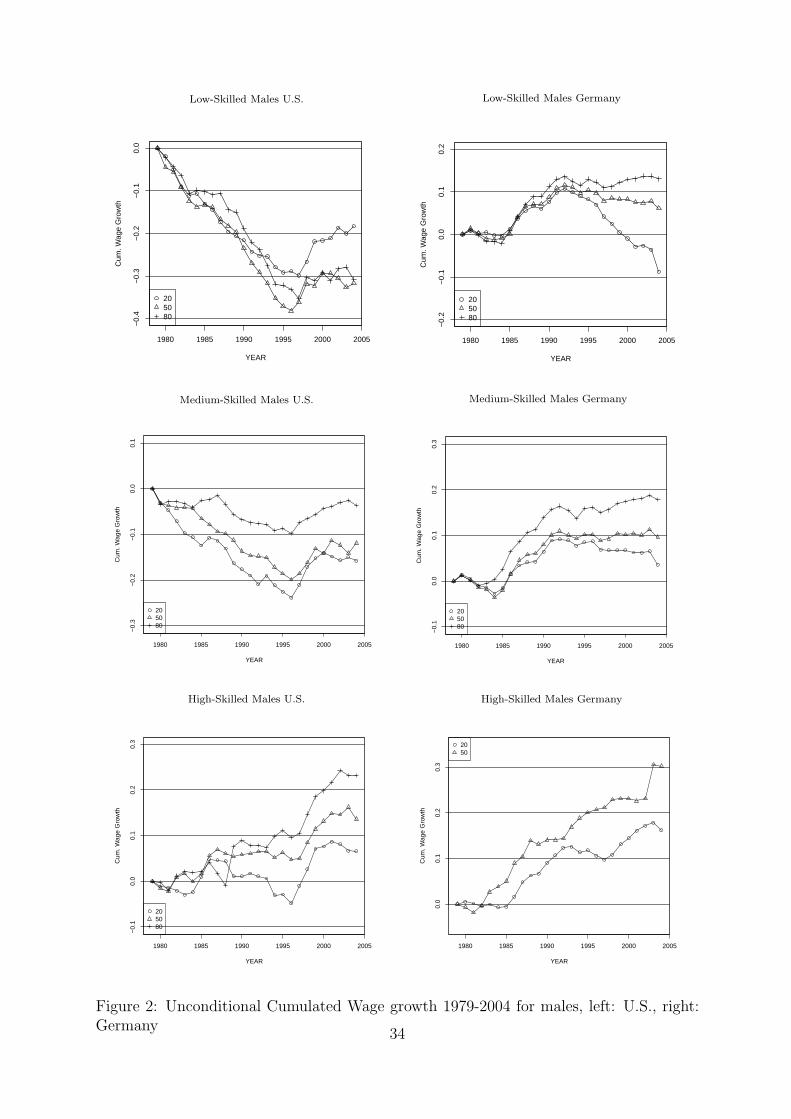
Low-Skilled Males U.S.

1980 1985 1990 1995 2000 2005

−0.

4−

0.3

−0.

2−

0.1

0.0

YEAR

Cum

. Wag

e G

row

th

205080

Low-Skilled Males Germany

1980 1985 1990 1995 2000 2005

−0.

2−

0.1

0.0

0.1

0.2

YEAR

Cum

. Wag

e G

row

th

205080

Medium-Skilled Males U.S.

1980 1985 1990 1995 2000 2005

−0.

3−

0.2

−0.

10.

00.

1

YEAR

Cum

. Wag

e G

row

th

205080

Medium-Skilled Males Germany

1980 1985 1990 1995 2000 2005

−0.

10.

00.

10.

20.

3

YEAR

Cum

. Wag

e G

row

th

205080

High-Skilled Males U.S.

1980 1985 1990 1995 2000 2005

−0.

10.

00.

10.

20.

3

YEAR

Cum

. Wag

e G

row

th

205080

High-Skilled Males Germany

1980 1985 1990 1995 2000 2005

0.0

0.1

0.2

0.3

YEAR

Cum

. Wag

e G

row

th

2050

Figure 2: Unconditional Cumulated Wage growth 1979-2004 for males, left: U.S., right:Germany

34

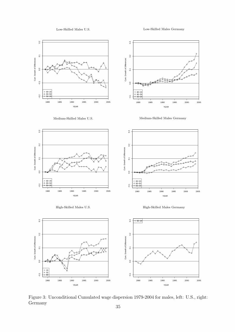
Low-Skilled Males U.S.

1980 1985 1990 1995 2000 2005

−0.

2−

0.1

0.0

0.1

0.2

YEAR

Cum

. Gro

wth

of D

iffer

ence

s

80−2080−5050−20

Low-Skilled Males Germany

1980 1985 1990 1995 2000 2005

−0.

10.

00.

10.

20.

3

YEAR

Cum

. Gro

wth

of D

iffer

ence

s

80−2080−5050−20

Medium-Skilled Males U.S.

1980 1985 1990 1995 2000 2005

−0.

10.

00.

10.

20.

3

YEAR

Cum

. Gro

wth

of D

iffer

ence

s

80−2080−5050−20

Medium-Skilled Males Germany

1980 1985 1990 1995 2000 2005

−0.

10.

00.

10.

20.

3

YEAR

Cum

. Gro

wth

of D

iffer

ence

s

80−2080−5050−20

High-Skilled Males U.S.

1980 1985 1990 1995 2000 2005

−0.

10.

00.

10.

20.

3

YEAR

Cum

. Gro

wth

of D

iffer

ence

s

205080

High-Skilled Males Germany

1980 1985 1990 1995 2000 2005

−0.

10.

00.

10.

20.

3

YEAR

Cum

. Gro

wth

of D

iffer

ence

s

50−20

Figure 3: Unconditional Cumulated wage dispersion 1979-2004 for males, left: U.S., right:Germany

35

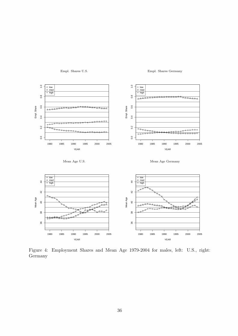
Empl. Shares U.S.

1980 1985 1990 1995 2000 2005

0.0

0.2

0.4

0.6

0.8

1.0

YEAR

Em

pl. S

hare

lowmedhigh

Empl. Shares Germany

1980 1985 1990 1995 2000 2005

0.0

0.2

0.4

0.6

0.8

1.0

YEAR

Em

pl. S

hare

lowmedhigh

Mean Age U.S.

1980 1985 1990 1995 2000 2005

3638

4042

44

YEAR

Mea

n A

ge

lowmedhigh

Mean Age Germany

1980 1985 1990 1995 2000 2005

3638

4042

44

YEAR

Mea

n A

ge

lowmedhigh

Figure 4: Employment Shares and Mean Age 1979-2004 for males, left: U.S., right:Germany

36

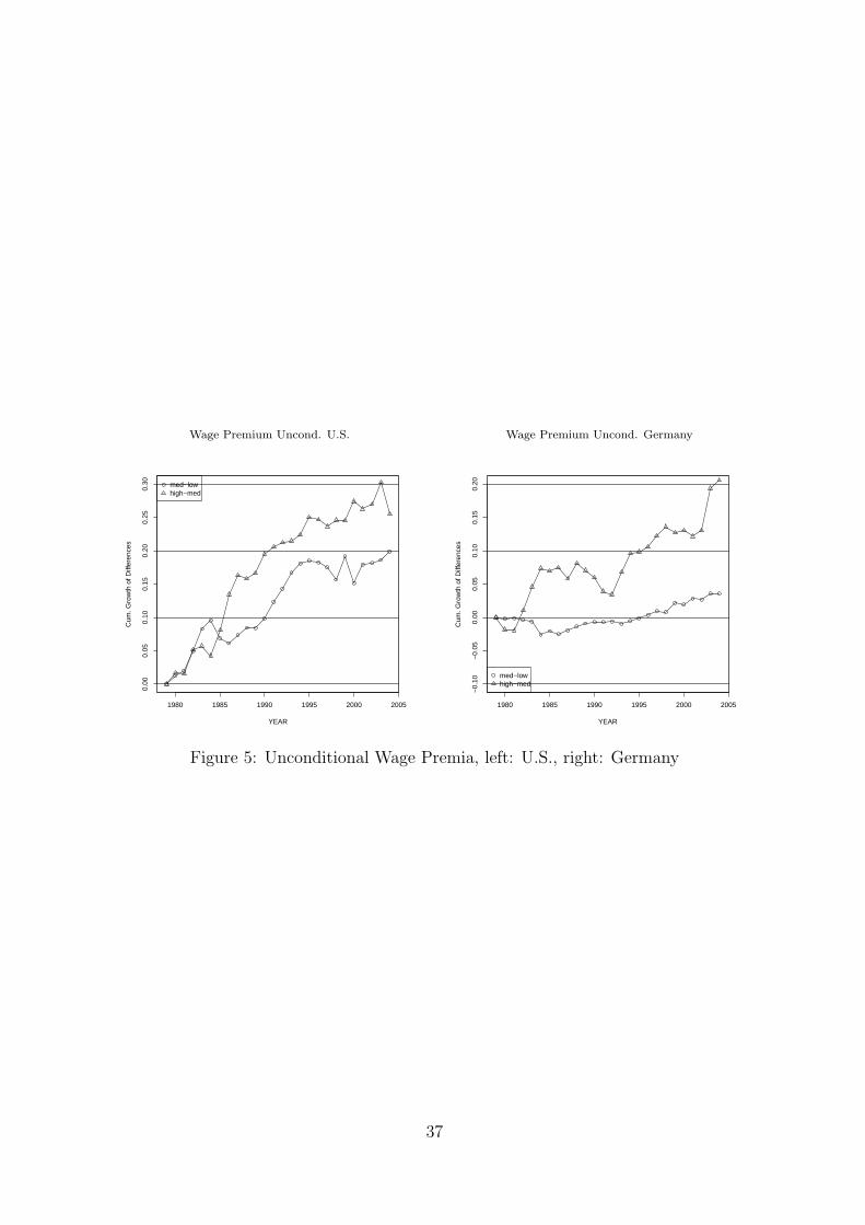
Wage Premium Uncond. U.S.

1980 1985 1990 1995 2000 2005

0.00

0.05

0.10

0.15

0.20

0.25

0.30

YEAR

Cum

. Gro

wth

of D

iffer

ence

s

med−lowhigh−med

Wage Premium Uncond. Germany

1980 1985 1990 1995 2000 2005

−0.

10−

0.05

0.00

0.05

0.10

0.15

0.20

YEAR

Cum

. Gro

wth

of D

iffer

ence

s

med−lowhigh−med

Figure 5: Unconditional Wage Premia, left: U.S., right: Germany

37

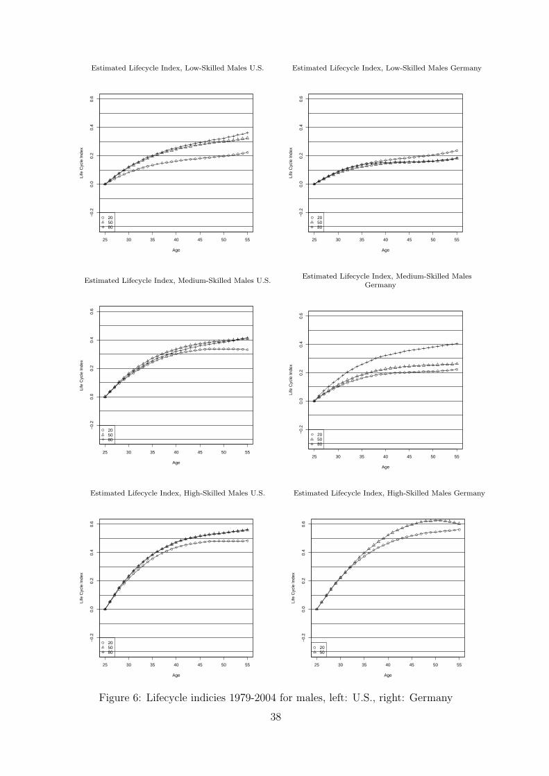
Estimated Lifecycle Index, Low-Skilled Males U.S.

25 30 35 40 45 50 55

−0.

20.

00.

20.

40.

6

Age

Life

Cyc

le In

dex

205080

Estimated Lifecycle Index, Low-Skilled Males Germany

25 30 35 40 45 50 55

−0.

20.

00.

20.

40.

6

Age

Life

Cyc

le In

dex

205080

Estimated Lifecycle Index, Medium-Skilled Males U.S.

25 30 35 40 45 50 55

−0.

20.

00.

20.

40.

6

Age

Life

Cyc

le In

dex

205080

Estimated Lifecycle Index, Medium-Skilled MalesGermany

25 30 35 40 45 50 55

−0.

20.

00.

20.

40.

6

Age

Life

Cyc

le In

dex

205080

Estimated Lifecycle Index, High-Skilled Males U.S.

25 30 35 40 45 50 55

−0.

20.

00.

20.

40.

6

Age

Life

Cyc

le In

dex

205080

Estimated Lifecycle Index, High-Skilled Males Germany

25 30 35 40 45 50 55

−0.

20.

00.

20.

40.

6

Age

Life

Cyc

le In

dex

2050

Figure 6: Lifecycle indicies 1979-2004 for males, left: U.S., right: Germany

38

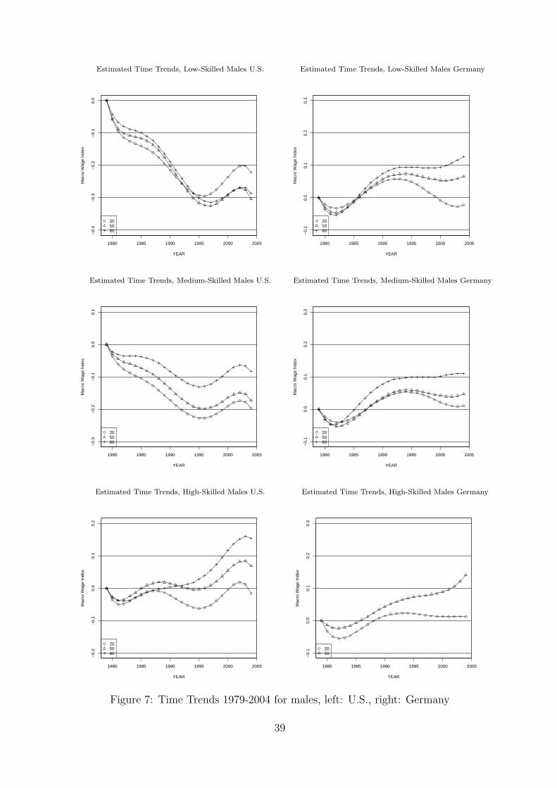
Estimated Time Trends, Low-Skilled Males U.S.

1980 1985 1990 1995 2000 2005

−0.

4−

0.3

−0.

2−

0.1

0.0

YEAR

Mac

ro W

age

Inde

x

205080

Estimated Time Trends, Low-Skilled Males Germany

1980 1985 1990 1995 2000 2005

−0.

10.

00.

10.

20.

3

YEAR

Mac

ro W

age

Inde

x

205080

Estimated Time Trends, Medium-Skilled Males U.S.

1980 1985 1990 1995 2000 2005

−0.

3−

0.2

−0.

10.

00.

1

YEAR

Mac

ro W

age

Inde

x

205080

Estimated Time Trends, Medium-Skilled Males Germany

1980 1985 1990 1995 2000 2005

−0.

10.

00.

10.

20.

3

YEAR

Mac

ro W

age

Inde

x

205080

Estimated Time Trends, High-Skilled Males U.S.

1980 1985 1990 1995 2000 2005

−0.

2−

0.1

0.0

0.1

0.2

YEAR

Mac

ro W

age

Inde

x

205080

Estimated Time Trends, High-Skilled Males Germany

1980 1985 1990 1995 2000 2005

−0.

10.

00.

10.

20.

3

YEAR

Mac

ro W

age

Inde

x

2050

Figure 7: Time Trends 1979-2004 for males, left: U.S., right: Germany

39

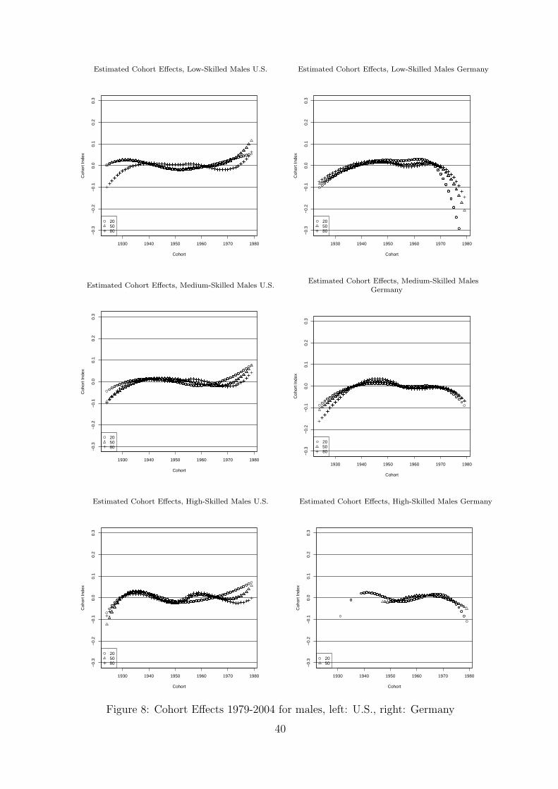
Estimated Cohort Effects, Low-Skilled Males U.S.

1930 1940 1950 1960 1970 1980

−0.

3−

0.2

−0.

10.

00.

10.

20.

3

Cohort

Coh

ort I

ndex

205080

Estimated Cohort Effects, Low-Skilled Males Germany

1930 1940 1950 1960 1970 1980

−0.

3−

0.2

−0.

10.

00.

10.

20.

3

Cohort

Coh

ort I

ndex

205080

Estimated Cohort Effects, Medium-Skilled Males U.S.

1930 1940 1950 1960 1970 1980

−0.

3−

0.2

−0.

10.

00.

10.

20.

3

Cohort

Coh

ort I

ndex

205080

Estimated Cohort Effects, Medium-Skilled MalesGermany

1930 1940 1950 1960 1970 1980

−0.

3−

0.2

−0.

10.

00.

10.

20.

3

Cohort

Coh

ort I

ndex

205080

Estimated Cohort Effects, High-Skilled Males U.S.

1930 1940 1950 1960 1970 1980

−0.

3−

0.2

−0.

10.

00.

10.

20.

3

Cohort

Coh

ort I

ndex

205080

Estimated Cohort Effects, High-Skilled Males Germany

1930 1940 1950 1960 1970 1980

−0.

3−

0.2

−0.

10.

00.

10.

20.

3

Cohort

Coh

ort I

ndex

2050

Figure 8: Cohort Effects 1979-2004 for males, left: U.S., right: Germany

40

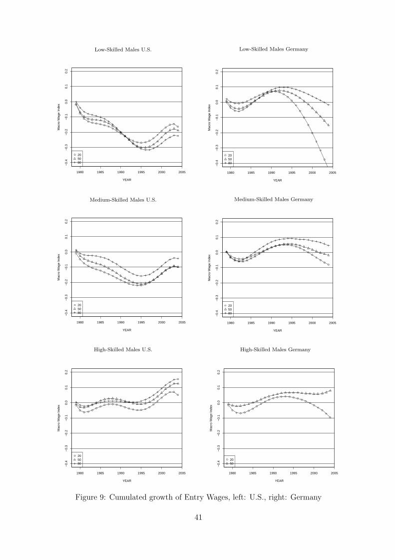
Low-Skilled Males U.S.

1980 1985 1990 1995 2000 2005

−0.

4−

0.3

−0.

2−

0.1

0.0

0.1

0.2

YEAR

Mac

ro W

age

Inde

x

205080

Low-Skilled Males Germany

1980 1985 1990 1995 2000 2005

−0.

4−

0.3

−0.

2−

0.1

0.0

0.1

0.2

YEAR

Mac

ro W

age

Inde

x

205080

Medium-Skilled Males U.S.

1980 1985 1990 1995 2000 2005

−0.

4−

0.3

−0.

2−

0.1

0.0

0.1

0.2

YEAR

Mac

ro W

age

Inde

x

205080

Medium-Skilled Males Germany

1980 1985 1990 1995 2000 2005

−0.

4−

0.3

−0.

2−

0.1

0.0

0.1

0.2

YEAR

Mac

ro W

age

Inde

x

205080

High-Skilled Males U.S.

1980 1985 1990 1995 2000 2005

−0.

4−

0.3

−0.

2−

0.1

0.0

0.1

0.2

YEAR

Mac

ro W

age

Inde

x

205080

High-Skilled Males Germany

1980 1985 1990 1995 2000 2005

−0.

4−

0.3

−0.

2−

0.1

0.0

0.1

0.2

YEAR

Mac

ro W

age

Inde

x

2050

Figure 9: Cumulated growth of Entry Wages, left: U.S., right: Germany

41

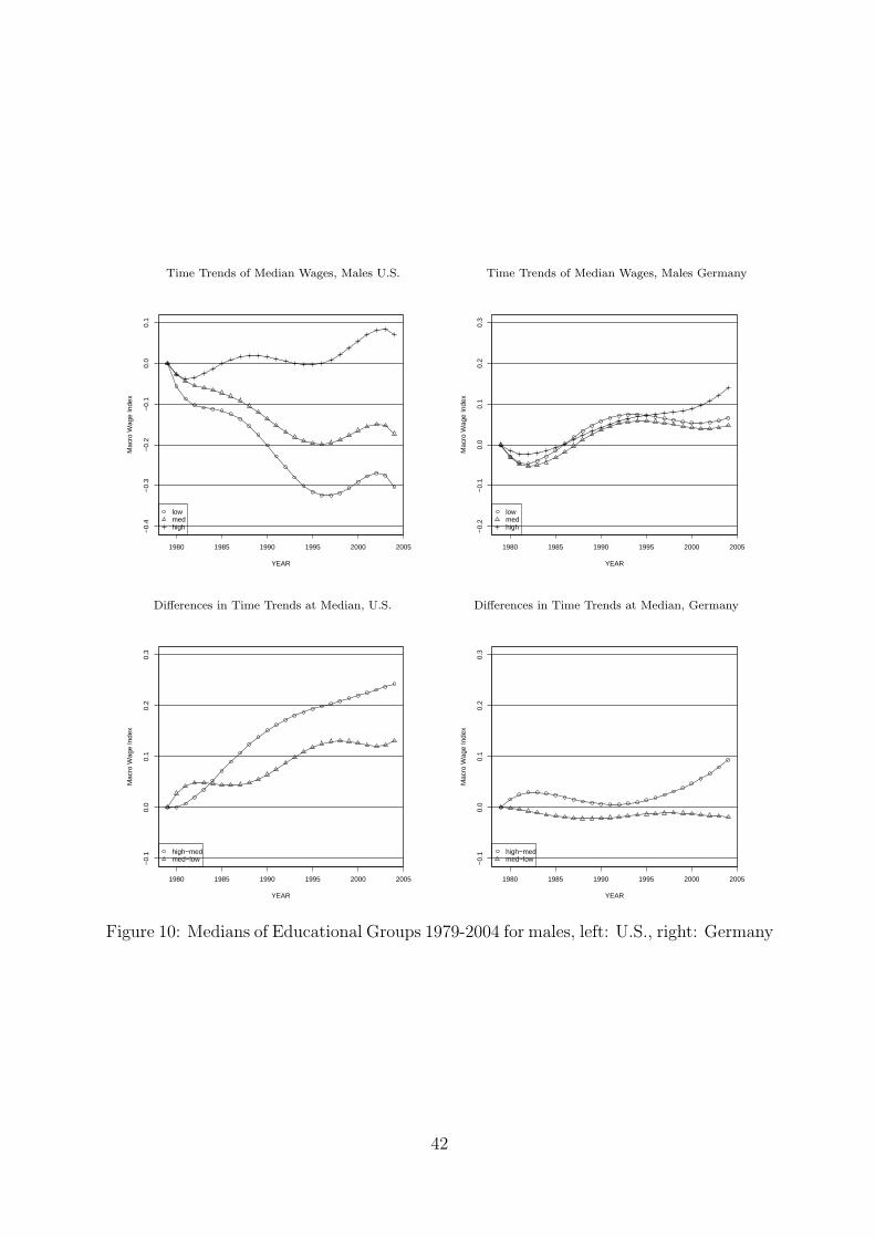
Time Trends of Median Wages, Males U.S.

1980 1985 1990 1995 2000 2005

−0.

4−

0.3

−0.

2−

0.1

0.0

0.1

YEAR

Mac

ro W

age

Inde

x

lowmedhigh

Time Trends of Median Wages, Males Germany

1980 1985 1990 1995 2000 2005

−0.

2−

0.1

0.0

0.1

0.2

0.3

YEAR

Mac

ro W

age

Inde

x

lowmedhigh

Differences in Time Trends at Median, U.S.

1980 1985 1990 1995 2000 2005

−0.

10.

00.

10.

20.

3

YEAR

Mac

ro W

age

Inde

x

high−medmed−low

Differences in Time Trends at Median, Germany

1980 1985 1990 1995 2000 2005

−0.

10.

00.

10.

20.

3

YEAR

Mac

ro W

age

Inde

x

high−medmed−low

Figure 10: Medians of Educational Groups 1979-2004 for males, left: U.S., right: Germany

42

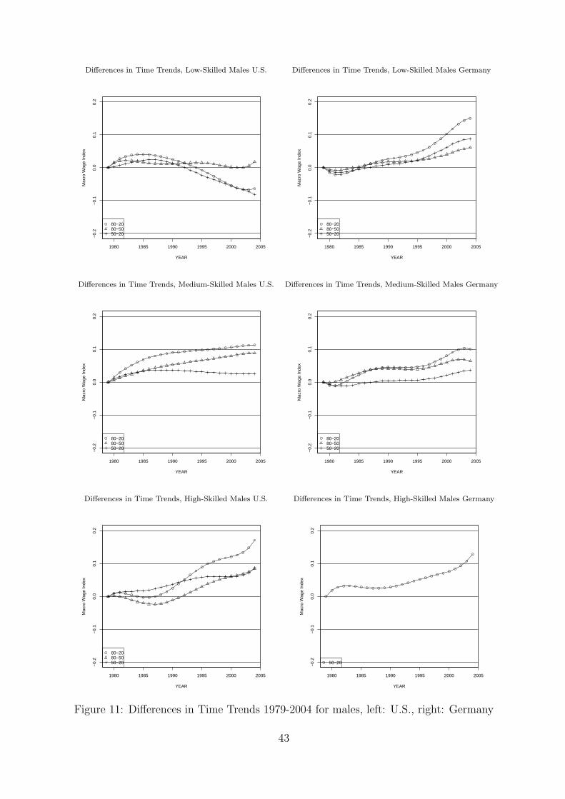
Differences in Time Trends, Low-Skilled Males U.S.

1980 1985 1990 1995 2000 2005

−0.

2−

0.1

0.0

0.1

0.2

YEAR

Mac

ro W

age

Inde

x

80−2080−5050−20

Differences in Time Trends, Low-Skilled Males Germany

1980 1985 1990 1995 2000 2005

−0.

2−

0.1

0.0

0.1

0.2

YEAR

Mac

ro W

age

Inde

x

80−2080−5050−20

Differences in Time Trends, Medium-Skilled Males U.S.

1980 1985 1990 1995 2000 2005

−0.

2−

0.1

0.0

0.1

0.2

YEAR

Mac

ro W

age

Inde

x

80−2080−5050−20

Differences in Time Trends, Medium-Skilled Males Germany

1980 1985 1990 1995 2000 2005

−0.

2−

0.1

0.0

0.1

0.2

YEAR

Mac

ro W

age

Inde

x

80−2080−5050−20

Differences in Time Trends, High-Skilled Males U.S.

1980 1985 1990 1995 2000 2005

−0.

2−

0.1

0.0

0.1

0.2

YEAR

Mac

ro W

age

Inde

x

80−2080−5050−20

Differences in Time Trends, High-Skilled Males Germany

1980 1985 1990 1995 2000 2005

−0.

2−

0.1

0.0

0.1

0.2

YEAR

Mac

ro W

age

Inde

x

50−20

Figure 11: Differences in Time Trends 1979-2004 for males, left: U.S., right: Germany

43

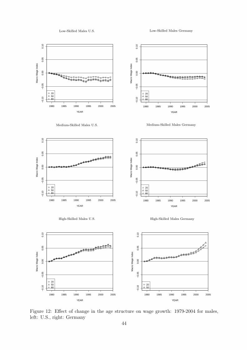
Low-Skilled Males U.S.

1980 1985 1990 1995 2000 2005

−0.

10−

0.05

0.00

0.05

0.10

YEAR

Mac

ro W

age

Inde

x

205080

Low-Skilled Males Germany

1980 1985 1990 1995 2000 2005

−0.

10−

0.05

0.00

0.05

0.10

YEAR

Mac

ro W

age

Inde

x

205080

Medium-Skilled Males U.S.

1980 1985 1990 1995 2000 2005

−0.

10−

0.05

0.00

0.05

0.10

YEAR

Mac

ro W

age

Inde

x

205080

Medium-Skilled Males Germany

1980 1985 1990 1995 2000 2005

−0.

10−

0.05

0.00

0.05

0.10

YEAR

Mac

ro W

age

Inde

x

205080

High-Skilled Males U.S.

1980 1985 1990 1995 2000 2005

−0.

10−

0.05

0.00

0.05

0.10

YEAR

Mac

ro W

age

Inde

x

205080

High-Skilled Males Germany

1980 1985 1990 1995 2000 2005

−0.

10−

0.05

0.00

0.05

0.10

YEAR

Mac

ro W

age

Inde

x

2050

Figure 12: Effect of change in the age structure on wage growth: 1979-2004 for males,left: U.S., right: Germany

44

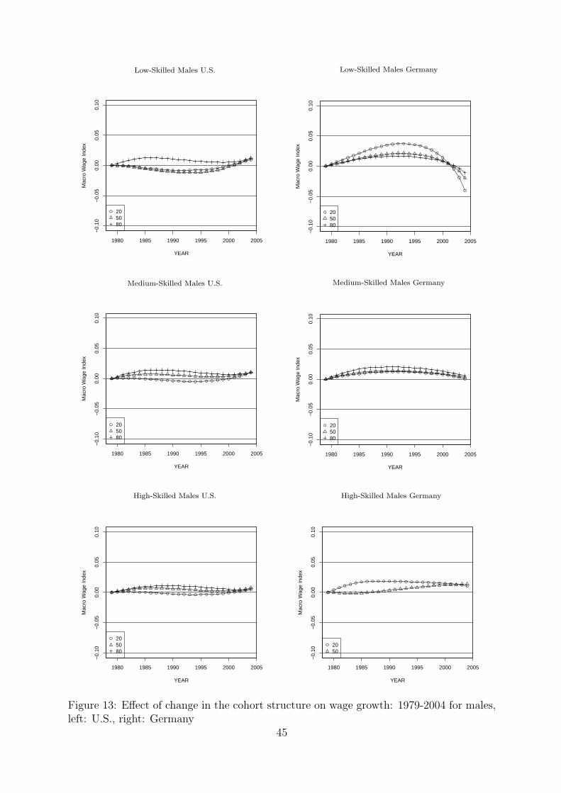
Low-Skilled Males U.S.

1980 1985 1990 1995 2000 2005

−0.

10−

0.05

0.00

0.05

0.10

YEAR

Mac

ro W

age

Inde

x

205080

Low-Skilled Males Germany

1980 1985 1990 1995 2000 2005

−0.

10−

0.05

0.00

0.05

0.10

YEAR

Mac

ro W

age

Inde

x

205080

Medium-Skilled Males U.S.

1980 1985 1990 1995 2000 2005

−0.

10−

0.05

0.00

0.05

0.10

YEAR

Mac

ro W

age

Inde

x

205080

Medium-Skilled Males Germany

1980 1985 1990 1995 2000 2005

−0.

10−

0.05

0.00

0.05

0.10

YEAR

Mac

ro W

age

Inde

x

205080

High-Skilled Males U.S.

1980 1985 1990 1995 2000 2005

−0.

10−

0.05

0.00

0.05

0.10

YEAR

Mac

ro W

age

Inde

x

205080

High-Skilled Males Germany

1980 1985 1990 1995 2000 2005

−0.

10−

0.05

0.00

0.05

0.10

YEAR

Mac

ro W

age

Inde

x

2050

Figure 13: Effect of change in the cohort structure on wage growth: 1979-2004 for males,left: U.S., right: Germany

45

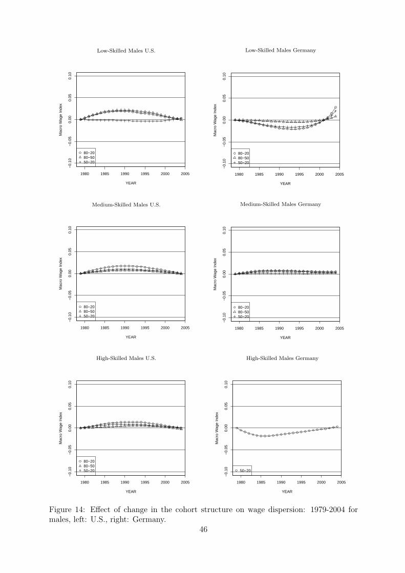
Low-Skilled Males U.S.

1980 1985 1990 1995 2000 2005

−0.

10−

0.05

0.00

0.05

0.10

YEAR

Mac

ro W

age

Inde

x

80−2080−5050−20

Low-Skilled Males Germany

1980 1985 1990 1995 2000 2005

−0.

10−

0.05

0.00

0.05

0.10

YEAR

Mac

ro W

age

Inde

x

80−2080−5050−20

Medium-Skilled Males U.S.

1980 1985 1990 1995 2000 2005

−0.

10−

0.05

0.00

0.05

0.10

YEAR

Mac

ro W

age

Inde

x

80−2080−5050−20

Medium-Skilled Males Germany

1980 1985 1990 1995 2000 2005

−0.

10−

0.05

0.00

0.05

0.10

YEAR

Mac

ro W

age

Inde

x

80−2080−5050−20

High-Skilled Males U.S.

1980 1985 1990 1995 2000 2005

−0.

10−

0.05

0.00

0.05

0.10

YEAR

Mac

ro W

age

Inde

x

80−2080−5050−20

High-Skilled Males Germany

1980 1985 1990 1995 2000 2005

−0.

10−

0.05

0.00

0.05

0.10

YEAR

Mac

ro W

age

Inde

x

50−20

Figure 14: Effect of change in the cohort structure on wage dispersion: 1979-2004 formales, left: U.S., right: Germany.

46

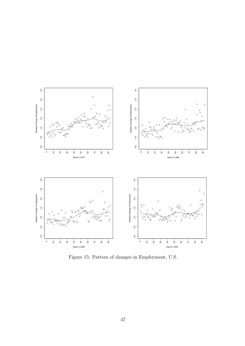
0.0

0.5

1.0

1.5

2.0

2.5

3.0

Rank in 1979

Rel

ativ

e C

hang

e of

Em

ploy

men

t

0 10 20 30 40 50 60 70 80 90

0.0

0.5

1.0

1.5

2.0

2.5

3.0

Rank in 1984

Rel

ativ

e C

hang

e of

Em

ploy

men

t

0 10 20 30 40 50 60 70 80 90

0.0

0.5

1.0

1.5

2.0

2.5

3.0

Rank in 1989

Rel

ativ

e C

hang

e of

Em

ploy

men

t

0 10 20 30 40 50 60 70 80 90

0.0

0.5

1.0

1.5

2.0

2.5

3.0

Rank in 1994

Rel

ativ

e C

hang

e of

Em

ploy

men

t

0 10 20 30 40 50 60 70 80 90

Figure 15: Pattern of changes in Employment, U.S.

47

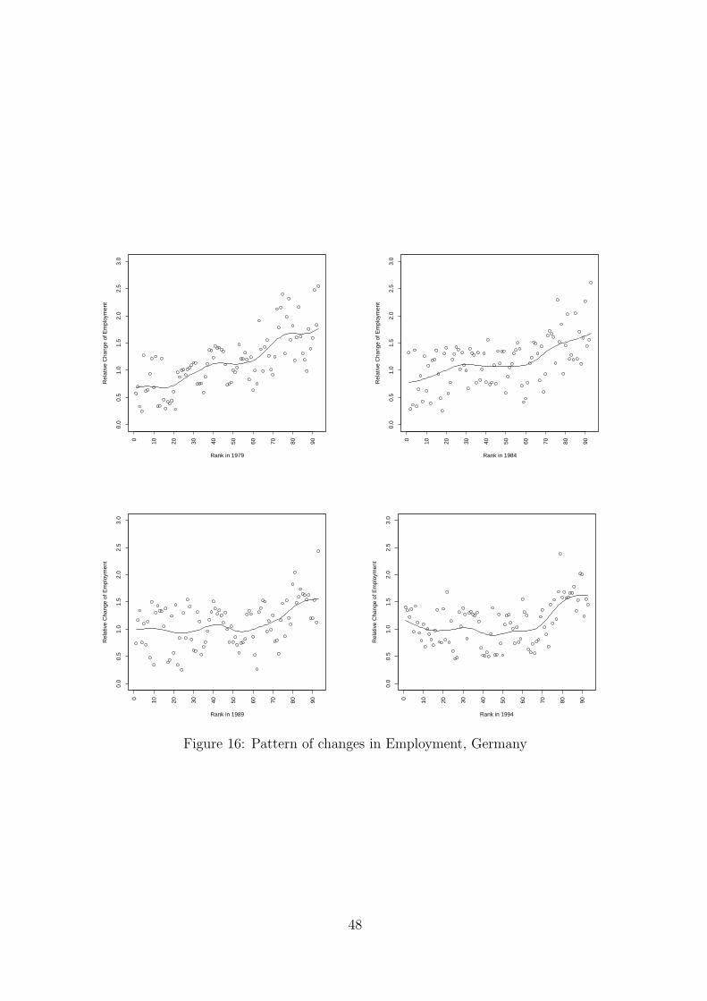
0.0

0.5

1.0

1.5

2.0

2.5

3.0

Rank in 1979

Rel

ativ

e C

hang

e of

Em

ploy

men

t

0 10 20 30 40 50 60 70 80 90

0.0

0.5

1.0

1.5

2.0

2.5

3.0

Rank in 1984

Rel

ativ

e C

hang

e of

Em

ploy

men

t

0 10 20 30 40 50 60 70 80 90

0.0

0.5

1.0

1.5

2.0

2.5

3.0

Rank in 1989

Rel

ativ

e C

hang

e of

Em

ploy

men

t

0 10 20 30 40 50 60 70 80 90

0.0

0.5

1.0

1.5

2.0

2.5

3.0

Rank in 1994

Rel

ativ

e C

hang

e of

Em

ploy

men

t

0 10 20 30 40 50 60 70 80 90

Figure 16: Pattern of changes in Employment, Germany

48