ABSTRACT

The objective of this paper is to examine the impact of unconventional monetary policy measures adopted in developed countries (the US, UK, Euro Area and Japan) on developing economies (Brazil, China, India and Russia). First, we analyse the domestic and cross-border financial market impact of unconventional monetary policy announcements by central banks, using a series of event stud-ies. We find that quantitative easing (QE) by the FED, BoE, ECB and BoJ influenced long term yields, equity prices, and possibly exchange rates both in the developed and developing countries (for example we find that QE resulted in decreases in long term yields by about 125 basis points in the US, about 100 basis points in the UK, and about 50 basis points in the Euro Area and Japan). Next, using the National Institute’s global macroeconomic model NIGEM, we conduct a series of macroeconomic simulations that allow us to assess the impact of lower yields, higher equity prices, and lower investment premia (attributable to unconventional monetary policy measures) on the real economy in the developed and developing countries (for example, we find that lower yields only, could have stimulated GDP (average change in levels, over a 5 year period) by about 1 /₄ per cent in the US, 1 /₂ per cent in the UK, /₄ per cent in the Euro Area and Japan, about 1 per cent in Brazil and Russia (in Brazil more than Russia), and /₄ per cent in India and China (in India more than China)).

JEL Classification: E58, F41, G15, C54

Keywords: unconventional monetary policy, international financial markets, open economy macro-economics, developed and developing countries, macroeconomic modelling.

DESA Working Paper No. 131ST/ESA/2013/DWP/131

October 2013

The spillover effects of unconventional monetary policies in major developed countries on developing countries

D e p a r t m e n t o f E c o n o m i c & S o c i a l A f f a i r s

Tatiana Fic*National Institute of Economic and Social Research

* I would like to thank Dawn Holland, Pingfan Hong, Ingo Pitterle, participants at the LINK Project conference at the United Nations, and research seminars at the NIESR and the Bank of England, for invaluable comments and discussions. Address for correspondence: tatianafic@hotmail.com

CONTENTS

Nontechnical summary . . . . . . . . . . . . . . . . . . . . . . . . . . . . . . . . . . . . . . . . . . . . . . . . . . . . . . . . 1

1 Introduction . . . . . . . . . . . . . . . . . . . . . . . . . . . . . . . . . . . . . . . . . . . . . . . . . . . . . . . . . . . . . . 2

2 Unconventional monetary policy in the US, UK, Euro Area, and Japan . . . . . . . . . . . . . . . 3

3 Spillover effects to Brazil, China, India and Russia . . . . . . . . . . . . . . . . . . . . . . . . . . . . . . . . 7

4 Methodology . . . . . . . . . . . . . . . . . . . . . . . . . . . . . . . . . . . . . . . . . . . . . . . . . . . . . . . . . . . . . 8

5 The impact of unconventional monetary policy on financial markets . . . . . . . . . . . . . . . . . 11

6 The impact of unconventional monetary policy on the real economy . . . . . . . . . . . . . . . . . 17

7 Exit strategy . . . . . . . . . . . . . . . . . . . . . . . . . . . . . . . . . . . . . . . . . . . . . . . . . . . . . . . . . . . . . . 21

Appendices

1 Event study and statistical analysis – details . . . . . . . . . . . . . . . . . . . . . . . . . . . . . . . . . . . . 25

2 A brief description of NIGEM . . . . . . . . . . . . . . . . . . . . . . . . . . . . . . . . . . . . . . . . . . . . . . . . 34

3 Macroeconomic simulations - details . . . . . . . . . . . . . . . . . . . . . . . . . . . . . . . . . . . . . . . . . . 36

UN/DESA Working Papers are preliminary documents circulated in a limited number of copies and posted on the DESA website at http://www.un.org/en/development/desa/papers/ to stimulate discussion and critical comment. The views and opinions expressed herein are those of the author and do not necessarily reflect those of the United Nations Secretariat. The designations and terminology employed may not conform to United Nations practice and do not imply the expression of any opinion whatsoever on the part of the Organization.

Typesetter: Rachel Babruskinas

UNITED NATIONS

Department of Economic and Social Affairs

UN Secretariat, 405 East 42nd Street

New York, N .Y . 10017, USA

e-mail: undesa@un .org

http://www .un .org/en/development/desa/papers/

Nontechnical summary

The objective of this paper is to examine the impact of unconventional monetary policies adopted in de-veloped countries – US, UK, Euro Area and Japan – on developing countries – Brazil, China, India and Russia. We adopt a two stage methodology. First we analyse the financial market impact of FED’s, ECB’s, BoE’s and BoJ’s announcements concern-ing unconventional monetary policy. We conduct a series of event studies and statistical analyses and look at the impacts of quantitative easing on long term yields, equity prices and exchange rates. Next, using the National Institute’s global macroeconomic model NIGEM we simulate the macroeconomic ef-fects of lower yields, higher equity prices, and lower investment premia (attributable to unconventional monetary policy) on the real economy in developed and developing countries.

Our key findings suggest that:

�� The scale of unconventional monetary policy measures adopted by the four major central banks, the FED, ECB, BoE and BoJ has been unprecedented. The size of central bank balance sheet has increased fivefold in the UK, fourfold in the US and it has doubled in the Euro Area and Japan.

�� The US and the UK have implemented very large quantitative easing programmes conduct-ed in three rounds in the US and two rounds in the UK. The scale of private and public asset purchases in the Euro Area has been somewhat smaller in relative terms. In Japan, the central bank had been pursuing quantitative easing pol-icy for some time before the crisis, and after the demise of the Lehman Brothers, the pace of asset purchases has increased, however, as compared to the other major central banks it has remained relatively moderate.

�� The FED’s and BoE’s QE programmes differed from those of the BoJ and the ECB in that they concentrated on bond purchases rather than on

direct lending to banks. The different tools re-flected different structures of these economies, with bond markets playing a relatively more im-portant role in the US and the UK, and banks playing a relatively more important role in conti-nental Europe and Japan.

�� The unconventional monetary policy has had a significant impact on the economies of the US, the UK, the Euro Area and Japan. Through channels such as global trade, global liquidity and global portfolio rebalancing, it has also had consequences for developing economies such as Brazil, China, India and Russia.

�� The impact of quantitative easing on the devel-oping economies has varied across countries, reflecting the scale of their exposure to the devel-oped countries (both in terms of trade and finan-cial linkages), their individual cyclical positions, and the type and scale of response of monetary authorities to capital inflows.

�� While the central bank unconventional inter-ventions have mitigated dysfunctions in targeted markets in the developed countries, they could have had spillover effects associated with inflows of capital and higher volatility in currency and financial markets in the developing countries.

�� Our event study analysis suggests that the quan-titative easing policy resulted in a decrease in long term yields by around 125 basis points in the US, 100 basis points in the UK and 50 basis points in the Euro Area and Japan. It may have also led to decreases in long term yields in the de-veloping economies – by about 175 basis points in Brazil, and about 25 basis points in China, India and Russia.

�� The quantitative easing policy has probably also contributed to increases in equity prices in the US, UK, the Euro Area, Brazil, China and India. The impact on equities in Japan and Russia may not have been that strong.

2 D E S A W O R K I N G P A P E R N O . 1 3 1

�� The event study analysis suggests that the quan-titative easing has not been accompanied by a major depreciation of the developed countries’ currencies (actually, the US dollar, the British pound and the Japanese yen have strengthened following major quantitative policy announce-ments). The quantitative easing has probably led to a relatively significant appreciation of the Brazilian real. The impact on other developing countries’ currencies has not been that strong (actually, the Indian rupee and the Russian ruble have depreciated).

�� While the impact of quantitative easing on the developing countries’ financial markets can be described as relatively significant, the impact on the real economy has been much smaller. This results from the smaller degree of financial devel-opment of these economies, and policy measures adopted by the domestic authorities to mitigate the effects of increased capital inflows.

�� Our macroeconomic scenario analysis shows that the impact of decreases in long term yields (coordinated scenario), among the developed economies, has had the biggest effect on the US, and the UK; among the developing countries - on Brazil (mainly through responsiveness of the Brazilian financial markets to FED’s QE an-nouncements) and Russia (mainly through trade linkages with Europe).

�� Allowing for additional effects coming from eq-uity prices and investment premia, the macroeco-nomic effects of quantitative easing are even big-ger, with the biggest effects among the developed economies materialising in the UK (mainly due to a stronger response of equity markets to QE announcements as compared to other countries), and among the developing economies - in Brazil.

�� In terms of an exit from unconventional mone-tary policy, the impacts on the developing econ-omies will depend on several factors: the scale of their exposure to the developed economies (both through trade and financial linkages); their cycli-cal position; the depth of their financial markets,

the scale of their external imbalances and the size of corporate and household debt; market senti-ment; and policy actions in the developing coun-tries aimed at mitigating the impact of increased capital outflows

�� The real effects of an exit can be limited for the developing economies, however, this is condi-tional on the behaviour of investors in bond markets, and, more generally, whether financial markets turbulence is avoided.

To recap, quantitative easing policies adopted in major developed countries have had a relatively significant impact on financial markets and the real economy locally. They have also had spillovers for developing countries’ financial markets, the impact on the real economy in the developing countries has probably been more muted.

1 Introduction

Since the global financial crisis, central banks have significantly expanded the set of their tools deployed to ensure financial stability and stimulate growth. These measures include: large scale purchases of gov-ernment bonds and private securities (quantitative easing), various lending programmes, and guidance over the future path of policy rates (Bean, 2012).

The objective of this paper is to examine the impact of unconventional monetary policy adopted in devel-oped countries on developing economies. The primary focus is on central bank balance sheet policies, and in particular quantitative easing measures. The uncon-ventional monetary policies introduced in major de-veloped countries have had an impact not only on the domestic economies, but they have also had interna-tional spillovers. Through global trade, global liquid-ity and global portfolio rebalancing, policy measures adopted in the developed countries have had an im-pact on the developing countries (Chen et al., 2013).

This paper adopts a two stage methodology to study the impact of unconventional monetary policies in developed countries on developing countries. We first

T H E S P I L L O V E R E F F E C T S O F U N C O N V E N T I O N A L M O N E T A R Y P O L I C I E S . . . 3

analyse the domestic and cross-border financial mar-ket impact of central bank announcements concern-ing unconventional monetary policy. We conduct a series of event studies and statistical analyses and look at the impact of quantitative easing by the FED, the BoE, the ECB and the BoJ on long term yields, equity prices, and exchange rates both in the US, UK, Euro Area and Japan, as well as in Brazil, China, India and Russia. Then, using the National Institute’s global macroeconomic model NIGEM, we conduct a series of macroeconomic simulations that allow us to assess the impact of lower yields, higher equity prices, and lower investment premia (attributable to quan-titative easing policy measures) on the real economy both in developed and developing countries.

The paper is organised as follows. First, we discuss unconventional monetary policy measures adopted by the major central banks – the Federal Reserve, the Bank of England, the European Central Bank and the Bank of Japan, and their potential spillover effects to the major developing economies: Brazil, China, India and Russia. Then, we study the impact of quantitative easing policy announcements by in-dividual central banks on financial markets in the developed and developing countries. We look at long term yields, equity prices, and exchange rates. Next, we simulate the effects of unconventional monetary policies (approximated by shocks to term premium,

equity premium and investment premium) on the real economy in the developed and developing coun-tries – the US, the UK, the Euro Area, Japan, Brazil, China, India, Russia. Finally, we discuss possible consequences of an exit from the unconventional monetary policy.

2 Unconventional monetarypolicy in the US, UK, Euro Area, and Japan

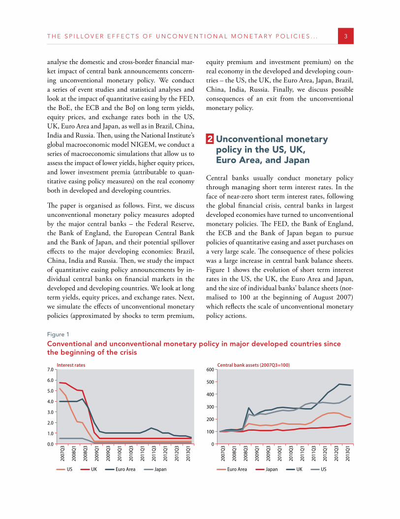
Central banks usually conduct monetary policy through managing short term interest rates. In the face of near-zero short term interest rates, following the global financial crisis, central banks in largest developed economies have turned to unconventional monetary policies. The FED, the Bank of England, the ECB and the Bank of Japan began to pursue policies of quantitative easing and asset purchases on a very large scale. The consequence of these policies was a large increase in central bank balance sheets. Figure 1 shows the evolution of short term interest rates in the US, the UK, the Euro Area and Japan, and the size of individual banks’ balance sheets (nor-malised to 100 at the beginning of August 2007) which reflects the scale of unconventional monetary policy actions.

Figure 1

Conventional and unconventional monetary policy in major developed countries since the beginning of the crisis

Interest rates

0.0

2.0

4.0

6.0

1.0

3.0

5.0

7.0Central bank assets (2007Q3=100)

0

100

300

500

200

400

600

2007

Q3

2008

Q1

2008

Q3

2009

Q1

2009

Q3

2010

Q1

2010

Q3

2011

Q1

2011

Q3

2012

Q1

2012

Q3

2013

Q1

US UK Euro Area Japan

2007

Q3

2008

Q1

2008

Q3

2009

Q1

2009

Q3

2010

Q1

2010

Q3

2011

Q1

2011

Q3

2012

Q1

2012

Q3

2013

Q1

Euro Area Japan UK US

4 D E S A W O R K I N G P A P E R N O . 1 3 1

Unconventional monetary policy measures adopted by the largest central banks included both direct asset purchases and various lending programmes. Initially, the quantitative easing (QE) programmes enacted by the largest central banks were to restore functioning of the dysfunctional financial markets; later the concern shifted to stimulating the econo-my. The details of balance sheet policies and quan-titative easing plans varied across central banks and depended on their specific motivations and different structures of the economy in individual countries. For example, the FED’s and BoE’s QE programmes differed from those of the BoJ and the ECB in that they concentrated on bond purchases rather than on direct lending to banks. The different tools reflected different structures of these economies, with bond markets playing a relatively more important role in the US and the UK, and banks playing a relatively more important role in continental Europe and Ja-pan (Fawley, Neely, 2013).

Below we briefly discuss unconventional monetary policy measures adopted by the Federal Reserve, the Bank of England, the European Central Bank and the Bank of Japan. The discussion is based on Fawley and Neely, 2013.

Federal Reserve

The US quantitative easing policy was conducted in three rounds. The first round, QE1, was announced from November 2008 to March 2009, and the tar-geted amount of assets to purchase oscillated around 1.725 trillion USD. In March 2011, the FED an-nounced a second round of QE, QE2, worth about 600 billion USD. It was followed by the Operation Twist, worth 667 billion USD, announced in Sep-tember 2011, and extended in February 2012. The QE3 programme was announced in September 2012. Unlike in the previous QE programmes, this time the FED committed to a pace of purchases rath-er than a total amount (40 billion USD per month; from December 2012, the programme was extended to 45 billion USD per month). On 19 June 2013, the FED announced a “tapering” of the QE policy, contingent upon continued positive economic data.

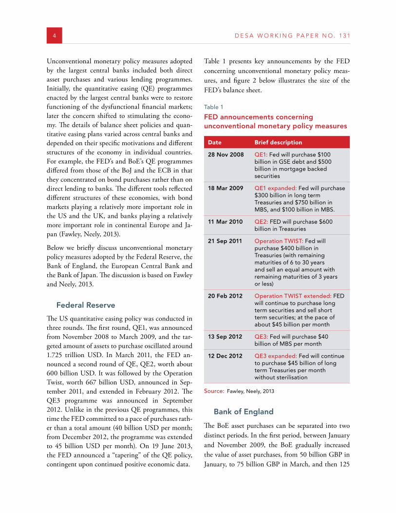
Table 1 presents key announcements by the FED concerning unconventional monetary policy meas-ures, and figure 2 below illustrates the size of the FED’s balance sheet.

Table 1

FED announcements concerning unconventional monetary policy measures

Date Brief description

28 Nov 2008 QE1: Fed will purchase $100 billion in GSE debt and $500 billion in mortgage backed securities

18 Mar 2009 QE1 expanded: Fed will purchase $300 billion in long term Treasuries and $750 billion in MBS, and $100 billion in MBS .

11 Mar 2010 QE2: FED will purchase $600 billion in Treasuries

21 Sep 2011 Operation TWIST: Fed will purchase $400 billion in Treasuries (with remaining maturities of 6 to 30 years and sell an equal amount with remaining maturities of 3 years or less)

20 Feb 2012 Operation TWIST extended: FED will continue to purchase long term securities and sell short term securities; at the pace of about $45 billion per month

13 Sep 2012 QE3: Fed will purchase $40 billion of MBS per month

12 Dec 2012 QE3 expanded: Fed will continue to purchase $45 billion of long term Treasuries per month without sterilisation

Source: Fawley, Neely, 2013

Bank of England

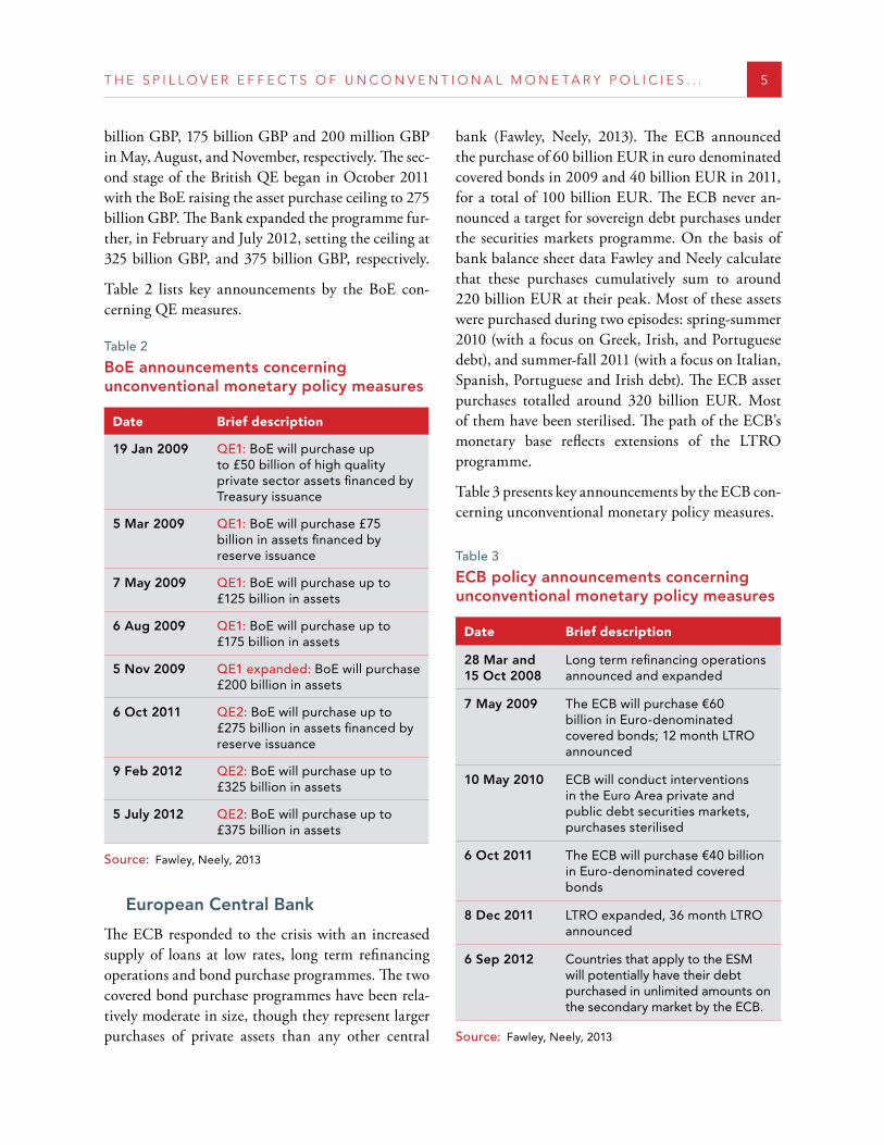
The BoE asset purchases can be separated into two distinct periods. In the first period, between January and November 2009, the BoE gradually increased the value of asset purchases, from 50 billion GBP in January, to 75 billion GBP in March, and then 125

T H E S P I L L O V E R E F F E C T S O F U N C O N V E N T I O N A L M O N E T A R Y P O L I C I E S . . . 5

billion GBP, 175 billion GBP and 200 million GBP in May, August, and November, respectively. The sec-ond stage of the British QE began in October 2011 with the BoE raising the asset purchase ceiling to 275 billion GBP. The Bank expanded the programme fur-ther, in February and July 2012, setting the ceiling at 325 billion GBP, and 375 billion GBP, respectively.

Table 2 lists key announcements by the BoE con-cerning QE measures.

Table 2

BoE announcements concerning unconventional monetary policy measures

Date Brief description

19 Jan 2009 QE1: BoE will purchase up to £50 billion of high quality private sector assets financed by Treasury issuance

5 Mar 2009 QE1: BoE will purchase £75 billion in assets financed by reserve issuance

7 May 2009 QE1: BoE will purchase up to £125 billion in assets

6 Aug 2009 QE1: BoE will purchase up to £175 billion in assets

5 Nov 2009 QE1 expanded: BoE will purchase £200 billion in assets

6 Oct 2011 QE2: BoE will purchase up to £275 billion in assets financed by reserve issuance

9 Feb 2012 QE2: BoE will purchase up to £325 billion in assets

5 July 2012 QE2: BoE will purchase up to £375 billion in assets

Source: Fawley, Neely, 2013

European Central Bank

The ECB responded to the crisis with an increased supply of loans at low rates, long term refinancing operations and bond purchase programmes. The two covered bond purchase programmes have been rela-tively moderate in size, though they represent larger purchases of private assets than any other central

bank (Fawley, Neely, 2013). The ECB announced the purchase of 60 billion EUR in euro denominated covered bonds in 2009 and 40 billion EUR in 2011, for a total of 100 billion EUR. The ECB never an-nounced a target for sovereign debt purchases under the securities markets programme. On the basis of bank balance sheet data Fawley and Neely calculate that these purchases cumulatively sum to around 220 billion EUR at their peak. Most of these assets were purchased during two episodes: spring-summer 2010 (with a focus on Greek, Irish, and Portuguese debt), and summer-fall 2011 (with a focus on Italian, Spanish, Portuguese and Irish debt). The ECB asset purchases totalled around 320 billion EUR. Most of them have been sterilised. The path of the ECB’s monetary base reflects extensions of the LTRO programme.

Table 3 presents key announcements by the ECB con-cerning unconventional monetary policy measures.

Table 3

ECB policy announcements concerning unconventional monetary policy measures

Date Brief description

28 Mar and 15 Oct 2008

Long term refinancing operations announced and expanded

7 May 2009 The ECB will purchase €60 billion in Euro-denominated covered bonds; 12 month LTRO announced

10 May 2010 ECB will conduct interventions in the Euro Area private and public debt securities markets, purchases sterilised

6 Oct 2011 The ECB will purchase €40 billion in Euro-denominated covered bonds

8 Dec 2011 LTRO expanded, 36 month LTRO announced

6 Sep 2012 Countries that apply to the ESM will potentially have their debt purchased in unlimited amounts on the secondary market by the ECB .

Source: Fawley, Neely, 2013

6 D E S A W O R K I N G P A P E R N O . 1 3 1

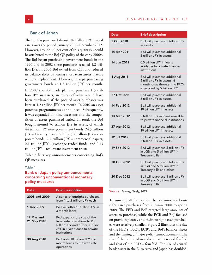
Bank of Japan

The BoJ has purchased almost 187 trillion JPY in total assets over the period January 2009-December 2012. However, around 40 per cent of this quantity should be attributed to the BoJ QE policy of the early 2000s. The BoJ began purchasing government bonds in the 1990 and in 2002 these purchases reached 1.2 tril-lion JPY. In 2006 BoJ exited from QE, and reduced its balance sheet by letting short term assets mature without replacement. However, it kept purchasing government bonds at 1.2 trillion JPY per month.

In 2009 the BoJ made plans to purchase 115 tril-lion JPY in assets, in excess of what would have been purchased, if the pace of asset purchases was kept at 1.2 trillion JPY per month. In 2010 an asset purchase programme was announced. Subsequently, it was expanded on nine occasions and the compo-sition of assets purchased varied. In total, the BoJ bought around 76 trillion JPY in assets, of which 44 trillion JPY were government bonds, 24.5 trillion JPY – Treasury discount bills, 3.2 trillion JPY – cor-porate bonds, 2.2 trillion JPY – commercial papers, 2.1 trillion JPY – exchange traded funds, and 0.13 trillion JPY – real estate investment trusts.

Table 4 lists key announcements concerning BoJ’s QE measures.

Table 4

Bank of Japan policy announcements concerning unconventional monetary policy measures

Date Brief description

2008 and 2009 A series of outright purchases, from 1 to 2 trillion JPY each

1 Dec 2009 BoJ will offer 10 trillion JPY in 3 month loans

17 Mar and 21 May 2010

BoJ expands the size of the fixed rate operations to 20 trillion JPY and offers 3 trillion JPY in 1-year loans to private institutions

30 Aug 2010 BoJ adds 10 trillion JPY in 6 month loans to thefixed rate operations

Date Brief description

5 Oct 2010 BoJ will purchase 5 trillion JPY in assets

14 Mar 2011 BoJ will purchase additional 5 trillion JPY in assets

14 Jun 2011 0 .5 trillion JPY in loans available to private financial institutions

4 Aug 2011 BoJ will purchase additional 5 trillion JPY in assets, 6 month lonas through the FROs expanded by 5 trillion JPY

27 Oct 2011 BoJ will purchase additional 5 trillion JPY in assets

14 Feb 2012 BoJ will purchase additional 10 trillion JPY in assets

13 Mar 2012 2 trillion JPY in loans available to private financial institutions

27 Apr 2012 BoJ will purchase additional 10 trillion JPY in assets

12 Jul 2012 BoJ will purchase additional 5 trillion JPY in assets

19 Sep 2012 BoJ will purchase 5 trillion JPY in JGB and 5 trillion JPY in Treasury bills

30 Oct 2012 BoJ will purchase 5 trillion JPY in JGB and 5 trillion JPY in Treasury bills and other

20 Dec 2012 BoJ will purchase 5 trillion JPY in JGB and 5 trillion JPY in Treasury bills

Source: Fawley, Neely, 2013

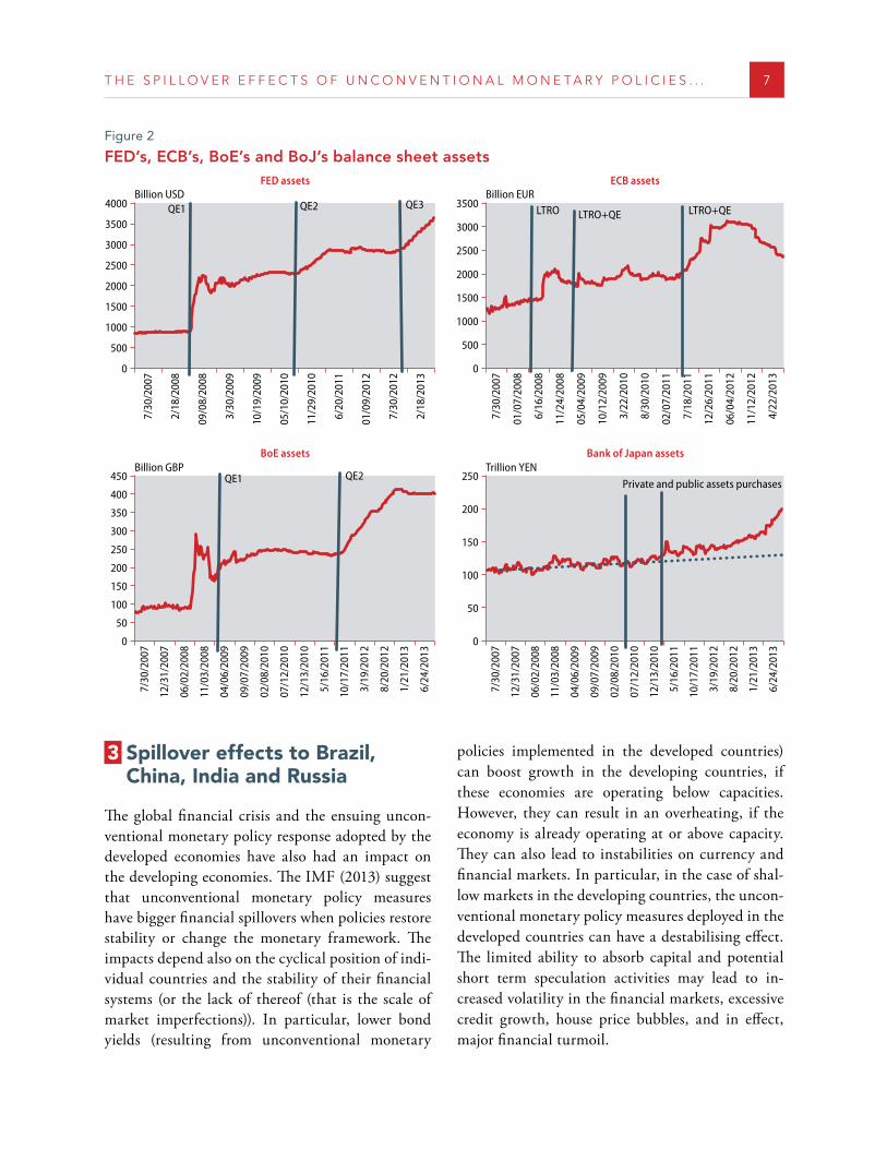
To sum up, all four central banks announced out-right asset purchases from autumn 2008 to spring 2009. The FED and BoE targeted large amounts of assets to purchase, while the ECB and BoJ focused on providing loans, and their outright asset purchas-es were relatively smaller. Figure 2 illustrates the size of the FED’s, BoE’s, ECB’s and BoJ’s balance sheets and the timing of major policy announcements. The size of the BoE’s balance sheet has increased fivefold and that of the FED – fourfold. The size of central bank assets in the Euro Area and Japan has doubled.

T H E S P I L L O V E R E F F E C T S O F U N C O N V E N T I O N A L M O N E T A R Y P O L I C I E S . . . 7

3 Spillover effects to Brazil,China, India and Russia

The global financial crisis and the ensuing uncon-ventional monetary policy response adopted by the developed economies have also had an impact on the developing economies. The IMF (2013) suggest that unconventional monetary policy measures have bigger financial spillovers when policies restore stability or change the monetary framework. The impacts depend also on the cyclical position of indi-vidual countries and the stability of their financial systems (or the lack of thereof (that is the scale of market imperfections)). In particular, lower bond yields (resulting from unconventional monetary

policies implemented in the developed countries) can boost growth in the developing countries, if these economies are operating below capacities. However, they can result in an overheating, if the economy is already operating at or above capacity. They can also lead to instabilities on currency and financial markets. In particular, in the case of shal-low markets in the developing countries, the uncon-ventional monetary policy measures deployed in the developed countries can have a destabilising effect. The limited ability to absorb capital and potential short term speculation activities may lead to in-creased volatility in the financial markets, excessive credit growth, house price bubbles, and in effect, major financial turmoil.

Figure 2

FED’s, ECB’s, BoE’s and BoJ’s balance sheet assetsFED assets

0

1000

2000

3500

3000

500

1500

2500

4000

ECB assets

0

1000

3000

2000

500

2500

1500

3500

BoE assets

0

100

200

400

50

150

300

350

250

450

Bank of Japan assets

0

100

200

50

150

250

7/30

/200

7

2/18

/200

8

09/0

8/20

08

3/30

/200

9

10/1

9/20

09

05/1

0/20

10

11/2

9/20

10

6/20

/201

1

01/0

9/20

12

7/30

/201

2

2/18

/201

3

Billion USD Billion EUR

Billion GBP

7/30

/200

7

12/3

1/20

07

06/0

2/20

08

11/0

3/20

08

04/0

6/20

09

09/0

7/20

09

02/0

8/20

10

07/1

2/20

10

12/1

3/20

10

5/16

/201

1

10/1

7/20

11

3/19

/201

2

8/20

/201

2

1/21

/201

3

6/24

/201

3

Trillion YEN

7/30

/200

7

12/3

1/20

07

06/0

2/20

08

11/0

3/20

08

04/0

6/20

09

09/0

7/20

09

02/0

8/20

10

07/1

2/20

10

12/1

3/20

10

5/16

/201

1

10/1

7/20

11

3/19

/201

2

8/20

/201

2

1/21

/201

3

6/24

/201

3

7/30

/200

7

01/0

7/20

08

6/16

/200

8

11/2

4/20

08

05/0

4/20

09

10/1

2/20

09

3/22

/201

0

8/30

/201

0

02/0

7/20

11

7/18

/201

1

12/2

6/20

11

06/0

4/20

12

11/1

2/20

12

4/22

/201

3

QE1 QE2 QE3 LTRO LTRO+QE LTRO+QE

QE1 QE2Private and public assets purchases

8 D E S A W O R K I N G P A P E R N O . 1 3 1

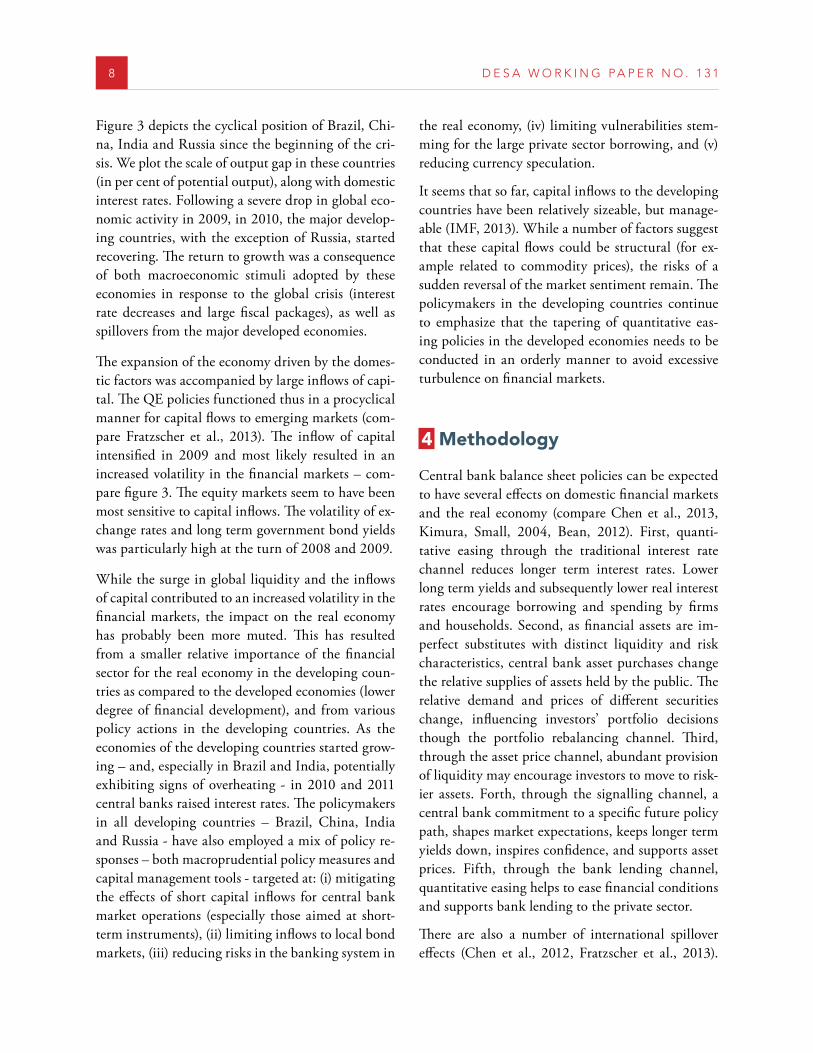
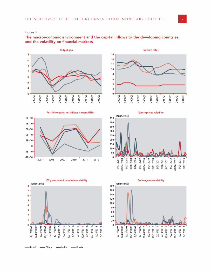
Figure 3 depicts the cyclical position of Brazil, Chi-na, India and Russia since the beginning of the cri-sis. We plot the scale of output gap in these countries (in per cent of potential output), along with domestic interest rates. Following a severe drop in global eco-nomic activity in 2009, in 2010, the major develop-ing countries, with the exception of Russia, started recovering. The return to growth was a consequence of both macroeconomic stimuli adopted by these economies in response to the global crisis (interest rate decreases and large fiscal packages), as well as spillovers from the major developed economies.

The expansion of the economy driven by the domes-tic factors was accompanied by large inflows of capi-tal. The QE policies functioned thus in a procyclical manner for capital flows to emerging markets (com-pare Fratzscher et al., 2013). The inflow of capital intensified in 2009 and most likely resulted in an increased volatility in the financial markets – com-pare figure 3. The equity markets seem to have been most sensitive to capital inflows. The volatility of ex-change rates and long term government bond yields was particularly high at the turn of 2008 and 2009.

While the surge in global liquidity and the inflows of capital contributed to an increased volatility in the financial markets, the impact on the real economy has probably been more muted. This has resulted from a smaller relative importance of the financial sector for the real economy in the developing coun-tries as compared to the developed economies (lower degree of financial development), and from various policy actions in the developing countries. As the economies of the developing countries started grow-ing – and, especially in Brazil and India, potentially exhibiting signs of overheating - in 2010 and 2011 central banks raised interest rates. The policymakers in all developing countries – Brazil, China, India and Russia - have also employed a mix of policy re-sponses – both macroprudential policy measures and capital management tools - targeted at: (i) mitigating the effects of short capital inflows for central bank market operations (especially those aimed at short-term instruments), (ii) limiting inflows to local bond markets, (iii) reducing risks in the banking system in

the real economy, (iv) limiting vulnerabilities stem-ming for the large private sector borrowing, and (v) reducing currency speculation.

It seems that so far, capital inflows to the developing countries have been relatively sizeable, but manage-able (IMF, 2013). While a number of factors suggest that these capital flows could be structural (for ex-ample related to commodity prices), the risks of a sudden reversal of the market sentiment remain. The policymakers in the developing countries continue to emphasize that the tapering of quantitative eas-ing policies in the developed economies needs to be conducted in an orderly manner to avoid excessive turbulence on financial markets.

4 Methodology

Central bank balance sheet policies can be expected to have several effects on domestic financial markets and the real economy (compare Chen et al., 2013, Kimura, Small, 2004, Bean, 2012). First, quanti-tative easing through the traditional interest rate channel reduces longer term interest rates. Lower long term yields and subsequently lower real interest rates encourage borrowing and spending by firms and households. Second, as financial assets are im-perfect substitutes with distinct liquidity and risk characteristics, central bank asset purchases change the relative supplies of assets held by the public. The relative demand and prices of different securities change, influencing investors’ portfolio decisions though the portfolio rebalancing channel. Third, through the asset price channel, abundant provision of liquidity may encourage investors to move to risk-ier assets. Forth, through the signalling channel, a central bank commitment to a specific future policy path, shapes market expectations, keeps longer term yields down, inspires confidence, and supports asset prices. Fifth, through the bank lending channel, quantitative easing helps to ease financial conditions and supports bank lending to the private sector.

There are also a number of international spillover effects (Chen et al., 2012, Fratzscher et al., 2013).

T H E S P I L L O V E R E F F E C T S O F U N C O N V E N T I O N A L M O N E T A R Y P O L I C I E S . . . 9

Figure 3

The macroeconomic environment and the capital inflows to the developing countries, and the volatility on financial markets

Output gap

-6

-4

0

6

4

-2

2

8

Interest rates

0

4

14

12

8

2

10

6

16

2007

Q3

2008

Q1

2008

Q3

2009

Q1

2009

Q3

2010

Q1

2010

Q3

2011

Q1

2011

Q3

2012

Q1

2012

Q3

2007

Q3

2008

Q1

2008

Q3

2009

Q1

2009

Q3

2010

Q1

2010

Q3

2011

Q1

2011

Q3

2012

Q1

2012

Q3

Brazil China India Russia

10Y government bond rates volatility

0

1

3

7

2

5

6

4

8

Exchange rate volatility

0

80

160

40

120

60

140

20

100

180Variance (%) Variance (%)

9/17

/200

7

02/0

4/20

08

6/23

/200

8

11/1

0/20

08

3/30

/200

9

8/17

/200

9

01/0

4/20

10

5/24

/201

0

10/1

1/20

10

2/28

/201

1

7/18

/201

1

12/0

5/20

11

4/23

/201

2

09/1

0/20

12

1/28

/201

3

6/17

/201

3

9/17

/200

7

02/0

4/20

08

6/23

/200

8

11/1

0/20

08

3/30

/200

9

8/17

/200

9

01/0

4/20

10

5/24

/201

0

10/1

1/20

10

2/28

/201

1

7/18

/201

1

12/0

5/20

11

4/23

/201

2

09/1

0/20

12

1/28

/201

3

6/17

/201

3

Portfolio equity, net inflows (current USD)

-2E+10

0

4E+10

-1E+10

2E+10

3E+10

1E+10

5E+10

Equity prices volatility

0

200

400

100

300

150

350

50

250

450Variance (%)

2007 2008 2009 2010 2011 2012

9/17

/200

7

02/0

4/20

08

6/23

/200

8

11/1

0/20

08

3/30

/200

9

8/17

/200

9

01/0

4/20

10

5/24

/201

0

10/1

1/20

10

2/28

/201

1

7/18

/201

1

12/0

5/20

11

4/23

/201

2

09/1

0/20

12

1/28

/201

3

6/17

/201

3

1 0 D E S A W O R K I N G P A P E R N O . 1 3 1

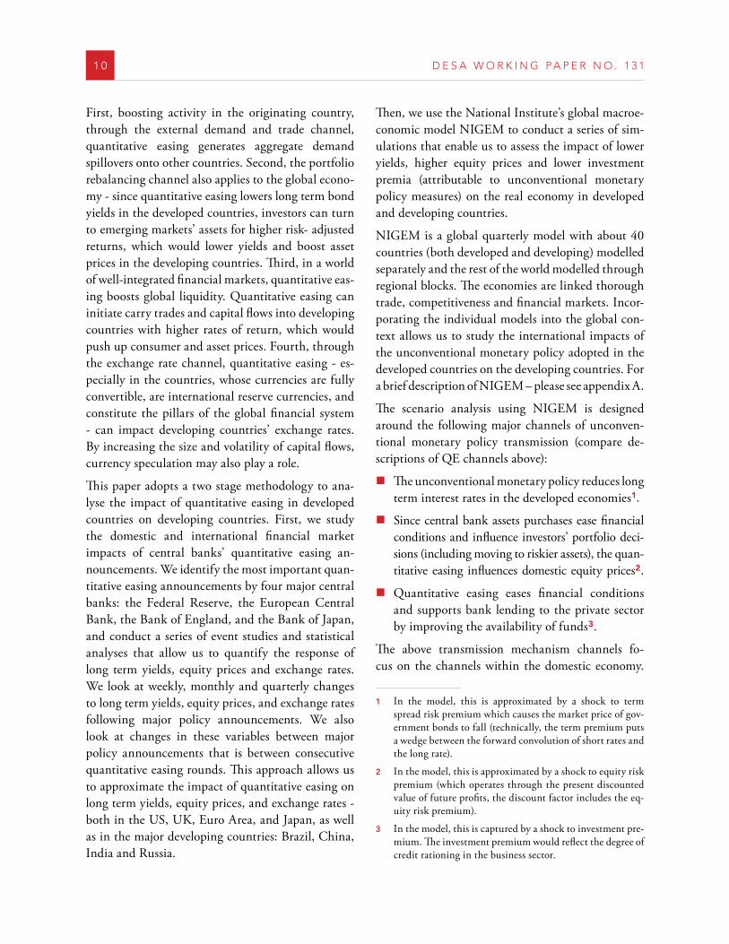
First, boosting activity in the originating country, through the external demand and trade channel, quantitative easing generates aggregate demand spillovers onto other countries. Second, the portfolio rebalancing channel also applies to the global econo-my - since quantitative easing lowers long term bond yields in the developed countries, investors can turn to emerging markets’ assets for higher risk- adjusted returns, which would lower yields and boost asset prices in the developing countries. Third, in a world of well-integrated financial markets, quantitative eas-ing boosts global liquidity. Quantitative easing can initiate carry trades and capital flows into developing countries with higher rates of return, which would push up consumer and asset prices. Fourth, through the exchange rate channel, quantitative easing - es-pecially in the countries, whose currencies are fully convertible, are international reserve currencies, and constitute the pillars of the global financial system - can impact developing countries’ exchange rates. By increasing the size and volatility of capital flows, currency speculation may also play a role.

This paper adopts a two stage methodology to ana-lyse the impact of quantitative easing in developed countries on developing countries. First, we study the domestic and international financial market impacts of central banks’ quantitative easing an-nouncements. We identify the most important quan-titative easing announcements by four major central banks: the Federal Reserve, the European Central Bank, the Bank of England, and the Bank of Japan, and conduct a series of event studies and statistical analyses that allow us to quantify the response of long term yields, equity prices and exchange rates. We look at weekly, monthly and quarterly changes to long term yields, equity prices, and exchange rates following major policy announcements. We also look at changes in these variables between major policy announcements that is between consecutive quantitative easing rounds. This approach allows us to approximate the impact of quantitative easing on long term yields, equity prices, and exchange rates - both in the US, UK, Euro Area, and Japan, as well as in the major developing countries: Brazil, China, India and Russia.

Then, we use the National Institute’s global macroe-conomic model NIGEM to conduct a series of sim-ulations that enable us to assess the impact of lower yields, higher equity prices and lower investment premia (attributable to unconventional monetary policy measures) on the real economy in developed and developing countries.

NIGEM is a global quarterly model with about 40 countries (both developed and developing) modelled separately and the rest of the world modelled through regional blocks. The economies are linked thorough trade, competitiveness and financial markets. Incor-porating the individual models into the global con-text allows us to study the international impacts of the unconventional monetary policy adopted in the developed countries on the developing countries. For a brief description of NIGEM – please see appendix A.

The scenario analysis using NIGEM is designed around the following major channels of unconven-tional monetary policy transmission (compare de-scriptions of QE channels above):

�� The unconventional monetary policy reduces long term interest rates in the developed economies1.

�� Since central bank assets purchases ease financial conditions and influence investors’ portfolio deci-sions (including moving to riskier assets), the quan-titative easing influences domestic equity prices2.

�� Quantitative easing eases financial conditions and supports bank lending to the private sector by improving the availability of funds3.

The above transmission mechanism channels fo-cus on the channels within the domestic economy.

1 In the model, this is approximated by a shock to term spread risk premium which causes the market price of gov-ernment bonds to fall (technically, the term premium puts a wedge between the forward convolution of short rates and the long rate).

2 In the model, this is approximated by a shock to equity risk premium (which operates through the present discounted value of future profits, the discount factor includes the eq-uity risk premium).

3 In the model, this is captured by a shock to investment pre-mium. The investment premium would reflect the degree of credit rationing in the business sector.

T H E S P I L L O V E R E F F E C T S O F U N C O N V E N T I O N A L M O N E T A R Y P O L I C I E S . . . 11

They allow us to study the impact of real effects of quantitative easing in the developed countries on the developing countries, which spread through

�� The traditional external demand and trade channels.

These channels are complemented by the following international channels:

�� The global portfolio rebalancing channel – in-vestors turn to emerging markets’ assets, which lowers yields and boosts asset prices4.

�� The global liquidity channel – an increase in global liquidity spurs capital inflows; it also eases financial conditions in the developing countries5.

To some extent, the international channels are simi-lar in nature to the domestic channels.

This paper uses several sources of data. The list of important quantitative easing policy announce-ments (dates and the volume of purchases) comes from Faweley and Neely (2013). Weekly data on long term yields (10 year government bond yields), equity prices (price indices NYSE, FTSE, DAX, FRC and NIKKEI) and bilateral exchange rates (BRL/USD, BRL/EUR, BRL/GBP, BRL/JPY, RMB/USD, RMB/EUR, RMB/GBP, RMB /JPY, INR/USD, INR/EUR, INR/GBP, INR/JPY, RUB/USD, RUB/EUR, RUB/GBP, RUB/JPY) used in the event study section come from Datastream. Weekly data on cen-tral bank assets come from individual central banks’ balance sheets. Quarterly macroeconomic data used in the simulations come from the NIGEM database. The period of analysis is 2007Q3 – 2013Q2.

5 The impact of unconventionalmonetary policy on financial markets

To assess the impact of unconventional monetary policy tools applied by the four largest central banks,

4 In the model this is approximated by a shock to long term yields in the developing countries

5 In the model this approximated by a shock to investment premium in the developing countries

on long term yields, equity prices and exchange rates in both developed and developing countries, we conduct a series of event studies combined with a statistical examination of the data.

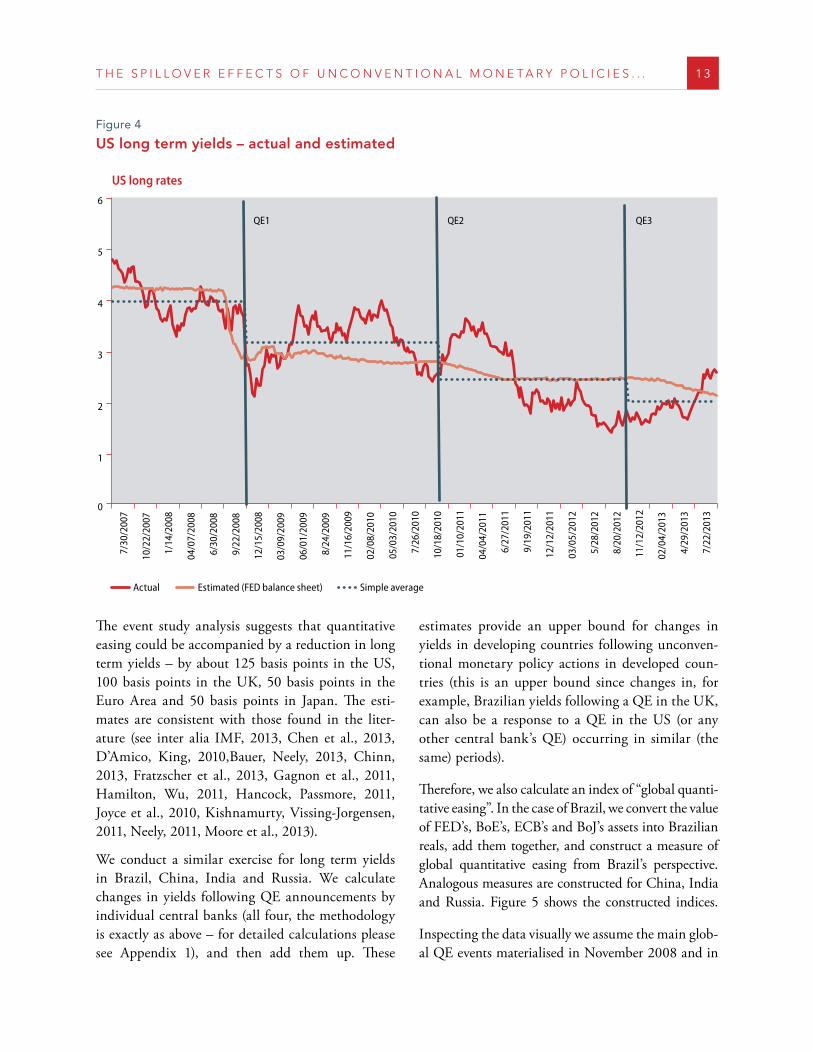
First, we study the impact of QE measures imple-mented by individual central banks on long term yields by looking at their weekly, monthly and quar-terly cumulative changes following important policy announcements6. Next, we look at changes in long term yields that materialised between consecutive rounds of quantitative easing. For example, in the case of the US, we compute average yields for the pe-riods Aug 2007 – Nov 2008 (before QE); Nov 2008 – Nov 2011 (QE1), Nov 2011-Sep 2012 (QE2), and from Sep 2012 onwards (QE3), and calculate differ-ences between them. We also estimate the relation-ship between long term yields and individual central banks’ assets7, and on the basis of this simple model calculate estimated yields, and look at changes in the estimated yields between consecutive QE rounds (for further details please see Appendix 1). Figure 4 pro-vides a graphical illustration for the US case.

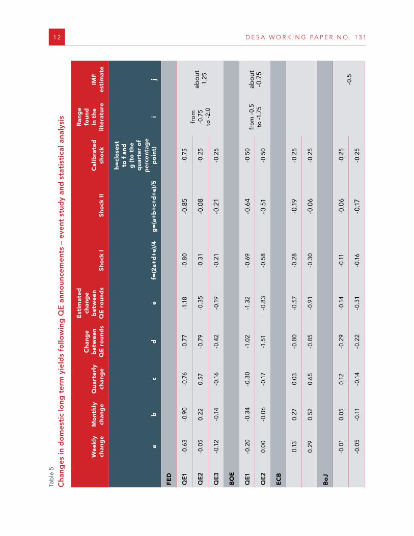
All changes in yields - weekly, monthly and quar-terly changes following QE policy announcements, as well as average changes between consecutive QE rounds, both actual and estimated, are shown in col-umns a-e in table 5. Columns f and g show algebraic combinations of the numbers reported in columns a-e, on the basis of which we calculate the size of possible shocks attributable to individual QE epi-sodes. We round the numbers obtained in columns f and g to the quarter of percentage point – they are presented in column h. For comparison, in columns i and j, we show estimates found in the literature.

6 Policy episodes investigated in the event study analysis: FED: QE1 – 25 Nov 2008, QE2 – 3 Nov 2010, QE3 12 Sep 2012, BoE: QE1 – 6 Feb, 5 Mar, 6 Aug, 5 Nov 2009, QE2 – 6 Oct 2011, 9 Feb 2012, ECB: 7 May 2009, 6 Oct 2011, BoJ: 30 Aug, 5 Oct 2010, and 14 Mar, 4 Aug 2011.

7 This simple regression should not in any case be interpreted in terms of a significant, full-fledged econometric estima-tion. It should be interpreted in terms of a simple statistical relationship (no causality). The relative weight of these esti-mates is not higher than that of simple weekly, monthly or quarterly changes following QE announcements.

12 D E S A W O R K I N G P A P E R N O . 1 3 1

Tab

le 5

Cha

nges

in d

om

esti

c lo

ng t

erm

yie

lds

follo

win

g Q

E a

nno

unce

men

ts –

eve

nt s

tud

y an

d s

tati

stic

al a

naly

sis

 W

eekl

y ch

ang

eM

ont

hly

chan

ge

Qua

rter

ly

chan

ge

Cha

nge

bet

wee

n Q

E r

oun

ds

Est

imat

ed

chan

ge

bet

wee

n Q

E r

oun

ds

Sho

ck I

Sho

ck I

IC

alib

rate

d

sho

ck

Ran

ge

foun

d

in t

he

liter

atur

eIM

F es

tim

ate

 a

bc

de

f=(2

a+d

+e)

/4g

=(a

+b

+c+

d+

e)/5

h=cl

ose

st

to f

and

g

(to

the

q

uart

er o

f p

erce

ntag

e p

oin

t)i

j

FED

QE1

-0 .6

3-0

.90

-0 .7

6-0

.77

-1 .1

8-0

.80

-0 .8

5-0

.75

fro

m

-0 .7

5 to

-2 .

0

abo

ut

-1 .2

5Q

E2

-0 .0

50 .

220 .

57-0

.79

-0 .3

5-0

.31

-0 .0

8-0

.25

QE

3-0

.12

-0 .1

4-0

.16

-0 .4

2-0

.19

-0 .2

1-0

.21

-0 .2

5

BO

E

QE1

-0 .2

0-0

.34

-0 .3

0-1

.02

-1 .3

2-0

.69

-0 .6

4-0

.50

fro

m -

0 .5

to -1

.75

abo

ut

-0 .7

5Q

E2

0 .0

0-0

.06

-0 .1

7-1

.51

-0 .8

3-0

.58

-0 .5

1-0

.50

EC

B

 0 .

130 .

270 .

03-0

.80

-0 .5

7-0

.28

-0 .1

9-0

.25

 0 .

290 .

520 .

65-0

.85

-0 .9

1-0

.30

-0 .0

6-0

.25

Bo

J

 -0

.01

0 .05

0 .12

-0 .2

9-0

.14

-0 .1

1-0

.06

-0 .2

5-0

.5 

-0 .0

5-0

.11

-0 .1

4-0

.22

-0 .3

1-0

.16

-0 .1

7-0

.25

T H E S P I L L O V E R E F F E C T S O F U N C O N V E N T I O N A L M O N E T A R Y P O L I C I E S . . . 13

The event study analysis suggests that quantitative easing could be accompanied by a reduction in long term yields – by about 125 basis points in the US, 100 basis points in the UK, 50 basis points in the Euro Area and 50 basis points in Japan. The esti-mates are consistent with those found in the liter-ature (see inter alia IMF, 2013, Chen et al., 2013, D’Amico, King, 2010,Bauer, Neely, 2013, Chinn, 2013, Fratzscher et al., 2013, Gagnon et al., 2011, Hamilton, Wu, 2011, Hancock, Passmore, 2011, Joyce et al., 2010, Kishnamurty, Vissing-Jorgensen, 2011, Neely, 2011, Moore et al., 2013).

We conduct a similar exercise for long term yields in Brazil, China, India and Russia. We calculate changes in yields following QE announcements by individual central banks (all four, the methodology is exactly as above – for detailed calculations please see Appendix 1), and then add them up. These

estimates provide an upper bound for changes in yields in developing countries following unconven-tional monetary policy actions in developed coun-tries (this is an upper bound since changes in, for example, Brazilian yields following a QE in the UK, can also be a response to a QE in the US (or any other central bank’s QE) occurring in similar (the same) periods).

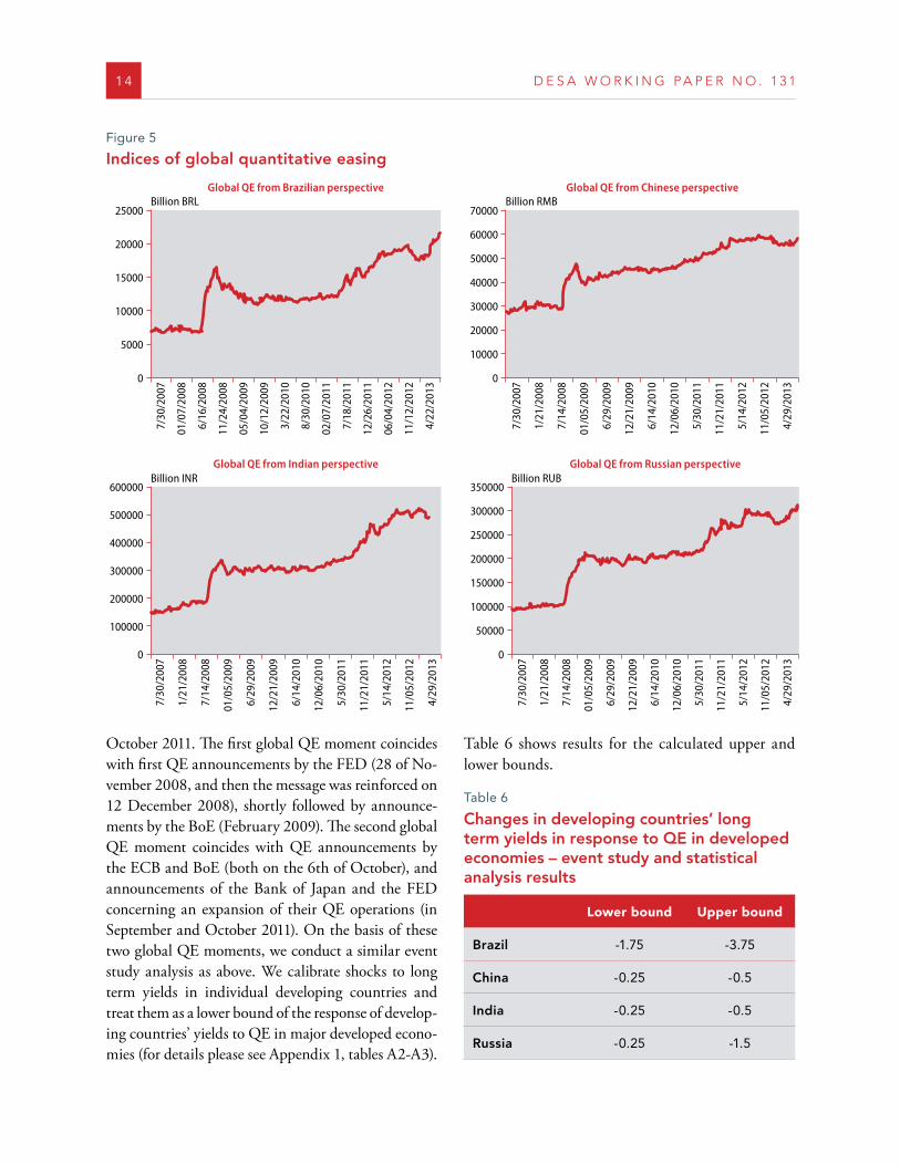
Therefore, we also calculate an index of “global quanti-tative easing”. In the case of Brazil, we convert the value of FED’s, BoE’s, ECB’s and BoJ’s assets into Brazilian reals, add them together, and construct a measure of global quantitative easing from Brazil’s perspective. Analogous measures are constructed for China, India and Russia. Figure 5 shows the constructed indices.

Inspecting the data visually we assume the main glob-al QE events materialised in November 2008 and in

Figure 4

US long term yields – actual and estimated

US long rates

0

2

5

4

1

3

6

7/30

/200

7

10/2

2/20

07

1/14

/200

8

04/0

7/20

08

6/30

/200

8

9/22

/200

8

12/1

5/20

08

03/0

9/20

09

06/0

1/20

09

8/24

/200

9

11/1

6/20

09

02/0

8/20

10

05/0

3/20

10

7/26

/201

0

10/1

8/20

10

01/1

0/20

11

04/0

4/20

11

6/27

/201

1

9/19

/201

1

12/1

2/20

11

03/0

5/20

12

5/28

/201

2

8/20

/201

2

11/1

2/20

12

02/0

4/20

13

4/29

/201

3

7/22

/201

3

Actual Estimated (FED balance sheet) Simple average

QE1 QE2 QE3

14 D E S A W O R K I N G P A P E R N O . 1 3 1

October 2011. The first global QE moment coincides with first QE announcements by the FED (28 of No-vember 2008, and then the message was reinforced on 12 December 2008), shortly followed by announce-ments by the BoE (February 2009). The second global QE moment coincides with QE announcements by the ECB and BoE (both on the 6th of October), and announcements of the Bank of Japan and the FED concerning an expansion of their QE operations (in September and October 2011). On the basis of these two global QE moments, we conduct a similar event study analysis as above. We calibrate shocks to long term yields in individual developing countries and treat them as a lower bound of the response of develop-ing countries’ yields to QE in major developed econo-mies (for details please see Appendix 1, tables A2-A3).

Table 6 shows results for the calculated upper and lower bounds.

Table 6

Changes in developing countries’ long term yields in response to QE in developed economies – event study and statistical analysis results

  Lower bound Upper bound

Brazil -1 .75 -3 .75

China -0 .25 -0 .5

India -0 .25 -0 .5

Russia -0 .25 -1 .5

Figure 5

Indices of global quantitative easing

Global QE from Brazilian perspective

0

5000

20000

15000

10000

25000

Global QE from Chinese perspective

0

20000

60000

40000

10000

50000

30000

70000

Global QE from Indian perspective

0

500000

100000

300000

400000

200000

600000

Global QE from Russian perspective

0

100000

300000

50000

200000

250000

150000

350000

Billion BRL Billion RMB

Billion INR Billion RUB

7/30

/200

7

01/0

7/20

08

6/16

/200

8

11/2

4/20

08

05/0

4/20

09

10/1

2/20

09

3/22

/201

0

8/30

/201

0

02/0

7/20

11

7/18

/201

1

12/2

6/20

11

06/0

4/20

12

11/1

2/20

12

4/22

/201

3

7/30

/200

7

1/21

/200

8

7/14

/200

8

01/0

5/20

09

6/29

/200

9

12/2

1/20

09

6/14

/201

0

12/0

6/20

10

5/30

/201

1

11/2

1/20

11

5/14

/201

2

11/0

5/20

12

4/29

/201

3

7/30

/200

7

1/21

/200

8

7/14

/200

8

01/0

5/20

09

6/29

/200

9

12/2

1/20

09

6/14

/201

0

12/0

6/20

10

5/30

/201

1

11/2

1/20

11

5/14

/201

2

11/0

5/20

12

4/29

/201

3

7/30

/200

7

1/21

/200

8

7/14

/200

8

01/0

5/20

09

6/29

/200

9

12/2

1/20

09

6/14

/201

0

12/0

6/20

10

5/30

/201

1

11/2

1/20

11

5/14

/201

2

11/0

5/20

12

4/29

/201

3

T H E S P I L L O V E R E F F E C T S O F U N C O N V E N T I O N A L M O N E T A R Y P O L I C I E S . . . 15

The event study analysis suggests that central bank balance sheet policies probably led to a reduction in long term yields in the developing countries. The ef-fects seem to be strongest in the case of Brazil, where long term interest rates dropped by 175 basis points (and possibly more). The reaction of long term yields in China, India and Russia was softer – it is likely that the yields decreased by not more than 25 basis points.

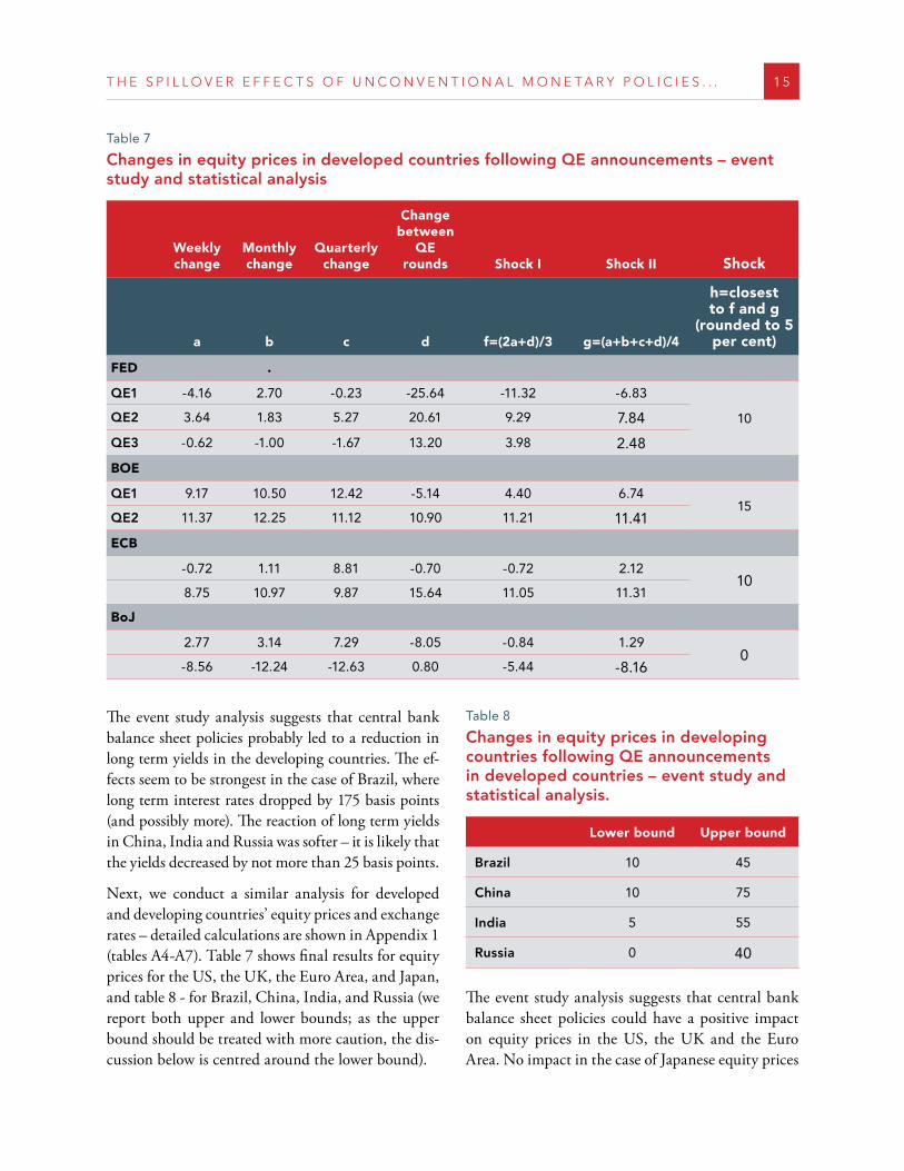
Next, we conduct a similar analysis for developed and developing countries’ equity prices and exchange rates – detailed calculations are shown in Appendix 1 (tables A4-A7). Table 7 shows final results for equity prices for the US, the UK, the Euro Area, and Japan, and table 8 - for Brazil, China, India, and Russia (we report both upper and lower bounds; as the upper bound should be treated with more caution, the dis-cussion below is centred around the lower bound).

Table 8

Changes in equity prices in developing countries following QE announcements in developed countries – event study and statistical analysis.

  Lower bound Upper bound

Brazil 10 45

China 10 75

India 5 55

Russia 0 40

The event study analysis suggests that central bank balance sheet policies could have a positive impact on equity prices in the US, the UK and the Euro Area. No impact in the case of Japanese equity prices

Table 7

Changes in equity prices in developed countries following QE announcements – event study and statistical analysis

 

Weekly change

Monthly change

Quarterly change

Change between

QE rounds Shock I Shock II Shock

  a b c d f=(2a+d)/3 g=(a+b+c+d)/4

h=closest to f and g

(rounded to 5 per cent)

FED   .          

QE1 -4 .16 2 .70 -0 .23 -25 .64 -11 .32 -6 .83

10QE2 3 .64 1 .83 5 .27 20 .61 9 .29 7 .84

QE3 -0 .62 -1 .00 -1 .67 13 .20 3 .98 2 .48

BOE              

QE1 9 .17 10 .50 12 .42 -5 .14 4 .40 6 .7415

QE2 11 .37 12 .25 11 .12 10 .90 11 .21 11 .41

ECB              

-0 .72 1 .11 8 .81 -0 .70 -0 .72 2 .1210

8 .75 10 .97 9 .87 15 .64 11 .05 11 .31

BoJ            

  2 .77 3 .14 7 .29 -8 .05 -0 .84 1 .290

  -8 .56 -12 .24 -12 .63 0 .80 -5 .44 -8 .16

16 D E S A W O R K I N G P A P E R N O . 1 3 1

was found8. It is possible, that equity markets in the UK were somewhat more responsive to QE than eq-uity markets in the US, and the Euro Area.

In the case of the developing countries, the most sig-nificant effects seem to have materialised in Brazil, China and India. The Russian equity markets prob-ably remained less responsive to QE in the major developed economies.

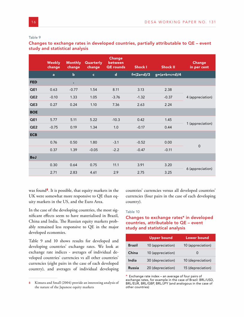
Table 9 and 10 shows results for developed and developing countries’ exchange rates. We look at exchange rate indices - averages of individual de-veloped countries’ currencies vs all other countries’ currencies (eight pairs in the case of each developed country), and averages of individual developing

8 Kimura and Small (2004) provide an interesting analysis of the nature of the Japanese equity markets

countries’ currencies versus all developed countries’ currencies (four pairs in the case of each developing country).

Table 10

Changes to exchange rates* in developed countries, attributable to QE – event study and statistical analysis

  Upper bound Lower bound

Brazil 10 (appreciation) 10 (appreciation)

China 10 (appreciation) 0

India 30 (depreciation) 10 (depreciation)

Russia 20 (depreciation) 15 (depreciation)

* Exchange rate index – an average of four pairs of exchange rates, for example in the case of Brazil: BRL/USD, BRL/EUR, BRL/GBP, BRL/JPY (and analogous in the case of other countries)

Table 9

Changes to exchange rates in developed countries, partially attributable to QE – event study and statistical analysis

 Weekly change

Monthly change

Quarterly change

Change between

QE rounds Shock I Shock IIChange

in per cent

  a b c d f=(2a+d)/3 g=(a+b+c+d)/4  

FED   .          

QE1 0 .63 -0 .77 1 .54 8 .11 3 .13 2 .38

4 (appreciation)QE2 -0 .10 1 .33 1 .05 -3 .76 -1 .32 -0 .37

QE3 0 .27 0 .24 1 .10 7 .36 2 .63 2 .24

BOE              

QE1 5 .77 5 .11 5 .22 -10 .3 0 .42 1 .451 (appreciation)

QE2 -0 .75 0 .19 1 .34 1 .0 -0 .17 0 .44

ECB            

  0 .76 0 .50 1 .80 -3 .1 -0 .52 0 .000

  0 .37 1 .39 -0 .05 -2 .2 -0 .47 -0 .11

BoJ              

  0 .30 0 .64 0 .75 11 .1 3 .91 3 .206 (appreciation)

  2 .71 2 .83 4 .61 2 .9 2 .75 3 .25

T H E S P I L L O V E R E F F E C T S O F U N C O N V E N T I O N A L M O N E T A R Y P O L I C I E S . . . 17

The event study analysis suggests that expansionary central bank balance sheet policies in the developed countries did not result in major depreciations of their currencies. On the contrary, the US dollar9, the Japanese yen, and possibly the UK pound gained strength following QE announcements, in line with the safe heavens hypothesis. The quantitative easing policies probably led to an appreciation of the Bra-zilian real.

6 The impact of unconventionalmonetary policy on the real economy

On the basis of calibrated shocks to long term yields and equity prices, and to investment premium, all of which can be attributed to unconventional mon-etary policy, we conduct a series of macroeconomic simulations, and try to assess the impact of uncon-ventional monetary policy on the real economy in developed and developing countries.

We analyse the following scenarios:

�� Uncoordinated scenarios: we look at the effects of unconventional monetary policies in the US, the UK, the Euro Area and Japan separately, that is in isolation from each other.

�� Coordinated scenario: we analyse the impacts of a joint scenario, where all major central banks - FED, ECB, BoJ, and BoE - adopt QE simul-taneously; moreover, we assume, that there is an immediate reaction of financial markets in developing countries – Brazil, China, India and Russia.

Uncoordinated scenarios

We simulate the macroeconomic impacts of central bank balance sheet policies adopted in the US, the UK, the Euro Area and Japan. We assume that the

9 While QE1 and QE3 were accompanied by an appreciation of the US currency, QE2 could led to a minor depreciation.

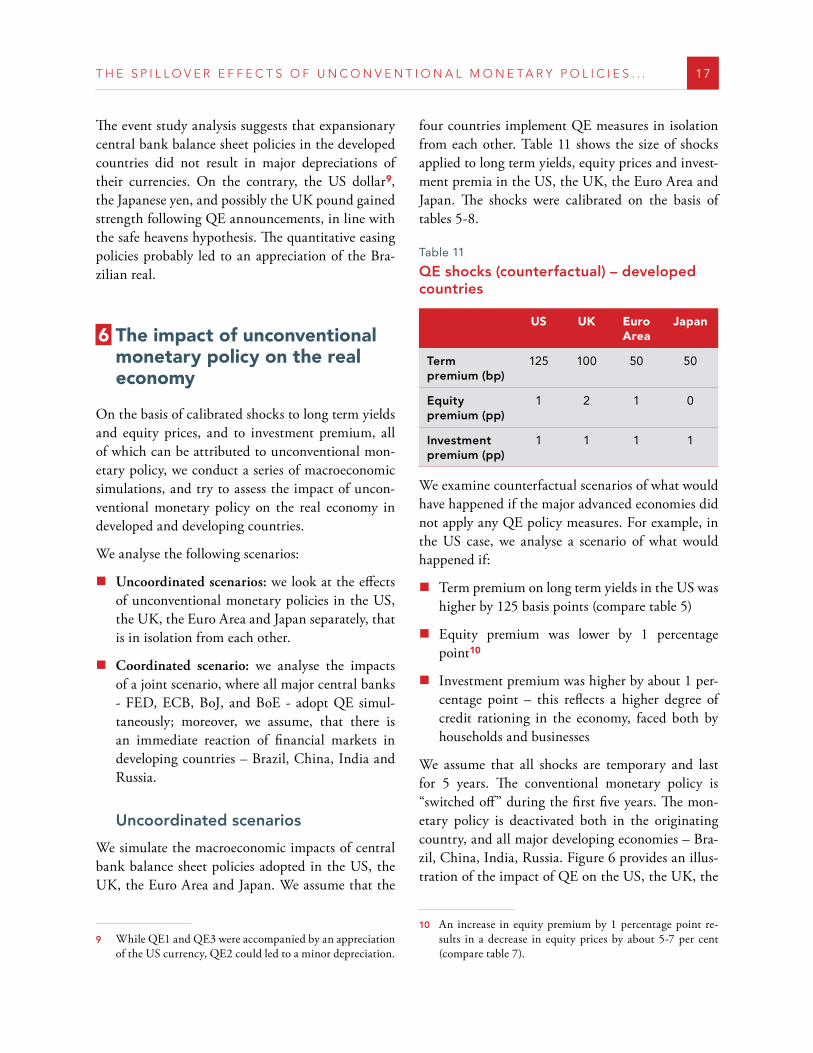
four countries implement QE measures in isolation from each other. Table 11 shows the size of shocks applied to long term yields, equity prices and invest-ment premia in the US, the UK, the Euro Area and Japan. The shocks were calibrated on the basis of tables 5-8.

Table 11

QE shocks (counterfactual) – developed countries

  US UK Euro Area

Japan

Term premium (bp)

125 100 50 50

Equity premium (pp)

1 2 1 0

Investment premium (pp)

1 1 1 1

We examine counterfactual scenarios of what would have happened if the major advanced economies did not apply any QE policy measures. For example, in the US case, we analyse a scenario of what would happened if:

�� Term premium on long term yields in the US was higher by 125 basis points (compare table 5)

�� Equity premium was lower by 1 percentage point10

�� Investment premium was higher by about 1 per-centage point – this reflects a higher degree of credit rationing in the economy, faced both by households and businesses

We assume that all shocks are temporary and last for 5 years. The conventional monetary policy is “switched off” during the first five years. The mon-etary policy is deactivated both in the originating country, and all major developing economies – Bra-zil, China, India, Russia. Figure 6 provides an illus-tration of the impact of QE on the US, the UK, the

10 An increase in equity premium by 1 percentage point re-sults in a decrease in equity prices by about 5-7 per cent (compare table 7).

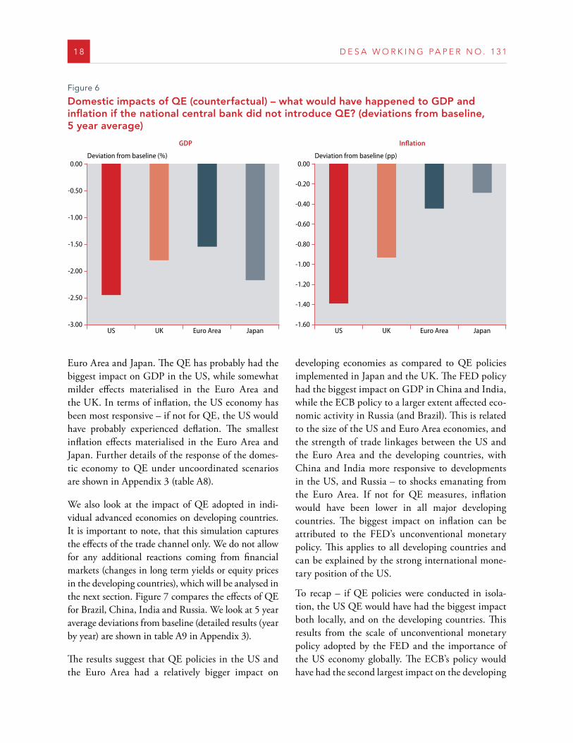
18 D E S A W O R K I N G P A P E R N O . 1 3 1

Euro Area and Japan. The QE has probably had the biggest impact on GDP in the US, while somewhat milder effects materialised in the Euro Area and the UK. In terms of inflation, the US economy has been most responsive – if not for QE, the US would have probably experienced deflation. The smallest inflation effects materialised in the Euro Area and Japan. Further details of the response of the domes-tic economy to QE under uncoordinated scenarios are shown in Appendix 3 (table A8).

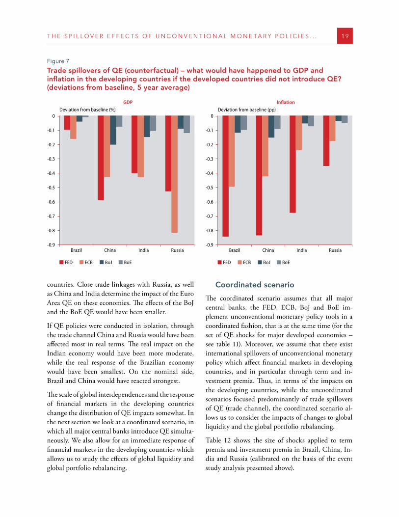
We also look at the impact of QE adopted in indi-vidual advanced economies on developing countries. It is important to note, that this simulation captures the effects of the trade channel only. We do not allow for any additional reactions coming from financial markets (changes in long term yields or equity prices in the developing countries), which will be analysed in the next section. Figure 7 compares the effects of QE for Brazil, China, India and Russia. We look at 5 year average deviations from baseline (detailed results (year by year) are shown in table A9 in Appendix 3).

The results suggest that QE policies in the US and the Euro Area had a relatively bigger impact on

developing economies as compared to QE policies implemented in Japan and the UK. The FED policy had the biggest impact on GDP in China and India, while the ECB policy to a larger extent affected eco-nomic activity in Russia (and Brazil). This is related to the size of the US and Euro Area economies, and the strength of trade linkages between the US and the Euro Area and the developing countries, with China and India more responsive to developments in the US, and Russia – to shocks emanating from the Euro Area. If not for QE measures, inflation would have been lower in all major developing countries. The biggest impact on inflation can be attributed to the FED’s unconventional monetary policy. This applies to all developing countries and can be explained by the strong international mone-tary position of the US.

To recap – if QE policies were conducted in isola-tion, the US QE would have had the biggest impact both locally, and on the developing countries. This results from the scale of unconventional monetary policy adopted by the FED and the importance of the US economy globally. The ECB’s policy would have had the second largest impact on the developing

Figure 6

Domestic impacts of QE (counterfactual) – what would have happened to GDP and inflation if the national central bank did not introduce QE? (deviations from baseline, 5 year average)

GDP

-3.00

-2.00

-0.50

-2.50

-1.50

0.00

-1.00

Inflation

-1.60

-1.40

-0.80

-0.20

-1.20

-0.40

-1.00

0.00

-0.60

US UK Euro Area Japan Euro Area JapanUKUS

Deviation from baseline (%) Deviation from baseline (pp)

T H E S P I L L O V E R E F F E C T S O F U N C O N V E N T I O N A L M O N E T A R Y P O L I C I E S . . . 19

countries. Close trade linkages with Russia, as well as China and India determine the impact of the Euro Area QE on these economies. The effects of the BoJ and the BoE QE would have been smaller.

If QE policies were conducted in isolation, through the trade channel China and Russia would have been affected most in real terms. The real impact on the Indian economy would have been more moderate, while the real response of the Brazilian economy would have been smallest. On the nominal side, Brazil and China would have reacted strongest.

The scale of global interdependences and the response of financial markets in the developing countries change the distribution of QE impacts somewhat. In the next section we look at a coordinated scenario, in which all major central banks introduce QE simulta-neously. We also allow for an immediate response of financial markets in the developing countries which allows us to study the effects of global liquidity and global portfolio rebalancing.

Coordinated scenario

The coordinated scenario assumes that all major central banks, the FED, ECB, BoJ and BoE im-plement unconventional monetary policy tools in a coordinated fashion, that is at the same time (for the set of QE shocks for major developed economies – see table 11). Moreover, we assume that there exist international spillovers of unconventional monetary policy which affect financial markets in developing countries, and in particular through term and in-vestment premia. Thus, in terms of the impacts on the developing countries, while the uncoordinated scenarios focused predominantly of trade spillovers of QE (trade channel), the coordinated scenario al-lows us to consider the impacts of changes to global liquidity and the global portfolio rebalancing.

Table 12 shows the size of shocks applied to term premia and investment premia in Brazil, China, In-dia and Russia (calibrated on the basis of the event study analysis presented above).

Figure 7

Trade spillovers of QE (counterfactual) – what would have happened to GDP and inflation in the developing countries if the developed countries did not introduce QE? (deviations from baseline, 5 year average)

GDP

-0.9

-0.6

-0.1

-0.8

-0.4

0

-0.2

-0.7

-0.5

-0.3

-0.9

-0.6

-0.1

-0.8

-0.4

0

-0.2

-0.7

-0.5

-0.3

Inflation

Brazil China India Russia India RussiaChinaBrazil

Deviation from baseline (%) Deviation from baseline (pp)

FED ECB BoJ BoE FED ECB BoJ BoE

2 0 D E S A W O R K I N G P A P E R N O . 1 3 1

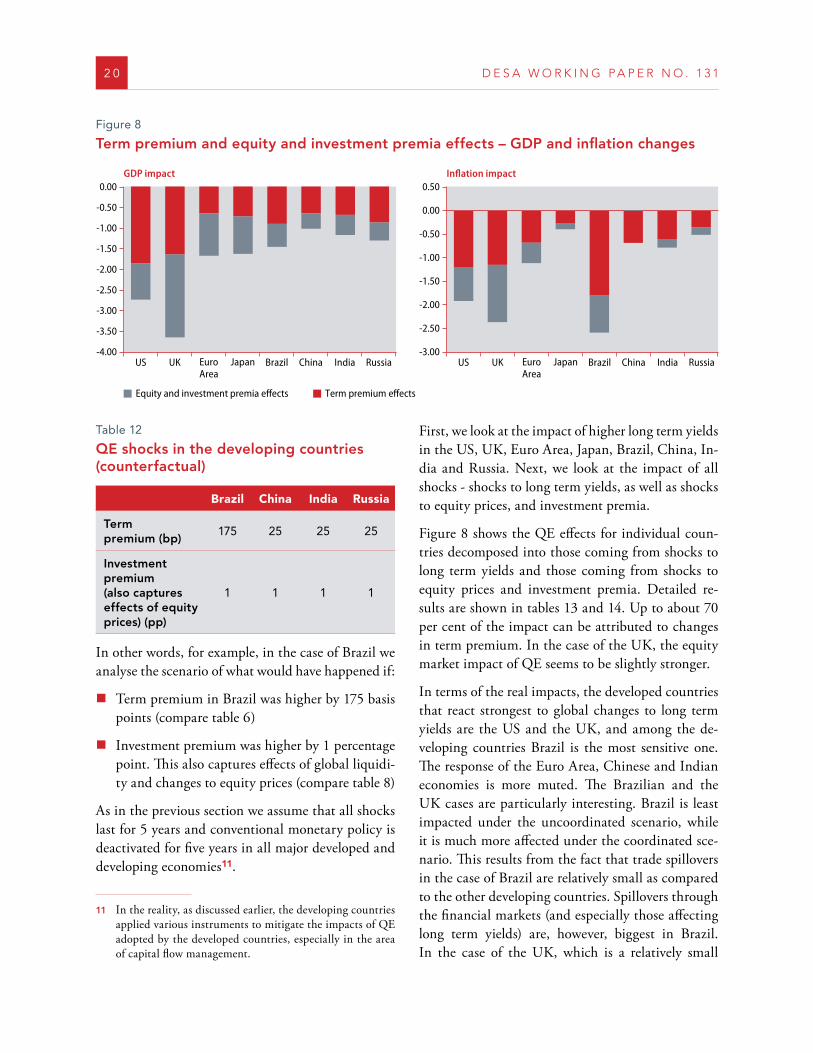
Table 12

QE shocks in the developing countries (counterfactual)

  Brazil China India Russia

Term premium (bp)

175 25 25 25

Investment premium (also captures effects of equity prices) (pp)

1 1 1 1

In other words, for example, in the case of Brazil we analyse the scenario of what would have happened if:

�� Term premium in Brazil was higher by 175 basis points (compare table 6)

�� Investment premium was higher by 1 percentage point. This also captures effects of global liquidi-ty and changes to equity prices (compare table 8)

As in the previous section we assume that all shocks last for 5 years and conventional monetary policy is deactivated for five years in all major developed and developing economies11.

11 In the reality, as discussed earlier, the developing countries applied various instruments to mitigate the impacts of QE adopted by the developed countries, especially in the area of capital flow management.

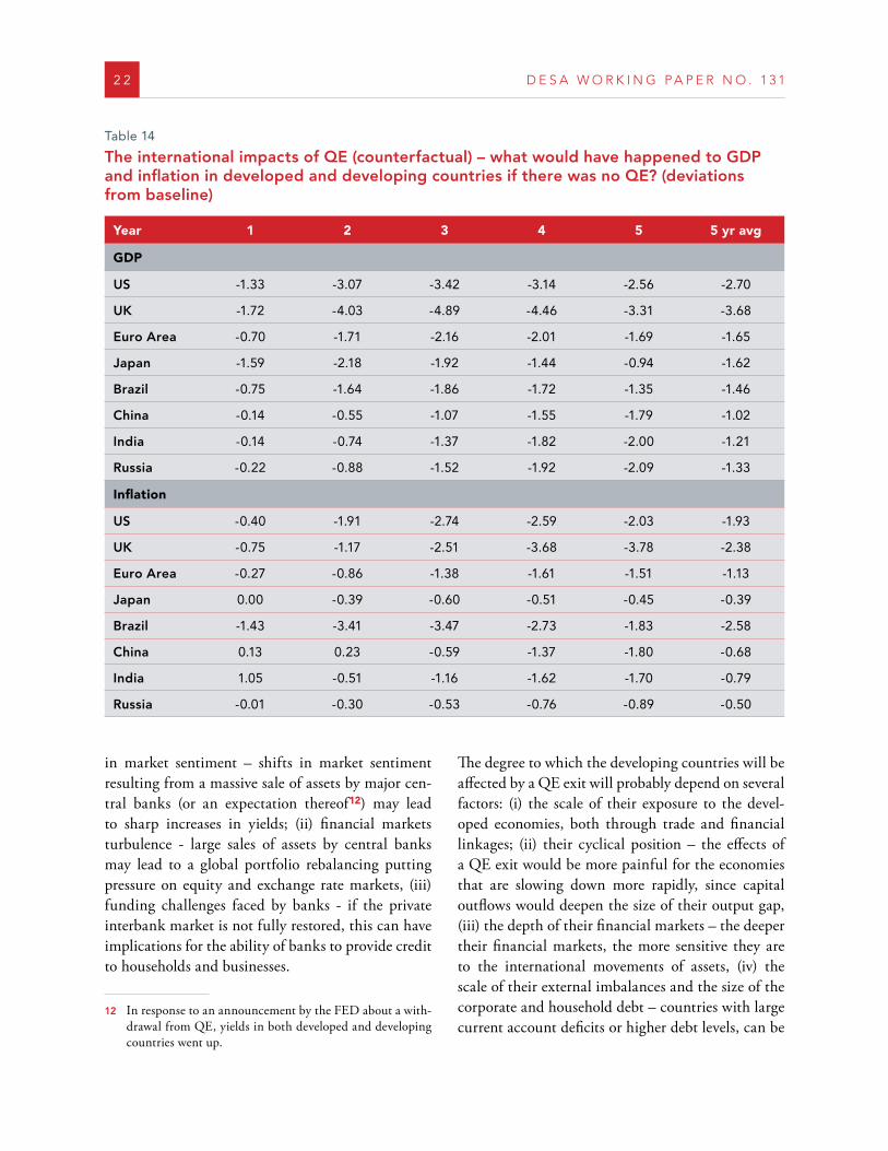
First, we look at the impact of higher long term yields in the US, UK, Euro Area, Japan, Brazil, China, In-dia and Russia. Next, we look at the impact of all shocks - shocks to long term yields, as well as shocks to equity prices, and investment premia.

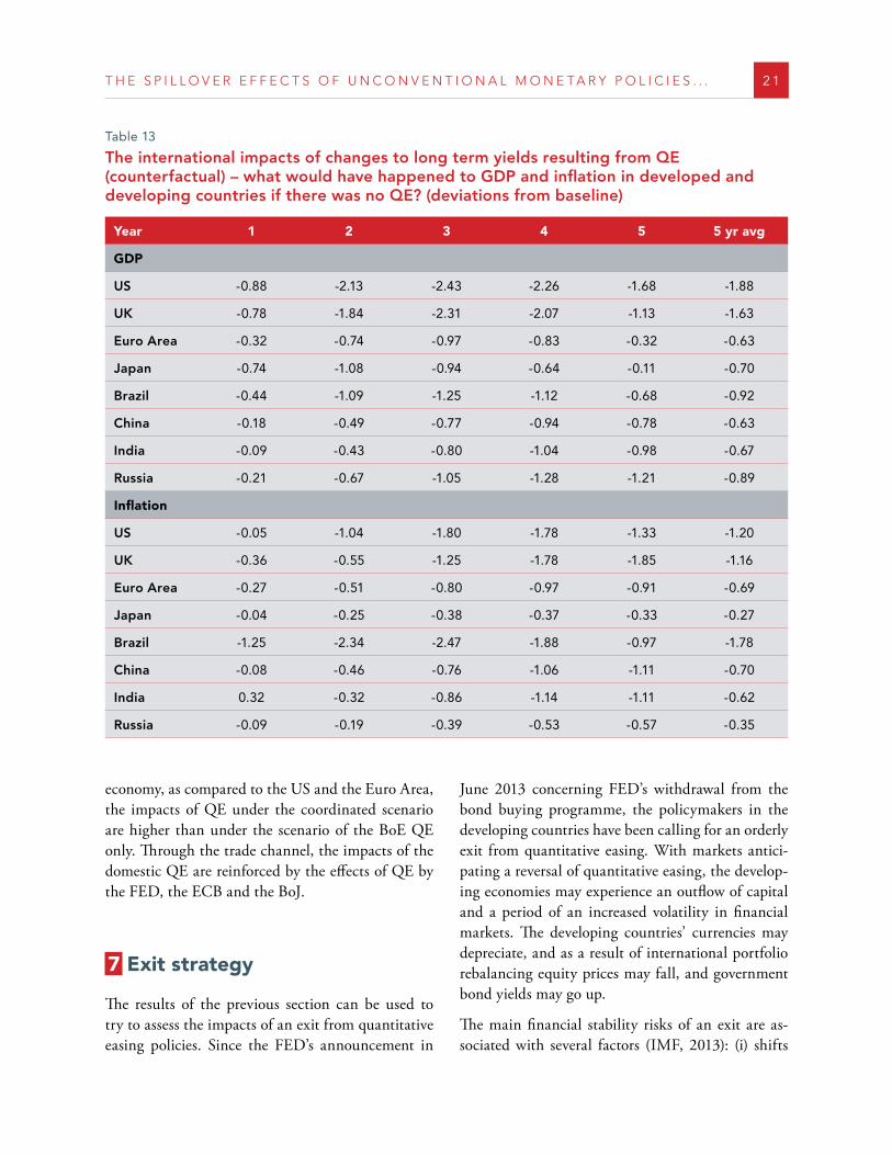
Figure 8 shows the QE effects for individual coun-tries decomposed into those coming from shocks to long term yields and those coming from shocks to equity prices and investment premia. Detailed re-sults are shown in tables 13 and 14. Up to about 70 per cent of the impact can be attributed to changes in term premium. In the case of the UK, the equity market impact of QE seems to be slightly stronger.

In terms of the real impacts, the developed countries that react strongest to global changes to long term yields are the US and the UK, and among the de-veloping countries Brazil is the most sensitive one. The response of the Euro Area, Chinese and Indian economies is more muted. The Brazilian and the UK cases are particularly interesting. Brazil is least impacted under the uncoordinated scenario, while it is much more affected under the coordinated sce-nario. This results from the fact that trade spillovers in the case of Brazil are relatively small as compared to the other developing countries. Spillovers through the financial markets (and especially those affecting long term yields) are, however, biggest in Brazil. In the case of the UK, which is a relatively small

Figure 8

Term premium and equity and investment premia effects – GDP and inflation changes

GDP impact

-4.00

-3.00

-0.50

-3.50

-2.50

0.00

-1.50

-2.00

-1.00

Inflation impact

-3.00

-2.50

-1.00

0.00

-2.00

-1.50

0.50

-0.50

US UK EuroArea

Japan

Equity and investment premia effects Term premium effects

Brazil China India Russia US UK EuroArea

Japan Brazil China India Russia

T H E S P I L L O V E R E F F E C T S O F U N C O N V E N T I O N A L M O N E T A R Y P O L I C I E S . . . 2 1

economy, as compared to the US and the Euro Area, the impacts of QE under the coordinated scenario are higher than under the scenario of the BoE QE only. Through the trade channel, the impacts of the domestic QE are reinforced by the effects of QE by the FED, the ECB and the BoJ.

7 Exit strategy

The results of the previous section can be used to try to assess the impacts of an exit from quantitative easing policies. Since the FED’s announcement in

June 2013 concerning FED’s withdrawal from the bond buying programme, the policymakers in the developing countries have been calling for an orderly exit from quantitative easing. With markets antici-pating a reversal of quantitative easing, the develop-ing economies may experience an outflow of capital and a period of an increased volatility in financial markets. The developing countries’ currencies may depreciate, and as a result of international portfolio rebalancing equity prices may fall, and government bond yields may go up.

The main financial stability risks of an exit are as-sociated with several factors (IMF, 2013): (i) shifts

Table 13

The international impacts of changes to long term yields resulting from QE (counterfactual) – what would have happened to GDP and inflation in developed and developing countries if there was no QE? (deviations from baseline)

Year 1 2 3 4 5 5 yr avg

GDP

US -0 .88 -2 .13 -2 .43 -2 .26 -1 .68 -1 .88

UK -0 .78 -1 .84 -2 .31 -2 .07 -1 .13 -1 .63

Euro Area -0 .32 -0 .74 -0 .97 -0 .83 -0 .32 -0 .63

Japan -0 .74 -1 .08 -0 .94 -0 .64 -0 .11 -0 .70

Brazil -0 .44 -1 .09 -1 .25 -1 .12 -0 .68 -0 .92

China -0 .18 -0 .49 -0 .77 -0 .94 -0 .78 -0 .63

India -0 .09 -0 .43 -0 .80 -1 .04 -0 .98 -0 .67

Russia -0 .21 -0 .67 -1 .05 -1 .28 -1 .21 -0 .89

Inflation

US -0 .05 -1 .04 -1 .80 -1 .78 -1 .33 -1 .20

UK -0 .36 -0 .55 -1 .25 -1 .78 -1 .85 -1 .16

Euro Area -0 .27 -0 .51 -0 .80 -0 .97 -0 .91 -0 .69

Japan -0 .04 -0 .25 -0 .38 -0 .37 -0 .33 -0 .27

Brazil -1 .25 -2 .34 -2 .47 -1 .88 -0 .97 -1 .78

China -0 .08 -0 .46 -0 .76 -1 .06 -1 .11 -0 .70

India 0 .32 -0 .32 -0 .86 -1 .14 -1 .11 -0 .62

Russia -0 .09 -0 .19 -0 .39 -0 .53 -0 .57 -0 .35

2 2 D E S A W O R K I N G P A P E R N O . 1 3 1

in market sentiment – shifts in market sentiment resulting from a massive sale of assets by major cen-tral banks (or an expectation thereof12) may lead to sharp increases in yields; (ii) financial markets turbulence - large sales of assets by central banks may lead to a global portfolio rebalancing putting pressure on equity and exchange rate markets, (iii) funding challenges faced by banks - if the private interbank market is not fully restored, this can have implications for the ability of banks to provide credit to households and businesses.

12 In response to an announcement by the FED about a with-drawal from QE, yields in both developed and developing countries went up.

The degree to which the developing countries will be affected by a QE exit will probably depend on several factors: (i) the scale of their exposure to the devel-oped economies, both through trade and financial linkages; (ii) their cyclical position – the effects of a QE exit would be more painful for the economies that are slowing down more rapidly, since capital outflows would deepen the size of their output gap, (iii) the depth of their financial markets – the deeper their financial markets, the more sensitive they are to the international movements of assets, (iv) the scale of their external imbalances and the size of the corporate and household debt – countries with large current account deficits or higher debt levels, can be

Table 14

The international impacts of QE (counterfactual) – what would have happened to GDP and inflation in developed and developing countries if there was no QE? (deviations from baseline)

Year 1 2 3 4 5 5 yr avg

GDP

US -1 .33 -3 .07 -3 .42 -3 .14 -2 .56 -2 .70

UK -1 .72 -4 .03 -4 .89 -4 .46 -3 .31 -3 .68

Euro Area -0 .70 -1 .71 -2 .16 -2 .01 -1 .69 -1 .65

Japan -1 .59 -2 .18 -1 .92 -1 .44 -0 .94 -1 .62

Brazil -0 .75 -1 .64 -1 .86 -1 .72 -1 .35 -1 .46

China -0 .14 -0 .55 -1 .07 -1 .55 -1 .79 -1 .02

India -0 .14 -0 .74 -1 .37 -1 .82 -2 .00 -1 .21

Russia -0 .22 -0 .88 -1 .52 -1 .92 -2 .09 -1 .33

Inflation

US -0 .40 -1 .91 -2 .74 -2 .59 -2 .03 -1 .93

UK -0 .75 -1 .17 -2 .51 -3 .68 -3 .78 -2 .38

Euro Area -0 .27 -0 .86 -1 .38 -1 .61 -1 .51 -1 .13

Japan 0 .00 -0 .39 -0 .60 -0 .51 -0 .45 -0 .39

Brazil -1 .43 -3 .41 -3 .47 -2 .73 -1 .83 -2 .58

China 0 .13 0 .23 -0 .59 -1 .37 -1 .80 -0 .68

India 1 .05 -0 .51 -1 .16 -1 .62 -1 .70 -0 .79

Russia -0 .01 -0 .30 -0 .53 -0 .76 -0 .89 -0 .50

T H E S P I L L O V E R E F F E C T S O F U N C O N V E N T I O N A L M O N E T A R Y P O L I C I E S . . . 2 3

more vulnerable, (v) policy actions in the developing countries aimed at mitigating the effects of excessive capital outflows.

It should be mentioned that the short term capital flows have weakened recently, and equity valuations in the developing countries seem to be relatively low. This may imply that the risks of an exit are largely in bond markets13.

The macroeconomic impacts of a QE exit can be relatively limited, however, this is conditional on the behaviour of investors in bond markets, and policy actions aimed at mitigating instabilities in the finan-cial markets.

REFERENCES

Bank of England, 2012, The Distributional Effects of As-set Purchases, BoE Quarterly Bulletin (Q3): 254–66

Bauer, MD., Neely C., 2013, International Channels of the Fed’s Unconventional Monetary Policy, Working Paper Series 2012-028B, Federal Reserve Bank of St. Louis.

Baumeister C., Benati L, 2010, Unconventional Mone-tary Policy and the Great Recession: Estimating the Impact of a Compression in the Yield Spread at the Zero Lower Bound, ECB WP 1258

Bean C., 2012, Panel remarks: global aspects of uncon-ventional monetary policies, Conference on quan-titative easing and other unconventional monetary policies, Bank of England

Benford, J., Berry, S., Nikolov, K. and C. Young, 2009, Quantitative Easing, Quarterly Bulletin, Bank of England, Q2

Borio, C and Disyatat, P, 2009, Unconventional mone-tary policies: an appraisal, BIS Working Paper No.292

Chen, H, Cúrdia, V and Ferrero, A, 2011, The macroeco-nomic effects of large-scale asset purchase programs, FED NY Staff Report No. 527.

Chinn M., 2013, Global spillovers and domestic mone-tary policy: the impacts on exchange rates and other asset prices, Paper prepared for the 12th BIS annual conference “Navigating the great recession: what role for monetary policy?” 20-21 June 2013, Luzerne, Switzerland

13 I thank Ingo Pitterle for this idea.

Collignon S. et al., 2012, Unconventional monetary policy measures: a comparison of the ECB, FED and BoE, Directorate General for Internal Policies, Euro-pean Parliament

D’Amico, S., W. English, D. Lopez-Salido and E. Nel-son, 2012, The Federal Reserve’s Large-Scale Asset Purchase Programmes: Rationale and Effects, The Economic Journal 122 (564)

European Central Bank, 2012, Impact of the Two Three-Year Longer-Term Refinancing Operations, ECB Monthly Bulletin (March)

Fawley B., Neely Ch., 2013, Four stories of quantitative easing, Federal Reserve Bank of St. Luis Review, Jan-uary/February 2013, 95(1)

Fratzscher M., Lo Duca M., Straub R., 2013, On the International Spillovers of U.S. Quantitative Easing, ECB WP 1557

Gagnon, J., Raskin, M., Remasche, Sack B, 2011, The Financial Market Effects of the Federal Reserve’s Large-Scale Asset Purchases, International Journal of Central Banking 7(1)

Gambacorta L., Hofmann B., Peersman G., 2012, The effectiveness of unconventional monetary policy at the zero lower bound: a cross country analysis, BIS WP 384

García-Cicco J., 2011, On the Quantitative Effects of Unconventional Monetary Policies, International Journal of Central Banking 7(1).

Hamilton J., Wu J., 2011, Policy Tools in a Zero Lower Bound Environment, NBER WP 16956.

Hancock D, Passmore W, 2011, Did the Federal Re-serve’s MBS purchase program lower mortgage rates?, Finance and Economics Discussion Series 2011-01, Board of Governors of the Federal Reserve System.

Hiroshi U., 2010, Effects of the Quantitative Easing Pol-icy: A survey of Empirical Analyses, Working Paper Series, No 06-E-10, Bank of Japan.

IMF, 2013, Global impact and challenges of unconven-tional monetary policy, IMF Policy Paper, October 2013

IMF, 2013, IMF multilateral policy issues report: spillo-ver report, August 2013-11-07

IMF, 2013, Unconventional monetary policies – recent experience and prospects, IMF, April 2013

Joyce M., 2012, Quantitative easing and other unconven-tional monetary policies: BoE conference summary, BoE Quarterly Bulletin

Joyce, M, Tong, M and Woods, R, 2011, The United King-dom’s quantitative easing policy: design, operation and impact, BoE Quarterly Bulletin, Vol. 51, No. 3

2 4 D E S A W O R K I N G P A P E R N O . 1 3 1

Joyce, M., Lasaosa A, Stevens I, Tong M, 2010, The Fi-nancial Market Impact of uantitative Easing, Work-ing Paper 393, Bank of England.

Kapetanios G., Mumtaz H, Stevens I, Theodoridis K, 2012, Assessing the Economy-wide Effects of Quan-titative Easing, BoE WP 443.

Kimura T., Small D., 2004, Quantitative monetary eas-ing and risk in financial asset markets, Finance and Economics Discussion Series, Division of Research and Statistics and Monetary Affairs, Federal Reserve Board, Washington D.C.

Krishnamurthy A, Vissing-Jorgensen A, 2011, The Effects of Quantitative Easing on Interest Rates, Kellogg School of Management, Northwestern University.

Neely, C. J., 2012, The Large-Scale Asset Purchases Had Large International Effects, Federal Reserve Bank of St. Louis Working Paper No. 2010-018D

Santor E., Suchanek L., 2013, Unconventional Monetary Policies: evolving practices, their effects and potential costs, Bank of Canada Review

Ueda K, 2012, The Effectiveness of Non-traditional Monetary Policy Measures: the Case of the Bank of Japan, The Japanese Economic Review, Vol. 63(1).

Williams, J C, 2011, Unconventional monetary policy: lessons from the past three years, FRBSF Economic Letter No. 2011-31, 3 October

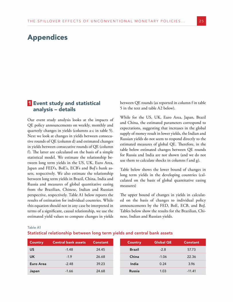
T H E S P I L L O V E R E F F E C T S O F U N C O N V E N T I O N A L M O N E T A R Y P O L I C I E S . . . 2 5

Appendices

Table A1

Statistical relationship between long term yields and central bank assets

Country Central bank assets Constant Country Global QE Constant

US -1 .48 24 .45 Brazil -2 .8 57 .73

UK -1 .9 26 .68 China -1 .06 22 .36

Euro Area -2 .48 39 .23 India 0 .24 3 .96

Japan -1 .66 24 .68 Russia 1 .03 -11 .41

1 Event study and statisticalanalysis – details

Our event study analysis looks at the impacts of QE policy announcements on weekly, monthly and quarterly changes in yields (columns a-c in table 5). Next we look at changes in yields between consecu-tive rounds of QE (column d) and estimated changes in yields between consecutive rounds of QE (column f). The latter are calculated on the basis of a simple statistical model. We estimate the relationship be-tween long term yields in the US, UK, Euro Area, Japan and FED’s, BoE’s, ECB’s and BoJ’s bank as-sets, respectively. We also estimate the relationship between long term yields in Brazil, China, India and Russia and measures of global quantitative easing from the Brazilian, Chinese, Indian and Russian perspective, respectively. Table A1 below reports the results of estimation for individual countries. While this equation should not in any case be interpreted in terms of a significant, causal relationship, we use the estimated yield values to compute changes in yields

between QE rounds (as reported in column f in table 5 in the text and table A2 below).

While for the US, UK, Euro Area, Japan, Brazil and China, the estimated parameters correspond to expectations, suggesting that increases in the global supply of money result in lower yields, the Indian and Russian yields do not seem to respond directly to the estimated measures of global QE. Therefore, in the table below estimated changes between QE rounds for Russia and India are not shown (and we do not use them to calculate shocks in columns f and g).

Table below shows the lower bound of changes in long term yields in the developing countries (cal-culated on the basis of global quantitative easing measures)

The upper bound of changes in yields in calculat-ed on the basis of changes to individual policy announcements by the FED, BoE, ECB, and BoJ. Tables below show the results for the Brazilian, Chi-nese, Indian and Russian yields.

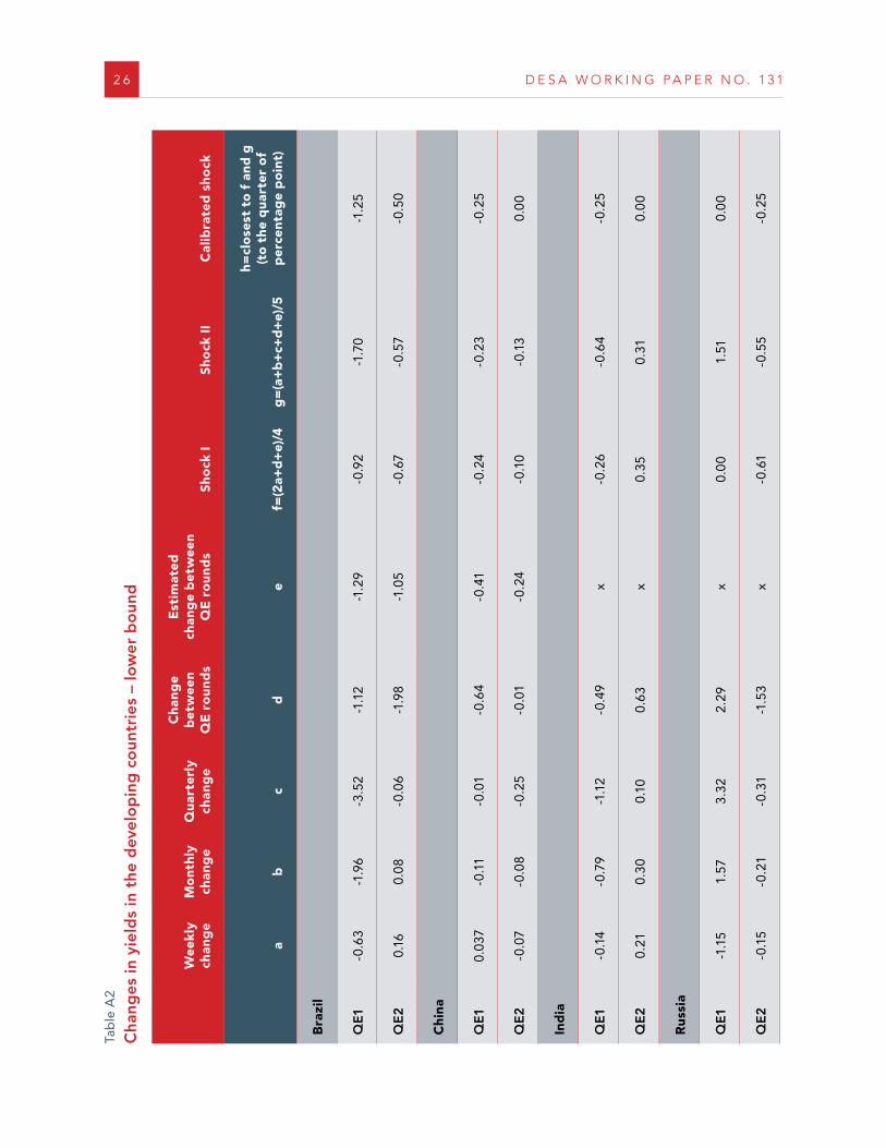
2 6 D E S A W O R K I N G P A P E R N O . 1 3 1

Tab

le A

2

Cha

nges

in y

ield

s in

the

dev

elo

pin

g c

oun

trie

s –

low

er b

oun

d

 W

eekl

y ch

ang

eM

ont

hly

chan

ge

Qua

rter

ly

chan

ge

Cha

nge

bet

wee

n Q

E r

oun

ds

Est

imat

ed

chan

ge

bet

wee

n Q

E r

oun

ds

Sho

ck I

Sho

ck I

IC

alib

rate

d s

hock

 a

bc

de

f=(2

a+d

+e)

/4g

=(a

+b

+c+

d+

e)/5

h=cl

ose

st t

o f

and

g

(to

the

qua

rter

of

per

cent

age

po

int)

Bra

zil

  

  

  

  

QE1

-0 .6

3-1

.96

-3 .5

2-1

.12

-1 .2

9-0

.92

-1 .7

0-1

.25

QE

20 .

160 .

08-0

.06

-1 .9

8-1

.05

-0 .6

7-0

.57

-0 .5

0

Chi

na 

  

  

  

 

QE1

0 .03

7-0

.11

-0 .0

1-0

.64

-0 .4

1-0

.24

-0 .2

3-0

.25

QE

2-0

.07

-0 .0

8-0

.25

-0 .0

1-0

.24

-0 .1

0-0

.13

0 .0

0

Ind

ia 

  

  

  

 

QE1

-0 .1

4-0

.79

-1 .1

2-0

.49

x-0

.26

-0 .6

4-0

.25

QE

20 .

210 .

300 .

100 .

63x

0 .35

0 .31

0 .0

0

Rus

sia

  

  

  

QE1

-1 .1

51 .

573 .

322 .

29x

0 .0

01 .

510 .

00

QE

2-0

.15

-0 .2

1-0

.31

-1 .5

3x

-0 .6

1-0

.55

-0 .2

5

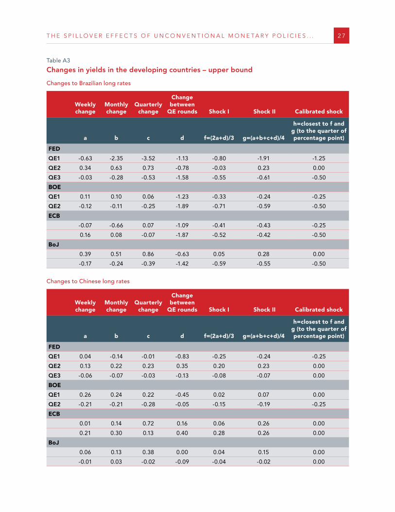
T H E S P I L L O V E R E F F E C T S O F U N C O N V E N T I O N A L M O N E T A R Y P O L I C I E S . . . 2 7

Table A3

Changes in yields in the developing countries – upper bound

Changes to Brazilian long rates

 Weekly change

Monthly change

Quarterly change

Change between

QE rounds Shock I Shock II Calibrated shock

  a b c d f=(2a+d)/3 g=(a+b+c+d)/4

h=closest to f and g (to the quarter of percentage point)

FED              

QE1 -0 .63 -2 .35 -3 .52 -1 .13 -0 .80 -1 .91 -1 .25

QE2 0 .34 0 .63 0 .73 -0 .78 -0 .03 0 .23 0 .00

QE3 -0 .03 -0 .28 -0 .53 -1 .58 -0 .55 -0 .61 -0 .50

BOE              

QE1 0 .11 0 .10 0 .06 -1 .23 -0 .33 -0 .24 -0 .25

QE2 -0 .12 -0 .11 -0 .25 -1 .89 -0 .71 -0 .59 -0 .50

ECB              

  -0 .07 -0 .66 0 .07 -1 .09 -0 .41 -0 .43 -0 .25

  0 .16 0 .08 -0 .07 -1 .87 -0 .52 -0 .42 -0 .50

BoJ      

  0 .39 0 .51 0 .86 -0 .63 0 .05 0 .28 0 .00

  -0 .17 -0 .24 -0 .39 -1 .42 -0 .59 -0 .55 -0 .50

Changes to Chinese long rates

 Weekly change

Monthly change

Quarterly change

Change between

QE rounds Shock I Shock II Calibrated shock

  a b c d f=(2a+d)/3 g=(a+b+c+d)/4

h=closest to f and g (to the quarter of percentage point)

FED              

QE1 0 .04 -0 .14 -0 .01 -0 .83 -0 .25 -0 .24 -0 .25

QE2 0 .13 0 .22 0 .23 0 .35 0 .20 0 .23 0 .00

QE3 -0 .06 -0 .07 -0 .03 -0 .13 -0 .08 -0 .07 0 .00

BOE              

QE1 0 .26 0 .24 0 .22 -0 .45 0 .02 0 .07 0 .00

QE2 -0 .21 -0 .21 -0 .28 -0 .05 -0 .15 -0 .19 -0 .25

ECB              

  0 .01 0 .14 0 .72 0 .16 0 .06 0 .26 0 .00

  0 .21 0 .30 0 .13 0 .40 0 .28 0 .26 0 .00

BoJ              

  0 .06 0 .13 0 .38 0 .00 0 .04 0 .15 0 .00

  -0 .01 0 .03 -0 .02 -0 .09 -0 .04 -0 .02 0 .00

2 8 D E S A W O R K I N G P A P E R N O . 1 3 1

Table A3

Changes in yields in the developing countries – upper bound (continue)

Changes to Indian long rates

 Weekly change

Monthly change

Quarterly change

Change between

QE rounds Shock I Shock II Calibrated shock

  a b c d f=(2a+d)/3 g=(a+b+c+d)/4

h=closest to f and g (to the quarter of percentage point)

FED              

QE1 -0 .14 -0 .96 -1 .12 -0 .80 -0 .36 -0 .75 -0 .50

QE2 -0 .10 -0 .04 -0 .02 1 .06 0 .29 0 .23 0 .00

QE3 -0 .03 -0 .03 -0 .02 -0 .38 -0 .15 -0 .11 0 .00

BOE            

QE1 0 .71 0 .80 0 .74 -0 .12 0 .43 0 .53 0 .00

QE2 -0 .06 0 .00 0 .02 0 .52 0 .13 0 .12 0 .00

ECB              

  0 .01 0 .14 0 .72 0 .16 0 .06 0 .26 0 .00

  0 .21 0 .30 0 .13 0 .40 0 .28 0 .26 0 .00

BoJ          

  -0 .02 -0 .01 0 .02 0 .51 0 .16 0 .13 0 .00

  -0 .11 0 .16 0 .35 0 .14 -0 .03 0 .13 0 .00

Changes in Russian long rates

 Weekly change

Monthly change

Quarterly change

Change between

QE rounds Shock I Shock II Calibrated shock

  a b c d f=(2a+d)/3 g=(a+b+c+d)/4

h=closest to f and g (to the quarter of percentage point)

FED              

QE1 -1 .15 1 .51 3 .32 2 .88 0 .19 0 .87 0 .00

QE2 -0 .11 0 .16 0 .17 -1 .69 -0 .64 -0 .90 -0 .25

QE3 0 .03 -0 .15 -0 .51 -1 .01 -0 .32 -0 .49 -0 .25

BOE              

QE1 -0 .47 -0 .47 -0 .82 1 .42 0 .16 0 .48 0 .00

QE2 -0 .55 -0 .60 -0 .62 -1 .32 -0 .81 -0 .94 -0 .25

ECB            

  -0 .48 -0 .47 -0 .87 0 .08 -0 .29 -0 .20 -0 .25

  -0 .15 -0 .21 -0 .30 -0 .83 -0 .38 -0 .49 -0 .25

BoJ              

  -0 .03 0 .04 0 .13 -1 .02 -0 .36 -0 .52 -0 .25

  0 .07 0 .06 0 .34 0 .09 0 .08 0 .08 0 .00

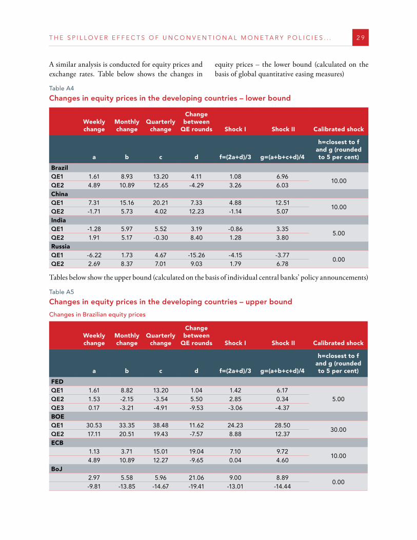
T H E S P I L L O V E R E F F E C T S O F U N C O N V E N T I O N A L M O N E T A R Y P O L I C I E S . . . 2 9

Table A4

Changes in equity prices in the developing countries – lower bound

 Weekly change

Monthly change

Quarterly change

Change between

QE rounds Shock I Shock II Calibrated shock

  a b c d f=(2a+d)/3 g=(a+b+c+d)/4

h=closest to f and g (rounded to 5 per cent)

Brazil              QE1 1 .61 8 .93 13 .20 4 .11 1 .08 6 .96

10 .00QE2 4 .89 10 .89 12 .65 -4 .29 3 .26 6 .03China          QE1 7 .31 15 .16 20 .21 7 .33 4 .88 12 .51

10 .00QE2 -1 .71 5 .73 4 .02 12 .23 -1 .14 5 .07India              QE1 -1 .28 5 .97 5 .52 3 .19 -0 .86 3 .35

5 .00QE2 1 .91 5 .17 -0 .30 8 .40 1 .28 3 .80Russia          QE1 -6 .22 1 .73 4 .67 -15 .26 -4 .15 -3 .77

0 .00QE2 2 .69 8 .37 7 .01 9 .03 1 .79 6 .78

Tables below show the upper bound (calculated on the basis of individual central banks’ policy announcements)

Table A5

Changes in equity prices in the developing countries – upper bound

Changes in Brazilian equity prices

 Weekly change

Monthly change

Quarterly change

Change between

QE rounds Shock I Shock II Calibrated shock

  a b c d f=(2a+d)/3 g=(a+b+c+d)/4

h=closest to f and g (rounded to 5 per cent)

FED              QE1 1 .61 8 .82 13 .20 1 .04 1 .42 6 .17

5 .00QE2 1 .53 -2 .15 -3 .54 5 .50 2 .85 0 .34QE3 0 .17 -3 .21 -4 .91 -9 .53 -3 .06 -4 .37BOE          QE1 30 .53 33 .35 38 .48 11 .62 24 .23 28 .50

30 .00QE2 17 .11 20 .51 19 .43 -7 .57 8 .88 12 .37ECB              1 .13 3 .71 15 .01 19 .04 7 .10 9 .72

10 .00  4 .89 10 .89 12 .27 -9 .65 0 .04 4 .60BoJ                2 .97 5 .58 5 .96 21 .06 9 .00 8 .89

0 .00  -9 .81 -13 .85 -14 .67 -19 .41 -13 .01 -14 .44

A similar analysis is conducted for equity prices and exchange rates. Table below shows the changes in

equity prices – the lower bound (calculated on the basis of global quantitative easing measures)

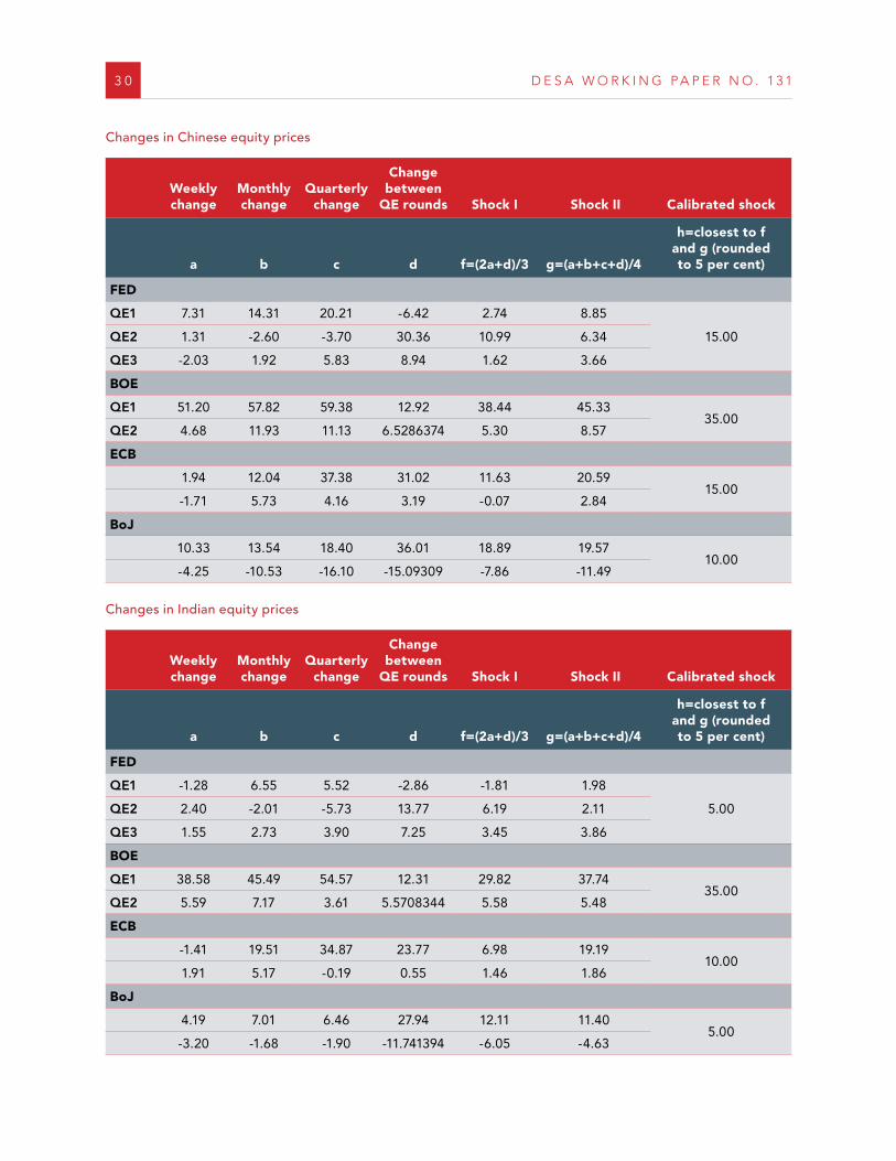
3 0 D E S A W O R K I N G P A P E R N O . 1 3 1

Changes in Chinese equity prices

 Weekly change

Monthly change

Quarterly change

Change between

QE rounds Shock I Shock II Calibrated shock

  a b c d f=(2a+d)/3 g=(a+b+c+d)/4

h=closest to f and g (rounded to 5 per cent)

FED              

QE1 7 .31 14 .31 20 .21 -6 .42 2 .74 8 .85

15 .00QE2 1 .31 -2 .60 -3 .70 30 .36 10 .99 6 .34

QE3 -2 .03 1 .92 5 .83 8 .94 1 .62 3 .66

BOE              

QE1 51 .20 57 .82 59 .38 12 .92 38 .44 45 .3335 .00

QE2 4 .68 11 .93 11 .13 6 .5286374 5 .30 8 .57

ECB            

  1 .94 12 .04 37 .38 31 .02 11 .63 20 .5915 .00

  -1 .71 5 .73 4 .16 3 .19 -0 .07 2 .84

BoJ              

  10 .33 13 .54 18 .40 36 .01 18 .89 19 .5710 .00

  -4 .25 -10 .53 -16 .10 -15 .09309 -7 .86 -11 .49

Changes in Indian equity prices

 Weekly change

Monthly change

Quarterly change

Change between

QE rounds Shock I Shock II Calibrated shock

  a b c d f=(2a+d)/3 g=(a+b+c+d)/4

h=closest to f and g (rounded to 5 per cent)

FED              

QE1 -1 .28 6 .55 5 .52 -2 .86 -1 .81 1 .98

5 .00QE2 2 .40 -2 .01 -5 .73 13 .77 6 .19 2 .11

QE3 1 .55 2 .73 3 .90 7 .25 3 .45 3 .86

BOE            

QE1 38 .58 45 .49 54 .57 12 .31 29 .82 37 .7435 .00

QE2 5 .59 7 .17 3 .61 5 .5708344 5 .58 5 .48

ECB            

  -1 .41 19 .51 34 .87 23 .77 6 .98 19 .1910 .00

  1 .91 5 .17 -0 .19 0 .55 1 .46 1 .86

BoJ              

  4 .19 7 .01 6 .46 27 .94 12 .11 11 .405 .00

  -3 .20 -1 .68 -1 .90 -11 .741394 -6 .05 -4 .63

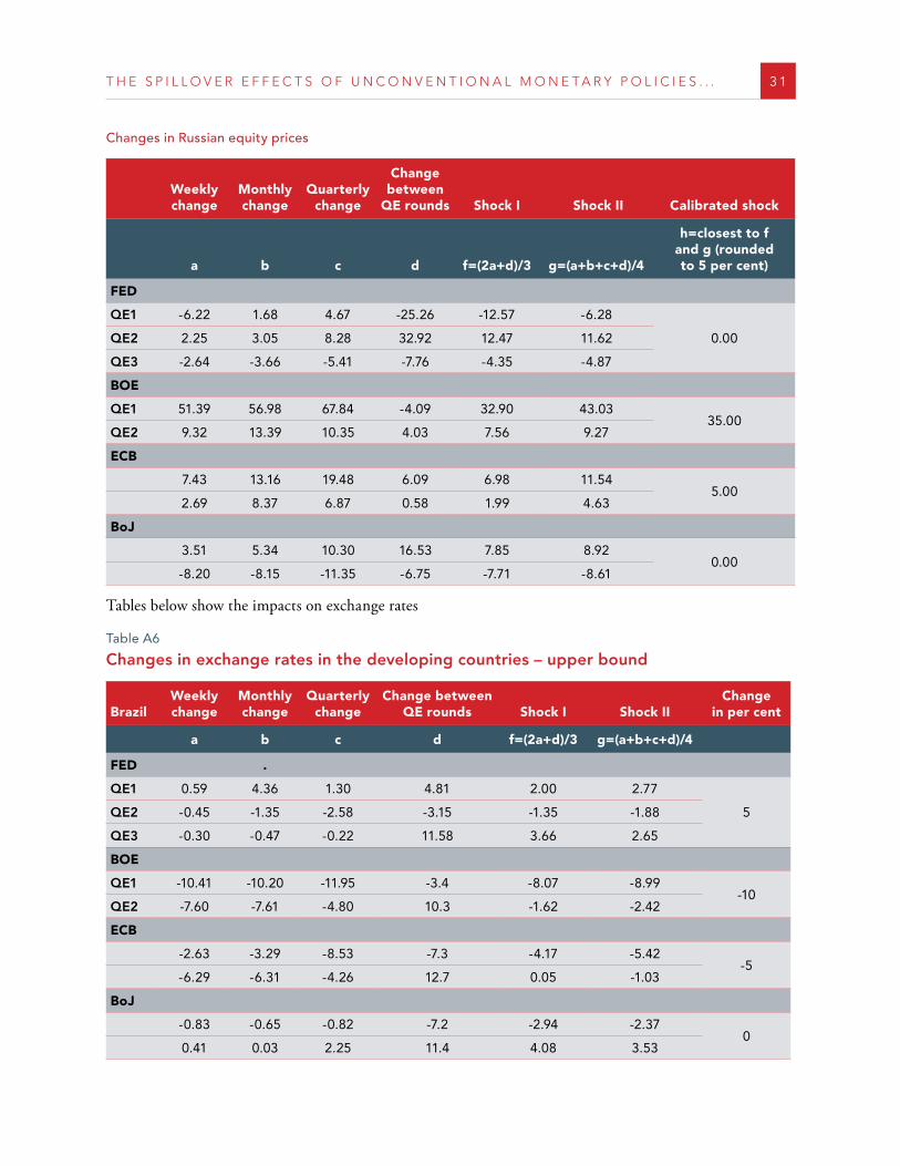
T H E S P I L L O V E R E F F E C T S O F U N C O N V E N T I O N A L M O N E T A R Y P O L I C I E S . . . 3 1

Changes in Russian equity prices

 Weekly change

Monthly change

Quarterly change

Change between

QE rounds Shock I Shock II Calibrated shock

  a b c d f=(2a+d)/3 g=(a+b+c+d)/4

h=closest to f and g (rounded to 5 per cent)

FED              

QE1 -6 .22 1 .68 4 .67 -25 .26 -12 .57 -6 .28

0 .00QE2 2 .25 3 .05 8 .28 32 .92 12 .47 11 .62

QE3 -2 .64 -3 .66 -5 .41 -7 .76 -4 .35 -4 .87

BOE            

QE1 51 .39 56 .98 67 .84 -4 .09 32 .90 43 .0335 .00

QE2 9 .32 13 .39 10 .35 4 .03 7 .56 9 .27

ECB            

  7 .43 13 .16 19 .48 6 .09 6 .98 11 .545 .00

  2 .69 8 .37 6 .87 0 .58 1 .99 4 .63

BoJ              

  3 .51 5 .34 10 .30 16 .53 7 .85 8 .920 .00

  -8 .20 -8 .15 -11 .35 -6 .75 -7 .71 -8 .61

Tables below show the impacts on exchange rates

Table A6

Changes in exchange rates in the developing countries – upper bound

BrazilWeekly change

Monthly change

Quarterly change

Change between QE rounds Shock I Shock II

Change in per cent

  a b c d f=(2a+d)/3 g=(a+b+c+d)/4  

FED   .          

QE1 0 .59 4 .36 1 .30 4 .81 2 .00 2 .77

5QE2 -0 .45 -1 .35 -2 .58 -3 .15 -1 .35 -1 .88

QE3 -0 .30 -0 .47 -0 .22 11 .58 3 .66 2 .65

BOE              

QE1 -10 .41 -10 .20 -11 .95 -3 .4 -8 .07 -8 .99-10

QE2 -7 .60 -7 .61 -4 .80 10 .3 -1 .62 -2 .42

ECB            

  -2 .63 -3 .29 -8 .53 -7 .3 -4 .17 -5 .42-5

  -6 .29 -6 .31 -4 .26 12 .7 0 .05 -1 .03

BoJ              

  -0 .83 -0 .65 -0 .82 -7 .2 -2 .94 -2 .370

  0 .41 0 .03 2 .25 11 .4 4 .08 3 .53

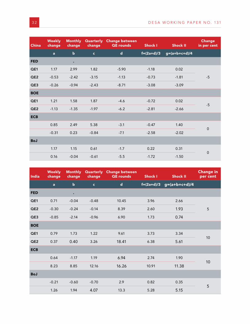
3 2 D E S A W O R K I N G P A P E R N O . 1 3 1

ChinaWeekly change

Monthly change

Quarterly change

Change between QE rounds Shock I Shock II

Change in per cent

  a b c d f=(2a+d)/3 g=(a+b+c+d)/4  

FED   .          

QE1 1 .17 2 .99 1 .82 -5 .90 -1 .18 0 .02

-5QE2 -0 .53 -2 .42 -3 .15 -1 .13 -0 .73 -1 .81

QE3 -0 .26 -0 .94 -2 .43 -8 .71 -3 .08 -3 .09

BOE              

QE1 1 .21 1 .58 1 .87 -4 .6 -0 .72 0 .02-5

QE2 -1 .13 -1 .35 -1 .97 -6 .2 -2 .81 -2 .66

ECB            

  0 .85 2 .49 5 .38 -3 .1 -0 .47 1 .400

  -0 .31 0 .23 -0 .84 -7 .1 -2 .58 -2 .02

BoJ              

  1 .17 1 .15 0 .61 -1 .7 0 .22 0 .310

  0 .16 -0 .04 -0 .61 -5 .5 -1 .72 -1 .50

IndiaWeekly change

Monthly change

Quarterly change

Change between QE rounds Shock I Shock II

Change in per cent

  a b c d f=(2a+d)/3 g=(a+b+c+d)/4  

FED   .          

QE1 0 .71 -0 .04 -0 .48 10 .45 3 .96 2 .66

5QE2 -0 .30 -0 .24 -0 .14 8 .39 2 .60 1 .93

QE3 -0 .85 -2 .14 -0 .96 6 .90 1 .73 0 .74

BOE              

QE1 0 .79 1 .73 1 .22 9 .61 3 .73 3 .3410

QE2 0 .37 0 .40 3 .26 18 .41 6 .38 5 .61

ECB              

  0 .64 -1 .17 1 .19 6 .94 2 .74 1 .9010

  8 .23 8 .85 12 .16 16 .26 10 .91 11 .38

BoJ              

  -0 .21 -0 .60 -0 .70 2 .9 0 .82 0 .355

  1 .26 1 .94 4 .07 13 .3 5 .28 5 .15

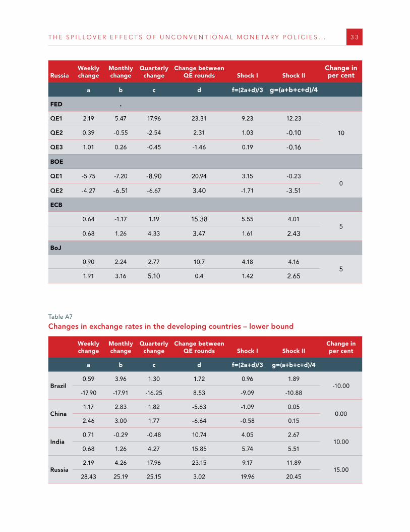
T H E S P I L L O V E R E F F E C T S O F U N C O N V E N T I O N A L M O N E T A R Y P O L I C I E S . . . 3 3

RussiaWeekly change

Monthly change

Quarterly change

Change between QE rounds Shock I Shock II

Change in per cent

  a b c d f=(2a+d)/3 g=(a+b+c+d)/4  

FED   .          

QE1 2 .19 5 .47 17 .96 23 .31 9 .23 12 .23

10QE2 0 .39 -0 .55 -2 .54 2 .31 1 .03 -0 .10

QE3 1 .01 0 .26 -0 .45 -1 .46 0 .19 -0 .16

BOE              

QE1 -5 .75 -7 .20 -8 .90 20 .94 3 .15 -0 .230

QE2 -4 .27 -6 .51 -6 .67 3 .40 -1 .71 -3 .51

ECB              

  0 .64 -1 .17 1 .19 15 .38 5 .55 4 .015

  0 .68 1 .26 4 .33 3 .47 1 .61 2 .43

BoJ              

  0 .90 2 .24 2 .77 10 .7 4 .18 4 .165

  1 .91 3 .16 5 .10 0 .4 1 .42 2 .65

Table A7

Changes in exchange rates in the developing countries – lower bound

 Weekly change

Monthly change

Quarterly change

Change between QE rounds Shock I Shock II

Change in per cent

  a b c d f=(2a+d)/3 g=(a+b+c+d)/4  

Brazil0 .59 3 .96 1 .30 1 .72 0 .96 1 .89

-10 .00-17 .90 -17 .91 -16 .25 8 .53 -9 .09 -10 .88

China1 .17 2 .83 1 .82 -5 .63 -1 .09 0 .05

0 .002 .46 3 .00 1 .77 -6 .64 -0 .58 0 .15

India0 .71 -0 .29 -0 .48 10 .74 4 .05 2 .67

10 .000 .68 1 .26 4 .27 15 .85 5 .74 5 .51

Russia2 .19 4 .26 17 .96 23 .15 9 .17 11 .89

15 .0028 .43 25 .19 25 .15 3 .02 19 .96 20 .45

3 4 D E S A W O R K I N G P A P E R N O . 1 3 1

2 A brief description of NIGEM

For a macroeconometric model to be useful for policy analyses, particular attention must be paid to its long-term equilibrium properties. At the same time, we need to ensure that short-term dynamic properties and underlying estimated properties are consistent with data and well-determined. As far as possible the same long run theoretical structure of NiGEM has been adopted for each of the major industrial countries, except where clear institutional or other factors prevent this. As a result, variations in the properties of each country model reflect genuine differences in data ratios and estimated parameters, rather than different theoretical approaches.

Production and price setting

The major country models rely on an underlying constant-returns-to-scale CES production function with labour-augmenting technical progress.

( )[ ] ρρλργ /1))(1( −−− −+= tLesKsQ (1)

where Q is real output, K is the total capital stock, L is total hours worked and t is an index of labour-aug-menting technical progress. This constitutes the theoretical background for the specifications of the factor demand equations, forms the basis for unit total costs and provides a measure of capacity utilization, which then feed into the price system. The elasticity of substitution is estimated from the labour demand equation, and in general it is around 0.5. Demand for labour and capital are determined by profit maximisation of firms, implying that the long-run labour-output ratio depends on real wage costs and technical progress, while the long-run capital output ratio depends on the real user cost of capital

{ }[ ] )/ln()1()ln()ln()1()1(ln)( pwtQsLLn σλσγσβσ −−−+−−−= (2)

[ ] )/ln()ln()ln()1()ln()( pcQsKLn σγσβσ −+−−= (3)

where w/p is the real wage and c/p is the real user cost of capital. The user cost of capital is influenced by corporate taxes and depreciation and is a weighted average of the cost of equity finance and the margin ad-justed long real rate, with weights that vary with the size of equity markets as compared to the private sector capital stock. Business investment is determined by the error correction based relationship between actual and equilibrium capital stocks. Government investment depends upon trend output and the real interest rate in the long run. Prices are determined as a constant mark-up over marginal costs in the long term.

Labour market

NiGEM assumes employers have a right to manage. Hence the bargain in the labour market is over the real wage. Real wages, therefore, depend on the level of trend labour productivity as well as the rate of unemploy-ment. Labour markets embody rational expectations and wage bargainers use model consistent expectations. The dynamics of wage-setting depend upon the error correction term in the equation, the split between lagged inflation and forward inflation, and the impact of unemployment on the wage bargain. There is no explicit equation for sustainable employment in the model, but as the wage and price system is complete the model delivers equilibrium levels of employment and unemployment. An estimate of the NAIRU can be obtained by substituting the mark-up adjusted unit total cost equation into the wage equation and solving for the unemployment rate. Labour supply is determined by demographics, migration and the participation rate.

T H E S P I L L O V E R E F F E C T S O F U N C O N V E N T I O N A L M O N E T A R Y P O L I C I E S . . . 3 5

Consumption, personal income and wealth

Consumption decisions depend on real disposable income and real wealth in the long run, and follow the pattern discussed in Barrell and Davis (2007). Total wealth is composed of financial and tangible (housing) wealth where the latter data is available.

(ln )ln()1()ln() RTWRFNRPDIC +−++= ββα (4)

where C is real consumption, RPDI is real personal disposable income, RFN is real net financial wealth and RTW is real tangible wealth. The dynamics of adjustment to the long run are largely data based, and differ between countries to take account of differences in the relative importance of types of wealth and of liquidity constraints.

Financial markets

We generally assume that exchange rates are forward looking, and ‘jump’ when there is news. The size of the jump depends on the expected future path of interest rates and risk premia, solving an uncovered interest parity condition, and these, in turn, are determined by policy rules adopted by monetary authorities:

)1)](1/()1)[(1()( rprxrarhtRXtRX ++++= (5)

where RX is the exchange rate, rh is the home interest rate set in line with a policy rule, ra is the interest rate abroad and rprx is the risk premium. We assume that bond and equity markets are forward looking, and long-term interest rates are a forward convolution of expected short-term interest rates. Forward looking equity prices are determined by the discounted present value of expected profits.

Public sector

Each country has a set of equations for the public sector. Direct and indirect taxes depend upon their re-spective tax bases and on the tax rate. Government spending on current goods and services and investment spending depend in part on current plans, and by default rise with trend output. Transfer payments depend upon unemployment and the dependency ratio as well as on policy. Government interest payments are deter-mined by a perpetual inventory model based on the flow deficit and the stock of debt, with the appropriate structure of short and long-term interest payments on the debt stock. Budget deficits are kept within bounds in the longer term (Barrell and Sefton, 1997) through a targeted adjustment on income tax rates.

External trade

International linkages come from patterns of trade, the influence of trade prices on domestic price, the im-pacts of exchange rates and patterns of asset holding and associated income flows. The volumes of exports and imports of goods and services are determined by foreign or domestic demand, respectively, and by competi-tiveness as measured by relative prices or costs. The estimated relationships also include measures to capture globalization, European integration and sector-specific developments. Exporters are assumed to compete against others who export to the same market and domestic producers via relative prices; demand is given by a share of imports in the markets to which the country has previously exported. Imports depend on import prices relative to domestic prices and on domestic total final expenditure. As exports depend on imports, they will rise together in the model. The overall current balance depends upon the trade balance and net property income from abroad, comprising flows of income on gross foreign assets and outgoings on gross foreign liabilities. Gross national product is GDP plus net factor income from foreigners.

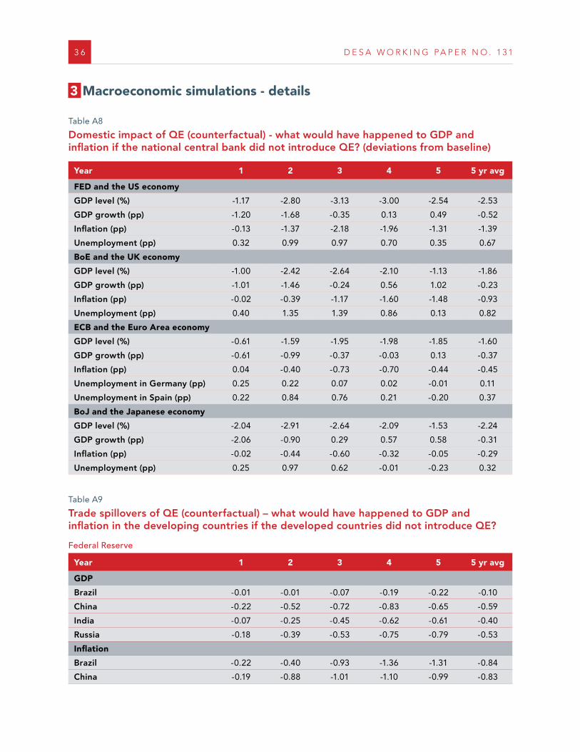
3 6 D E S A W O R K I N G P A P E R N O . 1 3 1

3 Macroeconomic simulations - details

Table A8

Domestic impact of QE (counterfactual) - what would have happened to GDP and inflation if the national central bank did not introduce QE? (deviations from baseline)

Year 1 2 3 4 5 5 yr avg

FED and the US economy  

GDP level (%) -1 .17 -2 .80 -3 .13 -3 .00 -2 .54 -2 .53

GDP growth (pp) -1 .20 -1 .68 -0 .35 0 .13 0 .49 -0 .52

Inflation (pp) -0 .13 -1 .37 -2 .18 -1 .96 -1 .31 -1 .39

Unemployment (pp) 0 .32 0 .99 0 .97 0 .70 0 .35 0 .67

BoE and the UK economy  

GDP level (%) -1 .00 -2 .42 -2 .64 -2 .10 -1 .13 -1 .86

GDP growth (pp) -1 .01 -1 .46 -0 .24 0 .56 1 .02 -0 .23

Inflation (pp) -0 .02 -0 .39 -1 .17 -1 .60 -1 .48 -0 .93

Unemployment (pp) 0 .40 1 .35 1 .39 0 .86 0 .13 0 .82

ECB and the Euro Area economy  

GDP level (%) -0 .61 -1 .59 -1 .95 -1 .98 -1 .85 -1 .60

GDP growth (pp) -0 .61 -0 .99 -0 .37 -0 .03 0 .13 -0 .37

Inflation (pp) 0 .04 -0 .40 -0 .73 -0 .70 -0 .44 -0 .45

Unemployment in Germany (pp) 0 .25 0 .22 0 .07 0 .02 -0 .01 0 .11

Unemployment in Spain (pp) 0 .22 0 .84 0 .76 0 .21 -0 .20 0 .37

BoJ and the Japanese economy  

GDP level (%) -2 .04 -2 .91 -2 .64 -2 .09 -1 .53 -2 .24

GDP growth (pp) -2 .06 -0 .90 0 .29 0 .57 0 .58 -0 .31

Inflation (pp) -0 .02 -0 .44 -0 .60 -0 .32 -0 .05 -0 .29

Unemployment (pp) 0 .25 0 .97 0 .62 -0 .01 -0 .23 0 .32

Table A9

Trade spillovers of QE (counterfactual) – what would have happened to GDP and inflation in the developing countries if the developed countries did not introduce QE?

Federal Reserve

Year 1 2 3 4 5 5 yr avg

GDP  

Brazil -0 .01 -0 .01 -0 .07 -0 .19 -0 .22 -0 .10

China -0 .22 -0 .52 -0 .72 -0 .83 -0 .65 -0 .59

India -0 .07 -0 .25 -0 .45 -0 .62 -0 .61 -0 .40

Russia -0 .18 -0 .39 -0 .53 -0 .75 -0 .79 -0 .53

Inflation  

Brazil -0 .22 -0 .40 -0 .93 -1 .36 -1 .31 -0 .84

China -0 .19 -0 .88 -1 .01 -1 .10 -0 .99 -0 .83

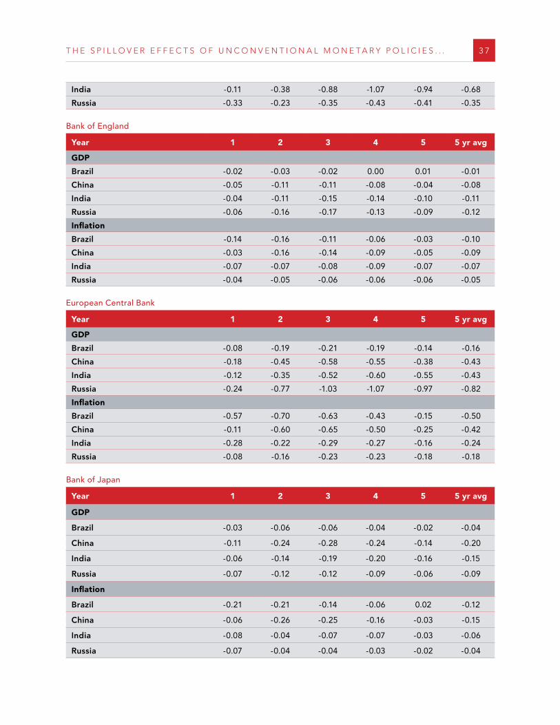
T H E S P I L L O V E R E F F E C T S O F U N C O N V E N T I O N A L M O N E T A R Y P O L I C I E S . . . 3 7

India -0 .11 -0 .38 -0 .88 -1 .07 -0 .94 -0 .68

Russia -0 .33 -0 .23 -0 .35 -0 .43 -0 .41 -0 .35

Bank of England

Year 1 2 3 4 5 5 yr avg

GDP  

Brazil -0 .02 -0 .03 -0 .02 0 .00 0 .01 -0 .01

China -0 .05 -0 .11 -0 .11 -0 .08 -0 .04 -0 .08

India -0 .04 -0 .11 -0 .15 -0 .14 -0 .10 -0 .11

Russia -0 .06 -0 .16 -0 .17 -0 .13 -0 .09 -0 .12

Inflation  

Brazil -0 .14 -0 .16 -0 .11 -0 .06 -0 .03 -0 .10

China -0 .03 -0 .16 -0 .14 -0 .09 -0 .05 -0 .09

India -0 .07 -0 .07 -0 .08 -0 .09 -0 .07 -0 .07

Russia -0 .04 -0 .05 -0 .06 -0 .06 -0 .06 -0 .05

European Central Bank

Year 1 2 3 4 5 5 yr avg

GDP  

Brazil -0 .08 -0 .19 -0 .21 -0 .19 -0 .14 -0 .16

China -0 .18 -0 .45 -0 .58 -0 .55 -0 .38 -0 .43

India -0 .12 -0 .35 -0 .52 -0 .60 -0 .55 -0 .43

Russia -0 .24 -0 .77 -1 .03 -1 .07 -0 .97 -0 .82

Inflation  

Brazil -0 .57 -0 .70 -0 .63 -0 .43 -0 .15 -0 .50

China -0 .11 -0 .60 -0 .65 -0 .50 -0 .25 -0 .42

India -0 .28 -0 .22 -0 .29 -0 .27 -0 .16 -0 .24

Russia -0 .08 -0 .16 -0 .23 -0 .23 -0 .18 -0 .18

Bank of Japan

Year 1 2 3 4 5 5 yr avg

GDP  

Brazil -0 .03 -0 .06 -0 .06 -0 .04 -0 .02 -0 .04

China -0 .11 -0 .24 -0 .28 -0 .24 -0 .14 -0 .20

India -0 .06 -0 .14 -0 .19 -0 .20 -0 .16 -0 .15

Russia -0 .07 -0 .12 -0 .12 -0 .09 -0 .06 -0 .09

Inflation  

Brazil -0 .21 -0 .21 -0 .14 -0 .06 0 .02 -0 .12

China -0 .06 -0 .26 -0 .25 -0 .16 -0 .03 -0 .15

India -0 .08 -0 .04 -0 .07 -0 .07 -0 .03 -0 .06

Russia -0 .07 -0 .04 -0 .04 -0 .03 -0 .02 -0 .04