Is the ECB unconventional monetary policy effective? · 2 Is the ECB unconventional monetary policy effective? An event–study on ECB unconventional monetary policy announcements

GEE Papers

Número 61

setembro de 2016

Is the ECB unconventional monetary policy effective?

Ines Pereira

2

Is the ECB unconventional monetary policy effective?

An event–study on ECB unconventional monetary policy announcements

Ines Pereira

Abstract

After the financial crisis in 2008, many central banks began to use unconventional monetary policy in

order to boost the effective transmission of monetary policy and to provide additional direct monetary

stimulus to the economy. This study will make use of an event study to analyse the impact of those

unconventional monetary policies implemented by the European Central Bank on nominal and real

long-term interest rates. The long-term interest rates being considered are the 10-year government

bond yield, the 5 and 10-year corporate bond yield (AAA and BBB) and the 5y5y swap forward rate

for the Eurozone. The results show that unconventional monetary policy conducted by the ECB had a

significant effect on real and nominal and long-term interest rates. This effect can be more persistent

for a specific group of countries during some announcements, namely the 4th of September of 2014

announcement significantly lowered the 10-year government bond yield and BBB 5-year bond yield

for Portugal and the remaining PIIGS.

JEL Classification: G14, E42, E44

Keywords: Inflation expectations, Unconventional monetary policy, European Central Bank, Long-term interest rates, Event study

3

Contents

1. Introduction ........................................................................................................................................ 5

2. Theoretical Background ................................................................................................................... 10

2.1 The Fisher equation ..................................................................................................................... 10

2.2 Term structure of interest rates ................................................................................................... 11

2.2.1 Expectations Hypothesis .......................................................................................................... 11

2.3 Inflation expectations .................................................................................................................. 12

2.4 Monetary policy in the Eurozone ................................................................................................ 12

2.4.1 Conventional monetary policy in the Eurozone ....................................................................... 13

2.4.2 Unconventional monetary policy in the Eurozone ................................................................... 14

2.4.2.1 Description of the ECB unconventional monetary policy announcements ........................... 15

3. Literature Review.............................................................................................................................. 20

3.1 Previous literature on the effect of unconventional monetary policy in the euro area ................ 20

3.2 Previous literature on the effect of unconventional monetary policy on other central banks:

USA, Japan and England .................................................................................................................. 21

4. Data ................................................................................................................................................... 26

5. Methodology .................................................................................................................................... 27

5.1 Event study .................................................................................................................................. 27

5.2 Statistical significance................................................................................................................ 30

6. Results ............................................................................................................................................... 31

6.1 Overall effect of the ECB unconventional monetary policy ....................................................... 31

6.2 Effect of the ECB unconventional monetary policy per country and per announcement ........... 33

7. Conclusion ........................................................................................................................................ 36

References ............................................................................................................................................. 38

Appendix ............................................................................................................................................... 42

4

List of tables

Table A Longer-term refinancing operations announcements .............................................................. 15

Table B: Target longer-term refinancing operations announcements ................................................... 16

Table C: Securities market programme announcements ....................................................................... 17

Table D: Covered bond purchase programme announcements ............................................................. 18

Table E: Expanded asset purchase programme announcements ........................................................... 18

Table F: Corporate sector purchase programme announcements .......................................................... 19

Table G: Negative deposit facility rate announcements ........................................................................ 19

Table H: Overall significance of the abnormal and cumulative abnormal 10-year government bond

yield changes computed by using the market model. ............................................................................ 32

Table I: Overall significance of the abnormal and cumulative abnormal 10-year government bond

yield changes computed by using the constant mean return model. ..................................................... 32

Table J: Overall significance of the abnormal and cumulative abnormal changes of 5y5y swap forward

rate computed by using the constant mean return model. ..................................................................... 32

Table K: Overall significance of the abnormal and cumulative abnormal changes of AAA 10-year

corporate bond yield computed by using the constant mean return model. .......................................... 33

Table L: Overall significance of the abnormal and cumulative abnormal changes of BBB 10-year


Table M: Overall significance of the abnormal and cumulative abnormal changes of AAA 5-year


Table N: Overall significance of the abnormal and cumulative abnormal changes of BBB 5-year


List of figures

Figure 1 – Key Interest Rates for Eurozone from 1999 to 2016 ........................................................... 13

Figure 2 – Changes in nominal and real long term interest rates around the unconventional monetary

policy announcement on the 4th of September 2014.............................................................................. 35

5

1. Introduction

The global financial crisis of 2008 and the subsequent recession have motivated fundamental changes

in the design and implementation of monetary policy. Many central banks reduced policy rates to near

zero (or even negative) in 2009 and adopted less conventional policies in order to provide additional

monetary stimulus. Central banks of major advanced economies started using unconventional

monetary policies, mainly being purchases of longer-maturity assets. Price stability is a key objective

of any central bank (Gospodinov & Wei, 2015). In order to achieve that, the majority of countries

around the world use the short-term interest rate as the primary monetary policy instrument. By

adjusting the interest rates, central banks can regulate the money supply. If monetary policy-makers

want to decrease the amount of money in an economy, they will increase the interest rate, making it

more attractive to deposit funds at the central bank and reducing borrowing from the central bank.

Instead, if monetary policy-makers want to increase the money supply, they will decrease the interest

rates. Therefore, the interest rate channel plays a very important role in the transmission of monetary

policy.

Nominal interest rates denote payment received by an investor relative to either the asset’s principal

(face) amount or its market price, whereas real interest rates refer to interest rates after adjusting for

inflation or expected inflation. Accounting for inflation allows one to know what one is really getting.

For instance, if prices rise by 2% and the nominal interest rate is 2% one can say that in real terms the

interest rate being paid is 0%.

As a standard practice, central banks cut nominal interest rates when the economy is struggling. They

do that to discourage savings and encourage borrowing. Such a measure should increase the amount of

money being spent and hopefully boost inflation and, consequently, increase economic growth.

The collapse of Lehman Brothers on 15 September 2008 led to severe instability of financial markets.

Central banks became more apprehensive about the risk of their economies getting caught in a

situation of low inflation, low economic growth and interest rates at the zero lower bound, as

happened in Japan after the collapse of the financial bubble in the early 1990’s. Hence, central banks

across the world made large and rapid cuts to their interest rates.

It is fairly common to observe negative real interest rates due to high levels of inflation. In the case of

nominal interest rates, negative values have not been so usual. However, during exceptional

timeframes we have seen that negative nominal interest rates are possible.

Since 1980, global real interest rates have strongly declined. Two examples of countries exhibiting

very low interest rates are Japan during the 90’s and the United States after the financial crisis in 2008.

6

Even though interest rates were very low after the financial crisis (2008), no one would expect that

they would ever become negative. However, in July 2009 Sweden’s Riksbank lowered its deposit rate

to -0.25%, which means that banks had to pay 0.25% interest on money they deposited at the central

bank. By doing so, it was the first central bank in the world to implement a negative nominal interest

rate. The main goal was to force banks to increase lending to businesses during the financial crisis of

2008. There was no precedent in economic history for negative nominal interest rates. They fell close

to zero in 1932 during the Great Depression in the United States but they never turned negative

(Hannoun, 2015).

What does it mean for investors to have negative interest rates? In nominal terms, if I hold one euro, I

will still have one euro tomorrow, next week, or next year. On the other hand, if I invest money at an

interest rate of -2%, one euro today would be worth ninety-eight cents a year from now (Keister,

2011). No one is willing to hold an investment with a negative return when there is the option of

holding currency (with no return). Nevertheless, it is important to be aware that holding currency is

not costless. Safeguarding and transacting large quantities of currency is expensive. One could think

about the risks and difficulties of making all transactions with cash. For instance, paying rent or

management of large quantities of money by the government. Many individuals are willing to keep

money in bank accounts even if they have to pay a negative interest rate (Keister, 2011).

According to Keynes, once nominal interest rates reach zero, monetary policy can do no more (zero

lower bound). Thus, in the case of reaching the zero lower bound only fiscal policy could work since

interest rates cannot go below zero. That is the idea behind the designation of the “zero lower bound”

defined by Keynes. Nowadays, interest rates are not the only policy tools that can be used. Some other

monetary or non-monetary policy tools that are being used are quantitative easing (QE), exchange rate

depreciation and expansionary fiscal policy. According to Meier (2009), unconventional monetary

policies can be used as complement and/or as an extension of standard operations centered around the

setting of short-term interest rates. Meier (2009) mentioned in his paper that some authors found that

the impact of monetary policy on the real economy is fully described by the current policy rate and the

expected path of future policy rates. Therefore, at a lower bound only if unconventional measures

change the public’s expectations about the future path of policy there is a channel to influence the

economic activity. Expectations of future policy rates can have immediate effects above and beyond

the current rate, through their impact on long term yields. With short-term interest rates at the lower

bound, the communication channel gains even greater importance. However, the announcement must

be credible to affect expectations.

Since unconventional monetary policies were implemented after the financial crisis of 2008, there has

been a special concern in understanding what kind of impact can they bring to the economy. Hence, I

7

decided to conduct a research to measure the effectiveness of the European Central Bank (ECB)

unconventional monetary policies.

Some research on the power of central banks’ statements has already been conducted. Bernanke,

Reinhart and Sack (2004) studied the particular case of Federal Reserve’s (Fed) statements by using an

event study analysis. They found indeed that Fed statements have had a significant impact on market

expectations of future policy rates, above and beyond the effect of current interest rate changes. They

also analysed the case of Japan. However, in this case the results were mixed. On the one hand, they

did not find any significant evidence of the impact of the Bank of Japan’s announcements on one-year

expectations. On the other hand, they found an effect on the shape of the yield curve.

After the financial crisis of 2008, the ECB established some extra conventional and unconventional

monetary policies in effect in order to boost the economy in the euro area. They began by announcing

two liquidity providing longer-term refinancing operations (LTROs) with a three-year maturity on the

21st December 2012 and on the 29

th February 2012. Additionally, they conducted a series of targeted

longer-term refinancing operations (TLTROs) in order to improve bank lending to the non-financial

private sector. The first TLTRO was announced on the 16th September 2014 and the last one on the 3

rd

May 2016. These two extra longer-term refinancing operations were not enough and the ECB decided

to go further by introducing, on the 2nd

July 2009, the covered bond purchase programme (CBPP).

Within CBPP the ECB started buying covered bonds in order to support a specific financial market

segment that had become a key source of funding for European banks and that was particularly

affected by the financial crisis. Not too long after that, on the 2nd

July 2009 the ECB launched the

securities market programme. It consisted out of the ECB buying particular assets (government bonds

from “troubled” countries) in order to repair the monetary transmission channel in the euro area.

On the 26th of July 2012, Mario Draghi stated that the ECB would do whatever it takes to save the

euro1. Following that statement, on the 22

nd January 2015, Draghi presented a new asset purchase

programme. It comprises the third covered bond purchase programme (CBPP3), together with an

asset-backed securities purchase programme (ABSPP) and a public sector purchase programme

(PSPP). The PSPP is a brand new programme. The ECB started buying assets from the public sector

whereas up to that point they had only been buying private sector assets. The goal is to address the

risks of a too long period of low inflation. Later on, the ECB added a Corporate Sector Purchase

Programme (CSPP) to the expanded asset purchase programme. The latter started on the 8th June 2016

and aims to purchase investment-grade euro-denominated bonds issued by non-bank corporations

established in the euro area.

1 https://www.ecb.europa.eu/press/key/date/2012/html/sp120726.en.html

8

Together with the programmes mentioned before, the ECB started to lower the interest rates. On the

5th of June 2014 they announced for the first time that they would set a negative deposit facility rate (-

0.10%). Two years after the deposit facility rate is even lower (-0.4%). When the ECB decided to cut

interest rates below zero, it did so in order to boost confidence, reinforce lending and most importantly

to raise growth (Randow, 2012). The ECB wants to make sure that there is no fall in prices (deflation)

as that would make the recovery of the economy even more difficult. Still, it is not guaranteed that

negative interest rates will have the results that they were meant to have.

The main purpose of this master thesis is to measure the effects of the ECB’s unconventional

monetary policy mentioned above on nominal and real long-term interest rates. In order to extend the

research that has been done on the effectiveness of unconventional monetary policy, I consider

negative deposit facility announcements as unconventional monetary policy. In particular, I am

interested in testing the effect of the negative deposit facility rate announcements. In this study, the

long-term nominal interest rates considered are 10-year government bond yield, 10 and 5 years AAA

and BBB corporate bond yields. To assess the impact on real rates, I use the 5y5y swap forward rate as

a measure of inflation expectations. Swap forward rates and corporate bond yields allow us to

determine the extent to which ECB announcements on asset purchases affect yields on assets that have

not been purchased by the ECB. If the impact on these yields is significant, then ECB policies are

having spillover effects to other markets.

As mentioned before, the unconventional monetary policy followed by the ECB is not only comprised

of negative nominal interest rates but also large-scale asset purchases. Those measures were expected

to be temporary, but instead in almost every advanced economy, the interest rates remain at lower

bounds and the expectations that they will rise are very low. According to Hannoun (2012), more than

four years after the credit crisis started in mid-2007, there is no sign that monetary policy is changing:

interest rates remain extremely low (or in some cases negative) and balance sheets continue to expand.

Thus, there is a risk that the unconventional policy may become the new standard and that might have

adverse side effects. Hannoun (2012) mentions two side effects: the first one is that balance sheet

adjustments in the economy are being delayed. Central banks can supply liquidity but cannot solve

underlying solvency problems. So, they can buy time and fix that in the short run conditions are

stabilized but in the long run this is unsure. Likewise, low interest rates delay the acknowledgment of

losses. Low yields decrease the interest paid on government debt, which might make governments

more willing to spend. Therefore, prolonged zero interest rate policy and balance sheet policies might

delay the necessary adjustment. The second side effect is the risk of creating incentives for leveraging-

up and excessive financial risk-taking. Over time, this can lead to greater leverage and financial

fragility (Hannoun, 2012).

9

Seven years after the financial crisis the recovery of the economies in the euro area remains weak.

Hannoun (2015) warns for the risk of having another financial crisis in the case of prolonged ultra-low

or negative rates. In Meier’s opinion (2009), even though there are benefits from unconventional

measures in providing monetary stimulus, there are also risks associated with such policies. The

effects of unconventional monetary policy are controversial mainly due to the uncertainty about the

variable lags of monetary transmission.

Unconventional measures are very challenging for policy makers. First, they need to determine the

correct size of the monetary stimulus. Making a mistake at this point could reverse the impact wanted.

Secondly, the impact on inflation expectations is not certain. Thirdly, they need to know when to stop

with unconventional measures. A late exit could lead the economy from inflation undershooting

directly into overshooting. An early exit can also be reversed. Two examples of an early exit are the

Fed in 1937 and the Bank of Japan in 2000. Both decisions were reversed when the policy makers

understood that the recovery of the economy was still not sustainable (Meier, 2009).

The remainder of the master thesis is organized as follows. Section 2 presents some theoretical

background on important concepts mentioned through out the research. Section 3 reviews literature on

this topic. Section 4 summarizes all the data. In section 5 the event study methodology will be

discussed. Section 6 presents the results of the research. Section 7 concludes.

10

2. Theoretical Background

2.1 The Fisher equation

“The bridge or link between income and capital is the rate of interest.” (Fisher, 1930)

The rate of interest is sometimes referred to as the price of money. This idea comes from Fisher’s

definition of interest rate. He defined the interest rate as the percentage of premium paid on money at

one date in terms of money one year later.

Fisher was the first to formalize the theory of the relationship between inflation and interest rates

started by Thornton in 1802. In ‘The Theory of Interest” (Fisher, 1930), this relationship is tested.

Fisher starts chapter II, “Money interest and real interest” by saying that the influence of changes in

the purchasing power of money on interest rates will be different according to whether or not those

changes are foreseen. Hence, Fisher decided to assume ‘perfect foresight’, which means that changes

in prices are foreseen. For example, if the prices are going up constantly, the interest rate is going to be

continuously high but not increasingly, because people can foresee changes in prices. Under perfect

foresight, the price of one basket of goods, which costs one dollar at the beginning of the year is not

fixed and will rise precisely at the rate of the expected inflation and will cost at the end of

the year (Fisher, 1930).

The second chapter also includes some limitations of theory. According to Fisher (1930), the rate of

interest cannot theoretically sink below zero. As long as the monetary standard is gold or other

immutable commodity there is always the opportunity of hoard it, therefore, the interest rate is

unlikely to fall to zero or below zero. The Fisher equation can be written as:

⇔ (1)

where stands for nominal interest rate, for the real interest rate and for the expected inflation.

According to the Fisher equation (or sometimes referred as the Fisher effect) the nominal interest rate

is equal to the sum of the real rate of interest, expected inflation and the product of the real rate and

expected inflation. As long as the expected inflation and the real interest rates are small, the cross term

is assumed to be small and it can be left out. Then, the equation is the following:

(2)

The relationship between the level of interest rates and inflation is one of the most studied topics in

economics. There has been a lot of research on whether the Fisher effect exists in practice or not.

According to Mishkin (1991), the Fisher effect only occurs during certain periods. In his paper, he

presents empirical evidence for a long run Fisher effect in which inflation and interest rates have a

common stochastic trend when they exhibit trends. However, Mishkin (1991) did not find evidence for

11

a short-run Fisher effect. According to the author, the findings are more consistent with the views

expressed in Fisher (1930) than with the standard characterization of the so-called Fisher effect in the

past fifteen years. Fisher (1930) did not state that there ought to be a strong short-run relationship

between expected inflation and interest rates. Rather, he viewed the positive relationship between

inflation and interest rates as a long-run phenomenon (Mishkin, 1991).

Even though Fisher assumed that interest rates could not be negative, he did not say that negative

interest rates were impossible. Actually, in his book “The theory of interest” he gives an example

where interest rates would have to be negative for his equation to hold: “When the appreciation is fast,

the rate of interest in the upward-moving standard, in order to equalize the burden, would have to be

zero or even negative. For instance, if the rate of interest expressed in gold is 4 per cent, and if wheat

appreciates relatively to gold at 4 per cent also, the rate of interest expressed in wheat, if perfectly

adjusted, would theoretically have to sink to zero. But zero or negative interest is practically almost

impossible” (Fisher, 1930, page 40).

2.2 Term structure of interest rates

The term structure of interest rates is the relation between different interest rates with different term-

to-maturity. To display the term structure of interest rates on securities of a particular type at a

particular point in time, economists use a diagram called the yield curve. As result, term structure

theory is often described as the theory of the yield curve (Russell, 1992). By providing a complete

schedule of interest rates across time the term structure embodies the market's anticipations of future

events (Cox et al., 1985).

2.2.1 Expectations Hypothesis

The expectations hypothesis (EH) states that the long term interest rate comprises a weighted average

of the current interest rate and the expected future short-term interest rate (Russell, 1992):

( )

( ) (3)

where is the spot yield on T-year bond and is the implied one-year rate years ahead.

This theory implies that the long term interest rate is just based on the expected future short-term

interest rates. Following the EH, when monetary authorities adjust the current short-term rate, they are

influencing long term interest rates as well (Cossetti & Guidi, 2009).

12

The EH states that if short-term interest rates are expected to rise, then longer yields should be higher

than shorter ones. Mainly because if that was not the case, investors would only buy the shorter bonds

and when they would mature they would just roll over the investment.

The term structure plays a major role in monetary policy-making. The long term interest rates can be

also seen as expectations of the future short-term interest rates. Hence, the efficacy of monetary policy

can be evaluated by looking at the impact on long-term interest rates.

2.3 Inflation expectations

The monetary policy transmission mechanism is present through the relationship between short-term

(central banks’ instrument) and long term rates (Cossetti & Guidi, 2009). The spread between long

nominal and real yields is used by many central banks to gauge inflation expectations and the entire

yield curve is used to estimate market expectations about the future of monetary policy (Assenmacher

& Gerlach, 2008).

As I mentioned previously price stability is the main goal of central banks. In order to achieve the

desired price stability that is optimal for central banks they intend to anchor inflation expectations. As

such, inflation expectations play an important role in determining the long-term interest rates and the

shape of the yield curve which in turn affects the state of macroeconomic activity and long-run

economic growth. Consequently, measuring inflation expectations is of major importance for policy

makers, investors and market participants (Gospodinov & Wei, 2015). Some useful information about

inflation expectations can be inferred from the market price of inflation-linked bonds, inflation swaps

and derivatives.

In order to be able to find whether unconventional monetary policies provide stimulus to the real

economy, it is crucial to analyse the impact on inflation expectations. The response of inflation

expectations is a metric for gauging the credibility as perceived by financial markets of the asset

purchase programme’s ability to address deflation risks. The ECB has been using the 5y5y forward

swap rate has a measure of inflation expectations. As such, I decided to use it also in this research.

2.4 Monetary policy in the Eurozone

“The primary objective of the European System of Central Banks shall be to maintain price stability.”

(Article 127, Treaty on the Functioning of the European Union, Article 127 (1))2

2http://www.lisbon-treaty.org/wcm/the-lisbon-treaty/treaty-on-the-functioning-of-the-european-union-and-

comments/part-3-union-policies-and-internal-actions/title-viii-economic-and-monetary-policy/chapter-2-

monetary-policy/395-article-127.html

http://www.lisbon-treaty.org/wcm/the-lisbon-treaty/treaty-on-the-functioning-of-the-european-union-and-comments/part-3-union-policies-and-internal-actions/title-viii-economic-and-monetary-policy/chapter-2-monetary-policy/395-article-127.html



13

Maintaining stable prices on a sustained basis is seen as a crucial pre-condition for increasing

economic welfare and the growth potential of an economy. The ECB has defined price stability as a

year-on-year increase in the Harmonised Index of Consumer Prices (HICP) for the euro area of below

2% over the medium term. Monetary policy decisions are taken by the ECB's Governing Council. The

Council meets every month to analyse and assess economic and monetary developments, the risks

opposing price stability and to decide on the appropriate level of the key interest rates based on the

ECB's strategy3. Monetary policy in the euro is a centralized decision by the ECB but it is

implemented and executed by each National Central Bank.

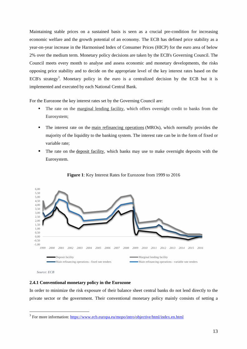
For the Eurozone the key interest rates set by the Governing Council are:

The rate on the marginal lending facility, which offers overnight credit to banks from the

Eurosystem;

The interest rate on the main refinancing operations (MROs), which normally provides the

majority of the liquidity to the banking system. The interest rate can be in the form of fixed or

variable rate;

The rate on the deposit facility, which banks may use to make overnight deposits with the

Eurosystem.

Figure 1: Key Interest Rates for Eurozone from 1999 to 2016

2.4.1 Conventional monetary policy in the Eurozone

In order to minimize the risk exposure of their balance sheet central banks do not lend directly to the

private sector or the government. Their conventional monetary policy mainly consists of setting a

3 For more information: https://www.ecb.europa.eu/mopo/intro/objective/html/index.en.html

Source: ECB

-1,00

-0,50

0,00

0,50

1,00

1,50

2,00

2,50

3,00

3,50

4,00

4,50

5,00

5,50

6,00

1999 2000 2001 2002 2003 2004 2005 2006 2007 2008 2009 2010 2011 2012 2013 2014 2015 2016

Deposit facility Marginal lending facility

Main refinancing operations - fixed rate tenders Main refinancing operations - variable rate tenders

https://www.ecb.europa.eu/mopo/intro/objective/html/index.en.html

14

target for the overnight interbank interest rate and managing the liquidity supply through open market

operations.

The main instruments used by the ECB are:

Reserves: banks are obligated to hold 2 % of their liabilities as a deposit with the Eurosystem

(on average during a month);

Standing facilities (deposit facility and marginal lending facility setting by the ECB) can be

used automatically on the initiative of the banks;

Main refinancing operations (MROs): liquidity provided on a weekly basis to the banks.

MROs are used to control short-term interest rates, to manage the liquidity and to signal the

monetary policy stance in the euro area;

Long–term refinancing operations (LTROs): liquidity provided for a period of 3 months at

market. LTROs provide additional, longer-term refinancing to the financial sector;

Fine–tuning operations: to deal with unexpected surpluses/shortages in the money market.

The weekly decisions taken by the ECB on monetary policy focus on allotment of MROs. The bids are

collected every Monday by the National Central Banks and they are afterwards forwarded to the ECB.

Every Tuesday morning the decision is made by the ECB on the size of the allotment (not on the

minimum bid rate).

2.4.2 Unconventional monetary policy in the Eurozone

During abnormal times, conventional monetary policy instruments may prove insufficient to achieve

the central bank’s objective. Mostly due to the fact that some economic shocks are so powerful that the

nominal interest rate needs to be brought down to zero (Pattipeilohy et al., 2013). At that level, any

additional monetary stimulus it is called unconventional monetary policy and can be achieved in three

complementary ways:

- by guiding medium to long term interest rate expectations;

- by changing the composition of the central bank’s balance sheet (credit easing);

- by expanding the size of the central bank’s balance sheet (quantitative easing).

Unconventional monetary policies can be defined as a class of operations that use the central bank’s

balance sheet in order to directly affect a broader set of market rates, asset prices and even lending

amounts. As such, they represent an attempt to short-circuit and/or enhance the usual transmission

from money market rates into financial conditions facing the wider economy (Meier, 2009).

“QE may work, but it is not a panacea.” (Meier, 2009)

15

Even though according to theory unconventional operations may work the truth is that unconventional

monetary policy involves even more uncertainty than conventional about the economic impact of

some operations (Meier, 2009). In that sense, it becomes important to observe the impact of

unconventional monetary policy.

The non-standard monetary measures applied by the ECB from 2009 until now are:

- Extra liquidity-providing long term refinancing operations;

- Target longer-term refinancing operations;

- Asset purchases programmes;

- Low/negative deposit facility rate4.

2.4.2.1 Description of the ECB unconventional monetary policy announcements

In this section, I will briefly describe the main unconventional policy announcements of the ECB used

in this research from 2009 until 2016.

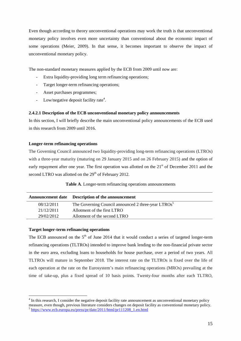
Longer-term refinancing operations

The Governing Council announced two liquidity-providing long-term refinancing operations (LTROs)

with a three-year maturity (maturing on 29 January 2015 and on 26 February 2015) and the option of

early repayment after one year. The first operation was allotted on the 21st of December 2011 and the

second LTRO was allotted on the 29th of February 2012.

Table A. Longer-term refinancing operations announcements

Announcement date Description of the announcement

08/12/2011 The Governing Council announced 2 three-year LTROs5

21/12/2011 Allotment of the first LTRO

29/02/2012 Allotment of the second LTRO

Target longer-term refinancing operations

The ECB announced on the 5th of June 2014 that it would conduct a series of targeted longer-term

refinancing operations (TLTROs) intended to improve bank lending to the non-financial private sector

in the euro area, excluding loans to households for house purchase, over a period of two years. All

TLTROs will mature in September 2018. The interest rate on the TLTROs is fixed over the life of

each operation at the rate on the Eurosystem’s main refinancing operations (MROs) prevailing at the

time of take-up, plus a fixed spread of 10 basis points. Twenty-four months after each TLTRO,

4 In this research, I consider the negative deposit facility rate announcement as unconventional monetary policy

measure, even though, previous literature considers changes on deposit facility as conventional monetary policy. 5 https://www.ecb.europa.eu/press/pr/date/2011/html/pr111208_1.en.html

https://www.ecb.europa.eu/press/pr/date/2011/html/pr111208_1.en.html

16

counterparties have the option to repay any part of the amounts they were allotted in that TLTRO at a

six-monthly frequency.6

Table B. Target longer-term refinancing operations announcements


05/06/2014 The Governing Council decided to conduct a series of TLTROs.

29/07/2014 ECB publishes legal act relating to TLTRO (I)

16/09/2014 Announcement of the first TLTRO (I)

18/09/2014 The ECB allots €82.6 billion in first TLTRO

09/12/2014 Announcement of the second TLTRO (I)

11/12/2014 The ECB allots 129.8 billion in second TLTRO (I)

17/03/2015 Announcement of the third TLTRO (I)

19/03/2015 The ECB allots 97.8 billion in third TLTRO (I)

16/06/2015 Announcement of the fourth TLTRO (I)

18/06/2015 The ECB allots 73.7 billion in fourth TLTRO (I)

22/09/2015 Announcement of the fifth TLTRO (I)

24/09/2015 The ECB allots 15.5 billion in fifth TLTRO (I)

09/12/2015 Announcement of the sixth TLTRO (I)

11/12/2015 The ECB allots 18.3 billion in sixth TLTRO (I)

10/03/2016 The ECB announced new series of TLTROs (II).

22/03/2016 Announcement of the seventh TLTRO (I)

24/03/2016 The ECB allots 7.3 billion in seventh TLTRO (I)

03/05/2016 ECB publishes legal act relating to the new series of TLTROs (II)

Securities markets programme

The Securities Markets Programme (SMP) was meant to buy particular assets (government bonds

from “troubled” countries) in order to repair the monetary transmission channel in the euro area. The

SMP ended in September 2012 but it was replaced by another programme entitled Outright Monetary

Transactions (OMT). This program consists of purchasing unlimited amounts of sovereign bonds of

member states subject to a European Stability Mechanism (ESM) 7 programme on secondary markets.

OMT is aimed as a pure ‘credit easing’ which means that the purchases of government bonds (with

one to three years maturity) in secondary market would just change the assets composition of the

central banks. The OMT programme was announced at the same time as the president of the ECB

(Mario Draghi) announced to do “whatever it takes to save the euro”.

6 http://www.ecb.europa.eu/press/pr/date/2014/html/pr140605_2.en.html

7 The European Stability Mechanism (ESM) is an intergovernmental organization that operates as a permanent

firewall for the euro zone in order to safeguard and provide instant access to financial assistance programmes for

member states of the euro zone in financial difficulty, with a maximum lending capacity of €500 billion.

http://www.ecb.europa.eu/press/pr/date/2014/html/pr140605_2.en.html

17

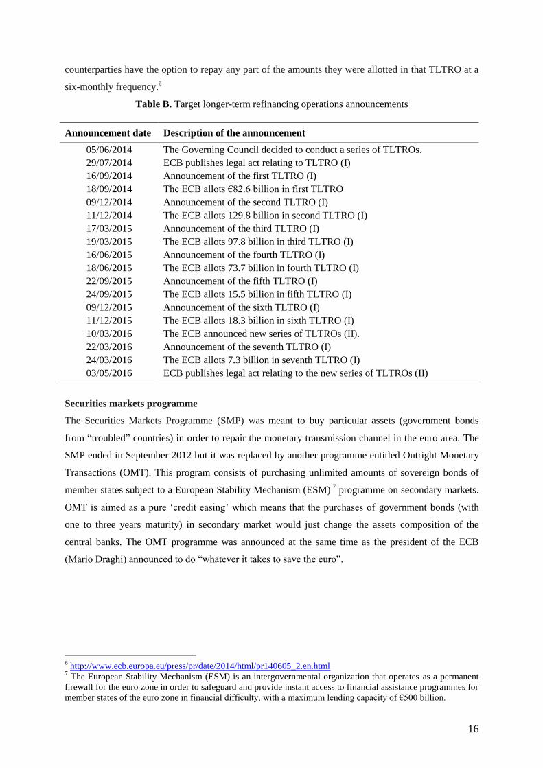
Table C. Securities market programme announcements

To activate the OMT program towards a specific country four conditions have to be met. First, the

country must have received financial support from the European Stability Mechanism (ESM). Second,

the government must comply with the reform efforts required by the respective ESM program. Third,

the OMT program can only start if the country has regained complete access to private lending

markets. Fourth, the country’s government bond yields are higher than what can be justified by the

fundamental economic data. Due to the fact that any country in the group of eligible states for OMT

support did not meet the requirements, the programme has not been activated yet. (Acharya et al.,

2015).

Covered bond purchase programmes (CBPP, CBPP2 and CBPP3)

Covered bonds are bonds issued by credit institutions, which are secured by a protected group of high-

quality assets (such as mortgage loans or public sector debt). Covered bonds grant the holder

privileged claims on the pool of cover assets upon default of the issuer. As a result of these

advantages, covered bonds have proved enormously successful in Europe and they have become a key

source of funding for European banks. More than 80% of the total of covered bond outstanding

globally belongs to six EU countries (Germany, Spain, Denmark, France, Sweden and the UK).

Since the financial crisis started in 2008 investors have been switching preferences towards less risky

assets such as government bonds. This means that covered bonds became less attractive. In order to

prevent the covered bond market from failing the ECB decided to purchase 60 billion euro covered

bonds. The programme was fully implemented on the 30th of June 2010. According to the ECB

9, the

aim of the CBPP has been to support a specific financial market segment that is important for the

funding of banks and that had been particularly affected by the financial crisis. As the euro area did

not recover from the sovereign crisis by 2011, the ECB decided to launch a new covered bond

purchase programme (CBPP2) on 6th of October 2011. The purchases consisted out of 40 billion of

euro-denominated covered bonds in both the primary and the secondary markets.

8 http://www.ecb.europa.eu/press/pr/date/2011/html/pr110807.en.html

9 https://www.ecb.europa.eu/press/pr/date/2010/html/pr100630.en.html


09/05/2010 The ECB announced the SMP

14/05/2010 The ECB published the decision on the SMP

07/08/2011 The Governing Council decided to relaunch the SMP after a period of

inactivity 8

06/09/2012 The SMP ended and the OMT started. Decisions on a number of technical

features regarding the OMT in secondary sovereign bond markets

http://www.ecb.europa.eu/press/pr/date/2011/html/pr110807.en.html

https://www.ecb.europa.eu/press/pr/date/2010/html/pr100630.en.html

18

Table D. Covered bond purchase programme announcements


07/05/2009 The ECB decided to purchase euro-denominated covered bonds issued in

the euro area (CBPP1)

02/07/2009 The ECB started with the purchases of covered bonds (CBPP1)

30/06/2010 The CBPP1 ended (ECB reached the amount purchased of 60 billion)

06/10/2011 The ECB decided to start the second CBPP

03/11/2011 The ECB started with the purchases of covered bonds (CBPP2)

31/10/2012 The CBPP2 ended (ECB reached the amount purchased of 16.4 billion)

Expanded asset purchase programme (APP)

On the 22nd

of January 2015,10

the Governing Council of the ECB decided to launch an expanded asset

purchase programme (APP). It consists of a third covered bond purchase programme (CBPP3), an

asset-backed securities purchase programme (ABSPP) and a public sector purchase programme

(PSPP). The latter is a completely new programme for the ECB. So far, the ECB has been only buying

assets from the private sector.

In order to fight the risks of a too prolonged period of low inflation the ECB started buying public

sector securities on 9th March 2015. The securities covered by the PSPP include nominal and inflation-

linked central government bonds and bonds issued by recognized agencies, international organizations

and multilateral development banks located in the euro area. The expanded asset purchase programme

is expected to be carried out until September 2016 and in any case until the Governing Council sees a

sustained adjustment in the path of inflation. Combined monthly purchases in public and private sector

securities will amount to €60 billion. On the 3rd

December 2015 the ECB announced an extension of

the APP until March 2017 and an increase in the monthly purchase up to EUR 80 bn. On the 20th of

October 2014, the Eurosystem started to buy covered bonds under a third covered bond purchase

programme (CBPP3). The ABSPP started on 21 November 2014 and consists out of purchasing in

both primary and secondary markets senior and guaranteed mezzanine tranches of asset-backed

securities (ABSs).

Table E. Expanded asset purchase programme announcements


04/09/2014 The ECB announced a new CBPP (3) and a new ABSPP

20/10/2014 The ECB started to buy covered bonds (CBPP3)

21/11/2014 The ECB started the ABSPP

22/01/2015 The ECB announced the expanded asset purchase program.

09/03/2015 The ECB started to buy public sector securities under the PSPP

18/03/2015 The Governing Council decided on the criteria for which mezzanine

10



19

tranches of ABS would be considered for purchase under the ABSPP

Corporate Sector Purchase Programme

The Corporate Sector Purchase Programme (CSPP) is a new programme that has been added to the

existing elements of the asset purchase programme (APP). According to the ECB11

, the CSPP aims to

purchase investment-grade euro-denominated bonds issued by non-bank corporations established in

the euro area. It will be included in the combined monthly purchases that increased on the 1st of April

2016 to €80 billion.

Table F. Corporate sector purchase programme announcements


10/03/2016 The ECB added the CSPP to the APP

21/04/2016 The ECB announced details of the CSPP

08/06/2016 The ECB started CSPP

Negative deposit facility rate

The deposit facility rate is one of the three interest rates that the ECB sets every six weeks as part of

its monetary policy. The rate defines the amount of interest the banks receive for depositing money at

the central bank overnight. Since the 11th

of June 2014, this rate has been negative12

. The 11th of June

2014 was the first time in the Eurozone that the Governing Council of the ECB set the deposit facility

rate negative. Following the ECB’s example, Sweden set negative nominal interest rates combined

with bond buying; Denmark and Switzerland also cut their nominal interest rates below zero in order

to protect the currency’s peg to the euro (Warner, 2015).

Table G. Negative deposit facility rate announcements


05/06/2014 The Governing Council announced for the first time that the deposit facility

rate would be below zero (-0.10)

11/06/2014 The ECB started applying the -0.10 deposit facility rate.

04/09/2014 The Governing Council set deposit facility rate even more negative (-0.20)






11

https://www.ecb.europa.eu/press/pr/date/2016/html/pr160310_2.en.html 12

https://www.ecb.europa.eu/explainers/tell-me/html/what-is-the-deposit-facility-rate.en.html


https://www.ecb.europa.eu/explainers/tell-me/html/what-is-the-deposit-facility-rate.en.html

20

3. Literature Review

In this chapter, I introduce some of the literature that has been conducted on unconventional monetary

policy by the ECB and also by another central banks (e.g. Bank of Japan, Bank of England and

Federal Reserve).

3.1 Previous literature on the effect of unconventional monetary policy in the euro area

Eser and Schwaab (2013) tested the yield impact of the Securities Market Programme launched by

ECB on the 14th May 2010. Even despite the sovereign debt crisis, they show that government bond

purchases during the SMP were effective in affecting yields for Spain, Italy, Ireland, Portugal and

Greece (also known as PIIGS). One of their aims during their research was to estimate how long the

effects were going to last. They found evidence for both transitory and long-run effects.

Falagiarda and Reitz (2015) studied the effects of ECB announcements regarding unconventional

monetary policy operations on the sovereign spreads of Greece, Ireland, Italy, Portugal, and Spain

relative to Germany between 2008 and 2012. Their results showed that ECB unconventional monetary

policy announcements reduced long-term government bond yield spreads substantially relative to

German counterparts in all countries, except for Greece. In particular, they found that news about the

Securities Markets Programme strongly affected the “PIIGS”, while the Outright Monetary

Transactions announcements only had a significant impact in Italy and Spain.

Brand et al. (2010) wanted to study the impact of central bank communications and decisions on the

yield curve by using high frequency data on money market interest rates. They affirmed that market

expectations of the path of monetary policy might change considerably during the ECB’s press

conference and that these changes have a considerable impact on longer-term yields. Additionally,

their results show that news coming from ECB communication matter more for long-term interest

rates than news about actual monetary policy decisions.

The ECB Economic Bulletin (2015)13

presented an article that evaluates the transmission of the ECB’s

non-standard measures announced. It focuses on the targeted longer-term refinancing operations

(TLTROs), the expanded asset purchase programme (APP) and on the public sector purchase

programme (PSPP). The results suggested that these policies together had significantly lowered yields,

with the effects generally increasing with maturity and riskiness. For instance, ten-year yields declined

by about 70 basis points for the euro area. They used inflation swap rates as a measure of the private

sector’s inflation expectations for maturities between one and five years. The estimated change in

inflation swap rates due to the APP is around 30 basis points for the one-year maturity and around 20

basis points for the five-year maturity.

13

https://www.ecb.europa.eu/pub/pdf/other/eb201507_article01.en.pdf

https://www.ecb.europa.eu/pub/pdf/other/eb201507_article01.en.pdf

21

3.2 Previous literature on the effect of unconventional monetary policy on other central banks:

USA, Japan and England

Bank of Japan

Berkmen’s (2012) paper assesses the impact of quantitative easing in Japan on economic activity and

inflation during 1998-2010. Instead of using government bond spreads as a proxy for QE, the author

measures the effectiveness of asset purchasing programs through the following four variables: the

economic activity variable (growth or unemployment rate), the inflation, the interest rate and the

government bond spread over the policy rate. The paper finds some evidence that monetary easing by

the Bank of Japan has supported economic activity, even though the statistical significance varies

according to the different measures used for economic activity. Furthermore, there is no evidence of

an impact on the exchange rate and the effect on inflation is weak.

Lam (2011) measured the impact of the new asset purchase program under the Bank of Japan’s

Comprehensive Monetary Easing (CME)14

on financial markets. An event study approach is used

where the author analyses how financial markets responded to the announcement of the QE by the

Bank of Japan, whether the impact comes mostly from the first announcement of the QE or the

subsequent QE and which asset purchases, private risky assets or government securities, are more

effective in reducing risk premia. He concludes that easing measures used by the Bank of Japan had a

statistically significant impact on bond yields and equity prices, but no outstanding effect on the

exchange rate and inflation expectation. Moreover, Lam concluded that the impact arises from the

announcement effect rather than from the actual operations or purchases. Lam (2011) went further and

analysed the hypothetical scenario of the impact on financial markets if CME had not included private

asset purchases. He concludes that including private risky assets in the program is a crucial factor to

support asset prices.

Honda et al. (2013), based on a VAR methodology, examine the effect of the QE on aggregate output

and prices and its transmission channel. They look at the effects of the QE in Japan from 2001-2006.

They concluded that any additional injection of money is effective even when short-term nominal

interest rates are zero. However, there is no impact on the price level. In order to test the transmission

channel, they considered the following financial variables: short-to long term nominal interest rates,

stock prices, foreign exchange rates and bank lending. From these variables, they concluded that QE

increased aggregate output through the stock price channel. Hence, a QE shock first raises stock prices

and then increases the output level. They also found empirical evidence that people did not spend

14

According to Lam (2011), “Comprehensive Monetary Easing (CME) differs from the typical quantitative

easing in other central banks by including purchases of risky assets in an effort to reduce term and risk premia.”

22

money to purchase bonds, which is consistent with the liquidity trap theory. On the contrary, they find

that people use the injected money to purchase stocks.

Federal Reserve

Gagnon et al. (2011) used an event-study analysis of Federal Reserve communications to obtain the

effect of Large-Scale Asset Purchases Program (LSAP). They examine changes in the following

financial variables around the official communications of asset purchases: 2-year and 10-year Treasury

yields, the 10-year agency debt yield, the current-coupon 30-year agency MBS yield, the 10-year

Treasury term premium, the 10-year swap rate, and the Baa corporate bond index yield. They conclude

that the Federal Reserve’s LSAP programs were successful at lowering longer-term private borrowing

rates and stimulating economic activity. However, the agency debt yield and the MBS yield changed

very little. Moreover, they found evidence of LSAPs broader effects. Swap rate and the Baa corporate

bond yield also decreased significantly.

D’Amico and King (2010) investigated the effects of LSAP conducted by Fed on yields. They

conducted a panel of daily CUSIP-level data. Their results suggested that, on average, LSAP reduced

yields by about 30 basis points across the yield curve during the life of the program. The effects were

most pronounced in securities with 10 to 15 years of maturity. They estimated that these yields would

have been 50 basis points higher in the absence of the program. They also found that the decreases on

yields are generally higher for the specific securities being bought and for securities of similar

maturities.

Neely (2010) also followed an event study methodology that evaluates the impact of Federal Reserve’s

unconventional monetary policy on long term bond yields. However, he brought something new to the

current literature, by also estimating the impact on nominal international long bond yields in local

currencies and exchange rates. The unconventional policies significantly reduced the 10-year nominal

yields for Australia, Canada, Germany, Japan and the United Kingdom. The USD also depreciated

against the currencies of those countries.

Krishnamurthy and Vissing-Jorgensen (2010) analyse the effect of Federal Reserve's purchase of long

term Treasuries and other long-term bonds on nominal and real long-term interest rates. In order to do

that they designed an event study based on the announcements dates of long-term asset purchases by

the Federal Reserve in the late 2008 to 2009 period. They find a large and significant decrease in

nominal interest rates on long-term safe assets (Treasuries and Agency bonds). Additionally, they

conclude that both QE (1 and 2) had a smaller effect on less safe assets, such as Baa corporate rates

and mortgage rates. They believe the reason behind that is the fact that Baa corporate rates and

mortgage rates are more relevant for corporate and households long-term borrowing. According to

23

Krishnamurthy and Vissing-Jorgensen (2010), the type of asset purchased by the central bank matters

for the final outcome, as well as, the type of interest rate being used to test the impact of the asset

purchases. Besides, as most of the economy is funded by debt (not risk free as government bonds)

observing effects on government bonds might be misleading (Krishnamurthy and Vissing-Jorgensen,

2010). Therefore, I decided to investigate the effect not only on government bond yield but also on

corporate bond yields (AAA and BBB). Krishnamurthy and Vissing-Jorgensen (2010) used agency

bonds to measure the impact of asset purchases. During QE1 the agency yields decrease 164 basis

points and the Agency MBS yields fall by 116 basis points. Furthermore, they use information from

inflation swap rates and they find evidence that expected inflation increased as a result of the first QE

(increased 71 basis points), but it did not change a lot as a result of the second QE.

Wright (2012) also provides evidence that asset purchases conducted by Fed decreased long-term

interest rates. Although the impact is statistically significant, the effect fades rapidly over the

subsequent months. He uses a structural VAR method15

with daily data to measure the effects of

monetary policy on long-term interest rates since the moment the federal funds rate has been stuck at

the zero lower bound. By using the same methodology as Rigobon (2003) and Rigobon and Sack

(2003, 2004, 2005) the author concludes that monetary policy shocks have effects on both long term

Treasury and corporate bond yields. The results show that quantitative easing (QE1, QE2 and QE3)

declines interest rates, but that these are reversed over the subsequent months. However, it is not

certain whether the result come from the economic stimulus provided by the Federal Reserve action

(QE) or whether it was because the markets overreacted to the announcement of the quantitative

easing.

According to theory, ultra-low rates could boost equity prices in the long term, all else being equal.

For example, by lowering the discount rate that investors use they could anticipate an increase in the

present value of future cash flows, which should boost the stock-market valuation. Another

explanation might be that as yields on fixed-income securities decline, investor may shift into equities

and other assets in search of higher yields, increasing demand for these assets and therefore their

prices (Koller, Dobbs & Lund, 2014). However, according to Koller, Dobbs and Lund (2014) the

impact on equity prices might not be significant. In their paper, they mentioned that could happened

due to “rational expectations”. As the investors take today’s ultra-low rate as temporary, the discount

rate used to value future cash flows is not going to be reduced in the future. The second reason that

they mentioned is that if investors had reduced their discount rate in the future we would expect P/E

ratios to rise. However, the last years P/E ratios have remained constant.

15

The structural VAR uses economic theory to sort out the contemporaneous links between variables. It requires

identifying assumptions that allow correlations to be interpreted causally (Stock and Watson, 2001).

24

Bank of England

In March 2009, the Bank of England began a quantitative easing programme. Joyce at al. (2010)

intended to verify the impact of those large purchases of assets on financial markets. They conducted

an event study method that focused on the reaction of the market prices over a fairly narrow interval

after the QE-related news was announced. Their goal is to capture the market’s response to the news,

isolated from other factors that may also have been affecting asset prices. According to the authors,

there are three main channels through which QE might affect prices: the macro/policy news channel,

portfolio-rebalancing channel and the liquidity premia channel. Their analysis suggests that there was

a decrease on gilt yields (about 100 basis points lower) due to the QE announcements mainly through

a portfolio rebalancing effect.

Meier (2009) through an event study concludes that the quantitative easing programme conducted by

the Bank of England was “moderately encouraging”. He found evidence of a direct impact on gilt

yields. Moreover, the asset purchases of the Bank of England have coincided with a recovery of asset

prices, a decline in risk spreads and a moderate increase in breakeven inflation rates. On the other

hand, he also found that the sterling pound has gradually appreciated since the launch of the QE,

which is against the theory.

Zhu and Meaning (2011) investigated the effectiveness of the asset purchase programmes

implemented by the Federal Reserve (LSAP)16

and the Bank of England (APF)17

. They used two

different methodologies. First, they used an event study based on the Gagnon et al. (2011)

methodology in which they conclude that the impact was significant to the first announcements but

really small to the announcements of latter extensions of the programmes. Secondly, they used the

methodology of D’Amico and King (2010) and they found that yields fell significantly over the course

of each programme (which matches with the results from the first method). They found that on a one-

day event window the asset purchase programmes announcements significantly reduced yields of

government bonds yields and that the prices of some risky assets increased as the programmes were

announced. There was also a sizeable reduction in corporate bond yields. The first announcements

preceded significant depreciations in the nominal effective exchange rates of the US dollar and

sterling. However, the impact was little for the later programmes. They conclude that recent asset

purchases seem to have been effective, but there are limitations for further actions. Firstly, long-term

government bond yields are already very low and the scope for further reduction becomes smaller as

more purchases are carried out. Secondly, it may be difficult to achieve the same degree of

16

Federal Reserve’s Large-Scale Asset Purchase 17

Bank of England’s Asset Purchase Facility

25

effectiveness as with the initial programmes once the surprise or novelty element fades. Lastly, central

banks face some risks with large holdings of longer-term securities and riskier private debt.

Breedon, Chadha and Waters (2012) studied the impact of the first quantitative easing programme

conducted by the Bank of England (from March 2009 to February 2010) on asset prices. They

estimated a simple term structure model driven by several macroeconomics factors. Then, they used

this model to estimate a predicted yield curve over the QE period. The difference between the

predicted and the actual yield curve over the QE period can be interpreted as an estimate of the

portfolio balance impact of QE. Breedon, Chadha and Waters (2012) wanted to observe the spillover

effects from the QE on the US forward interest rates18

. They followed the same announcement effect

methodology as Gagnon et al. (2011), where they examined both the 1-day and the 2-day changes,

which were measured from the day before the FED announcement and the day after the

announcement. During the QE programme, there were eight federal open market committee

statements. They found out that the impact on US forward interest rates varies depending on maturity

and the size of the announcement window. Moreover, they concluded that QE is indeed effective in

influencing long-term bond yields through a portfolio balance effect. However, the broader impact of

QE on other assets and on the economy remains controversial. Mainly due to the fact that QE has been

implemented during a credit crunch, which does not allow to distinguish the impact of conventional

measures from unconventional (Breedon, Chadha & Waters, 2012).

Kapetanios et al. (2012) observed the impact on output and inflation of QE conducted by the Bank of

England. They had to carry out a counterfactual analysis of what would have happened to GDP and

inflation if QE had not been implemented. After that, the difference between the counterfactual and

the baseline prediction (when QE happens) is the measure of the macroeconomic impact. Their results

suggested that without QE inflation would have been low or even negative and real GDP would have

fallen even more. Likewise, Gambacorta et al. (2012) carried out a cross country analysis to find the

impact on the macro economy during the financial crisis. They estimated a panel structural vector

autoregressive (SVAR) model with monthly data over a sample period. The countries included in the

analysis were Canada, the euro area, Japan, Norway, Sweden, Switzerland, the United Kingdom and

the United States. They concluded that expansions of the central banks’ balance sheet lead to a

significant but at the same time temporary rise in output and prices. The impact on the price level

appears to be less persistent and weaker. Their results demonstrated that unconventional monetary

policy measures used by central banks in the wake of the global financial crisis provided temporary

support to their economies.

18

Forward interest rate can be viewed as the rate set at time t on a contract to purchase a bond at time t +

1,2,3,… (Fama and Bliss, 1987 )

26

4. Data

The data set considered in this study includes daily long term interest rates for 11 out of 19 countries

that have the euro as their physical currency since 2002 (Austria, Belgium, Germany, Greece, Finland,

France, Ireland, Italy, Netherlands, Portugal and Spain). The long-term interest rates considered in this

research are the 10-year on-the-run government benchmark bond yields. They were collected from

Datastream. Thomson Reuters Datastream compiles the benchmark yield data from the central bank of

each country. These on-the-run government benchmark yields have already been used in previous

literature as a measure of long-term interest rates (e.g. Carvalho & Fidora (2015) and Falagiarda &

Reitz (2015)). While applying the market model to compute the expected return, the synthetic Euro

benchmark bond was used as the “market return”. It consists out of a weighted average yield of the

benchmark bond series from each European Monetary Union member mentioned above19

.

To evaluate the impact on other securities different from government bonds, corporate bond yield data

is also considered in this research. A 10-year and 5-year benchmark on corporate bond yields is

utilized for two different types of credit ratings: AAA (prime) and BBB (lower medium grade). The

data was collected from Datastream for the Eurozone.

In order to measure the medium term inflation expectations, it is employed the Euro Inflation Swap

Forward 5y5y. It measures expected inflation (on average) over the five-year period that begins five

years from today. This rate is used by central banks to get information on the market’s future inflation

expectations. The swaps are traded daily. The data on Euro Inflation Swap Index was collected from

Bloomberg for the Eurozone.

The dataset starts on the 1st of March 2009 and ends on 5

th of July 2016. The number of

unconventional monetary policy announcements that occurred during that period were 44. Two of the

announcements were made on a Sunday (07/08/201120

and 09/05/201021

). As there are no yield data

on weekends, I decided to place them on the Monday. In order to be able to capture the impact of each

announcement, I removed the announcements that followed each other within 30 days. Hence, the

final number of announcements accounts to 22.

19 The weightings used are the 1996 real GDP as published by Eurostat. The precise formula is the following:

20 The Governing Council decided to relaunch the SMP after a period of inactivity.

21 The ECB announced the Securities Markets Programme (SMP).

27

5. Methodology

The focus of the present research is to evaluate the impact of ECB unconventional monetary policy on

long-term interest rates (10-year government bond yield) for the following euro area countries:

Austria, Belgium, Germany, Greece, Finland, France, Ireland, Italy, Netherlands, Portugal and Spain.

Furthermore, the impact of ECB non-standard measures is also going to be tested on inflation

expectations and on corporate bond yields for the Eurozone. The way to conduct this study is by using

an event-study.

5.1 Event study

The event study methodology allows to evaluate whether movements of a time series around a certain

date are consistent with normal returns or if they can be considered abnormal in a statistically

significant way. Event study methods were first developed in the financial economics literature,

originally introduced by Eugene Fama, Lawrence Fisher, Michael Jensen and Richard Roll in the

paper “The Adjustment of Stock Prices to New Information” in 1969, as a method to test the efficient

markets hypothesis using the analysis of returns around an unanticipated event (Sandler & Sandler,

2012).

The event study approach relies on the efficient market hypothesis and also on the rational expectation

hypothesis, by which prices and returns incorporate all the information available. Thus, long term

interest rates should react to announcements regarding unconventional monetary policy because

expectations are being affected by those announcements (Rivolta, 2014).

When using an event study it is implicitly assumed that the event set includes all announcements that

have affected expectations about the future of monetary policy; monetary policy expectations have not

been affected by anything other than these announcements; responses can be measured in windows

wide enough to capture long-run effects but not so wide that information affecting yields through other

channels is likely to have arrived and markets are efficient in the sense that all the effects on yields

occur when market participants update their expectations and not when actual purchases take place

(Gagnon et al., 2011).

There are some disadvantages associated with the event study methodology. The assumptions

mentioned above are very strong and if misused can bias the results of a research. It is impossible to

control for other factor(s) that occur at the same time. In order to make sure that these flaws do not

influence the results of this research, I decided to analyse the yield changes in a narrow interval of

time around each announcement. Moreover, I selected a control period (estimation window) that does

28

not include the event window. To do be able to do that, I had to exclude unconventional monetary

policy announcements following each other within 30 days.

In this research, an event-study analysis of the ECB monetary policy announcements will be used to

estimate the effects of monetary policy implemented between May 2009 and June 2016. In particular,

changes in nominal and real long-term yields (10-year government bond yields, 5y5y swap forward

rate and corporate bond yields) around official communications on unconventional monetary policy

are going to be examined, by taking the cumulative changes as a measure of the overall effects.

To conduct an event study, an event window and estimation window were selected. The day of the

announcement is the event day and therefore, it is defined as t=0. However, I am not only interested on

the yield changes on the day of the announcement itself but also on the days surrounding the event

day. Selecting the window length involves a trade-off between allowing sufficient time for revised

expectations to become fully incorporated in asset prices and keeping the window narrow enough to

make it unlikely to contain the release of other important information (Gagnon et al., 2011). Following

Gagnon et al. (2011), I considered a two day window, [-1,0] and [0,1], around the announcements. A

two day window measures the day prior (or after) to the announcement until the closing day of the

announcement. The two day window [0, 1] allows for the fact that it can take some time before the

market adapts to the announcements of the ECB. Also, [-1,0] allows for the fact that investors have

rational expectations and they can anticipate then announcement22

. Furthermore, I also use a three day

window [−1,+1]. There is no uniform agreement on the estimation period (Sorokina et al., 2013). I

selected an estimation window of 30 days. As the estimation window should be defined prior to the

event window, the control period for this event study is [-32,-2]. Doing so guarantees that the event

period is not included in the estimation period which prevents the results of being influenced by the

returns around the event (Mackinlay, 1997).

The calculation of the event's impact requires measuring abnormal returns. In this particular research,

the “returns” are abnormal yield changes. The abnormal yield change is the actual ex post change of

the yield over the event window minus the normal yield change over the event window (Mackinlay,

1997). The normal yield change is the expected yield change in case no event had occurred. The

abnormal yield change can be calculated as follows:

(4)

where means period of time and country.

22

According to the rational expectations theory efficient markets react to a policy measure in anticipation of its

actual implementation.

29

To obtain the expected yield change the following models can be reviewed:

- Constant mean return model

- CAPM

- Arbitrage pricing theory

- Market model

In this study two models were applied. The constant mean return model and the market model. The

first model assumes that expected returns can differ by country, but are constant over time. The

formula of the expected yield change according to constant mean return model is as follows:

(5)

where is the mean of the yield changes on the estimation window per period- and country ( ).

The market model consists out of a statistical model that relates the return of any given security to the

return of the market portfolio (Mackinlay, 1997). In this research, the market model relates the yield

change of each country to the weighted average yield of the benchmark bond series from each

European Monetary Union country. According to the market model, the formula of the expected yield

change can be write as follows:

(6)

where is a weighted average yield of the Eurozone yields23

, and is the zero mean disturbance

term. and are the parameters of the market model.

After calculating the expected normal yield change the abnormal yield change can be calculated as

follows:

(for the constant mean return model) (7)

(for the market model) (8)

where designates the actual yield change.

In order to measure the total impact of the announcement within the event window, the cumulative

abnormal yield change has to be calculated. The cumulative abnormal yield change (CAYC) is the

sum of the abnormal yield changes over a certain period around the event. For instance, if I consider

23

The formula can be found in chapter 4 (Data).

30

the three day event window [-1,1]. The respective CAYC is just the sum of the abnormal yield

changes on the day before the event, the event day itself and the day after the event.

∑ (9)

5.2 Statistical significance

After calculating the abnormal yield change and cumulative abnormal yield change their significance

needs to be tested. Therefore, I compute a t-test statistic to check whether the average abnormal yield

change for each country used in the event study are statistically different from zero. Under the null

hypothesis, the cumulative abnormal average yield change is equal to zero. This means that if the null

hypothesis is not rejected, yields remained unchanged after the announcements of unconventional

monetary policy. Opposite to that, the alternative hypothesis states that the cumulative abnormal

average yield is different than zero.

In order to test the null hypothesis, the following t-test is conducted:

∑

⁄

√ ⁄

⁄

√ ⁄

(10)

where N is the number of days in the event window and is the standard deviation of the abnormal

yield change.

I use a two-sided t-test. Based on the test statistic resulting from (8), I either reject or accept the null

hypothesis. There are three levels of significance (1%, 5% and 10%) at which the null hypothesis can

be rejected. In a two-sided t-test, if then the null hypothesis is reject at 1%

significance level. If then the null hypothesis is rejected at 5% significance level.

Lastly, if then the null hypothesis is rejected at 10%.

31

6. Results

Tables related with the results of the event study can be found in Appendix I to XIII.

If the null hypothesis is rejected, then unconventional monetary policy announcements are having a

positive or negative effect on yields (Sawson, 2011). When the ECB purchases bonds directly, the

total supply of long term bonds available in the market decreases. As the supply of the bonds

decreases, the price of the bonds should rise and the long-term government yields should fall.

Additionally, unconventional monetary policy announcements can have a signaling effect regarding

future monetary policy. However, not all types of unconventional monetary policy announcements

have a clear sign prediction of the yield change. Expectations of easier monetary policy might cause

longer-term nominal interest rates to either rise or fall (Sawson, 2011). For example, when the ECB

cut the deposit facility to greater negative values (on the 10th of September 2014), it could have been

interpreted by the market as a sign that the interest rates would be maintained at a low level for a

longer period. Hence, the nominal long-term interest rates were expected to decrease.

Even though the sign of the yield change might change according to the type of the unconventional

monetary policy announcement, I expect that the ECB announcements will lower nominal long-term

interest rates and, as desired by the ECB, increase inflation expectations.

6.1 Overall effect of the ECB unconventional monetary policy

For both models (the market model and the constant mean return model) and interest rates (10-year

government bond yield, swap forward rate 5y5y and corporate bond yields) considered in this

research, the abnormal yield changes are not significant. Still, some conclusions can be drawn about

them. Both models show that only when t=1 (one day after the announcement), the abnormal yield

changes decreased. This implies that the market might take some time to react to the ECB

unconventional monetary policy announcements.

According to both models (the market model and the constant return model), all the CAYCs, on the

10-year long-term interest rates, are significant at 1% (see tables H and I). The cumulative abnormal

10-year government bond yield change decreased by 3.747 percentage points, during the day and the

day immediately after the announcement [0,1]. Albeit, not all the significant changes in the 10-year

government bond yield are negative (as expected). Therefore, there is evidence that unconventional

monetary policies conducted by the ECB are affecting long-term interest rates significantly, however,

the sign of that impact is not totally clear.

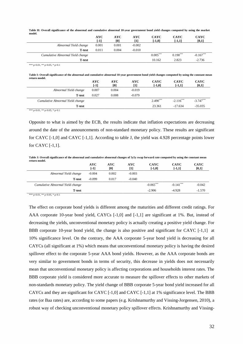
32

Table H: Overall significance of the abnormal and cumulative abnormal 10-year government bond yield changes computed by using the market

model.

AYC

[-1]

AYC

[0]

AYC

[1]

CAYC

[-1,0]

CAYC

[-1,1]

CAYC

[0,1]

Abnormal Yield change 0.001 0.001 -0.002

T-test 0.011 0.004 -0.010

Cumulative Abnormal Yield change

0.005*** 0.190*** -0.167***

T-test

10.162 2.823 -2.736

*** p<0.01, ** p<0.05, * p<0.1

Table I: Overall significance of the abnormal and cumulative abnormal 10-year government bond yield changes computed by using the constant mean

return model.

AYC

[-1]

AYC

[0]

AYC

[1]

CAYC

[-1,0]

CAYC

[-1,1]

CAYC

[0,1]


T-test 0.027 0.008 -0.079


2.490*** -2.116*** -3.747***

T-test

23.361 -17.634 -35.035

*** p<0.01, ** p<0.05, * p<0.1

Opposite to what is aimed by the ECB, the results indicate that inflation expectations are decreasing

around the date of the announcements of non-standard monetary policy. These results are significant

for CAYC [-1,0] and CAYC [-1,1]. According to table J, the yield was 4.928 percentage points lower

for CAYC [-1,1].

Table J: Overall significance of the abnormal and cumulative abnormal changes of 5y5y swap forward rate computed by using the constant mean

return model.

AYC

[-1]

AYC

[0]

AYC

[1]

CAYC

[-1,0]

CAYC

[-1,1]

CAYC

[0,1]

Abnormal Yield change -0.004 0.002 -0.003

T-test -0.099 0.017 -0.040


-0.065*** -0.141*** -0.042

T-test

-2.906 -4.928 -1.570

*** p<0.01, ** p<0.05, * p<0.1

The effect on corporate bond yields is different among the maturities and different credit ratings. For

AAA corporate 10-year bond yield, CAYCs [-1,0] and [-1,1] are significant at 1%. But, instead of

decreasing the yields, unconventional monetary policy is actually creating a positive yield change. For

BBB corporate 10-year bond yield, the change is also positive and significant for CAYC [-1,1] at

10% significance level. On the contrary, the AAA corporate 5-year bond yield is decreasing for all

CAYCs (all significant at 1%) which means that unconventional monetary policy is having the desired

spillover effect to the corporate 5-year AAA bond yields. However, as the AAA corporate bonds are

very similar to government bonds in terms of security, this decrease in yields does not necessarily

mean that unconventional monetary policy is affecting corporations and households interest rates. The

BBB corporate yield is considered more accurate to measure the spillover effects to other markets of

non-standards monetary policy. The yield change of BBB corporate 5-year bond yield increased for all

CAYCs and they are significant for CAYC [-1,0] and CAYC [-1,1] at 1% significance level. The BBB

rates (or Baa rates) are, according to some papers (e.g. Krishnamurthy and Vissing-Jorgensen, 2010), a

robust way of checking unconventional monetary policy spillover effects. Krishnamurthy and Vissing-

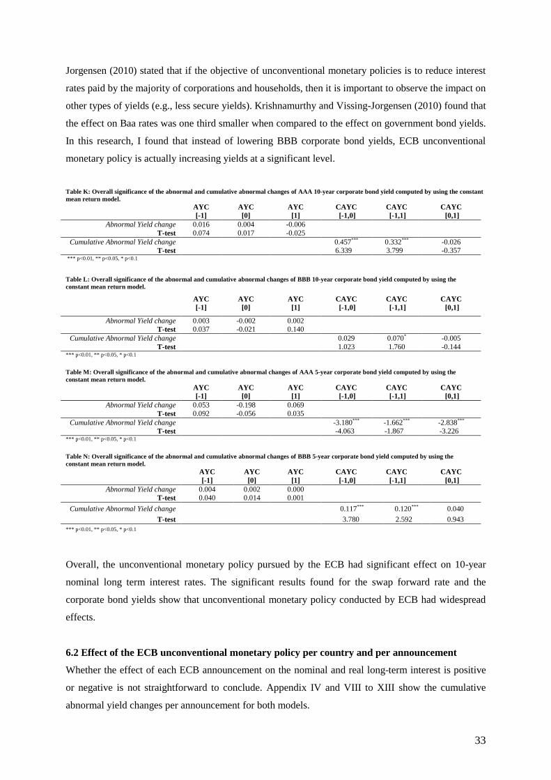
33

Jorgensen (2010) stated that if the objective of unconventional monetary policies is to reduce interest

rates paid by the majority of corporations and households, then it is important to observe the impact on

other types of yields (e.g., less secure yields). Krishnamurthy and Vissing-Jorgensen (2010) found that

the effect on Baa rates was one third smaller when compared to the effect on government bond yields.

In this research, I found that instead of lowering BBB corporate bond yields, ECB unconventional

monetary policy is actually increasing yields at a significant level.

Table K: Overall significance of the abnormal and cumulative abnormal changes of AAA 10-year corporate bond yield computed by using the constant

mean return model.

AYC

[-1]

AYC

[0]

AYC

[1]

CAYC

[-1,0]

CAYC

[-1,1]

CAYC

[0,1]


T-test 0.074 0.017 -0.025

Cumulative Abnormal Yield change 0.457*** 0.332*** -0.026

T-test 6.339 3.799 -0.357 *** p<0.01, ** p<0.05, * p<0.1

Table L: Overall significance of the abnormal and cumulative abnormal changes of BBB 10-year corporate bond yield computed by using the

constant mean return model.

AYC

[-1]

AYC

[0]

AYC

[1]

CAYC

[-1,0]

CAYC

[-1,1]

CAYC

[0,1]

Abnormal Yield change 0.003 -0.002 0.002

T-test 0.037 -0.021 0.140

Cumulative Abnormal Yield change 0.029 0.070* -0.005

T-test 1.023 1.760 -0.144 *** p<0.01, ** p<0.05, * p<0.1

Table M: Overall significance of the abnormal and cumulative abnormal changes of AAA 5-year corporate bond yield computed by using the


AYC

[-1]

AYC

[0]

AYC

[1]

CAYC

[-1,0]

CAYC

[-1,1]

CAYC

[0,1]

Abnormal Yield change 0.053 -0.198 0.069

T-test 0.092 -0.056 0.035


-3.180*** -1.662*** -2.838***

T-test

-4.063 -1.867 -3.226 *** p<0.01, ** p<0.05, * p<0.1

Table N: Overall significance of the abnormal and cumulative abnormal changes of BBB 5-year corporate bond yield computed by using the


AYC

[-1]

AYC

[0]

AYC

[1]

CAYC

[-1,0]

CAYC

[-1,1]

CAYC

[0,1]

Abnormal Yield change 0.004 0.002 0.000

T-test 0.040 0.014 0.001


0.117*** 0.120*** 0.040

T-test

3.780 2.592 0.943

*** p<0.01, ** p<0.05, * p<0.1

Overall, the unconventional monetary policy pursued by the ECB had significant effect on 10-year

nominal long term interest rates. The significant results found for the swap forward rate and the

corporate bond yields show that unconventional monetary policy conducted by ECB had widespread

effects.

6.2 Effect of the ECB unconventional monetary policy per country and per announcement

Whether the effect of each ECB announcement on the nominal and real long-term interest is positive

or negative is not straightforward to conclude. Appendix IV and VIII to XIII show the cumulative

abnormal yield changes per announcement for both models.

34

When the ECB purchases long-term government bonds, the supply decreases. This policy affects

interest rates through a portfolio balance: The ECB reduces the portfolio of long term versus short-

term bonds for the investors and, consequently, lowers long-rates against short rates (Krishnamurthy

and Vissing-Jorgensen, 2010). Even though the results are not significant during the first time that

ECB started buying covered bonds (07/05/2009), they still show that the cumulative abnormal 10-year

government bond yield decreased. Instead, when they decided to start the second purchase of covered

bonds (CBPP2) the cumulative abnormal yield change increased. This might imply that the

effectiveness of the policy declines with each CBPP announcement. After the announcement of the

Securities Market Programme (10/5/2010), the cumulative abnormal 10-year government bond yield

decreased and the inflation expectations increased, significantly, for all CAYCs (at 1% level). The

effect on corporate bond yields is not completely clear in terms of the sign of the yield change and not

significant. The results for the 10-year government bond yield match the findings of Eser and Schwaab

(2013). I also found that yields decreased for the PIIGS countries (Portugal, Ireland, Italy, Greece and

Italy).

Giving the constant mean return model, announcements of LTROs lowered yields for all the CAYCs.

In similar way, the BBB 10-year and 5-year corporate bond yields decreased for almost the entire lot

of LTROs announcements. This outcome shows that the ECB is being effective in reducing nominal

long-term interest rates by targeting longer-term refinancing operations. On the other hand, Appendix

IX shows that during all the TLTROs announcements the 5y5y swap forward rate decreased

significantly, meaning that inflation expectations are also falling with the LTROs announcements.

Following the Expectations Hypothesis, one would expect that when the ECB lowered the deposit

facility rate to negative values, the long term interest rate would consequently fall. The results show

that on the 11th of June 2014, when the ECB started to apply a -0.10 deposit facility, the cumulative

abnormal yield changes increased (not significantly) according to the constant mean return model,

which is not in line with the theory mentioned before. The corporate bond yields also increased for the

same period. Only the expected inflation decreased significantly at 5%. Besides the announcement on

04/09/2014, there was no announcement regarding the deposit facility rate that had led to a negative

yield impact for the 10-year government bonds and for the BBB corporate bond yield.

On the 4th of September of 2014, the ECB announced the new asset-backed securities purchase

programme (ABSPP) and at the same time they lowered the deposit rate facility to historical negative

levels (-0.20). The combination of these two announcements was expected to significantly affect

nominal and real long term interest rates. As predictable, the effect for the entire Eurozone was

negative on the cumulative abnormal 10-year government bond yield and on BBB 5-year bond yield

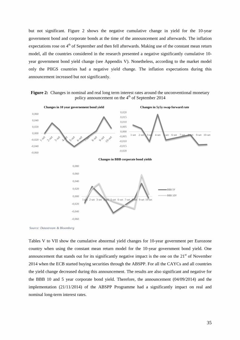
35

but not significant. Figure 2 shows the negative cumulative change in yield for the 10-year

government bond and corporate bonds at the time of the announcement and afterwards. The inflation

expectations rose on 4th of September and then fell afterwards. Making use of the constant mean return

model, all the countries considered in the research presented a negative significantly cumulative 10-

year government bond yield change (see Appendix V). Nonetheless, according to the market model

only the PIIGS countries had a negative yield change. The inflation expectations during this

announcement increased but not significantly.

Figure 2: Changes in nominal and real long term interest rates around the unconventional monetary

policy announcement on the 4th of September 2014

Tables V to VII show the cumulative abnormal yield changes for 10-year government per Eurozone

country when using the constant mean return model for the 10-year government bond yield. One

announcement that stands out for its significantly negative impact is the one on the 21st of November

2014 when the ECB started buying securities through the ABSPP. For all the CAYCs and all countries

the yield change decreased during this announcement. The results are also significant and negative for

the BBB 10 and 5 year corporate bond yield. Therefore, the announcement (04/09/2014) and the

implementation (21/11/2014) of the ABSPP Programme had a significantly impact on real and

nominal long-term interest rates.

-0,060

-0,040

-0,020

0,000

0,020

0,040

0,060

Changes in 10 year governement bond yield

-0,020

-0,015

-0,010

-0,005

0,000

0,005

0,010

0,015

0,020

1-set 2-set 3-set 4-set 5-set 6-set 7-set 8-set 9-set 10-set

Changes in 5y5y swap forward rate

-0,060

-0,040

-0,020

0,000

0,020

0,040

0,060

0,080

1-set 2-set 3-set 4-set 5-set 6-set 7-set 8-set 9-set 10-set

Changes in BBB corporate bond yields

BBB 5Y

BBB 10Y

Source: Datastream & Bloomberg

36

7. Conclusion

In this study, I found that unconventional monetary policy conducted by the ECB after the financial

crisis of 2008 had a significant effect on real and nominal long-term interest rates, which is in line

with the previous literature mentioned before. Nevertheless, whether non-standard monetary policies

are decreasing or increasing changes in nominal and real long-term interest rates around the

announcement date is uncertain.

Abnormal long-term yield changes are only decreasing on the day after an ECB announcement (t=1),

which might imply that the market is taking some time to react to the ECB unconventional monetary

policy announcements.

Regarding the overall significance of unconventional monetary policy, the results for both models (the

market model and the constant mean return) enumerated in this study are very similar. All the CAYCs,

on 10-year long-term interest rates, are significant at 1% (see tables H and I). The cumulative

abnormal yield (10-year government bond) decreased by 3.747 percentage points during CAYC [0,1],

at 1% significance level. Albeit the fact that not all the significant changes in the 10-year government

bond yield are negative (as expected).

The effect on corporate bond yields is different amongst maturities and different types of credit

ratings. A greater decline on the BBB corporate 10-year bond yield would mean that the effect of

unconventional monetary policy is being spread over corporations and households. However, the

outcome obtained indicates that BBB corporate 10-year yield changed positively around the

announcements and only CAYC [-1,1] is significant at 10%. Likewise, the BBB corporate 5-year bond

yield change increased for all CAYCs and they are significant for CAYC [-1,0] and CAYC [-1,1] at

1% level. Overall, the effect on BBB corporate 10-year bond yields is significant but the sign of the

cumulative abnormal yield change is opposite to what was expected. As predictable, the AAA

corporate 5-year bond yield followed the same pattern as the 10-year government bond yield and

declined for all CAYCs (all significant at 1%)

Against to what is aimed by the ECB, the inflation expectations decreased around the announcements

of non-standard monetary policy meaning that unconventional monetary is in fact decreasing inflation

expectations. CAYC [-1,0] and CAYC [-1,1] are significant at 1% level.

37

The fact that nominal long-term interest rates are decreasing together with expected inflation means

that the real term interest rates might decrease even further. These effects are contradictory to what has

been intended by the ECB. When using unconventional monetary policy, the main goal of the ECB is

to raise the inflation rate through investor’s inflation expectations, so that Eurozone can recover from

the actual stagnated low level of inflation and achieve their main purpose, price stability (around 2%

inflation).

Besides the overall effect of the ECB unconventional monetary policy, the yield changes behave

different depending on the type announcement itself and also on which Eurozone country is being

analysed. I found evidence of a significant cumulative abnormal negative yield change on LTROs for

all the CAYCs (on 10-year government bond yield and BBB 10-year and 5-year corporate bond

yields). However, the inflation expectations also declined significantly during those announcements.

Additionally, I found that the effect on long term interest rates can be more persistent and aligned with

the theory for a specific group of countries during some announcements. In particular, I found that the

4th of September of 2014 significantly lowered the 10-year government bond yield and BBB 5-year

bond yield for Portugal, Ireland, Italy, Greece and Spain (PIIGS).

Regarding the impact of ECB negative deposit facility rate announcements, the results are blurred. In

some of the announcements the cumulative abnormal yield changes positively, in others negatively.

However, the announcements made on 04/09/2014 and 10/03/2014 on deposit facility rate together

with another policy announcement (04/09/2014 and 10/03/2014) rose the inflation expectations at 1%

significance level.

All in all, unconventional monetary policy conducted by the ECB had a significant effect on nominal

and real long term interest rates. At this point of time it has been already 7 years after the first

unconventional monetary policy intervention. Still it remains unclear whether the long term impact of

those measures will eventually have the desired effect or if the ECB will just continue on adding more

unconventional programmes and maintain nominal interest rates negative hoping that one day they

will increase inflation to the desired 2%. If the ECB continues on maintaining these ultra-low interest

rates it might get to a point where they will be counterproductive (Hannoun, 2015). When interest

rates are very low, governments have no incentive to reduce their debt and in fact are more willing to

borrow. This implies that low rates are only hiding the problem and not fighting it. Other challenges

that might arise from low interest rates are related with banks. Should they pass the negative interest

rates on to their clients or just decrease their profits? For how long can the banks maintain? Also

insurance companies and pension funds are put at risk. For further research I would suggest not only

observing the effect on the days around the announcements but also investigate the risks that might be

consequence of prolonged low interest rates.

38

References

Acharya, V.V., Eisert, T., Eufinger, C. & Hirsch, C. W. (2015). ‘Whatever it Takes: The Real Effects

of Unconventional Monetary Policy’. IMF Conference: 16th Jacques Polak Annual Research

Conference.

Anderson, R. G., & Liu, Y. (2013). ‘How Low Can You Go? Negative Interest Rates and Investors’

Flight to Safety’. Federal Reserve Bank of St. Louis, The Regional Economist, issue January.

Assenmacher, K. & Gerlach, S. (2008). ‘The Term Structure of Interest Rates across Frequencies’.

ECB Working Paper No. 976.

Berkmen, S. P. (2012). ‘Bank of Japan’s Quantitative and Credit Easing: Are They Now More

Effective?’. IMF Working Paper No. 12/2.

Bernanke, B. S., Reinhart, V. R. & Sack, B. P., (2004).‘Monetary Policy Alternatives at the Zero

Bound: An Empirical Assessment’.FEDS Working Paper No. 2004-48.

Brand, C., Buncic, D. & Turunen, J. (2010).’ The Impact of ECB Monetary Policy Decisions and

Communication on the Yield Curve’. European Economic Review, 8 (6), 1266-1298.

Breedon, F., Chadha, J. S., & Waters, A. (2012). ‘The financial market impact of UK quantitative

easing’. Oxford Review of Economic Policy, 28 (4), 702-728.

Bowdler, C. & Radia, A. (2012). ‘Unconventional monetary policy: the assessment’. Oxford Review of

Economic Policy, 28 (4), 603–621.

Carvalho, D. & Fidora, M. (2015). ‘Capital Inflows and Euro Area Long-Term Interest Rates’. ECB

Working Paper No. 1798.

Cossetti, F. & Guidi, F. (2009). ‘ECB monetary policy and term structure of interest rates in the Euro

area: an empirical analysis’. Università Politecnica delle Marche Dipartimento di Economia.

Quaderno di ricerca n. 334.

Cox, J.C., Ingersoll, J.E. & Ross, S.A. (1985). ‘A theory of the term structure of interest rates’.

Econometrica, Vol. 53, No. 2, 385-408.

D’Amico, S. & King T. (2010). ‘Flow and stock effects of large-scale treasury Purchases’. Federal

Reserve Board Finance and Economics Discussion Series, 2010–52.

Eser, F. & Schwaab, B. (2013). ‘Assesing Asset Purchases within the ECB’s Securities Markets

Programme’. ECB Working paper series No.1587.

Falagiarda, M. & Reitz, S. (2015). ‘Announcements of ECB unconventional programs: Implications

for the sovereign spreads of stressed euro area countries’. Journal of International Money and

Finance, 53, (C), 276-295.

Fisher, I. (1930). ‘The Theory of Interest’. New York: Macmillan Co.

Gagnon, J., Raskin J.M., Remasche J. & Sack, B. (2011). ‘The financial market effects of the Federal

Reserve’s large-scale asset purchases’. International Journal of Central Banking, (7), (1), 3–

43.

http://econpapers.repec.org/article/eeejimfin/v_3a53_3ay_3a2015_3ai_3ac_3ap_3a276-295.htm

http://econpapers.repec.org/article/eeejimfin/v_3a53_3ay_3a2015_3ai_3ac_3ap_3a276-295.htm

39

Gambacorta, L., Hofmann, B. & Peersman, G. (2012). ‘The Effectiveness of Unconventional

Monetary Policy at the Zero Lower Bound: A Cross-Country Analysis’. BIS working papers,

384.

Georgoutsos, D. A. & Migiakis, P. M. (2012). ‘Benchmark Bonds Interactions Under Regime Shifts’.

European Financial Management, Vol. 18, Issue 3, 389-409.

Gerlach, S., & Lewis, J. (2010). ‘Zero lower bound, ECB interest rate policy and the financial crisis’.

De Nederlandsche Bank Working Paper No. 254.

Ghysels, E., Idier, J., Manganelli , S. & Vergote, O. (2014). ‘A High Frequency Assessment of the

ECB Securities Markets Programme’. ECB Working Paper No. 1642

Gospodinov, N. & Wei, B. (2015). ‘A Note on Extracting Inflation Expectations from Market Prices

of TIPS and Inflation Derivatives’. Federal Reserve Bank of Atlanta. Retrieved June 2, 2016

from https://www.frbatlanta.org/-/media/Documents/news/speeches/2015/note-on-extracting-

inflation-expectations.pdf.

Guidolin, M. & Thornton, D. L. (2008). ‘Predictions of Short-Term Rates and the Expectations

Hypothesis of the Term Structure of Interest Rates’. ECB Working Paper No. 977.

Hannoun, H. (2012). ‘Monetary policy in the crisis: testing the limits of monetary policy’. 47th

SEACEN Governors' Conference. Seoul, Korea, 13-14.

Hannoun, H. (2015). ‘Ultra-low or negative interest rates: what they mean for financial stability and

growth’. Bank for Interantional Settlements, Eurofi High-Level Seminar. Riga.

Honda, Y., Kuroki, Y., Tachibana, M. (2013). ‘An Injection of Base Money at Zero Interest Rates:

Empirical Evidence from the Japanese Experience 2001–2006’. Japanese Journal of Monetary and

Financial Economics, (1), 1-24.

Joyce, M., Lasaosa, A., Stevens, I. & Tong, M. (2010). ‘The Financial Market Impact of Quantitative

Easing’. Bank of England Working Paper No. 393.

Kapetanios, G., Mumtaz, H., Stevens, I. & Theodoridis, K. (2012). ‘Assesing the economy-wide

effects of quatitative easing’. The Economic Journal, 122, F316-F347.

Keister, T. (2011). 'Why Is There a “Zero Lower Bound” on Interest Rates?’. Federal Reserve Bank of

New York: Liberty Street Economics. Retrieved June 2, 2016 from

http://libertystreeteconomics.newyorkfed.org/2011/11/why-is-there-a-zero-lower-bound-on-

interest-rates.html

Koller, T., Dobbs, R., & Lund, S. (2014, Winter). ‘What effect has quantitative easing had on your

share price?’. McKinsey on Finance, 49, 15-18.

Krishnamurthy, A., & Vissing-Jorgensen, A. (2010). ‘The Effects of Quantitative Easing on Long-

term Interest Rates’. Kellogg School of Management.

Lam, W. R. (2011). ‘Bank of Japan’s Monetary Easing Measures: Are They Powerful and

Comprehensive?’. IMF Working Papers, 1-18.

40

Mackinlay, A.C. (1997). ‘Event Studies in Economics and Finance’. Journal of Economic Literature.

Vol. XXXV, 13-39.

Meaning, J., & Zhu, F. (2011). ‘The impact of recent central bank asset purchase programmes’. BIS

Quarterly Review, December 2011.

Meier, A. (2009). ‘Panacea, curse, or nonevent? Unconventional monetary policy in the United

Kingdom’. IMF Working Paper, No. 09/163, 1-47.

Mishkin, F. S. (1991). ‘Is the Fisher Effect for Real? A Reexamination of the Relationship between

Inflation and Interest Rates’. NBER Working Paper No. 3632.

Neely, J. C. (2010). ‘The Large-Scale Asset Purchases Had Large International Effects’. Federal

Reserve Bank of St.Louis, Working paper 2010-018C.

Pattipeilohy, C., van den End, J., Tabbae, M., Frost, J. & de Haan, J. (2013). ‘Unconventional

Monetary Policy of the ECB during the Financial Crisis: An Assessment and New Evidence’.

De Nederlandsche Bank Working Paper No. 381.

Randow , J. (2012). ‘Draghi May Enter Twilight Zone Where Fed Fears to Tread’. Bloomberg.

Retrieved June 2, 2016 from http://www.bloomberg.com/news/articles/2012-06-26/draghi-

may-enter-twilight-zone-where-bernanke-fears-to-tread

Rigobon, R. (2003). ‘Identification Through Heteroskedasticity’. Review of Economics and Statistics,

85, 777-92.

Rigobon, R. & Brian, S. (2003). ‘Measuring the Response of Monetary Policy to the Stock Market’.

Quarterly Journal of Economics, 118, 639-669

Rigobon, R. & Brian, S. (2004). ‘The Impact of Monetary Policy on Asset Prices’. Journal of

Monetary Economics, 51, 1553-1575

Rigobon, R. & Brian, S. (2005). ‘The Effects of War risk on US Financial Markets’. Journal of

Banking and Finance, 29, 1769-1789

Rivolta, G. (2014). ‘An Event Study Analysis of ECB Unconventional Monetary Policy’. Department

of Economics, Management and Quantitative Methods at Università degli Studi di Milano,

Working paper nr.2014-02.

Russell, S. (1992). ‘Understanding the term structure of interest rates: the expectations theory’.

Federal Reserve Bank of St. Louis Review, (74), 4

Sandler, D. & Sandler, R. (2012). ‘Multiple Event Studies in Public Finance and Labor Economics: A

Simulation Study with Applications’, Journal of Economic and Social Measurement, IOS

Press, (39), No 1-2, 31-57.

Sawson, E.T. (2011). ‘Let’s Twist Again: A High-Frequency Event-Study Analysis of Operation

Twist and Its Implications for QE2’, Federal Reserve Bank of San Francisco, Working Paper

2011-08.

Warner, J. (2015). ‘Negative interest rates put world on course for biggest mass default in history’.

The Telegraph. Retrieved June 2, 2016 from

41

http://www.telegraph.co.uk/finance/comment/jeremy-warner/11569329/Jeremy-Warner-

Negative-interest-rates-put-world-on-course-for-biggest-mass-default-in-history.html

Wright, J. H. (2012). ‘What Does Monetary Policy Do to Long‐Term Interest Rates at the Zero Lower

Bound?’. The Economic Journal, (122), Issue 564, F447-F466

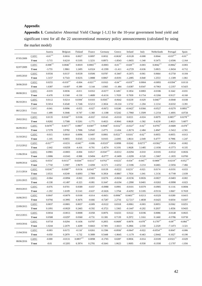
42

Appendix

Appendix I. Cumulative Abnormal Yield Change [-1,1] for the 10-year government bond yield and

significant t-test for all the 22 unconventional monetary policy announcements (calculated by using

the market model)

Austria Belgium Finland France Germany Greece Ireland Italy Netherlands Portugal Spain

07/05/2009 CAYC -0.01*** 0.0016 0.0027 0.0097 0.0032 -0.0636* -0.0128 -0.008 0.0044 -0.037*** -0.01**

T-test -3.715 0.6210 0.5195 1.3231 0.8973 -1.8543 -1.0655 -1.340 0.5475 -2.6506 -2.164

02/07/2009 CAYC -0.008*** 0.0046** 0.0019 0.0065*** -0.0003 -0.01*** -0.029*** -0.003 0.0042*** -0.0062* -0.003

T-test -3.755 1.9861 1.2495 6.0324 -0.1599 -11.411 -4.2729 -0.636 5.0815 -1.8434 -0.712

10/05/2010 CAYC 0.0556 0.0137 0.0539 0.0506 0.0787 -0.3447 -0.2075 -0.061 0.0664 -0.2750 -0.104

T-test 1.3157 0.7543 0.9235 1.0888 0.8067 -0.8191 -1.2085 -0.840 1.2553 -1.1309 -1.061

30/06/2010 CAYC 0.0255 -0.019*** -0.004 -0.021*** 0.0163 -0.04*** -0.019*** 0.0004 -0.0093 -0.0394** 0.0110

T-test 1.6387 -14.607 -0.389 -3.144 1.0365 -11.484 -3.6387 0.0347 -0.7063 -2.2357 0.5425

08/08/2011 CAYC -0.019 0.0036 -0.011 0.0352 -0.0277 0.1491* 0.1854 0.0083 -0.0186 0.1642 -0.031

T-test -0.478 0.1560 -0.150 1.4689 -0.4116 1.7020 0.7939 0.1754 -0.3266 0.9127 -8.160

06/10/2011 CAYC 0.0112 0.0214 0.0394* 0.0103 0.0505** -0.0642 0.0239 -0.029 0.0467** -0.0040 -0.038

T-test 0.5014 0.4540 1.7246 0.5213 2.3654 -10.224 1.5732 -1.204 2.1214 -0.6332 -3.391

08/12/2011 CAYC -0.041 0.0096 -0.055 -0.027 -0.0672 0.0240 -0.0425* 0.0366 -0.0527 -0.0270 0.0893***

T-test -1.499 0.3046 -0.747 -1.360 -1.1188 0.5242 -1.7960 1.3509 -1.2154 -1.4691 4.0726

29/02/2012 CAYC 0.0135 0.0160*** 0.0106 -0.033* 0.0143 -0.0310 0.0221 -0.024 0.0079 0.0857** 0.0278***

T-test 0.8282 3.7588 0.5261 -1.771 0.4023 -0.9041 0.8628 -1.582 0.4230 2.4023 5.6877

06/09/2012 CAYC 0.0478*** 0.0473*** 0.0807* 0.0387*** 0.0948** 0.0332** -0.0327* -0.02** 0.0795** -0.0689 -0.078**

T-test 2.7278 3.9782 1.7006 5.0543 2.4771 2.1434 -1.8174 -2.484 2.4947 -1.5412 -2.501

31/10/2012 CAYC -0.015 0.0010 0.0096 0.0497 0.0001 0.0521** 0.0101* -0.02** 0.0055 0.0055 -0.013

T-test -1.105 0.0855 0.6545 1.1633 0.0103 2.4395 1.8614 -2.049 0.4777 0.7996 -1.247

21/12/2012 CAYC -0.017*** -0.0231 -0.045*** -0.006 -0.0319** 0.0098 0.0242 0.0273*** -0.0362** -0.0034 -0.002

T-test -2.642 -0.8258 -4.416 -0.701 -2.4574 0.3191 1.0628 3.1485 -2.1036 -0.3773 -0.335

11/06/2014 CAYC 0.0981 -0.0003 -0.004 0.0517 -0.0347*** -0.0212 -0.0294 -0.010 -0.0105 -0.0532 0.0026

T-test 1.0086 -0.0343 -0.988 0.9494 -8.0777 -0.3499 -1.0299 -0.520 -1.5067 -1.1835 0.0700

04/09/2014 CAYC 0.0331* 0.0153*** 0.0264*** 0.0213** 0.0763*** -0.0225* -0.034** -0.045*** 0.0400*** -0.0219** -0.052***

T-test 1.7742 3.1907 2.9679 2.4284 4.1571 -1.6252 -2.3186 -3.214 4.6465 -2.5056 -7.466

21/11/2014 CAYC 0.0245** 0.0389*** 0.0156 0.0343*** 0.0139 -0.0222 0.0231* -0.021 0.0174 -0.0191 -0.033

T-test 2.0531 4.0249 0.6093 2.7984 0.3954 -0.8867 1.7054 -1.041 1.2156 -0.7749 -2.039

22/01/2015 CAYC -0.064 -0.0094 -0.063 -0.003 0.0276 -0.0634 -0.0236 0.0026 -0.0027 -0.0403 -0.002

T-test -0.338 -0.1497 -0.323 -0.081 0.1647 -0.6194 -1.2990 0.0401 -0.0263 -0.9998 -0.023

09/03/2015 CAYC -0.076 0.0701 0.0589 -0.037 -0.0988 0.0991 -0.0101 0.0379 -0.0905 0.1116 0.0694

T-test -1.202 1.6109 0.5141 -0.637 -0.5626 1.3764 -0.4292 0.5185 -0.9116 1.0667 0.7659

16/06/2015 CAYC 0.0047 -0.0079 0.0100 -0.014 -0.0651 0.0996** 0.0403*** 0.0213 -0.0329 0.0289 0.0415

T-test 0.0766 -0.3995 0.3676 -0.666 -0.7287 2.2716 12.7217 1.4838 -0.6425 0.6034 0.6507

22/09/2015 CAYC 0.0037 -0.0001 0.0037 -0.009 -0.0122 0.0318 -0.0061 -0.003 0.0053 0.0362 0.0251

T-test 0.1091 -0.0029 0.2465 -0.592 -0.3721 1.3365 -0.1447 -0.202 0.2037 1.4556 0.9435

03/12/2015 CAYC 0.0034 -0.0013 0.0008 -0.058 0.0076 0.0233 0.0122 0.0196 0.0086 -0.0148 0.0025

T-test 0.0588 -0.0297 0.0360 -0.731 0.1381 0.7139 0.2972 1.3161 0.1460 -0.5786 0.0730

10/03/2016 CAYC 0.0718 0.0294 0.1436 0.0787 0.2855 -0.0609* 0.0078 -0.078** 0.1797** -0.09*** -0.084***

T-test 1.0244 2.2679 1.4200 0.6663 0.7491 -1.6613 0.2866 -2.550 2.2320 -7.1473 -3.321

21/04/2016 CAYC -0.003 0.0172 -0.116* 0.0261 0.1596 -0.0936* -0.0647 -0.022 -0.0554*** 0.0047 -0.006

T-test -0.050 0.2870 -1.732 0.3089 0.5448 -1.8645 -1.1179 -0.463 -2.8442 0.1027 -0.190

08/06/2016 CAYC -0.000 -0.0131 0.0857*** 0.0098 -0.1765 0.0287 0.0836 -0.014 -0.0109 -0.0321** -0.029

T-test -0.01 -0.3205 6.3974 0.2781 -0.5641 1.0623 1.0695 -0.930 -0.1930 -2.1707 -1.056

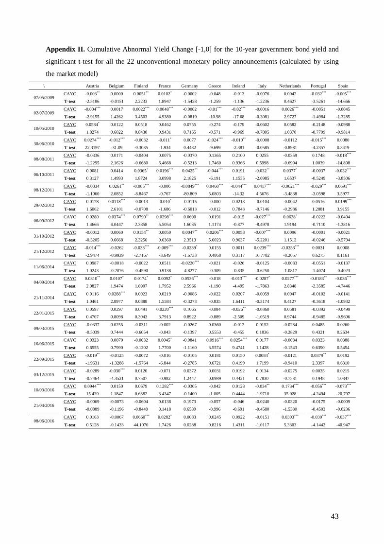
43

Appendix II. Cumulative Abnormal Yield Change [-1,0] for the 10-year government bond yield and


the market model)

\ Austria Belgium Finland France Germany Greece Ireland Italy Netherlands Portugal Spain

07/05/2009 CAYC -0.003** 0.0000 0.0051** 0.0102* -0.0002 -0.048 -0.013 -0.0076 0.0042 -0.032*** -0.005***

T-test -2.5186 -0.0151 2.2233 1.8947 -1.5428 -1.259 -1.136 -1.2236 0.4627 -3.5261 -14.666

02/07/2009 CAYC -0.004*** 0.0017 0.0022*** 0.0048*** -0.0002 -0.01*** -0.02*** -0.0016 0.0026*** -0.0051 -0.0045

T-test -2.9155 1.4262 3.4503 4.9380 -0.0819 -10.98 -17.68 -0.3081 2.9727 -1.4984 -1.3285

10/05/2010 CAYC 0.0584* 0.0122 0.0518 0.0462 0.0755 -0.274 -0.179 -0.0602 0.0582 -0.2148 -0.0988

T-test 1.8274 0.6022 0.8430 0.9431 0.7165 -0.571 -0.969 -0.7805 1.0378 -0.7799 -0.9814

30/06/2010 CAYC 0.0274*** -0.012*** -0.0032 -0.011* 0.0077 -0.024*** -0.010** -0.0008 -0.0112 -0.015*** 0.0080

T-test 22.3197 -31.09 -0.3035 -1.934 0.4432 -9.699 -2.381 -0.0585 -0.8981 -4.2357 0.3419

08/08/2011 CAYC -0.0336 0.0171 -0.0404 0.0075 -0.0370 0.1365 0.2100 0.0255 -0.0359 0.1748 -0.018***

T-test -1.2295 2.1626 -0.6680 6.4668 -0.5213 1.7460 0.9366 0.5998 -0.6994 1.0039 -14.898

06/10/2011 CAYC 0.0081 0.0414 0.0365* 0.0196*** 0.0425** -0.044*** 0.0191 -0.032** 0.0377* -0.0037 -0.032***

T-test 0.3127 1.4993 1.8724 3.0998 2.1825 -6.191 1.1535 -2.0985 1.6537 -0.5249 -3.8506

08/12/2011 CAYC -0.0334 0.0261** -0.085*** -0.006 -0.0849*** 0.0460*** -0.044*** 0.0417*** -0.0621*** -0.029*** 0.0691***

T-test -1.1060 2.0852 -8.8467 -0.767 -80.809 5.0803 -14.32 4.5676 -3.4838 -3.0598 3.5977

29/02/2012 CAYC 0.0178 0.0118*** -0.0013 -0.010* -0.0115 -0.000 0.0213 -0.0104 -0.0042 0.0516 0.0199***

T-test 1.6062 2.6101 -0.0708 -1.686 -0.6013 -0.012 0.7843 -0.7146 -0.2986 1.2881 3.9155

06/09/2012 CAYC 0.0280 0.0374*** 0.0790** 0.0298*** 0.0690 0.0191 -0.015 -0.027*** 0.0628* -0.0222 -0.0494

T-test 1.4666 4.0447 2.3858 5.5054 1.6035 1.1174 -0.877 -8.4978 1.9194 -0.7110 -1.3816

31/10/2012 CAYC -0.0012 0.0060 0.0154** 0.0050 0.0047** 0.0206*** 0.0058 -0.007*** 0.0096 -0.0001 -0.0021

T-test -0.3205 0.6668 2.3256 0.6360 2.3513 5.6023 0.9637 -5.2201 1.1512 -0.0246 -0.5794

21/12/2012 CAYC -0.014*** -0.0262 -0.033*** -0.009*** -0.0239* 0.0155 0.0011 0.0239*** -0.0353*** 0.0031 0.0008

T-test -2.9474 -0.9939 -2.7167 -3.649 -1.6733 0.4868 0.3117 16.7782 -8.2057 0.6275 0.1161

11/06/2014 CAYC 0.0987 -0.0018 -0.0022 0.0511 -0.0220*** -0.021 -0.026 -0.0125 -0.0083 -0.0551 -0.0137

T-test 1.0243 -0.2076 -0.4590 0.9138 -4.8277 -0.309 -0.835 -0.6250 -1.0817 -1.4074 -0.4023

04/09/2014 CAYC 0.0310** 0.0107* 0.0174* 0.0092* 0.0536*** -0.018 -0.013*** -0.0287* 0.0277*** -0.0183** -0.036***

T-test 2.0827 1.9474 1.6907 1.7952 2.5966 -1.190 -4.495 -1.7863 2.8348 -2.3585 -4.7446

21/11/2014 CAYC 0.0116 0.0288*** 0.0023 0.0219 -0.0086 -0.022 0.0207 -0.0059 0.0047 -0.0102 -0.0141

T-test 1.0461 2.8977 0.0888 1.5584 -0.3273 -0.835 1.6411 -0.3174 0.4127 -0.3618 -1.0932

22/01/2015 CAYC 0.0597 0.0297 0.0491 0.0220*** 0.1065 -0.084 -0.026** -0.0360 0.0581 -0.0392 -0.0499

T-test 0.4707 0.8098 0.3043 3.7913 0.8922 -0.889 -2.509 -1.0519 0.9744 -0.9485 -0.9606

09/03/2015 CAYC -0.0337 0.0255 -0.0311 -0.002 -0.0267 0.0360 -0.012 0.0152 -0.0284 0.0485 0.0260

T-test -0.5039 0.7444 -0.6054 -0.043 -0.1397 0.5553 -0.455 0.1836 -0.2829 0.4321 0.2634

16/06/2015 CAYC 0.0323 0.0070 -0.0032 0.0045* -0.0841 0.0916*** 0.0254*** 0.0177 -0.0084 0.0323 0.0388

T-test 0.6555 0.7990 -0.1202 1.7700 -1.1160 3.5574 9.4741 1.1428 -0.1543 0.6390 0.5454

22/09/2015 CAYC -0.019** -0.0125 -0.0072 -0.016 -0.0105 0.0181 0.0150 0.0084* -0.0121 0.0379** 0.0192

T-test -1.9631 -1.3288 -1.5764 -6.844 -0.2785 0.6721 0.4199 1.7199 -0.9410 2.3397 0.6310

03/12/2015 CAYC -0.0289 -0.030*** 0.0120 -0.071 0.0372 0.0031 0.0192 0.0134 -0.0275 0.0035 0.0215

T-test -0.7464 -4.3521 0.7507 -0.982 1.2447 0.0989 0.4421 0.7830 -0.7531 0.1948 1.0347

10/03/2016 CAYC 0.0944*** 0.0150 0.0679 0.1282*** -0.0305 -0.042 0.0128 -0.034** 0.1734*** -0.056*** -0.073***

T-test 15.439 1.1847 0.6382 3.4347 -0.1400 -1.005 0.4444 -1.9710 35.028 -4.2494 -20.797

21/04/2016 CAYC -0.0069 -0.0073 -0.0604 0.0138 0.1973 -0.057 -0.046 -0.0240 -0.0320 -0.0175 -0.0009

T-test -0.0889 -0.1196 -0.8449 0.1418 0.6589 -0.996 -0.691 -0.4580 -1.5380 -0.4503 -0.0236

08/06/2016 CAYC 0.0163 -0.0067 0.0660*** 0.0282* 0.0083 0.0245 0.0922 -0.0151 0.0303*** -0.030*** -0.037***

T-test 0.5128 -0.1433 44.1070 1.7426 0.0288 0.8216 1.4311 -1.0117 5.3303 -4.1442 -40.947

44

Appendix III. Cumulative Abnormal Yield Change [0,1] for the 10-year government bond yield and


the market model)


07/05/2009 CAYC -0.004*** 0.0005 -0.0009 0.0073 0.0034 -0.06** -0.0121 -0.008 0.0069 -0.0252 -0.0104*

T-test -9.3261 0.1703 -0.2528 0.8728 0.9755 -2.102 -0.9628 -1.230 1.0700 -1.5824 -1.8534

02/07/2009 CAYC -0.006*** 0.0044*** 0.0011 0.0036*** -0.0014 -0.01*** -0.022*** 0.0005 0.0025*** -0.002*** -0.0027

T-test -6.5309 2.9187 0.6423 18.905 -1.2334 -6.786 -3.4767 0.1699 3.1677 -10.798 -0.5191

10/05/2010 CAYC 0.0424 -0.0025 0.0587 0.0519 0.0936 -0.448 -0.2103 -0.07 0.0653 -0.3053* -0.1048

T-test 0.8846 -0.4616 1.0753 1.1995 1.0737 -1.463 -1.3647 -1.029 1.3343 -1.6508 -1.1054

30/06/2010 CAYC 0.0125 -0.013*** 0.0032 -0.013* 0.0211*** -0.028*** -0.011** -0.006 0.0026** -0.034** -0.0047

T-test 0.7707 -12.428 0.8106 -1.721 5.5012 -20.60 -2.0200 -0.713 1.9979 -2.1616 -0.4383

08/08/2011 CAYC -0.0157 -0.0089 -0.0209 0.0309 -0.0447 0.1200 0.1925 0.0168 -0.0263 0.1638 -0.0222***

T-test -0.3472 -0.4920 -0.2610 1.2587 -0.7077 1.2667 0.7961 0.3288 -0.4306 0.8850 -7.4088

06/10/2011 CAYC 0.0201 -0.0131 0.0309 0.0037 0.0390* -0.039*** 0.0226* -0.020 0.0393* 0.0014 -0.0268**

T-test 1.4556 -0.4870 1.2291 0.1665 1.7071 -18.28 1.7182 -0.737 1.8545 0.7047 -2.0694

08/12/2011 CAYC -0.0397* -0.0097 -0.0170 -0.021 -0.0243 0.0055 -0.0190 0.0203 -0.0305 -0.0078 0.0452***

T-test -1.6676 -0.4170 -0.2197 -0.927 -0.4074 0.1108 -0.8627 0.6669 -0.6180 -0.6644 9.6127

29/02/2012 CAYC -0.0009 0.0124*** 0.0203*** -0.031** 0.0296 -0.039* 0.0250 -0.026*** 0.0171** 0.0800*** 0.0153***

T-test -0.1218 3.1393 5.9393 -2.076 1.3460 -1.817 1.0617 -31.23 2.3724 6.8021 34.8691

06/09/2012 CAYC 0.0434*** 0.0332** 0.0578 0.0265*** 0.0818*** 0.0322*** -0.034*** -0.017 0.0645** -0.073*** -0.0713***

T-test 11.4342 2.4772 1.0624 3.0245 2.7074 8.0175 -16.384 -1.325 2.0816 -3.6725 -5.1337

31/10/2012 CAYC -0.0123 0.0025 0.0052 0.0512 -0.0033 0.0399* 0.0102*** -0.017* -0.0035 0.0033 -0.0141*

T-test -0.8278 0.1959 0.3100 1.3377 -0.5480 1.7390 5.9085 -1.906 -0.7344 0.4172 -1.6660

21/12/2012 CAYC -0.007*** 0.0032 -0.037*** 0.0001 -0.0271** 0.0180 0.0254 0.0146* -0.0164 -0.0025 0.0007

T-test -3.0974 1.0533 -4.5138 0.0080 -2.4441 0.6114 1.2199 1.8586 -1.1184 -0.2401 0.1038

11/06/2014 CAYC 0.0006 0.0050*** -0.0007 -0.002 -0.021*** 0.0239 -0.0009 0.0062*** -0.0025 -0.0060 0.0266***

T-test 0.3200 2.6047 -0.2119 -0.594 -5.3896 1.0105 -0.1480 4.6488 -1.3408 -0.6106 4.3094

04/09/2014 CAYC 0.0250 0.0127*** 0.0126** 0.0193*** 0.0598*** -0.021* -0.029** -0.039*** 0.0310*** -0.009*** -0.0374***

T-test 1.1964 3.6941 2.2870 3.8291 4.1381 -1.747 -2.2260 -6.762 4.8096 -5.2205 -6.2492

21/11/2014 CAYC 0.0242*** 0.0294*** 0.0274*** 0.0304*** 0.0313** -0.024 0.0064*** -0.027*** 0.0208*** -0.028*** -0.0320***

T-test 16.5252 3.1514 31.0264 5.4422 2.2936 -1.029 3.8325 -9.689 4.5818 -2.7492 -6.4538

22/01/2015 CAYC -0.1571* -0.0426 -0.168*** -0.011 -0.0853 0.0254* -0.0053 0.0376 -0.0616 0.0000 0.0489

T-test -1.7463 -1.1961 -2.999 -0.284 -1.1777 1.6883 -0.4994 0.9550 -1.0254 -0.0108 1.0436

09/03/2015 CAYC -0.093*** 0.0745*** 0.1001 -0.062*** -0.181*** 0.1135*** 0.0086 0.0716*** -0.1265*** 0.1435*** 0.1057***

T-test -11.633 5.0805 1.2539 -10.51 -4.9184 8.8790 1.6030 2.7406 -54.7260 8.3656 5.6211

16/06/2015 CAYC 0.0132 -0.0071 0.0247*** -0.017 0.0146 0.0667 0.0289*** 0.0048* -0.0016 -0.013** -0.0134

T-test 0.1925 -0.3106 15.8367 -0.898 0.6258 1.3172 35.7243 1.8702 -0.0334 -2.1736 -0.7111

22/09/2015 CAYC 0.0182 0.0015 0.0050 0.0002 0.0118 0.0362*** 0.0043 -0.010 0.0178 0.0254 0.0003

T-test 0.6583 0.0636 0.2991 0.0143 0.7754 4.0943 0.0918 -0.739 1.0446 0.8859 0.0253

03/12/2015 CAYC -0.0015 0.0101 0.0028 -0.059 0.0039 0.0063 0.0243 0.0214** 0.0041 -0.0074 0.0022

T-test -0.0231 0.2173 0.1106 -0.692 0.0618 0.1856 0.6353 2.3402 0.0604 -0.2552 0.0543

10/03/2016 CAYC 0.0215 0.0156 0.0565 0.0333 0.1919 -0.061** 0.0158 -0.052 0.0955 -0.068*** -0.0458**

T-test 0.3219 1.1756 0.5950 0.2515 0.4360 -2.553 0.6158 -1.478 1.1521 -41.731 -1.9636

21/04/2016 CAYC 0.0388 0.0513*** -0.121*** 0.0679 0.2107 -0.094*** -0.075** -0.036 -0.0290 -0.0060 -0.0246*

T-test 1.2217 21.5546 -11.472 1.5676 0.7366 -4.585 -1.9913 -0.900 -1.6306 -0.1188 -1.7758

08/06/2016 CAYC 0.0074 0.0138 0.0534 0.0038 -0.0367 0.0016 0.0053 -0.014 -0.0289 -0.0133 -0.0095

T-test 0.1813 0.5209 3.7948 0.0943 -0.1101 0.2276 0.2340 -0.890 -0.5401 -1.3692 -0.3603

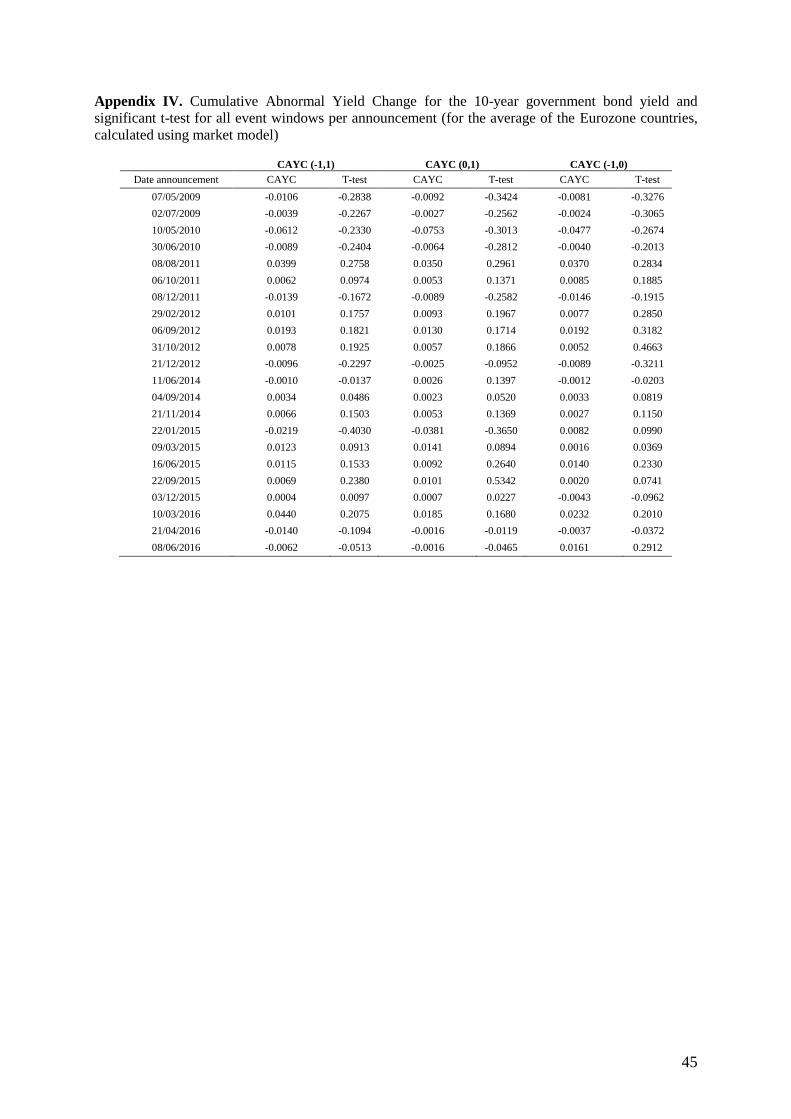
45

Appendix IV. Cumulative Abnormal Yield Change for the 10-year government bond yield and

significant t-test for all event windows per announcement (for the average of the Eurozone countries,

calculated using market model)

CAYC (-1,1) CAYC (0,1) CAYC (-1,0)

Date announcement CAYC T-test CAYC T-test CAYC T-test

07/05/2009 -0.0106 -0.2838 -0.0092 -0.3424 -0.0081 -0.3276

02/07/2009 -0.0039 -0.2267 -0.0027 -0.2562 -0.0024 -0.3065

10/05/2010 -0.0612 -0.2330 -0.0753 -0.3013 -0.0477 -0.2674

30/06/2010 -0.0089 -0.2404 -0.0064 -0.2812 -0.0040 -0.2013

08/08/2011 0.0399 0.2758 0.0350 0.2961 0.0370 0.2834

06/10/2011 0.0062 0.0974 0.0053 0.1371 0.0085 0.1885

08/12/2011 -0.0139 -0.1672 -0.0089 -0.2582 -0.0146 -0.1915

29/02/2012 0.0101 0.1757 0.0093 0.1967 0.0077 0.2850

06/09/2012 0.0193 0.1821 0.0130 0.1714 0.0192 0.3182

31/10/2012 0.0078 0.1925 0.0057 0.1866 0.0052 0.4663

21/12/2012 -0.0096 -0.2297 -0.0025 -0.0952 -0.0089 -0.3211

11/06/2014 -0.0010 -0.0137 0.0026 0.1397 -0.0012 -0.0203

04/09/2014 0.0034 0.0486 0.0023 0.0520 0.0033 0.0819

21/11/2014 0.0066 0.1503 0.0053 0.1369 0.0027 0.1150

22/01/2015 -0.0219 -0.4030 -0.0381 -0.3650 0.0082 0.0990

09/03/2015 0.0123 0.0913 0.0141 0.0894 0.0016 0.0369

16/06/2015 0.0115 0.1533 0.0092 0.2640 0.0140 0.2330

22/09/2015 0.0069 0.2380 0.0101 0.5342 0.0020 0.0741

03/12/2015 0.0004 0.0097 0.0007 0.0227 -0.0043 -0.0962

10/03/2016 0.0440 0.2075 0.0185 0.1680 0.0232 0.2010

21/04/2016 -0.0140 -0.1094 -0.0016 -0.0119 -0.0037 -0.0372

08/06/2016 -0.0062 -0.0513 -0.0016 -0.0465 0.0161 0.2912

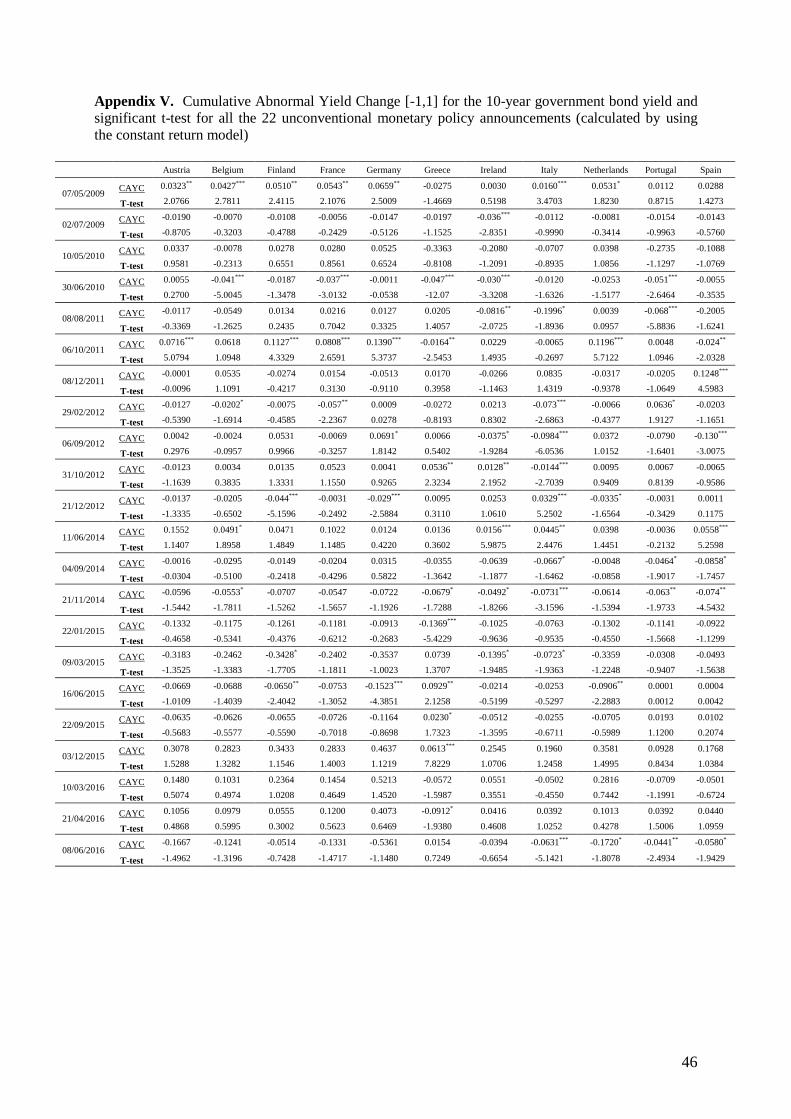
46

Appendix V. Cumulative Abnormal Yield Change [-1,1] for the 10-year government bond yield and


the constant return model)


07/05/2009 CAYC 0.0323** 0.0427*** 0.0510** 0.0543** 0.0659** -0.0275 0.0030 0.0160*** 0.0531* 0.0112 0.0288

T-test 2.0766 2.7811 2.4115 2.1076 2.5009 -1.4669 0.5198 3.4703 1.8230 0.8715 1.4273

02/07/2009 CAYC -0.0190 -0.0070 -0.0108 -0.0056 -0.0147 -0.0197 -0.036*** -0.0112 -0.0081 -0.0154 -0.0143

T-test -0.8705 -0.3203 -0.4788 -0.2429 -0.5126 -1.1525 -2.8351 -0.9990 -0.3414 -0.9963 -0.5760

10/05/2010 CAYC 0.0337 -0.0078 0.0278 0.0280 0.0525 -0.3363 -0.2080 -0.0707 0.0398 -0.2735 -0.1088

T-test 0.9581 -0.2313 0.6551 0.8561 0.6524 -0.8108 -1.2091 -0.8935 1.0856 -1.1297 -1.0769

30/06/2010 CAYC 0.0055 -0.041*** -0.0187 -0.037*** -0.0011 -0.047*** -0.030*** -0.0120 -0.0253 -0.051*** -0.0055

T-test 0.2700 -5.0045 -1.3478 -3.0132 -0.0538 -12.07 -3.3208 -1.6326 -1.5177 -2.6464 -0.3535

08/08/2011 CAYC -0.0117 -0.0549 0.0134 0.0216 0.0127 0.0205 -0.0816** -0.1996* 0.0039 -0.068*** -0.2005

T-test -0.3369 -1.2625 0.2435 0.7042 0.3325 1.4057 -2.0725 -1.8936 0.0957 -5.8836 -1.6241

06/10/2011 CAYC 0.0716*** 0.0618 0.1127*** 0.0808*** 0.1390*** -0.0164** 0.0229 -0.0065 0.1196*** 0.0048 -0.024**

T-test 5.0794 1.0948 4.3329 2.6591 5.3737 -2.5453 1.4935 -0.2697 5.7122 1.0946 -2.0328

08/12/2011 CAYC -0.0001 0.0535 -0.0274 0.0154 -0.0513 0.0170 -0.0266 0.0835 -0.0317 -0.0205 0.1248***

T-test -0.0096 1.1091 -0.4217 0.3130 -0.9110 0.3958 -1.1463 1.4319 -0.9378 -1.0649 4.5983

29/02/2012 CAYC -0.0127 -0.0202* -0.0075 -0.057** 0.0009 -0.0272 0.0213 -0.073*** -0.0066 0.0636* -0.0203

T-test -0.5390 -1.6914 -0.4585 -2.2367 0.0278 -0.8193 0.8302 -2.6863 -0.4377 1.9127 -1.1651

06/09/2012 CAYC 0.0042 -0.0024 0.0531 -0.0069 0.0691* 0.0066 -0.0375* -0.0984*** 0.0372 -0.0790 -0.130***

T-test 0.2976 -0.0957 0.9966 -0.3257 1.8142 0.5402 -1.9284 -6.0536 1.0152 -1.6401 -3.0075

31/10/2012 CAYC -0.0123 0.0034 0.0135 0.0523 0.0041 0.0536** 0.0128** -0.0144*** 0.0095 0.0067 -0.0065

T-test -1.1639 0.3835 1.3331 1.1550 0.9265 2.3234 2.1952 -2.7039 0.9409 0.8139 -0.9586

21/12/2012 CAYC -0.0137 -0.0205 -0.044*** -0.0031 -0.029*** 0.0095 0.0253 0.0329*** -0.0335* -0.0031 0.0011

T-test -1.3335 -0.6502 -5.1596 -0.2492 -2.5884 0.3110 1.0610 5.2502 -1.6564 -0.3429 0.1175

11/06/2014 CAYC 0.1552 0.0491* 0.0471 0.1022 0.0124 0.0136 0.0156*** 0.0445** 0.0398 -0.0036 0.0558***

T-test 1.1407 1.8958 1.4849 1.1485 0.4220 0.3602 5.9875 2.4476 1.4451 -0.2132 5.2598

04/09/2014 CAYC -0.0016 -0.0295 -0.0149 -0.0204 0.0315 -0.0355 -0.0639 -0.0667* -0.0048 -0.0464* -0.0858*

T-test -0.0304 -0.5100 -0.2418 -0.4296 0.5822 -1.3642 -1.1877 -1.6462 -0.0858 -1.9017 -1.7457

21/11/2014 CAYC -0.0596 -0.0553* -0.0707 -0.0547 -0.0722 -0.0679* -0.0492* -0.0731*** -0.0614 -0.063** -0.074**

T-test -1.5442 -1.7811 -1.5262 -1.5657 -1.1926 -1.7288 -1.8266 -3.1596 -1.5394 -1.9733 -4.5432

22/01/2015 CAYC -0.1332 -0.1175 -0.1261 -0.1181 -0.0913 -0.1369*** -0.1025 -0.0763 -0.1302 -0.1141 -0.0922

T-test -0.4658 -0.5341 -0.4376 -0.6212 -0.2683 -5.4229 -0.9636 -0.9535 -0.4550 -1.5668 -1.1299

09/03/2015 CAYC -0.3183 -0.2462 -0.3428* -0.2402 -0.3537 0.0739 -0.1395* -0.0723* -0.3359 -0.0308 -0.0493

T-test -1.3525 -1.3383 -1.7705 -1.1811 -1.0023 1.3707 -1.9485 -1.9363 -1.2248 -0.9407 -1.5638

16/06/2015 CAYC -0.0669 -0.0688 -0.0650** -0.0753 -0.1523*** 0.0929** -0.0214 -0.0253 -0.0906** 0.0001 0.0004

T-test -1.0109 -1.4039 -2.4042 -1.3052 -4.3851 2.1258 -0.5199 -0.5297 -2.2883 0.0012 0.0042

22/09/2015 CAYC -0.0635 -0.0626 -0.0655 -0.0726 -0.1164 0.0230* -0.0512 -0.0255 -0.0705 0.0193 0.0102

T-test -0.5683 -0.5577 -0.5590 -0.7018 -0.8698 1.7323 -1.3595 -0.6711 -0.5989 1.1200 0.2074

03/12/2015 CAYC 0.3078 0.2823 0.3433 0.2833 0.4637 0.0613*** 0.2545 0.1960 0.3581 0.0928 0.1768

T-test 1.5288 1.3282 1.1546 1.4003 1.1219 7.8229 1.0706 1.2458 1.4995 0.8434 1.0384

10/03/2016 CAYC 0.1480 0.1031 0.2364 0.1454 0.5213 -0.0572 0.0551 -0.0502 0.2816 -0.0709 -0.0501

T-test 0.5074 0.4974 1.0208 0.4649 1.4520 -1.5987 0.3551 -0.4550 0.7442 -1.1991 -0.6724

21/04/2016 CAYC 0.1056 0.0979 0.0555 0.1200 0.4073 -0.0912* 0.0416 0.0392 0.1013 0.0392 0.0440

T-test 0.4868 0.5995 0.3002 0.5623 0.6469 -1.9380 0.4608 1.0252 0.4278 1.5006 1.0959

08/06/2016 CAYC -0.1667 -0.1241 -0.0514 -0.1331 -0.5361 0.0154 -0.0394 -0.0631*** -0.1720* -0.0441** -0.0580*

T-test -1.4962 -1.3196 -0.7428 -1.4717 -1.1480 0.7249 -0.6654 -5.1421 -1.8078 -2.4934 -1.9429

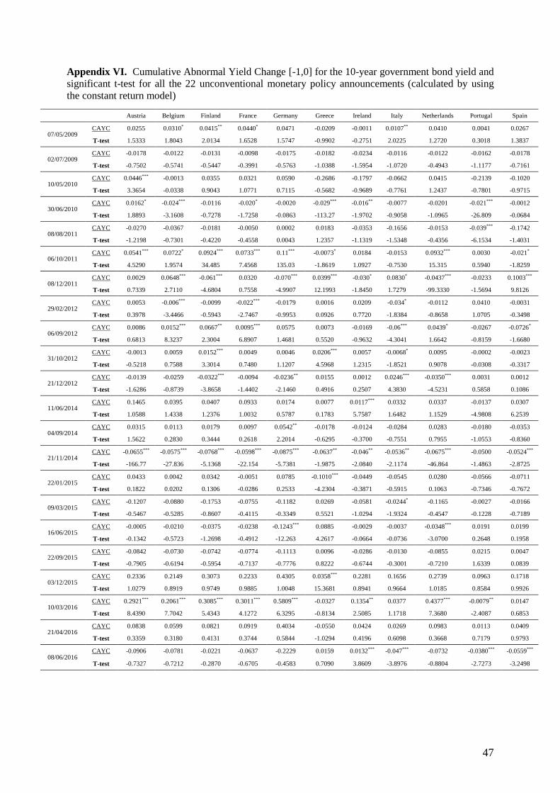
47

Appendix VI. Cumulative Abnormal Yield Change [-1,0] for the 10-year government bond yield and




07/05/2009 CAYC 0.0255 0.0310* 0.0415** 0.0440* 0.0471 -0.0209 -0.0011 0.0107** 0.0410 0.0041 0.0267

T-test 1.5333 1.8043 2.0134 1.6528 1.5747 -0.9902 -0.2751 2.0225 1.2720 0.3018 1.3837

02/07/2009 CAYC -0.0178 -0.0122 -0.0131 -0.0098 -0.0175 -0.0182 -0.0234 -0.0116 -0.0122 -0.0162 -0.0178

T-test -0.7502 -0.5741 -0.5447 -0.3991 -0.5763 -1.0388 -1.5954 -1.0720 -0.4943 -1.1177 -0.7161

10/05/2010 CAYC 0.0446*** -0.0013 0.0355 0.0321 0.0590 -0.2686 -0.1797 -0.0662 0.0415 -0.2139 -0.1020

T-test 3.3654 -0.0338 0.9043 1.0771 0.7115 -0.5682 -0.9689 -0.7761 1.2437 -0.7801 -0.9715

30/06/2010 CAYC 0.0162* -0.024*** -0.0116 -0.020* -0.0020 -0.029*** -0.016** -0.0077 -0.0201 -0.021*** -0.0012

T-test 1.8893 -3.1608 -0.7278 -1.7258 -0.0863 -113.27 -1.9702 -0.9058 -1.0965 -26.809 -0.0684

08/08/2011 CAYC -0.0270 -0.0367 -0.0181 -0.0050 0.0002 0.0183 -0.0353 -0.1656 -0.0153 -0.039*** -0.1742

T-test -1.2198 -0.7301 -0.4220 -0.4558 0.0043 1.2357 -1.1319 -1.5348 -0.4356 -6.1534 -1.4031

06/10/2011 CAYC 0.0541*** 0.0722* 0.0924*** 0.0733*** 0.11*** -0.0073* 0.0184 -0.0153 0.0932*** 0.0030 -0.021*

T-test 4.5290 1.9574 34.485 7.4568 135.03 -1.8619 1.0927 -0.7530 15.315 0.5940 -1.8259

08/12/2011 CAYC 0.0029 0.0648*** -0.061*** 0.0320 -0.070*** 0.0399*** -0.030* 0.0830* -0.0437*** -0.0233 0.1003***

T-test 0.7339 2.7110 -4.6804 0.7558 -4.9907 12.1993 -1.8450 1.7279 -99.3330 -1.5694 9.8126

29/02/2012 CAYC 0.0053 -0.006*** -0.0099 -0.022*** -0.0179 0.0016 0.0209 -0.034* -0.0112 0.0410 -0.0031

T-test 0.3978 -3.4466 -0.5943 -2.7467 -0.9953 0.0926 0.7720 -1.8384 -0.8658 1.0705 -0.3498

06/09/2012 CAYC 0.0086 0.0152*** 0.0667** 0.0095*** 0.0575 0.0073 -0.0169 -0.06*** 0.0439* -0.0267 -0.0726*

T-test 0.6813 8.3237 2.3004 6.8907 1.4681 0.5520 -0.9632 -4.3041 1.6642 -0.8159 -1.6680

31/10/2012 CAYC -0.0013 0.0059 0.0152*** 0.0049 0.0046 0.0206*** 0.0057 -0.0068* 0.0095 -0.0002 -0.0023

T-test -0.5218 0.7588 3.3014 0.7480 1.1207 4.5968 1.2315 -1.8521 0.9078 -0.0308 -0.3317

21/12/2012 CAYC -0.0139 -0.0259 -0.0322*** -0.0094 -0.0236** 0.0155 0.0012 0.0246*** -0.0350*** 0.0031 0.0012

T-test -1.6286 -0.8739 -3.8658 -1.4402 -2.1460 0.4916 0.2507 4.3830 -4.5231 0.5858 0.1086

11/06/2014 CAYC 0.1465 0.0395 0.0407 0.0933 0.0174 0.0077 0.0117*** 0.0332 0.0337 -0.0137 0.0307

T-test 1.0588 1.4338 1.2376 1.0032 0.5787 0.1783 5.7587 1.6482 1.1529 -4.9808 6.2539

04/09/2014 CAYC 0.0315 0.0113 0.0179 0.0097 0.0542** -0.0178 -0.0124 -0.0284 0.0283 -0.0180 -0.0353

T-test 1.5622 0.2830 0.3444 0.2618 2.2014 -0.6295 -0.3700 -0.7551 0.7955 -1.0553 -0.8360

21/11/2014 CAYC -0.0655*** -0.0575*** -0.0768*** -0.0598*** -0.0875*** -0.0637** -0.046** -0.0536** -0.0675*** -0.0500 -0.0524***

T-test -166.77 -27.836 -5.1368 -22.154 -5.7381 -1.9875 -2.0840 -2.1174 -46.864 -1.4863 -2.8725

22/01/2015 CAYC 0.0433 0.0042 0.0342 -0.0051 0.0785 -0.1010*** -0.0449 -0.0545 0.0280 -0.0566 -0.0711

T-test 0.1822 0.0202 0.1306 -0.0286 0.2533 -4.2304 -0.3871 -0.5915 0.1063 -0.7346 -0.7672

09/03/2015 CAYC -0.1207 -0.0880 -0.1753 -0.0755 -0.1182 0.0269 -0.0581 -0.0244* -0.1165 -0.0027 -0.0166

T-test -0.5467 -0.5285 -0.8607 -0.4115 -0.3349 0.5521 -1.0294 -1.9324 -0.4547 -0.1228 -0.7189

16/06/2015 CAYC -0.0005 -0.0210 -0.0375 -0.0238 -0.1243*** 0.0885 -0.0029 -0.0037 -0.0348*** 0.0191 0.0199

T-test -0.1342 -0.5723 -1.2698 -0.4912 -12.263 4.2617 -0.0664 -0.0736 -3.0700 0.2648 0.1958

22/09/2015 CAYC -0.0842 -0.0730 -0.0742 -0.0774 -0.1113 0.0096 -0.0286 -0.0130 -0.0855 0.0215 0.0047

T-test -0.7905 -0.6194 -0.5954 -0.7137 -0.7776 0.8222 -0.6744 -0.3001 -0.7210 1.6339 0.0839

03/12/2015 CAYC 0.2336 0.2149 0.3073 0.2233 0.4305 0.0358*** 0.2281 0.1656 0.2739 0.0963 0.1718

T-test 1.0279 0.8919 0.9749 0.9885 1.0048 15.3681 0.8941 0.9664 1.0185 0.8584 0.9926

10/03/2016 CAYC 0.2921*** 0.2061*** 0.3085*** 0.3011*** 0.5809*** -0.0327 0.1354** 0.0377 0.4377*** -0.0079** 0.0147

T-test 8.4390 7.7042 5.4343 4.1272 6.3295 -0.8134 2.5085 1.1718 7.3680 -2.4087 0.6853

21/04/2016 CAYC 0.0838 0.0599 0.0821 0.0919 0.4034 -0.0550 0.0424 0.0269 0.0983 0.0113 0.0409

T-test 0.3359 0.3180 0.4131 0.3744 0.5844 -1.0294 0.4196 0.6098 0.3668 0.7179 0.9793

08/06/2016 CAYC -0.0906 -0.0781 -0.0221 -0.0637 -0.2229 0.0159 0.0132*** -0.047*** -0.0732 -0.0380*** -0.0559***

T-test -0.7327 -0.7212 -0.2870 -0.6705 -0.4583 0.7090 3.8609 -3.8976 -0.8804 -2.7273 -3.2498

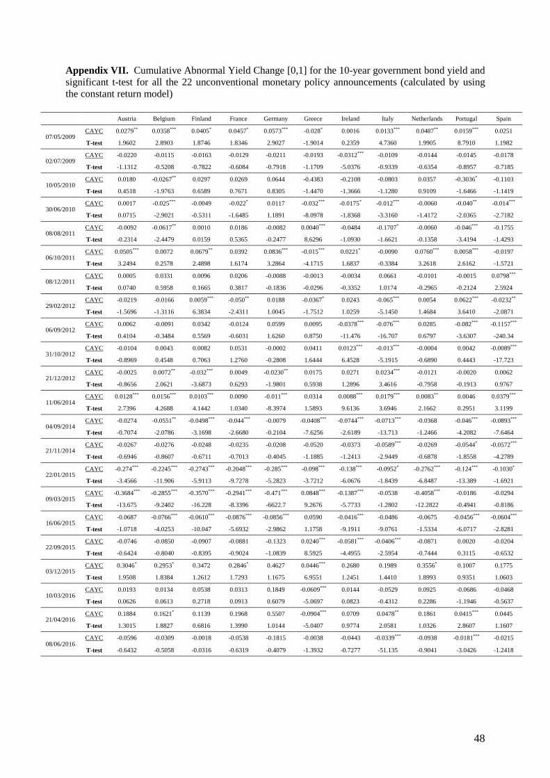
48

Appendix VII. Cumulative Abnormal Yield Change [0,1] for the 10-year government bond yield and




07/05/2009 CAYC 0.0279** 0.0358*** 0.0405* 0.0457* 0.0573*** -0.028* 0.0016 0.0133*** 0.0487** 0.0159*** 0.0251

T-test 1.9602 2.8903 1.8746 1.8346 2.9027 -1.9014 0.2359 4.7360 1.9905 8.7910 1.1982

02/07/2009 CAYC -0.0220 -0.0115 -0.0163 -0.0129 -0.0211 -0.0193 -0.0312*** -0.0109 -0.0144 -0.0145 -0.0178

T-test -1.1312 -0.5208 -0.7822 -0.6084 -0.7918 -1.1709 -5.0376 -0.9339 -0.6354 -0.8957 -0.7185

10/05/2010 CAYC 0.0180 -0.0267** 0.0297 0.0269 0.0644 -0.4383 -0.2108 -0.0803 0.0357 -0.3036* -0.1103

T-test 0.4518 -1.9763 0.6589 0.7671 0.8305 -1.4470 -1.3666 -1.1280 0.9109 -1.6466 -1.1419

30/06/2010 CAYC 0.0017 -0.025*** -0.0049 -0.022* 0.0117 -0.032*** -0.0175* -0.012*** -0.0060 -0.040** -0.014***

T-test 0.0715 -2.9021 -0.5311 -1.6485 1.1891 -8.0978 -1.8368 -3.3160 -1.4172 -2.0365 -2.7182

08/08/2011 CAYC -0.0092 -0.0617** 0.0010 0.0186 -0.0082 0.0040*** -0.0484 -0.1707* -0.0060 -0.046*** -0.1755

T-test -0.2314 -2.4479 0.0159 0.5365 -0.2477 8.6296 -1.0930 -1.6621 -0.1358 -3.4194 -1.4293

06/10/2011 CAYC 0.0505*** 0.0072 0.0679** 0.0392 0.0836*** -0.015*** 0.0221* -0.0090 0.0760*** 0.0058*** -0.0197

T-test 3.2494 0.2578 2.4898 1.6174 3.2864 -4.1715 1.6837 -0.3384 3.2618 2.6162 -1.5721

08/12/2011 CAYC 0.0005 0.0331 0.0096 0.0206 -0.0088 -0.0013 -0.0034 0.0661 -0.0101 -0.0015 0.0798***

T-test 0.0740 0.5958 0.1665 0.3817 -0.1836 -0.0296 -0.3352 1.0174 -0.2965 -0.2124 2.5924

29/02/2012 CAYC -0.0219 -0.0166 0.0059*** -0.050** 0.0188 -0.0367* 0.0243 -0.065*** 0.0054 0.0622*** -0.0232**

T-test -1.5696 -1.3116 6.3834 -2.4311 1.0045 -1.7512 1.0259 -5.1450 1.4684 3.6410 -2.0871

06/09/2012 CAYC 0.0062 -0.0091 0.0342 -0.0124 0.0599 0.0095 -0.0378*** -0.076*** 0.0285 -0.082*** -0.1157***

T-test 0.4104 -0.3484 0.5569 -0.6031 1.6260 0.8750 -11.476 -16.707 0.6797 -3.6307 -240.34

31/10/2012 CAYC -0.0104 0.0043 0.0082 0.0531 -0.0002 0.0411 0.0123*** -0.013*** -0.0004 0.0042 -0.0089***

T-test -0.8969 0.4548 0.7063 1.2760 -0.2808 1.6444 6.4528 -5.1915 -0.6890 0.4443 -17.723

21/12/2012 CAYC -0.0025 0.0072** -0.032*** 0.0049 -0.0230** 0.0175 0.0271 0.0234*** -0.0121 -0.0020 0.0062

T-test -0.8656 2.0621 -3.6873 0.6293 -1.9801 0.5938 1.2896 3.4616 -0.7958 -0.1913 0.9767

11/06/2014 CAYC 0.0128*** 0.0156*** 0.0103*** 0.0090 -0.011*** 0.0314 0.0088*** 0.0179*** 0.0083** 0.0046 0.0379***

T-test 2.7396 4.2688 4.1442 1.0340 -8.3974 1.5893 9.6136 3.6946 2.1662 0.2951 3.1199

04/09/2014 CAYC -0.0274 -0.0551** -0.0498*** -0.044*** -0.0079 -0.0408*** -0.0744*** -0.0713*** -0.0368 -0.046*** -0.0893***

T-test -0.7074 -2.0786 -3.1698 -2.6680 -0.2104 -7.6256 -2.6189 -13.713 -1.2466 -4.2082 -7.6464

21/11/2014 CAYC -0.0267 -0.0276 -0.0248 -0.0235 -0.0208 -0.0520 -0.0373 -0.0589*** -0.0269 -0.0544* -0.0572***

T-test -0.6946 -0.8607 -0.6711 -0.7013 -0.4045 -1.1885 -1.2413 -2.9449 -0.6878 -1.8558 -4.2789

22/01/2015 CAYC -0.274*** -0.2245*** -0.2743*** -0.2048*** -0.285*** -0.098*** -0.138*** -0.0952* -0.2762*** -0.124*** -0.1030*

T-test -3.4566 -11.906 -5.9113 -9.7278 -5.2823 -3.7212 -6.0676 -1.8439 -6.8487 -13.389 -1.6921

09/03/2015 CAYC -0.3684*** -0.2855*** -0.3570*** -0.2941*** -0.471*** 0.0848*** -0.1387*** -0.0538 -0.4058*** -0.0186 -0.0294

T-test -13.675 -9.2402 -16.228 -8.3396 -6622.7 9.2676 -5.7733 -1.2802 -12.2822 -0.4941 -0.8186

16/06/2015 CAYC -0.0687 -0.0766*** -0.0610*** -0.0876*** -0.0856*** 0.0590 -0.0416*** -0.0486 -0.0675 -0.0456*** -0.0604***

T-test -1.0718 -4.0253 -10.047 -5.6932 -2.9862 1.1758 -9.1911 -9.0761 -1.5334 -6.0717 -2.8281

22/09/2015 CAYC -0.0746 -0.0850 -0.0907 -0.0881 -0.1323 0.0240*** -0.0581*** -0.0406*** -0.0871 0.0020 -0.0204

T-test -0.6424 -0.8040 -0.8395 -0.9024 -1.0839 8.5925 -4.4955 -2.5954 -0.7444 0.3115 -0.6532

03/12/2015 CAYC 0.3046* 0.2953* 0.3472 0.2846* 0.4627 0.0446*** 0.2680 0.1989 0.3556* 0.1007 0.1775

T-test 1.9508 1.8384 1.2612 1.7293 1.1675 6.9551 1.2451 1.4410 1.8993 0.9351 1.0603

10/03/2016 CAYC 0.0193 0.0134 0.0538 0.0313 0.1849 -0.0609*** 0.0144 -0.0529 0.0925 -0.0686 -0.0468

T-test 0.0626 0.0613 0.2718 0.0913 0.6079 -5.0697 0.0823 -0.4312 0.2286 -1.1946 -0.5637

21/04/2016 CAYC 0.1884 0.1621* 0.1139 0.1968 0.5507 -0.0904*** 0.0709 0.0478** 0.1861 0.0415*** 0.0445

T-test 1.3015 1.8827 0.6816 1.3990 1.0144 -5.0407 0.9774 2.0581 1.0326 2.8607 1.1607

08/06/2016 CAYC -0.0596 -0.0309 -0.0018 -0.0538 -0.1815 -0.0038 -0.0443 -0.0339*** -0.0938 -0.0181*** -0.0215

T-test -0.6432 -0.5058 -0.0316 -0.6319 -0.4079 -1.3932 -0.7277 -51.135 -0.9041 -3.0426 -1.2418

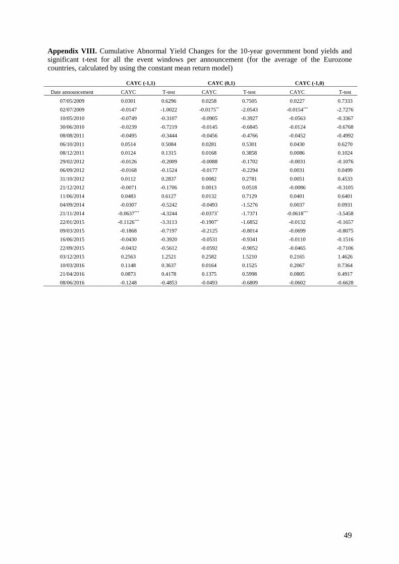
49

Appendix VIII. Cumulative Abnormal Yield Changes for the 10-year government bond yields and

significant t-test for all the event windows per announcement (for the average of the Eurozone

countries, calculated by using the constant mean return model)

CAYC (-1,1) CAYC (0,1) CAYC (-1,0)


07/05/2009 0.0301 0.6296 0.0258 0.7505 0.0227 0.7333

02/07/2009 -0.0147 -1.0022 -0.0175** -2.0543 -0.0154*** -2.7276

10/05/2010 -0.0749 -0.3107 -0.0905 -0.3927 -0.0563 -0.3367

30/06/2010 -0.0239 -0.7219 -0.0145 -0.6845 -0.0124 -0.6768

08/08/2011 -0.0495 -0.3444 -0.0456 -0.4766 -0.0452 -0.4992

06/10/2011 0.0514 0.5084 0.0281 0.5301 0.0430 0.6270

08/12/2011 0.0124 0.1315 0.0168 0.3858 0.0086 0.1024

29/02/2012 -0.0126 -0.2009 -0.0088 -0.1702 -0.0031 -0.1076

06/09/2012 -0.0168 -0.1524 -0.0177 -0.2294 0.0031 0.0499

31/10/2012 0.0112 0.2837 0.0082 0.2781 0.0051 0.4533

21/12/2012 -0.0071 -0.1706 0.0013 0.0518 -0.0086 -0.3105

11/06/2014 0.0483 0.6127 0.0132 0.7129 0.0401 0.6401

04/09/2014 -0.0307 -0.5242 -0.0493 -1.5276 0.0037 0.0931

21/11/2014 -0.0637*** -4.3244 -0.0373* -1.7371 -0.0618*** -3.5458

22/01/2015 -0.1126*** -3.3113 -0.1907* -1.6852 -0.0132 -0.1657

09/03/2015 -0.1868 -0.7197 -0.2125 -0.8014 -0.0699 -0.8075

16/06/2015 -0.0430 -0.3920 -0.0531 -0.9341 -0.0110 -0.1516

22/09/2015 -0.0432 -0.5612 -0.0592 -0.9052 -0.0465 -0.7106

03/12/2015 0.2563 1.2521 0.2582 1.5210 0.2165 1.4626

10/03/2016 0.1148 0.3637 0.0164 0.1525 0.2067 0.7364

21/04/2016 0.0873 0.4178 0.1375 0.5998 0.0805 0.4917

08/06/2016 -0.1248 -0.4853 -0.0493 -0.6809 -0.0602 -0.6628

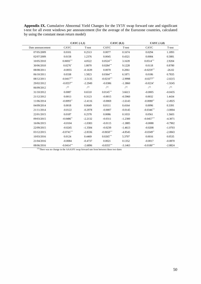
50

Appendix IX. Cumulative Abnormal Yield Changes for the 5Y5Y swap forward rate and significant

t-test for all event windows per announcement (for the average of the Eurozone countries, calculated

by using the constant mean return model)

CAYC (-1,1) CAYC (0,1) CAYC (-1,0)


07/05/2009 0.0101 0.2513 0.0077 0.1674 0.0294 1.1893

02/07/2009 0.0158 1.2376 0.0045 0.4321 0.0084 0.5881

10/05/2010 0.0693*** 4.0522 0.0524*** 3.1639 0.0514*** 2.9204

30/06/2010 0.0276* 1.8070 0.0284*** 9.1228 0.0118 0.8780

08/08/2011 -0.0055 -0.1639 0.0070 0.2061 -0.0259*** -26.02

06/10/2011 0.0338 1.5823 0.0364*** 6.1871 0.0186 0.7835

08/12/2011 -0.0417*** -3.5135 -0.0210*** -2.9998 -0.0277** -2.0215

29/02/2012 -0.0557** -2.2949 -0.0386 -1.3860 -0.0224* -1.9245

06/09/2012 -(1) -(1) -(1) -(1) -(1) -(1)

31/10/2012 0.0087 0.6510 0.0145*** 3.6613 -0.0005 -0.0435

21/12/2012 0.0013 0.3123 -0.0015 -0.5960 0.0032 1.4434

11/06/2014 -0.0093** -2.4116 -0.0069 -1.6143 -0.0080** -2.4925

04/09/2014 0.0018 0.0649 0.0111 0.4164 0.0096 0.3391

21/11/2014 -0.0122 -0.2978 -0.0007 -0.0145 -0.0346*** -3.0004

22/01/2015 0.0187 0.2578 0.0086 0.1033 0.0561 1.5603

09/03/2015 -0.0486** -2.2132 -0.0311 -1.2300 -0.0457*** -4.3071

16/06/2015 -0.0104 -1.0383 -0.0115 -1.3885 -0.0088 -0.7902

22/09/2015 -0.0245 -1.3584 -0.0239 -1.4613 -0.0208 -1.0703

03/12/2015 -0.0741*** -2.8336 -0.0650*** -4.8545 -0.0349** -2.0843

10/03/2016 0.0124 0.4469 0.0265*** 5.3707 0.0016 0.0535

21/04/2016 -0.0084 -0.4737 0.0021 0.1352 -0.0017 -0.0870

08/06/2016 -0.0414*** -2.6896 -0.0355*** -3.1463 -0.0180*** -2.8824 (1)

There was no change in the AAA10Y swap forward rate from between these two dates

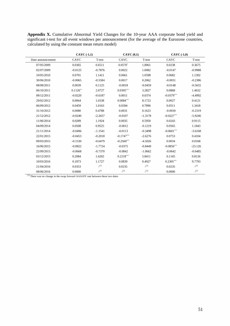
51

Appendix X. Cumulative Abnormal Yield Changes for the 10-year AAA corporate bond yield and


calculated by using the constant mean return model)

CAYC (-1,1) CAYC (0,1) CAYC (-1,0)


07/05/2009 0.0365 0.6511 0.0570* 1.8061 0.0238 0.3675

02/07/2009 -0.0125 -0.7876 0.0022 1.0082 -0.0147 -0.9988

10/05/2010 0.0701 1.1411 0.0661 1.0598 0.0682 1.1302

30/06/2010 -0.0065 -0.5584 0.0017 0.2062 -0.0031 -0.2386

08/08/2011 0.0039 0.1125 -0.0018 -0.0459 -0.0148 -0.5655

06/10/2011 0.1126** 2.0727 0.0395*** 3.2827 0.0868 1.4632

08/12/2011 -0.0220 -0.6187 0.0011 0.0374 -0.0379*** -4.4992

29/02/2012 0.0064 1.0338 0.0084*** 8.1723 0.0027 0.4121

06/09/2012 0.0459 1.0163 0.0394 0.7896 0.0511 1.3418

31/10/2012 0.0080 0.4788 0.0031 0.1623 -0.0030 -0.2319

21/12/2012 -0.0240 -2.2657 -0.0107 -1.3178 -0.0227*** -5.9246

11/06/2014 0.0289 1.1924 0.0035 0.5950 0.0243 0.9115

04/09/2014 0.0508 0.9525 -0.0012 -0.1219 0.0565 1.1843

21/11/2014 -0.0496 -1.1541 -0.0113 -0.3498 -0.0601*** -3.6168

22/01/2015 -0.0453 -0.2018 -0.1747*** -2.6276 0.0753 0.4104

09/03/2015 -0.1530 -0.6479 -0.2560*** -4.5026 0.0034 0.0168

16/06/2015 -0.0822 -1.7724 -0.0375 -0.8449 -0.0856*** -23.126

22/09/2015 -0.0668 -0.7370 -0.0842 -1.0662 -0.0642 -0.6485

03/12/2015 0.2084 1.6202 0.2218*** 5.8411 0.1165 0.8126

10/03/2016 0.1873 1.1727 0.0839 0.4927 0.2305*** 9.7793

21/04/2016 0.0353 -(1) 0.0235 -(1) 0.0235 -(1)

08/06/2016 0.0000 -(1) -(1) -(1) 0.0000 -(1) (1)

There was no change in the swap forward AAA10Y rate between these two dates

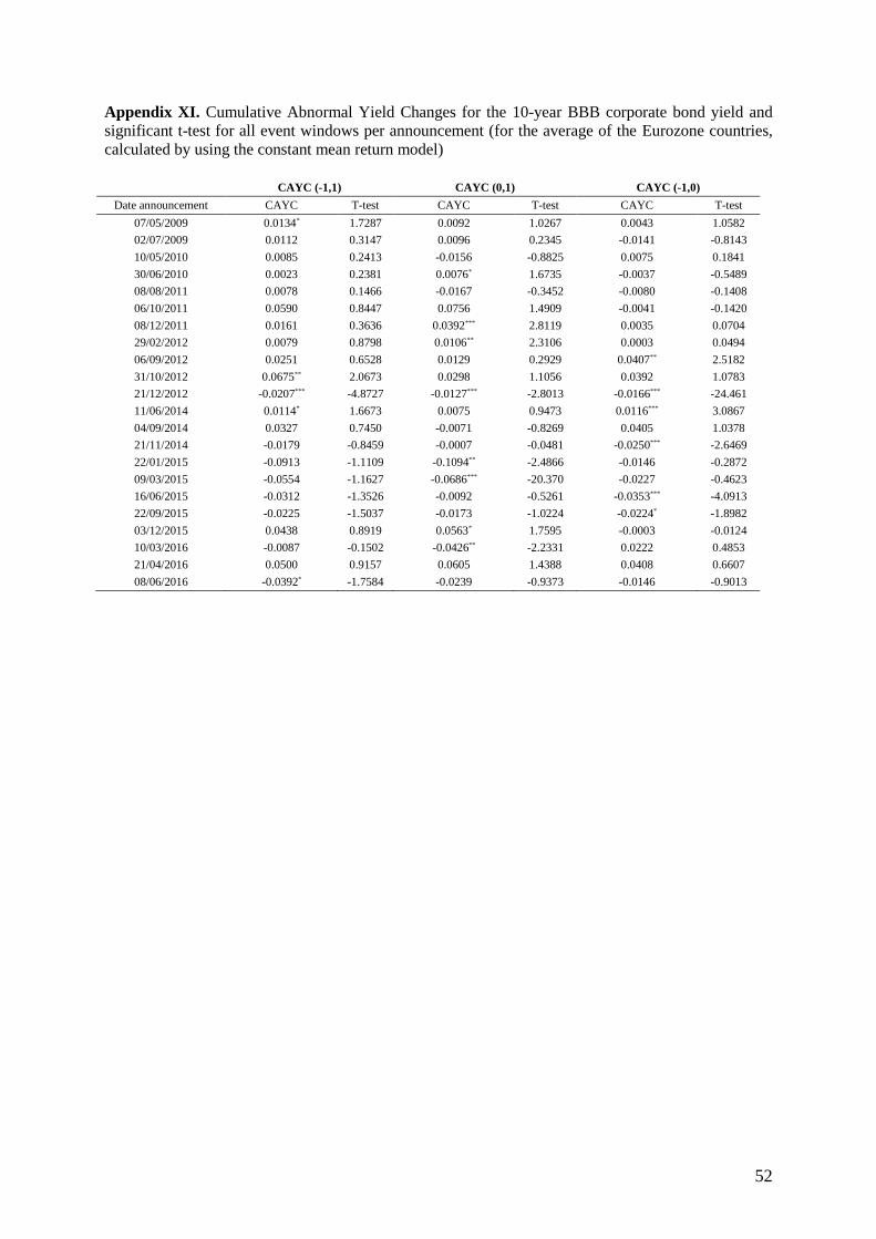
52

Appendix XI. Cumulative Abnormal Yield Changes for the 10-year BBB corporate bond yield and



CAYC (-1,1) CAYC (0,1) CAYC (-1,0)


07/05/2009 0.0134* 1.7287 0.0092 1.0267 0.0043 1.0582

02/07/2009 0.0112 0.3147 0.0096 0.2345 -0.0141 -0.8143

10/05/2010 0.0085 0.2413 -0.0156 -0.8825 0.0075 0.1841

30/06/2010 0.0023 0.2381 0.0076* 1.6735 -0.0037 -0.5489

08/08/2011 0.0078 0.1466 -0.0167 -0.3452 -0.0080 -0.1408

06/10/2011 0.0590 0.8447 0.0756 1.4909 -0.0041 -0.1420

08/12/2011 0.0161 0.3636 0.0392*** 2.8119 0.0035 0.0704

29/02/2012 0.0079 0.8798 0.0106** 2.3106 0.0003 0.0494

06/09/2012 0.0251 0.6528 0.0129 0.2929 0.0407** 2.5182

31/10/2012 0.0675** 2.0673 0.0298 1.1056 0.0392 1.0783

21/12/2012 -0.0207*** -4.8727 -0.0127*** -2.8013 -0.0166*** -24.461

11/06/2014 0.0114* 1.6673 0.0075 0.9473 0.0116*** 3.0867

04/09/2014 0.0327 0.7450 -0.0071 -0.8269 0.0405 1.0378

21/11/2014 -0.0179 -0.8459 -0.0007 -0.0481 -0.0250*** -2.6469

22/01/2015 -0.0913 -1.1109 -0.1094** -2.4866 -0.0146 -0.2872

09/03/2015 -0.0554 -1.1627 -0.0686*** -20.370 -0.0227 -0.4623

16/06/2015 -0.0312 -1.3526 -0.0092 -0.5261 -0.0353*** -4.0913

22/09/2015 -0.0225 -1.5037 -0.0173 -1.0224 -0.0224* -1.8982

03/12/2015 0.0438 0.8919 0.0563* 1.7595 -0.0003 -0.0124

10/03/2016 -0.0087 -0.1502 -0.0426** -2.2331 0.0222 0.4853

21/04/2016 0.0500 0.9157 0.0605 1.4388 0.0408 0.6607

08/06/2016 -0.0392* -1.7584 -0.0239 -0.9373 -0.0146 -0.9013

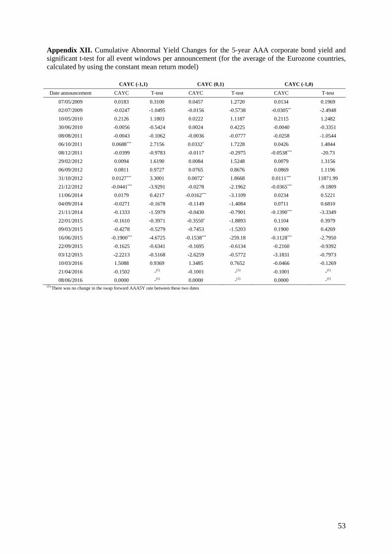
53

Appendix XII. Cumulative Abnormal Yield Changes for the 5-year AAA corporate bond yield and



CAYC (-1,1) CAYC (0,1) CAYC (-1,0)


07/05/2009 0.0183 0.3100 0.0457 1.2720 0.0134 0.1969

02/07/2009 -0.0247 -1.0495 -0.0156 -0.5738 -0.0305** -2.4948

10/05/2010 0.2126 1.1803 0.0222 1.1187 0.2115 1.2482

30/06/2010 -0.0056 -0.5424 0.0024 0.4225 -0.0040 -0.3351

08/08/2011 -0.0043 -0.1062 -0.0036 -0.0777 -0.0258 -1.0544

06/10/2011 0.0688*** 2.7156 0.0332* 1.7228 0.0426 1.4844

08/12/2011 -0.0399 -0.9783 -0.0117 -0.2975 -0.0538*** -20.73

29/02/2012 0.0094 1.6190 0.0084 1.5248 0.0079 1.3156

06/09/2012 0.0811 0.9727 0.0765 0.8676 0.0869 1.1196

31/10/2012 0.0127*** 3.3001 0.0072* 1.8668 0.0111*** 11871.99

21/12/2012 -0.0441*** -3.9291 -0.0278 -2.1962 -0.0365*** -9.1809

11/06/2014 0.0179 0.4217 -0.0162*** -3.1109 0.0234 0.5221

04/09/2014 -0.0271 -0.1678 -0.1149 -1.4084 0.0711 0.6810

21/11/2014 -0.1333 -1.5979 -0.0430 -0.7901 -0.1390*** -3.3349

22/01/2015 -0.1610 -0.3971 -0.3550* -1.8893 0.1104 0.3979

09/03/2015 -0.4278 -0.5279 -0.7453 -1.5203 0.1900 0.4269

16/06/2015 -0.1900*** -4.6725 -0.1538*** -259.18 -0.1128*** -2.7950

22/09/2015 -0.1625 -0.6341 -0.1695 -0.6134 -0.2160 -0.9392

03/12/2015 -2.2213 -0.5168 -2.6259 -0.5772 -3.1831 -0.7973

10/03/2016 1.5088 0.9369 1.3485 0.7652 -0.0466 -0.1269

21/04/2016 -0.1502 -(1) -0.1001 -(1) -0.1001 -(1)

08/06/2016 0.0000 -(1) 0.0000 -(1) 0.0000 -(1) (1)

There was no change in the swap forward AAA5Y rate between these two dates

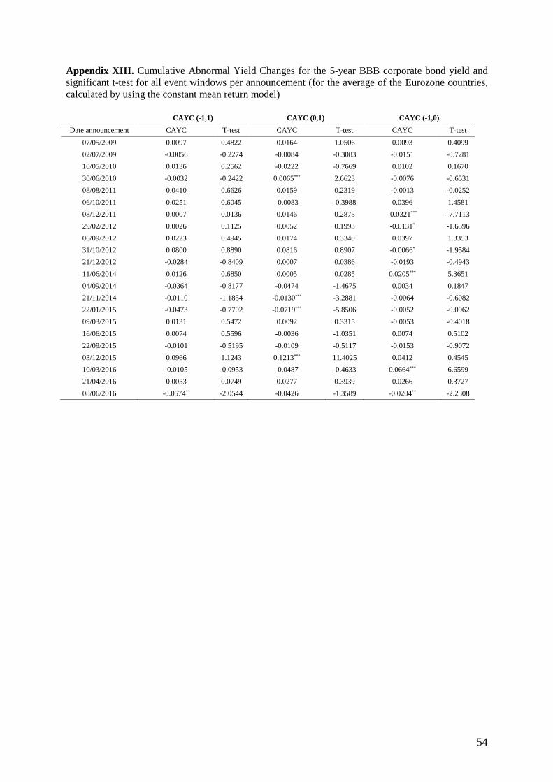
54

Appendix XIII. Cumulative Abnormal Yield Changes for the 5-year BBB corporate bond yield and



CAYC (-1,1) CAYC (0,1) CAYC (-1,0)


07/05/2009 0.0097 0.4822 0.0164 1.0506 0.0093 0.4099

02/07/2009 -0.0056 -0.2274 -0.0084 -0.3083 -0.0151 -0.7281

10/05/2010 0.0136 0.2562 -0.0222 -0.7669 0.0102 0.1670

30/06/2010 -0.0032 -0.2422 0.0065*** 2.6623 -0.0076 -0.6531

08/08/2011 0.0410 0.6626 0.0159 0.2319 -0.0013 -0.0252

06/10/2011 0.0251 0.6045 -0.0083 -0.3988 0.0396 1.4581

08/12/2011 0.0007 0.0136 0.0146 0.2875 -0.0321*** -7.7113

29/02/2012 0.0026 0.1125 0.0052 0.1993 -0.0131* -1.6596

06/09/2012 0.0223 0.4945 0.0174 0.3340 0.0397 1.3353

31/10/2012 0.0800 0.8890 0.0816 0.8907 -0.0066* -1.9584

21/12/2012 -0.0284 -0.8409 0.0007 0.0386 -0.0193 -0.4943

11/06/2014 0.0126 0.6850 0.0005 0.0285 0.0205*** 5.3651

04/09/2014 -0.0364 -0.8177 -0.0474 -1.4675 0.0034 0.1847

21/11/2014 -0.0110 -1.1854 -0.0130*** -3.2881 -0.0064 -0.6082

22/01/2015 -0.0473 -0.7702 -0.0719*** -5.8506 -0.0052 -0.0962

09/03/2015 0.0131 0.5472 0.0092 0.3315 -0.0053 -0.4018

16/06/2015 0.0074 0.5596 -0.0036 -1.0351 0.0074 0.5102

22/09/2015 -0.0101 -0.5195 -0.0109 -0.5117 -0.0153 -0.9072

03/12/2015 0.0966 1.1243 0.1213*** 11.4025 0.0412 0.4545

10/03/2016 -0.0105 -0.0953 -0.0487 -0.4633 0.0664*** 6.6599

21/04/2016 0.0053 0.0749 0.0277 0.3939 0.0266 0.3727

08/06/2016 -0.0574** -2.0544 -0.0426 -1.3589 -0.0204** -2.2308