1

The simulation of free surface flows with Computational Fluid Dynamics B. Godderidge1 A.B. Phillips, S. Lewis, S.R. Turnock, D.A. Hudson, and M. Tan. Fluid-Structure Interactions Research Group, Froude Building, School of Engineering Sciences, University of Southampton, SO17 1BJ, UK. SUMMARY Computational fluid dynamics is a powerful and versatile tool for the analysis of flow problems encountered in the maritime environment. The University of Southampton Fluid-Structure Interactions research group use ANSYS CFX to model a wide variety of flow problems; to gain insight into flow physics, improve designs and increase the efficiency and safety of marine vehicles. A series of three case studies from on-going research looks at: loads applied on liquefied natural gas tanks due to sloshing, slamming pressures experienced by high speed craft as well as the influence of propellers on the resistance characteristics of autonomous underwater vehicles. The presence of the free surface, complex shapes and the unsteady nature of these applications make their simulation with computational fluid dynamics particularly challenging. The successful validation of the computational models has resulted in the development of a selection process for suitable multiphase models as well as cost-effective meshing strategies. 1. INTRODUCTION Cutting-edge designs, ambitious operating profiles and greater emphasis on the environmental impact of marine vehicles is resulting in the increased use of Computational Fluid Dynamics (CFD) – the numerical solution of the Navier-Stokes equations – in naval architecture. The key complication in the application of CFD in the marine field is the presence of an interface between water and air (free surface). Since the position of the free surface is not known a priori, it must be obtained as part of the solution process. A wide variety of solution methods have been developed to deal with this problem. Marker-and-cell methods keep track of the free surface position. This is computationally efficient, but does not permit overturning waves or fluid fragmentation. Particle methods resolve the flow into a finite number of fluid elements. This approach is robust, but it consumes a large amount of computational power. Hirt and Nichols (1981) developed a free surface capturing approach for finite volume CFD, where the amount of each fluid in a control volume is calculated in the solution process. Although this approach is computationally expensive it is robust and permits the simulation of highly non-linear free surface shapes, including fluid fragmentation and wave breaking. Most commercial CFD codes, including CFX, use this approach to include a free surface flow modelling capability. The Fluid-Structure Interactions Research Group at the University of Southampton use ANSYS CFX to model a wide variety of free surface flow problems such as sloshing, self-propulsion and high speed craft slamming loads to gain insight into flow physics, improve designs and increase the efficiency and safety of marine vehicles.

The application and validation of CFD in this wide variety of maritime free surface flows has resulted in the identification of easily applied guidelines for the selection of an appropriate multiphase model, the construction of sufficiently robust meshes as well as an analysis of the free surface modelling capabilities in CFX. 2. VIOLENT SLOSHING IN LNG CARRIERS 2.1 THE ENGINEERING PROBLEM Natural gas has become a popular solution to satisfy the energy needs of the world and the requirements for gas shipping have consequently increased. Royal Dutch Shell expects the LNG market to grow to the same size as the petroleum market by 2025 (The Economist, 2004) as power generation and industry as well as households increase their reliance on natural gas The transport of Liquefied Natural Gas (LNG) by ship over transoceanic distances is more cost effective than

Figure 1 – Every second matters: high-performance engineering to save lives (Photo courtesy of RNLI)

____________________________________________

1 email: bg401@soton.ac.uk

2

the construction and operation of pipelines (Jensen, 2002). Sloshing is a danger to the safety of LNG carriers, but it is usually avoided by the judicious selection of tank size and filling level. However, the current economic climate in the global gas market has precipitated three principal developments challenging the status quo in the design of LNG carriers: 1. Increased Ship Size. The capacity of newbuild LNG

carriers is set to increase in excess of 250,000 m3. The LNG production and transport chains, commonly known as ‘LNG trains’, have increased in scale, requiring larger capacity vessels (Ginsburg and Bläske, 2007).

2. Flexible Filling Levels. This requirement is caused by a shift in the pattern of LNG trade. In the past, LNG ships were built for a certain LNG project with a fixed route. Today’s gas market is considerably more flexible and spot trading is starting to emerge as an alternative to the traditional trading arrangements (Crooks, 2007). Thus, energy companies seek to take advantage of local price variations.

3. Offshore Liquefaction and Gasification. The opposition to the construction of LNG liquefaction and regasification terminals has led to the development of floating LNG regasification plants. Due to the changing filling level of the LNG storage tanks and the seaway, sloshing is a key concern in the design and operation of floating LNG liquefaction and regasification (Mokhatab and Wood, 2007).

The significance of sloshing on the operation of LNG carriers is illustrated by an incident affecting the LNG carrier Catalunya Spirit. During dry dock inspection in May 2006, damage to the membrane tank insulation was discovered which was later attributed to sloshing. The repairs cost $4.1 million and the operator incurred a further $2.4 million loss, as the Catalunya Spirit remained in dry dock for repairs for 47 days (Teekay, 2006).

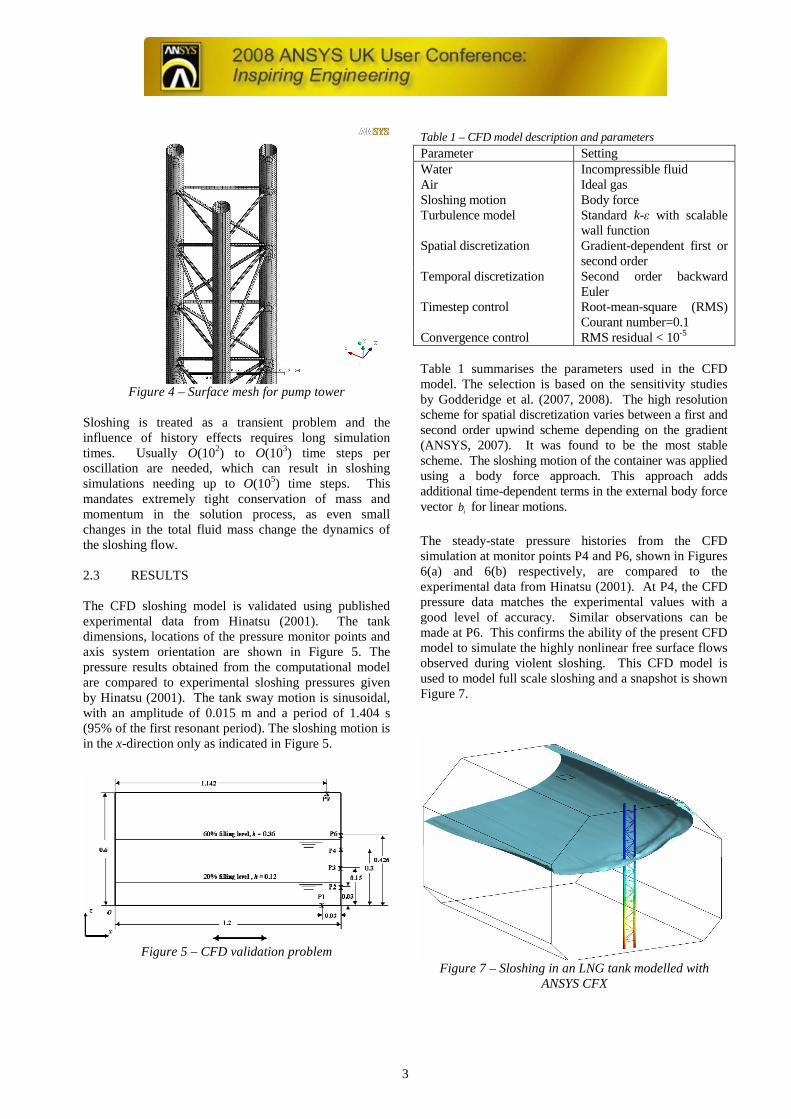
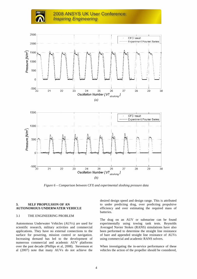
This has renewed interest in liquid sloshing and its effect on ship safety. CFD offers a cost-effective method of studying sloshing flows and analysing their impact on vessel operation. 2.2 SIMULATION CHALLENGES Although the shape of an LNG tank, shown in Figure 3, is readily discretised, the successful simulation of sloshing is complicated by numerous aspects. The pump tower, which is an integral part of LNG transportation is a complicated structure, which requires a large number of mesh elements for its adequate discretisation and resolution of the pressure field. A typical surface mesh for part of a pump tower is shown in Figure 4.

The highest pressure loads are encountered in sloshing flows with wave breaking, fluid fragmentation and air entrainment during impact. This requires robust numerical schemes which can handle large changes in the flow field over very short times. The separation between the phases and the “thickness” of the free surface influence the simulation results.

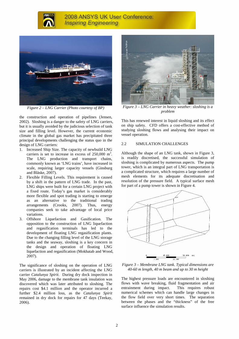
Figure 2 – LNG Carrier (Photo courtesy of BP)

Figure 3 – LNG Carrier in heavy weather: sloshing is a

problem

Figure 3 – Membrane LNG tank. Typical dimensions are

40-60 m length, 40 m beam and up to 30 m height

3

Sloshing is treated as a transient problem and the influence of history effects requires long simulation times. Usually O(102) to O(103) time steps per oscillation are needed, which can result in sloshing simulations needing up to O(105) time steps. This mandates extremely tight conservation of mass and momentum in the solution process, as even small changes in the total fluid mass change the dynamics of the sloshing flow. 2.3 RESULTS The CFD sloshing model is validated using published experimental data from Hinatsu (2001). The tank dimensions, locations of the pressure monitor points and axis system orientation are shown in Figure 5. The pressure results obtained from the computational model are compared to experimental sloshing pressures given by Hinatsu (2001). The tank sway motion is sinusoidal, with an amplitude of 0.015 m and a period of 1.404 s (95% of the first resonant period). The sloshing motion is in the x-direction only as indicated in Figure 5.

Table 1 summarises the parameters used in the CFD model. The selection is based on the sensitivity studies by Godderidge et al. (2007, 2008). The high resolution scheme for spatial discretization varies between a first and second order upwind scheme depending on the gradient (ANSYS, 2007). It was found to be the most stable scheme. The sloshing motion of the container was applied using a body force approach. This approach adds additional time-dependent terms in the external body force vector ib for linear motions.

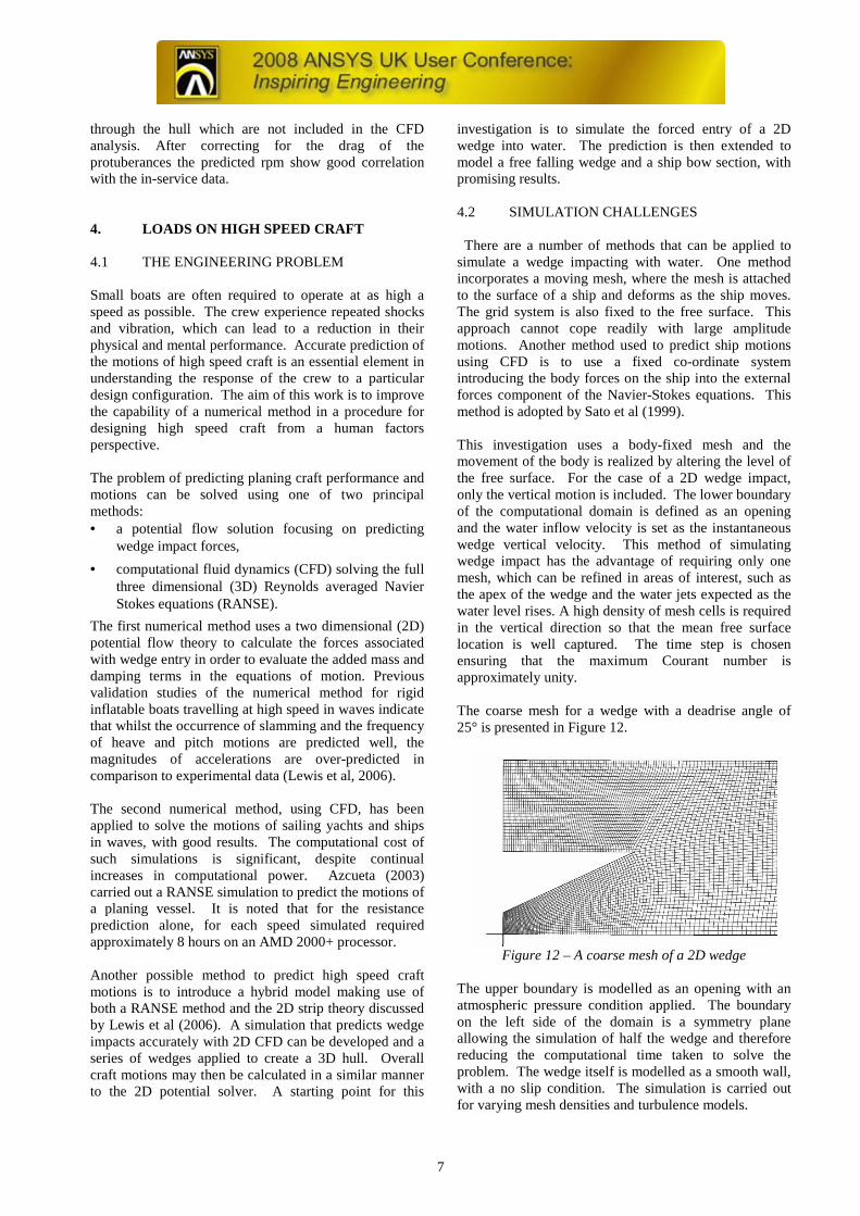
The steady-state pressure histories from the CFD simulation at monitor points P4 and P6, shown in Figures 6(a) and 6(b) respectively, are compared to the experimental data from Hinatsu (2001). At P4, the CFD pressure data matches the experimental values with a good level of accuracy. Similar observations can be made at P6. This confirms the ability of the present CFD model to simulate the highly nonlinear free surface flows observed during violent sloshing. This CFD model is used to model full scale sloshing and a snapshot is shown Figure 7.

Figure 4 – Surface mesh for pump tower

Figure 5 – CFD validation problem

Table 1 – CFD model description and parameters

Parameter Setting Water Incompressible fluid Air Ideal gas Sloshing motion Body force Turbulence model Standard k-ε with scalable

wall function Spatial discretization Gradient-dependent first or

second order Temporal discretization Second order backward

Euler Timestep control Root-mean-square (RMS)

Courant number=0.1 Convergence control RMS residual < 10-5

Figure 7 – Sloshing in an LNG tank modelled with

ANSYS CFX

4

(a)

(b)

Figure 6 – Comparison between CFX and experimental sloshing pressure data

3. SELF PROPULSION OF AN AUTONOMOUS UNDERWATER VEHICLE 3.1 THE ENGINEERING PROBLEM Autonomous Underwater Vehicles (AUVs) are used for scientific research, military activities and commercial applications. They have no external connections to the surface for powering, mission control or navigation. Increasing demand has led to the development of numerous commercial and academic AUV platforms over the past decade (Phillips et al, 2008). Stevenson et al (2007) note that many AUVs do not achieve the

desired design speed and design range. This is attributed to under predicting drag, over predicting propulsive efficiency and over estimating the required mass of batteries. The drag on an AUV or submarine can be found experimentally using towing tank tests. Reynolds Averaged Navier Stokes (RANS) simulations have also been performed to determine the straight line resistance of bare and appended straight line resistance of AUVs using commercial and academic RANS solvers. When investigating the in-service performance of these vehicles the action of the propeller should be considered,

5

since it modifies the surface pressure distribution and boundary layer flow at the stern of the vehicle with an associated change in hull resistance. Numerically the action of the marine propeller on the flow around a hull form can be included either by modelling explicitly the full rotating propeller in an unsteady RANS simulation of the hull-propeller system; or by modelling the hull with a propeller model based on an actuator-disc approach. A typical AUV propeller, like a ship model propeller, will often operate in the transition Reynolds Number range and use of a standard RANS approach may well not capture the behaviour of the propeller.

In order to better understand the in-service performance of AUVs the self-propelled free flying condition of the AUV Autosub 3, shown in Figure 8, is simulated with the commercial RANS solver ANSYS CFX V11. The propeller is modelled using an extended actuator disc approach using blade element momentum theory (BEMT) to determine the required axial and tangential momentum source terms. The eventual aim is to provide a cost effective analysis technique for developing new AUVs. 3.2 AUTOSUB 3 Autosub 3 is a torpedo shaped AUV manoeuvred by four identical flapped control surfaces mounted at the rear of the vessel, in a cruciform arrangement, Figure 9. Two vertical rudders control the yaw of the vessel, while two horizontal sternplanes adjust the pitch. The full skeg foils use a NACA0015 section with a tip chord of 270mm, root chord of 368mm and a span of 386mm. The movable flap has a chord of 185mm and a span of 330mm. The propulsion system consists of a single brushless DC motor that directly drives a two bladed aluminium alloy propeller, positioned at the rear of the vessel behind the control surfaces. The blades are 240mm long with a chord of 35mm, diameter 0.7m with a hub/diameter ratio of 0.3486.

3.3 COUPLED RANS-BEMT SIMULATION Blade element momentum theory (BEMT) is commonly used in the design of turbines and marine propellers. The advantage of BEMT theory over more advanced methods is that it allows the lift and drag properties of the 2D section to be tuned to the local Reynolds number incorporating viscous effects such as stall or the effect of laminar separation at low Reynolds numbers. An existing compact BEMT code written at the University of Southampton has been modified to simulate the action of Autosub’s propeller. The 2D lift and drag data calculated from XFoil has been modelled including the Reynolds number dependent drag coefficient. The propeller sideforce can lead to large moments due to the distance between the propeller and the Autosub centre of gravity (0.47L). In order to capture the radial and circumferential variation in propeller inflow conditions are determined for 360 discrete zones (10 radial divisions, 36 circumferential divisions), see Figure 9. The BEMT code is called for each of these locations to determine the local thrust and torque coefficients.

Figure 9 – 36 circumferential and 10 radial subdivisions

of the propeller disk Within the RANS simulation the propeller is modelled as a cylindrical subdomain with a diameter equal to that of the propeller and a length equal to that of the rotating hub, 0.069D. Momentum source terms are then applied over the subdomain in cylindrical coordinates to represent the axial and tangential momentum induced by the propeller. An iterative approach is used to establish the self propulsion point.

Figure 8 – Launch of the 7m Autonomous Underwater

Vehicle Autosub 3

6

This approach is implemented through the use of a CFX Junction Box Routine and CFX User Fortran Routines. The Junction Box routine is called at the end of every coefficient loop. It monitors convergence levels, extracts wake data and controls the set propeller rpm. The Fortran Routines are used to run the BEMT code based on the wake data and rpm from the Junction Box Routine, in order to determine the momentum source distribution and return the appropriate source terms to CFX. The computational cost of running the BEMT code at each coefficient loop is 0.1% of the cost of the RANS simulation. 3.4 RESULTS The coupled RAN-BEMT simulation estimates a propeller rpm of 294 for self propulsion at 2m/s. This value is substantially lower than the rpm values seen in-service, Figure 11. There are two possible causes of this discrepancy; over prediction of thrust in the BEMT code or under prediction of the vehicle drag in the RANS simulation.

Using the ITTC 57 correlation line, and a form factor from Hoerner (1965) for a streamlined body the bare hull drag coefficient can be estimated as CDV = 0.02219 compared with CDV = 0.0215 derived from the RANS simulation. The four control surfaces add an extra 13% to the drag leading to a CDV = 0.024, lower than the accepted value for Autosub derived from deceleration tests of CDV = 0.045 The discrepancies between the numerical and in service drag is believed to be due to the various instruments and antennae with project through Autosub’s hull, see Figure 8, these protuberances have been ignored in the numerical simulations. Allen et al. (2000) performed towing tank tests to determine the relative contribution of hull, fins, transducers and nose pockets to the total hydrodynamic drag of a REMUS AUV. The results identified the transducer and nose pockets comprised

nearly half of the total drag of the vehicle, thus highlighting that the drag of the basic hull is often not the major contributor to the total drag of an AUV and underlining the need for including a high level of detail in both experiment and simulation. Taking the wake fraction and thrust deduction calculated by the RANS-BEMT simulation, and replacing the drag calculated from the RANS analysis with that calculated using the drag coefficient CDV = 0.045 the resulting prediction of rpm versus water speed are presented on Figure 11. These show good agreement with the in service data confirming the analysis undertaken. 3.5 OUTCOMES A robust and rapid method of coupling a Blade Element Momentum theory code for marine propellers with the commercial RANS code ANSYS CFX has been developed. The computational cost of running the BEMT code at each coefficient loop is 0.1% of the cost of the RANS simulation, and thus significantly lower than modelling the propeller blade in the RANS simulation explicitly. Viscous effects such as stall or low Reynolds number effects such as laminar separation can be included when defining the lift and drag properties of the 2D sections. Radial and circumferential variation in propeller performance can be captured by considering the local inflow conditions at a series of radial and circumferential divisions. This allows for non uniform propeller inflow such as that observed behind a ship or submarine. Self propulsion simulations using the RANS-BEMT method have been performed over the range of operational Reynolds numbers for the AUV Autosub 3. Hull efficiency is shown to decrease with Reynolds number while the propeller open water efficiency increases. Comparisons with in service data show the RANS-BEMT simulation under predicts the drag of the vehicle and consequently the required rpm. This is attributed to the various instruments and antennae which protrude

Figure 10 – Streamlines around the vehicle at a nose down pitch angle of 4 deg and a sternplane angle of

6_deg

Figure 11 – RPM versus water speed, (Mission data

from Autosub Missions 385, 386 and 387)

7

through the hull which are not included in the CFD analysis. After correcting for the drag of the protuberances the predicted rpm show good correlation with the in-service data. 4. LOADS ON HIGH SPEED CRAFT 4.1 THE ENGINEERING PROBLEM Small boats are often required to operate at as high a speed as possible. The crew experience repeated shocks and vibration, which can lead to a reduction in their physical and mental performance. Accurate prediction of the motions of high speed craft is an essential element in understanding the response of the crew to a particular design configuration. The aim of this work is to improve the capability of a numerical method in a procedure for designing high speed craft from a human factors perspective. The problem of predicting planing craft performance and motions can be solved using one of two principal methods: • a potential flow solution focusing on predicting

wedge impact forces,

• computational fluid dynamics (CFD) solving the full three dimensional (3D) Reynolds averaged Navier Stokes equations (RANSE).

The first numerical method uses a two dimensional (2D) potential flow theory to calculate the forces associated with wedge entry in order to evaluate the added mass and damping terms in the equations of motion. Previous validation studies of the numerical method for rigid inflatable boats travelling at high speed in waves indicate that whilst the occurrence of slamming and the frequency of heave and pitch motions are predicted well, the magnitudes of accelerations are over-predicted in comparison to experimental data (Lewis et al, 2006). The second numerical method, using CFD, has been applied to solve the motions of sailing yachts and ships in waves, with good results. The computational cost of such simulations is significant, despite continual increases in computational power. Azcueta (2003) carried out a RANSE simulation to predict the motions of a planing vessel. It is noted that for the resistance prediction alone, for each speed simulated required approximately 8 hours on an AMD 2000+ processor. Another possible method to predict high speed craft motions is to introduce a hybrid model making use of both a RANSE method and the 2D strip theory discussed by Lewis et al (2006). A simulation that predicts wedge impacts accurately with 2D CFD can be developed and a series of wedges applied to create a 3D hull. Overall craft motions may then be calculated in a similar manner to the 2D potential solver. A starting point for this

investigation is to simulate the forced entry of a 2D wedge into water. The prediction is then extended to model a free falling wedge and a ship bow section, with promising results. 4.2 SIMULATION CHALLENGES There are a number of methods that can be applied to simulate a wedge impacting with water. One method incorporates a moving mesh, where the mesh is attached to the surface of a ship and deforms as the ship moves. The grid system is also fixed to the free surface. This approach cannot cope readily with large amplitude motions. Another method used to predict ship motions using CFD is to use a fixed co-ordinate system introducing the body forces on the ship into the external forces component of the Navier-Stokes equations. This method is adopted by Sato et al (1999). This investigation uses a body-fixed mesh and the movement of the body is realized by altering the level of the free surface. For the case of a 2D wedge impact, only the vertical motion is included. The lower boundary of the computational domain is defined as an opening and the water inflow velocity is set as the instantaneous wedge vertical velocity. This method of simulating wedge impact has the advantage of requiring only one mesh, which can be refined in areas of interest, such as the apex of the wedge and the water jets expected as the water level rises. A high density of mesh cells is required in the vertical direction so that the mean free surface location is well captured. The time step is chosen ensuring that the maximum Courant number is approximately unity. The coarse mesh for a wedge with a deadrise angle of 25° is presented in Figure 12.

Figure 12 – A coarse mesh of a 2D wedge

The upper boundary is modelled as an opening with an atmospheric pressure condition applied. The boundary on the left side of the domain is a symmetry plane allowing the simulation of half the wedge and therefore reducing the computational time taken to solve the problem. The wedge itself is modelled as a smooth wall, with a no slip condition. The simulation is carried out for varying mesh densities and turbulence models.

8

The simulation of a free falling wedge requires the inflow velocity to vary according to the vertical force on the wedge. In order to calculate the new velocity, the velocity at the previous time step must be known. A FORTRAN program was integrated within the CFD simulation. At each time step the total vertical force acting on the wedge is known and using the wedge mass, a new velocity can be found as:

tM

FgWW OLDNEW ∆

−+= .

The velocity at the previous time step is retrieved from a text file. This new velocity is then returned to the CFD solver and implemented in the inlet boundary conditions. The velocity is also used to over-write the text file for use in the next time step. As the necessary time step for the CFD simulation is sufficiently small a simple first order calculation is sufficiently accurate. 4.3 OUTCOMES 4.3.1 2D Wedge impact Initial inspection of the results is conducted in a qualitative manner. The free surface is inspected to ensure that a reasonably sharp interface is predicted with a rapid variation of volume fraction across 3 to 5 cells only. Figure 13 illustrates a typical free surface mid way through a simulation for the coarse mesh showing a contour plot of the water volume fraction. This was deemed acceptable with clear identification both of the wedge jet and mean water level.

Figure 13 – Contour plot of the water volume fraction

illustrating the free surface.

A mesh and turbulence model sensitivity study was carried out, with meshes ranging from 9,000 cells to 52,000 cells. The predictions are compared with experimental data from tests conducted by Yettou et al (2006). Figure 14 presents the computed prediction of the pressure distribution along the wedge at 4 different times. These times correspond to the maximum pressure experienced by transducers 1, 3, 5 and 6. The time is set to zero when the wedge first touches the water. It is noted that each pressure transducer has a diameter of 19mm. Therefore the average maximum pressure over a 19mm section of the wedge must also be considered. The peak pressures are presented in Figure 14 as well as the average maximum pressure at the position of each transducer. Peak pressures are under-predicted near the wedge apex, as is the averaged pressure. The pressures are over predicted as the water jet travels up the wedge and the averaged pressure follows the same trend, although with increased accuracy.

0.0E+00

2.0E+04

4.0E+04

6.0E+04

8.0E+04

1.0E+05

1.2E+05

1.4E+05

0 0.05 0.1 0.15 0.2 0.25 0.3 0.35 0.4y (m)

Pre

ssu

re (P

a)

Experimental pressure peaks

Predicted pressure t=2.5ms

Predicted pressure t = 8ms

Predicted Pressure t = 17.5ms

Predicted pressure t = 23ms

Averaged predicted maximum

Figure 14 – Predicted pressure distribution along the

wedge face, with averaged maximum pressure and experimental data.

The contour plots of the pressure in the fluid around the wedge at different times are illustrated in Figure 15. These illustrate the pressure peak moving along the wedge during impact, as well as the reduction in peak pressure with time.

9

While the prediction of pressures acting on the wedge is important, the forces acting on the wedge and its subsequent motions are of primary concern in this study. Figure 16 illustrates the accuracy of various potential flow theories when compared to the experimental results and the current CFD predictions.

1

1.5

2

2.5

3

3.5

4

4.5

5

0 5 10 15 20 25 30 35 40

Time (ms)

Spe

ed (

m/s

)

Computational Prediction

Zhao's model

Experimental data: Yettou et al(2006)

Von Karman Model

Zarnick Model

Wagner Model

Figure 16 – Comparison between computational

prediction, experimental data and various potential flow solutions.

4.3.2 Hull bow section impact Although the potential flow theories discussed in section 4.3.1 produce reasonable results for constant deadrise wedges, they are not capable of solving the problem for more complex bodies. This section presents an overview of work conducted on the impact of a ship bow section with water. The experiment is conducted by Aarsnes

(1996). The bow section with pressure tappings is illustrated in Figure17

Figure 17 - Diagram of ship bow section (Aarsnes, 1996)

Figure 18 – Mesh for the ship bow section. Three meshes of the bow section were created, each with a length of 0.8m and a height of 0.4m. The finest mesh contained 30000 cells, and the first node was situated

5102 −⋅ m from the wall of the bow section (see Figure 18). The time step is varied from 0.5ms to 0.05ms. The details of the method for the CFD simulation can be found in Hudson et al (2007). The peak impact pressures are captured well, although are under predicted by up to 10% as presented in Figure 19 The accurate modelling of an unsteady boundary layer allows improvements in the prediction of a body impacting with water. The results presented demonstrate that such a CFD approach predicts the magnitude and time history of the pressure distribution accurately as compared to available experimental data. The results presented illustrate an improvement over potential flow theory predictions.

Figure 15 – Pressure contours around the wedge: clockwise from top left, t=2.5ms; t=8ms; t=23ms;

t=17.5ms.

10

5. FREE SURFACE MODELLING 5.1 WHAT MULTIPHASE MODEL? In the case studies in Sections 2-4, the interaction between the fluids at the free surface behaviour directly influences the results and a suitable multiphase model for capturing the free surface dynamics needs to be identified. The fluid interaction models for the numerical simulation of free surface flows can be implemented using the volume fraction of each fluid to determine the fluid mixture properties. This is a homogeneous multiphase model which is analogous to the volume of fluid (VOF) method developed by Hirt and Nichols (1981). A more general but computationally more expensive approach is an inhomogeneous multiphase model, where the solution of separate velocity fields for each fluid is matched at the fluid interfaces using mass and momentum transfer models (Ishii and Hibiki, 2006) The physics of a violent free surface flows such as sloshing, including wave breaking, vapour entrapment and cushioning may contradict the assumptions (Brennen, 2005) inherent in the homogeneous model. An inhomogeneous viscous compressible multiphase flow with two phases α and β can be described by the conservation of mass for the compressible phase α

( ) ( ) ,= αβρρ Γ+∂∂+

∂∂

murx

rt i

i

(1)

where αβΓ is mass transfer between the phases and m mass sources, ρ density, r volume fraction and iu

velocity of phase α . The corresponding equation for conservation of momentum for phase α is given as

( ) ( )( )

,

=

ij

ij

i

jij

i

bMMx

r

x

pr

uurx

urt

+++∂

∂+

∂∂−=

∂∂+

∂∂

Γ ατ

ρρ

(2)

where ib are body forces, αM forces on the interface

caused by the presence of phase β , µ the dynamic

viscosity, the term ( )ii uuM βαβαβ Γ−ΓΓ = interphase

momentum transfer caused by mass transfer and the stress tensor ijτ is expressed as

∂∂

+∂∂

i

j

j

iij x

u

x

uµτ = (3)

The interface momentum transfer term αM needs to be considered in greater detail as it links the fluid velocity fields. This term may be modelled by a linear combination of known forces acting on the fluid interface, such that

,= WLBVD MMMMMM ++++α (4)

where DM is drag force, VM virtual mass force, BM

Basset force, LM lift force due to fluid rotation and WM wall lubrication force (Ishii and Hibiki, 2006). Due

to its complicated nature, the Basset force is generally ignored in practical multiphase analysis (Ishii and Hibiki, 2006). The virtual mass force is used to model the interaction of small, subgrid-scale particles with the surrounding fluid. This is ignored in the present analysis. The lift force is generated by fluid rotation around particles. The correct modelling of wall lubrication force requires a fine grid (Ishii and Hibiki, 2006), making its inclusion in transient simulations impractical. The

interphase drag force DM is expressed using the drag coefficient

,1/2

=2

AUU

DCD

βαρ − (5)

where A is interfacial area, D drag, ρ density and

βα UU − velocity between the phases α and β . For

the current Newtonian flow regime, a drag coefficient of 0.45 is used (Ishii and Hibiki, 2006). Equations (1) and (2) are computationally expensive as the number of conservation equations to be solved doubles with an additional fluid. A simplification is given with homogeneous multiphase flow. In this case it is assumed that the relative motion between the phases can be neglected (Brennen, 2005). Thus, the interface momentum transfer in Equation (4) becomes large, but the velocity field is identical for both phases and only one set of conservation of momentum equations needs to be solved. Applying this simplification to the governing equations for inhomogenous multiphase flow, conservation of mass for homogeneous multiphase flow is given as

Predicted and experimental pressure (transducers P1 and P2)

-5000

0

5000

10000

15000

20000

25000

30000

35000

-0.02 0 0.02 0.04 0.06 0.08 0.1

Time (s)

Pre

ssur

e (P

a)

P1 pressure prediction

P1 experiment

P2 Pressure prediction

P2 experiment

Figure 19 – Pressure predictions compared with experimental data from pressure transducers P1 and P2

11

( ) ( ) 0,=ii

urxt

r ρρ∂∂+

∂∂

(6)

and the conservation of momentum is defined as

( ) ( ) ij

ij

iji

ji b

xx

puu

xu

t+

∂∂

+∂∂−

∂∂+

∂∂ τ

µρρ = (7)

with

lll

r ρρ ∑2

1=

= (8)

and

.=2

1=ll

l

r µµ ∑ (9)

In considering computational efficiency alone, the homogeneous multiphase model will be the most effective but the interaction between the phases is ignored. The homogeneous multiphase model is used in most sloshing simulations. When the water impacts a tank wall, a small air pocket usually remains. This behaviour is observed in experimental studies of sloshing (e.g. Lugni et al, 2006) as well as the present computational investigation. The properties of this bubble and surrounding fluid can be used to determine a suitable multiphase model. Brennen (2005) provides guidance using a size parameter X and a mass parameter Y in conjunction with the particle Reynolds number. They are defined as

,1=v

m

l

RX

c

p

ρ− (10)

+−

v

m

v

mY

c

p

c

p

ρρ2

1/1= (11)

and the particle Reynolds number

α

αβα ν

RUURN

−=, , (12)

wherel is length scale, pm particle mass, cν kinematic

viscosity, cρ fluid density, R particle radius, U

characteristic velocity and v particle volume. Brennen

[22] finds that if either the condition 2<<YX or )//(<< cURYX ν is violated, the inhomogeneous

multiphase model (Equations 1 and 2) should be used. 5.2 COMPUTATIONAL GRID The size and nature of the mesh used in free surface simulations affects the solution process as well as the quality of the results. Tetrahedral (tetra) grids are relatively straightforward to generate, and when

combined with inflation layers can capture boundary layers with no significant increase in computational workload. Disadvantages include poor reproducibility and the refinement can only be influenced by specifying mesh density and/or boundary node spacing. Hexahedral grids are significantly more complicated to generate but make more efficient use of a given number of nodes, especially when some knowledge of the flow is available.

Figure 20 – Typical hexa mesh of rectangular tank cross

section

Combining hexa and tetra elements in one grid is more complicated, but there are considerable advantages

• When conducting parametric variations only the inner region has to be regenerated – better repeatability and less effort, with an invariant far-field region.

• Reduction in the number of hexa elements while an orthogonal grid structure is maintained.

• Free surface modelling is sensitive to grid aspect ratio, with an aspect ratio greater than O(101) often resulting in computational instability or poor convergence. A hybrid grid can be used to maintain a low aspect ratio near the free surface while limiting the total number of grid elements.

• Transient runs are more sensitive to grid size, as the steady-state solution has to be obtained for each transient time step. Given that some applications such as sloshing require O(103-105) time steps, the additional effort in grid generation is justified.

Figure 20 shows the pure hexa mesh used for the sloshing simulation. Near the tank walls, the cell aspect

Figure 21 – Hybrid mesh of the same cross section as in Figure 20. 58% of the total elements are located in the

corners

12

ratio is in excess of 100 and convergence was often difficult to achieve. The same problem is discretised using a hybrid mesh approach in Figure 21. In this case, the mesh elements are distributed far more efficiently and a suitable aspect ratio is maintained outside the boundary layer regions. 6. CONCLUDING REMARKS Computational Fluid Dynamics is a powerful tool for the analysis and design of marine vehicles. For safety-critical aspects of their design and operation such as LNG sloshing and slamming pressure loads, CFD can provide insights and facilitate better designs. CFD is also useful when assessing the influence of changes to a design and optimising propulsion in conditions difficult to replicate in model tests. The successful simulation of free surface flows depends on the selection of an appropriate multiphase model and a methodology has been developed by Godderidge et al (2008). Hybrid grid make more economical free surface flow simulations possible, as they combine the advantages associated with hexahedral grids with low cell aspect ratios near the free surface. 7. ACKNOWLEDGEMENTS This work was carried out under the auspices of the Engineering Doctorate and PhD programmes at the University of Southampton, with support from the

Engineering and Physical Sciences Research Council (UK), BMT SeaTech Ltd, the Wolfson Unit for Marine Technology and Industrial Aerodynamics and the National Oceanography Centre (Southampton). The authors acknowledge the support in the scope of project MARSTRUCT, Network of Excellence on Marine Structures 4 financed by the European Union through the growth programme. The authors also wish to thank Ivan Wolton for his work managing the Iridis 2 computational facility which was used to carry out the bulk of the simulations presented in this paper. REFERENCES 1 Aarsnes J.J. (1996) Drop test with ship sections –

effect of roll angle. MARINTEK report number 603834.00.01.

2 Akimoto, A. and Miyata, H., (2002). Finite-volume simulation to predict the performance of a sailing boat. Journal of Marine Science and Technology 7 pp 31-42.

3 Allen B., Vorus, W.S., and Presreo, T. (2000). Propulsion system performance enhancements on REMUS AUVs. In OCEANS 2000 MTS/IEEE Conference and Exhibition.

4 ANSYS Inc (2007). ANSYS CFX-11 User’s Guide. 5 Azcueta, R. (2002) RANSE simulations for sailing

yachts including dynamic sinkage & trim and unsteady motions in waves. High Performance Yacht Design Conference, Auckland.

6 Brennen, C.E. (2005), Fundamentals of Multiphase Flow, Cambridge University Press, New York.

7 Ginsburg, H-J. and Bläske, G. (2007). Wir können sparen: Interview with Claude Mandil, International Energy Agency Executive Director. WirtschaftsWoche, 26 pp 26–29.

8 Godderidge, B, Tan, M, Earl, C and Turnock, S (2007). Boundary layer resolution for modeling of a sloshing liquid. Intl Soc Offshore and Polar Engrs Conf.

9 Godderidge, B, Turnock, S, Tan, M and Earl, C (2008) An Investigation of Multiphase CFD modelling of a lateral sloshing tank. Computers and Fluids (in print).

10 Hinatsu, M. (2001). Experiments of two-phase flows for the joint research. Proc of SRI-TUHH mini-Workshop on Numerical Simulation of Two-Phase Flows. National Maritime Research Institute & Technische Universität Hamburg-Harburg.

11 Hirt, C.W. and Nichols, B.D. (1981). Volume of fluid (VOF) method for the dynamics of free boundaries, Journal of Computational Physics, 39, pp 201–225.

12 Hoerner, S.F. (1965). Fluid Dynamic Drag. Published by the Author.

13 Hudson, D.A., Turnock S.. and Lewis S.G., 2007. Predicting motions of high-speed rigid inflatable boats: Improved wedge impact prediction, Proceedings of the Ninth International Conference on Fast Sea Transportation FAST2007, Shanghai, China, September.

14 Ishii M and Hibiki, T. (2006). Thermo-Fluid Dynamics of Two-Phase Flow, Springer Verlag.

15 Jensen, J.T. (2002). LNG and pipeline economics. In The Geopolitics of Gas Meeting. James A. Baker III Institute for Public Policy, Rice University and Program on Energy and Sustainable Development, Stanford University.

16 Lewis, S.G., Hudson, D. A., Turnock, S. R., Blake, J. I. R. and Shenoi, R. A. (2006) Predicting Motions of High Speed RIBs: A Comparison of Non-linear Strip Theory with Experiments. Proceedings of the 5th International Conference on High Performance Marine Vehicles (HIPER '06) pp 210-224.

17 Lugni, C., Brocchini, M., and Faltinsen, O.M. (2006) Wave impact loads: The role of the flip-through, Physics of Fluids 18 (12) 122101.

18 Mokhatab, S and Wood, D (2007). Breaking the offshore LNG stalemate. World Oil, 228(4), 2007.

19 Phillips, A.B., Furlong, M. and Turnock, S. (2008). Comparisons of CFD simulations and in-service data for the self-propelled performance of an autonomous underwater vehicle. 27th Symposium on Naval Hydrodynamics. Seoul, Korea, 5-10 October.

13

20 Sato, Y., Miyata, H., and Sato, T. (1999). CFD simulation of 3-dimensional motion of a ship in waves: application to an advancing ship in regular waves. Journal of Marine Science and Technology 4 pp 108-116.

21 Teekay LNG Partners LP. Annual Report. United States Securities and Exchange Commission, 2006.

22 The future’s a gas. (2004). The Economist, pp 53–54, 26 August.

23 Stevenson, P., Furlong, M., and Dormer, D. (2007). AUV shapes - combining the practical and hydrodynamic considerations. In Oceans 2007 Conference Proceedings.

24 Yettou, E-M., Desrochers, A. and Champoux, Y. (2006). Experimental study on the water impact of a symmetrical wedge. Fluid Dynamics Research 38 pp 47-66.