Embed Size (px)
Citation preview
1
EMC SeminarEMC Seminar
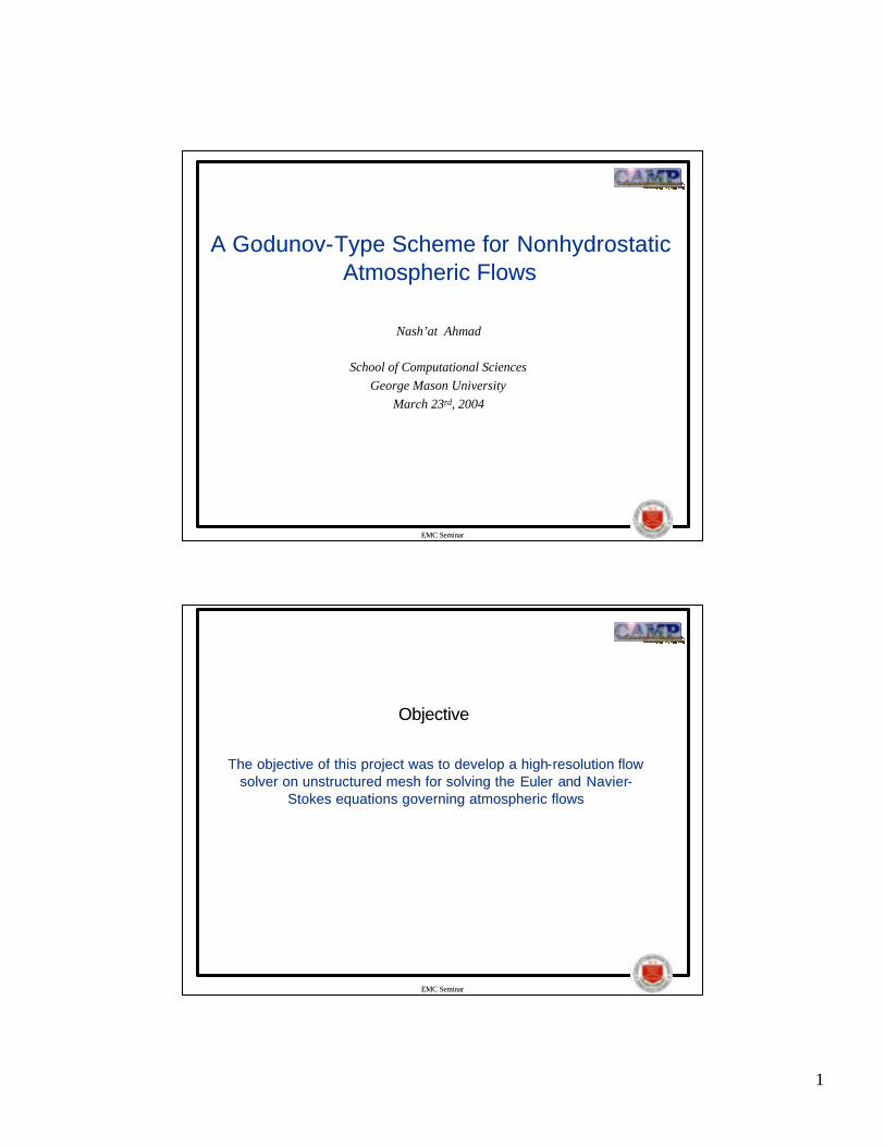
A A GodunovGodunov--Type Scheme for Type Scheme for NonhydrostaticNonhydrostaticAtmospheric FlowsAtmospheric Flows
Nash’at Ahmad
School of Computational SciencesGeorge Mason University
March 23rd, 2004
EMC SeminarEMC Seminar
ObjectiveObjective
The objective of this project was to develop a highThe objective of this project was to develop a high--resolution flow resolution flow solver on unstructured mesh for solving the solver on unstructured mesh for solving the Euler Euler and and NavierNavier--
Stokes equations governing atmospheric flowsStokes equations governing atmospheric flows

2
EMC SeminarEMC Seminar
OverviewOverview
• Background
• Properties of Euler Equations• Godunov Scheme• Harten-Lax-van Leer-Contact (HLLC) approximate Riemann
Solver (Toro et al.)• Monotone Upstream Schemes for Conservation Laws (MUSCL)• Comparison with other schemes• Implementation on Unstructured Meshes
• Results on Unstructured Meshes• Conclusions/Future Work
EMC SeminarEMC Seminar
ScalesScales
A Hierarchy of Atmospheric Forcings (from Bacon)
p∇Scenario Pressure
Change (mb)Horizontal Scale (km)
pressure gradient (mb/km)
Synoptic (meso-α) 10 1000 0.01
Mesoscale (meso-β) 10 100 0.10
Urban Scale – Light Winds (2kt) 0.006 0.05 0.12
Cloud Scale (meso-γ) 2 4 0.50
Land/Sea Boundary 1 1 1.00
Urban Scale – Thermal 2K Heat Island 24 20 1.20
Urban Scale – Strong Winds (10 kt) 0.16 0.05 3.20
Terrain Elevation ( 5% Grade) 5 1 5.00

3
EMC SeminarEMC Seminar
Why Unstructured Mesh ?Why Unstructured Mesh ?
• Provide continuous variable resolution
• Discretize complex geometries• Solution Adaptation – Efficient use of computational resources
EMC SeminarEMC Seminar
Atmospheric Applications on Unstructured MeshesAtmospheric Applications on Unstructured Meshes
•• Scalar TransportScalar Transport
• Ghorai, et al. (Godunov)
• Varvayani, et al. (FEM)
• Behrens, et al. (Semi-Lagrangian)
•• NavierNavier--Stokes EquationsStokes Equations
• Bacon et al. (Smolarkiewicz)

4
EMC SeminarEMC Seminar
Background Background –– Numerical SchemeNumerical Scheme
• Central finite difference schemes such as Leapfrog are favored
• Non-conservative discretizations• Exhibit large amounts of dispersion errors• Can generate false negatives in important scalars• Can become unstable in regions of high gradients• Time filters used to ensure stability often degrade the accuracy of
numerical results
EMC SeminarEMC Seminar
Possible CandidatesPossible Candidates
• Godunov-type schemes (Godunov, van Leer)
• Flux-Corrected Transport (Boris and Book)
• Central schemes (Jameson, Nessyahu-Tadmor)

5
EMC SeminarEMC Seminar
GodunovGodunov--Type SchemesType Schemes
• Hyperbolic Conservation Laws• Characteristics-based Conservative Finite Volume Discretizations• Numerical scheme based on the underlying physics of the
equations set• Extensively used in other scientific disciplines:
– Löhner, Luo et al., Lottati and Eidelman (CFD/Aerodynamics)– Wegman (MHD)– Ibáñez and Martí (relativistic astrophysics)– Vásquez -Cendón (shallow -water equations)
• Ability to resolve regions of high gradients:– Fronts– Drylines– Tornados– Hurricanes
• Exhibits minimal phase/dispersion errors• Numerical diffusion can be overcome by higher-order extensions
EMC SeminarEMC Seminar
GodunovGodunov--Type SchemesType Schemes

6
EMC SeminarEMC Seminar
GodunovGodunov--Type Schemes for Atmospheric Flow Type Schemes for Atmospheric Flow SimulationsSimulations
•• Scalar TransportScalar Transport
• Ghorai, et al. (Unstructured)
• Hubbard and Nikiforakis (Structured)
• Hourdin and Armengaud (Structured)
• Pietrzak (Structured)
•• Euler Euler EquationsEquations
• Carpenter et al. Godunov-PPM (Structured)
EMC SeminarEMC Seminar
Differences from Carpenter Differences from Carpenter etet al.al.
• The conservative equation set for modeling compressible flows inthe atmosphere is used, in which the conservation of energy is in terms of energy-density (ρθ) instead of entropy.
• The equations and the solution methodology are in the Eulerianframe of reference rather than Lagrangian.
• An approximate Riemann solver is employed instead of an exact solver to calculate the Godunov fluxes.
• Linear reconstruction of gradients instead of quadratic
• Finally, the scheme is extended to the Navier-Stokes equations (the sub-grid scale diffusion is treated as a source term) and implemented on unstructured meshes.

7
EMC SeminarEMC Seminar
NavierNavier--Stokes EquationsStokes Equations
Using conserved quantities (after Ooyama)
Dry adiabatic atmosphereThe only source term in Q is the gravitational force
DQyG
xF
tU +=
∂∂+
∂∂+
∂∂
+=
+
=
=
θρρ
ρρ
θρρ
ρρ
ρθρρρ
vpv
uvv
G
uuv
puu
Fvu
U2
2
,,
( )γρθoCp =
EMC SeminarEMC Seminar
EulerEuler Equations (1)Equations (1)
0=∂∂+
∂∂+
∂∂
yG
xF
tU
+=
+
=
=
θρρ
ρρ
θρρ
ρρ
ρθρρρ
vpv
uvv
G
uuv
puu
Fvu
U2
2
,,
( )γρθoCp =p
d
cR
pp
T
= 0θ

8
EMC SeminarEMC Seminar
EulerEuler Equations (2)Equations (2)
0=∂∂
+∂
∂xF
tU
≡
=
ρθρ
ρ
uuu
u
U
3
2
1
+≡
=
θρρ
ρ
upu
u
ff
f
F 2
3
2
1
EMC SeminarEMC Seminar
EulerEuler Equations (3)Equations (3)
0)( =+ xt UUAU
∂∂
∂∂
∂∂
∂∂
∂∂
∂∂
∂∂
∂∂
∂∂
=
3
3
2
3
1
3
3
2
2
2
1
2
3
1
2
1
1
1
)(
uf
uf
uf
uf
uf
uf
uf
uf
uf
UA
9
EMC SeminarEMC Seminar
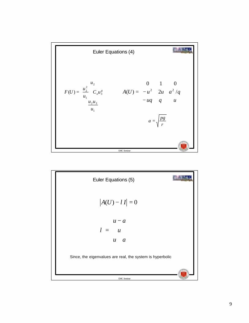
EulerEuler Equations (4)Equations (4)
+=
1
32
31
22
2
)(
uuu
uCuu
u
UF oγ
−−=⇒
uuauuUA
θθθ/2
010)( 22
ργp
a =
EMC SeminarEMC Seminar
EulerEuler Equations (5)Equations (5)
Since, the eigenvalues are real, the system is hyperbolic
0)( =− IUA λ
+
−=
auu
auλ
10
EMC SeminarEMC Seminar
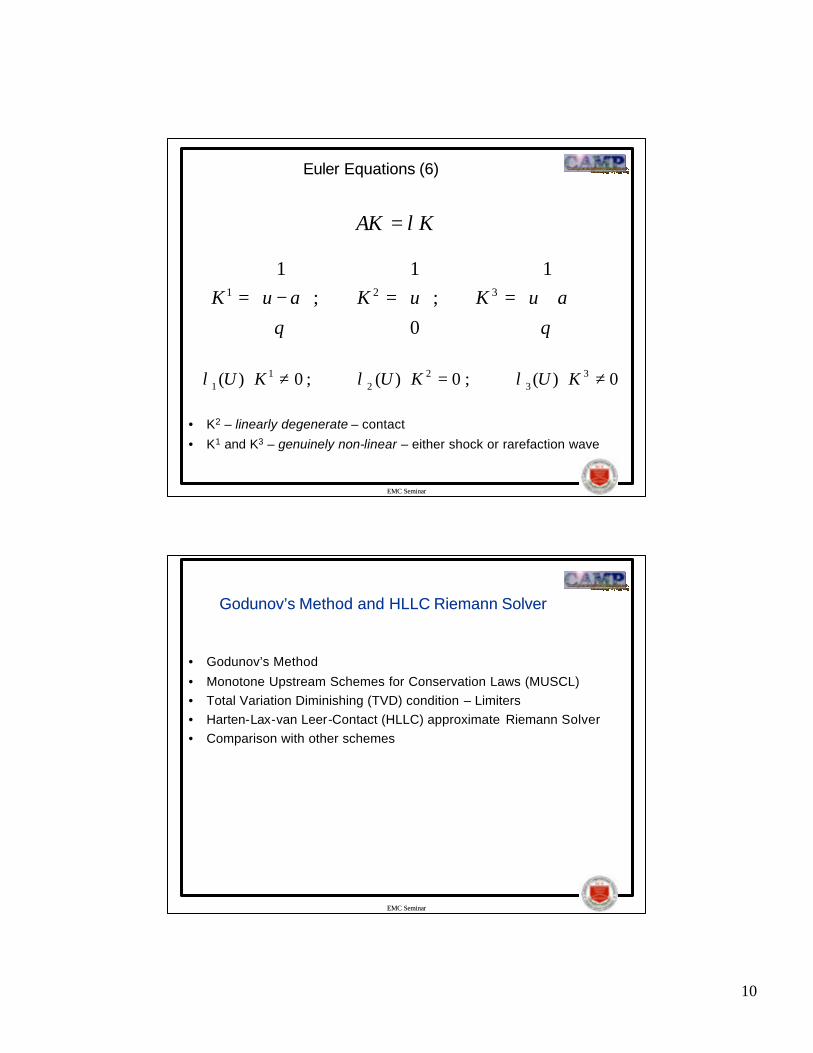
EulerEuler Equations (6)Equations (6)
• K2 – linearly degenerate – contact
• K1 and K3 – genuinely non-linear – either shock or rarefaction wave
KAK λ=
+=
=
−=
θθ
auKuKauK1
;
0
1;
1321
0)(;0)(;0)( 33
22
11 ≠⋅∇=⋅∇≠⋅∇ KUKUKU λλλ
EMC SeminarEMC Seminar
Godunov’sGodunov’s Method and HLLC Method and HLLC Riemann Riemann SolverSolver
• Godunov’s Method
• Monotone Upstream Schemes for Conservation Laws (MUSCL)• Total Variation Diminishing (TVD) condition – Limiters• Harten-Lax-van Leer-Contact (HLLC) approximate Riemann Solver• Comparison with other schemes

11
EMC SeminarEMC Seminar
Godunov’s Godunov’s MethodMethod
+
∆∆
+=+−
+
21
21
1
ii
ni
ni FF
xt
UU
))0((21
21
++=
iiUFF
EMC SeminarEMC Seminar
MUSCL (van Leer) MUSCL (van Leer) –– TVD (TVD (HartenHarten, , SpekreijseSpekreijse))
• No new local extrema in ‘x’ may be created
• The value of a local minima increases• The value of a local maxima decreases
)()( iedgeiiedge xxuiuu −⋅∇⋅+= φ
),max(),min( 1211 +++ ≤≤ iiiii uuuuu
12
EMC SeminarEMC Seminar
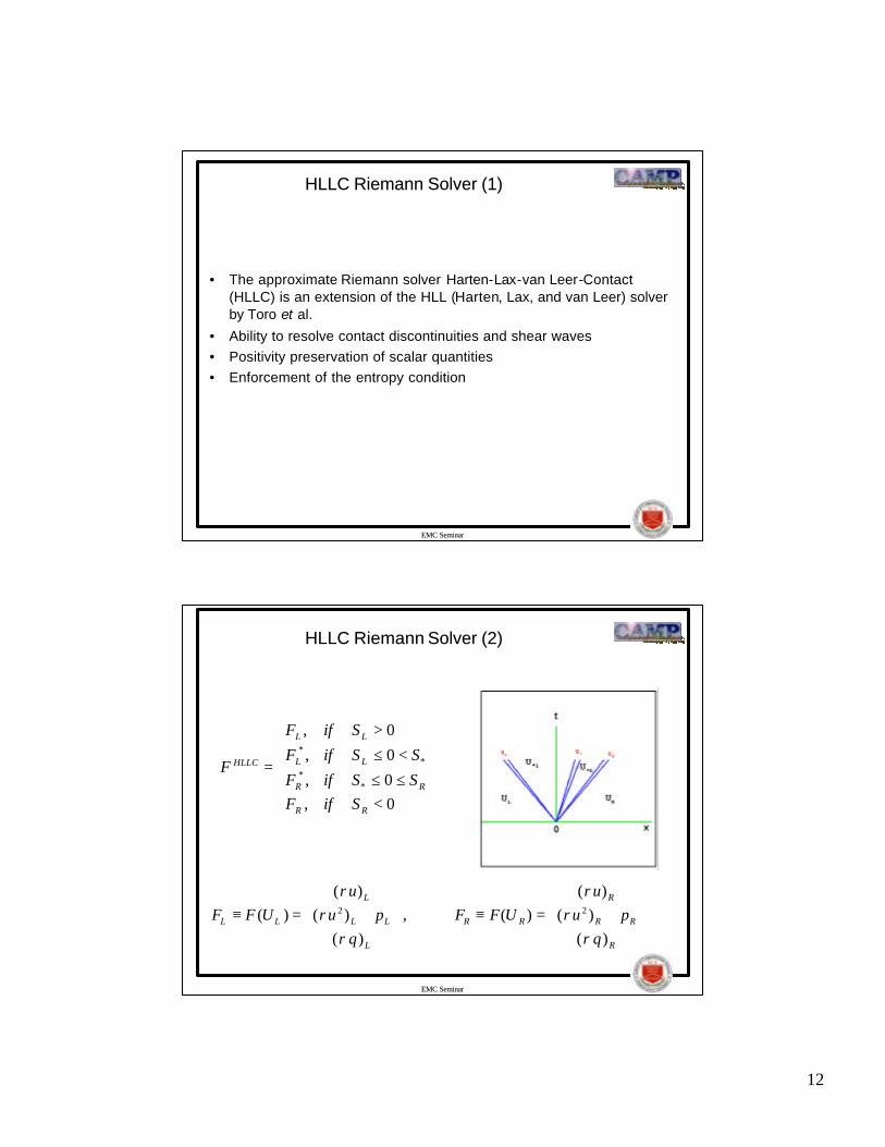
HLLC HLLC Riemann Riemann Solver (1)Solver (1)
• The approximate Riemann solver Harten-Lax-van Leer-Contact (HLLC) is an extension of the HLL (Harten, Lax, and van Leer) solver by Toro et al.
• Ability to resolve contact discontinuities and shear waves• Positivity preservation of scalar quantities• Enforcement of the entropy condition
EMC SeminarEMC Seminar
HLLC HLLC RiemannRiemann Solver (2)Solver (2)
<≤≤<≤
>
=
0,0,
0,
0,
**
**
RR
RR
LL
LL
HLLC
SifFSSifF
SSifF
SifF
F
+=≡
+=≡
R
RR
R
RR
L
LL
L
LL puu
UFFpuu
UFF)(
)()(
)(,)(
)()(
)( 22
ρθρ
ρ
ρθρ
ρ
13
EMC SeminarEMC Seminar
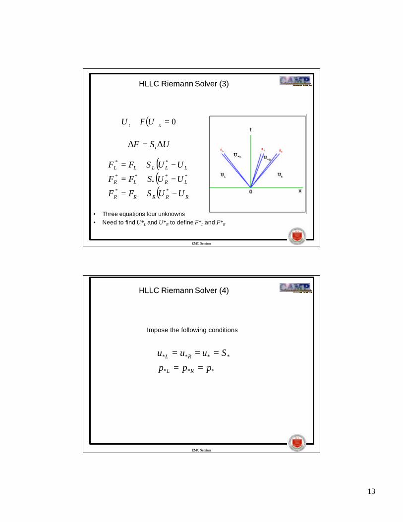
HLLC HLLC RiemannRiemann Solver (3)Solver (3)
• Three equations four unknowns• Need to find U*L and U*R to define F*L and F*R
( ) 0=+ xt UFU
USF i ∆=∆
( )( )( )RRRRR
LRLR
LLLLL
UUSFF
UUSFF
UUSFF
−+=
−+=
−+=
**
***
**
**
EMC SeminarEMC Seminar
HLLC HLLC RiemannRiemann Solver (4)Solver (4)
Impose the following conditions
***
****
ppp
Suuu
RL
RL
==
===

14
EMC SeminarEMC Seminar
HLLC HLLC Riemann Riemann Solver (5)Solver (5)
+=≡*
*
***
**
**
)()()(
L
LL
L
LL
SpuS
S
UFFρθ
ρρ
−−+−
−
−=
=
LLL
LLLLL
LLL
LL
L
L
L
uSppuuS
uS
SSuU
))(()())((
)(1
)()( *
**
*
*
*
ρθρ
ρ
ρθρρ
EMC SeminarEMC Seminar
HLLC HLLC Riemann Riemann Solver (6)Solver (6)
+=≡*
*
***
**
**
)()()(
R
RR
R
RR
SpuS
SUFF
ρθρ
ρ
−−+−
−
−=
=
RRR
RRRRR
RRR
RR
R
R
R
uSppuuS
uS
SSuU
))(()())((
)(1
)()( *
**
*
*
*
ρθρ
ρ
ρθρρ

15
EMC SeminarEMC Seminar
HLLC HLLC Riemann Riemann Solver (7)Solver (7)
))((),)(( **
**
RRRRRRLLLLLL uSuSppuSuSpp −−+=−−+= ρρ
)()()()(
*LLLRRR
RLLLLLRRRR
uSuSppuSuuSu
S−−−
−+−−−=
ρρρρ
RRRLLL auSauS +=−=
EMC SeminarEMC Seminar
ComparisonComparison
Mendez-Nunez and Caroll , Mon. Wea. Rev., 121, 565-578.
Leapfrog
Smolarkiewicz
MacCormack

16
EMC SeminarEMC Seminar
Comparison (cont’d)Comparison (cont’d)
Mendez-Nunez and Caroll , Mon. Wea. Rev ., 121, 565-578.
Leapfrog
Smolarkiewicz
MacCormack
EMC SeminarEMC Seminar
Comparison (cont’d)Comparison (cont’d)
Mendez-Nunez and Caroll , Mon. Wea. Rev., 121, 565-578.
MacCormack
Smolarkiewicz
Leapfrog

17
EMC SeminarEMC Seminar
Comparison (cont’d)Comparison (cont’d)
EMC SeminarEMC Seminar
SmagorinskySmagorinskySchemeScheme
Deformation is related to the eddy viscosity (Smagorinsky-Lilly):
<−∆
=otherwise
RiifRiDefc
Km
0
25.0)1(2)( 5.0
2
∑∑=j
iji
DDef 22
21
2
∂∂
∂∂
=
yu
ygRi
θ
θ
222
∂∂
+∂∂
+
∂∂
−∂∂
=xv
yu
yv
xu
Def

18
EMC SeminarEMC Seminar
RungeRunge--Kutta Kutta Time MarchingTime Marching
)4(1
)3(4
)0()4(
)2(3
)0()3(
)1(2
)0()2(
)0(1
)0()1(
)0(
ini
iii
iii
iii
iii
nii
UU
tRUU
tRUU
tRUU
tRUU
UU
=
∆−=
∆−=
∆−=
∆−=
=
+
α
α
α
α
auabsx
CFLt+
∆⋅=∆
)(
EMC SeminarEMC Seminar
Implementation on Unstructured MeshesImplementation on Unstructured Meshes
• Overview
• Data Structures• Calculation of Convective Fluxes• Reconstruction• Limiters• Boundary Conditions

19
EMC SeminarEMC Seminar
Implementation on Unstructured Mesh (1)Implementation on Unstructured Mesh (1)
• OMEGA data structures (Lottati and Eidelman, Bacon et al.)
• Higher-order spatial accuracy from either Green-Gauss or Linear-Least Squares reconstruction
• TVD condition enforced via slope limiters (Barth-Jesperson or van Leer)
• Limiting performed on conserved variables• Option of 2 or 4-stage explicit Runge-Kutta Time marching
scheme (Jameson-Schmidt-Turkel)• Diffusion operator calculated using pseudo-Laplacians (Holmes
and Connell)• Subgrid-scale diffusion from Smagorinsky scheme
• Edge-based solver
EMC SeminarEMC Seminar
Implementation on Unstructured Mesh (2)Implementation on Unstructured Mesh (2)
Cell-centered control volumes
Cell Connectivity:Cell Connectivity:jelem(cell,1)=iv1 (node1)jelem(cell,2)=iv2 (node2)jelem(cell,3)=iv3 (node3)jelem(cell,4)=ie1 (edge1)jelem(cell,5)=ie2 (edge2)jelem(cell,6)=ie3 (edge3)
Edge Connectivity:Edge Connectivity:jedge(edge,1)=iv1 (node1)jedge(edge,2)=iv1 (node2)jedge(edge,3)=ic1 (cell1)jedge(edge,4)=ic2 (cell2)jedge(edge,5)= edge type

20
EMC SeminarEMC Seminar
Implementation on Unstructured Mesh (3)Implementation on Unstructured Mesh (3)
∫∫ΓΩ
Γ−=Ω dnGFdUdtd r
).,(
0),( =⋅+ ∑ sGFdt
duV
faces
cellcell
Ω
Γ
EMC SeminarEMC Seminar
Implementation on Unstructured Mesh (4)Implementation on Unstructured Mesh (4)
• Reconstruction via either Green-Gauss or Linear Least-Squares
• Option of Barth-Jesperson and van Leer limiters
)()( iedgeiiedge xxuiuu −⋅∇⋅+= φ
∫∫ΓΩ
Γ=Ω∇ dnudur
.

21
EMC SeminarEMC Seminar
Implementation on Unstructured Mesh (5)Implementation on Unstructured Mesh (5)
),(minminioNij uuu
j∈= ),(maxmax
ioNij uuuj∈
=
maxmin ),( joj uyxuu ≤≤
=−
<−−
−
>−−
−
=
01
0),1min(
0),1min(
min
max
oLi
oLi
oLi
oj
oLi
oLi
oj
face
uuif
uuifuu
uu
uuifuu
uu
L
EMC SeminarEMC Seminar
Scalar Advection EquationScalar Advection Equation
• Rotating Cone Test (convergence)
• Smolarkiewicz’s Deformational Flow (stability)• Doswell’s Frontogenesis (accuracy/convergence)• Solution-Adaptation Demonstration

22
EMC SeminarEMC Seminar
Rotating Cone TestsRotating Cone Tests
EMC SeminarEMC Seminar
Rotating Cone TestsRotating Cone Tests
initial condition (left), initial condition (left), godunov godunov (center) and (center) and musclmuscl (right)(right)

23
EMC SeminarEMC Seminar
Smolarkiewicz’sSmolarkiewicz’s Deformational FlowDeformational Flow
• The flow field consists of sets of symmetrical vortices.• A = 8 and L = 100 units (size of the domain was 100x100 units) • In the words of Smolarkiewicz, “the deformational flow test is a
convenient tool for studying a solution’s accuracy on the resolved scales and for addressing questions of nonlinear instability due to the existence of unresolved scales ”
( ) ( )kykxAky
yxu sinsin),( =∂∂
=ψ
( ) ( )kykxAkx
yxv coscos),( =∂∂−= ψ
Lk
π4=
EMC SeminarEMC Seminar
Smolarkiewicz’s Smolarkiewicz’s Deformational FlowDeformational Flow

24
EMC SeminarEMC Seminar
Smolarkiewicz’s Smolarkiewicz’s Deformational FlowDeformational Flow
EMC SeminarEMC Seminar
Doswell’s FrontogenesisDoswell’s Frontogenesis
• Doswell’s idealized model describes the interaction of a nondivergent vortex with an initially straight frontal zone
• r is the distance from any given point to the origin of the coordinate system • fmax = 0.385 is the maximum tangential velocity• The solution domain was bounded within x:[-4,4] and y:[-4,4]• simulation was run for t = 4 units
maxmax
),(;),(ff
rxyxv
ff
ryyxu tt =−=
)(cosh)tanh(
2 rrf t =
⋅−⋅−= )sin(
2)cos(
2tanh),,( tfxtfytyxq

25
EMC SeminarEMC Seminar
Doswell’s FrontogenesisDoswell’s Frontogenesis
EMC SeminarEMC Seminar
Doswell’s FrontogenesisDoswell’s Frontogenesis

26
EMC SeminarEMC Seminar
Doswell’s FrontogenesisDoswell’s Frontogenesis
• Three cases:– regular mesh (with smoothing)– distorted mesh (no smoothing)– mesh with right angle triangles
• Comparison of reconstruction techniques• Accuracy
nelem
yxqyxqerror
nelem
exactsimulated∑ −= 1
2),(),(
EMC SeminarEMC Seminar
Doswell’s FrontogenesisDoswell’s Frontogenesis
Mesh 1
Mesh 2
Mesh 3
27
EMC SeminarEMC Seminar
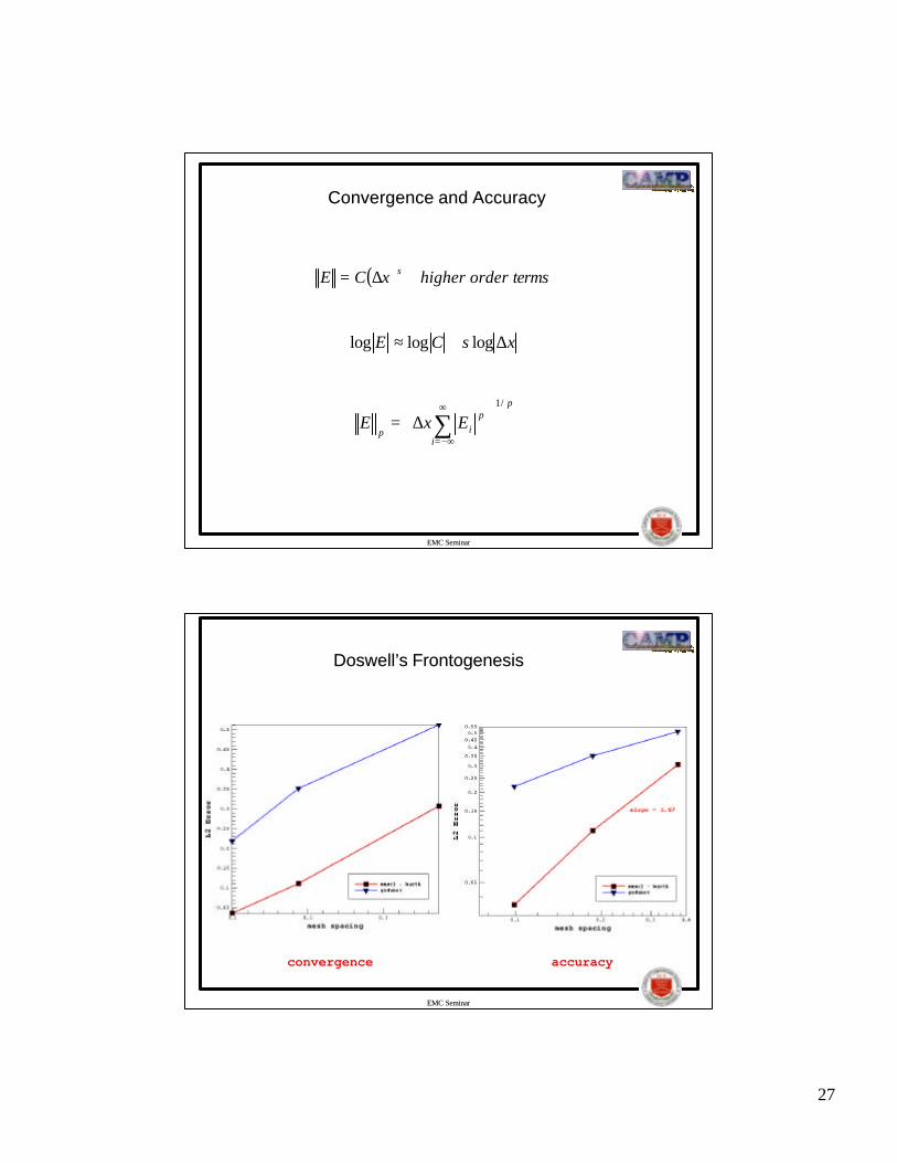
Convergence and AccuracyConvergence and Accuracy
p
i
pip
ExE/1
∆= ∑
∞
−∞=
( ) termsorderhigherxCE s +∆=
xsCE ∆+≈ logloglog
EMC SeminarEMC Seminar
Doswell’s FrontogenesisDoswell’s Frontogenesis
convergence accuracy
28
EMC SeminarEMC Seminar
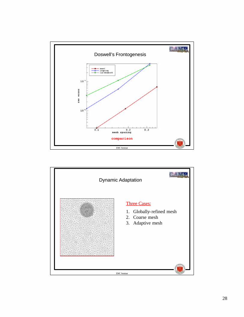
Doswell’s FrontogenesisDoswell’s Frontogenesis
comparison
EMC SeminarEMC Seminar
Dynamic AdaptationDynamic Adaptation
Three Cases:Three Cases:
1. Globally-refined mesh2. Coarse mesh3. Adaptive mesh
29
EMC SeminarEMC Seminar
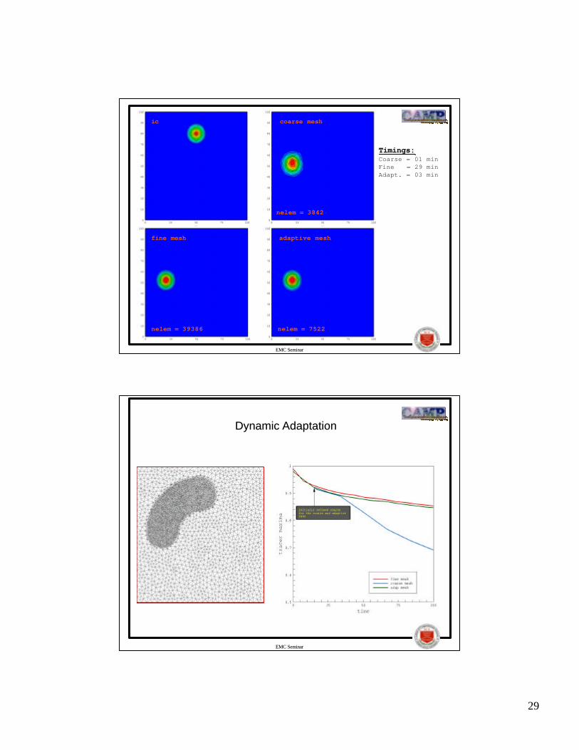
fine mesh
coarse mesh
adaptive mesh
ic
Timings:Timings:Coarse = 01 minFine = 29 minAdapt. = 03 min
nelem = 39386 nelem = 7522
nelem = 3842
EMC SeminarEMC Seminar
Dynamic AdaptationDynamic Adaptation

30
EMC SeminarEMC Seminar
Sod Shock TubeSod Shock Tube
EMC SeminarEMC Seminar
Sod Shock TubeSod Shock Tube

31
EMC SeminarEMC Seminar
Urban Street CanyonUrban Street Canyon
• X [-750 : 750 m]
• Y [0 : 800 m]• Edge lengths [2.16-12.14 m]• nelem = 66585• Stable Atmosphere• Hydrostatic balance initially• Logarithmic flow profile• u* = 0.2 m/s• y0 = 15 cm• tmax = 21.8 sec
=
oyy
ku
yu ln)( *
EMC SeminarEMC Seminar
Urban Street CanyonUrban Street Canyon
pressurepressure thetatheta
uu--velocityvelocity meshmesh

32
EMC SeminarEMC Seminar
Urban Street CanyonUrban Street Canyon
EMC SeminarEMC Seminar
Urban Street CanyonUrban Street Canyon

33
EMC SeminarEMC Seminar
Convection in Neutral AtmosphereConvection in Neutral Atmosphere
• 1km X 1km Domain
• Edge lengths from 3.5m to 12.4m• Atmosphere at 300K• Hydrostatic balance initially• Bubble radius = 100m• Bubble center height = 120m• Bubble over-temperature = 6.6K
• Linear temperature profile within the warm bubble• U = 0 and V = 0• Fields initialized on a structured grid and then interpolated to the
unstructured mesh
EMC SeminarEMC Seminar
Convection in Neutral AtmosphereConvection in Neutral Atmosphere
initial conditions

34
EMC SeminarEMC Seminar
Convection in Neutral AtmosphereConvection in Neutral Atmosphere
godunov muscl
EMC SeminarEMC Seminar
Convection in Neutral AtmosphereConvection in Neutral Atmosphere
godunov muscl

35
EMC SeminarEMC Seminar
Convection in Neutral AtmosphereConvection in Neutral Atmosphere
godunov muscl
EMC SeminarEMC Seminar
Convection in Neutral AtmosphereConvection in Neutral Atmosphere
Conservation of Mass and Energy-density (Simulation time = 360 s)
Scheme Einitial Efinal Minitial Mfinal Iterations
Godunov 334486112 334486112 1114695.5 1114695.6 155,000
MUSCL 334486112 334486114 1114691.6 1114691.7 248,000

36
EMC SeminarEMC Seminar
KelvinKelvin--HelmholtzHelmholtz InstabilityInstability
Often occurs in the atmosphere.Sometimes can be observed in billow clouds.Thought to be a major trigger of clear air turbulence (CAT).
“La “La Nuit EtoileeNuit Etoilee””Vincent van Vincent van GoghGogh
2
∂∂
∂∂
=
yu
ygRi
θ
θ
EMC SeminarEMC Seminar
KelvinKelvin--HelmholtzHelmholtz InstabilityInstability

37
EMC SeminarEMC Seminar
KelvinKelvin--HelmholtzHelmholtz InstabilityInstability
EMC SeminarEMC Seminar
KelvinKelvin--HelmholtzHelmholtz InstabilityInstability

38
EMC SeminarEMC Seminar
ConclusionsConclusions
• A high-resolution Godunov-type scheme implemented on unstructured meshes for simulating atmospheric flows
• Conservative Finite Volume discretization capable of resolving flows with sharp gradients
• Higher-order spatial accuracy via MUSCL (van Leer)• Explicit Runge-Kutta time marching• TVD condition enforced via slope limiters• Exhibits minimal phase errors and numerical diffusion• Subgrid-scale diffusion (Smagorinsky closure) added as source term
• Validated against idealized benchmark cases
EMC SeminarEMC Seminar
Future WorkFuture Work
• Implicit time-marching (Sharov, Luo et al., Batten et al.)• Examine the role of different types of limiters (Hubbard)• Extend to three dimensions (prismatic elements)• Solution-adaptive techniques (Löhner)• Efficient data structures (Löhner)• Quadratic reconstruction schemes (Mitchell)• Test other turbulence schemes (Mellor-Yamada, Germano-Lilly)• Add more physics (radiation/microphysics)• Code optimization – Parallelization (MPI)