The relationship between FST and the frequency of the most frequent allele

Mattias Jakobsson∗

Department of Evolutionary Biology and Science for Life Laboratory, Uppsala University

Michael D. EdgeDepartment of Biology, Stanford University

Noah A. RosenbergDepartment of Biology, Stanford University

October 24, 2012

FST is frequently used as a summary of genetic differentiation among groups. It has been suggested that FST depends on the allele frequenciesat a locus, as it exhibits a variety of peculiar properties related to genetic diversity: higher values for biallelic single-nucleotide polymorphisms(SNPs) than for multiallelic microsatellites, low values among high-diversity populations viewed as substantially distinct, and low values forpopulations that differ primarily in their profiles of rare alleles. A full mathematical understanding of the dependence of FST on allele frequencies,however, has been elusive. Here, we examine the relationship between FST and the frequency of the most frequent allele, demonstrating thatthe range of values that FST can take is restricted considerably by the allele frequency distribution. For a two-population model, we derive strictbounds on FST as a function of the frequency M of the allele with highest mean frequency between the pair of populations. Using these bounds,we show that for a value of M chosen uniformly between 0 and 1 at a multiallelic locus whose number of alleles is left unspecified, the meanmaximum FST is ∼0.3585. Further, FST is restricted to values much less than 1 when M is low or high, and the contribution to the maximum FST

made by the most frequent allele is on average ∼0.4485. Using bounds on homozygosity that we have previously derived as functions of M , wedescribe strict bounds on FST in terms of the homozygosity of the total population, finding that the mean maximum FST given this homozygosity is1− ln 2 ≈ 0.3069. Our results provide a conceptual basis for understanding the dependence of FST on allele frequencies and genetic diversity, andfor interpreting the roles of these quantities in computations of FST from population-genetic data. Further, our analysis suggests that many unusualobservations of FST , including the relatively low FST values in high-diversity human populations from Africa and the relatively low estimatesof FST for microsatellites compared to SNPs, can be understood not as biological phenomena associated with different groups of populations orclasses of markers but rather as consequences of the intrinsic mathematical dependence of FST on the properties of allele frequency distributions.

Differentiation among groups is one of the fundamental sub-jects of the field of population genetics. Comparisons of thelevel of variation among subpopulations with the level of vari-ation in the total population have been employed frequently inpopulation-genetic theory, in statistical methods for data analy-sis, and in empirical studies of distributions of genetic variation.Wright’s (WRIGHT 1951) fixation indices, and FST in particu-lar, have been central to this effort.

Wright’s FST was originally defined as the correlation be-tween two randomly sampled gametes from the same subpop-ulation when the correlation of two randomly sampled ga-metes from the total population is set to zero. Several defi-nitions of FST or FST -like quantities are now available, re-lying on a variety of different conceptual formulations butall measuring some aspect of population differentiation (e.g.CHARLESWORTH 1998; HOLSINGER and WEIR 2009). Manyauthors have claimed that one or another formulation of FST isaffected by levels of genetic diversity or by allele frequencies,either because the range of FST is restricted by these quanti-

ties or because these quantities affect the degree to which FST

reflects population differentiation (e.g. CHARLESWORTH 1998;NAGYLAKI 1998; HEDRICK 1999, 2005; LONG and KITTLES2003; RYMAN and LEIMAR 2008; JOST 2008; LONG 2009;MEIRMANS and HEDRICK 2011). For example, NAGYLAKI(1998) and HEDRICK (1999) argued that measures of FST maybe poor measures of genetic differentiation when the level ofdiversity is high. CHARLESWORTH (1998) suggested that FST

can be inflated when diversity is low, arguing that FST mightnot be appropriate for comparing loci with substantially differ-ent levels of variation. In a provocative recent article, JOST(2008) has used the diversity dependence of forms of FST toquestion their utility as differentiation measures at all.

One definition that is convenient for mathematical assess-ment of the relationship of an FST -like quantity and allele fre-quencies is the quantity labeled GST by NEI (1973), which for agiven locus measures the difference between the heterozygosityof the total (pooled) population, hT , and the mean heterozygos-ity across subpopulations, hS , divided by the heterozygosity of

∗Corresponding author: Uppsala University, Norbyvägen 18D, SE-752 36, Uppsala, Sweden. Email: mattias.jakobsson@ebc.uu.se

1

Genetics: Advance Online Publication, published on November 19, 2012 as 10.1534/genetics.112.144758

Copyright 2012.

the total population:

GST =hT − hS

hT. (1)

In terms of the homozygosity of the total population, HT =1 − hT , and the mean homozygosity across subpopulations,HS = 1− hS , we can write

GST =HS −HT

1−HT. (2)

The WAHLUND (1928) principle guarantees that HS ≥ HT ,and therefore, because HS ≤ 1 and for a polymorphic locuswith finitely many alleles, 0 < HT < 1, GST lies in the inter-val [0,1].

Using GST for their definition of FST , HEDRICK (1999,2005) and LONG and KITTLES (2003) pointed out that becausehT < 1, FST cannot exceed the mean homozygosity acrosssubpopulations, HS :

FST = 1− hS/hT < 1− hS = HS . (3)

HEDRICK (2005) obtained this result by considering a set of Kequal-sized subpopulations, in which each allele is private to asingle subpopulation. In the limit as K → ∞, a stronger upperbound on FST as a function of HS and K reduces to eq. 3 (seealso JIN and CHAKRABORTY (1995) and LONG and KITTLES(2003)).

While HEDRICK (1999, 2005) and LONG and KITTLES(2003) have clarified the relationship between FST and themean homozygosity HS across subpopulations, their ap-proaches do not easily illuminate the connection between FST

and allele frequencies themselves. A formal understandingof the relationship between FST and allele frequencies wouldmake it possible to more fully understand the behavior of FST

in situations where markers of interest differ substantially in al-lele frequencies or levels of genetic diversity. Our recent workon the relationship between homozygosity and the frequency ofthe most frequent allele (ROSENBERG and JAKOBSSON 2008;REDDY and ROSENBERG 2012) provides a mathematical ap-proach for formal investigation of bounds on population-geneticstatistics in terms of allele frequencies. In this paper, we there-fore seek to thoroughly examine the dependence of FST on al-lele frequencies by investigating the upper bound on FST interms of the frequency M of the most frequent allele across apair of populations. We derive bounds on FST given the fre-quency of the the most frequent allele and bounds on the fre-quency of the most frequent allele given FST . We consider lociwith arbitrarily many alleles in a pair of subpopulations. Usingtheory for the bounds on homozygosity given the frequency ofthe most frequent allele, we obtain strict bounds on FST giventhe homozygosity of the total population. Our analysis clarifiesthe relationships among FST , allele frequencies, and homozy-gosity, providing explanations for peculiar observations of FST

that can be attributed to allele-frequency dependence.

MODEL

We examine a polymorphic locus with at least two alleles in asetting with K subpopulations that contribute equally to a to-tal population. Denote the number of distinct alleles by I , thefrequency of allele i in population k by pki, and the mean fre-quency of allele i across populations by p̄i =

1K

∑Kk=1 pki. We

primarily report our results in terms of homozygosities, whichcan be easily transformed into heterozygosities.

We consider FST formulated as a property of nonnegativenumbers between 0 and 1 such that within populations, the al-lele frequencies sum to 1 (

∑Ii=1 pki = 1 for each k). This

formulation is the same as the formulation of Nei’s GST , whichwe hereafter denote by F . We have (NEI 1973):

F =hT − hS

hT=

HS −HT

1−HT

where

HT =I∑

i=1

p̄2i =I∑

i=1

(1

K

K∑k=1

pki

)2

and

HS =1

K

K∑k=1

( I∑i=1

p2ki

)=

1

K

K∑k=1

I∑i=1

p2ki.

The assumption that the locus is polymorphic guarantees thatHT < 1. The assumption that I , the number of distinct alleles atthe locus, is finite guarantees that HT > 0 (and hence HS > 0because HS ≥ HT ). Thus, 0 < HT < 1 and 0 < HS ≤ 1.

We assume that all allele frequencies are the parametric al-lele frequencies of the population under consideration. Thus,the frequency of an allele is the probability of drawing the al-lele from the parametric frequency distribution; homozygosityis then the probability that two independent random draws carrythe same allelic type, and heterozygosity is the probability thattwo independent random draws carry different allelic types. Weemphasize that in our formulation, F , HT , and HS are func-tions of the parametric allele frequencies, and our interest is inthe properties of these functions and their relationships with theallele frequencies; we do not investigate their estimation fromdata, nor do we consider how evolutionary models affect theunderlying allele frequencies involved in their computation.

Two populations: We focus on the case of K = 2 subpop-ulations. In this case, the allele frequencies are denoted p1i forpopulation 1 and p2i for population 2. For each i from 1 to I , letσi = p1i+p2i be the sum across populations of the frequency ofallele i. Each σi lies in (0, 2), and the number of alleles I countsonly those alleles with σi > 0. We denote p̄i = σi/2. Withoutloss of generality, we place the alleles in decreasing order, suchthat σ1 ≥ σ2 ≥ ... ≥ σI . We denote the frequency of the mostfrequent allele in the total pooled population by M = σ1/2,and we find it convenient to express some results in terms of σ1

and others in terms of M . Because∑I

i=1 σi = 2 and each σi ispositive, we have 1/I ≤ M < 1.

2

Let δi = |p1i − p2i| be the absolute difference between p1iand p2i. We can write the homozygosity of the total populationas

HT =I∑

i=1

p̄2i =1

4

I∑i=1

σ2i ,

and the mean homozygosity across subpopulations as

HS =1

2

2∑k=1

I∑i=1

p2ki =1

2

I∑i=1

(p21i + p22i).

We then have (BOCA and ROSENBERG 2011)

F =

∑Ii=1 δ

2i

4−∑I

i=1 σ2i

. (4)

In other words, F can be computed solely using the allele fre-quency sums and differences between the two populations.

BOUNDS ON F

Our goal is to study the relationship between F and M in thegeneral case of I alleles in two populations. For convenience,we write F as a function of σ1, keeping in mind that σ1/2 = M ,and we begin by considering the special case in which I = 2.

Bounds on F for two alleles: This case has two alleles,with frequencies p11 and p12 in population 1, and p21 and p22in population 2 (Table 1). The frequency of the second allele isp12 = 1− p11 in population 1 and p22 = 1− p21 in population2. Using eq. 4, we have a simple expression for F (WEIR 1996;ROSENBERG et al. 2003):

F =δ21 + [(1− p11)− (1− p21)]

2

4− σ21 − [(1− p11) + (1− p21)]2

=δ21

σ1(2− σ1). (5)

We determine the upper and lower bounds of F in termsof the frequency of the most frequent allele M = σ1/2. Be-cause the alleles are arranged to satisfy σ1 ≥ σ2 and becauseσ1 + σ2 = 2, σ1 must lie in [1, 2). For the lower bound onF as a function of σ1, we note that if allele 1 has the samefrequency in both populations, then p11 = p21 = σ1/2. Thefrequency of allele 2 will also be the same in the two popula-tions, p12 = p22 = 1 − σ1/2, and δ1 and δ2 will both equalzero. For these allele frequencies, we see that HS = HT , and itis clear from eq. 5 that F (σ1) ≥ 0 for all values of σ1 in [1, 2),with equality if and only if p11 = p21 = σ1/2.

Table 1: Notation for two alleles in two populations.Allele

Population 1 2 Sum1 p11 p12 12 p21 p22 1

Sum σ1 σ2 2Absolute difference δ1 δ2 -

Frequency of the most frequent allele (M = σ1 2)

F

0.5 0.6 0.7 0.8 0.9 10

0.1

0.2

0.3

0.4

0.5

0.6

0.7

0.8

0.9

1

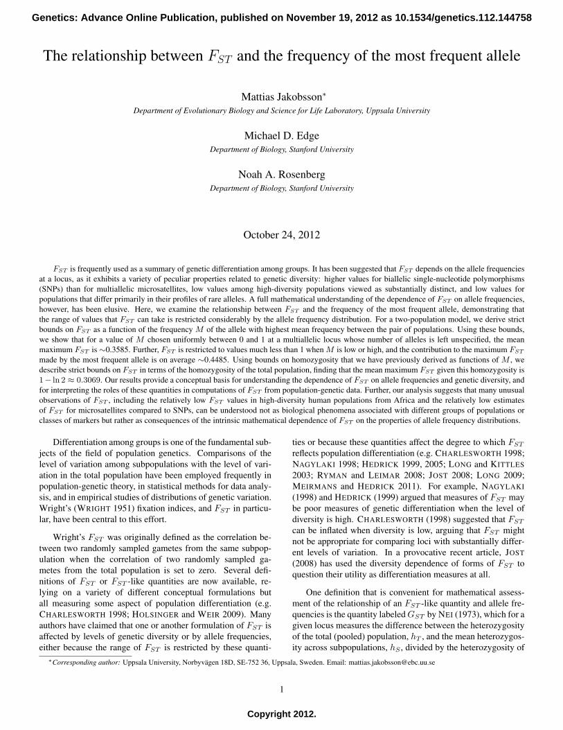
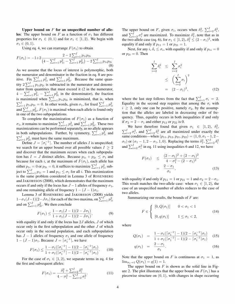
Figure 1: The upper bound on F as a function of the frequency Mof the most frequent allele, for the two-allele case. The upper bound iscomputed from eq. 7. The lower bound on F is 0 for all values of M .

For the upper bound, we first note that because δ1 = 2p11−σ1 when p11 ≥ p21 and δ1 = 2p21 − σ1 when p21 ≥ p11,

δ21 ≤ (2− σ1)2, (6)

with equality if and only if p11 = 1 or p21 = 1. Using eqs. 5and 6, we have

F (σ1) ≤(2− σ1)

2

σ1(2− σ1)=

2− σ1

σ1.

Thus, the upper bound on F as a function of σ1 is achievedwhen the allele frequencies of the two populations differ asmuch as possible, that is, when (p11, p21) = (1, σ1 − 1) or(p11, p21) = (σ1 − 1, 1). The bounds on F are

F ∈[0,

2− σ1

σ1

]. (7)

Figure 1 shows the upper bound as a function of the most fre-quent allele, illustrating a monotonic decline from q(1/2) = 1to q(1) = 0.

Lower bound on F for an unspecified number of alleles:For any number of alleles I and any set of σi, by noting that thedenominator of F in eq. 4 is positive and that the numerator is∑I

i=1 δ2i ≥ 0, we see that eq. 4 takes the value of zero if and

only if for each i, p1i = p2i = σi/2. Thus, the lower boundon F as a function of σ1 is achieved when the allele frequenciesare the same in both populations for all I alleles. Thus, F = 0is attainable for any value of σ1 in (0, 2).

3

Upper bound on F for an unspecified number of alle-les: The upper bound on F as a function of σ1 has differentproperties for σ1 ∈ (0, 1) and for σ1 ∈ [1, 2). We begin withσ1 ∈ (0, 1).

Using eq. 4, we can rearrange F (σ1) to obtain

F (σ1) = −1+22− 2

∑Ii=1 p1ip2i(

4−∑I

i=1 p21i −

∑Ii=1 p

22i

)− 2

∑Ii=1 p1ip2i

.

(8)As we assume that the locus of interest is polymorphic, boththe numerator and denominator in the fraction in eq. 8 are pos-itive. Fix

∑Ii=1 p

21i and

∑Ii=1 p

22i. Because the same quan-

tity 2∑I

i=1 p1ip2i is subtracted in the numerator and denomi-nator from quantities that must exceed it (2 in the numerator,4 −

∑Ii=1 p

21i −

∑Ii=1 p

22i in the denominator), the fraction

is maximized when∑I

i=1 p1ip2i is minimized, that is, when∑Ii=1 p1ip2i = 0. In other words, given σ1, for fixed

∑Ii=1 p

21i

and∑I

i=1 p22i, F (σ1) is maximal when each allele is found only

in one of the two subpopulations.To complete the maximization of F (σ1) as a function of

σ1, it remains to maximize∑I

i=1 p21i and

∑Ii=1 p

22i. These two

maximizations can be performed separately, as no allele appearsin both subpopulations. Further, by symmetry,

∑Ii=1 p

21i and∑I

i=1 p22i must have the same maximum.

Define J = ⌈σ−11 ⌉. The number of alleles I is unspecified;

we search for an upper bound over all possible values I ≥ 2and discover that the maximum occurs when each subpopula-tion has I = J distinct alleles. Because p1i + p2i ≤ σ1 andbecause for each i, at the maximum of F (σ1), each allele haseither p1i = 0 or p2i = 0, it suffices to maximize

∑Ii=1 p

21i sub-

ject to∑I

i=1 p1i = 1 and p1i ≤ σ1 for all i. This maximizationis the same problem considered in Lemma 3 of ROSENBERGand JAKOBSSON (2008), which demonstrates that the maximumoccurs if and only if the locus has J −1 alleles of frequency σ1,and one remaining allele of frequency 1− (J − 1)σ1.

Lemma 3 of ROSENBERG and JAKOBSSON (2008) yields1−σ1(J−1)(2−Jσ1) for each of the two maxima, on

∑Ii=1 p

21i

and on∑I

i=1 p22i. We then conclude

F (σ1) ≤1− σ1(J − 1)(2− Jσ1)

1 + σ1(J − 1)(2− Jσ1), (9)

with equality if and only if the locus has 2J alleles, J of whichoccur only in the first subpopulation and the other J of whichoccur only in the second population, and each subpopulationhas J − 1 alleles of frequency σ1 and one allele of frequency1− (J − 1)σ1. Because J = ⌈σ−1

1 ⌉, we have

F (σ1) ≤1− σ1(⌈σ−1

1 ⌉ − 1)(2− ⌈σ−11 ⌉σ1)

1 + σ1(⌈σ−11 ⌉ − 1)(2− ⌈σ−1

1 ⌉σ1). (10)

For the case of σ1 ∈ [1, 2), we separate terms in eq. 4 forthe first and subsequent alleles:

F (σ1) =δ21 +

∑Ii=2 δ

2i

4− σ21 −

∑Ii=2 σ

2i

. (11)

The upper bound on F , given σ1, occurs when δ21 ,∑I

i=2 δ2i ,

and∑I

i=2 σ2i are maximized. To maximize δ21 , note that as in

the two-allele case (eq. 6), for σ1 ∈ [1, 2), δ21 ≤ (2−σ1)2, with

equality if and only if p11 = 1 or p21 = 1.Next, for any i, δi ≤ σi, with equality if and only if p1i = 0

or p2i = 0. Then

I∑i=2

δ2i ≤I∑

i=2

σ2i

≤( I∑

i=2

σi

)2

= (2− σ1)2, (12)

where the last step follows from the fact that∑I

i=1 σi = 2.Equality in the second step requires that among the σi withi ≥ 2, only one can be positive, namely σ2, by the assump-tion that the alleles are labeled in decreasing order of fre-quency. Thus, equality occurs in both inequalities if and onlyif σ2 = 2− σ1 and either p12 or p22 is 0.

We have therefore found that given σ1 ∈ [1, 2), δ21 ,∑Ii=2 σ

2i , and

∑Ii=2 δ

2i are all maximized under exactly the

same conditions—when (p11, p12, p21, p22) = (1, 0, σ1−1, 2−σ1) or (σ1 − 1, 2 − σ1, 1, 0). Replacing the terms δ21 ,

∑Ii=2 δ

2i

and∑I

i=2 σ2i in eq. 11 using inequalities 6 and 12, we have

F (σ1) ≤ (2− σ1)2 + (2− σ1)

2

4− σ21 − (2− σ1)2

=2− σ1

σ1, (13)

with equality if and only if p11 = 1 or p21 = 1 and σ2 = 2−σ1.This result matches the two-allele case: when σ1 ∈ [1, 2), thecase of an unspecified number of alleles reduces to the case oftwo alleles.

Summarizing our results, the bounds of F are:

F ∈

[0, Q(σ1)] 0 < σ1 < 1

[0, q(σ1)] 1 ≤ σ1 < 2,

(14)

where

Q(σ1) =1− σ1(⌈σ−1

1 ⌉ − 1)(2− ⌈σ−11 ⌉σ1)

1 + σ1(⌈σ−11 ⌉ − 1)(2− ⌈σ−1

1 ⌉σ1)(15)

q(σ1) =2− σ1

σ1. (16)

Note that the upper bound on F is continuous at σ1 = 1, aslimσ1→1 Q(σ1) = q(1) = 1.

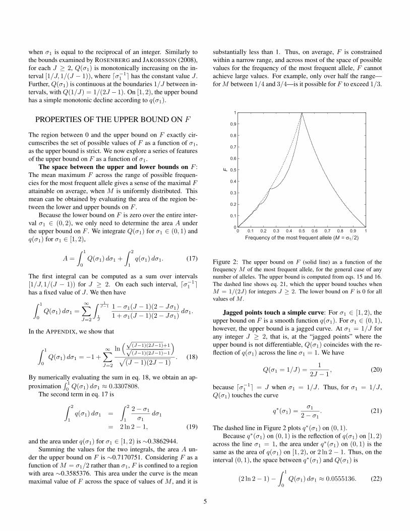
The upper bound on F is shown as the solid line in Fig-ure 2. The plot illustrates that the upper bound on F (σ1) has apiecewise structure on (0, 1), with changes in shape occurring

4

when σ1 is equal to the reciprocal of an integer. Similarly tothe bounds examined by ROSENBERG and JAKOBSSON (2008),for each J ≥ 2, Q(σ1) is monotonically increasing on the in-terval [1/J, 1/(J − 1)), where ⌈σ−1

1 ⌉ has the constant value J .Further, Q(σ1) is continuous at the boundaries 1/J between in-tervals, with Q(1/J) = 1/(2J − 1). On [1, 2), the upper boundhas a simple monotonic decline according to q(σ1).

PROPERTIES OF THE UPPER BOUND ON F

The region between 0 and the upper bound on F exactly cir-cumscribes the set of possible values of F as a function of σ1,as the upper bound is strict. We now explore a series of featuresof the upper bound on F as a function of σ1.

The space between the upper and lower bounds on F :The mean maximum F across the range of possible frequen-cies for the most frequent allele gives a sense of the maximal Fattainable on average, when M is uniformly distributed. Thismean can be obtained by evaluating the area of the region be-tween the lower and upper bounds on F .

Because the lower bound on F is zero over the entire inter-val σ1 ∈ (0, 2), we only need to determine the area A underthe upper bound on F . We integrate Q(σ1) for σ1 ∈ (0, 1) andq(σ1) for σ1 ∈ [1, 2),

A =

∫ 1

0

Q(σ1) dσ1 +

∫ 2

1

q(σ1) dσ1. (17)

The first integral can be computed as a sum over intervals[1/J, 1/(J − 1)) for J ≥ 2. On each such interval, ⌈σ−1

1 ⌉has a fixed value of J . We then have∫ 1

0

Q(σ1) dσ1 =∞∑

J=2

∫ 1J−1

1J

1− σ1(J − 1)(2− Jσ1)

1 + σ1(J − 1)(2− Jσ1)dσ1.

In the APPENDIX, we show that

∫ 1

0

Q(σ1) dσ1 = −1 +

∞∑J=2

ln(√

(J−1)(2J−1)+1√(J−1)(2J−1)−1

)√(J − 1)(2J − 1)

. (18)

By numerically evaluating the sum in eq. 18, we obtain an ap-proximation

∫ 1

0Q(σ1) dσ1 ≈ 0.3307808.

The second term in eq. 17 is∫ 2

1

q(σ1) dσ1 =

∫ 2

1

2− σ1

σ1dσ1

= 2 ln 2− 1, (19)

and the area under q(σ1) for σ1 ∈ [1, 2) is ∼0.3862944.Summing the values for the two integrals, the area A un-

der the upper bound on F is ∼0.7170751. Considering F as afunction of M = σ1/2 rather than σ1, F is confined to a regionwith area ∼0.3585376. This area under the curve is the meanmaximal value of F across the space of values of M , and it is

substantially less than 1. Thus, on average, F is constrainedwithin a narrow range, and across most of the space of possiblevalues for the frequency of the most frequent allele, F cannotachieve large values. For example, only over half the range—for M between 1/4 and 3/4—is it possible for F to exceed 1/3.

Frequency of the most frequent allele (M = σ1 2)

F

0 0.1 0.2 0.3 0.4 0.5 0.6 0.7 0.8 0.9 10

0.1

0.2

0.3

0.4

0.5

0.6

0.7

0.8

0.9

1

Figure 2: The upper bound on F (solid line) as a function of thefrequency M of the most frequent allele, for the general case of anynumber of alleles. The upper bound is computed from eqs. 15 and 16.The dashed line shows eq. 21, which the upper bound touches whenM = 1/(2J) for integers J ≥ 2. The lower bound on F is 0 for allvalues of M .

Jagged points touch a simple curve: For σ1 ∈ [1, 2), theupper bound on F is a smooth function q(σ1). For σ1 ∈ (0, 1),however, the upper bound is a jagged curve. At σ1 = 1/J forany integer J ≥ 2, that is, at the “jagged points” where theupper bound is not differentiable, Q(σ1) coincides with the re-flection of q(σ1) across the line σ1 = 1. We have

Q(σ1 = 1/J) =1

2J − 1, (20)

because ⌈σ−11 ⌉ = J when σ1 = 1/J . Thus, for σ1 = 1/J ,

Q(σ1) touches the curve

q∗(σ1) =σ1

2− σ1. (21)

The dashed line in Figure 2 plots q∗(σ1) on (0, 1).Because q∗(σ1) on (0, 1) is the reflection of q(σ1) on [1, 2)

across the line σ1 = 1, the area under q∗(σ1) on (0, 1) is thesame as the area of q(σ1) on [1, 2), or 2 ln 2 − 1. Thus, on theinterval (0, 1), the space between q∗(σ1) and Q(σ1) is

(2 ln 2− 1)−∫ 1

0

Q(σ1) dσ1 ≈ 0.0555136. (22)

5

The contribution made by M to the upper bound on F :We denote by F1(σ1) the contribution of the most frequent al-lele to F (σ1). By this quantity, we mean the term in F (σ1) con-tributed by the difference between populations in the frequencyof the most frequent allele. From eq. 4, F (σ1) can be written

F (σ1) =I∑

i=1

δ2i

4−∑I

j=1 σ2j

. (23)

If the ith term in the summation is denoted Fi(σ1), our interestis in the value of F1(σ1) obtained at the set of allele frequenciesthat maximizes F (σ1).

For σ1 in the interval (0, 1), defining ⌈σ−11 ⌉ = J , the maxi-

mum has 2J − 2 alleles with frequency σ1 and two alleles withfrequency 1−(J−1)σ1: J−1 alleles with frequency σ1 and oneallele with frequency 1− (J − 1)σ1 in each subpopulation. Thevalue of δ21 at the maximum is σ2

1 . Denoting the contributionF1(σ1) to F (σ1) at the maximum by Q1(σ1), we have

Q1(σ1) =σ21

2 + 2σ1(⌈σ−11 ⌉ − 1)(2− ⌈σ−1

1 ⌉σ1). (24)

In the APPENDIX, we evaluate∫ 1

0Q1(σ1) dσ1. The expres-

sion is unwieldy, but it provides a numerical approximation∫ 1

0Q1(σ1) dσ1 ≈ 0.1284522.For σ1 ∈ [1, 2), at the maximum of F (σ1), δ21 = (2− σ1)

2,and we have

q1(σ1) =(2− σ1)

2

4− σ21 − (2− σ1)2

=2− σ1

2σ1. (25)

The area under q1(σ1) is∫ 2

1

q1(σ1) dσ1 = ln 2− 1

2≈ 0.1931472.

Summing the areas under Q1(σ1) and q1(σ1), the total areaB under F1 as σ1 ranges from 0 to 2 is

B =

∫ 1

0

Q1(σ1) dσ1 +

∫ 2

1

q1(σ1) dσ1 ≈ 0.3215994.

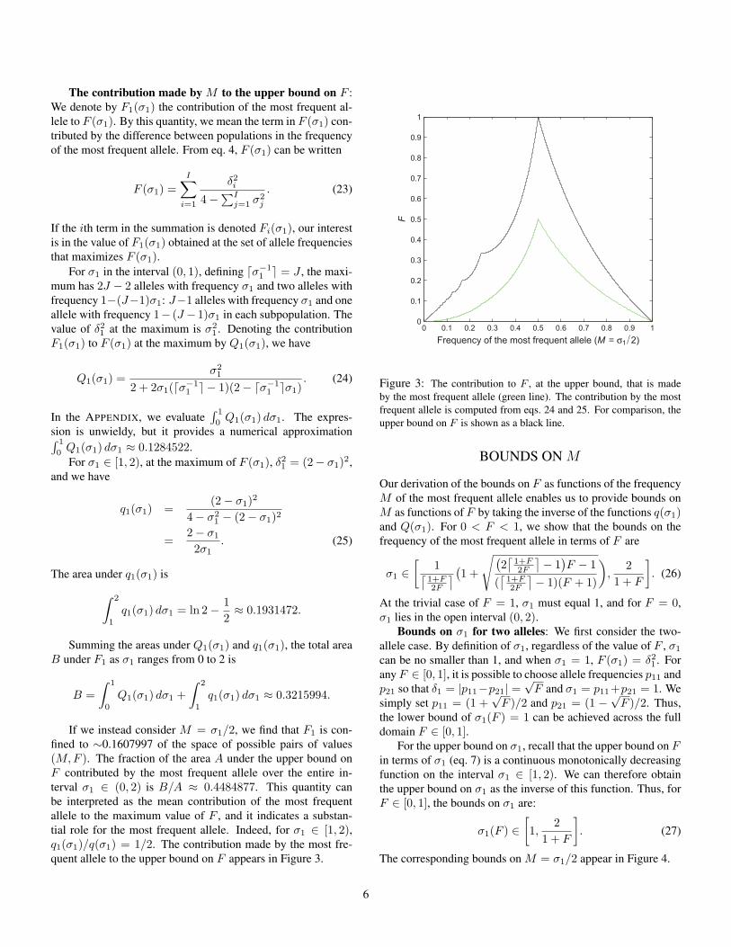
If we instead consider M = σ1/2, we find that F1 is con-fined to ∼0.1607997 of the space of possible pairs of values(M,F ). The fraction of the area A under the upper bound onF contributed by the most frequent allele over the entire in-terval σ1 ∈ (0, 2) is B/A ≈ 0.4484877. This quantity canbe interpreted as the mean contribution of the most frequentallele to the maximum value of F , and it indicates a substan-tial role for the most frequent allele. Indeed, for σ1 ∈ [1, 2),q1(σ1)/q(σ1) = 1/2. The contribution made by the most fre-quent allele to the upper bound on F appears in Figure 3.

Frequency of the most frequent allele (M = σ1 2)

F

0 0.1 0.2 0.3 0.4 0.5 0.6 0.7 0.8 0.9 10

0.1

0.2

0.3

0.4

0.5

0.6

0.7

0.8

0.9

1

Figure 3: The contribution to F , at the upper bound, that is madeby the most frequent allele (green line). The contribution by the mostfrequent allele is computed from eqs. 24 and 25. For comparison, theupper bound on F is shown as a black line.

BOUNDS ON M

Our derivation of the bounds on F as functions of the frequencyM of the most frequent allele enables us to provide bounds onM as functions of F by taking the inverse of the functions q(σ1)and Q(σ1). For 0 < F < 1, we show that the bounds on thefrequency of the most frequent allele in terms of F are

σ1 ∈[

1⌈1+F2F

⌉(1 +√(2⌈1+F2F

⌉− 1)F − 1

(⌈1+F2F

⌉− 1)(F + 1)

),

2

1 + F

]. (26)

At the trivial case of F = 1, σ1 must equal 1, and for F = 0,σ1 lies in the open interval (0, 2).

Bounds on σ1 for two alleles: We first consider the two-allele case. By definition of σ1, regardless of the value of F , σ1

can be no smaller than 1, and when σ1 = 1, F (σ1) = δ21 . Forany F ∈ [0, 1], it is possible to choose allele frequencies p11 andp21 so that δ1 = |p11−p21| =

√F and σ1 = p11+p21 = 1. We

simply set p11 = (1 +√F )/2 and p21 = (1 −

√F )/2. Thus,

the lower bound of σ1(F ) = 1 can be achieved across the fulldomain F ∈ [0, 1].

For the upper bound on σ1, recall that the upper bound on Fin terms of σ1 (eq. 7) is a continuous monotonically decreasingfunction on the interval σ1 ∈ [1, 2). We can therefore obtainthe upper bound on σ1 as the inverse of this function. Thus, forF ∈ [0, 1], the bounds on σ1 are:

σ1(F ) ∈[1,

2

1 + F

]. (27)

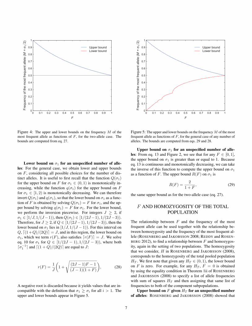
The corresponding bounds on M = σ1/2 appear in Figure 4.

6

F

Fre

quency o

f th

e m

ost

frequent

alle

le (M

= σ

12)

0 0.1 0.2 0.3 0.4 0.5 0.6 0.7 0.8 0.9 10

0.1

0.2

0.3

0.4

0.5

0.6

0.7

0.8

0.9

1

Upper boundLower bound

Figure 4: The upper and lower bounds on the frequency M of themost frequent allele as functions of F , for the two-allele case. Thebounds are computed from eq. 27.

Lower bound on σ1 for an unspecified number of alle-les: For the general case, we obtain lower and upper boundson F , considering all possible choices for the number of dis-tinct alleles. It is useful to first recall that the function Q(σ1)for the upper bound on F for σ1 ∈ (0, 1) is monotonically in-creasing, while the function q(σ1) for the upper bound on Ffor σ1 ∈ [1, 2) is monotonically decreasing. We can thereforeinvert Q(σ1) and q(σ1), so that the lower bound on σ1 as a func-tion of F is obtained by solving Q(σ1) = F for σ1, and the up-per bound by solving q(σ1) = F for σ1. For the lower bound,we perform the inversion piecewise. For integers J ≥ 2, ifσ1 ∈ [1/J, 1/(J−1)), then Q(σ1) ∈ [1/(2J−1), 1/(2J−3)).Therefore, for J ≥ 2, if Q ∈ [1/(2J−1), 1/(2J−3)), then thelower bound on σ1 lies in [1/J, 1/(J − 1)). For this interval onQ, ⌈(1+Q)/(2Q)⌉ = J , and in this region, the lower bound onσ1, which we term r(F ), also satisfies ⌈r(F )⌉ = J . We solveeq. 10 for σ1 for Q ∈ [1/(2J − 1), 1/(2J − 3)), where both⌈σ−1

1 ⌉ and ⌈(1 +Q)/(2Q)⌉ are equal to J :

r(F ) =1

J

(1 +

√(2J − 1)F − 1

(J − 1)(1 + F )

), (28)

A negative root is discarded because it yields values that are in-compatible with the definition that σ1 ≥ σi for all i > 1. Theupper and lower bounds appear in Figure 5.

F

Fre

quency o

f th

e m

ost

frequent

alle

le (M

= σ

12)

0 0.1 0.2 0.3 0.4 0.5 0.6 0.7 0.8 0.9 10

0.1

0.2

0.3

0.4

0.5

0.6

0.7

0.8

0.9

1

Upper boundLower bound

Figure 5: The upper and lower bounds on the frequency M of the mostfrequent allele as functions of F , for the general case of any number ofalleles. The bounds are computed from eqs. 29 and 28.

Upper bound on σ1 for an unspecified number of alle-les: From eq. 13 and Figure 2, we see that for any F ∈ [0, 1],the upper bound on σ1 is greater than or equal to 1. Becauseeq. 13 is continuous and monotonically decreasing, we can takethe inverse of this function to compute the upper bound on σ1

as a function of F . The upper bound R(F ) on σ1 is

R(F ) =2

1 + F, (29)

the same upper bound as for the two-allele case (eq. 27).

F AND HOMOZYGOSITY OF THE TOTALPOPULATION

The relationship between F and the frequency of the mostfrequent allele can be used together with the relationship be-tween homozygosity and the frequency of the most frequent al-lele (ROSENBERG and JAKOBSSON 2008; REDDY and ROSEN-BERG 2012), to find a relationship between F and homozygos-ity, again in the setting of two populations. The homozygositythat we consider, H in ROSENBERG and JAKOBSSON (2008),corresponds to the homozygosity of the total pooled populationHT . We first note that given any HT ∈ (0, 1), the lower boundon F is zero. For example, for any HT , F = 0 is obtainedby using the equality condition in Theorem 1ii of ROSENBERGand JAKOBSSON (2008) to specify a list of allele frequencieswith sum of squares HT and then assigning that same list offrequencies to both of the component subpopulations.

Upper bound on F given HT for an unspecified numberof alleles: ROSENBERG and JAKOBSSON (2008) showed that

7

the value of HT constrains the frequency M of the most fre-quent allele to a narrow range. We have already determined theupper bound on F as a function of M . Thus, we can obtain anupper bound on F as a function of HT by taking the maximumvalue of the upper bound over the range of possible values ofM allowed under the results of ROSENBERG and JAKOBSSON(2008) for a given value of HT . This approach does not guar-antee that the upper bound on F that we obtain in terms of HT

is strict; nevertheless, the approach happens to produce a strictbound for HT ∈ [1/2, 1). For HT ∈ (0, 1/2), it is possible toproduce a strict bound by writing F in terms of HT .

To obtain the bound for HT ∈ (0, 1/2), we substituteσ2i − 4p1ip2i for δ2i in eq. 4 to write

F =HT −

∑Ii=1 p1ip2i

1−HT. (30)

Because∑1

i=1 p1ip2i ≥ 0, we obtain the bound

F ≤ HT

1−HT. (31)

Given HT , equality is obtained in eq. 31 when∑I

i=1 p1ip2i =0. In other words, for HT ∈ (0, 1/2), F is maximized wheneach allele occurs in only one of the two populations. To seethat the upper bound is strict, note that when

∑Ii=1 p1ip2i = 0,

labeling the homozygosities of the two populations by H1 andH2, HT = (H1 + H2)/4. As HT < 1/2, 2HT < 1, and wecan choose H1 = H2 = 2HT . Using the equality condition inTheorem 1ii of ROSENBERG and JAKOBSSON (2008), we canspecify a set L of exactly ⌈(2HT )

−1⌉ allele frequencies whosesum of squares is HT . We then construct a set of 2⌈(2HT )

−1⌉alleles. In population 1, the first ⌈(2HT )

−1⌉ alleles in the sethave exactly the allele frequencies in L and the next ⌈(2HT )

−1⌉alleles have frequency 0. In population 2, the first ⌈(2HT )

−1⌉alleles have frequency 0, and the next ⌈(2HT )

−1⌉ alleles havethe frequencies in L.

For HT ∈ [1/2, 1), HT /(1 − HT ) ≥ 1, so eq. 31 pro-vides only the trivial bound of F ≤ 1, and another approach isneeded. For any HT ∈ [1/2, 1), using Theorem 1ii of ROSEN-BERG and JAKOBSSON (2008), M ≥ 1/2. For M ≥ 1/2, theupper bound on F as a function of σ1 is monotonically decreas-ing in σ1, and consequently, the upper bound on F as a functionof HT is obtained by evaluating q(σ1) at the smallest value ofσ1 permitted by HT . Theorem 1ii of ROSENBERG and JAKOB-SSON (2008) indicates that this smallest allowed σ1 satisfies

σ1/2 = M =1

⌈H−1T ⌉

(1 +

√⌈H−1

T ⌉HT − 1√⌈H−1

T ⌉ − 1

).

By replacing σ1/2 in eq. 16 with this expression, we have

F ≤⌈H−1

T ⌉

1 +

√⌈H−1

T ⌉HT−1√⌈H−1

T ⌉−1

− 1

=1−

√2HT − 1

1 +√2HT − 1

, (32)

where the last step follows from the fact that ⌈H−1T ⌉ = 2 when

HT ∈ [1/2, 1).For HT ∈ [1/2, 1), the set of allele frequencies that achieves

the minimum M as a function of HT and the set that achievesthe maximum F as a function of M coincide. Given HT ,M is minimized by setting p̄1 = (1 +

√2HT − 1)/2, p̄2 =

(1 −√2HT − 1)/2, and p̄i = 0 for all i ≥ 2. If these mean

frequencies are distributed between the two populations suchthat (p11, p12, p21, p22) = (1, 0,

√2HT − 1, 1−

√2HT − 1) or

(√2HT − 1, 1 −

√2HT − 1, 1, 0), then the upper bound on F

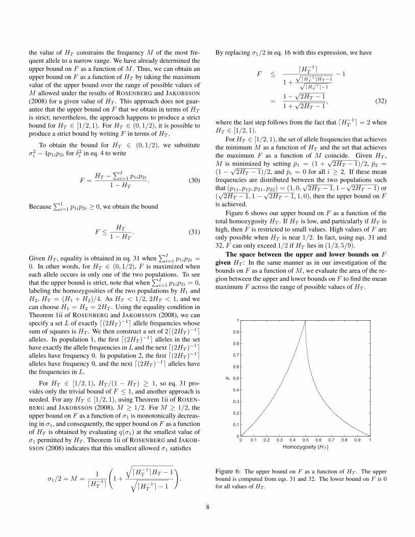
is achieved.Figure 6 shows our upper bound on F as a function of the

total homozygosity HT . If HT is low, and particularly if HT ishigh, then F is restricted to small values. High values of F areonly possible when HT is near 1/2. In fact, using eqs. 31 and32, F can only exceed 1/2 if HT lies in (1/3, 5/9).

The space between the upper and lower bounds on Fgiven HT : In the same manner as in our investigation of thebounds on F as a function of M , we evaluate the area of the re-gion between the upper and lower bounds on F to find the meanmaximum F across the range of possible values of HT .

Homozygosity (HT)

F

0 0.1 0.2 0.3 0.4 0.5 0.6 0.7 0.8 0.9 10

0.1

0.2

0.3

0.4

0.5

0.6

0.7

0.8

0.9

1

Figure 6: The upper bound on F as a function of HT . The upperbound is computed from eqs. 31 and 32. The lower bound on F is 0for all values of HT .

8

Because the lower bound on F is zero over the entire in-terval HT ∈ (0, 1), it suffices to evaluate the area A under theupper bound on F . This area is

A =

∫ 1/2

0

HT

1−HTdHT +

∫ 1

1/2

1−√2HT − 1

1 +√2HT − 1

dHT . (33)

The first term has indefinite integral −HT − ln(1 − HT ) andevaluates to ln 2 − 1/2. The second term has indefinite inte-gral −HT +2

√2H − 1− 2 ln(1+

√2H − 1) and evaluates to

3/2− 2 ln 2, so that A = 1− ln 2 ≈ 0.3068528.

Note that F is substantially more constrained when HT ∈[1/2, 1) than when HT ∈ (0, 1/2). The difference betweenthe areas under the upper bound for HT ∈ (0, 1/2) and forHT ∈ [1/2, 1) is 3 ln 2 − 2 ≈ 0.0794415, a sizeable fractionof the sum of the two areas. Twice the difference in areas, or6 ln 2 − 4 ≈ 0.1588831, is the expectation of the differencebetween the maximum value of F for a value of HT chosenuniformly at random from (0, 1/2) and the maximum value ofF for a value of HT chosen uniformly at random from [1/2, 1).

APPLICATION TO DATA

We illustrate the bounds on F , M , and HT for a series of exam-ples using human polymorphism data from ROSENBERG et al.(2005) and LI et al. (2008). For each example, for each locus,we assume that the allele frequencies in the data sets are para-metric allele frequencies. The parametric allele frequencies areobtained in each of a pair of populations, and they are then aver-aged to obtain parametric allele frequencies for the total popula-tion. F , M , and HT are then computed. The data set of ROSEN-BERG et al. (2005) considers 1048 individuals genotyped for783 microsatellites, and the data set of LI et al. (2008) consid-ers 938 unrelated individuals genotyped for single-nucleotidepolymorphisms (SNPs); for all analyses, we restrict our atten-tion to the 935 individuals found in both data sets. For the LIet al. (2008) data, we only examine 640,034 SNPs studied byPEMBERTON et al. (2012).

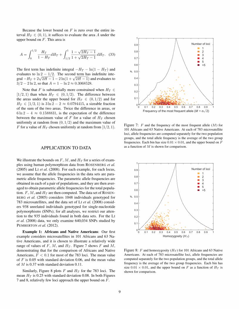
Example 1: Africans and Native Americans: Our firstexample considers microsatellites in 101 Africans and 63 Na-tive Americans, and it is chosen to illustrate a relatively widerange of values of F , M , and HT . Figure 7 shows F and M ,demonstrating that for the comparison of Africans and NativeAmericans, F < 0.1 for most of the 783 loci. The mean valueof F is 0.05 with standard deviation 0.06, and the mean valueof M is 0.37 with standard deviation 0.11.

Similarly, Figure 8 plots F and HT for the 783 loci. Themean HT is 0.25 with standard deviation 0.08. In both Figures7 and 8, relatively few loci approach the upper bound on F .

Frequency of the most frequent allele (M = σ1 2)

F

0 0.1 0.2 0.3 0.4 0.5 0.6 0.7 0.8 0.9 10

0.1

0.2

0.3

0.4

0.5

0.6

0.7

0.8

0.9

1

Number of loci

12345>5

Figure 7: F and the frequency of the most frequent allele (M ) for101 Africans and 63 Native Americans. At each of 783 microsatelliteloci, allele frequencies are computed separately for the two populationgroups, and the total allele frequency is the average of the two groupfrequencies. Each bin has size 0.01× 0.01, and the upper bound on Fas a function of M is shown for comparison.

Homozygosity (HT)

F

0 0.1 0.2 0.3 0.4 0.5 0.6 0.7 0.8 0.9 10

0.1

0.2

0.3

0.4

0.5

0.6

0.7

0.8

0.9

1

Number of loci

12345>5

Figure 8: F and homozygosity (HT ) for 101 Africans and 63 NativeAmericans. At each of 783 microsatellite loci, allele frequencies arecomputed separately for the two population groups, and the total allelefrequency is the average of the two group frequencies. Each bin hassize 0.01 × 0.01, and the upper bound on F as a function of HT isshown for comparison.

9

Frequency of the most frequent allele (M = σ1 2)

F

0 0.2 0.4 0.6 0.8 10

0.1

0.2

0.3

0.4

0.5

0.6

0.7

0.8

0.9

1

Number of loci

1

2

3

4

5

>5

A)

Homozygosity (HT)F

0 0.2 0.4 0.6 0.8 10

0.1

0.2

0.3

0.4

0.5

0.6

0.7

0.8

0.9

1

Number of loci

1

2

3

4

5

>5

B)

Frequency of the most frequent allele (M = σ1 2)

F

0 0.2 0.4 0.6 0.8 10

0.1

0.2

0.3

0.4

0.5

0.6

0.7

0.8

0.9

1

Number of loci

1

2

3

4

5

>5

C)

Homozygosity (HT)

F

0 0.2 0.4 0.6 0.8 10

0.1

0.2

0.3

0.4

0.5

0.6

0.7

0.8

0.9

1

Number of loci

1

2

3

4

5

>5

D)

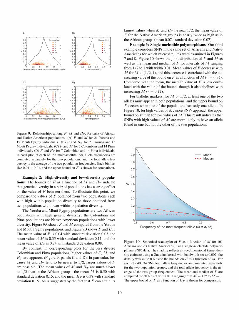
Figure 9: Relationships among F , M and HT , for pairs of Africanand Native American populations. (A) F and M for 21 Yoruba and15 Mbuti Pygmy individuals. (B) F and HT for 21 Yoruba and 15Mbuti Pygmy individuals. (C) F and M for 7 Colombian and 14 Pimaindividuals. (D) F and HT for 7 Colombian and 14 Pima individuals.In each plot, at each of 783 microsatellite loci, allele frequencies arecomputed separately for the two populations, and the total allele fre-quency is the average of the two population frequencies. Each bin hassize 0.01× 0.01, and the upper bound on F is shown for comparison.

Example 2: High-diversity and low-diversity popula-tions: The bounds on F as a function of M and HT indicatethat genetic diversity in a pair of populations has a strong effecton the value of F between them. To illustrate this point, wecompare the values of F obtained from two populations eachwith high within-population diversity to those obtained fromtwo populations with lower within-population diversity.

The Yoruba and Mbuti Pygmy populations are two Africanpopulations with high genetic diversity; the Colombian andPima populations are Native American populations with lowerdiversity. Figure 9A shows F and M computed from the Yorubaand Mbuti Pygmy populations, and Figure 9B shows F and HT .The mean value of F is 0.04 with standard deviation 0.03, themean value of M is 0.35 with standard deviation 0.11, and themean value of HT is 0.24 with standard deviation 0.08.

By contrast, in corresponding plots for the less diverseColombian and Pima populations, higher values of F , M , andHT are apparent (Figure 9, panels C and D). In particular, be-cause M and HT tend to be nearer to 1/2, larger values of Fare possible. The mean values of M and HT are much closerto 1/2 than in the African groups; the mean M is 0.50 withstandard deviation 0.15, and the mean HT is 0.38 with standarddeviation 0.15. As is suggested by the fact that F can attain its

largest values when M and HT lie near 1/2, the mean value ofF for the Native American groups is nearly twice as high as inthe African groups (mean 0.07, standard deviation 0.07).

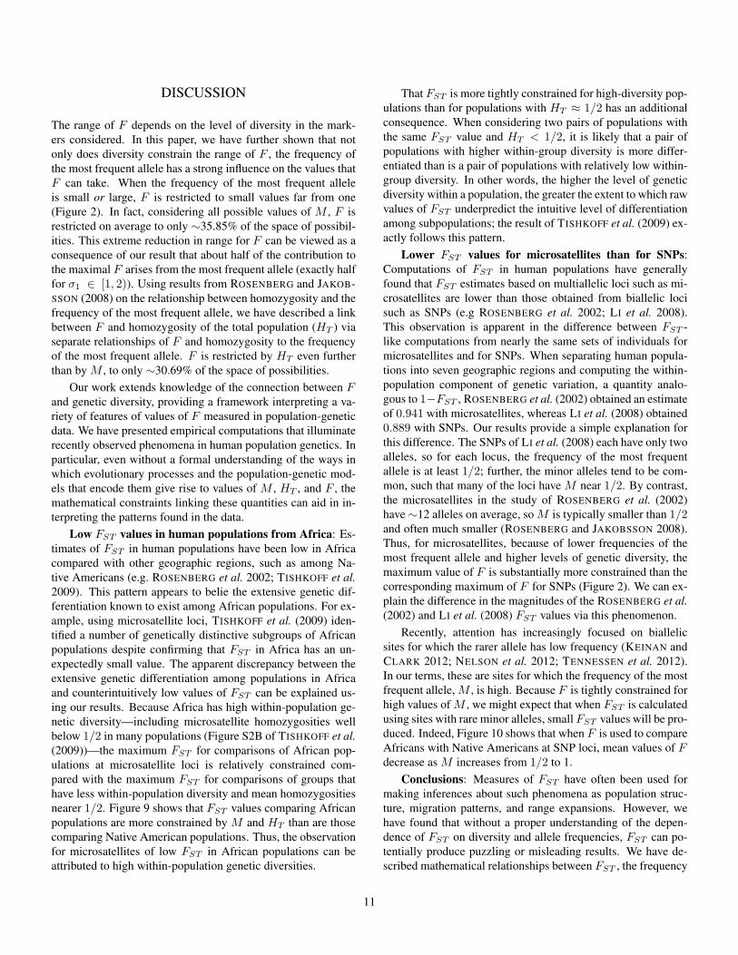
Example 3: Single-nucleotide polymorphisms: Our thirdexample considers SNPs in the same set of Africans and NativeAmericans for which microsatellites were examined in Figures7 and 8. Figure 10 shows the joint distribution of F and M aswell as the mean and median of F for intervals of M rangingfrom 1/2 to 1 with width 0.01. Mean values of F decrease withM for M ∈ (1/2, 1), and this decrease is correlated with the de-creasing value of the bound on F as a function of M (r = 0.94).Compared with the mean, the median value of F is less corre-lated with the value of the bound, though it also declines withincreasing M (r = 0.77).

For biallelic markers, for M > 1/2, at least one of the twoalleles must appear in both populations, and the upper bound onF occurs when one of the populations has only one allele. InFigure 10, for high values of M , more SNPs approach the upperbound on F than for low values of M . This result indicates thatSNPs with high values of M are more likely to have an allelefound in one but not the other of the two populations.

Frequency of the most frequent allele (M = σ1 2)

F

0.5 0.6 0.7 0.8 0.9 10

0.1

0.2

0.3

0.4

0.5

0.6

0.7

0.8

0.9

1

MeanMedian

Figure 10: Smoothed scatterplot of F as a function of M for 101Africans and 63 Native Americans, using single-nucleotide polymor-phism (SNP) data. The shading reflects a two-dimensional kernel den-sity estimate using a Gaussian kernel with bandwidth set to 0.007; thedensity was set to 0 outside the bounds on F as a function of M . Foreach of 640,034 SNP loci, allele frequencies are computed separatelyfor the two population groups, and the total allele frequency is the av-erage of the two group frequencies. The mean and median of F arecomputed for 50 bins of width 0.01 ranging from M = 1/2 to M = 1.The upper bound on F as a function of HT is shown for comparison.

10

DISCUSSION

The range of F depends on the level of diversity in the mark-ers considered. In this paper, we have further shown that notonly does diversity constrain the range of F , the frequency ofthe most frequent allele has a strong influence on the values thatF can take. When the frequency of the most frequent alleleis small or large, F is restricted to small values far from one(Figure 2). In fact, considering all possible values of M , F isrestricted on average to only ∼35.85% of the space of possibil-ities. This extreme reduction in range for F can be viewed as aconsequence of our result that about half of the contribution tothe maximal F arises from the most frequent allele (exactly halffor σ1 ∈ [1, 2)). Using results from ROSENBERG and JAKOB-SSON (2008) on the relationship between homozygosity and thefrequency of the most frequent allele, we have described a linkbetween F and homozygosity of the total population (HT ) viaseparate relationships of F and homozygosity to the frequencyof the most frequent allele. F is restricted by HT even furtherthan by M , to only ∼30.69% of the space of possibilities.

Our work extends knowledge of the connection between Fand genetic diversity, providing a framework interpreting a va-riety of features of values of F measured in population-geneticdata. We have presented empirical computations that illuminaterecently observed phenomena in human population genetics. Inparticular, even without a formal understanding of the ways inwhich evolutionary processes and the population-genetic mod-els that encode them give rise to values of M , HT , and F , themathematical constraints linking these quantities can aid in in-terpreting the patterns found in the data.

Low FST values in human populations from Africa: Es-timates of FST in human populations have been low in Africacompared with other geographic regions, such as among Na-tive Americans (e.g. ROSENBERG et al. 2002; TISHKOFF et al.2009). This pattern appears to belie the extensive genetic dif-ferentiation known to exist among African populations. For ex-ample, using microsatellite loci, TISHKOFF et al. (2009) iden-tified a number of genetically distinctive subgroups of Africanpopulations despite confirming that FST in Africa has an un-expectedly small value. The apparent discrepancy between theextensive genetic differentiation among populations in Africaand counterintuitively low values of FST can be explained us-ing our results. Because Africa has high within-population ge-netic diversity—including microsatellite homozygosities wellbelow 1/2 in many populations (Figure S2B of TISHKOFF et al.(2009))—the maximum FST for comparisons of African pop-ulations at microsatellite loci is relatively constrained com-pared with the maximum FST for comparisons of groups thathave less within-population diversity and mean homozygositiesnearer 1/2. Figure 9 shows that FST values comparing Africanpopulations are more constrained by M and HT than are thosecomparing Native American populations. Thus, the observationfor microsatellites of low FST in African populations can beattributed to high within-population genetic diversities.

That FST is more tightly constrained for high-diversity pop-ulations than for populations with HT ≈ 1/2 has an additionalconsequence. When considering two pairs of populations withthe same FST value and HT < 1/2, it is likely that a pair ofpopulations with higher within-group diversity is more differ-entiated than is a pair of populations with relatively low within-group diversity. In other words, the higher the level of geneticdiversity within a population, the greater the extent to which rawvalues of FST underpredict the intuitive level of differentiationamong subpopulations; the result of TISHKOFF et al. (2009) ex-actly follows this pattern.

Lower FST values for microsatellites than for SNPs:Computations of FST in human populations have generallyfound that FST estimates based on multiallelic loci such as mi-crosatellites are lower than those obtained from biallelic locisuch as SNPs (e.g ROSENBERG et al. 2002; LI et al. 2008).This observation is apparent in the difference between FST -like computations from nearly the same sets of individuals formicrosatellites and for SNPs. When separating human popula-tions into seven geographic regions and computing the within-population component of genetic variation, a quantity analo-gous to 1−FST , ROSENBERG et al. (2002) obtained an estimateof 0.941 with microsatellites, whereas LI et al. (2008) obtained0.889 with SNPs. Our results provide a simple explanation forthis difference. The SNPs of LI et al. (2008) each have only twoalleles, so for each locus, the frequency of the most frequentallele is at least 1/2; further, the minor alleles tend to be com-mon, such that many of the loci have M near 1/2. By contrast,the microsatellites in the study of ROSENBERG et al. (2002)have ∼12 alleles on average, so M is typically smaller than 1/2and often much smaller (ROSENBERG and JAKOBSSON 2008).Thus, for microsatellites, because of lower frequencies of themost frequent allele and higher levels of genetic diversity, themaximum value of F is substantially more constrained than thecorresponding maximum of F for SNPs (Figure 2). We can ex-plain the difference in the magnitudes of the ROSENBERG et al.(2002) and LI et al. (2008) FST values via this phenomenon.

Recently, attention has increasingly focused on biallelicsites for which the rarer allele has low frequency (KEINAN andCLARK 2012; NELSON et al. 2012; TENNESSEN et al. 2012).In our terms, these are sites for which the frequency of the mostfrequent allele, M , is high. Because F is tightly constrained forhigh values of M , we might expect that when FST is calculatedusing sites with rare minor alleles, small FST values will be pro-duced. Indeed, Figure 10 shows that when F is used to compareAfricans with Native Americans at SNP loci, mean values of Fdecrease as M increases from 1/2 to 1.

Conclusions: Measures of FST have often been used formaking inferences about such phenomena as population struc-ture, migration patterns, and range expansions. However, wehave found that without a proper understanding of the depen-dence of FST on diversity and allele frequencies, FST can po-tentially produce puzzling or misleading results. We have de-scribed mathematical relationships between FST , the frequency

11

of the most frequent allele, and homozygosity that are usefulfor interpreting the properties of differentiation measures whenfeatures of allele frequencies and diversity statistics vary acrossloci or populations—as they inevitably do in typical scenarios.

Beginning with CHARLESWORTH (1998), NAGYLAKI(1998), and HEDRICK (1999), recent studies have noted thatFST is constrained by diversity, and the issue was described asearly as in the work of Sewall Wright (WRIGHT 1978, p. 82).JOST (2008) generated new interest in the dependence of FST

on diversity, illustrating that the dependence can produce sub-stantial discord between intuitions about and measurements ofdifferentiation levels. JOST (2008) also used a multiplicativedefinition of diversity to propose a pair of new differentiationindices that have the feature of reaching their maximum valueif and only if each allele is private to a single subpopulation. Inour view, the key to choosing and applying measures of differ-entiation lies not in “fixation on an index” (LONG 2009), be itFST , the measures of JOST (2008), or other indices that haverecently been proposed (MEIRMANS and HEDRICK 2011), butin developing an understanding of the ways in which possiblestatistics relate both to intuitive aspects of differentiation andto mathematical features of allele frequencies and genetic di-versity. In this context, FST remains of particular interest onthe basis of its long history of use in population genetics and itsconnection to features of biological models (WHITLOCK 2011).Our examples provide only a few among many ways in whichthe mathematical properties we have obtained for FST can beused to interpret its behavior in the analysis of empirical data.

We thank S. Boca and J. VanLiere for numerous discussions of thiswork. Financial support was provided by the Swedish Research Coun-cil Formas, the Erik Philip Sörensen Foundation, the Burroughs Well-come Fund, a Stanford Graduate Fellowship, and US National Insti-tutes of Health grant GM081441.

REFERENCES

BOCA, S. M., and N. A. ROSENBERG, 2011 Mathematical proper-ties of Fst between admixed populations and their parental sourcepopulations. Theor. Pop. Biol. 80: 208–216.

CHARLESWORTH, B., 1998 Measures of divergence between popula-tions and the effect of forces that reduce variability. Mol. Biol. Evol.15: 538–543.

HEDRICK, P. W., 1999 Perspective: highly variable loci and their in-terpretation in evolution and conservation. Evolution 53: 313–318.

HEDRICK, P. W., 2005 A standardized genetic differentiation measure.Evolution 59: 1633–1638.

HOLSINGER, K. E., and B. S. WEIR, 2009 Genetics in geographi-cally structured populations: defining, estimating and interpretingFST . Nature Rev. Genet. 10: 639–650.

JIN, L., and R. CHAKRABORTY, 1995 Population structure, stepwisemutations, heterozygote deficiency and their implications in DNAforensics. Heredity 74: 274–285.

JOST, L., 2008 GST and its relatives do not measure differentiation.Mol. Ecol. 17: 4015–4026.

KEINAN, A., and A. G. CLARK, 2012 Recent explosive human pop-ulation growth has resulted in an excess of rare genetic variants.Science 336: 740–743.

LI, J. Z., D. M. ABSHER, H. TANG, A. M. SOUTHWICK, A. M.CASTO, et al., 2008 Worldwide human relationships inferred fromgenome-wide patterns of variation. Science 319: 1100–1104.

LONG, J. C., 2009 Update to Long and Kittles’s “Human genetic di-versity and the nonexistence of biological races (2003): fixation onan index. Hum. Biol. 81: 799–803.

LONG, J. C., and R. A. KITTLES, 2003 Human genetic diversity andthe nonexistence of biological races. Hum. Biol. 75: 449–471.

MEIRMANS, P. G., and P. W. HEDRICK, 2011 Assessing populationstructure: FST and related measures. Mol. Ecol. Resources 11: 5–18.

NAGYLAKI, T., 1998 Fixation indices in subdivided populations. Ge-netics 148: 1325–1332.

NEI, M., 1973 Analysis of gene diversity in subdivided populations.Proc. Natl. Acad. Sci. USA 70: 3321–3323.

NELSON, M. R., D. WEGMANN, M. G. EHM, D. KESSNER, P. S.JEAN, et al., 2012 An abundance of rare functional variants in 202drug target genes sequenced in 14,002 people. Science 337: 100–104.

PEMBERTON, T. J., D. ABSHER, M. W. FELDMAN, R. M. MYERS,N. A. ROSENBERG, et al., 2012 Genomic patterns of homozygosityin worldwide human populations. Am. J. Hum. Genet. : in press.

REDDY, S. B., and N. A. ROSENBERG, 2012 Refining the relation-ship between homozygosity and the frequency of the most frequentallele. J. Math. Biol. 64: 87–108.

ROSENBERG, N. A., and M. JAKOBSSON, 2008 The relationship be-tween homozygosity and the frequency of the most frequent allele.Genetics 179: 2027–2036.

ROSENBERG, N. A., L. M. LI, R. WARD, and J. K. PRITCHARD,2003 Informativeness of genetic markers for inference of ancestry.Am. J. Hum. Genet. 73: 1402–1422.

ROSENBERG, N. A., S. MAHAJAN, S. RAMACHANDRAN, C. ZHAO,J. K. PRITCHARD, et al., 2005 Clines, clusters, and the effect ofstudy design on the inference of human population structure. PLoSGenet. 1: 660–671.

ROSENBERG, N. A., J. K. PRITCHARD, J. L. WEBER, H. M. CANN,K. K. KIDD, et al., 2002 Genetic structure of human populations.Science 298: 2381–2385.

RYMAN, N., and O. LEIMAR, 2008 Effect of mutation on geneticdifferentiation among nonequilibrium populations. Evolution 62:2250–2259.

TENNESSEN, J. A., A. W. BIGHAM, T. D. O’CONNOR, W. FU, E. E.KENNY, et al., 2012 Evolution and functional impact of rare cod-ing variation from deep sequencing of human exomes. Science 337:64–69.

TISHKOFF, S. A., F. A. REED, F. R. FRIEDLAENDER, C. EHRET,A. RANCIARO, et al., 2009 The genetic structure and history ofAfricans and African Americans. Science 324: 1035–1044.

WAHLUND, S., 1928 Zusammensetzung von Populationen und Korre-lationerscheinungen vom Standpunkt der Vererbungslehre aus Be-trachtet. Hereditas 11: 65–106.

WEIR, B. S., 1996 Genetic Data Analysis II. Sinauer, Sunderland,MA.

WHITLOCK, M. C., 2011 G′ST and D do not replace FST . Mol. Ecol.

20: 1083–1091.WRIGHT, S., 1951 The genetical structure of populations. Ann. Eugen.

15: 323–354.WRIGHT, S., 1978 Evolution and the Genetics of Populations Volume

4: Variability within and among Natural Populations. University ofChicago Press, Chicago.

12

APPENDIX

The appendix provides the derivations of two integrals described in the main text.

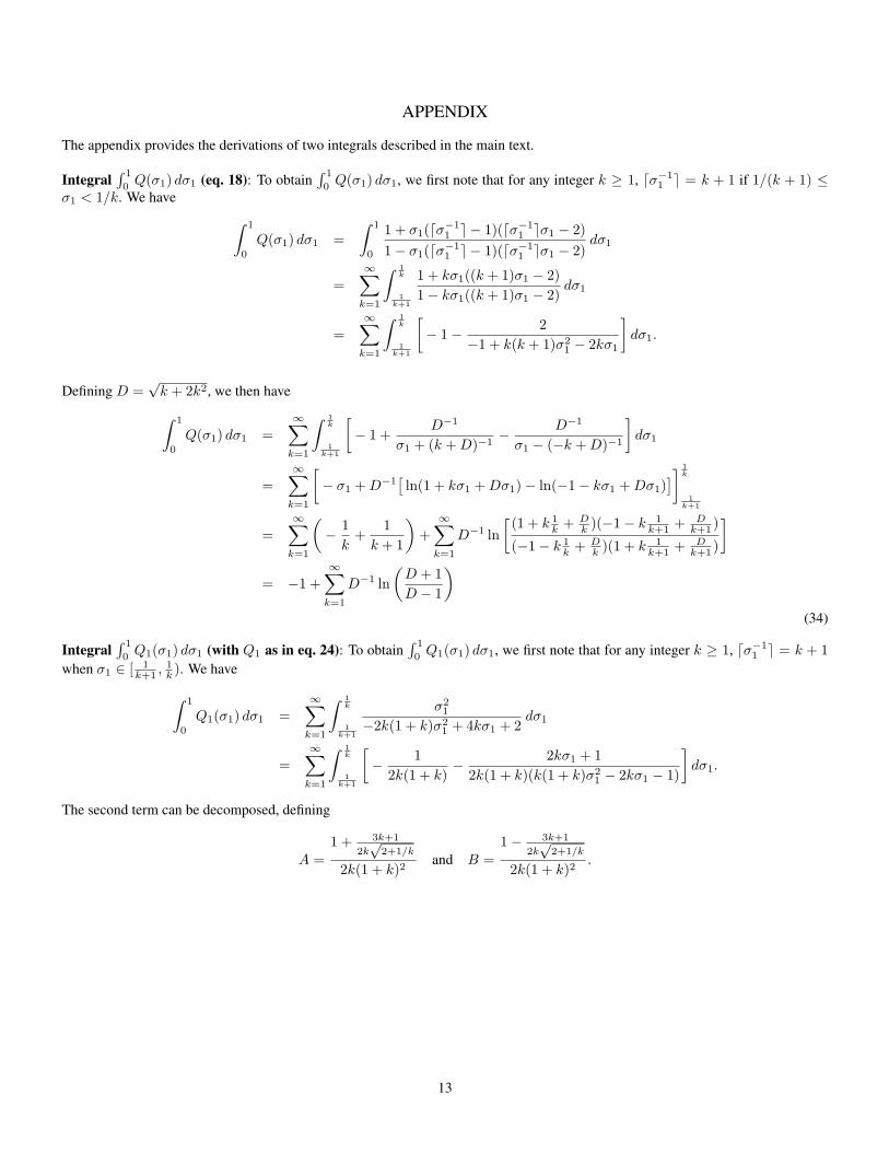
Integral∫ 1

0Q(σ1) dσ1 (eq. 18): To obtain

∫ 1

0Q(σ1) dσ1, we first note that for any integer k ≥ 1, ⌈σ−1

1 ⌉ = k + 1 if 1/(k + 1) ≤σ1 < 1/k. We have ∫ 1

0

Q(σ1) dσ1 =

∫ 1

0

1 + σ1(⌈σ−11 ⌉ − 1)(⌈σ−1

1 ⌉σ1 − 2)

1− σ1(⌈σ−11 ⌉ − 1)(⌈σ−1

1 ⌉σ1 − 2)dσ1

=∞∑k=1

∫ 1k

1k+1

1 + kσ1((k + 1)σ1 − 2)

1− kσ1((k + 1)σ1 − 2)dσ1

=

∞∑k=1

∫ 1k

1k+1

[− 1− 2

−1 + k(k + 1)σ21 − 2kσ1

]dσ1.

Defining D =√k + 2k2, we then have∫ 1

0

Q(σ1) dσ1 =∞∑k=1

∫ 1k

1k+1

[− 1 +

D−1

σ1 + (k +D)−1− D−1

σ1 − (−k +D)−1

]dσ1

=∞∑k=1

[− σ1 +D−1

[ln(1 + kσ1 +Dσ1)− ln(−1− kσ1 +Dσ1)

]] 1k

1k+1

=∞∑k=1

(− 1

k+

1

k + 1

)+

∞∑k=1

D−1 ln

[(1 + k 1

k + Dk )(−1− k 1

k+1 + Dk+1 )

(−1− k 1k + D

k )(1 + k 1k+1 + D

k+1 )

]

= −1 +∞∑k=1

D−1 ln

(D + 1

D − 1

)(34)

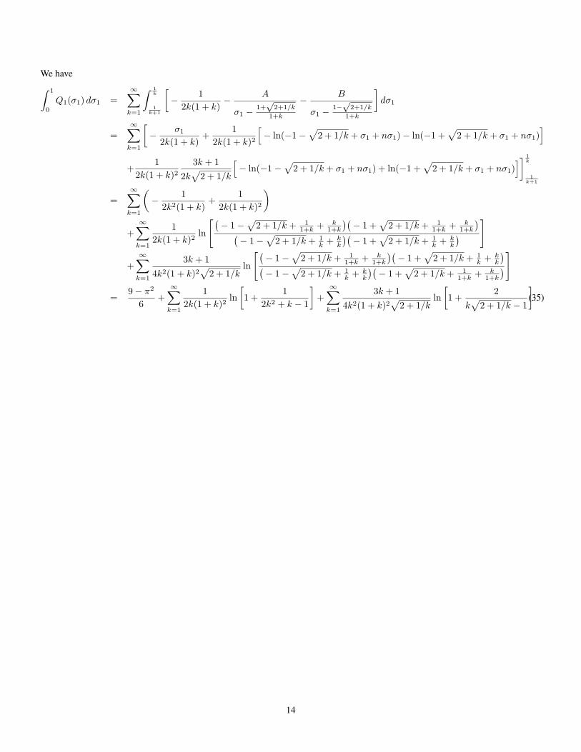
Integral∫ 1

0Q1(σ1) dσ1 (with Q1 as in eq. 24): To obtain

∫ 1

0Q1(σ1) dσ1, we first note that for any integer k ≥ 1, ⌈σ−1

1 ⌉ = k + 1

when σ1 ∈ [ 1k+1 ,

1k ). We have

∫ 1

0

Q1(σ1) dσ1 =∞∑k=1

∫ 1k

1k+1

σ21

−2k(1 + k)σ21 + 4kσ1 + 2

dσ1

=∞∑k=1

∫ 1k

1k+1

[− 1

2k(1 + k)− 2kσ1 + 1

2k(1 + k)(k(1 + k)σ21 − 2kσ1 − 1)

]dσ1.

The second term can be decomposed, defining

A =1 + 3k+1

2k√

2+1/k

2k(1 + k)2and B =

1− 3k+1

2k√

2+1/k

2k(1 + k)2.

13

We have∫ 1

0

Q1(σ1) dσ1 =∞∑k=1

∫ 1k

1k+1

[− 1

2k(1 + k)− A

σ1 −1+

√2+1/k

1+k

− B

σ1 −1−

√2+1/k

1+k

]dσ1

=∞∑k=1

[− σ1

2k(1 + k)+

1

2k(1 + k)2

[− ln(−1−

√2 + 1/k + σ1 + nσ1)− ln(−1 +

√2 + 1/k + σ1 + nσ1)

]+

1

2k(1 + k)23k + 1

2k√

2 + 1/k

[− ln(−1−

√2 + 1/k + σ1 + nσ1) + ln(−1 +

√2 + 1/k + σ1 + nσ1)

]] 1k

1k+1

=∞∑k=1

(− 1

2k2(1 + k)+

1

2k(1 + k)2

)

+∞∑k=1

1

2k(1 + k)2ln

[(− 1−

√2 + 1/k + 1

1+k + k1+k

)(− 1 +

√2 + 1/k + 1

1+k + k1+k

)(− 1−

√2 + 1/k + 1

k + kk

)(− 1 +

√2 + 1/k + 1

k + kk

) ]

+∞∑k=1

3k + 1

4k2(1 + k)2√

2 + 1/kln

[(− 1−

√2 + 1/k + 1

1+k + k1+k

)(− 1 +

√2 + 1/k + 1

k + kk

)(− 1−

√2 + 1/k + 1

k + kk

)(− 1 +

√2 + 1/k + 1

1+k + k1+k

)]

=9− π2

6+

∞∑k=1

1

2k(1 + k)2ln

[1 +

1

2k2 + k − 1

]+

∞∑k=1

3k + 1

4k2(1 + k)2√2 + 1/k

ln

[1 +

2

k√2 + 1/k − 1

].(35)

14