THE RASCH MODEL FOR TEST CONSTRUCTION AND PERSON MEASUREMENT

Benjamin D. Wright

University of Chicago

Prepared for

Fifth Annual Conference and Exhibition

on Measurement and Evaluation

March 14, 1978

Office of the Los Angeles County Superintendent of Schools

Division of Program Evaluation, Research and Pupil Services

Latent trait models for educational measurement are

conceptual inventions that claim to specify what happens

when a person takes a test item. To be worth its salt, a

model must define the supposed causes of the observed response,

direct how to estimate these causes and determine how well

the supposition fits the situation.

Of all the models proposed for item calibration and

person measurement, the Rasch model is the easiest to under-

stand and the easiest to use. Its hypothesized causes are

one ability parameter for each person and one difficulty

parameter for each item. These parameters represent the

relative positions of persons and items on the single latent

variable which they share. They determine the probability of

any particular person succeeding on any particular item.

HOW THE RASCH MODEL WORKS

Understanding the Model

The way these parameters, call them $ v for the ability

of person v and S i for the difficulty of item i, are combined

by the Rasch model is through their difference v ).

This difference governs the probability of what is supposed

to happen when person v pits his ability against the difficulty

of item i. Since this difference can range from minus infinity

to plus infinity, but the probability must stay between zero

and one, the difference is applied as an exponent in

-1-

-2-

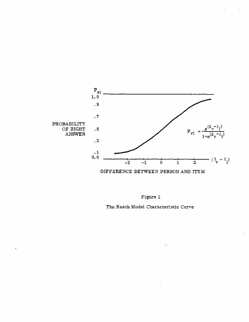
vi ) e and this exponential expression is brought between

ca -5) ($-5) 17 17 zero and one by the ratio e /[1 + e ] which is

the Rasch probability for a right answer (Rasch 1960, 62-126;

1966a; 1966b; Wright, 1968). Figure 1 is a picture of the

way this probability P vi depends on the difference between

person ability $ v and item difficulty S i . Table 1 gives

examples of this relationship.

(Figure 1 and Table 1)

When person v is smarter than item i is difficult,

then (3v

is more than S , , their difference is positive and the _- 1

person's probability of success on item i is greater than one

half. The more the person's ability surpasses the item's

difficulty, the greater this positive difference and the

nearer his probability of success comes to one. But when

the item is too hard for the person, then 13v

is less than S i ,

their difference is negative and the person's probability of

success is less than one half. The more the item overwhelms

the person, the greater this negative difference becomes and

the nearer his probability of success comes to zero.

When we vary person abilities for an item, we have

an item characteristic curve, i.e., a picture of the way the

probability for success on that item changes as persons change

in ability. When we vary item difficulties for a person we

PROBABILITY OF RIGHT

ANSWER

DIFFERENCE BETWEEN PERSON AND ITEM

Figure 1

The Rasch Model Characteristic Curve

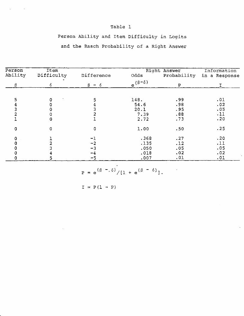
Table 1

Person Ability and Item Difficulty in Logits

and the Rasch Probability of a Right Answer

Person Item Right Answer Information Ability Difficulty Difference Odds Probability in a Response

e °-6) 13, (5 $ - 6 P I

5 0 " 5 148. .99 .01 4 0 4 54.6 .98 .02 3 0 3 20.1 .95 .05 2 0 2 7.39 .88 .11 1 0 1 2.72 .73 .20

0 0 0 1.00 .50 .25

0 1 -1 .368 .27 .20 0 2 -2 .135 .12 .11 0 3 -3 .050 .05 .05 0 4 -4 .018 .02 .02 0 5 -5 .007 .01 .01

•

P = e (8 -.(S) /(1 + e (8 6)l.

I = P(1 - P)

-3-

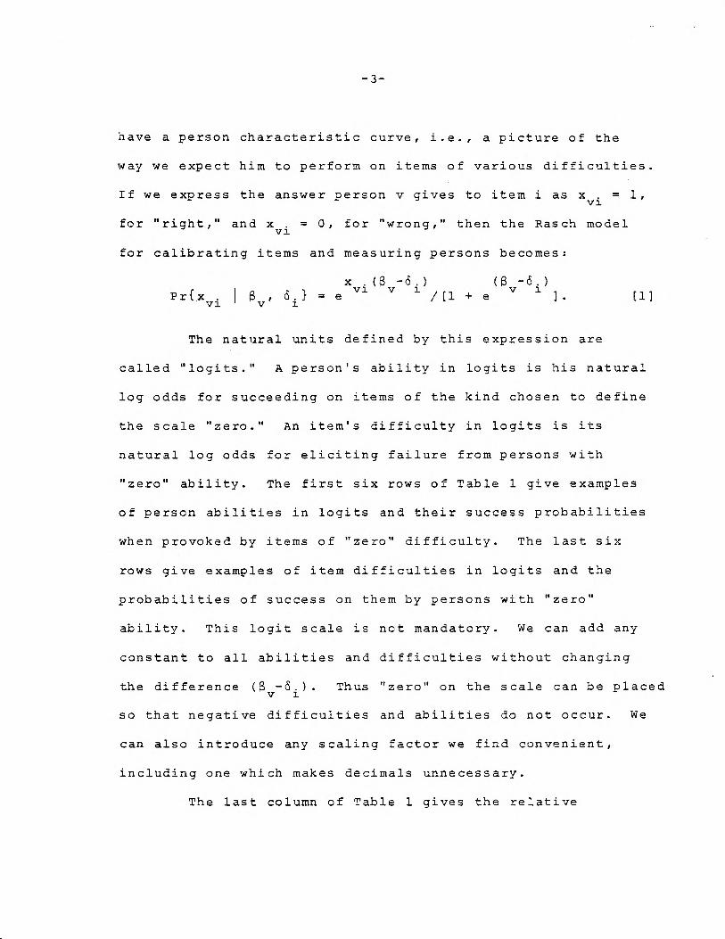
have a person characteristic curve, i.e., a picture of the

way we expect him to perform on items of various difficulties.

If we express the answer person v gives to item i as x vi = 1,

for "right," and xvi

= 0, for "wrong," then the Rasch model

for calibrating items and measuring persons becomes:

x .($ -6) vi v i (f3 v-6 i ) Pr{xvi I v , S i } = e /[1 + e • [1]

The natural units defined by this expression are

called "logits." A person's ability in logits is his natural

log odds for succeeding on items of the kind chosen to define

the scale "zero." An item's difficulty in logits is its

natural log odds for eliciting failure from persons with

"zero" ability. The first six rows of Table 1 give examples

of person abilities in logits and their success probabilities

when provoked by items of "zero" difficulty. The last six

rows give examples of item difficulties in logits and the

probabilities of success on them by persons with "zero"

ability. This logit scale is not mandatory. We can add any

constant to all abilities and difficulties without changing

the difference (a 1, -(5 i ). Thus "zero" on the scale can be placed

so that negative difficulties and abilities do not occur. We

can also introduce any scaling factor we find convenient,

including one which makes decimals unnecessary.

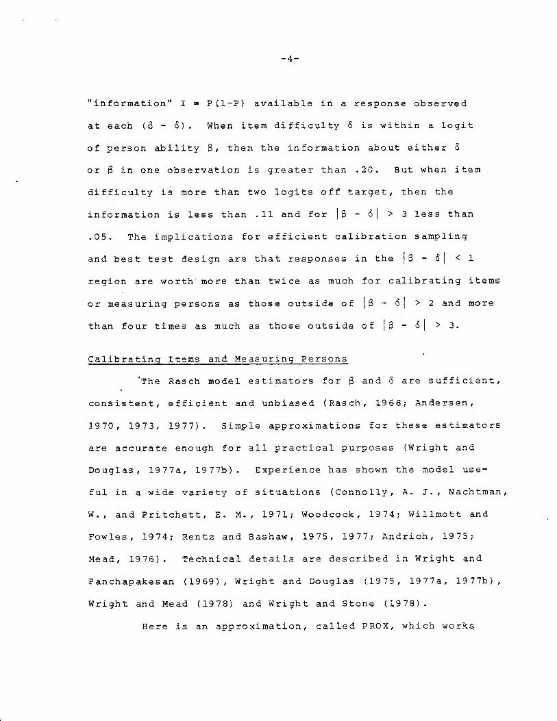
The last column of Table 1 gives the relative

-4-

"information" I = P(1-P) available in a response observed

at each (6 - 6). When item difficulty 6 is within a logit

of person ability 6, then the information about either 6

or 6 in one observation is greater than .20. But when item

difficulty is more than two logits off target, then the

information is less than .11 and for 16 - 61 > 3 less than

.05. The implications for efficient calibration sampling

and best test design are that responses in the 16 - 61 < 1

region are worth' more than twice as much for calibrating items

or measuring persons as those outside of 16 - 61 > 2 and more

than four times as much as those outside of 16 - 61 > 3.

Calibrating Items and Measuring Persons

The Rasch model estimators for 6 and 6 are sufficient,

consistent, efficient and unbiased (Rasch, 1968; Andersen,

1970, 1973, 1977). Simple approximations for these estimators

are accurate enough for all practical purposes (Wright and

Douglas, 1977a, 1977b). Experience has shown the model use-

ful in a wide variety of situations (Connolly, A. J., Nachtman,

W., and Pritchett, E. M., 1971; Woodcock, 1974; Willmott and

Fowles, 1974; Rentz and Bashaw, 1975, 1977; Andrich, 1975;

Mead, 1976). Technical details are described in Wright and

Panchapakesan (1969), Wright and Douglas (1975, 1977a, 1977b),

Wright and Mead (1978) and Wright and Stone (1978).

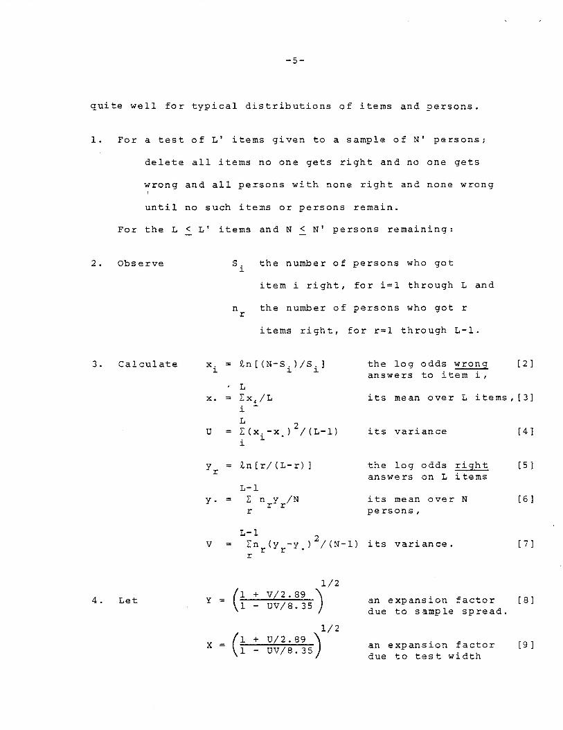
Here is an approximation, called PROX, which works

-5-

quite well for typical distributions of items and persons.

1. For a test of L' items given to a sample of N' persons;

delete all items no one gets right and no one gets

wrong and all persons with none right and none wrong

until no such items or persons remain.

For the L < L' items and N < N' persons remaining:

2. Observe Si

the number of persons who got

item i right, for i=1 through L and

nr

the number of persons who got r

items right, for r=1 through L-1.

3. Calculate xi = Zn[(N-S

i)/S] the log odds wrong [2]

answers to item i, • L

x. = Exi /L its mean over L items,[3]

U = E(xi -x • )2/(L-1) its variance [4]

y = Zn[r/(L-r)] the log odds right [5] answers on L items

L-1 y. = E n r

y r/N its mean over N [6]

r persons,

L-I V = En r (y r-y

. )2/(N-1) its variance. [7]

1/2 (1 + V/2.1 - UV/8

8.935)

4. Let Y - an expansion factor [8] due to sample spread.

1/2

X (1 - UV/8.1 + U/2.89

35 )

- an expansion factor [9] due to test width

-6-

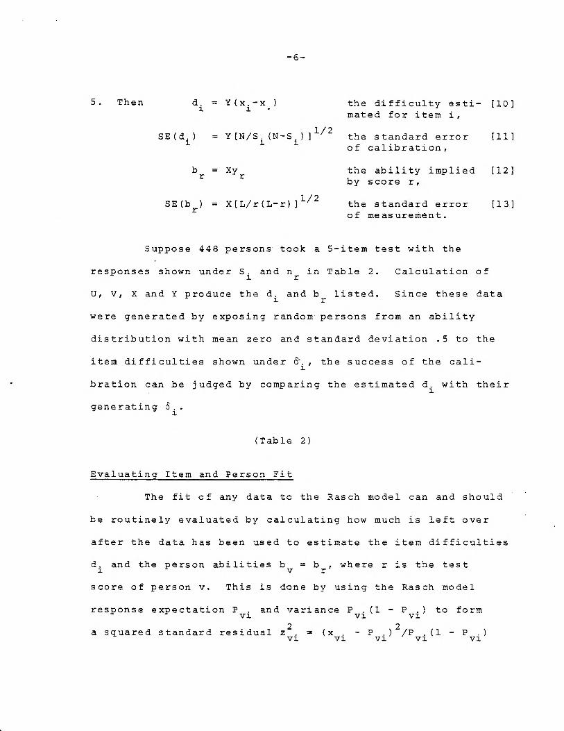
5. Then d, = Y(x.-x ) the difficulty esti- [10] 1 mated for item i,

SE(d.) = Y[N/Si (N-S )] 1/2 the standard error

[11] 1

of calibration,

br

= Xyr the ability implied [12]

by score r,

SE(br) = X[L/r(L-r)] 1"2 the standard error [13]

of measurement.

Suppose 448 persons took a 5-item test with the

responses shown under Si

and nr in Table 2. Calculation of

U, V, X and Y produce the d i and b r listed. Since these data

were generated by exposing random persons from an ability

distribution with mean zero and standard deviation .5 to the

item difficulties shown under &i'

the success of the cali-

bration can be judged by comparing the estimated d i with their

generating S i .

(Table 2)

Evaluating Item and Person Fit

The fit of any data to the Rasch model can and should

be routinely evaluated by calculating how much is left over

after the data has been used to estimate the item difficulties

d i and the person abilities by

= b r , where r is the test

score of person v. This is done by using the Rasch model

response expectation Pvi

and variance Pvi (1-

P vi ) to form

2 a squared standard residual z

vi = (x

vi -

Pvi)2/Pvi(1 - P

vi)

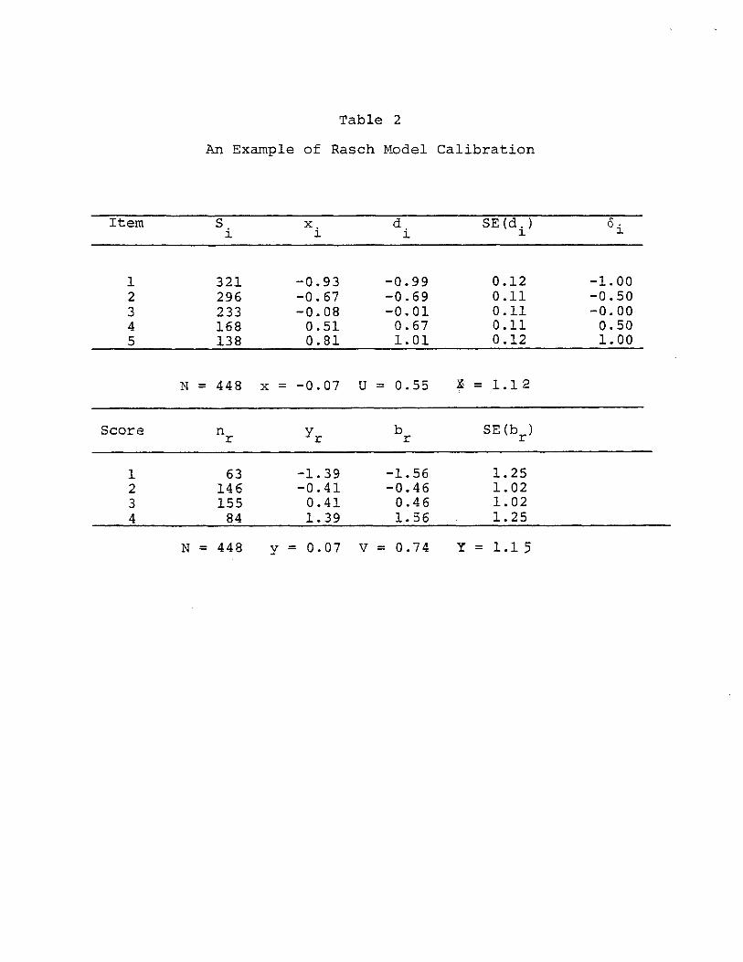
Table 2

An Example of Rasch Model Calibration

Item S x. d SE(d.) S i i 1 i 1

1 321 -0.93 -0.99 0.12 -1.00 2 296 -0.67 -0.69 0.11 -0.50 3 233 -0.08 -0.01 0.11 -0.00 4 168 0.51 0.67 0.11 0.50 5 138 0.81 1.01 0.12 1.00

N = 448 x = -0.07 U = 0.55 X = 1.12

Score nr Yr br

SE(br )

1 63 -1.39 -1.56 1.25 2 146 -0.41 -0.46 1.02 3 155 0.41 0.46 1.02 4 84 1.39 1.56 1.25

N = 448 y = 0.07 V = 0.74 Y = 1.15

-7-

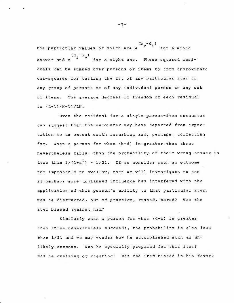
(b-d) v the particular values of which are e for a wrong

(di v -b)

answer and e for a right one. These squared resi-

duals can be summed over persons or items to form approximate

chi-squares for testing the fit of any particular item to

any group of persons or of any individual person to any set

of items. The average degrees of freedom of each residual

is (L-1)(N-1)/LN.

Even the residual for a single person-item encounter

can suggest that the encounter may have departed from expec-

tation to an extent worth remarking and, perhaps, correcting

for. When a person for whom (b-d) is greater than three

nevertheless fails, then the probability of their wrong answer is

less than 1/(1+e3 ) = 1/21. If we consider such an outcome

too improbable to swallow, then we will investigate to see

if perhaps some unplanned influence has interfered with the

application of this person's ability to that particular item.

Was he distracted, out of practice, rushed, bored? Was the

item biased against him?

Similarly when a person for whom (d-b) is greater

than three nevertheless succeeds, the probability is also less

than 1/21 and we may wonder how he accomplished such an un-

likely success. Was he specially prepared for this item?

Was he guessing or cheating? Was the item biased in his favor?

-8-

WHAT THE RASCH MODEL DOES

Item Calibration Can Be Sample-Free

When the Rasch model is used to govern measurement,

then the unweighted sum of right answers given by persons

taking an item can be used to estimate sample-free item

calibrations. The traditional index of item difficulty,

proportion right in some calibrating sample, varies with the

sample's ability distribution, e.g., high for smart samples,

low for dumb ones. To obtain a sample-free calibration we

must adjust the sample-bound item score for the influence of

sample ability.

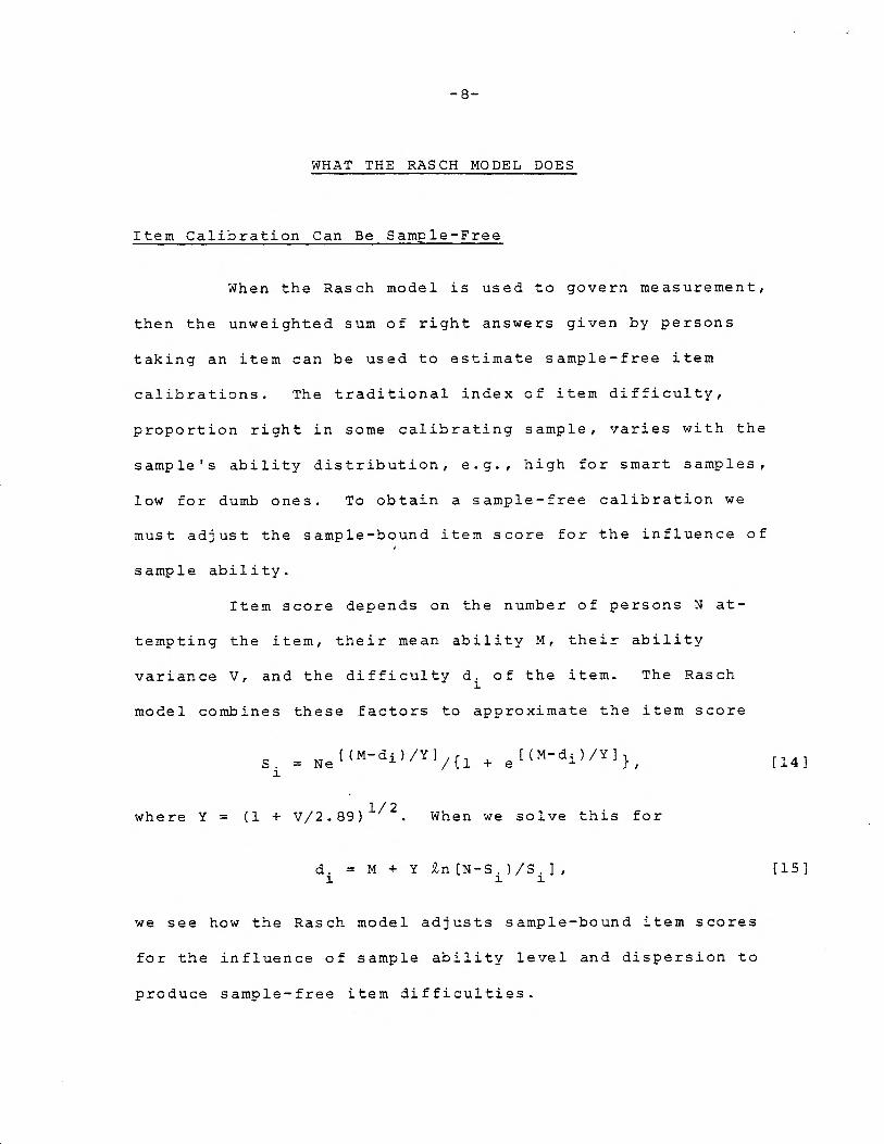
Item score depends on the number of persons N at-

tempting the item, their mean ability M, their ability

variance V, and the difficulty di of the item. The Rasch

model combines these factors to approximate the item score

[(M-di)/Y] r [(M- di)/Yll Si

= Ne /t1 + e (14]

where Y = (1 + V/2.89)1/2 . When we solve this for

di = M + Y Zn[N-S

i)/S

i], [15]

we see how the Rasch model adjusts sample-bound item scores

for the influence of sample ability level and dispersion to

produce sample-free item difficulties.

-9-

Item Validity Can be Evaluated by a Chi-Square Test of Item Fit

The validity of any item with respect to any sample

of persons and even to a particular person can be evaluated

explicitly by fitting the Rasch model, calculating the dif-

ference between the observed data and the values expected by

the model and examining these residuals. While a single im-

probable residual does not determine whether the trouble lies

in the person or the item, when squared residuals are summed

over persons for an item, the magnitude of their sum provides

a chi-square test of the item's validity (Wright and Panchapakesan,

1969; Wright, Mead, and Draba, 1976; Mead, 1976).

If an item is thought to be biased with sex or culture,

then its unsquared residuals, -e(b-d)/2 for a wrong answer and

(d-b)/2 for a right answer, can be regressed over persons

on indicators of these background variables to see if object-

ive signs of bias are observable. Since items discovered to

be biased can be deleted from persons' responses without

spoiling estimates of their ability, we can correct for item

bias in a test without losing the information available from

items which are not biased.

Item Reliability Can Be Estimated By a Standard Error of Calibration

The Rasch model provides an estimate of the reliability

-10-

if each item calibration. This standard error of item dif-

ficulty depends on how large the calibrating sample is and

on how central the sample is to the item. It is well ap-

proximated by 2.5/N1/2

logits where N is the calibration

sample size, and 2.5 is a compromise value for the effect of

sample relevance which varies from 2 when the sample is en-

tirely centered on the item through 3 as the sample proportion

of right answers goes below 15% or above 85% (Wright and

Douglas, 1975, 16-18, 34).

Item Banks Can Equate All Possible Tests

When items are constructed and administered so that

their performance approximates the Rasch model, then item

difficulties estimated from a variety of calibrating samples

can be shifted easily onto a single common scale. The re-

sulting commonly calibrated items form an item bank from which

can be drawn any subset of items thought to be appropriate to

make a best test (Choppin, 1968, 1976; Willmott and Fowles,

1974, 46-51). Since the measures implied by scores on all

such tests are automatically equated, the problem of test

equating for all possible tests drawn from the bank is com-

pletely solved, once and for all (Rentz and Bashaw, 1975, 1977).

Tests are usually equated by giving them to a common

sample of persons and connecting them by their simultaneous

score distributions. All the items on a pair of tests administered

-11-

this way can be calibrated onto a common Rasch scale by con-

sidering the pair as one long test. A more economical method

for building an item bank, however, is to embed links of 10

to 20 common items in pairs of otherwise different tests.

Each test can then be taken by its own sample of persons so

that no person need take more than one test. All items in all

tests can be connected through the network of links.

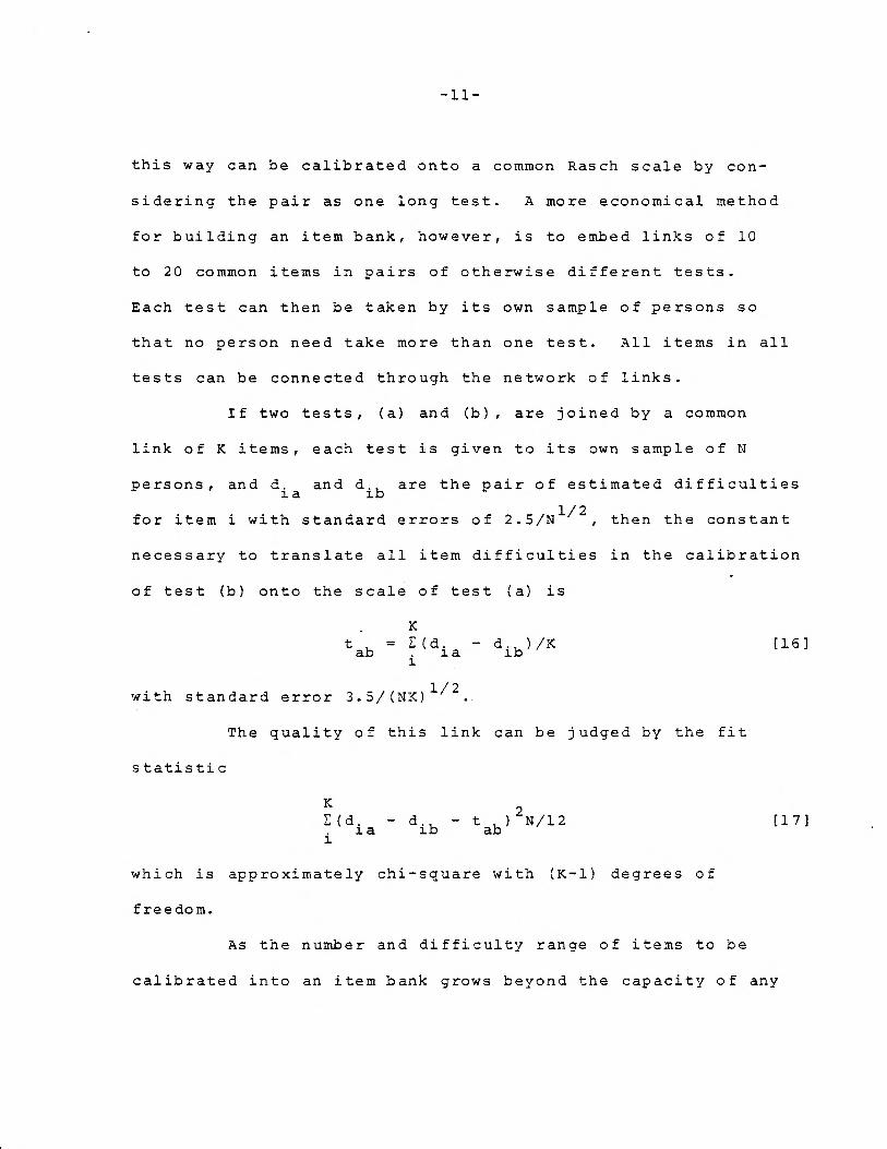
If two tests, (a) and (b), are joined by a common

link of K items, each test is given to its own sample of N

persons, and dia

and dib

are the pair of estimated difficulties

for item i with standard errors of 2.5/N1/2

, then the constant

necessary to translate all item difficulties in the calibration

of test (b) onto the scale of test (a) is

K tab

= E(dia

- dib

)/K [16]

with standard error 3.5/(NK)1/2

The quality of this link can be judged by the fit

statistic

K E(dia d

ib - tab) 2N/12 [17]

which is approximately chi-square with (K-1) degrees of

freedom.

As the number and difficulty range of items to be

calibrated into an item bank grows beyond the capacity of any

-12-

one person, items can be distributed over a network of inter-

linking tests and the estimated translations checked against

one another for coherence (Doherty and Forster, 1976; Ingebo,

1976).

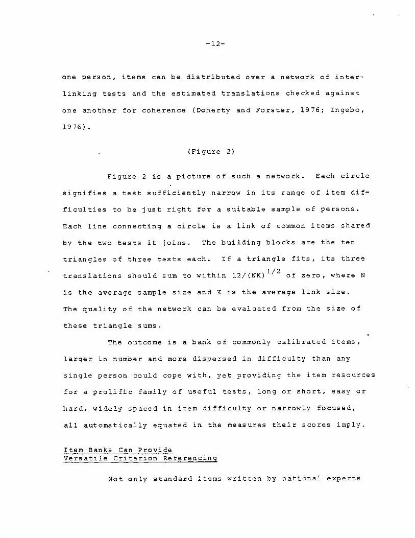
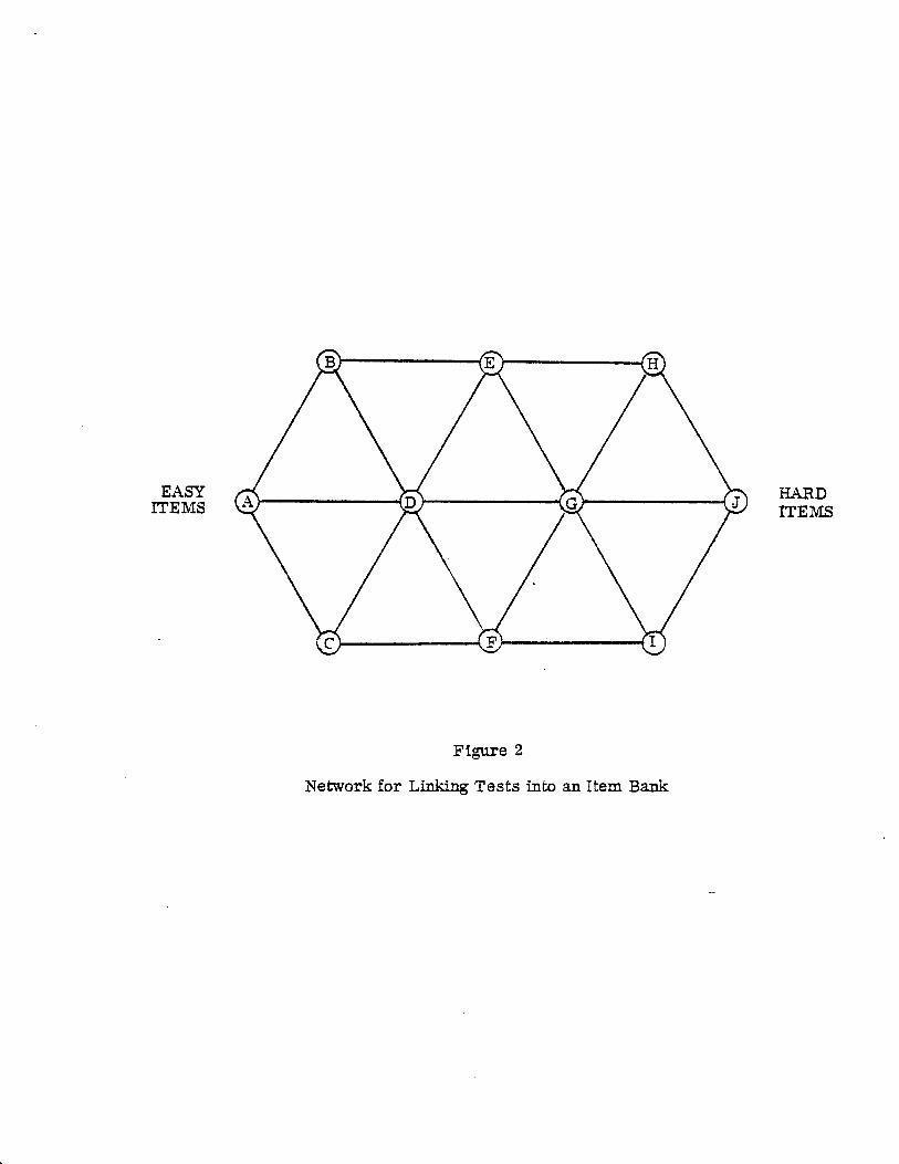
(Figure 2)

Figure 2 is a picture of such a network. Each circle

signifies a test sufficiently narrow in its range of item dif-

ficulties to be just right for a suitable sample of persons.

Each line connecting a circle is a link of common items shared

by the two tests it joins. The building blocks are the ten

triangles of three tests each. If a triangle fits, its three

translations should sum to within 12/(NK)1/2 of zero, where N

is the average sample size and K is the average link size.

The quality of the network can be evaluated from the size of

these triangle sums.

The outcome is a bank of commonly calibrated items,

larger in number and more dispersed in difficulty than any

single person could cope with, yet providing the item resources

for a prolific family of useful tests, long or short, easy or

hard, widely spaced in item difficulty or narrowly focused,

all automatically equated in the measures their scores imply.

Item Banks Can Provide Versatile Criterion Referencing

Not only standard items written by national experts

EASY ITEMS

HARD ITEMS

Figure 2

Network for Linking Tests into an Item Bank

-13-

but special items written by local users can be calibrated

into the same bank. The decisions for keeping or dropping

items, whether nationally sanctioned or locally inspired,

can be made on entirely objective grounds. If an item fits,

it is kept. If there are milestone events like grades, pro-

motions and graduations, then mastery of these criteria can

be introduced into the analysis along with performance on

ordinary items and each criterion can be calibrated into the

bank just like any item. Then 'every measurement mode will

deliver that person's standing with respect to all calibrated

criteria. Criterion referencing can be done with any items

in the bank.

The investigation of what kinds of items fit a bank

and what kinds donot makes possible a detailed analysis of — —

the latent variable's operational definition. Any hypothesis

about the nature of the variable which can be expressed in

observable events can be empirically investigated by attempt-

ing to calibrate these "challenge" events into the bank and

observing how well they fit.

Item Banks Can Expedite Norm Referencing

Norms are no more fundamental to the calibration of

items than distributions of height are to the ruling of yard-

sticks. But once a bank is established, it is very useful to

learn the normative characteristics of the variable it defines.

-14-

To norm a variable, rather than a test, we need only use

enough items to estimate the norm statistics. The mean and

standard deviation of any cell in our sampling plan can be

estimated rather well from a random sample of 100 persons

taking a norming test of 10 items (Wright, 1977) . Once the

variable is normed, all possible scores from all possible

tests drawn from the bank are automatically norm referenced.

Person Measurement Can Be Test-Free

When two persons earn the same score we usually

take their test performances to be equivalent. When we do

not care which items produce a score, we are practicing

"item-free" measurement. The Rasch model shows how item-free

measurement within a test leads, without additional assumptions,

to test-free measurement within a bank of calibrated items.

This is done by removing test differences in item difficulty

so that what is left is a test-free person measure on the

scale defined by the bank calibrations.

Person score depends on the number of items L in

the test, their mean difficulty level H, their difficulty

variance U and the ability b r of the person scoring r. The

Rasch model combines these factors to approximate the person

score

r = L e 1 + e [(b r - H)/X) /{1 [(b r - H)/X],

[18]

1/2 where X = (1 + U/2.89)

-15-

When we solve this equation for

br = H + X Zn[r/(L - r)] [19]

we see how the Rasch model adjusts test-bound person scores

for test difficulty level and spread to produce test-free

person measures.

Measurement Validity Can Be Evaluated by a Chi-Square Test of Person Fit

When a person takes a test we cannot be sure he will

work as intended. We try to give him enough time, to choose

items relevant to his ability level and to motivate him so

that he will work with all his ability on the answer to every

item. But we know that some persons under some circumstances

nevertheless render flawed performances. Test scores are

bound to be influenced by guessing, sleeping, practice and

speed. We must detect these influences and, where possible,

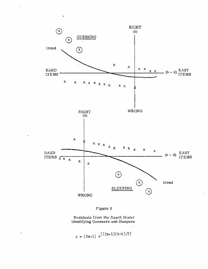
correct for them. If guessing on difficult items or sleeping

on easy items influences a person's responses, then plotting

his response residuals -e(b-d)/2 for a wrong answer and

(d-b)/2 for a right one against item difficulty will bring

that out. Figure 3 shows these residuals plotted against

the estimated differences (b - d) for typical guessers and

sleepers.

(Figure 3)

HARD ITEMS

_ d EASY ITEMS

GUESSING

- d) EASY (b ITEMS

HARD ITEMS

SLEEPING

Figure 3

Residuals from the Rasch Model Identifying Guessers and Sleepers

-16-

If lack of practice affects early items or lack of speed

affects late ones, plotting residuals against item posi-

tion will bring that out.

These analyses are available for each person. No

assumption need be made that everyone guesses, sleeps,

fumbles or plods. Those possibilities can be evaluated

on an individual basis and each person's responses edited

to remove or correct the disturbance he actually manifests.

Another source of person misfit is item bias. If

the test of a math item is difficult to read, then poor

readers will find it biased against the expression of their

math ability. If a reading item uses special vocabulary,

then it will be biased against the expression of reading

ability among the unexposed. The analysis of residu.ils puts

the detection of item bias on a sound footing and provides

a quantitative basis for correcting it (Wright, Mead, and

Draba, 1976).

Measurement Reliability Can Be Estimated by a Standard Error of Measurement

The precision with which a particular person is

measured by a test depends on how many items he takes and

how relevant these items are to his ability. When the test's

difficulty level is within a logit or so of the person's

ability then item relevance plays a minor role and the standard

-17-

error of measurement can be approximated by 2.5/L 1/2, where

L is the number of items taken and 2.5 is a compromise value

for the test relevance coefficient (Wright and Douglas, 1975,

16-18, 34).

Best Test Design Becomes Simple

With an item bank to draw upon and a model to

specify how a person and an item are supposed to interact

it becomes easy to design and construct the best possible

test for any measurement situation (Wright and Douglas, 1975,

1-18). All reasonable possibilities for target distributions

and test shapes are covered by the following simple procedure

(Wright and Douglas, 1975, 26-41).

1. Guess target location M and uncertainty S as

well as possible. If outer boundaries are used to specify

the target, relate them to M and S by letting the lower

boundary define M-2S and the upper boundary define M+2S.

2. Design a - test centered at M and spread evenly

over the range M-2S to M+2S, with enough items between to

produce a test length of L = 6/SEM2, where SEM is the de-

sired standard error of measurement.

3. Select from the item bank the best available

items to fulfill this design and use the mean and the range

of the obtained item difficulties to describe the height

h and width w of the resulting test.

-18-

This test is as good for all practical purposes as

any other test of equal length which might be constructed to

measure the anticipated target. One all-purpose table of

within test measures x fw for relative scores of f = r/.L on

tests of width w and height h can be used to convert any

score r on any such test into a test-free measure of person

ability b f through the relation b f = h + x fw . Standard errors

can be approximated with 2.5/L1/2 . No further calculations

are ever needed to convert a test-bound score to a test-free

measure (Wright and Douglas, 1975, 32-35).

Tailored Testing Becomes Easy

The construction of a bank of calibrated items makes

the implementation of tailored-testing easy. The uniformity

of measurement precision between 25% and 75% right answers

shows that we need only bring items to within a logit of

their target for optimal tailoring. In many situations the

grade placement of the target group or pupil and the variable's

grade norms will be sufficient to determine an appropriate

selection of items. Typical within grade standard deviations

are about one logit. When this is so, even a rough idea of

a pupil's within grade quartile provides more than enough

information to design a best test for that pupil.

If placement tailoring is inconvenient, then per-

formance tailoring can be accomplished with a self-scoring

-19-

pilot test of 5 to 10 items spread out in difficulty to

cover the worst possible target. Pupils can use their number

right to guide themselves into a second test of 40 to 50

items focused on the ability region implied by their pilot

score (Forbes, 1976).

If an even more individualized procedure is desired,

the pupil can be given a booklet of 100 or so items arranged

in uniformly increasing difficulty and asked to find his own

working level. His tailored testing begins when he finds

items hard enough to interest him but easy enough to handle.

He works forward into more difficult items until time is up

or the increasing difficulty overwhelms him. If time remains,

he goes back to his first item and works backward into easier

items. The self-tailored test on which this pupil is measured

is the continuous segment of items from the easiest through

the most difficult he attempts. The procedure is self-adapting

to individual variations in speed and level of productive

challenge. The individualized test segments which result are

handled by using a self-scoring form to record the sequence

number of the easiest and hardest items tried and the number

of right answers. These three statistics can find the cor-

responding measure and its standard error in a one page table

calculated to fit with the booklet of items.

References

Andersen, E. B. Asymptotic properties of conditional maximum

likelihood estimators, Journal of the Royal Statisti-

cal Society. 1970, 32, 283-301.

Andersen, E. B. A Goodness of fit test for the Rasch model.

Psychometrika, 1973, 38, 123-140.

Andersen, E. B. Sufficient statistics and latent trait models.

Psychometrika, 1977, 42, 69-81.

Andrich, D. The Rasch multiplicative binomial model: applica-

tions to attitude data. Research Report No. 1,

Measurement and Statistics Laboratory, Department of

Education, University of Western Australia, 1975.

Choppin, B. An item bank using sample-free calibration.

Nature, 1968, 219 (51561, 870-872.

Choppin, B. Recent developments in item banking. In Advances

in Psychological and Educational Measurement. New

York: Wiley, 1976.

Connolly, A. J., Nachtman, W., and Pritchett, E. M. Keymath:

Diagnostic Arithmetic Test. Circle Pines, Minn.:

American Guidance Service, 1971.

Doherty, V. W., and Forster, F. Can Rasch scaled scores be

predicted from a calibrated item pool? American Edu-

cational Research Association, San Francisco, 1976.

-20-

-21-

Forbes, D. W. The use of Rasch logistic scaling procedures

in the development of short multi-level arithmetic

achievement tests for public school measurement.

American Educational Research Association, San

Francisco, 1976.

Ingebo, G. How to link tests to form an item pool. American

Educational Research Association, San Francisco, 1976.

Mead, R. J. Assessing the fit of data to the Rasch model

through analysis of residuals. Doctoral dissertation,

University of Chicago, 1976.

Rasch, G. Probabilistic Models for some. Intelligence and

Attainment Tests. Copenhagen, Denmark: Danmarks

Paedogogiske Institut, 1960. ,

Rasch, G. An individualistic approach to item analysis. In

P. F. Lazarsfeld and N. W. Henry (Eds.), Readings in

Mathematical Social Science. Chicago: Science Research

Associates, 1966a, 89-108.

Rasch, G. An item analysis which takes individual differences

into account. British Journal of Mathematical and

Statistical Psychology, 1966b, 19 (1), 49-57.

Rasch, G. A mathematical theory of objectivity and its conse-

quences for model construction. Report from European

Meeting on Statistics, Econometrics and Management

Sciences, Amsterdam, 1968.

-22-

Rentz, R. R., and Bashaw, W. L. Equating Reading Tests with

the Rasch Model. Athens, Georgia: Educational Re-

source Laboratory, 1975.

Rentz, R. R., and Bashaw, W. L. The national reference scale

for reading: An application of the Rasch model.

Journal of Educational Measurement, 1977, 14, 161-180.

Wilmott, A., and Fowles, D. The Objective Interpretation of

Test Performance: The Rasch Model Applied. Atlantic

Highlands, N.J.: NFER Publishing Co., Ltd., 1974.

Woodcock, R. W. Woodcock Reading Mastery Tests. Circle Pines,

Minnesota: American Guidance Service, 1974.

Wright, B. D. Sample-free test calibration and person measure-

ment. In Proceedings of the 1967 Invitational Con-

ference on Testing Problems. Princeton, N.J.: Edu-

cational Testing Service, 1968, 85-101.

Wright, B. D. Solving measurement problems with the Rasch

model. Journal of Educational Measurement, 1977, 14,

97-116.

Wright, B. D., and Douglas, G. A. Best test design and self-

tailored testing. Research Memorandum No. 19,

Statistical Laboratory, Department of Education,

University of Chicago, 1975.

Wright, B. D., and Douglas, G. A. Best procedures for sample-

free item analysis. Applied Psychological Measurement,

1, 1977a, 281-295.

-2 3-

Wright, B. D., and Douglas, G. A. Conditional versus

unconditional procedures for sample-free item analysis.

Educational and Psychological Measurement, 37, 1977b,

573-586.

Wright, B. D., and Mead, R. J. BICAL: Calibrating rating

scales with the Rasch model. Research Memorandum

No. 23A, Statistical Laboratory, Department of Edu-

cation, University of Chicago, 1978.

Wright, D. B. , Mead, R. J. , and Draba, R. Detecting and cor-

recting test item bias with a logistic response model.

Research Memorandum No. 22, Statistical Laboratory,

Department of Education, University of Chicago, 1976.

Wright, B. D., and Panchapakesan, N. A procedure for sample-

free item analysis. Educational and Psychological

Measurement, 1969, 29, 23-48.

Wright, B. D., and Stone, M. H. Best Test Design: A Handbook

for Rasch Measurement. Palo Alto: The Scientific

Press, 1978.