Embed Size (px)
Citation preview
The Quantitative Importance of Openness in
Development
Wenbiao Cai, B. Ravikumar and Raymond G. Riezman
Department of Economics Working Paper Number: 2013-02
THE UNIVERSITY OF WINNIPEG
Department of Economics
515 Portage Avenue
Winnipeg, R3B 2E9
Canada
This working paper is available for download at:
http://ideas.repec.org/s/win/winwop.html
The Quantitative Importance of Openness in
Development
Wenbiao Cai∗ B. Ravikumar† Raymond G. Riezman‡
August 2013
Abstract
This paper deals with a classic development question: how can the process of economicdevelopment – transition from stagnation in a traditional technology to industrializationand prosperity with a modern technology – be accelerated? Lewis (1954) and Rostow(1956) argue that the pace of industrialization is limited by the rate of capital formationwhich in turn is limited by the savings rate of workers close to subsistence. We arguethat access to capital goods in the world market can be quantitatively important inspeeding up the transition. We develop a parsimonious open-economy model wheretraditional and modern technologies coexist (a dual economy in the sense of Lewis(1954)). We show that a decline in the world price of capital goods in an open economyincreases the rate of capital formation and speeds up the pace of industrializationrelative to a closed economy that lacks access to cheaper capital goods. In the longrun, the investment rate in the open economy is twice as high as in the closed economyand the per capita income is 23 percent higher.
JEL codes: O11, F43, O14
Keywords: Openness; Industrialization; Capital formation; Relative price of investment
We thank Manish Pandey and participants at the 2013 Canadian Economics Association meeting forhelpful comments. We also thank Judith Ahlers for editorial assistance. The views expressed in this articleare those of the authors and do not necessarily reflect the views of the Federal Reserve Bank of St. Louis orthe Federal Reserve System.
∗Department of Economics, University of Winnipeg. [email protected]†Research Division, Federal Reserve Bank of Saint Louis. [email protected]‡Department of Economics, University of Iowa. [email protected]
1
1 Introduction
One of the most fundamental questions in development economics is how a poor country with
a stagnant economy makes the transition to a modern, growing, and prosperous country.
Lewis (1954) and Rostow (1956) start with the observation that the industrialization process
is capital intensive and that the absorption of labor into the industrialized sector is limited
by the amount of capital. For developing countries the main source of funds for capital
formation is domestic savings. Both Lewis and Rostow also observe that these countries
have an abundance of unskilled labor that typically has very low productivity. Workers in
this situation at best earn subsistence wages and hence there is little or no surplus available
for saving. The lack of saving limits the rate of capital formation and, hence, the rate of
absorption of labor into the industrialized sector. Thus, the transition from being a poor
country to a prosperous one is a gradual process.
How can the process of economic development – transition from stagnation to industri-
alization – be accelerated? Nurkse (1958), Ranis and Fei (1961), and Rostow (1960) argue
that the development process can be accelerated by an increase in agricultural productivity.
In their argument, the increase in productivity leads to an increase in surplus that can be
used to boost the rate of capital formation, thereby speeding up development.
While the channel of domestic capital formation might be important for closed economies,
it is not clear whether the limitations on capital formation imposed by this channel are
quantitatively important for open economies. For instance, access to international capital
goods markets could provide more funds for capital formation and act as a catalyst for
economic development. In this paper, we show that openness in the form of access to capital
goods at lower prices increases the rate of capital formation and speeds up the process of
economic development.
In our model, there are two technologies – traditional and modern – for producing a single
consumption good, as in Hansen and Prescott (2002). During the process of development,
both traditional and modern techniques coexist in the economy (i.e., it is a dual economy in
2
the sense of Lewis (1954)). We consider the transition from traditional to modern technology
as the process of industrialization. The traditional technology is a decreasing returns to
scale technology that uses only labor. The modern technology is a constant returns to scale
technology that uses both capital and labor. We embed these two technologies into a simple
open-economy model of capital accumulation.
An important feature of our model is that there are barriers to capital accumulation. In
a closed economy, such barriers distort the price of capital to be higher than that in an open
economy. The high price of capital goods in a closed economy leads to slower capital accu-
mulation. In turn, the absorption of labor from traditional to modern technology is slower
since the absorption is limited by the amount of capital. Hence, economic development in a
closed economy is slow and most of the labor force is employed in the traditional technology.
In the open economy, domestic producers gain access to a continually declining international
price of capital goods. This international access leads to a more rapid rate of capital accu-
mulation. Faster capital accumulation not only fosters income growth, but also accelerates
the absorption of labor into the modern technology.
Table 1 documents the growth of per capita gross domestic product (GDP) and the
price of investment relative to consumption for Korea, China, India, and Taiwan. All of
these countries experienced major trade liberalization at some point in the latter half of
the twentieth century. Table 1 shows that prior to the liberalization, each country exhibits
increasing or steady relative price of investment and relatively modest growth rates. This
contrasts sharply with post-liberalization periods in which there is faster economic growth
along with a steady decline in the relative price of investment. These data suggest a link
between the lower price of investment goods and higher economic growth.
This link leads to our main question: How important was access to cheaper capital for
accelerating the transition from stagnation to industrialization? We show that it is indeed
quantitatively important.
To illustrate the quantitative importance of openness, we use our model and the observed
3
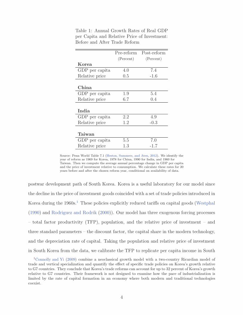
Table 1: Annual Growth Rates of Real GDPper Capita and Relative Price of Investment:Before and After Trade Reform
Pre-reform Post-reform(Percent) (Percent)
Korea
GDP per capita 4.0 7.4Relative price 0.5 -1.6
China
GDP per capita 1.9 5.4Relative price 6.7 0.4
India
GDP per capita 2.2 4.9Relative price 1.2 -0.3
Taiwan
GDP per capita 5.5 7.0Relative price 1.3 -1.7
Source: Penn World Table 7.1 (Heston, Summers, and Aten, 2012). We identify theyear of reform as 1969 for Korea, 1978 for China, 1990 for India, and 1960 forTaiwan. Then we compute the average annual percentage change in GDP per capitaand the price of investment relative to consumption. We calculate these rates for 20years before and after the chosen reform year, conditional on availability of data.
postwar development path of South Korea. Korea is a useful laboratory for our model since
the decline in the price of investment goods coincided with a set of trade policies introduced in
Korea during the 1960s.1 These policies explicitly reduced tariffs on capital goods (Westphal
(1990) and Rodriguez and Rodrik (2000)). Our model has three exogenous forcing processes
– total factor productivity (TFP), population, and the relative price of investment – and
three standard parameters – the discount factor, the capital share in the modern technology,
and the depreciation rate of capital. Taking the population and relative price of investment
in South Korea from the data, we calibrate the TFP to replicate per capita income in South
1Connolly and Yi (2009) combine a neoclassical growth model with a two-country Ricardian model oftrade and vertical specialization and quantify the effect of specific trade policies on Korea’s growth relativeto G7 countries. They conclude that Korea’s trade reforms can account for up to 32 percent of Korea’s growthrelative to G7 countries. Their framework is not designed to examine how the pace of industrialization islimited by the rate of capital formation in an economy where both modern and traditional technologiescoexist.
4
Korea from 1970 to 2007. The calibrated model is able to reproduce the observed secular
decline in the share of the labor force employed in the traditional technology (proxied by the
observed share of the rural population).2 The model is also able to reproduce the increase in
the investment rate.
We then use the calibrated model to measure the quantitative importance of openness for
economic development. We conduct a counterfactual exercise in which the price of investment
does not decline as observed in the data, but instead remains at the pre-reform (1969) level.
We then evaluate the changes to per capita income and the allocation of labor. We find
that had the Korean economy remained closed, per capita income would have reached only
80 percent of its observed level in 2007. Moreover, it would have taken 12 more years to
reach the fraction of labor employed in the modern technology in 2007. The investment rate
increases over time in both open and closed economies, but capital accumulation is more
rapid in the open economy. For instance, the investment rate in the open economy in 2007
is twice that in the closed economy. Stated differently, both open and closed economies
transition from stagnation to industrialization, but the the transition occurs sooner in the
open economy. These results on labor absorption and investment rate are consistent with the
arguments in Lewis (1954) and Rostow (1956) that the pace of industrialization is limited by
the amount of capital.
In our model, the difference between the paths of GDP per capita in the open and closed
economies is due entirely to the difference between the paths of two endogenous variables:
capital stock and the fraction of labor in the modern technology. The difference between
the paths of GDP per capita can be mechanically accounted for as follows. Starting with
the closed economy, we change the share of labor allocated to the modern technology to the
share in the open economy and let the path of capital remain the same as that in the closed
economy. Such a change in the path of labor leaves the GDP per capita in the closed economy
virtually unchanged. This suggests that the difference between the paths of GDP per capita
2In what follows, we associate the traditional technology with rural areas and modern technology withurban areas and treat industrialization and urbanization as synonymous.
5
is accounted for by the difference in the paths of capital. To confirm this, we perform the
reverse mechanical experiment: Starting with the closed economy, we change the path of
capital to the one in the open economy and let the path of labor remain the same as that
in the closed economy. This change delivers almost the same path of GDP per capita in the
open economy. This implies that capital accumulation is quantitatively more important for
the speed of transition from stagnation to industrialization.
The remainder of the paper is organized as follows. Section 2 describes the model. Section
3 discusses the calibration strategy and presents the main quantitative results. Section 4
concludes.
2 Model
The economy is populated with Nt identical individuals, each endowed with one unit of labor
that is supplied inelastically. The economy produces a single good. However, there are two
technologies: traditional and modern. The traditional technology requires only labor:
Y1t = (ztH1t)1−α,
where H is labor input and z is TFP. The modern technology uses physical capital and labor:
Y2t = Kαt (ztH2t)
1−α,
where K is physical capital. Note that TFP is common to both the traditional and modern
technologies. The labor share of output is assumed to the same in both technologies. As
will become evident later, this feature is convenient for aggregation and characterizing the
dynamics of this economy.
Output can be either consumed or converted into investment goods that add to the capital
stock. The conversion of output to investment good is subject to distortions. Specifically, one
6
unit of output can be converted into one unit of the consumption good, but only 1/π units
of the investment good, similar to Parente and Prescott (2002) and Restuccia and Urrutia
(2001). Letting C denote consumption and X denote investment, the aggregate resource
constraint at time t is given by
Ct + πtXt = Y1t + Y2t,
H1t +H2t = Nt.
We treat πt as a technological parameter that governs the rate of transformation between
consumption and investment. This parameter follows a deterministic process described in
Section 3. Population grows at the rate gn. TFP grows at the rate gz. Physical capital
depreciates at the rate δ. In the section below, we solve for the efficient allocation.
2.1 The Social Planner’s Problem
At each date, the social planner decides the allocation of labor between the two technologies
and the division of output between consumption and investment, taking the sequence of
population, TFP, and the rate of transformation between consumption and investment as
given. The social planner’s problem is
max{Ct,Kt+1,H1t,H2t}
∞∑
t=0
βtln(Ct/Nt)
s.t. Ct + πtXt = (ztH1t)1−α +Kα
t (ztH2t)1−α,
Kt+1 = (1− δ)Kt +Xt,
H1t +H2t = Nt,
Nt+1 = (1 + gn)Nt,
zt+1 = (1 + gz)zt,
K0, N0, z0, {πt} given.
7
Equalizing the marginal product of labor across technologies yields the following equation:
Kαt (ztH2t)
−α(1− α) = (ztH1t)−α(1− α).
Rearranging the terms yields the following expression for the fraction of labor in the tradi-
tional technology:
h1t =H1t
Nt
=1
1 +Kt
. (1)
Two implications follow from Equation (1). First, the fraction of labor in the tradi-
tional technology decreases with the stock of physical capital. As the economy accumulates
capital, the economy transitions from a traditional labor-intensive production to a modern
capital-intensive one. Second, the fraction of labor in the traditional technology converges
to zero as the economy accumulates more and more capital. Thus, the economy converges
asymptotically to the neoclassical growth model.
Next we rewrite the planner’s problem in efficiency units. Variables in efficiency units are
denoted by lowercase letters – that is ct = Ct/(ztNt), kt = Kt/(ztNt). We incorporate the
optimal labor allocation into the budget constraint and transform the planner’s problem as
max{ct,kt+1}
∞∑
t=0
βtln(ztct)
s.t : ct + πt(1 + gz)(1 + gn)kt+1 =
(
kt +1
ztNt
)α
+ (1− δ)πtkt,
Nt+1 = (1 + gn)Nt,
zt+1 = (1 + gz)zt,
k0, N0, z0, {πt} given.
(See the appendix for the derivation of the transformed planner’s problem.) The Euler
8
equation is given by
ct+1
ct=
β
(1 + gz)(1 + gn)
[
α
πt
(
kt+1 +1
zt+1Nt+1
)α−1
+ (1− δ)πt+1
πt
]
(2)
The Euler equation is standard, with the left-hand side representing the ratio of marginal
utilities and the right-hand side representing the gross return to capital. The return to
capital is less standard; we discuss its implications below. First, the return to capital is
finite at kt+1 = 0. The implication is that if the economy starts with no capital, then the
modern technology does not operate and capital investment might become profitable only
after an extended period. Second, the economy will eventually transition from stagnation to
industrialization provided TFP and/or the population grow because even when the capital
stock is zero, the return to capital converges to infinity as zt+1Nt+1 converges to infinity.
Lastly, the timing of such a transition depends on the size of the population (Nt), the level of
technology (zt), and the barriers to investment (πt). In particular, the transition to modern
growth occurs sooner with a larger population, a higher level of technology, and fewer barriers
to investment. In the next section, we evaluate the importance of openness for transition to
modern growth.
3 Quantitative Implications
We calibrate the model using Korean data assuming that 1970 marks the beginning of Korea’s
open economy. We measure the rate of transformation between consumption goods and
investment goods by the relative price of investment. We feed the observed sequences of the
relative price of investment and population as exogenous inputs to our model. We then choose
the labor-augmenting technological progress and other model parameters to reproduce the
9
long-run growth of output per capita and other key macroeconomic variables in the data.3
Finally, we consider a counterfactual in which (i) the economy remains closed and (ii) the
relative price of investment remains at the pre-liberalization (1969) level, and evaluate the
changes to GDP per capita and allocation of labor across the two technologies.
3.1 Calibration
The model period is one year and the first period corresponds to 1970. Our model is par-
simonious: We have only three parameters, β, δ, and α, and three forcing processes, {πt},
{Nt}, and {zt}, with the latter two processes assumed to have constant growth rates. We
set the discount factor β = 0.97. Capital depreciates annually at the rate δ = 0.06. We
assign the capital share in the modern technology α = 1/3. These values are standard in the
literature.
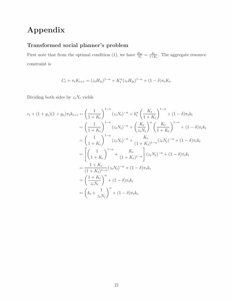
The relative price of investment sequence {πt} is pinned down as follows. We compute
the ratio of the purchasing power parity (PPP) price of investment to the PPP price of
consumption, both available from Penn World Table 7.1. From 1970 to 2007, we fit the data
with a second-degree polynomial and assign the fitted value to πt. After 2007, we assume
that πt remains constant at the 2007 fitted value. Figure 1 plots the relative price in the
data along with the fitted polynomial.
The population data are from the World Bank’s World Development Indicators. We set
gn to the observed average annual population growth for Korea from 1970 to 2007.
Next, we choose initial conditions for the model. We normalize the initial labor force
N0 = 1, leaving the initial capital per efficiency worker (k0) and the initial level of TFP
(z0) to be determined. We use two pieces of data for Korea in 1970 to help pin down these
two values. First, the share of the rural population is 60 percent. Second, we compute the
3Betts, Giri, and Verma (2011), Sposi (2012), Teignier (2012), and Uy, Yi, and Zhang (2013) are recentexamples of papers that study structural change in Korea. However, these papers do not consider the effectof changes in the relative price of investment. Furthermore, our focus is on the pace of industrialization in adual economy a la Lewis (1954), where the absorption of labor in the modern technology is affected by therate of capital formation.
10
capital stock in 1970 using investment series from Penn World Table 7.1 with the perpetual
inventory method and determine that the capital-output ratio in 1970 is 1.0. We then use
two equations from the model that determine the fraction of labor allocated to the traditional
technology and the capital-output ratio to match the two observed moments:
(1 + k0z0)−1
k0 · (k0 + 1/z0)−α
=
0.6
1.0
The solution to the above system is [k0, z0] = [1.58,0.42].
Finally, having chosen the parameter values and exogenous sequences, we choose the TFP
growth to match average annual per capita GDP growth in Korea from 1970 to 2007. Figure
2 plots the per capita GDP sequence from the model and the data.
Before we move to the counterfactual exercise, we discuss two implications of the model
that we do not target in the calibration. First, even though we calibrate only to the initial
share of rural population, the model is able to reproduce the observed decline in this share,
although the decline in the model is more rapid. In the data, the share of the rural population
declines to 42 percent in 1980 and 20 percent in 2005. In the model, the share declines to
42 percent in 1980 and 5 percent in 2005 as illustrated in Figure 3. Second, in the model,
investment as a share of GDP starts low and gradually increases to a constant level. This
feature of the investment rate is roughly consistent with the growth experience of Korea.
Over the 1970-2005 period, the investment rate increases from 20 percent to 35 percent in
the data. In the model, the investment rate starts at a lower level of 5 percent and increases
to 25 percent by 2005, an increase of 20 percentage points relative to the observed increase of
15 percentage points (Figure 4). Chang and Hornstein (2012), who focus on explaining the
dynamics of investment rates in Korea, also deliver the increasing pattern of investment rate
in a multisector model with declining capital goods prices. However, labor allocation across
sectors is exogenous in their model, so they do not address the issue of labor absorption
during the process of industrialization discussed in Lewis (1954) and Rostow (1956).
11
3.2 Counterfactuals
We now consider a counterfactual experiment in which Korea’s economy remains closed after
1969. Specifically, the closed economy is assumed to have a different sequence of the relative
price of investment but is otherwise identical to the benchmark open economy. That is, both
open and closed economies are subject to the same exogenous sequence of population and
TFP and have identical initial conditions.
To determine the counterfactual sequence of the relative price for the closed economy,
note that the price of investment relative to consumption in the data is fairly constant prior
to trade liberalization. The average annual change of the relative price in the data from 1953
to 1969 is close to zero. Consistent with this fact, we assume that in the closed economy the
relative price of investment is constant at the pre-liberalization (1969) level.
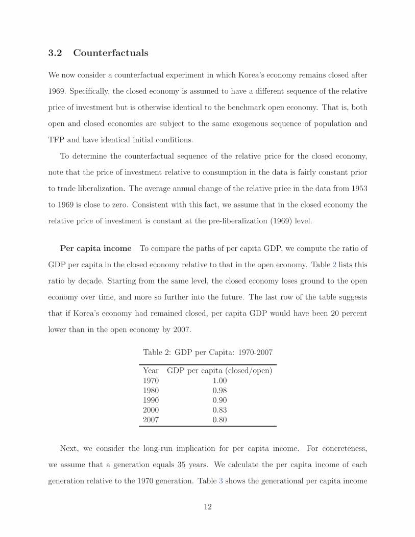
Per capita income To compare the paths of per capita GDP, we compute the ratio of
GDP per capita in the closed economy relative to that in the open economy. Table 2 lists this
ratio by decade. Starting from the same level, the closed economy loses ground to the open
economy over time, and more so further into the future. The last row of the table suggests
that if Korea’s economy had remained closed, per capita GDP would have been 20 percent
lower than in the open economy by 2007.
Table 2: GDP per Capita: 1970-2007
Year GDP per capita (closed/open)1970 1.001980 0.981990 0.902000 0.832007 0.80
Next, we consider the long-run implication for per capita income. For concreteness,
we assume that a generation equals 35 years. We calculate the per capita income of each
generation relative to the 1970 generation. Table 3 shows the generational per capita income
12
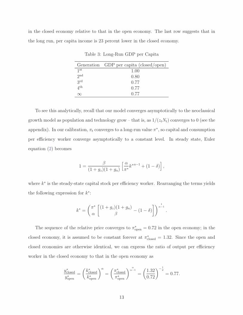
in the closed economy relative to that in the open economy. The last row suggests that in
the long run, per capita income is 23 percent lower in the closed economy.
Table 3: Long-Run GDP per Capita
Generation GDP per capita (closed/open)1st 1.002nd 0.803rd 0.774th 0.77∞ 0.77
To see this analytically, recall that our model converges asymptotically to the neoclassical
growth model as population and technology grow – that is, as 1/(ztNt) converges to 0 (see the
appendix). In our calibration, πt converges to a long-run value π∗, so capital and consumption
per efficiency worker converge asymptotically to a constant level. In steady state, Euler
equation (2) becomes
1 =β
(1 + gz)(1 + gn)
[ α
π∗k∗α−1 + (1− δ)
]
,
where k∗ is the steady-state capital stock per efficiency worker. Rearranging the terms yields
the following expression for k∗:
k∗ =
(
π∗
α
[
(1 + gz)(1 + gn)
β− (1− δ)
])1
α−1
.
The sequence of the relative price converges to π∗open = 0.72 in the open economy; in the
closed economy, it is assumed to be constant forever at π∗closed = 1.32. Since the open and
closed economies are otherwise identical, we can express the ratio of output per efficiency
worker in the closed economy to that in the open economy as
y∗closedy∗open
=
(
k∗closed
k∗open
)α
=
(
π∗closed
π∗open
)α
α−1
=
(
1.32
0.72
)− 1
2
= 0.77.
13
Thus, in the long run, the closed economy’s per capita income is 23 percent lower relative to
the open economy’s per capita income.
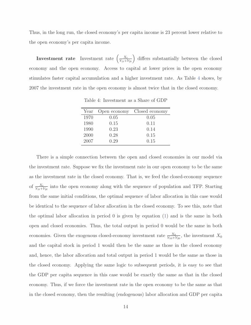
Investment rate Investment rate(
Xt
Y1t+Y2t
)
differs substantially between the closed
economy and the open economy. Access to capital at lower prices in the open economy
stimulates faster capital accumulation and a higher investment rate. As Table 4 shows, by
2007 the investment rate in the open economy is almost twice that in the closed economy.
Table 4: Investment as a Share of GDP
Year Open economy Closed economy1970 0.05 0.051980 0.15 0.111990 0.23 0.142000 0.28 0.152007 0.29 0.15
There is a simple connection between the open and closed economies in our model via
the investment rate. Suppose we fix the investment rate in our open economy to be the same
as the investment rate in the closed economy. That is, we feed the closed-economy sequence
of Xt
Y1t+Y2tinto the open economy along with the sequence of population and TFP. Starting
from the same initial conditions, the optimal sequence of labor allocation in this case would
be identical to the sequence of labor allocation in the closed economy. To see this, note that
the optimal labor allocation in period 0 is given by equation (1) and is the same in both
open and closed economies. Thus, the total output in period 0 would be the same in both
economies. Given the exogenous closed-economy investment rate X0
Y10+Y20, the investment X0
and the capital stock in period 1 would then be the same as those in the closed economy
and, hence, the labor allocation and total output in period 1 would be the same as those in
the closed economy. Applying the same logic to subsequent periods, it is easy to see that
the GDP per capita sequence in this case would be exactly the same as that in the closed
economy. Thus, if we force the investment rate in the open economy to be the same as that
in the closed economy, then the resulting (endogenous) labor allocation and GDP per capita
14
sequence are the same as those in the closed economy. (In this calculation, note that the
relative price of investment and the Euler equation (2) are irrelevant since we are directly
feeding in the investment rate.)
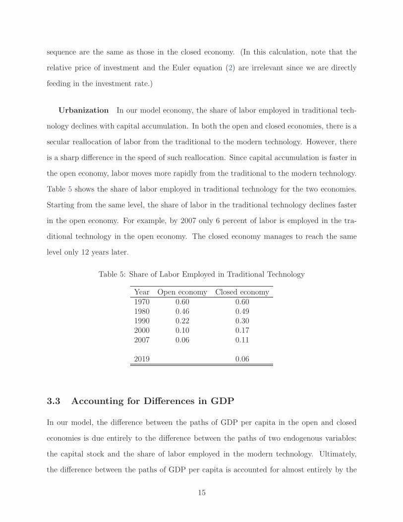
Urbanization In our model economy, the share of labor employed in traditional tech-
nology declines with capital accumulation. In both the open and closed economies, there is a
secular reallocation of labor from the traditional to the modern technology. However, there
is a sharp difference in the speed of such reallocation. Since capital accumulation is faster in
the open economy, labor moves more rapidly from the traditional to the modern technology.
Table 5 shows the share of labor employed in traditional technology for the two economies.
Starting from the same level, the share of labor in the traditional technology declines faster
in the open economy. For example, by 2007 only 6 percent of labor is employed in the tra-
ditional technology in the open economy. The closed economy manages to reach the same
level only 12 years later.
Table 5: Share of Labor Employed in Traditional Technology
Year Open economy Closed economy1970 0.60 0.601980 0.46 0.491990 0.22 0.302000 0.10 0.172007 0.06 0.11
2019 0.06
3.3 Accounting for Differences in GDP
In our model, the difference between the paths of GDP per capita in the open and closed
economies is due entirely to the difference between the paths of two endogenous variables:
the capital stock and the share of labor employed in the modern technology. Ultimately,
the difference between the paths of GDP per capita is accounted for almost entirely by the
15
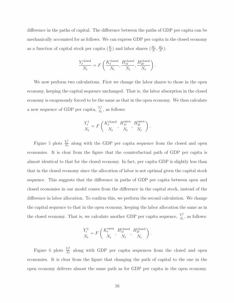
difference in the paths of capital. The difference between the paths of GDP per capita can be
mechanically accounted for as follows. We can express GDP per capita in the closed economy
as a function of capital stock per capita (KN) and labor shares (H1
N, H2
N):
Y closedt
Nt
= F
(
Kclosedt
Nt
,Hclosed
1t
Nt
,Hclosed
2t
Nt
)
.
We now perform two calculations. First we change the labor shares to those in the open
economy, keeping the capital sequence unchanged. That is, the labor absorption in the closed
economy is exogenously forced to be the same as that in the open economy. We then calculate
a new sequence of GDP per capita,Y 1t
Nt
, as follows:
Y 1t
Nt
= F
(
Kclosedt
Nt
,Hopen
1t
Nt
,Hopen
2t
Nt
)
.
Figure 5 plotsY 1t
Nt
along with the GDP per capita sequence from the closed and open
economies. It is clear from the figure that the counterfactual path of GDP per capita is
almost identical to that for the closed economy. In fact, per capita GDP is slightly less than
that in the closed economy since the allocation of labor is not optimal given the capital stock
sequence. This suggests that the difference in paths of GDP per capita between open and
closed economies in our model comes from the difference in the capital stock, instead of the
difference in labor allocation. To confirm this, we perform the second calculation. We change
the capital sequence to that in the open economy, keeping the labor allocation the same as in
the closed economy. That is, we calculate another GDP per capita sequence,Y 2t
Nt
, as follows:
Y 2t
Nt
= F
(
Kopent
Nt
,Hclosed
1t
Nt
,Hclosed
2t
Nt
)
.
Figure 6 plotsY 2t
Nt
along with GDP per capita sequences from the closed and open
economies. It is clear from the figure that changing the path of capital to the one in the
open economy delivers almost the same path as for GDP per capita in the open economy.
16
We conclude that the difference in GDP per capita between the closed and open economies is
driven entirely by faster capital accumulation in the open economy, which in turn is driven by
international access to cheaper capital goods. With less capital in the closed economy, labor
absorption per se does not yield more output since labor in the modern technology is not
as productive as in the open economy. Both mechanical accounts reinforce the argument in
Lewis (1954) and Rostow (1956) that the pace of industrialization and the speed of transition
to modern growth are limited by the amount of capital.
3.4 One-Sector Model
We have shown that access to capital at a lower price from the world market could signif-
icantly speed up capital formation, absorption of labor into the industrialized sector, and
the transition to modern growth. A natural question at this stage might be whether a one-
sector, open-economy model could deliver the rapid transition. By construction, the one-
sector model cannot be used to discuss the labor absorption into the industrialized sector
emphasized by Lewis (1954) and Rostow (1956). Nevertheless, the implications of declining
capital goods prices for other aspects of economic development can be investigated.
Suppose we consider an alternative version of the model in which the traditional technol-
ogy does not operate. That is, our benchmark model collapses into the neoclassical growth
model. To calibrate this model, let the sequences of the relative price of capital goods and
population remain the same as in the benchmark model. Choose the initial capital stock to
match the capital-output ratio in 1969. As before, normalize the initial TFP to be 1, and
choose the growth rate of TFP to match the average growth rate of per capita GDP between
1970 and 2007. The one-sector model predicts that the investment rate starts high and then
declines for several periods before it increases again. This U-shaped pattern of investment
rate is not consistent with the data. The fact that the standard neoclassical growth model is
at odds with the Korean data on investment rates was noted earlier by Chang and Hornstein
(2012). Our benchmark model, on the other hand, implies an increasing investment rate, a
17
pattern qualitatively consistent with the data. Furthermore, the pattern is consistent with
the observation in Lewis (1954) and Rostow (1956) that capital formation is slow at early
stages of development.
4 Conclusion
Capital formation has long been regarded as critical to the pace of industrialization and the
absorption of labor into the modern, industrialized sector. We argue that access to capital
goods in the world market at lower prices can speed up the process of industrialization. We
provide evidence from several countries that experienced major trade liberalizations in the
latter half of the twentieth century. In these countries, episodes of rapid growth coincide
with a continually declining relative price of investment after reform.
We construct a parsimonious open-economy growth model where both traditional and
modern technologies coexist similar to Lewis (1954). To test our theory, we first calibrate
the model to the postwar growth experience of Korea, taking the relative price of investment
as given from the data. We then perform a counterfactual experiment in which the relative
price of investment does not decline as observed in the data. We find that (i) the open-
economy investment rate is twice as high as the closed-economy investment rate in the long
run and (ii) the GDP per capita is 23 percent higher in the open economy. It also takes 12
more years for the closed economy to reduce the share of rural population to the same level
as the open economy. We also show through mechanical accounting exercises that the rate
of capital formation is the key driver of the differences between the paths of open and closed
economies.
18
References
Betts, C. M., R. Giri, and R. Verma (2011). Trade, Reform, and Structural Transformationin South Korea. Working Paper , University of Southern California.
Chang, Y. and A. Hornstein (2012). Transition Dynamics in the Neoclassical Growth Model:The Case of South Korea. Federal Reserve Bank of Richmond Working Paper No. 11-04R.
Connolly, M. and K.-M. Yi (2009). How Much of South Korea’s Growth Miracle Can BeExplained by Trade Policy? Federal Reserve Bank of Philadelphia Working Papers 09-19 .
Hansen, G. D. and E. C. Prescott (2002). Malthus to Solow. American Economic Re-
view 92 (4), 1205–17.
Heston, A., R. Summers, and B. Aten (July 2012). Penn World Table Version 7.1. Cen-ter for International Comparisons of Production, Income and Prices at the University ofPennsylvania.
Lewis, A. W. (1954). Economic Development with Unlimited Supplies of Labor. Manchester
School of Economic and Social Studies 22 (2), 139–91.
Nurkse, R. (1958). Problems of Capital Formation in Underdeveloped Countries. New York:Oxford University Press.
Parente, S. L. and E. C. Prescott (2002). Barriers to Riches. Cambridge, MA: MIT Press.
Ranis, G. and J. C. H. Fei (1961). A Theory of Economic Development. American Economic
Review 51 (4), 533–65.
Restuccia, D. and C. Urrutia (2001). Relative Prices and Investment Rates. Journal of
Monetary Economics 47 (1), 93–121.
Rodriguez, F. and D. Rodrik (2000). Trade Policy and Economic Growth: A Skeptic’sGuide to the Cross-National Evidence. In B. S. Bernanke and K. Rogoff (Eds.), NBERMacroeconomics Annual, Volume 15, pp. 261–338. Cambridge: MIT Press.
Rostow, W.W. (1956). The Take-Off into Self-Sustained Growth. Economic Journal 66 (261),25–48.
Rostow, W. W. (1960). The Stages of Economic Growth: A Non-Communist Manifesto.Cambridge, UK: Cambridge University Press.
Sposi, M. (2012). Evolving Comparative Advantage, Structural Change, and the Compositionof Trade. Working Paper , Federal Reserve Bank of Dallas.
Teignier, M. (2012). The Role of Trade in Structural Transformation. Working Paper ,Universitat de Barcelona.
Uy, T., K.-M. Yi, and J. Zhang (2013). Structural Change in an Open Economy. Journal ofMonetary Economics 60 (6), 667–82.
19
Westphal, L. E. (1990). Industrial Policy in an Export Propelled Economy: Lessons FromSouth Korea’s Experience. The Journal of Economic Perspectives 4 (3), 41–59.
20
Appendix
Transformed social planner’s problem
First note that from the optimal condition (1), we have H2t
Nt
= Kt
1+Kt
. The aggregate resource
constraint is
Ct + πtKt+1 = (ztH1t)1−α +Kα
t (ztH2t)1−α + (1− δ)πtKt.
Dividing both sides by ztNt yields
ct + (1 + gz)(1 + gn)πtkt+1 =
(
1
1 +Kt
)1−α
(ztNt)−α + kα
t
(
Kt
1 +Kt
)1−α
+ (1− δ)πtkt
=
(
1
1 +Kt
)1−α
(ztNt)−α +
(
Kt
ztNt
)α(Kt
1 +Kt
)1−α
+ (1− δ)πtkt
=
(
1
1 +Kt
)1−α
(ztNt)−α +
Kt
(1 +Kt)1−α(ztNt)
−α + (1− δ)πtkt
=
[
(
1
1 +Kt
)1−α
+Kt
(1 +Kt)1−α
]
(ztNt)−α + (1− δ)πtkt
=1 +Kt
(1 +Kt)1−α(ztNt)
−α + (1− δ)πtkt
=
(
1 +Kt
ztNt
)α
+ (1− δ)πtkt
=
(
kt +1
ztNt
)α
+ (1− δ)πtkt.
21
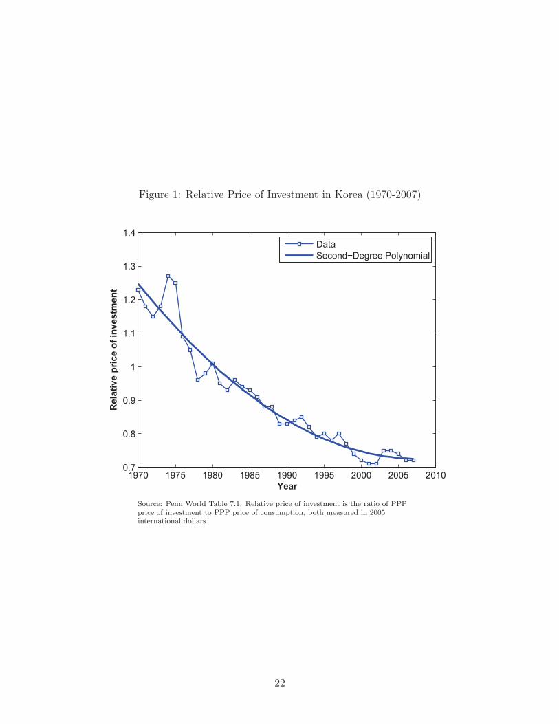
Figure 1: Relative Price of Investment in Korea (1970-2007)
1970 1975 1980 1985 1990 1995 2000 2005 20100.7
0.8
0.9
1
1.1
1.2
1.3
1.4
Year
Rela
tive p
rice o
f in
vestm
en
t
Data
Second−Degree Polynomial
Source: Penn World Table 7.1. Relative price of investment is the ratio of PPPprice of investment to PPP price of consumption, both measured in 2005international dollars.
22
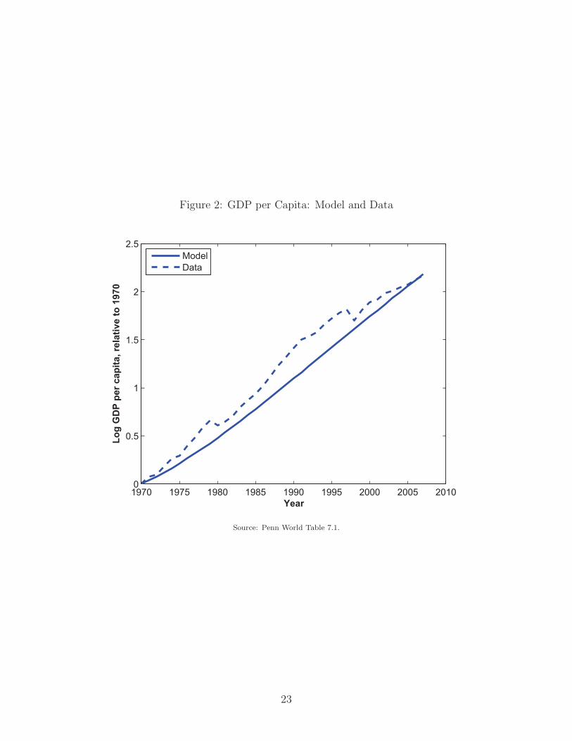
Figure 2: GDP per Capita: Model and Data
1970 1975 1980 1985 1990 1995 2000 2005 20100
0.5
1
1.5
2
2.5
Year
Lo
g G
DP
per
cap
ita,
rela
tive t
o 1
970
Model
Data
Source: Penn World Table 7.1.
23
Figure 3: Share of Rural Population: Model and Data
1970 1975 1980 1985 1990 1995 2000 2005 20100
0.1
0.2
0.3
0.4
0.5
0.6
0.7
Year
Sh
are
of
rura
l p
op
ula
tio
n
Model
Data
Source: World Development Indicators.
24
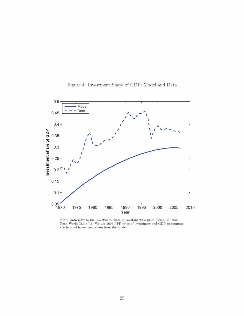
Figure 4: Investment Share of GDP: Model and Data
1970 1975 1980 1985 1990 1995 2000 2005 20100.05
0.1
0.15
0.2
0.25
0.3
0.35
0.4
0.45
0.5
Year
Investm
en
t sh
are
of
GD
P
Model
Data
Note: Data refer to the investment share in constant 2005 price (series ki) fromPenn World Table 7.1. We use 2005 PPP price of investment and GDP to computethe implied investment share from the model.
25
Figure 5: GDP per Capita: Closed-Economy Capital and Open-Economy Labor
1970 1975 1980 1985 1990 1995 2000 2005 20100
0.5
1
1.5
2
2.5
Year
Lo
g G
DP
per
cap
ita
Benchmark: Open−Economy Capital, Open−Economy Labor
Closed−Economy Capital, Closed−Economy Labor
Closed−Economy Capital, Open−Economy Labor
26
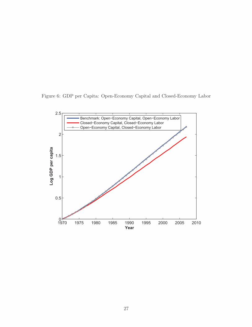
Figure 6: GDP per Capita: Open-Economy Capital and Closed-Economy Labor
1970 1975 1980 1985 1990 1995 2000 2005 20100
0.5
1
1.5
2
2.5
Year
Lo
g G
DP
per
cap
ita
Benchmark: Open−Economy Capital, Open−Economy Labor
Closed−Economy Capital, Closed−Economy Labor
Open−Economy Capital, Closed−Economy Labor
27