The Propagation of Monetary Policy Shocksin a Heterogeneous Production Economy∗

Ernesto Pasten†, Raphael Schoenle‡, and Michael Weber§

December 2019

Abstract

Realistic heterogeneity in price rigidity interacts with heterogeneity in sectoralsize and input-output linkages in the transmission of monetary policy shocks.Quantitatively, heterogeneity in price stickiness is the central driver for real effects.Input-output linkages and consumption shares alter the identity of the mostimportant sectors to the transmission. Reducing the number of sectors decreasesmonetary non-neutrality with a similar impact response of inflation. Hence, theinitial response of inflation to monetary shocks is not sufficient to discriminate acrossmodels and ignoring heterogeneous consumption shares and input-output linkagesidentifies the wrong sectors from which the real effects originate.

JEL classification: E30, E32, E52

Keywords: Input-output linkages, multi-sector Calvo model, monetary policy

∗We thank Klaus Adam, Susanto Basu, Carlos Carvalho, Zeno Enders, Xavier Gabaix, Gita Gopinath,Yuriy Gorodnichenko, Bernard Herskovic, Hugo Hopenhayn, Pete Klenow, Alireza Tahbaz-Salehi, HaraldUhlig, and conference and seminar participants at the Annual Inflation Targeting Seminar of the BancoCentral do Brasil, AEA, Banque de France Conference on Price Setting and Inflation, BIS, Brandeis,Cambridge, Carlos III, Cleveland Fed conference on Inflation: Drivers and Dynamics Conference, EEA,Einaudi, FGV Sao Paulo, Konstanz seminar on Monetary Theory, Oxford, St. Louis Fed, SED, Toulouse.Pasten is grateful for the support of the Universite de Toulouse Capitole during his stays in Toulouse.Weber thanks the Fama-Miller Center at the University of Chicago Booth School of Business and theFama Research Fund for financial support. Schoenle and Weber also acknowledge financial support fromthe National Science Foundation under grant 1756997. We also thank Will Cassidy, Seongeun Kim, MattKlepacz and Michael Munsell for excellent research assistance. Any views expressed are only those of theauthors and do not necessarily represent the views of the ECB or the Eurosystem, the Cleveland FEDor the Federal Board System, or the Central Bank of Chile.†Central Bank of Chile and Toulouse School of Economics. e-Mail: ernesto.pasten@tse-fr.eu‡Cleveland Fed, CEPR, and Brandeis University. e-Mail: schoenle@brandeis.edu.§University of Chicago Booth School of Business and NBER. e-Mail:

michael.weber@chicagobooth.edu.

I Introduction

Understanding how monetary policy transmits to the real economy and why nominalshocks have real effects are vital questions in monetary economics. The literatureidentified heterogeneity in price rigidities as a central driver behind the real effects ofmonetary shocks (see, e.g., Carvalho (2006) and Nakamura and Steinsson (2008)) buta recent literature suggests other heterogeneities on the production side might also beimportant for aggregate fluctuations. Sectors differ in size and different sectors usedifferent intermediate input mixes to produce output. Gabaix (2011) and Acemoglu,Carvalho, Ozdaglar, and Tahbaz-Salehi (2012) derive conditions under which theseheterogeneties can generate aggregate fluctuations from idiosyncratic or sectoral realshocks invalidating the diversification argument of Lucas (1977) and Ozdagli and Weber(2017) argue production networks shape the stock market response to monetary shocks.But most of the existing literature has studied how heterogeneities in sector size,input-output structure, and price stickiness shape aggregate fluctuations in isolation.

The analysis in this paper presents new theoretical insights into the transmission ofmonetary policy shocks in an economy in which all three heterogeneities are present andinteract with each other. First, we show real effects of nominal shocks are bigger if theshare of intermediate inputs is high or if sticky-price sectors are important suppliers tothe rest of the economy, to large sectors and to flexible-price sectors on impact, but tosticky price sectors following the shock.1 Second, the level of disaggregation is central forthe real effects of monetary policy. More granular economies result in larger real effectswith similar price responses on impact. Third, the importance of specific sectors for thetransmission of monetary policy shocks depends on which heterogeneities are present, andhow they interact.

On the quantitative side, our contribution lies in the calibration of a detailed modelof the U.S. economy to study the quantitative importance of the different types ofheterogeneities. We calibrate a 341-sector version of the model to the input-output (I/O)tables from the Bureau of Economic Analysis (BEA) and the micro-data underlying theproducer price index (PPI) from the Bureau of Labor Statistics (BLS). First, heterogeneityin price stickiness is the main driver of real output effects: It increases real output effectsrelative to an economy with homogeneous price stickiness by 70%. Additionally allowingfor heterogeneity in consumption shares or size or both only has a marginal effect onimpact and on cumulative real output effects.

Second, the choice of disaggregation plays an important role quantitatively. A 341-sector economy has a 6% (49%) larger cumulative real effect of monetary policy shocksthan a less granular 58-(7-)sector model. However, across choices of aggregation, theresponse of inflation to the monetary policy shock is similar on impact and on averageduring the first few periods. The large differences in real output effects with similarimpact responses of inflation across different levels of aggregation caution against drawinginference for the conduct of monetary policy from the initial response of inflation tomonetary policy shocks.

1Some of the results are well known. The dynamic prediction in the network setting is most distinctlynew (see Basu (1995), Huang and Liu (2001, 2004), Shamloo (2010)), and Bouakez, Cardia, and Ruge-Murcia (2014))

2

Third, heterogeneity in price rigidity is key in determining which sectors are themost important contributors to the transmission of monetary shocks. In an economywith homogeneous price stickiness all sectors respond equally to a common monetarypolicy shock independent of their size or I/O structure. Once we introduce differentprice stickiness across sectors, sectoral output responses of the 10 most important sectorsincrease by 350%. Hence, heterogeneous price stickiness is central for differential sectoralreal effects, but this result does not mean that heterogeneities in sector size and I/Ostructure does not matter for sectoral responses. Our baseline economy with all threeheterogeneities present doubles the real effects of the ten most important sectors relativeto the economy with homogeneous sector size and I/O structure and totally scramblesthe identities of the 10 most important, contractionary responses. Thus, even thoughheterogeneity in I/O linkages or size only has a marginal effect on the aggregate realoutput responses, which sector transmits the monetary policy shock the most dependscrucially on the exact specification of heterogeneities. As we remove heterogeneities, thedistribution of responses also becomes much more compressed.

Notably, heterogeneity in price rigidity also changes the sign of the response for theleast contractionary responses: In fact, the 10 least contractionary sectoral responses arepositive in all combinations that include heterogeneity in price rigidity. As we removeheterogeneities from the baseline, responses also become more compressed and smaller –but only negative when price rigidity becomes homogeneous. The flip in sign is due tothe fact that the 10 least contractionary, expansionary responses are concentrated in themost flexible sectors. These sectors can gain market share from lowering their relativeprices more quickly than stickier-price sectors.

Taken together, these results show (i) Heterogeneous price stickiness is the centralforce for the real effects of nominal shocks; heterogeneity in intermediate input usage andin the I/O structure is less important; (ii) disaggregation matters for the real effects ofmonetary policy shocks but leaves the impact response of inflation largely unchanged;(iii) price stickiness that differs across sectors changes the identity and importance of themost important sectors for the transmission of monetary shocks; (iv) heterogeneous sectorsize and I/O structures further change the identity of the most important sectors for thereal effects of monetary shocks and increase their importance, and hence, the effectivegranularity of the economy increases.

What mechanisms drive these results? In the model, firms set prices as a markup overa weighted average of future marginal costs. Our analysis identifies four distinct channelsthrough which I/O linkages and the heterogeneities of sector size and price stickinessaffect the marginal-cost process. First, marginal costs of final-goods producers dependdirectly on the sector-specific input price index. Second, sector-specific wages dependindirectly on I/O linkages because the optimal mix of inputs depends on the relative priceof intermediate inputs and labor. Third and fourth, the heterogeneities across sectors intotal production, value-added, and intermediate inputs create wedges between sectoralparticipation in total output, production, and total GDP that feed back into marginalcosts. These channels interact in shaping the response to nominal shocks in a very intuitiveway: How important is the output of a given sector for final-goods production? Howflexible are the output prices of the goods the sector uses in production? How importantis the sector as a producer for total consumption?

3

We develop further, analytical intuition for the interaction of the three heterogeneitiesin a simplified model. In this economy, we gradually add each heterogeneity, and proveresults analytically when possible. We start with an economy that features I/O linkagesthat can be homogeneous or heterogeneous across sectors. Key to this step is that pricerigidity is homogeneous across sectors, and sectoral participation in GDP equals sectoralparticipation in total production. I/O linkages per se amplify the real effects of monetarypolicy, as in Nakamura and Steinsson (2008). However, heterogeneity in consumptionshares and I/O linkages does not matter, because sectoral production and consumptionshares do not produce wedges.

We then add heterogeneity in Calvo parameters. This addition generates a hump-shaped response in consumption, because flexible-price firms compete with sticky-pricefirms. Firms with flexible prices adjust prices in a staggered fashion and by less on impactthan in a model with homogeneous Calvo rates across sectors. The dispersion of pricestickiness amplifies cumulative real effects following an identical impact of consumptionas in Carvalho (2006), Carvalho and Schwartzman (2015), and Alvarez et al. (2016).Heterogeneity in I/O linkages and consumption shares does not affect the impact responserelative to an economy with homogeneous price stickiness and also does not have anysystematic effect following the impact response.

Last, we allow for fully unrestricted heterogeneity in sector weights in GDP and in I/Olinkages. This additional degree of heterogeneity results in wedges between consumptionprices and sectoral intermediate input prices, which influence sectoral marginal costs.Heterogeneity in I/O linkages can amplify or dampen the output response. For example,the economy may resemble more of a flexible-price economy or a sticky-price economy,depending on the interaction of sector size, the importance of sectors as suppliers toother sectors, and sectoral price stickiness. We characterize the interactions and theirinfluence on real effects of monetary policy by three relations: (i) first-order out-degreesto sector size, (ii) first-order outdegrees adjusted by average flexibility to sector size, and(iii) covariances between sectoral linkages and size with price stickiness.

A. Literature Review

Our paper contributes new insights to the literature on the transmission of monetarypolicy shocks in a network economy. Basu (1995) shows a roundabout productionstructure can magnify the importance of price rigidities through its effect on marginalcosts, and results in larger welfare losses of demand-driven business cycles. Huangand Liu (2001, 2004) study the persistence of monetary shocks in a multi-sector modelwith roundabout production and fixed contract length. Aggregate output becomesmore persistent in the their setup the higher the number of production stages andthe share of intermediates. Their work theoretically shows that intermediate inputsamplify the importance of rigid prices with no impact on wage stickiness. Nakamuraand Steinsson (2010) develop a multi-sector menu-cost model and show in a calibration ofa six-sector version that heterogeneity in price stickiness together with I/O linkages canexplain persistent real effects of nominal shocks with moderate degrees of price stickiness.Carvalho and Lee (2011) show a multi-sector Calvo model with intermediate inputs canreconcile why firms adjust more quickly to idiosyncratic shocks than to aggregate shocks

4

(see also Boivin et al. (2009) and Shamloo (2010)). Bouakez, Cardia, and Ruge-Murcia(2014) estimate a multi-sector Calvo model with production networks using aggregateand sectoral data, and find evidence of heterogeneity in frequencies of price adjustmentsacross sectors.

We contribute several new insights to this literature. Our most importantquantitative innovation is to study the importance of networks on the propagation ofnominal shocks in a detailed, 341-sector calibration of the U.S. economy. Second, we showboth theoretically and quantitatively that reducing the number of sectors in the modeldecreases monetary non-neutrality. By contrast, across calibrations the impact responseof inflation is similar across aggregation choices, and hence is not a sufficient statistic formonetary non-neutrality. Finally, we point out a new identity effect: Heterogeneity inprice rigidity is key in determining which sectors are the most important contributors tothe transmission of monetary shocks but heterogeneity in sector size and I/O structure canchange the sectoral identify substantially, and makes important contributors even moreimportant and down-weighs the contribution of less important sectors. A few sectors withflexible prices can also increase their output following a contractionary shock, given theirfall in relative price.

A high degree of specialization is a general, key feature of modern productioneconomies. Gabaix (2011) and Acemoglu et al. (2012) show theoretically the networkstructure and the firm-size distribution are potentially important propagation mechanismsfor aggregate fluctuations originating from firm and industry shocks. Acemoglu, Akcigit,and Kerr (2015) and Barrot and Sauvagnat (2016) show empirical evidence for thepropagation of idiosyncratic supply shocks through the I/O structure. Carvalho (2014)provides an overview of this fast-growing literature. Idiosyncratic shocks propagatethrough changes in prices. In companion papers (see Pasten, Schoenle, and Weber (2018)and Cox, Mueller, Pasten, Schoenle, and Weber (2019)), we study how price rigiditiesaffect the importance of idiosyncratic shocks as an origin of aggregate fluctuations andthe size of fiscal multipliers.

Other recent applications of production networks in different areas of macroeconomicsinclude Bigio and La’O (2017) who study the amplification of financial frictions throughproduction networks, and Ozdagli and Weber (2017), who empirically show I/O linkagesare a key propagation channel of monetary policy to the stock market. Additionally,Kelly, Lustig, and Van Nieuwerburgh (2013) study the joined dynamics of the firm-sizedistribution and stock return volatilities. Herskovic, Kelly, Lustig, and Van Nieuwerburgh(2016) and Herskovic (2018) study asset-pricing implications of production networks.

II Model

This section presents the full blown New Keynesian model. We highlight in particularhow heterogeneities in price rigidities, sectoral size, and I/O linkages enter the model.

5

A. Firms

A continuum of monopolistically competitive firms j operates in different sectors. Weindex firms by their sector, k = 1, ..., K, and by j ∈ [0, 1]. The set of consumptiongoods is partitioned into a sequence of subsets =kKk=1 with measure nkKk=1 such that∑K

k=1 nk = 1.The first, real heterogeneity – heterogeneity in sectoral I/O linkages – enters via the

production function of firm j in sector k

Ykjt = L1−δkjt Z

δkjt, (1)

where Lkjt is labor and Zkjt is an aggregator of intermediate inputs

Zkjt ≡

[K∑r=1

ω1η

krZkjt (r)1− 1η

] ηη−1

. (2)

Here, Zkjt (r) denotes the intermediate input use by firm j in sector k in period t. The

aggregator weights ωkrk,r satisfy∑K

r=1 ωkr = 1 for all sectors k. We allow these weightsto differ across sectors, which is a central ingredient of our analysis.

In turn, Zkjt (r) is an aggregator of goods produced in sector r,

Zkjt (r) ≡[n−1/θr

∫=rZkjt (r, j′)

1− 1θ dj′

] θθ−1

. (3)

Zkjt (r, j′) is the amount of goods firm j′ in sector r produces that firm k, j uses as input.Demand for intermediate inputs Zkjt (r) and Zkjt (r, j′) is given by the following

demand equations

Zkjt (r) = ωkr

(PrtPkt

)−ηZkjt,

Zkjt (r, j′) =1

nr

(Prj′tPrt

)−θZkjt (r) .

Prj′t is the price firm j′ in sector r charges, Prt is a sectoral price index, and Pkt isan input-price index; we define both price indices below. In steady state, all prices areidentical, and ωkrKr=1 is the share of costs that firm k, j spends on inputs from sector r

and, hence, equals cell k, r in the I/O Tables (see online appendix). We refer to ωkrKr=1

as “I/O linkages.” As a result, in steady state, all nr firms in sector r share the demandof firm k, j for goods that sector r produces equally.

Away from steady state, a gap exists between the price index of sector r, Prt, andthe input price index, Pkt, that is relevant for firms in sector k. It distorts the share ofsector r in the costs of firms in sector k. Similarly, price dispersion across firms withinsector r determines the dispersion of demand of firms in sector k for goods in sector r.

6

Price indices relevant for the demand of intermediate inputs across sectors are defined as

Pkt =

[K∑r=1

ωkrP1−ηrt

] 11−η

,

Prt =

[1

nr

∫=rP 1−θrj′t dj

′] 1

1−θ

.

Our second heterogeneity – heterogeneity of price rigidity – originates from the assumptionabout price setting. Firms set prices as in Calvo (1983), but we allow for differences inCalvo rates across sectors, αkKk=1. That is, the objective of firm j, k is given

maxPkjt

Et∞∑s=0

Qt,t+sαsk [PkjtYkjt+s −MCkt+sYkjt+s] , (4)

where MCkt = 11−δ

(δ

1−δ

)−δW 1−δkt (Pkt)

δ are marginal costs after imposing the optimalmix of labor and intermediate inputs

δWktLkjt = (1− δ)PktZkjt. (5)

The optimal pricing problem takes the standard form

∞∑s=0

Qt,t+sαskYkjt+s

[P ∗kt −

θ

θ − 1MCkjt+s

]= 0. (6)

Ykjt+s is the total output of firm k, j at period t+s, Qt,t+s is the stochastic discount factorbetween period t and t+ s, and θ is the elasticity of substitution within sector.

The optimal price for all adjusting firms within a given sector is identical, P ∗kt, allowingsimple aggregation. Hence, the law of motion for sectoral prices is

Pkt =[(1− αk)P ∗1−θkt + αkP

1−θkt−1

] 11−θ ∀k. (7)

B. Households

A large number of infinitely lived households exist. Households have a love for variety,and derive utility from consumption and leisure. Households supply all different types oflabor. The representative household has additively separable utility in consumption andleisure and maximizes

maxE0

∞∑t=0

βt

(C1−σt − 1

1− σ−

K∑k=1

∫=kgkL1+ϕkjt

1 + ϕdj

)(8)

7

subject to

PCtCt =K∑k=1

Wkt

∫=kLkjtdj +

K∑k=1

Πkt + It−1Bt−1 −Bt. (9)

The budget constraint states nominal expenditure equals nominal household income. Ctand PCt are aggregate consumption and prices, which we define below. Lkjt and Wkt

are labor employed and wages paid by firm j in sector k. Households own firms andreceive net income, Πkt, as dividends. Bonds, Bt, pay a nominal gross interest rate ofIt−1. gkKk=1 are parameters that we choose to ensure a symmetric steady state acrossall firms.

Aggregate consumption is

Ct ≡

[K∑k=1

ω1η

ckC1− 1

η

kt

] ηη−1

, (10)

where Ckt is the aggregation of sectoral consumption

Ckt ≡[n−1/θk

∫=kC

1− 1θ

kjt dj

] θθ−1

. (11)

Ckjt is the consumption of goods that firm j in sector k produces.We allow the elasticity of substitution across sectors η to differ from the elasticity

of substitution within sectors θ. Consumption weights ωck can also differ acrosssectors, which is the third heterogeneity across sectors in the model. The weights satisfy∑K

k=1 ωck = 1.Households’ demand for sectoral goods Ckt and firm goods Ckjt is

Ckt = ωck

(PktPCt

)−ηCt,

Ckjt =1

nk

(PkjtPkt

)−θCkt.

We solve in the online appendix for the steady state of the economy. We showthe consumption weights ωckKr=1 determine the steady-state shares of sectors in total

consumption (or value-added production). In the following, we refer to ωckKr=1 as“consumption shares.” Heterogeneity in sectoral size enters through these shares. Awayfrom steady state, a gap between sectoral prices, PrtKr=1, and aggregate consumptionprices, PCt, distorts the share of sectors in aggregate consumption.2

2The measure of firms in sector k, nk, and the consumption shares are related in equilibrium (seeonline appendix).

8

The consumption price index PCt is given by

PCt =

[K∑k=1

ωckP1−ηkt

] 11−η

, (12)

and sectoral prices follow

Pkt =

[1

nk

∫=kP 1−θkjt dj

] 11−θ

. (13)

C. Monetary policy

The monetary authority sets the short-term nominal interest rate, It, according to aTaylor rule

It =1

β

(PCtPCt−1

)φπ (CtC

)φyeµt . (14)

µt is a monetary shock following an AR(1) process with persistence ρµ. Thus, monetarypolicy reacts to aggregate consumption inflation and aggregate consumption.

In quantitative exercises of the analysis, we also study economies with interest ratessmoothing similar to Coibion and Gorodnichenko (2012).

D. Equilibrium conditions and definitions

Bt = 0, (15)

Lkt =

∫=kLkjtdj, (16)

Wt ≡K∑k=1

nkWkt, (17)

Lt ≡K∑k=1

Lkt, (18)

Ykjt = Ckjt +K∑k′=1

∫=k′

Zk′j′t (k, j) dj′. (19)

Equation (15) is the market-clearing condition in bond markets. Equation (16)defines aggregate labor in sector k. Equations (17) and (18) give aggregate wage (which isa weighted average of sectoral wages) and aggregate labor (which linearly sums up hoursworked in all sectors). Equation (19) is Walras’ law for the output of firm j in sector k.

9

III Heterogeneities and Marginal Costs

The dynamic behavior of marginal costs is crucial for understanding the response of theeconomy to a monetary policy shock. This section develops intuition for the effects ofheterogeneity in price stickiness, I/O linkages, and sectoral size on marginal costs, andthe real effects of monetary policy in a log-linearized system that we detail in the onlineappendix. In the following, small letters denote log deviations from steady state. Wefocus on the role of heterogeneity in I/O linkages. Our main, analytical propositions inthe next section, however, do not require reading this section first.

We highlight how I/O linkages affect marginal costs and demand through four distinctchannels. In particular, a new wedge emerges that drives marginal costs: I/O linkagescreate a difference between the aggregate consumption price index and intermediate inputprice indices that affects marginal costs.

The reduced-form system that embeds marginal costs has K + 1 equations andunknowns: value-added production ct and K sectoral prices pktk=1. The first equationis

σEt [ct+1]− (σ + φc) ct + Et [pct+1]− (1 + φπ) pct + φπpct−1 = µt, (20)

which is a combination of the household Euler equation and the Taylor rule. The equationdescribes how variations in value-added production, ct, and aggregate consumption prices,pct, respond to the monetary policy shock, µt.

Note pct is given by

pct =K∑k=1

ωckpkt. (21)

In addition, K equations governing sectoral prices

βEt [pkt+1]− (1 + β) pkt + pkt−1 = κk (pkt −mckt) , (22)

complete the system, where κk ≡ (1− αk) (1− αkβ) /αk measures the degree of priceflexibility.

A. The effect of I/O linkages on marginal cost

Here, we show that I/O linkages crucially affect marginal costs. We distinguish betweenthe use of intermediate inputs per se (i.e., δ > 0) and heterogeneous usage of intermediateinputs across sectors (i.e., ωkr 6= ωk′r ∀k,∀k′ 6= k, and ∀r). Although our focus is on I/Olinkages, heterogeneity in sectoral size ωck and in pricing frictions is also present throughκk. We first derive how I/O linkages affect several intermediate, key variables.

First, I/O linkages affect the measure of sectors, nkKk=1. The measure reflects theweighted average of the consumption share of sector k, ωck, and the importance of sectork as a supplier to the economy, ζk

nk = (1− ψ)ωck + ψζk, (23)

10

where

ζk ≡K∑k′=1

nk′tωk′k. (24)

We refer to ζk as the “outdegree” of sector k, analogous to Acemoglu et al. (2012). Theoutdegree of sector k is the weighted sum of intermediate input use from sector k by allother sectors ωk′k, with weights nk′t. In steady state, all firms are identical and we caninterpret nk as the size of sector k.

Without intermediate inputs (δ = 0), ψ ≡ δ (θ − 1) /θ = 0, and only consumptionshares determine sector size. By contrast, when firms use intermediate inputs forproduction (δ > 0), heterogeneity in I/O linkages results in additional heterogeneitiesin sector size. The outdegree of sector k is higher when sector k is a supplier to manysectors or is a supplier of large sectors.

The vector ℵ of sector sizes nkKk=1 solves

ℵ = (1− ψ) [IK − ψΩ′]−1

ΩC , (25)

where IK is the identity matrix of dimension K, Ω is the I/O matrix in steady state withelements ωkk′, and ΩC is the vector of consumption shares, ωck.

Second, heterogeneity in I/O linkages implies each sector faces a different intermediateinput price index

Pkt =K∑k′=1

ωkk′Pk′t. (26)

In particular, the sector-k intermediate input price index responds more to variation inthe prices of another sector k′ when that sector is a large supplier to sector k.

A.1 Direct effect on sectoral marginal costs

With intermediate inputs in production (δ > 0), sectoral marginal costs are a weightedaverage of sectoral wages, but also sectoral intermediate input price indices

mckt = (1− δ)wkt + δpkt. (27)

The sectoral intermediate input price index, Pkt, reflects heterogeneity in I/O linkages.All else equal, an increase in the price of another sector k′ implies higher costs of theintermediate inputs. Heterogeneity in I/O linkages allows this channel to differ acrosssectors.

A.2 Indirect effect through sectoral wages

I/O linkages also affect sectoral wages wkt indirectly because the efficient mix of laborand intermediate inputs in equation (5) depends on relative input prices. The production

11

function implicitly defines sectoral labor demand for a given level of production ykt

ykt = lkt + δ (wkt −Pkt) . (28)

In a model without I/O linkages (δ = 0), sectoral labor demand is inelastic afterconditioning on sectoral production ykt. Here, I/O linkages (δ > 0) imply labor demanddepends negatively on wages, because higher wages lead firms to substitute labor forintermediate inputs.

Combining the production function and sectoral labor supply yields

wkt =1

1 + δϕ[ϕykt + σct + δϕ (Pkt − pct)] + pct. (29)

Thus, the optimal choice implies a wedge between sectoral intermediate input prices andaggregate consumption prices, (Pkt − pct).

What is the role of this wedge? In a model without I/O linkages (δ = 0), wagesrespond one to one to variations in aggregate consumption prices pct through their effecton labor supply. An increase in sector k′ prices positively affects wages in sector k. Therelevant elasticity is tied to the consumption share of sector k′, ωck′ . This effect is capturedby the last term of equation (29).

In the presence of I/O linkages (δ > 0), this last term continues to affect wages.However, the wedge (Pkt − pct) now additionally comes into play: An increase in sectork′ prices has an additional, positive effect on sector k wages when the share of sector k′

as a supplier of sector k is larger than its consumption share, that is, when ωkk′ > ωck′ .Intuitively, if sector k′ is a large supplier to sector k, a positive variation in pk′t has alarger effect on increasing the cost of intermediate inputs for firms in sector k. As a result,firms in sector k increase the demand for labor, and sector k wages go up.

A.3 Effect on sectoral demand

Next, we show I/O linkages can heterogeneously affect the response of sectoral demand,yktKk=1. This follows because sectoral demand is given by

ykt =(1− ψ)ωck

nkckt +

ψ

nk

K∑k′=1

nk′ωk′kzk′t (k) for all k, (30)

where nk is size of sector k as defined in (23), and ckt and zk′t (k) repectively are log-lineardeviations of sector k’s demand for consumption and intermediate inputs from firms insector k′. In turn, the log linear versions of these demands are

ckt = ct − η (pkt − pct) ,zk′t (k) = zk′t − η (pkt −Pk′t) .

12

so sectoral demand yk is given by

ykt =

[(1− ψ)ωck

nkct +

ψ

nk

K∑k′=1

nk′ωk′kzk′t

]+

η

[pkt −

(1− ψ)ωcknk

pct +ψ

nk

K∑k′=1

nk′ωk′kPk′t

]

Taking as given real aggregate demand from households ct and from firms in allsectors zk′tKk′=1, real demand from sector k depends on the extent that monetary policydifferently affect its own prices pkt and the weighted average of aggregate consumptionprices pct and all sector-specific aggregate intermediate inputs prices Pk′tKk′=1. Theresponsivenes of these sector-specific aggregate prices depends the whole input-outputstructure of the economy in steady state.

A.4 Effect on aggregate demand

Finally, the way that aggregate demand of intermediate inputs zt responds to monetaryshocks also depends on the heterogeneity in I/O linkages. We solve for zt, combiningWalras’ law, the aggregate production function, aggregate labor supply, and theaggregation of efficient mixes between labor and intermediate inputs,

zt =[(1 + ϕ) (1− ψ) + σ (1− δ)] ct − (1− δ) (pt − pct)

(1− ψ) + ϕ (δ − ψ). (31)

where pct is, as through the whole paper, the consumption aggregate price and pt is thewhole-economy intermediate inputs aggregate price, pt =

∑k ζkpkt.

In an economy with no I/O linkages (δ = 0, ψ = 0), output equals consumption,yt = ct. With intermediate inputs (δ > 0), zt varies positively with ct: More value-addedproduction requires more intermediate inputs. This channel shows up as the first termin the numerator of equation (31). At the same time, an increase in prices of a givensector k′ has negative effect on zt when that sector is central in the economy. This secondeffect is captured by the wedge (pt − pct), the second term in the numerator of equation(31), equivalent to the condition that sectors are relatively more central than their GDPshare implies: ζk′ > ωck′ . Then, an increase in prices of big suppliers in the economyresults in higher prices for intermediate inputs for many sectors and/ or bigger sectors.These sectors then substitute intermediate inputs for labor, and the aggregate demandfor intermediate inputs decreases.

B. Overall solution for log-linearized marginal costs

All these indirect effects altogether imply that sectoral wages have heterogeneous effectson the determination of other sectoral wages through input-output linkages,

wt = Φ−1 [Γcct + Γppt] (32)

13

such that

Φ = (1 + δϕ) IK − (1 + ϕ)ψN−1ΩN;

Γc =[σIK − ψN−1Ω′N

]ι+ ϕ (1− ψ)N−1ΩC ;

Γp =[IK − ψN−1Ω′N

]ιΩC′ − ϕη

[IK − (1− ψ)NΩCΩC′]

+ϕ[(η − 1)ψN−1Ω′N− δIK

]Ω.

where wt and pt respectively are the vector of sectoral wages, N is a diagonal matrix withthe vector of sectoral size in its diagonal, IK is the identity matrix of dimension K, Ω isthe I/O matrix in steady state with elements ωkk′, and ΩC is the vector of consumptionshares, ωck.

To get the final expression for the vector of sectoral marginal costs, mct, the solutionfor sectoral wages must be plugged into

mct = (1− δ)wt + δΩpt (33)

By contrast, in an otherwise identical economy with no I/O linkages (δ = 0), marginalcosts are given by

mcδ=0kt = (1 + ϕη) pct − ϕηpkt + (σ + ϕ) ct. (34)

There, an increase in prices of other sectors, pk′t, increases marginal costs. Thiseffect uniformly depends on elasticities 1 + ϕη, and specifically, on the heterogeneityin consumption shares ωck′ .

IV Theoretical Results

Here, we present new, closed-form results for the response of inflation and consumption toa monetary policy shock. In doing so, we benchmark our economy with heterogeneity inprice rigidity against an economy in which prices are homogeneously rigid. We highlighthow the I/O structure interacts with the pricing frictions and heterogeneity in sectoral sizeand shapes our results. The identity effect – which sector contributes the most to monetarytransmission – can be crucially affected by the interaction of heterogeneities. Also, thelevel of aggregation can be key for the degree of monetary non-neutrality. The latter twoinsights provide important guidance for monetary policymakers trying to correctly assessthe most important sectors for the transmission of monetary policy shocks to output andinflation.

A. Monetary non-neutrality in the simplified model

We start by introducing three assumptions that allow us to obtain results in closed form.First, household utility is log in consumption, σ = 1, and linear in leisure, ϕ = 0, suchthat

wt = ct + pct. (35)

14

Second, the central bank targets a given level mt of nominal aggregate demand,

mt = ct + pct, (36)

where pct ≡K∑k=1

ωckpkt.

Third, firms fully discount the future when adjusting prices (β = 0), so

p∗kt = mckt. (37)

Combining all these equations with the sectoral aggregation of prices

pkt = (1− αk) p∗kt + αkpkt−1, (38)

yields

pkt = (1− αk) [(1− δ)mt + δPkt] + αkpkt−1 for k = 1, ..., K (39)

with solution for the sectoral vector of prices

pt = (1− δ)∞∑τ=0

([I− δ (I− A) Ω]−1A

)τ[I− δ (I− A) Ω]−1 (I− A) ιmt−τ . (40)

where Ω denotes the matrix of I/O weights, A the diagonal matrix of αk, and ι a unitvector of suitable dimension.

In the following, we use equations (36) and (39) to build intuition on the determinantsof monetary non-neutrality in the model. In particular, we assume the economy is insteady state when a permanent monetary shock hits at period t∗ such that mt = m for allt ≥ t∗ and mt = 0 for all t < t∗. We focus on characterizing the response of the aggregateconsumption price index pct to the shock in three cases. In this simplified model, theaggregate price response is a sufficient statistic for the real output response.

First, we consider the case in which price stickiness is homogeneous across sectors.This assumption sets up a useful benchmark for the following cases that featureheterogeneity in price stickiness, as well as the subsequent discussion of the effect ofsectoral aggregation. At the same time, we are not placing any restrictions on the sectoralGDP shares ωck and the I/O structure ωkk′ yet.

Proposition 1 When price stickiness is homogeneous across sectors, αk = α for all k,the response of aggregate consumption prices to a permanent monetary policy shock is

pct (α) =

[1−

(α

1− δ (1− α)

)t−t∗+1]m for t ≥ t∗, (41)

such that(1) pct (α) is decreasing in δ for any t ≥ t∗, and(2) heterogeneity of consumption shares ωckKk=1 and I/O linkages ωkk′Kk,k′=1 is

irrelevant for the response of aggregate consumption prices to the monetary shock.

15

Proof. See online appendix.The proposition presents two insights. First, the stickiness of marginal costs increases

in δ; hence, the responsiveness of the aggregate consumption price index to the monetarypolicy shock decreases in δ. As a result, a lesser price response means stronger monetarynon-neutrality. This result mimics the insights of the network multiplier in Basu (1995).Second, heterogeneity of consumption shares and I/O linkages are irrelevant for monetarynon-neutrality with homogeneous price stickiness across sectors.

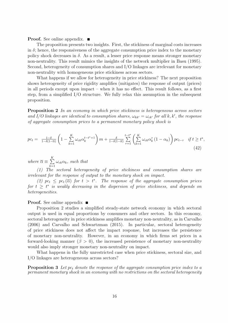
What happens if we allow for heterogeneity in price stickiness? The next propositionshows heterogeneity of price rigidity amplifies (mitigates) the response of output (prices)in all periods except upon impact – when it has no effect. This result follows, as a firststep, from a simplified I/O structure. We fully relax this assumption in the subsequentproposition.

Proposition 2 In an economy in which price stickiness is heterogeneous across sectorsand I/O linkages are identical to consumption shares, ωkk′ = ωck′ for all k, k′, the responseof aggregate consumption prices to a permanent monetary policy shock is

pct = 1−δ1−δ(1−α)

(1−

K∑k=1

ωckαt−t∗+1k

)m+ δ

1−δ(1−α)

t−t∗∑τ=1

(K∑k=1

ωckατk (1− αk)

)pct−τ if t ≥ t∗,

(42)

where α ≡K∑k=1

ωckαk, such that

(1) The sectoral heterogeneity of price stickiness and consumption shares areirrelevant for the response of output to the monetary shock on impact.

(2) pct ≤ pct (α) for t > t∗. The response of the aggregate consumption pricesfor t ≥ t∗ is weakly decreasing in the dispersion of price stickiness, and depends onheterogeneities.

Proof. See online appendixProposition 2 studies a simplified steady-state network economy in which sectoral

output is used in equal proportions by consumers and other sectors. In this economy,sectoral heterogeneity in price stickiness amplifies monetary non-neutrality, as in Carvalho(2006) and Carvalho and Schwartzman (2015). In particular, sectoral heterogeneityof price stickiness does not affect the impact response, but increases the persistenceof monetary non-neutrality. However, in an economy in which firms set prices in aforward-looking manner (β > 0), the increased persistence of monetary non-neutralitywould also imply stronger monetary non-neutrality on impact.

What happens in the fully unrestricted case when price stickiness, sectoral size, andI/O linkages are heterogeneous across sectors?

Proposition 3 Let pct denote the response of the aggregate consumption price index to apermanent monetary shock in an economy with no restrictions on the sectoral heterogeneity

16

of price stickiness αk, sectoral size ωck, and I/O linkages ωkk′. In this economy,

pct = (1− δ)

(1−

K∑k=1

ωckαt−t∗+1k

)m+ δ

t−t∗∑τ=0

K∑k=1

(K∑k′=1

ωck′ατk′ (1− αk′)ωk′k

)pkt−τ for t ≥ t∗,

(43)

with pkt−τ = 0 if t < t∗ such that(1) The response of pct is weaker on impact than in Proposition 2, when uk ≡∑K

k′=1 ωck′ (1− αk′)ωk′k > (1− α)ωck for the sectors with the stickiest prices.(2) The response of pct for t > t∗ is more persistent than in Proposition 2, when

for sectors with the stickiest prices, either of the following conditions hold: (i) ωk ≡1K

∑Kk′=1 ωk′k > ωck, (ii) uk > (1− α)ωck, (iii) COV (ωck′α

τk′ (1− αk′) , ωk′k) > 0.

Proof. See online appendix.The fully unrestricted interaction creates an even richer transmission of monetary

policy shocks. In doing so, the exact interaction of nominal and real heterogeneities iscrucial for understanding the effects of a monetary shock on output and prices. Theimplications are completely new to the literature.

First, upon impact, the price effect is weaker – and hence monetary non-neutralitylarger – than under the restricted heterogeneity of I/O linkages in Proposition 2. Thiseffect happens when the largest sectors with the stickiest prices are also importantsuppliers to the largest, most flexible sectors. Second, in subsequent periods, aggregateprice changes become more persistent given the three conditions in the second part of theproposition. In conjunction with the first result, this increased persistence means morepersistence and larger monetary non-neutrality than under restricted heterogeneity.3

In particular, a corollary of these results is a novel identity effect: The extent towhich a sector transmits monetary policy shocks depends on the exact interaction ofheterogeneity in pricing frictions and heterogeneity in sectoral size and I/O linkages. Thefollowing corollaries summarize the contribution of each sector to the path of aggregateprices, first upon impact only, and then for all subsequent periods.

Corollary 1 Upon impact, each sectoral contribution to the path of aggregate prices isgiven

(1) independently of heterogeneity in I/O linkages under homogeneous price rigidity,by [

1−(

(1− δ)(1− α)

1− δ (1− α)

)]ωckm, and (44)

(2) by a function of heterogeneities under heterogeneous price rigidity,

e′kΩc (1− δ) [I− δ (I− A) Ω]−1 (I− A) ιm, (45)

3Note we have left a contemporaneous term in the second term on the right-hand side of the propositionto make it more comparable to Proposition 2. The online appendix contains an explicit solution in termsof parameters and the monetary shock only.

17

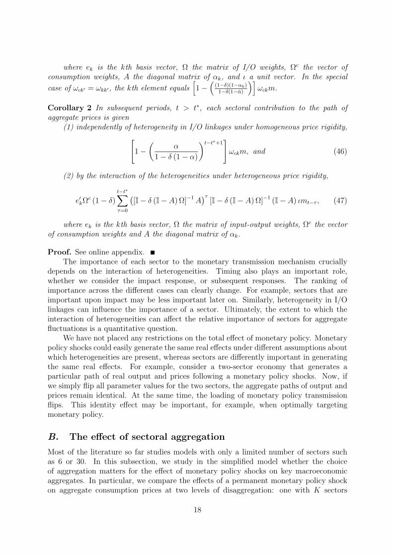
where ek is the kth basis vector, Ω the matrix of I/O weights, Ωc the vector ofconsumption weights, A the diagonal matrix of αk, and ι a unit vector. In the special

case of ωck′ = ωkk′, the kth element equals[1−

((1−δ)(1−αk)

1−δ(1−α)

)]ωckm.

Corollary 2 In subsequent periods, t > t∗, each sectoral contribution to the path ofaggregate prices is given

(1) independently of heterogeneity in I/O linkages under homogeneous price rigidity,[1−

(α

1− δ (1− α)

)t−t∗+1]ωckm, and (46)

(2) by the interaction of the heterogeneities under heterogeneous price rigidity,

e′kΩc (1− δ)

t−t∗∑τ=0

([I− δ (I− A) Ω]−1A

)τ[I− δ (I− A) Ω]−1 (I− A) ιmt−τ , (47)

where ek is the kth basis vector, Ω the matrix of input-output weights, Ωc the vectorof consumption weights and A the diagonal matrix of αk.

Proof. See online appendix.The importance of each sector to the monetary transmission mechanism crucially

depends on the interaction of heterogeneities. Timing also plays an important role,whether we consider the impact response, or subsequent responses. The ranking ofimportance across the different cases can clearly change. For example, sectors that areimportant upon impact may be less important later on. Similarly, heterogeneity in I/Olinkages can influence the importance of a sector. Ultimately, the extent to which theinteraction of heterogeneities can affect the relative importance of sectors for aggregatefluctuations is a quantitative question.

We have not placed any restrictions on the total effect of monetary policy. Monetarypolicy shocks could easily generate the same real effects under different assumptions aboutwhich heterogeneities are present, whereas sectors are differently important in generatingthe same real effects. For example, consider a two-sector economy that generates aparticular path of real output and prices following a monetary policy shocks. Now, ifwe simply flip all parameter values for the two sectors, the aggregate paths of output andprices remain identical. At the same time, the loading of monetary policy transmissionflips. This identity effect may be important, for example, when optimally targetingmonetary policy.

B. The effect of sectoral aggregation

Most of the literature so far studies models with only a limited number of sectors suchas 6 or 30. In this subsection, we study in the simplified model whether the choiceof aggregation matters for the effect of monetary policy shocks on key macroeconomicaggregates. In particular, we compare the effects of a permanent monetary policy shockon aggregate consumption prices at two levels of disaggregation: one with K sectors

18

(denoted by pct), and another in which random pairs of sectors are merged log-linearly, soit has K/2 sectors (denoted by pct). For simplicity, we assume K is even. In mathematicalterms, we compare

pct ≡K∑k=1

ωckpkt,

pct ≡K/2∑k′=1

ωck′pk′t

such that

ωck′ ≡ ωc2k′−1 + ωc2k′ ,

pk′t ≡ λk′p2k′−1 + (1− λk′) p2k′ ,

λk′ =ωc2k′−1

ωc2k′−1 + ωc2k′.

for k′ = 1, ..., K/2. This specification is without loss of generality when merging twoconsecutive sectors, because the ordering of sectors is arbitrary.

In addition, Calvo parameters are aggregated among merged sectors by

αk′ ≡ λk′α2k′−1 + (1− λk′)α2k′ .

and their I/O linkages as

ωk′s′ = ξk′ (ω2k′−1,2s′−1 + ω2k′−1,2s′) + (1− ξk′) (ω2k′,2s′−1 + ω2k′,2s′)

for k′, s′ = 1, ..., K/2. The weights ξk′ equal the shares of sectors in total intermediateinput use of the merged sectors.

First, we show that monetary non-neutrality is higher in a more disaggregatedeconomy in the absence of I/O linkages (δ = 0).

Proposition 4 When δ = 0, the difference in the response of consumption prices to apermanent monetary shock at the two levels of disaggregation is given by

pct − pct =

K/2∑k′=1

ωck′[λk′α

t−t∗+12k′−1 + (1− λk′)αt−t

∗+12k′ − αt−t∗+1

k′

]m (48)

such that (i) pct = pct for t = t∗, (ii) pct < pct for t > t∗, (iii) pct−pct is increasing in thedispersion of Calvo parameters among merged sectors, and (iv) pct − pct is increasing inthe consumption shares of merged sectors with the highest dispersion of Calvo parametersamong merged sectors.

Proof. See online appendix.This proposition is an application of Jensen’s inequality. The larger is the dispersion

in frequencies of price changes among merged sectors, the smaller is the monetary non-neutrality as the level of disaggregation becomes increasingly more coarse relative to a

19

more finely disaggregated economy. The difference in monetary non-neutrality across thetwo levels of disaggregation increases as time passes after the impact response when bothare identical. The intuition for this result is the same as in our analysis above: Aggregatingsectors overstates the response of prices to a monetary policy shock, because the measureof first-time responders is higher when the two sectors have the same frequency of pricechanges than when they exhibit different frequencies but with the same mean.

Next, we show a new result to the literature: Further disaggregation also leads tomore monetary non-neutrality by overstating the amplification introduced by intermediateinputs. We show this result under restricted heterogeneity of the production network (ωsk = ωck).

Proposition 5 When δ ∈ (0, 1) and ωsk = ωck for all s, k = 1, .., K, the difference inthe response of consumption prices to a permanent monetary shock at the two levels ofdisaggregation is given by

pct − pct =1− δ

1− δ (1− α)

K/2∑k′=1

ωck′(λk′α

t−t∗+12k′−1

+ (1− λk′ )αt−t∗+1

2k′ − αt−t∗+1

k′

)m

−δ

1− δ (1− α)

∞∑τ=1

K/2∑k′=1

ωck′

[λk′

(1− α2k′−1

)ατ2k′−1

+ (1− λk′ ) (1− α2k′ )ατ2k′

− (1− αk′ )ατk′

] pct−τ , (49)

where pct = 0 if t < t∗. Results (i) through (iv) in the previous proposition continue tohold and are amplified by the intermediate input channel.

Proof. See online appendix.Intermediate inputs introduce strategic complementarity in the response of prices to

a monetary shock, which implies consumption prices are more persistent at a finer levelof disaggregation. This effect is stronger when merged sectors with more heterogeneousfrequencies of price changes are also sectors with more homogeneous consumption shares,for a stronger short-term response of aggregate prices. The effect also increases whenmerged sectors with higher consumption shares have lower frequencies of price changes.

Third, the next proposition relaxes any restriction in the I/O structure of theproduction network. Now, the effect of aggregation on the amplification effect of monetarynon-neutrality introduced by intermediate inputs is an intricate combination of thesectoral distributions of the frequency of price changes, consumption weights, and I/Olinkages.

Proposition 6 When δ ∈ (0, 1) and I/O linkages are unrestricted, the difference inthe response of consumption prices to a permanent monetary shock at the two levels of

20

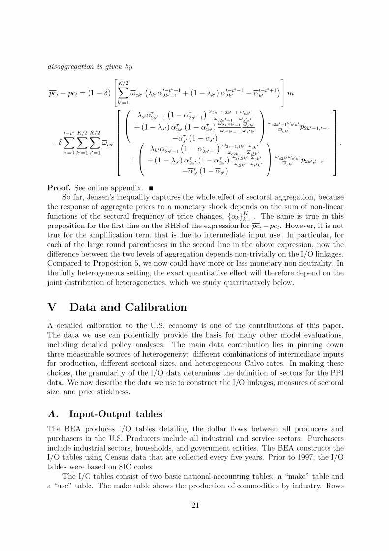
disaggregation is given by

pct − pct = (1− δ)

K/2∑k′=1

ωck′(λk′α

t−t∗+12k′−1 + (1− λk′)αt−t

∗+12k′ − αt−t∗+1

k′

)m

− δt−t∗∑τ=0

K/2∑k′=1

K/2∑s′=1

ωcs′

λs′ατ2s′−1

(1− ατ2s′−1

) ω2s−1,2k′−1

ωc2k′−1

ωck′ωs′k′

+ (1− λs′)ατ2s′ (1− ατ2s′)ω2s,2k′−1

ωc2k′−1

ωck′ωs′k′

−ατs′ (1− αs′)

ωc2k′−1ωs′k′

ωck′p2k′−1,t−τ

+

λk′ατ2s′−1

(1− ατ2s′−1

) ω2s−1,2k′

ωc2k′

ωck′ωs′k′

+ (1− λs′)ατ2s′ (1− ατ2s′)ω2s,2k′

ωc2k′

ωck′ωs′k′

−ατs′ (1− αs′)

ωc2k′ωs′k′ωck′

p2k′,t−τ

.

Proof. See online appendix.So far, Jensen’s inequality captures the whole effect of sectoral aggregation, because

the response of aggregate prices to a monetary shock depends on the sum of non-linearfunctions of the sectoral frequency of price changes, αkKk=1. The same is true in thisproposition for the first line on the RHS of the expression for pct− pct. However, it is nottrue for the amplification term that is due to intermediate input use. In particular, foreach of the large round parentheses in the second line in the above expression, now thedifference between the two levels of aggregation depends non-trivially on the I/O linkages.Compared to Proposition 5, we now could have more or less monetary non-neutrality. Inthe fully heterogeneous setting, the exact quantitative effect will therefore depend on thejoint distribution of heterogeneities, which we study quantitatively below.

V Data and Calibration

A detailed calibration to the U.S. economy is one of the contributions of this paper.The data we use can potentially provide the basis for many other model evaluations,including detailed policy analyses. The main data contribution lies in pinning downthree measurable sources of heterogeneity: different combinations of intermediate inputsfor production, different sectoral sizes, and heterogeneous Calvo rates. In making thesechoices, the granularity of the I/O data determines the definition of sectors for the PPIdata. We now describe the data we use to construct the I/O linkages, measures of sectoralsize, and price stickiness.

A. Input-Output tables

The BEA produces I/O tables detailing the dollar flows between all producers andpurchasers in the U.S. Producers include all industrial and service sectors. Purchasersinclude industrial sectors, households, and government entities. The BEA constructs theI/O tables using Census data that are collected every five years. Prior to 1997, the I/Otables were based on SIC codes.

The I/O tables consist of two basic national-accounting tables: a “make” table anda “use” table. The make table shows the production of commodities by industry. Rows

21

present industries, and columns present the commodities each industry produces. Lookingacross columns for a given row, we see all the commodities a given industry produces. Thesum of the entries comprises industry output. Looking across rows for a given column,we see all industries producing a given commodity. The sum of the entries adds up to theoutput of a commodity. The use table contains the uses of commodities by intermediateand final users. The rows in the use table contain the commodities, and the columnsshow the industries and final users that utilize them. The sum of the entries in a row isthe output of that commodity. The columns document the products each industry usesas inputs and the three components of “value added”: compensation of employees, taxeson production and imports less subsidies, and gross operating surplus. The sum of theentries in a column adds up to industry output.

We utilize the I/O tables for 2002 to create an industry network of trade flows. TheBEA defines industries at two levels of aggregation: detailed and summary accounts. Weuse both levels of aggregation to create industry-by-industry trade flows. The tables alsopin down sectoral size.

The BEA provides concordance tables between NAICS codes and I/O industry codes.We follow the BEA’s I/O classifications with minor modifications to create our industryclassifications. We account for duplicates when NAICS codes are not as detailed as I/Ocodes. In some cases, an identical set of NAICS codes defines different I/O industry codes.We aggregate industries with overlapping NAICS codes to remove duplicates.

We combine the make and use tables to construct an industry-by-industry matrix thatdetails how much of an industry’s inputs other industries produce (see online appendixfor details).

B. Price stickiness data

We use the confidential microdata underlying the producer price data (PPI) from theBLS to calculate the frequency of price adjustment at the industry level.4 The PPImeasures changes in selling prices from the perspective of producers, and tracks prices ofall goods-producing industries, such as mining, manufacturing, and gas and electricity, aswell as the service sector.5

The BLS applies a three-stage procedure to determine the sample of individual goods.In the first stage, to construct the universe of all establishments in the U.S., the BLScompiles a list of all firms filing with the Unemployment Insurance system. In the secondand third stages, the BLS probabilistically selects sample establishments and goods basedon either the total value of shipments or the number of employees. The BLS collects pricesfrom about 25,000 establishments for approximately 100,000 individual items on a monthlybasis. The BLS defines PPI prices as “net revenue accruing to a specified producingestablishment from a specified kind of buyer for a specified product shipped under specifiedtransaction terms on a specified day of the month.” Prices are collected via a survey that

4The data have been used before in Nakamura and Steinsson (2008), Goldberg and Hellerstein (2011),Bhattarai and Schoenle (2014), Gilchrist, Schoenle, Sim, and Zakrajsek (2015), Gorodnichenko and Weber(2016), Weber (2015), and D’Acunto, Liu, Pflueger, and Weber (2016).

5The BLS started sampling prices for the service sector in 2005. The PPI covers about 75% of theservice sector output. Our sample ranges from 2005 to 2011.

22

is emailed or faxed to participating establishments. Individual establishments remain inthe sample for an average of seven years until a new sample is selected to account forchanges in the industry structure.

We calculate the frequency of price changes at the goods level, FPA, as the ratio ofthe number of price changes to the number of sample months. For example, if an observedprice path is $10 for two months and then $15 for another three months, one price changeoccurs during five months, and the frequency is 1/5. We aggregate goods-based frequenciesto the BEA industry classification.

The overall mean monthly frequency of price adjustment is 16.78%, which impliesan average duration, −1/ log(1 − FPA), of 6.15 months. Substantial heterogeneity ispresent in the frequency across sectors, ranging from as low as 4.01% for the semiconductormanufacturing sector (duration of 56.26 months) to 93.75% for dairy production (durationof 0.83 months).

C. Parameter Calibration

We calibrate our model at different levels of detail to analyze monetary non-neutrality.One contribution is the calibration of a highly disaggregated 341-sector economy, whichwe discuss in section VI, and contrast key results with more aggregated economies.

We calibrate the model at the monthly frequency using standard parameter values inthe literature (see Table 1). The coefficient of relative risk aversion σ is 1, and β = 0.9975,implying an annual risk-free interest rate of 3%. We set ϕ = 2, implying a Frisch elasticityof labor supply of 0.5. We set δ, the average share of inputs in the production function, to0.5, in line with Basu (1995) and empirical estimates. We set the within-sector elasticity ofsubstitution θ to 6, implying a steady-state markup of 20%, and the across-sector elasticityof substitution η to 2, in line with Carvalho and Lee (2011). We set the parameters inthe Taylor rule to standard values of φπ = 1.24 and φc = 0.33/12 (see Rudebusch (2002))with a persistence parameter of monetary shocks of ρ = 0.9. We also study a calibrationwith interest rate smoothing as in Coibion and Gorodnichenko (2012).6

We investigate the robustness of our findings to permutations in parameter values insection IV of the online appendix. Overall, the main conclusions remain unaffected byvariations in assumptions.

VI Quantitative Results

We now study the importance of different heterogeneities for the real effects of monetaryshocks in detailed calibration of the model, for the identity of the sectors that are thebiggest contributors to real effects, and how sectoral aggregation affects real effects ofmonetary policy shocks.

6When Coibion and Gorodnichenko (2012) estimate a Taylor rule without interest rate smooth butpersistent shocks, they find estimates of the autoregressive parameter of monetary policy shocks equal to0.96.

23

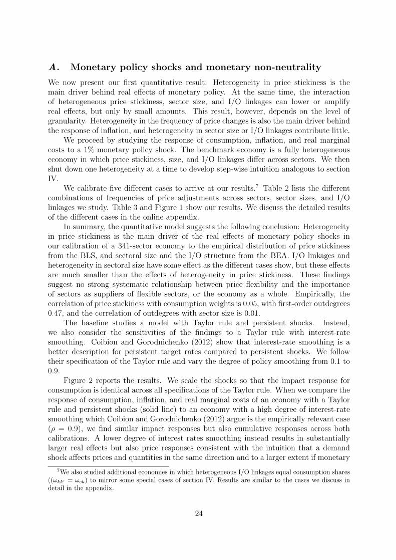
A. Monetary policy shocks and monetary non-neutrality

We now present our first quantitative result: Heterogeneity in price stickiness is themain driver behind real effects of monetary policy. At the same time, the interactionof heterogeneous price stickiness, sector size, and I/O linkages can lower or amplifyreal effects, but only by small amounts. This result, however, depends on the level ofgranularity. Heterogeneity in the frequency of price changes is also the main driver behindthe response of inflation, and heterogeneity in sector size or I/O linkages contribute little.

We proceed by studying the response of consumption, inflation, and real marginalcosts to a 1% monetary policy shock. The benchmark economy is a fully heterogeneouseconomy in which price stickiness, size, and I/O linkages differ across sectors. We thenshut down one heterogeneity at a time to develop step-wise intuition analogous to sectionIV.

We calibrate five different cases to arrive at our results.7 Table 2 lists the differentcombinations of frequencies of price adjustments across sectors, sector sizes, and I/Olinkages we study. Table 3 and Figure 1 show our results. We discuss the detailed resultsof the different cases in the online appendix.

In summary, the quantitative model suggests the following conclusion: Heterogeneityin price stickiness is the main driver of the real effects of monetary policy shocks inour calibration of a 341-sector economy to the empirical distribution of price stickinessfrom the BLS, and sectoral size and the I/O structure from the BEA. I/O linkages andheterogeneity in sectoral size have some effect as the different cases show, but these effectsare much smaller than the effects of heterogeneity in price stickiness. These findingssuggest no strong systematic relationship between price flexibility and the importanceof sectors as suppliers of flexible sectors, or the economy as a whole. Empirically, thecorrelation of price stickiness with consumption weights is 0.05, with first-order outdegrees0.47, and the correlation of outdegrees with sector size is 0.01.

The baseline studies a model with Taylor rule and persistent shocks. Instead,we also consider the sensitivities of the findings to a Taylor rule with interest-ratesmoothing. Coibion and Gorodnichenko (2012) show that interest-rate smoothing is abetter description for persistent target rates compared to persistent shocks. We followtheir specification of the Taylor rule and vary the degree of policy smoothing from 0.1 to0.9.

Figure 2 reports the results. We scale the shocks so that the impact response forconsumption is identical across all specifications of the Taylor rule. When we compare theresponse of consumption, inflation, and real marginal costs of an economy with a Taylorrule and persistent shocks (solid line) to an economy with a high degree of interest-ratesmoothing which Coibion and Gorodnichenko (2012) argue is the empirically relevant case(ρ = 0.9), we find similar impact responses but also cumulative responses across bothcalibrations. A lower degree of interest rates smoothing instead results in substantiallylarger real effects but also price responses consistent with the intuition that a demandshock affects prices and quantities in the same direction and to a larger extent if monetary

7We also studied additional economies in which heterogeneous I/O linkages equal consumption shares((ωkk′ = ωck) to mirror some special cases of section IV. Results are similar to the cases we discuss indetail in the appendix.

24

policy does not buffer the shock.

B. Heterogeneity across sectors, and identity effects

So far, we find heterogeneous price stickiness is the key driver behind large effects ofmonetary policy shocks, whereas heterogeneous sector size or I/O linkages seem to play asecondary role. We will see below, however, that such a conclusion would be premature.Our analysis shows substantial heterogeneity in the sectoral responses to the common,monetary policy shock. Which sector transmits the monetary policy shock the mostdepends crucially on our specification of heterogeneities. This finding presents anothernew and important result of the paper, especially for policymakers. Heterogeneity inmarkup responses reflects heterogeneity in real output and identity effects.

We present these results by focusing on the 10 most and least contractionary sectoraloutput contributors to real output effects of monetary shocks. Table 4 reports therespective cumulative real effects of monetary policy shocks in Panels A and B for ourdifferent cases.

We know from the discussion in section IV that all sectors are equally responsive inmodels with homogeneous flexible or sticky prices. The actual response in an economy inwhich sectors differ in their degree of price stickiness, sector size, and I/O linkages differsmarkedly across sectors. We see in Table A that the 10 least responsive contractionarysectors have a large and positive response to a contractionary monetary policy shock.The positive response can happen if these sectors are substantially more flexible than theaverage sector in the data which is indeed the case. Sectors with a positive consumptionresponse have an average frequency of price adjustment that is larger by a factor of 3relative to the average sector. In panel B, instead, we see very large negative responsesamong the 10 most responsive sectors to a contractionary shock.

We see in column (2) and (3) that shutting down either heterogeneity in sector sizeor I/O linkages reduces the effective granularity substantially. Both in panel A and B,we see a large compression in the responses. The most responsive sectors in columns (2)and (3) respond by only 25% of the response of the most responsive sector in column (1)with all heterogeneities presents and the range of the responses between sector 1 and 10shrinks by a factor of 5.

When we shut down both heterogeneity in sector size and I/O linkages and onlyfocus on differences in price stickiness across sectors, we see an additional compressionto the mean both among the least and most responsive sectors. When we compare theresponse across columns (1) to (4), we see (i) heterogeneous price stickiness is central for adifferential response across sectors to a common monetary policy shock; (ii) heterogeneityin sector size and I/O linkages by themselves add to the granularity of the economyrelative to column (4); (iii) it is the inter-linkages between heterogeneity in sector size,price stickiness, and I/O linkages that have a big effects on the contribution of the mostand least responsive sectors to a common monetary policy shock.

The results in Table 4 show that the intricacies in which different heterogeneitiesinteract play a crucial role for the relative contribution of different sectors to the aggregatereal effects of monetary policy. Purely focusing on the average impact and cumulativeeffects masks substantial heterogeneity across sectoral responses and policy makers that

25

would aim to stabilize certain sectors would possibly commit policy mistakes by onlyfocusing on the heterogeneity in price stickiness across sections which is a classical resultin the literature (see Aoki (2001)).

Figure 3 graphically illustrates the identity effects across all 341 sectors when we gofrom case 1 in which all heterogeneities are present to case 4 with only heterogeneousprice stickiness across sectors. Rankings change substantially across sectors with somesectors changing up to 300 ranks. Hence, the exact choice of heterogeneities is clearlyimportant for the identity of sectors in the transmission mechanism.

Heterogeneity in markups reflects the heterogeneity in real output effects. Pricemarkups are of independent importance and interest, because they measure theinefficiency in the economy and are equivalent to a countercyclical labor wedge (see Galiet al. (2007)). In our setting, the product market wedge is the sole driver of the laborwedge which is consistent with recent empirical work by Bils, Klenow, and Malin (2014).8

The level of markups in the full model is higher than in the homogeneous benchmarkcase, and markups display a rich, dynamic pattern. We report these findings in FigureA.1 of the online appendix.

The effect of fully interacted heterogeneities in our model becomes clear in comparisonto the completely homogeneous economy. The markup responses of the homogeneouseconomy are summarized in Panel (a) of Figure A.1 in the online appendix. All sectoralresponses are fast-decaying and identical across all percentiles. The markup response ismore than 4.5% on impact, with a half-life of eight periods.

By contrast, two differential facts emerge for the full model (case 1): First, the mediansectoral response is substantially larger. The initial median markup response increasesto approximately 6%. The dashed, thick blue line summarizes the median response. Thehalf-life of the median response is twice as long as in the homogeneous case.

Second, substantial dispersion exists in the markup response. The top 5th percentileof markups increases to over 10%; the bottom 5th percentile does not increase above 4%.The sectoral markups also show very different dynamic patterns: The top percentilesshow a hump-shaped response that is very persistent, with a half-life of more than 15periods. At the same time, the lowest percentiles decay exponentially with a half-life ofless than ten periods. These very different price-markup responses directly result fromthe convolutions of the different underlying heterogeneities. They open up new avenuesto study how interactions of different heterogeneities shape inefficiencies in the economy.

C. Sectoral Aggregation and Real Effects

In this section, we study the response of our model economy to monetary policy shocks fordifferent levels of disaggregation keeping constant the average degree of price stickinessacross levels of aggregation. The choice of aggregation results in large differences in realeffects across model economies. We arrive at this conclusion in two steps.

First, we compare the two levels of granularity published by the BEA: detail(effectively 341 sectors), summary (56 sectors), and an even coarser aggregation withonly 7 sectors. The left panel of Figure 4 and Table 5 report our findings. Cumulative

8Shimer (2009) stresses the lack of work on heterogeneity in the product market, a channel we areputting forward and expanding upon by allowing for interactions of different heterogeneities.

26

real effects of monetary policy are 6% larger in the more disaggregated 341-sector economythan in the 56-sector calibration but almost 50% larger than in an economy with only7 sectors which has been the approximate number of sectors in many calibrations in theliterature.

The inflation response is interesting: Upon impact, the inflation response is verysimilar across different levels of disaggregation, whereas already large differences exists inthe consumption response across calibrations. Moreover, the inflation response of the 56sector economy is larger on impact than the response for the 7 sector economy but theconsumption response on impact is also larger for the more disaggregated model. Thisfinding cautions against drawing inference for monetary policy from the impact responseof inflation to monetary policy shocks.

Second, motivated by these findings as well as our theoretical results in section IV– that the degree of granularity can matter for the real effects of monetary policy – wenow systematically show the importance of granularity when we aggregate sectors by sizeinstead of following the BEA aggregation.

In many models, sector size is a good proxy for sector technology. The right panelof Figure 4 and Table A.1in the online appendix show the results. The real effects ofmonetary policy are now dramatically affected. They are more than 40% larger on impactfor the most disaggregated economy compared to the less disaggregated economy withonly 56 sectors, even though the impact response of inflation is again similar. Realeffects are monotonically increasing in the granularity of the economy. Figure A.2 in theonline appendix shows the dispersion in the frequency of price adjustment shrinks for lessgranular economies.

What mechanisms are driving these aggregation effects? We find the interactions ofheterogeneities are more important than the convexification of price rigidities in creatingaggregation effects, but they act with some delay. We show the relative importance bycomputing the total consumption price paths in a 341 and an 7 sector economy, as well asthe two components from equation (43), due to convexification and interactions. FigureA.3 in the online appendix illustrates how the two channels contribute to the total gap.

VII Concluding Remarks

We present new theoretical and quantitative insights into the transmission of monetarypolicy shocks when heterogeneity in price stickiness, the I/O structure, and sector sizeinteract.

Although rich theoretical predictions exist for how the interaction of theseheterogeneities shapes the real output effects of monetary shocks, we find in our calibrationto the US economy that heterogeneity in price stickiness is the central mechanism forgenerating large and persistent real output effects. Heterogeneity in I/O linkages, instead,only plays a marginal role. In addition, we document that small-scale models mightsubstantially underestimate output effects – even though the impact response of inflationis almost identical across different levels of granularity. We also find that heterogeneity inprice rigidity is key in determining which sectors are the most important contributors tothe transmission of monetary shocks. Finally, while heterogeneity in sector size and I/O

27

linkages only play a minor role in shaping the aggregate real output effects of monetaryshocks, we find that they jointly increase the effective granularity in the economy.

Our results have important policy implications. First, the impact response of inflationto a monetary policy shock is not sufficient for the real effects of monetary shocks. Second,the real effects of more granular economies are substantially larger compared to economieswith only a small number of sectors. And finally, all heterogeneities we study areimportant for the identity and contribution of the most important sectors to the real effectsof monetary policy. In particular, sectoral price stickiness is not the only determinant forthe contribution to aggregate real effects. Despite mattering only marginally for the overallreal effects, heterogeneity in sector size and I/O linkages are important contributors andgenerate an increase in the effective granularity: the most important sectors contributingto aggregate real effects become even more important, whereas the least important sectorsbecome even less important. The latter result suggest that central bank should no longeronly focus on stabilizing the prices of the most sticky-price sectors but should jointly focuson the interaction of sector size, I/O linkages, and price stickiness.

While we study a rich set of heterogeneities at the sectoral level that are we candirectly map into data, we leave out other important differences such as the degree ofdurability, differences in intermediate input shares, or heterogeneity in the elasticitiesof demand. We hypothesize that more downstream sectors with stickier prices mightalso produce more durable goods compared to commodities sectors with flexible pricesand higher elasticities of demand which would possibly amplify real output effects ofmonetary shocks. We believe these heterogeneities are important to study but leave adetailed analysis to future research.

28

References

Acemoglu, D., U. Akcigit, and W. Kerr (2015). Networks and the macroeconomy: Anempirical exploration. NBER Macroeconomics Annual .

Acemoglu, D., V. M. Carvalho, A. Ozdaglar, and A. Tahbaz-Salehi (2012). The networkorigins of aggregate fluctuations. Econometrica 80 (5), 1977–2016.

Alvarez, F. E., F. Lippi, and L. Paciello (2016). Monetary shocks in models withinattentive producers. The Review of Economic Studies 83 (2), 421–459.

Aoki, K. (2001). Optimal monetary policy responses to relative-price changes. Journal ofmonetary economics 48 (1), 55–80.

Barrot, J.-N. and J. Sauvagnat (2016). Input specificity and the propagation ofidiosyncratic shocks in production networks. The Quarterly Journal of Economics ,1543–1592.

Basu, S. (1995). Intermediate goods and business cycles: Implications for productivityand welfare. The American Economic Review 85 (3), 512–531.

Bhattarai, S. and R. Schoenle (2014). Multiproduct firms and price-setting: Theory andevidence from U.S. producer prices. Journal of Monetary Economics 66, 178–192.

Bigio, S. and J. La’O (2017). Financial frictions in production networks. UnpublishedManuscript, Columbia University .

Bils, M., P. J. Klenow, and B. A. Malin (2014). Resurrecting the role of the product marketwedge in recessions. NBER Working Papers 20555, National Bureau of EconomicResearch.

Boivin, J., M. P. Giannoni, and I. Mihov (2009). Sticky prices and monetary policy:Evidence from disaggregated U.S. data. The American Economic Review 99 (1), 350–384.

Bouakez, H., E. Cardia, and F. Ruge-Murcia (2014). Sectoral price rigidity and aggregatedynamics. European Economic Review 65, 1–22.

Calvo, G. A. (1983). Staggered prices in a utility-maximizing framework. Journal ofMonetary Economics 12 (3), 383–398.

Carvalho, C. (2006). Heterogeneity in price stickiness and the real effects of monetaryshocks. The B.E. Journal of Macroeconomics 6 (3), 1–56.

Carvalho, C. and J. W. Lee (2011). Sectoral price facts in a sticky-price model.Unpublished Manuscript, PUC-Rio.

Carvalho, C. and F. Schwartzman (2015). Selection and monetary non-neutrality intime-dependent pricing models. Journal of Monetary Economics 76, 141–156.

Carvalho, V. M. (2014). From micro to macro via production networks. The Journal ofEconomic Perspectives 28 (4), 23–47.

Coibion, O. and Y. Gorodnichenko (2012). Why are target interest rate changes sopersistent? American Economic Journal: Macroeconomics 4 (4), 126–162.

Cox, L., G. Mueller, E. Pasten, R. Schoenle, and M. Weber (2019). Big G. Unpublishedmanuscript, University of Chicago.

D’Acunto, F., R. Liu, C. Pflueger, and M. Weber (2016). Flexible prices and leverage.Unpublished manuscript, University of Chicago.

29

Gabaix, X. (2011). The granular origins of aggregate fluctuations. Econometrica 79 (3),733–772.

Gali, J., M. Gertler, and J. D. Lopez-Salido (2007). Markups, gaps, and the welfare costsof business fluctuations. The Review of Economics and Statistics 89 (1), 44–59.

Gilchrist, S., R. Schoenle, J. Sim, and E. Zakrajsek (2015). Inflation dynamics during theFinancial Crisis. Unpublished Manuscript, Brandeis University .

Goldberg, P. P. and R. Hellerstein (2011). How rigid are producer prices? FRB of NewYork Staff Report , 1–55.

Gorodnichenko, Y. and M. Weber (2016). Are sticky prices costly? Evidence from thestock market. American Economic Review 106 (1), 165–199.

Herskovic, B. (2018). Networks in production: Asset pricing implications. The Journalof Finance 73 (4), 1785–1818.

Herskovic, B., B. T. Kelly, H. Lustig, and S. Van Nieuwerburgh (2016). The commonfactor in idiosyncratic volatility: Quantitative asset pricing implications. Journal ofFinancial Economics 119 (2), 249–283.

Huang, K. X. D. and Z. Liu (2001). Production chains and general equilibrium aggregatedynamics. Journal of Monetary Economics 48 (2), 437–462.

Huang, K. X. D. and Z. Liu (2004). Input–output structure and nominal rigidity: Thepersistence problem revisited. Macroeconomic Dynamics 8 (2), 188–206.

Kelly, B., H. Lustig, and S. Van Nieuwerburgh (2013). Firm volatility in granularnetworks. NBER Working Papers 19466, National Bureau of Economic Research.

Lucas, R. E. (1977). Understanding business cycles. In Carnegie-Rochester conferenceseries on public policy, Volume 5, pp. 7–29. Elsevier.

Nakamura, E. and J. Steinsson (2008). Five facts about prices: A reevaluation of menucost models. The Quarterly Journal of Economics 123 (4), 1415–1464.

Nakamura, E. and J. Steinsson (2010). Monetary non-neutrality in a multi-sector menucost model. The Quarterly Journal of Economics 125 (3), 961–1013.

Ozdagli, A. and M. Weber (2017). Monetary policy through production networks:Evidence from the stock market. Unpublished Manuscript, University of Chicago.

Pasten, E., R. Schoenle, and M. Weber (2018). Price rigidity and the origins of aggregatefluctuations. Unpublished manuscript, University of Chicago.

Rudebusch, G. D. (2002). Term structure evidence on interest rate smoothing andmonetary policy inertia. Journal of Monetary Economics 49 (6), 1161–1187.

Shamloo, M. (2010). Price setting in a model with production chains: Evidence fromsectoral data. IMF Working Papers 10 (82), 1–50.

Shimer, R. (2009). Convergence in macroeconomics: The labor wedge. AmericanEconomic Journal: Macroeconomics 1 (1), 280–297.

Weber, M. (2015). Nominal rigidities and asset pricing. Unpublished manuscript,University of Chicago Booth School of Business .

30

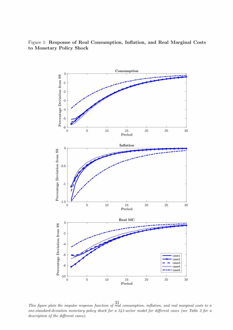
Figure 1: Response of Real Consumption, Inflation, and Real Marginal Coststo Monetary Policy Shock

0 5 10 15 20 25 30-6

-5

-4

-3

-2

-1

0

0 5 10 15 20 25 30-1.5

-1

-0.5

0

0 5 10 15 20 25 30-10

-8

-6

-4

-2

0

case1case2case3case4case5

This figure plots the impulse response function of real consumption, inflation, and real marginal costs to a

one-standard-deviation monetary policy shock for a 341-sector model for different cases (see Table 2 for a

description of the different cases).

31

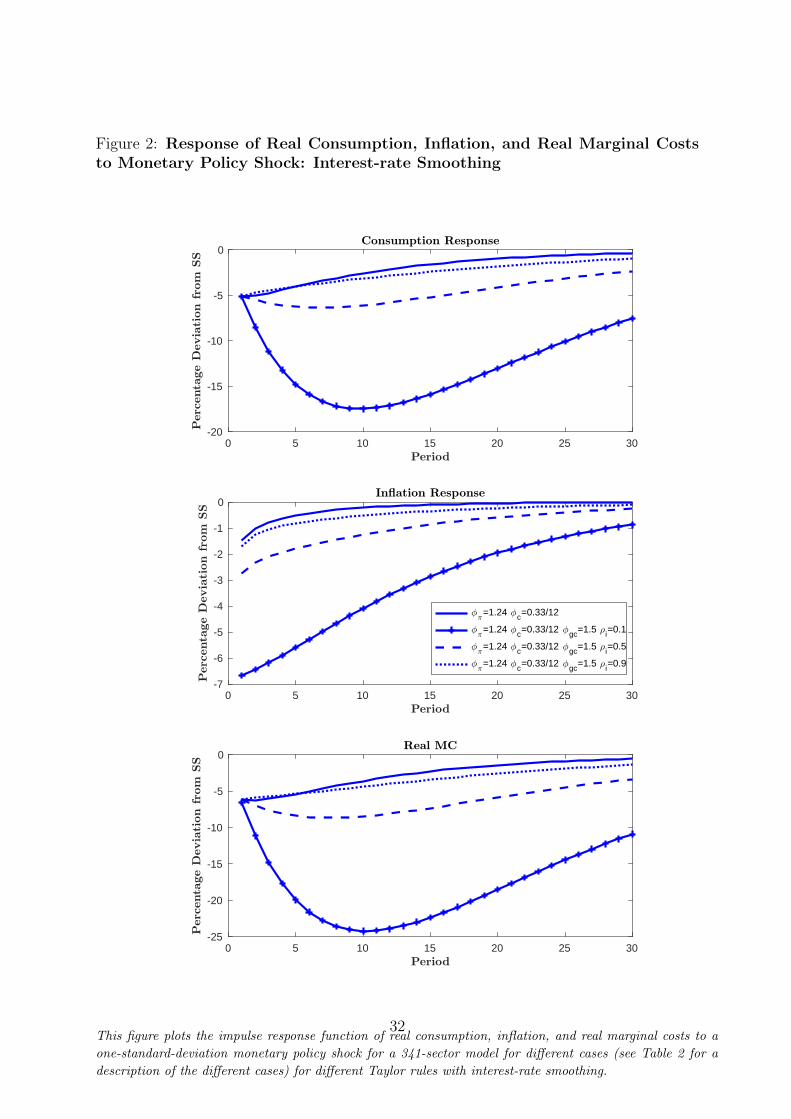
Figure 2: Response of Real Consumption, Inflation, and Real Marginal Coststo Monetary Policy Shock: Interest-rate Smoothing

0 5 10 15 20 25 30-20

-15

-10

-5

0

0 5 10 15 20 25 30-7

-6

-5

-4

-3

-2

-1

0

=1.24 c=0.33/12

=1.24 c=0.33/12 gc=1.5 i=0.1

=1.24 c=0.33/12 gc=1.5 i=0.5

=1.24 c=0.33/12 gc=1.5 i=0.9

0 5 10 15 20 25 30-25

-20

-15

-10

-5

0

This figure plots the impulse response function of real consumption, inflation, and real marginal costs to a

one-standard-deviation monetary policy shock for a 341-sector model for different cases (see Table 2 for a

description of the different cases) for different Taylor rules with interest-rate smoothing.

32

Figure 3: Ranking of Sectors, Cases 1 and 4

0 50 100 150 200 250 300 3500

50

100

150

200

250

300

350

This figure plots the sectoral rankings for the cumulative IRF for case 1 against case 4 (see Table 2 for a

description of the different cases).

33

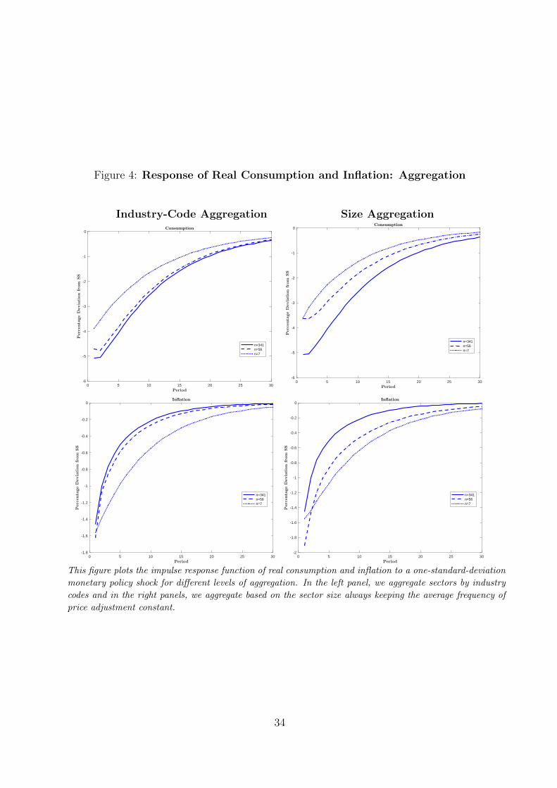
Figure 4: Response of Real Consumption and Inflation: Aggregation

Industry-Code Aggregation Size Aggregation

0 5 10 15 20 25 30-6

-5

-4

-3

-2

-1

0

n=341n=56n=7

0 5 10 15 20 25 30-6

-5

-4

-3

-2

-1

0

n=341n=56n=7

0 5 10 15 20 25 30-1.8

-1.6

-1.4

-1.2

-1

-0.8

-0.6

-0.4

-0.2

0

n=341n=56n=7

0 5 10 15 20 25 30-2

-1.8

-1.6

-1.4

-1.2

-1

-0.8

-0.6

-0.4

-0.2

0

n=341n=56n=7

This figure plots the impulse response function of real consumption and inflation to a one-standard-deviation

monetary policy shock for different levels of aggregation. In the left panel, we aggregate sectors by industry

codes and in the right panels, we aggregate based on the sector size always keeping the average frequency of

price adjustment constant.

34

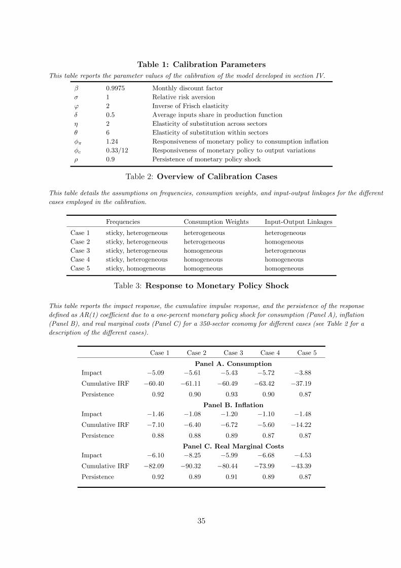
Table 1: Calibration Parameters

This table reports the parameter values of the calibration of the model developed in section IV.

β 0.9975 Monthly discount factor

σ 1 Relative risk aversion

ϕ 2 Inverse of Frisch elasticity

δ 0.5 Average inputs share in production function

η 2 Elasticity of substitution across sectors

θ 6 Elasticity of substitution within sectors

φπ 1.24 Responsiveness of monetary policy to consumption inflation

φc 0.33/12 Responsiveness of monetary policy to output variations

ρ 0.9 Persistence of monetary policy shock

Table 2: Overview of Calibration Cases

This table details the assumptions on frequencies, consumption weights, and input-output linkages for the different

cases employed in the calibration.

Frequencies Consumption Weights Input-Output Linkages

Case 1 sticky, heterogeneous heterogeneous heterogeneous

Case 2 sticky, heterogeneous heterogeneous homogeneous

Case 3 sticky, heterogeneous homogeneous heterogeneous

Case 4 sticky, heterogeneous homogeneous homogeneous

Case 5 sticky, homogeneous homogeneous homogeneous

Table 3: Response to Monetary Policy Shock

This table reports the impact response, the cumulative impulse response, and the persistence of the response

defined as AR(1) coefficient due to a one-percent monetary policy shock for consumption (Panel A), inflation

(Panel B), and real marginal costs (Panel C) for a 350-sector economy for different cases (see Table 2 for a

description of the different cases).

Case 1 Case 2 Case 3 Case 4 Case 5

Panel A. Consumption

Impact −5.09 −5.61 −5.43 −5.72 −3.88

Cumulative IRF −60.40 −61.11 −60.49 −63.42 −37.19

Persistence 0.92 0.90 0.93 0.90 0.87

Panel B. Inflation

Impact −1.46 −1.08 −1.20 −1.10 −1.48

Cumulative IRF −7.10 −6.40 −6.72 −5.60 −14.22

Persistence 0.88 0.88 0.89 0.87 0.87

Panel C. Real Marginal Costs

Impact −6.10 −8.25 −5.99 −6.68 −4.53

Cumulative IRF −82.09 −90.32 −80.44 −73.99 −43.39

Persistence 0.92 0.89 0.91 0.89 0.87

35

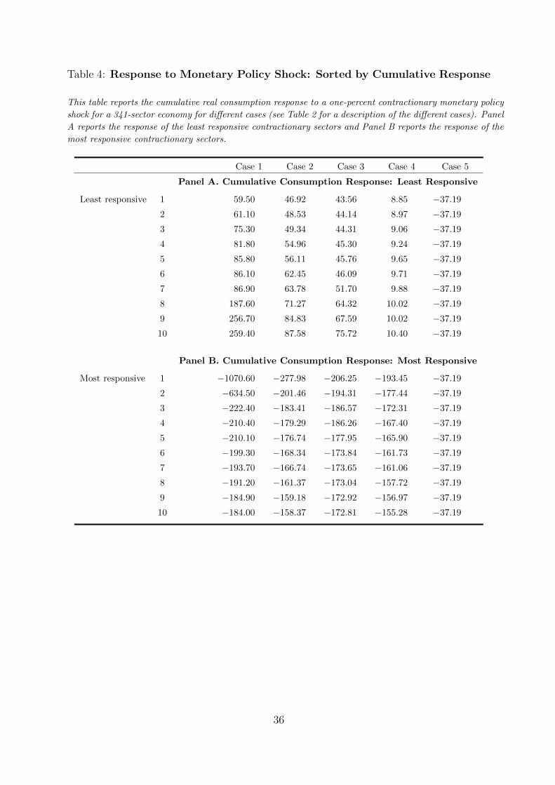
Table 4: Response to Monetary Policy Shock: Sorted by Cumulative Response

This table reports the cumulative real consumption response to a one-percent contractionary monetary policy

shock for a 341-sector economy for different cases (see Table 2 for a description of the different cases). Panel

A reports the response of the least responsive contractionary sectors and Panel B reports the response of the

most responsive contractionary sectors.

Case 1 Case 2 Case 3 Case 4 Case 5

Panel A. Cumulative Consumption Response: Least Responsive

Least responsive 1 59.50 46.92 43.56 8.85 −37.19

2 61.10 48.53 44.14 8.97 −37.19

3 75.30 49.34 44.31 9.06 −37.19

4 81.80 54.96 45.30 9.24 −37.19

5 85.80 56.11 45.76 9.65 −37.19

6 86.10 62.45 46.09 9.71 −37.19

7 86.90 63.78 51.70 9.88 −37.19

8 187.60 71.27 64.32 10.02 −37.19

9 256.70 84.83 67.59 10.02 −37.19

10 259.40 87.58 75.72 10.40 −37.19

Panel B. Cumulative Consumption Response: Most Responsive

Most responsive 1 −1070.60 −277.98 −206.25 −193.45 −37.19

2 −634.50 −201.46 −194.31 −177.44 −37.19

3 −222.40 −183.41 −186.57 −172.31 −37.19

4 −210.40 −179.29 −186.26 −167.40 −37.19

5 −210.10 −176.74 −177.95 −165.90 −37.19

6 −199.30 −168.34 −173.84 −161.73 −37.19

7 −193.70 −166.74 −173.65 −161.06 −37.19

8 −191.20 −161.37 −173.04 −157.72 −37.19

9 −184.90 −159.18 −172.92 −156.97 −37.19

10 −184.00 −158.37 −172.81 −155.28 −37.19

36

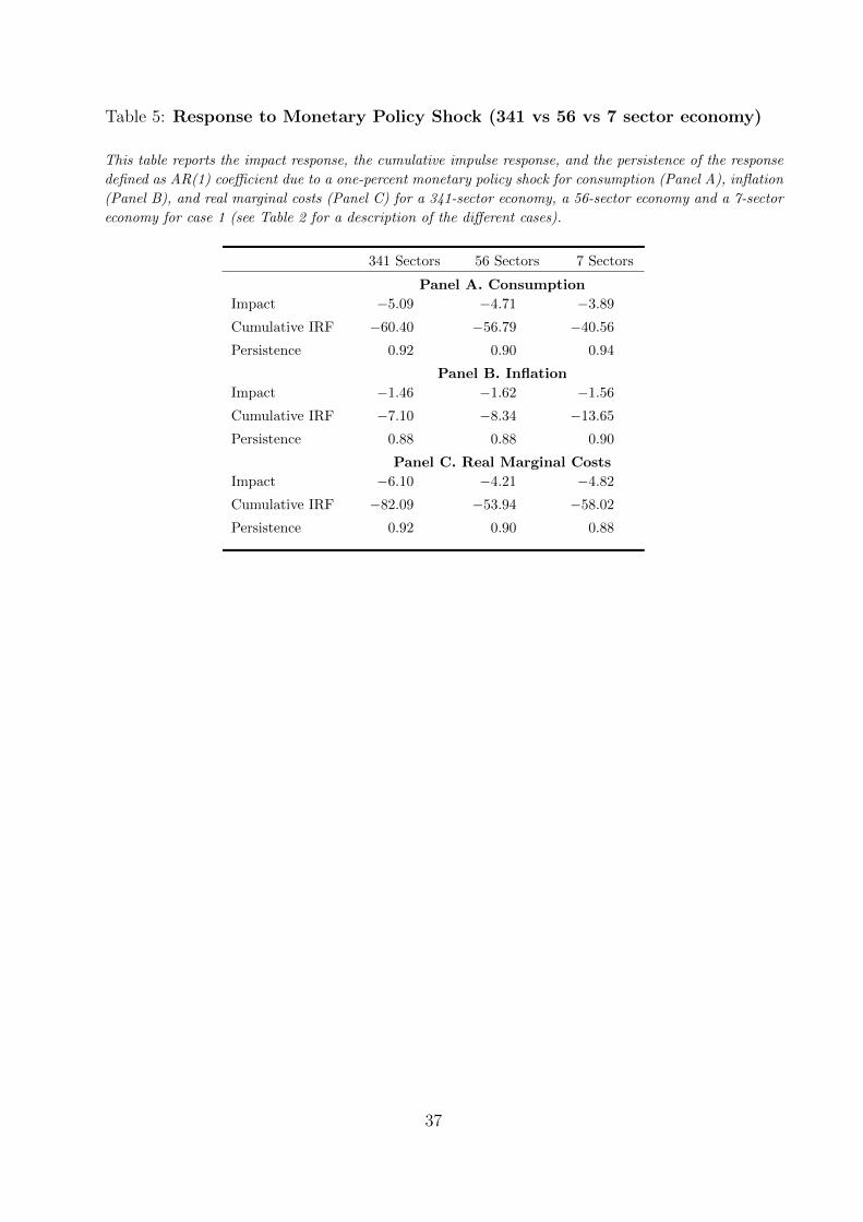
Table 5: Response to Monetary Policy Shock (341 vs 56 vs 7 sector economy)

This table reports the impact response, the cumulative impulse response, and the persistence of the response

defined as AR(1) coefficient due to a one-percent monetary policy shock for consumption (Panel A), inflation

(Panel B), and real marginal costs (Panel C) for a 341-sector economy, a 56-sector economy and a 7-sector

economy for case 1 (see Table 2 for a description of the different cases).

341 Sectors 56 Sectors 7 Sectors

Panel A. Consumption

Impact −5.09 −4.71 −3.89

Cumulative IRF −60.40 −56.79 −40.56

Persistence 0.92 0.90 0.94

Panel B. Inflation

Impact −1.46 −1.62 −1.56

Cumulative IRF −7.10 −8.34 −13.65

Persistence 0.88 0.88 0.90

Panel C. Real Marginal Costs

Impact −6.10 −4.21 −4.82

Cumulative IRF −82.09 −53.94 −58.02

Persistence 0.92 0.90 0.88

37