Electronic copy available at: http://ssrn.com/abstract=2021301

Propagation of Financial Shocks:

The Case of Venture Capital

⇤

Richard R. Townsend†

October 29, 2012

Abstract

This paper investigates how venture-backed companies are affected when oth-ers sharing the same investor perform poorly. I show that in theory companiesmay be helped or hurt. Empirically, I estimate the impact of the technology bub-ble’s collapse on non-information-technology companies held alongside internetcompanies in venture portfolios. I find the collapse was associated with a 26%larger decline in the probability of raising additional financing for these non-IT companies compared with others. I control for unobservable characteristicsby examining companies with multiple investors. The results suggest that theseemingly robust structure of venture intermediaries does not eliminate/reversecontagion among portfolio companies.

JEL Classification: G11, G24

Key Words: Intermediation, Contagion, Venture Capital, Technology Bubble, Internet, Lock-in

⇤I am deeply grateful to Paul Gompers, Josh Lerner, Andrei Shleifer, and Jeremy Stein for their invaluableguidance and encouragement throughout this project. I also thank Malcolm Baker, Shai Bernstein, SudheerChava, Sergey Chernenko, Joshua Coval, Hongyi Li, Ramana Nanda, David Scharfstein, Antoinette Schoar,Josh Schwartzstein, Adi Sunderam, and Thomas Wang for extremely helpful comments and suggestions.This paper also benefited greatly from comments of seminar participants at Dartmouth College (Tuck),The Federal Reserve Board, Harvard University, Indiana University (Kelley), London School of Economics,Northwestern University (Kellogg), University of Notre Dame (Mendoza), Rochester University (Simon),University of North Carolina (Kenan-Flagler), and the Kauffman Entrepreneurial Finance and InnovationConference.

†Tuck School of Business, Dartmouth College, 100 Tuck Hall, Hanover, NH 03755. Phone: 603-646-8965.Fax: 603-646-0995. E-Mail: richard.r.townsend@tuck.dartmouth.edu.

Electronic copy available at: http://ssrn.com/abstract=2021301

1 Introduction

The structure of venture capital investment firms (henceforth “venture firms” or “venture

investors”) differs from that of other intermediaries in several ways that ostensibly make

them less fragile and more self-contained. First, investors in a venture fund are required to

commit capital for the entire life of the fund (typically 10 years), thus there are no issues

of maturity mismatch in assets and liabilities. Second, venture firms are often limited in

the extent to which they can invest in the same company out of multiple funds under their

management. In this paper, I examine the impact of this unique intermediation structure

on portfolio companies. In particular, I examine how companies’ access to capital is affected

when the prospects of others held in the same portfolio decline.

I demonstrate in a simple model that it is ambiguous whether companies would be helped

or hurt in this scenario, given the institutional features just described. On the one hand,

after a negative shock to some companies in a venture portfolio, unrelated companies would

become more attractive in relative terms. All else equal, this would make it easier for them to

obtain continuation financing. This relates closely to the “bright side” view of internal capital

markets, in which corporate headquarters engages in relative evaluation (Stein, 1997). On the

other hand, a venture investment firm with high exposure to the shock may experience more

difficulty raising new funds from limited partners. I show that if venture firm fundraising

is sufficiently sensitive to interim performance, this can make it more difficult for portfolio

companies unrelated to the shock to obtain continuation financing. This turns out to be

true even if there are cross-fund investing restrictions prohibiting new funds from being

invested in existing portfolio companies. Thus, the direction of contagion (reverse contagion

vs. ordinary contagion) among venture-backed portfolio companies is ultimately an empirical

question. Knowing the answer to this would improve not only our understanding of venture

capital, but of financial intermediation more broadly. In particular, if ordinary contagion

1

Electronic copy available at: http://ssrn.com/abstract=2021301

occurs even in the absence of maturity mismatch, this may be informative when considering

policies to reduce the fragility of other intermediaries.

In terms of the venture capital setting specifically, it is also true that contagion would

likely be of particular consequence in this context. Indeed, for mature companies, disrup-

tions in intermediary relationships may be harmful but survivable. By contrast, for typical

venture-backed companies, with negative earnings and few tangible assets, these disruptions

are much more likely to lead to company failure. Moreover, such failures are especially im-

portant given the nature of the companies financed by venture firms. Many of the largest

companies in the U.S. by market capitalization, including Apple, Google, Microsoft, and

Cisco, were backed by venture firms in their early days. In addition, more than 60% of the

IPOs that have occurred since 1999 have been venture-backed (Kaplan and Lerner, 2010).

Given that venture firms provide capital to highly innovative companies with the potential

to create large social surpluses, distortions in their capital allocation decisions could have

important welfare implications.

Finally, while data on venture-backed companies are known to be limited in many re-

spects, they are actually particularly well-suited for examining these issues. In the venture

capital setting, one can observe each venture firm’s exposure to various sectors, each port-

folio company’s ability to raise continuation financing, as well as all links between portfolio

companies and venture firms. This makes it possible to investigate whether companies have

increased (decreased) difficulty raising follow-on rounds from any venture firm when they are

held in the same portfolio as companies in a declining sector. Much of the work examining

the impact of intermediary liquidity shocks has made use of data only from the intermediary

side. With such data, it is possible to investigate whether intermediaries that suffer shocks

cut back lending to unrelated clients. However, it is not possible to determine whether

those clients are able to compensate by raising capital from others. This requires matched

2

intermediary-client data of the kind used in this study. Such data have been difficult to

obtain in other settings, particularly in nations with well-developed financial systems. The

other advantage of using matched data is that this allows me to take advantage of the fact

that portfolio companies can have multiple venture investors. It is then possible to include

portfolio company fixed effects in some specifications to control for unobservable company

characteristics.

The empirical strategy employed in this paper is to examine continuation financing out-

comes for venture-backed companies in sectors unrelated to information technology (IT)

during the period surrounding the collapse of the technology bubble in early 2000. In partic-

ular, I exploit variation in the degree of venture firms’ exposure to the internet sector, which

largely results from the fact that some firms specialize in non-IT investments while oth-

ers diversify across sectors (Gompers, Kovner, and Lerner, 2009; Hochberg and Westerfield,

2011). The basic premise is that, if a non-IT company were held in the same portfolio as

many internet companies, it may have faced greater (less) difficulty raising follow-on rounds

after the technology bubble burst.

I use semi-parametric survival analysis to estimate the effect of various factors on the

instantaneous probability, or “hazard,” of raising a follow-on round. The most basic specifi-

cation can be thought of as analogous to a difference-in-differences framework. In this case, a

company is considered to be in the treatment group if its backers invested heavily in internet

companies during the years leading up to the peak of the technology bubble. Similarly, a

company is considered to be in the control group if its backers invested little in the internet

sector during that time. I estimate that non-IT companies in the treatment group experi-

enced a 26% larger decline in continuation hazard with the collapse of the bubble than did

those in the control group.

The primary concern with this identification strategy is that companies backed by more

3

internet-focused venture firms may have differed from others in ways that also made their

prospects decline more when the bubble burst. I address this issue in several ways. First, as

already mentioned, I limit the sample to only non-IT companies, as these were less likely to

be related to internet technologies, regardless of investor internet exposure. However, while

the prospects of, say, a biotech company might not directly relate to the internet, other

stories are certainly plausible. For example, companies backed by more internet-focused

investors may have been disproportionately located in Northern California and suffered due

to a decline in the local economy. To account for the fact that some non-IT companies may

have suffered more than others when the bubble burst, due to such observable characteristics,

I include a large set of controls. Controlling for these factors does not substantially change

the estimated effect of investor internet exposure. Finally, I exploit the fact that companies

can have multiple venture investors. This allows me to include company fixed-effects to

control for unobservable company characteristics, analogous to Khwaja and Mian (2008)

and Schnabl (2010). I find that for the same portfolio company receiving capital from

multiple venture firms, investors with greater internet exposure were significantly less likely

to continue participating in follow-on rounds. This provides perhaps the clearest evidence

that the baseline results are not driven by unobservable company characteristics such as

IT-relatedness.

Next, I explore the mechanism underlying these results. As mentioned earlier, one rea-

son that poor performance in one part of a venture firm’s portfolio might negatively affect

continuation financing decisions in another part is that poor performance may lead to in-

creased difficulty in raising new funds from limited partners. I confirm that, for an average

venture firm, a one standard deviation increase in internet exposure was associated with an

additional 13% decrease in fundraising hazard when the bubble burst.

A venture firm that had not raised a new fund from limited partners recently would likely

4

be more concerned about a decline in its fundraising capacity (due to internet exposure) than

a firm that just raised a new fund. Likewise, a young firm with a short investment track

record would likely be more concerned than a well-established firm. Thus, if venture firm

fundraising were driving the baseline results, one would expect the negative effect of a venture

firm’s internet exposure on its portfolio companies to be strongest for young venture firms

and firms that had not raised a new fund recently. I find that this was indeed the case.

Finally, I examine whether there is evidence to suggest that non-IT companies funded by

more internet-focused venture firms during the bubble tended to be of lower quality. To shed

light on this, I test whether the patenting productivity of companies whose investors had

high internet exposure was lower prior to the collapse of the bubble. I find no evidence that

these companies were less productive in terms of the number of patents they produced or the

number of citations those patents received. It should also be noted that even if these com-

panies did differ in terms of quality, this would not present an obvious endogeneity problem.

Again, due to the difference-in-differences framework employed, the primary identification

challenge comes from unobservable differences in the change in company prospects coincid-

ing with the end of the bubble, not unobservable differences in the overall level of company

prospects. Put differently, even if internet-focused venture firms invested in lower quality

companies, those companies would have been of lower quality both before and after the

bubble burst. This would not necessarily account for the greater decline they experienced in

their probability of raising follow-on rounds.

This paper relates perhaps most closely to a line of research that studies the effect of

a bank’s health on the value of its borrowers. Several papers make use of the event study

methodology to estimate abnormal returns for clients of troubled banks following announce-

ments of distress/failure (Slovin, Sushka, and Polonchek, 1993; Yamori and Murakami, 1999;

Bae, Kang, and Lim, 2002; Ongena, Smith, and Michalsen, 2003; Djankov, Jindra, and

5

Klapper, 2005). Others examine client returns during periods of more general bank distress,

exploiting cross-sectional variation in companies’ bank dependency (Kang and Stulz, 2000;

Chava and Purnanandam, 2011) or banks’ exposure to depressed assets (Gan, 2007). In

general, these studies find that bank distress leads to a significant decline in client value,

suggesting that relationships cannot be costlessly replaced.

A distinct but closely related line of research studies whether bank liquidity shocks affect

loan supply. Shocks from changes in monetary policy (Bernanke and Blinder, 1992; Kashyap,

Stein, and Wilcox, 1993; Kashyap and Stein, 2000; Kishan and Opiela, 2000) as well as other

sources (Peek and Rosengren, 1995, 1997; Paravisini, 2008; Popov and Udell, 2010; Puri,

Rocholl, and Steffen, 2010) have been shown to lead banks to decrease lending. Less clear,

however, is the extent to which these fluctuations in loan supply are smoothed out by clients

of affected banks. Recent evidence from matched intermediary-client data has suggested

that borrowers are unable to smooth bank shocks completely in emerging markets (Khwaja

and Mian, 2008; Schnabl, 2010).

This paper differs in its focus on venture capital. Unlike a bank, a venture firm with poor-

performing investments would not have to shrink its balance sheet to meet capital adequacy

requirements. Also, unlike a bank, a venture firm would not face runs from various types of

short-term liability holders in response to (real or perceived) poor performance. Indeed, as

described above, one might actually expect to find reverse contagion in the venture context.

To the extent that ordinary contagion does occur, it is likely driven by future fundraising

considerations, rather than runs by limited partners on existing funds. Fundraising consid-

erations have been found to lead to distortions in venture financing, such as “grandstanding”

(Gompers, 1996) and “money chasing deals” (Gompers and Lerner, 2000). This paper can

be thought of as documenting another such distortion.

The rest of the paper proceeds as follows. Section 2 provides background on the basic

6

features of the venture capital industry and provides a simple model of contagion in venture

capital. Section 3 discusses the empirical strategy used. Section 4 discusses the data and

construction of key variables. Section 5 presents the results. Section 6 concludes.

2 Venture Capital and Contagion

2.1 The Venture Capital Industry

The vast majority of venture capital funds are structured as limited partnerships. Investors in

these funds are typically large institutions and wealthy individuals. These investors commit

capital to a fund that can be invested during a predetermined period of time, usually 10 to

12 years. After this time, funds must be liquidated and final profits distributed. Venture

funds are typically close-ended in the sense that once a fund is launched, it will not raise

further commitments from investors. Therefore, in order for a venture firm to survive and

continue making new investments, it must raise a new fund periodically, usually every three

to five years. Due to potential conflicts of interest, partnership agreements typically limit

the extent to which a venture firm can use a new fund to finance a portfolio company from a

previous fund (Rossa and Tracy, 2007).1 Despite these restrictions, however, a venture firm

having trouble raising a new fund may still become more selective with its existing capital

in order to “keep its powder dry” for new potential investments. Put differently, venture

firms try to avoid having fully invested their previous fund without yet having raised their

next fund, as the loss of deal flow is very costly, both in terms of missed opportunities and

1This restriction is intended to prevent a scenario where the general partner might find it optimal to investin a struggling company from a previous fund with capital from a new fund with the hopes of salvaging theinvestment, or temporarily keeping the valuation high for window-dressing purposes. Consequently, partner-ship agreements for second or later funds frequently contain provisions that the fund’s advisory board mustreview such investments or that a (super-)majority of limited partners approve these transactions. Anotherway in which these problems are limited is by the requirement that the earlier fund invest simultaneouslyat the same valuation. Alternatively, the investment may be allow only if one or more unaffiliated fundssimultaneously invest at the same price (Lerner, Hardymon, and Leamon, 1994).

7

reputation.

There is considerable heterogeneity in the investment strategies employed by venture

capital firms. Some firms specialize in making investments within a particular sector, while

others diversify across several sectors. Domain Associates, for example, is a specialist firm

that focuses on life sciences. Alta Partners, on the other hand, is a generalist firm with

investments in both life sciences and information technology. Hochberg and Westerfield

(2011) argue that fund size and specialization are substitutes in venture capital, and also

that more skilled firms should tend to be less specialized. Consistent with their model, they

find that larger and more experienced venture firms tend to invest more broadly. Indeed,

many of the most well-established firms such as Kleiner Perkins are generalist investors.

During the technology bubble, it was, of course, tempting for generalist firms to invest

heavily in internet companies, as these companies were easy to take public.

The structure of financing for venture-backed portfolio companies parallels that of their

financiers. Just as venture capital firms must periodically raise new funds from limited

partners, venture-backed portfolio companies must periodically raise new rounds of financing

from their venture capitalists. Many have interpreted staged financing as a way of mitigating

agency problems (Gompers, 1995; Kaplan and Strömberg, 2003).

2.2 A Simple Model of Contagion in Venture Capital

Given the structure of venture capital financing just described, the potential mechanisms by

which shocks might propagate across companies in a venture firm’s portfolio would have to

be quite different from those at work in other contexts. Below I provide a simple model to

illustrate that, unlike in most other settings, contagion could go in either direction in venture

capital.

8

2.2.1 A Single-Fund Venture Firm

I begin by considering a venture firm that raises a single fund at time t = 0, which it

must fully invest.2 Four subsequent events happen in the life of the fund: 1) first-round

investments are made, 2) the quality of those investments are realized, 3) second-round

investments are made, and 4) payoffs are realized. The timeline is illustrated in Panel (a) of

Figure 1. The size of the fund, F , is taken to be exogenous. After the fund is raised, two

potential projects (indexed by i) arrive for first-round investments. At time t = 1 the venture

firm learns the quality of the projects in which it made first-round investments and can then

make second-round investments at time t = 1

1/2. The payoff for a second-round investment

is a function of the amount invested and the quality of the project. For an investment of

size x

i

in project i the payoff is given by ✓

i

f(x

i

), where ✓

i

captures project quality. In what

follows, I will assume this payoff function takes the form f(x) =

px. The discount rate will

also be assumed to be zero.

First-round investment decisions are abstracted away from in the model by assuming

the cost of these investments is zero. Thus, the venture firm will always choose to make

first-round investments in both projects. This is done because I am primarily interested in

continuation financing decisions on existing portfolio companies. In the single-fund case,

it would be equivalent to think of the model as starting at time t = 1, with two existing

portfolio companies and F dollars of uninvested capital remaining to invest in them.

At time t = 1

1/2 the venture firm is assumed to maximize the terminal payoff of its

investments, subject to the constraint that it must put all its capital to work. Thus, it solves

2In reality, it is not typically required that all committed capital be invested, but returning capital tolimited partners is rare. This is most likely due to management fees that would be lost as well as the negativesignal it would send about the venture firm’s deal flow.

9

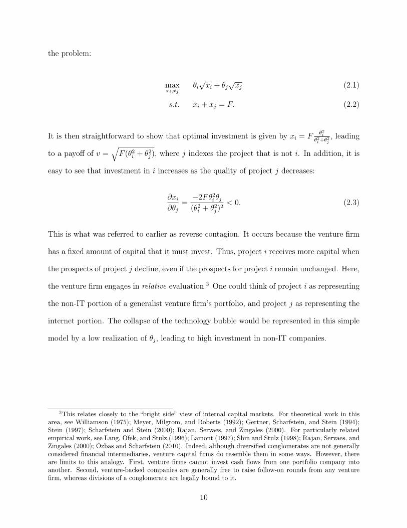
the problem:

max

xi,xj

✓

i

px

i

+ ✓

j

px

j

(2.1)

s.t. x

i

+ x

j

= F. (2.2)

It is then straightforward to show that optimal investment is given by x

i

= F

✓

2i

✓

2i+✓

2j, leading

to a payoff of v =

qF (✓

2i

+ ✓

2j

), where j indexes the project that is not i. In addition, it is

easy to see that investment in i increases as the quality of project j decreases:

@x

i

@✓

j

=

�2F✓

2i

✓

j

(✓

2i

+ ✓

2j

)

2< 0. (2.3)

This is what was referred to earlier as reverse contagion. It occurs because the venture firm

has a fixed amount of capital that it must invest. Thus, project i receives more capital when

the prospects of project j decline, even if the prospects for project i remain unchanged. Here,

the venture firm engages in relative evaluation.3 One could think of project i as representing

the non-IT portion of a generalist venture firm’s portfolio, and project j as representing the

internet portion. The collapse of the technology bubble would be represented in this simple

model by a low realization of ✓j

, leading to high investment in non-IT companies.

3This relates closely to the “bright side” view of internal capital markets. For theoretical work in thisarea, see Williamson (1975); Meyer, Milgrom, and Roberts (1992); Gertner, Scharfstein, and Stein (1994);Stein (1997); Scharfstein and Stein (2000); Rajan, Servaes, and Zingales (2000). For particularly relatedempirical work, see Lang, Ofek, and Stulz (1996); Lamont (1997); Shin and Stulz (1998); Rajan, Servaes, andZingales (2000); Ozbas and Scharfstein (2010). Indeed, although diversified conglomerates are not generallyconsidered financial intermediaries, venture capital firms do resemble them in some ways. However, thereare limits to this analogy. First, venture firms cannot invest cash flows from one portfolio company intoanother. Second, venture-backed companies are generally free to raise follow-on rounds from any venturefirm, whereas divisions of a conglomerate are legally bound to it.

10

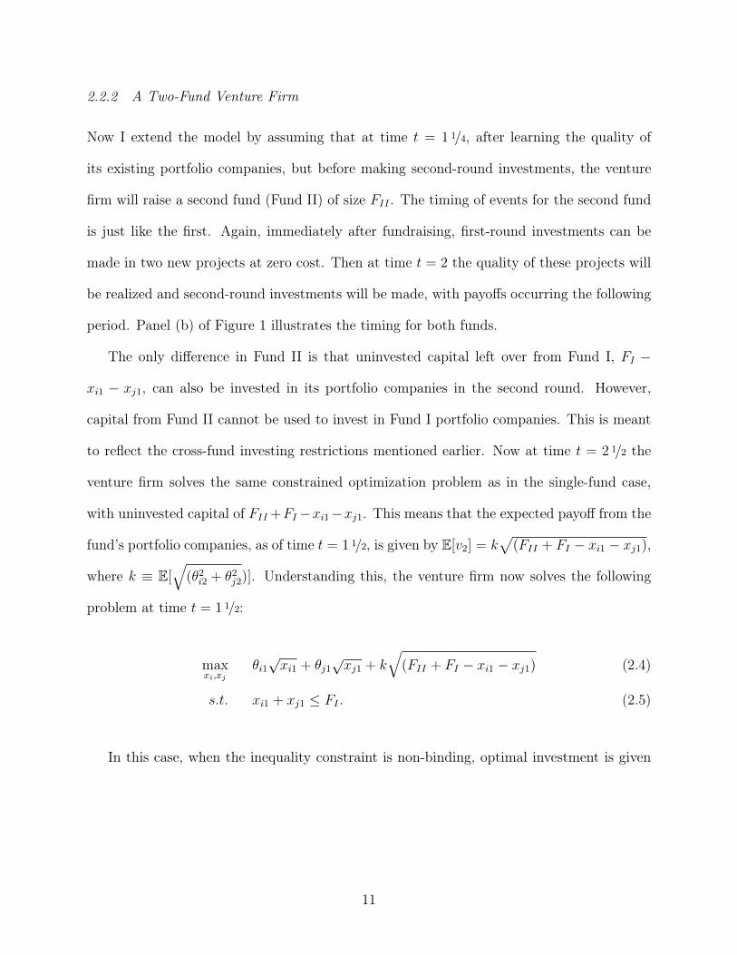
2.2.2 A Two-Fund Venture Firm

Now I extend the model by assuming that at time t = 1

1/4, after learning the quality of

its existing portfolio companies, but before making second-round investments, the venture

firm will raise a second fund (Fund II) of size F

II

. The timing of events for the second fund

is just like the first. Again, immediately after fundraising, first-round investments can be

made in two new projects at zero cost. Then at time t = 2 the quality of these projects will

be realized and second-round investments will be made, with payoffs occurring the following

period. Panel (b) of Figure 1 illustrates the timing for both funds.

The only difference in Fund II is that uninvested capital left over from Fund I, FI

�

x

i1 � x

j1, can also be invested in its portfolio companies in the second round. However,

capital from Fund II cannot be used to invest in Fund I portfolio companies. This is meant

to reflect the cross-fund investing restrictions mentioned earlier. Now at time t = 2

1/2 the

venture firm solves the same constrained optimization problem as in the single-fund case,

with uninvested capital of FII

+F

I

�x

i1�x

j1. This means that the expected payoff from the

fund’s portfolio companies, as of time t = 1

1/2, is given by E[v2] = k

p(F

II

+ F

I

� x

i1 � x

j1),

where k ⌘ E[q

(✓

2i2 + ✓

2j2)]. Understanding this, the venture firm now solves the following

problem at time t = 1

1/2:

max

xi,xj

✓

i1px

i1 + ✓

j1px

j1 + k

q(F

II

+ F

I

� x

i1 � x

j1) (2.4)

s.t. x

i1 + x

j1 F

I

. (2.5)

In this case, when the inequality constraint is non-binding, optimal investment is given

11

by:

x

i1 =

(F

II

+ F

I

)✓

2i1

k

2+ ✓

2i1 + ✓

2j1

(2.6)

) @x

i1

@✓

j1=

�2(F

II

+ F

I

)✓

2i1✓j1

(k

2+ ✓

2i1 + ✓

2j1)

2< 0. (2.7)

When the inequality constraint is binding, optimal investment is the same as in the

one-fund case.

Proposition 1. In the two-fund case without performance-sensitive fundraising, reverse

contagion ( @xi1@✓j1

< 0) still occurs in the region of the parameter space in which the inequality

constraint is non-binding; however, it is mitigated (the magnitude of @xi1@✓j1

is lower than in

the one-fund case).

Proof. See Appendix A.

The intuition behind this proposition is straightforward, as the capital that is not invested

in project j can now be saved for next period rather than needing to be invested immediately

in project i. Thus, future fundraising/investing can dampen the degree of reverse contagion.

2.2.3 A Two-Fund Venture Firm with Performance-Sensitive Fundraising

Now I allow F

II

to be a function of the average quality of projects realized in period 1:

F

II

= b(

✓i1+✓j1

2 ). This is a reduced form way of capturing the idea that limited partners will

be more reluctant to invest in a follow-on fund if the previous fund appears to have poor

interim performance (Kaplan and Schoar, 2005). This could be incorporated into a richer

model by allowing limited partners to learn about the talent of general partners through

interim performance. The parameter, b, above, captures the flow-to-performance sensitivity

of a venture firm. In this case, when the inequality constraint is non-binding, optimal

12

investment at time 1 will be given by:

x

i1 =

(b(

✓i1+✓j1

2 ) + F

I

)✓

2i1

k

2+ ✓

2i1 + ✓

2j1

(2.8)

) @x

i1

@✓

j1=

✓

2i

(b(k

2+ ✓

2i

� 2✓

i

✓

j

� ✓

2j

)� 4F

I

✓

j

)

2(k

2+ ✓

2i1 + ✓

2j1)

2. (2.9)

Proposition 2. In the two-fund case with performance-sensitive fundraising, there exists b

⇤

such that for b > b

⇤ ordinary contagion occurs ( @xi1@✓j1

> 0) in the region of the parameter

space in which the inequality constraint is non-binding.

Proof. See Appendix A.

Thus, for a venture firm whose fundraising is sufficiently sensitive to performance, in-

vestment in project i can now decline with the realized quality of project j. The reason

is that the decreased quality of project j leads to a smaller second fund. This decline in

total resources creates a force for decreased investment in both existing projects, which can

outweigh the increased relative attractiveness of project i with respect to project j. This is

true even despite the assumed cross-fund investing restrictions. Moreover, while the cross-

fund investing restrictions in the model allow Fund I to invest in the second-round of Fund

II projects, even this is not critical. For example, one could think of the second-round in-

vestments at time t = 2

1/2 as first-round investments and all of the results would remain

unchanged. Intuitively, what is important is that some of the capital that would have gone

into new projects from the new fund will now come from the old fund. Indeed, as long as

funds overlap temporally, there will always be semi-fungibility across funds, regardless of

restrictions.

13

2.3 Lock-in

While venture firms with high exposure to a depressed sector may indeed reduce the supply

of capital to unrelated clients, it does not necessarily follow that companies affiliated with

these investors should be harmed. If such companies were able to switch costlessly to another

venture firm, they would be unaffected by the poor performance of others originally held in

the same portfolio. However, there are several reasons why it may be difficult/costly to switch

venture firms or more generally to raise a new round of financing without the participation

of investors from the previous round.

Previous investors in a company accumulate a large amount of private information. This

is likely to be especially true in the context of venture capital, as venture investors are

known to be deeply involved in the operations of their portfolio companies4. Given this,

competing venture firms face a form of the winner’s curse in bidding against a better-informed

incumbent, making it difficult for portfolio companies to switch capital providers, much as

in Sharpe (1990) and Rajan (1992). Of course, if it were known that an incumbent ceased

investing in one of its portfolio companies due to unrelated financial difficulties, the winner’s

curse would no longer be in operation. It is not clear, however, that competitors are fully

aware of the details of one another’s financial health, especially as venture firms do not fail

abruptly, due to the long-term nature of limited partner commitments. To the extent that

a venture firm that is perceived to be in trouble continues investing in some companies but

not others, there will still be a winner’s curse.

Finally, even absent the winner’s curse, it remains true that much valuable information is

likely destroyed when relationships between venture firms and portfolio companies dissolve.

For example, suppose a company were known by its founders and original investors to be

4See e.g. Lerner (1995); Hellmann and Puri (2000, 2002); Baker and Gompers (2003); Kaplan andStrömberg (2004)

14

of high quality, but its original investors could no longer continue to support it for reasons

known by all to be unrelated to the company itself. In this case, new investors would still have

to value the company as one of merely average quality. At such a valuation, the founders’

participation constraints may not be satisfied, or they may be so diluted that they would

not have proper incentives. While in this case the original investors would like to transmit

their knowledge to another venture firm, such communication would not be credible given

the soft nature of their information and their incentives as existing shareholders.

3 Empirical Strategy

To investigate contagion among portfolio companies in venture capital, I examine continua-

tion financing outcomes for venture-backed non-IT companies during the period surrounding

the collapse of the technology bubble. In particular, I exploit variation in the degree of ven-

ture firms’ exposure to the internet sector. Again, this variation exists largely due to the

fact that some firms specialize in non-IT investments, while others make both IT and non-

IT investments. I will sometimes refer to generalist firms with high internet exposure as

“internet-focused venture firms.” However, note that the most internet-focused firms, many

of which became somewhat infamous in the wake of the bubble, will not be included in the

analysis. This is because I consider only firms that made at least some non-IT investments.

The most basic specification can be thought of as analogous to a difference-in-differences

estimation framework. Here, the treatment effect of interest is that of being held in the

same portfolio as many internet companies. A company is, thus, considered to be in the

treatment group if its investors had high internet exposure at the peak of the bubble and in

the control group if they had low exposure. The pre- and post- periods are defined as the

three years preceding and following the peak, respectively. The outcome of interest is the

15

likelihood of a portfolio company receiving a follow-on round of financing. One approach

would be to estimate a discrete response model with a dependent variable equaling one if

a company, i, considered for continued financing at time t received a follow-on round. The

difficulty with this approach is that, for companies that did not receive a follow-on round,

the time t at which they were considered and rejected is unknown. Furthermore, regardless

of whether the company was ultimately accepted or rejected for continued financing, it is

somewhat unrealistic to think of deliberation over this decision as having taken place at one

particular date.

To address these challenges, I instead estimate Cox proportional hazards models of the

form,

h

ijt

(⌧) = h0(⌧) exp(�1Post

t

+ �2InternetV C

ij

+ �3Post

t

⇥ InternetV C

ij

+ x

ijt

�), (3.1)

where i indexes portfolio companies, j indexes rounds of financing, and t indexes calendar

time. The variable ⌧ represents analysis time, which is defined as the time since company

i raised its previous round. The variables InternetV C

ij

and Post

t

are the treatment and

post indicators, respectively, while xijt represents a vector of controls. Using the language

of survival analysis, a spell is defined at the company-round level, and an event is defined as

the raising of a follow-on round. The outcome being modeled, hijt

(⌧), is continuation hazard

as a function of analysis time, conditional on covariates. To be more precise, the hazard

function is defined as the limiting probability that an event occurs in a given time interval

(conditional upon its not having occurred yet at the beginning of that interval) divided by

the width of the interval:

h(⌧) = lim

4⌧!0

Pr(⌧ +�⌧ > T > ⌧ |T > ⌧)

�⌧

, (3.2)

16

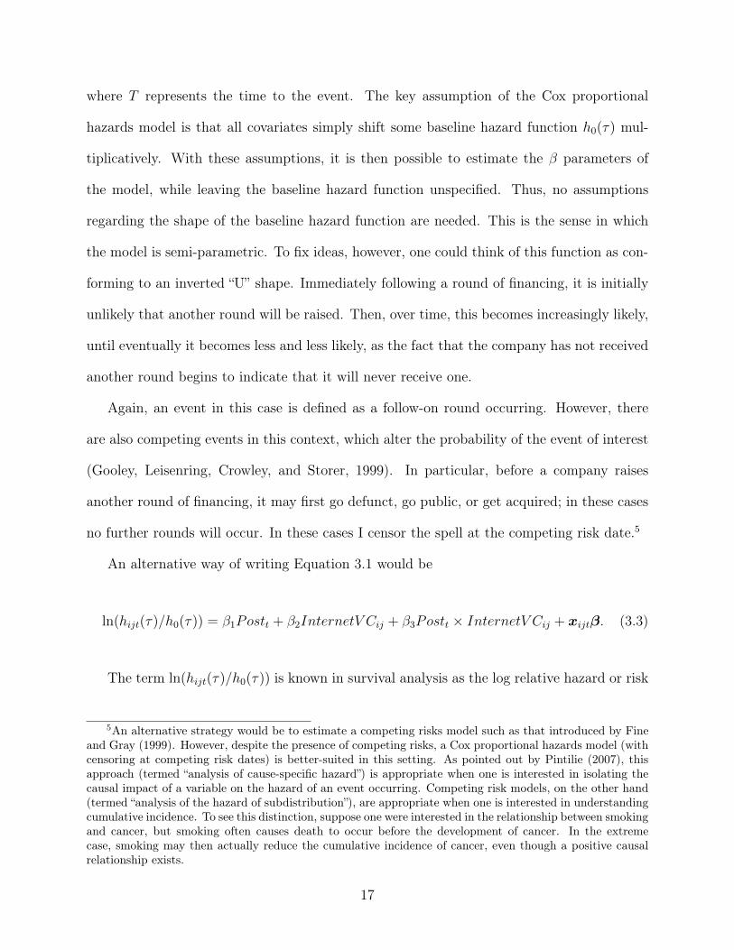
where T represents the time to the event. The key assumption of the Cox proportional

hazards model is that all covariates simply shift some baseline hazard function h0(⌧) mul-

tiplicatively. With these assumptions, it is then possible to estimate the � parameters of

the model, while leaving the baseline hazard function unspecified. Thus, no assumptions

regarding the shape of the baseline hazard function are needed. This is the sense in which

the model is semi-parametric. To fix ideas, however, one could think of this function as con-

forming to an inverted “U” shape. Immediately following a round of financing, it is initially

unlikely that another round will be raised. Then, over time, this becomes increasingly likely,

until eventually it becomes less and less likely, as the fact that the company has not received

another round begins to indicate that it will never receive one.

Again, an event in this case is defined as a follow-on round occurring. However, there

are also competing events in this context, which alter the probability of the event of interest

(Gooley, Leisenring, Crowley, and Storer, 1999). In particular, before a company raises

another round of financing, it may first go defunct, go public, or get acquired; in these cases

no further rounds will occur. In these cases I censor the spell at the competing risk date.5

An alternative way of writing Equation 3.1 would be

ln(h

ijt

(⌧)/h0(⌧)) = �1Post

t

+ �2InternetV C

ij

+ �3Post

t

⇥ InternetV C

ij

+ x

ijt

�. (3.3)

The term ln(h

ijt

(⌧)/h0(⌧)) is known in survival analysis as the log relative hazard or risk

5An alternative strategy would be to estimate a competing risks model such as that introduced by Fineand Gray (1999). However, despite the presence of competing risks, a Cox proportional hazards model (withcensoring at competing risk dates) is better-suited in this setting. As pointed out by Pintilie (2007), thisapproach (termed “analysis of cause-specific hazard”) is appropriate when one is interested in isolating thecausal impact of a variable on the hazard of an event occurring. Competing risk models, on the other hand(termed “analysis of the hazard of subdistribution”), are appropriate when one is interested in understandingcumulative incidence. To see this distinction, suppose one were interested in the relationship between smokingand cancer, but smoking often causes death to occur before the development of cancer. In the extremecase, smoking may then actually reduce the cumulative incidence of cancer, even though a positive causalrelationship exists.

17

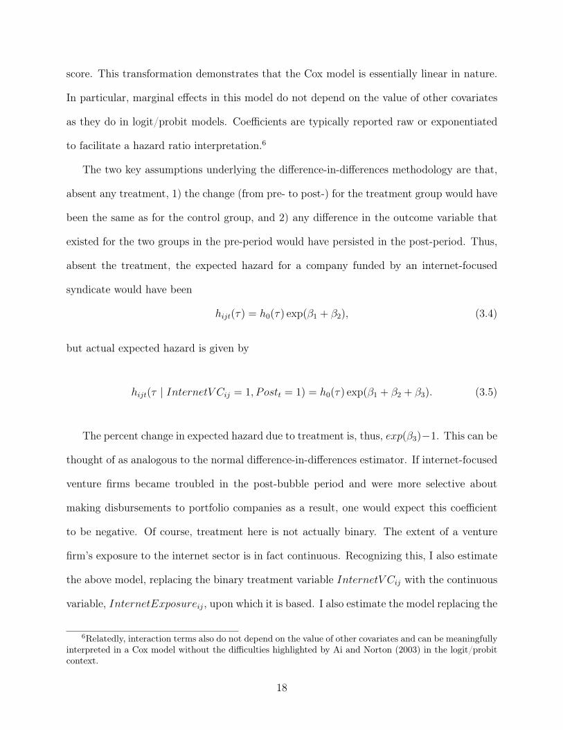
score. This transformation demonstrates that the Cox model is essentially linear in nature.

In particular, marginal effects in this model do not depend on the value of other covariates

as they do in logit/probit models. Coefficients are typically reported raw or exponentiated

to facilitate a hazard ratio interpretation.6

The two key assumptions underlying the difference-in-differences methodology are that,

absent any treatment, 1) the change (from pre- to post-) for the treatment group would have

been the same as for the control group, and 2) any difference in the outcome variable that

existed for the two groups in the pre-period would have persisted in the post-period. Thus,

absent the treatment, the expected hazard for a company funded by an internet-focused

syndicate would have been

h

ijt

(⌧) = h0(⌧) exp(�1 + �2), (3.4)

but actual expected hazard is given by

h

ijt

(⌧ | InternetV C

ij

= 1, Post

t

= 1) = h0(⌧) exp(�1 + �2 + �3). (3.5)

The percent change in expected hazard due to treatment is, thus, exp(�3)�1. This can be

thought of as analogous to the normal difference-in-differences estimator. If internet-focused

venture firms became troubled in the post-bubble period and were more selective about

making disbursements to portfolio companies as a result, one would expect this coefficient

to be negative. Of course, treatment here is not actually binary. The extent of a venture

firm’s exposure to the internet sector is in fact continuous. Recognizing this, I also estimate

the above model, replacing the binary treatment variable InternetV C

ij

with the continuous

variable, InternetExposure

ij

, upon which it is based. I also estimate the model replacing the

6Relatedly, interaction terms also do not depend on the value of other covariates and can be meaningfullyinterpreted in a Cox model without the difficulties highlighted by Ai and Norton (2003) in the logit/probitcontext.

18

binary variable Post

t

with the continuous variable log(InternetF lows

t

), which represents

aggregate flows to internet funds during the quarter corresponding to time t. The details

concerning the construction of these variables will be discussed in greater detail in the next

section.

The primary concern with the identification strategy outlined thus far is the potential

endogeneity of InternetExposure

ij

. Companies financed by venture firms with high internet

exposure might also have experienced a decline in their prospects coinciding with the collapse

of the technology bubble. Clearly, this would be the case if internet-focused venture firms

also tended to invest in portfolio companies in related IT sectors such as computer software

or communications, which is likely.

I address these endogeneity concerns in several ways. First, as previously described, I

restrict the sample to include only non-IT portfolio companies. These companies largely

operate in sectors such as biotechnology and energy, which have little direct connection with

the types of technologies that were driving the technology bubble. Thus, limiting the sample

to non-IT companies largely eliminates the possibility that the magnitude of the estimated

�3 coefficient is biased by the omission of a variable representing something akin to internet-

relatedness, with which InternetExposure

ij

might be positively correlated. Instead, the

concern would be that the prospects of non-IT companies that were backed by venture

firms with high internet exposure tended to decline in the post-bubble period due to other

omitted/unobservable characteristics.

Perhaps the most obvious potential candidate for such a characteristic is geography.

For example, if venture firms with high internet exposure tended to be located in Silicon

Valley and invested in portfolio companies near their headquarters, it may be that their non-

IT portfolio companies suffered a greater decline due to the decline in the local economy.

To account for this possibility, I include fixed effects for 13 regions (including Northern

19

California), as well as interactions between these fixed effects and the Post

t

indicator variable,

to control for the fact that companies in different regions might have felt differential effects

of the collapse of the technology bubble. Similarly, I include a full set of fixed effects for the

sector and stage of development of the portfolio company, as well as interactions between

those fixed effects and the Post

t

indicator. While this would seem to cover the most obvious

potentially omitted variables, it is of course still possible that non-IT companies backed

by internet-focused venture firms differed along some unobservable dimension that would

account for their greater decline in the post-bubble period.

To address this remaining possibility, I exploit the fact that companies can have relation-

ships with multiple venture firms. This allows me to run related tests that include company

fixed effects. Identification in this case is based on within-company variation in investor

internet exposure. Thus, I am able to examine whether the same company was less likely to

receive continuation financing from those of its investors that had greater exposure to the

internet sector. Such a result could not be explained by unobservable company characteris-

tics. Rather, it would suggest a decrease in the supply of capital from investors with high

internet exposure.

4 Data

The data used in this study come from the Thomson-Reuters VentureXpert database. These

data contain information on both venture capital financing rounds (including the round date,

the identities of the venture firms and portfolio company participating, and the size of each

venture firm’s contribution to the round), and venture firm fundraising (including the size

and closing date of all funds raised by a firm). I restrict the sample to venture capital

financing rounds involving U.S. portfolio companies. In addition, only companies that are

20

categorized by Thomson as non-IT are included. Finally, I also include only rounds that

were backed by venture capital organizations structured as autonomous partnerships. Thus,

rounds backed entirely by individuals, or entities such as corporate-sponsored venture funds,

are omitted.

The estimation window runs from March 31, 1997, to March 31, 2003. Some spells begin

before the estimation window, but end during the estimation window. Likewise, some spells

begin during the estimation window, but end after the window. These spells are censored

appropriately at the boundaries. In addition, as mentioned earlier, spells are also censored

at competing risk event dates (when a company goes defunct, goes public, or gets acquired).

In some cases, particularly for companies that ultimately went defunct, the date of the

competing risk event is unknown. In these cases, I censor the spells at two years after the

last observed financing round. The results are not sensitive to this assumption.

Another issue with the data, previously reported by Lerner (1995), is that some com-

panies appear to have too many financing rounds recorded. This is likely due to staggered

disbursements from a single round being misrecorded as multiple rounds. Also, a small num-

ber of companies have consecutive rounds that are extremely far apart. I, thus, restrict the

sample to companies with rounds no less than 30 days and no more than six years apart.

Again, the results change little if these companies are included.

4.1 Key Measures

4.1.1 Dating the Peak

The post-bubble period, in which the Post

t

indicator variable is set equal to one, is de-

fined as all dates following March 31, 2000. This is motivated by Figure 2, which shows

the buy-and-hold return on publicly traded internet stocks. Internet stock returns are cal-

culated as in Brunnermeier and Nagel (2004) and Greenwood and Nagel (2009), using a

21

value-weighted portfolio of stocks in the highest NASDAQ price/sales quintile, rebalanced

monthly.7 Quarterly flows to newly raised venture funds are also shown, both for all funds

and internet-specific funds, as categorized by Thompson-Reuters.8 Commitments are con-

verted to real 2000 dollars using the GDP deflator. The dotted vertical line in the figure

corresponds to March 31, 2000, which is the peak of all three series. Thus, not only did

internet stocks peak at this date, but so did venture capital fundraising. The estimation

window is chosen accordingly to run from three years prior to the peak (the pre-period) to

three years following the peak (the post-period).

4.1.2 Measuring Internet Exposure

The degree of a venture capital firm k’s exposure to internet investments, InternetExposure

k

,

is measured as the percentage of the total amount invested by the firm that was disbursed

to companies operating in the internet sector during the 10 years leading up to the peak. A

10-year window is chosen as this is the life of a typical venture fund, although results are

similar if a shorter window is used. To limit the effect of outliers that may occur due to firms

with few investments in the data, firms with less than five observed investments during this

period are considered to have unknown internet exposure.9

7As Greenwood and Nagel explain, this methodology is used because SIC codes fail to identify the bubblesegment of the market in many cases. For example, the internet stock eBay has SIC code 738, which placesit in the Business Services industry.

8Note that internet-specific fund flows do not fully reflect the amount of money raised by venture capitalfirms for internet investments, as many funds made substantial internet investments, but were not categorizedas internet-specific funds.

9Note that this measure of internet exposure includes investments in companies that went public, wereacquired, or went defunct prior to the peak. An alternative approach would be to look only at a firm’sactive portfolio as of March 31, 2000, to determine its internet exposure. Trying to isolate active portfoliocompanies at the peak, however, is somewhat complicated again by the fact that the date of failure fordefunct companies is usually unknown. Another complication is that lockup provisions typically restrictventure firms from selling their shares for some period of time following an IPO. In any case, it is not clearthat this is conceptually the measure of interest, as even if a venture firm did not hold many active internetcompanies in its portfolio at the peak of the bubble, if it were perceived as an internet specialist due toits investment history, it would likely have faced difficulty raising a new fund in the post-bubble periodregardless.

22

Funding rounds are often financed by syndicates of multiple venture firms. In this case

internet exposure is defined at the syndicate level. Specifically, for the syndicate backing the

jth round of company i, internet exposure is defined as 1) the mean of InternetExposure

k

for

all venture firms participating in the round, weighted by their contribution to the round and

2) the value of InternetExposure

k

for the lead investor in the round. For the first measure,

internet exposure is weighted by firm contribution rather than firm assets under management

because a portfolio company would likely be most adversely affected if its primary investor

were in trouble, even if that investor were not the largest in the syndicate based on assets

under management. For the second measure, the lead venture firm is taken to be the one

that has invested in the company the longest, as in Gompers (1996). Ties are broken by the

total amount invested in the company, inclusive of the current round. Using this definition,

a lead venture firm cannot be uniquely identified in some cases and is then simply considered

to be unknown.

4.1.3 Non-IT Classification

Finally, one potential concern with these data is that companies may be classified as non-IT,

when in fact they make use of technologies related to the bubble. For example, one may

worry that a company like WebMD, a website that provides health information for patients,

may be considered to be in the health sector and therefore categorized as a non-IT company.

Importantly, Thomson does not make the IT/non-IT distinction based on sub-sector; rather,

this depends on a company’s use of technology. Thus, not all health-related companies are

considered non-IT. In particular, Thomson provides six sector classification variables that

range from very coarse (3 categories) to very detailed (570 categories). According to these

variables, WebMD is classified as 1) “Information Technology,” 2) “Computer Related,” 3)

“Internet Specific,” 4) “Internet Specific,” 5) “Internet Content,” and 6) “Medical/Health

23

Info/Content.” In contrast, there are other “Medical/Health Info/Content” companies in the

data that are classified as non-IT. The high level of detail contained in these classifications,

as well as the fact that the IT/non-IT distinction is not based solely on sub-sector variables,

gives some comfort that the non-IT classifications are at least largely correct. In addition,

Thomson provides detailed business descriptions, product key words, and technology class

descriptions. Results are robust to excluding companies that might be considered more

likely to be IT-related based on these variables. In addition, when company fixed-effects are

included, they control for unobservable IT-relatedness.

4.2 Summary Statistics

After the sample restrictions described above are imposed, I am left with observations on

782 venture firms, funding 6,104 rounds of 3,263 companies. Table 1 shows the composition

of the sample both in terms of companies and rounds.10 Rounds are the relevant unit of

observation in most of the analysis to follow in the next section. Panel (a) breaks down

the sample by region. As speculated earlier, rounds backed by venture firms in the top

quartile of internet exposure (InternetV C

ij

= 1) are much more likely to be associated

with portfolio companies located in Northern California than rounds in the bottom quartile

(InternetV C

ij

= 0). The differences in the regional distributions are confirmed by a chi-

square test. Panel (b) shows the breakdown of companies by sector. Life sciences companies

operating in the medical/health and biotechnology sectors account for more than half of the

observed financing rounds.

Finally, Panel (c) breaks the sample down by stage. In this case, only the round level

is shown, as companies change stages from round to round. The order of the stages from

least developed to most are startup/seed, early, expansion, and later. By far, the most

10These differ as the average company in the sample received nearly two rounds of financing.

24

common stage financed is the expansion stage with slightly more than 50% of observed

rounds occurring at this stage.

Summary statistics of the key variables used in the analysis are presented in Table 2.

These statistics are presented at varying units of observation as appropriate. For example,

the internet exposure of syndicates backing rounds is shown at the round level. As described

earlier, this is measured for the whole syndicate as well as the lead venture firm in the

syndicate.11 Both measures of internet exposure appear to be distributed similarly with a

mean of nearly 19%. Thus, the average round in the sample was backed by venture firms that

made 19% of their total disbursements to internet companies in the decade leading up to the

peak of the bubble. The mean number of investors in a round was slightly less than three.

The distribution of internet exposure is also shown at the venture firm level. The average

venture firm had internet exposure of 24%, indicating that lower exposure companies must

have funded more rounds in the data. Though not shown in the table, the modal internet

exposure in this sample of firms making non-IT investments was zero, with slightly more

than 20% of firms having no internet investments at all. As stated earlier, internet exposure

is based on observed investments in the 10 years leading up to the peak. The average firm

in the sample had almost 60 observed investments during this period.

5 Results

5.1 On Average, IT Companies Affected, Non-IT Companies Unaffected

I begin by verifying that IT companies, and particularly internet companies, had greater

difficulty raising continuation financing in the post-bubble period. Were this not the case, it

11When the lead venture firm cannot be uniquely identified, the former may be known while the latter isnot. When the round contributions of firms in the syndicate are not recorded in the data, the reverse maybe true.

25

would seem unlikely that non-IT companies backed by more internet-focused investors would

have experienced negative effects from the collapse of the bubble. I estimate univariate Cox

models of the form

h

ijt

(⌧) = h0(⌧) exp(�1Post

t

) (5.1)

for each IT sector in the data. Results are shown in Panel (a) of Table 3. Standard errors

are clustered by portfolio company. The implied percent change in hazard from before to

after the peak, exp(�1) � 1, is shown below the raw coefficients. For companies in most

of the IT sectors, the hazard of raising a continuation round was considerably lower in the

post-bubble period. In particular, companies in the communications, hardware, and software

sectors experienced a decrease in hazard of more than 20%. As expected, companies in the

internet sector were hit the hardest. Internet companies are estimated (with high precision)

to have had a decrease in hazard of more than 50%.

The results for non-IT sectors are shown in Panel (b). Companies in non-IT sectors

did not, on average, suffer major declines. At conventional level of significance, biotech,

consumer, energy, medical, and other non-IT companies all had a statistically insignificant

change in hazard in the post-bubble period. Moreover, noisy point estimates indicate a

less than 10% decline in all non-IT sectors except energy, which is estimated to have had

nearly a 9% increase. While interesting to note, this is not necessary for my identification

strategy to be valid, as I will be comparing the experience of non-IT companies backed by

investors with high and low internet exposure. Put differently, the difference-in-differences

methodology does not require that the control group be unchanged in the post-period.

26

5.2 Non-IT Companies Backed By Internet VCs Were Affected

5.2.1 Difference-in-Differences, Extreme Quartiles

Next, I limit the sample to non-IT companies and estimate the difference-in-differences spec-

ification of Equation 3.1. The treatment indicator variable, InternetV C

ij

, is set equal to one

if InternetExposure

ij

(for the venture firms backing the jth round of company i) is in the

top quartile of all rounds. The treatment indicator is set equal to zero if InternetExposure

ij

is in the bottom quartile. Rounds in the middle two quartiles are omitted under this speci-

fication because it is difficult to discretely categorize rounds with InternetExposure

ij

near

the median as either treated or untreated. Referring to the summary statistics presented in

Table 2, the 25th percentile of InternetExposure

ij

is between 5% and 7%, depending on

how the exposure of a syndicate is measured; the 75th percentile is around 27%.

Table 4a reports the results. Standard errors are clustered by portfolio company in the

first three columns as well as by lead firm in the last three columns (Cameron, Gelbach, and

Miller, 2011). The estimated percent change in hazard due to treatment, exp(�3)�1, is shown

below the raw coefficients. Beginning with Column (1), the estimate of �3 is negative and

statistically significant. The magnitude of the coefficient implies a decline in continuation

hazard of 31% due to treatment. Thus, the estimated effect is quite substantial. The coef-

ficient on InternetV C

ij

is also positive and statistically significant under this specification.

This suggests that, relative to other non-IT companies, those backed by internet-focused syn-

dicates had less difficulty raising follow-on rounds before the collapse. This will be explored

in more depth, but turns out not to be as robust as the main finding.

Again, with the proportional hazards assumption, the baseline hazard function is left

unspecified. However, given the estimated � coefficients, a smoothed estimate of the implied

baseline hazard function can be backed out. It is useful to examine the shape of this function

27

to ensure that it is reasonable. Figure 3 shows the hazard functions derived from Column (1)

of Table 4a. The proportional shifts in the baseline hazard, shown at various values of the

covariates, simply reflect the estimated coefficients just discussed. As speculated earlier, it

does appear that the baseline hazard function conforms to an inverted “U” shape. The figure

shows graphically that non-IT companies backed by internet-focused syndicates experienced

a decrease in continuation hazard in the post-bubble period (Panel a), whereas those backed

by non-internet syndicates experienced a statistically insignificant increase (Panel b). The

difference in these differences is the estimated treatment effect.

Another way of understanding the economic magnitudes implied by these estimates is to

examine the implied survivor function, S(⌧) = Pr(T > ⌧), which reports the probability of

an event not having occurred yet as of time ⌧ . In this case, a portfolio company would be

said to have “survived” until time ⌧ if it had not received continuation financing as of that

time. Intuitively, downward shifts in the hazard function correspond to upward shifts in

the survivor function. In fact, there is a one-to-one inverse relationship between cumulative

hazard and the survivor function.

Figure 4 shows how the survivor function shifted for the treatment and control groups,

again based on Column (1) of Table 4a. Examining the survivor function is useful, as it pro-

vides magnitudes that are perhaps more easily interpreted. For example, the estimates imply

that, after five years, the probability of not having yet raised a follow-on round increased

by 8.3% for the treatment group and decreased by 4.1% for the control group. As discussed

earlier, going too long without a follow-on round of financing typically leads venture-backed

companies to go defunct. Thus, in terms of real effects, these estimates likely imply that

companies in the treatment group had a significantly larger increase in their failure rate.12

12Ideally, this could be tested more directly. However, conducting such a test is difficult for two reasons.First, company failure dates are often unknown. Second, liquidations are often coded in the data as acquisi-tions rather than failures. Thus, it is difficult to assess both whether a company failed and, if it failed, whenthe failure occurred.

28

In Column (2) of Table 4a, company stage, region, and sector fixed effects are added

to the specification. In Column (3), I allow interactions between the company controls and

the Post

t

indicator. As previously discussed, this is important, as companies with certain

characteristics might have been both more adversely affected by the collapse of the bubble

and also more likely to have been funded by a more internet-focused syndicate. After adding

these controls, the estimated treatment effect remains large and statistically significant.

Moreover, the small change in the point estimates between Columns (2) and (3) suggests that

the results in the previous columns were not driven by a tendency for more internet-focused

firms to have invested in non-IT companies with observable characteristics that made them

worse investments after the bubble. It remains possible that unobservable characteristics of

this kind are driving the results. This will be addressed shortly. In Columns (4) through

(6), I estimate the same specifications as in the first three columns, but define the variable

InternetV C

ij

based on the internet exposure of only the lead venture firm in the round.

This gives rise to similar results.

Next, I estimate the same regressions, substituting the continuous variable InternetExposure

ij

for InternetV C

ij

and making use of the entire sample. This takes advantage of the fact

that treatment is not actually binary in this case. Results are reported in Table 4b and

are very similar to the previous panel. To interpret the magnitudes of these estimates,

note that the percent change in hazard associated with the end of the bubble is equal

to exp(�1 + �3InternetExposure

ij

) � 1. Substituting the coefficients from Column (1),

this expression evaluates to �15.8% for a portfolio company backed by venture firms with

mean internet exposure (of 24.4%). For a portfolio company backed by venture firms with

InternetExposure

ij

one standard deviation above the mean (47.9%), the collapse of the

bubble was associated with a �33.4% change, or a 17.6% larger decrease in hazard. In the

remaining specifications, this difference is similar, ranging from 14.3% to 17.2%. So again,

29

the magnitude of the estimated effect is substantial.

Finally, I also estimate these equations once more on the whole sample, substituting

the variable log(InternetF lows

t

) for Post

t

, where log(InternetF lows

t

) represents the log

of all flows to internet-specific venture capital funds raised in the quarter corresponding to

time t. Thus, instead of defining discrete pre- and post- periods, this specification takes

advantage of the continuous variation over time in the perceived prospects of young internet

companies, as reflected by flows into internet-specific funds. Results are reported in Table

4c, with standard errors now clustered also by quarter. Across all six specifications, there is

an estimated positive and statistically significant interaction between log(InternetF lows

t

)

and InternetExposure

ij

, providing evidence that non-IT companies backed by venture firms

with greater internet exposure were more sensitive to fluctuations in the internet sector. Note

that �1 is also statistically insignificant across all six specifications, which suggests that non-

IT companies backed by venture firms with no internet exposure were not sensitive at all to

these fluctuations.

5.2.2 Additional Robustness Tests

One concern at this point is that some of the companies classified by Thomson as non-

IT may in fact have been IT-related. If this were the case, it might simply add noise to

the results, without introducing any systematic bias. However, bias would be introduced

if non-IT portfolio companies backed by venture firms with internet investments tended to

be miscatergorized as non-IT more frequently. Another related concern is that, even if no

companies were misclassified, those backed by more internet-focused investors may have had

other unobservable characteristics that caused their prospects to decline when the bubble

burst. Both of these possibilities will be addressed shortly by examining portfolio companies

with multiple investors and including company fixed effects. The miscategorization problem

30

can also be examined, however, by repeating the above analysis on sub-samples that are less

likely to include IT-related companies. This is done in Table 5. Column (1) of this table

replicates Column (6) of Table 4b, excluding all non-IT companies classified by Thomson

as “Consumer Related.” Similarly, Column (2) excludes all non-IT companies producing

“Other Products.” Column (3) excludes all non-IT companies with variations of the words

“Internet,” “Online,” “Web,” “E-Commerce,” “Software,” “Digital,” “Electronic,” “Computer,”

“E-mail,” “Hardware,” or “Network” in their detailed business description, product keywords,

or technology description. In Column (4), companies that are categorized as IT by Dow

Jones’ VentureSource database are excluded.13 In all four sub-samples, the coefficient on

Post

t

⇥ InternetExposure

ij

continues to be negative and statistically significant. Thus the

effect continues to be strongly present, even in sub-samples that are less likely to contain

IT-related companies.

5.3 Continuation Hazard Did Not Increase as Bubble Inflated, Decreased as

Deflated

The results thus far suggest that the decline in a company’s continuation hazard when the

bubble burst was greater the greater the internet exposure of its investors. It is not clear,

however, whether this greater decline in continuation hazard primarily reflected hazard being

“too high” during the bubble period or “too low” during the post-bubble period. Put another

way, contagion among portfolio companies may have taken place both on the upside as well

as on the downside. In general, it is not possible to distinguish between these two scenarios

using a difference-in-differences framework. It is possible, however, to shed some light on

this issue using the quarterly flows specification. In particular, if contagion occurred on the

upside, one would expect continuation hazard to have increased along with InternetF lows

t

13VentureSource is another major venture capital database. Portfolio companies are matched using acombination of name, address, phone number, and URL.

31

as the bubble inflated. To test whether this occurred, I re-estimate the specifications of

Table 4c, now allowing the interaction between internet flows and venture firm internet

exposure to differ before and after the peak of the bubble. Results are reported in Table 6.

In all specifications, the estimated interaction in the pre-period is statistically insignificant.

This suggests that, as the bubble inflated, non-IT portfolio companies did not become more

likely to receive follow-on rounds, even if their venture firm was heavily invested in the

internet sector. By contrast, the estimated interaction in the post-period is positive and

statistically significant across all specifications. This suggests that, as the bubble deflated,

portfolio companies did become less likely to receive follow-on rounds, particularly if their

venture firm was heavily invested in the internet sector. On the whole, these results provide

evidence that contagion among portfolio companies primarily occurred on the downside.

5.4 For Same Company, Internet VCs Became More Likely to Drop Out of

Rounds

It still remains possible that non-IT companies backed by more internet-focused venture firms

differed from others along some unobservable dimension that made them worse investments

in the post-bubble period. In this case, these companies may have had more difficulty

raising continuation financing, not because they were held in the same portfolio as internet

companies, but because their own future prospects deteriorated alongside those of internet

companies. To investigate whether the previous results are driven by unobservable company

characteristics of this kind, I run related tests that include company fixed effects. It is

possible to include these fixed effects because, as noted earlier, venture-backed companies

frequently take capital from multiple investors. Identification in this case is based on within-

company variation in investor internet exposure. Thus, I am able to examine whether the

same company was less likely to receive continuation financing from those of its investors

32

that had greater exposure to the internet sector. Such a result could not be explained by

demand-side factors, i.e. company characteristics. Rather, it would suggest a decrease in

the supply of capital from investors with internet-heavy portfolios.

To address these issues, I run related tests that do not make use of the proportional

hazards framework. Instead, I limit attention to rounds that were actually raised, and

estimate whether previous investors with high internet exposure were more likely to drop

out of these rounds after the bubble burst. This can be thought of as relating to the intensive

margin (i.e. conditional on raising a round, did investors continue to participate?), whereas

previous results related to the extensive margin (i.e. was a round raised from any investor?).

For each continuation round raised by a company, I form an observation for each venture

firm that participated in the previous round. If the venture firm participated in the current

round, V CDropout

ijkt

is equal to zero; otherwise, V CDropout

ijkt

is equal to one.14

I then estimate linear probability models of the form,

V CDropout

ijkt

= ↵

i

+ �1Post

t

+ �2InternetExposure

k

+ �3Post

t

⇥ InternetExposure

k

,

(5.2)

where ↵

i

represents a company fixed effect. Observations in this case are at the company-

round-VC level (k indexes VCs). The primary coefficient of interest is again �3. If estimated

to be positive, this would indicate that greater internet exposure was associated with a

greater increase—from before to after the peak of the bubble—in the probability of dropping

out of a round.

Table 7 reports the results. As InternetExposure

k

varies only at the venture firm level,

standard errors are clustered accordingly by venture firm as well as portfolio company. In

14One exception to this rule is made if the venture firm is observed participating again in subsequentrounds of the company. Then, the firm is considered a participant in the current round, as its omission istaken to be a data error.

33

the first two columns, Equation 5.2 is estimated via OLS without company fixed effects. In

the final two columns, company fixed effects are included. Across all specifications, �3 is

estimated to be positive and statistically significant, with point estimates decreasing only

slightly with the inclusion of company fixed effects. The coefficients in the final column

imply that a one standard deviation increase in internet exposure was associated with a

4.16% larger increase in the probability of dropping out of a round after the bubble burst.

Considering that the unconditional probability of a firm dropping out in the pre-period

was only 10.8%, these magnitudes are again economically meaningful, as they represent a

percentage increase of 38.5. This provides perhaps the clearest evidence that more internet-

focused venture firms ceased supporting companies that they would have liked to continue

to support.15

Finally, it should be said that these results do imply that some companies were able to

overcome lack of participation from previous investors. However, there is no inconsistency

between these findings and those presented previously. Indeed, if none were able to overcome

investor dropout, results would be found only on the extensive margin. Similarly, if all were

able to do so, results would be found only on the intensive margin.

5.5 Internet VCs Had Increased Fundraising Difficulty After Collapse

Next, I explore the mechanism underlying these results. As discussed earlier, the most obvi-

ous mechanism through which ordinary contagion might occur is through the transmission

of fundraising difficulties. It seems quite plausible that venture firms with internet-heavy

portfolios would have had trouble raising new funds from limited partners after the bubble

burst. To investigate this, I estimate the same hazard models as before, but now at the

15Note that �

2

, the coefficient on Post

t

, is estimated to be negative without company fixed effects andpositive with company fixed effects. This is likely due to selection, as companies that received follow-onrounds in the post-bubble period may have been of higher quality and thus experienced fewer investordropouts.

34

venture firm level. Specifically, rather than estimating the hazard of a portfolio company

raising a continuation round from venture firms, I now estimate the hazard of a venture firm

raising a follow-on fund from limited partners. In the three columns of Table 8, I repeat the

three specifications of Table 4 at the venture firm level. Standard errors are clustered by

venture firm and also by quarter in the third column.

The same general pattern emerges as at the portfolio company level. The coefficients

on the interaction terms Post

t

⇥ InternetV C

k

and Post

t

⇥ InternetExposure

k

are both

estimated to be negative, while the coefficient on log(InternetF lows

t

)⇥InternetExposure

k

is estimated to be positive; all are statistically significant. This suggests that the adverse

effect of the collapse of the technology bubble on fundraising was greater for venture firms

that were more associated with internet investing. The magnitudes of these estimates are

again substantial. For example, the coefficients in Column (1) imply that venture firms in

the top quartile of internet exposure had a 47.5% larger decrease in fundraising hazard than

those in the bottom quartile.

5.6 Companies Backed By Young VCs Late in Fundraising Cycle Were Most

Affected

Thus, internet-focused venture firms faced increased difficulty in raising new funds after the

collapse of the bubble. Also, at the same time, non-IT companies funded by these firms had

increased difficulty in obtaining continuation financing in the post-bubble period. While

these two facts would appear connected, little evidence has yet been presented to directly

establish such a connection. If portfolio companies associated with more internet-focused

venture firms were indeed less able to raise follow-on rounds due to the diminished fundraising

capacity of their investors, one would expect the negative effect of investor internet exposure

to be strongest for companies backed by firms that had not raised a new fund recently. This

35

follows because such venture firms would be more likely to be running low on uninvested

capital and, therefore, to be concerned about a decline in their fundraising capacity.

To test this, I re-estimate the specifications of Table 4b, now allowing all of the pri-

mary variables to interact with Y earsSinceRaised

ijt

, a variable representing the num-

ber of years since the venture firms backing the jth round of company i last raised a

fund. In addition to these interactions, I also include an additional set of controls for

Post

t

⇥ InternetExposure

ij

⇥ Stage

ij

and InternetExposure

ij

⇥ Stage

ij

to ensure that

terms involving Y earsSinceRaised

ijt

do not also pick up effects from the stage of develop-

ment of portfolio companies.16

Results are reported in Table 9. The primary coefficient of interest is that on the triple

interaction term Post

t

⇥ InternetExposure

ij

⇥ Y earsSinceRaised

ijt

, which is estimated to

be negative and statistically significant in Columns (3) through (6) and marginally significant

in Columns (1) and (2). Overall, this suggests that the negative effect of the bubble’s collapse

on portfolio companies backed by high internet exposure firms was greater the longer it had

been since those firms raised a new fund. Also, note that the estimated coefficient on the

double interaction Post

t

⇥ InternetExposure

ij

is not statistically significant. Therefore, it

is not possible to reject the null that, for a company backed by a venture firm with a newly

raised fund (Y earsSinceRaised

ijt

= 0), internet exposure was unrelated to the change in

continuation hazard.

A venture firm’s recent investment history would likely affect its fundraising less if the

firm had a long previous investment track record. This would occur, for example, if limited

partners updated their beliefs about a firm’s investment ability in a Bayesian manner.17

16This may occur, for example, if low Y earsSinceRaised

ijt

rounds tend to be in earlier-stage companies.17Consistent with this, many well-established firms, including Kleiner Perkins, Charles River Ventures,

and Accel Partners, returned capital to limited partners after the collapse, citing reduced investment oppor-tunities. Such behavior would certainly seem to indicate that these firms were confident in their ability toraise future funds. Young venture firms, on the other hand, were likely less confident.

36

Thus, if companies backed by young firms were more affected by the internet exposure of

their investors, this would provide further evidence that venture firm fundraising difficulties

were indeed driving the baseline results. Indeed, the model presented earlier predicts that

contagion should occur only if fundraising is sufficiently sensitive to performance, which

would more likely be true for young venture firms.

I therefore re-estimate the specifications of the previous table, now allowing all the pri-

mary variables to further interact with Y oungV C

ij

, an indicator variable equaling one if

the lead venture firm in the round was less than six years old at the peak of the bubble

and zero otherwise. For expositional clarity, I present the results for the Y oungV C

ij

= 1

and Y oungV C

ij

= 0 subgroups separately, so as to avoid showing quadruple interaction

terms.18 Results are presented in Table 10. The primary coefficient of interest is again that

on the triple interaction term Post

t

⇥ InternetExposure

ij

⇥ Y earsSinceRaised

ijt

. In the

first three columns, this coefficient is estimated to be negative and statistically significant

for the Y oungV C

ij

= 1 subgroup. In the final three columns, it is estimated to be smaller

in magnitude and statistically insignificant for the Y oungV C

ij

= 0 subgroup. Most im-

portantly, the difference in this coefficient for the two subgroups is large and statistically

significant across all specifications. Therefore, to summarize, the portfolio companies that

experienced the largest decline in continuation hazard when the technology bubble burst

were those backed by venture firms that 1) had high internet exposure, 2) had not raised a

fund recently, and 3) had a short previous investment track record. Again, these results are

consistent with the venture firm fundraising mechanism.

18Note, however, that the region/stage/sector controls are in fact estimated using the whole sample.

37

5.7 Companies Backed by Internet VCs Were No Less Productive Prior to

Collapse

Much of the discussion up to this point has implicitly assumed that non-IT companies

funded by internet-focused venture firms were similar in quality to other non-IT companies.

However, it is also possible that internet-focused venture firms tended to fund low-quality

non-IT companies during the bubble and cut back funding to these companies subsequently.

Note, the issue of quality is distinct from the endogeneity concerns discussed earlier. Again,

due to the difference-in-differences framework used, the primary challenge to identification

here comes not from unobservable differences in the level of company prospects, but rather

unobservable differences in changes in company prospects coinciding with the end of the

bubble. Thus, even if these companies tended to be of low quality, it might still be correct to

say that the decline of the internet sector, coupled with the high exposure of their investors

to that sector, caused them to lose access to capital. However, the welfare implications of

that statement would change if these companies were negative NPV.19 This might be the

case if internet-focused venture firms anticipated high returns on their internet holdings and

took chances on bad non-IT investments as a result. This would in some ways be akin to the

agency costs of free cash flows (Jensen, 1986). On the other hand, one could also argue that

the opposite might have been true. That is, venture firms with substantial internet holdings

might have been more selective about making non-IT investments during the bubble period,

as they might have perceived a larger opportunity cost in doing so.

To shed light on this issue, I examine whether companies with more internet-focused

investors were less productive in terms of their patenting activity before the collapse of the

19This again parallels the internal capital market literature. While Lamont (1997) and others establishthat diversified firms reallocate funds across divisions, it is not clear whether this is efficient. This questionis taken up separately by e.g. Scharfstein (1998), Rajan, Servaes, and Zingales (2000), Whited (2001), andChevalier (2004).

38

bubble. As discussed earlier, many of the companies in the sample operate in the biotech-

nology and medical/health sectors, where patents play a crucial role. I obtain patent data

from the National Bureau of Economic Research (NBER) Patent Data Project (Hall, Jaffe,

and Trajtenberg, 2001). These data are then matched with Thomson on company name,

using the name standardization and matching procedures developed by the NBER Patent

Data Project.20 Matches are confirmed manually. I then limit the sample to companies that

raised their first round of financing in the three years prior to the peak of the bubble (March

31, 1997, to March 31, 2000). For each company, I calculate the total number of successful

patents applied for before the collapse. Also, for each of these patents, I calculate the total

number of citations received during the three years following the date on which the patent

was granted. Citations are a well-established proxy for the economic importance of a patent

(Jaffe and Trajtenberg, 2002). As in Lerner, Sorensen, and Stromberg (2011), citations are

counted for only a three-year window so that earlier patents do not have greater time to

garner citations. Because both total patents and citations are count variables, I follow the

literature and estimate negative binomial models of the form,

�

i

= exp(�0 + �1InternetExposure

i

+ x

ijt

�), (5.3)

where �i

is the intensity parameter. When total patents are the outcome of interest, i indexes

portfolio companies; when citations are the outcome of interest, i indexes individual patents.

Results are reported in Table 11 with coefficients reported in terms of mean marginal ef-

fects to ease interpretation. In Columns (1) and (3), i indexes portfolio companies and �

i

rep-

resents company patenting intensity.21 In both columns, the coefficient on InternetExposure

i

20See https://sites.google.com/site/patentdataproject/Home for the name-standardization programs andmatching scripts used.

21In this analysis, companies differ in terms of their exposure time (the time they had available to applyfor patents before the peak of the bubble) due to the fact that they were founded at different dates. Thisis adjusted for by altering the log likelihood function appropriately (Cameron and Trivedi, 1998), assuming

39

is estimated to be positive, but statistically insignificant. Thus, I fail to reject the null that

the number of patents a company issued before the collapse of the bubble and the internet

exposure of its investors were unrelated.

It is still possible that the ideas patented by non-IT companies backed by internet-focused

firms tended to be less economically important. This is investigated in Columns (2) and (4),

where �

i

represents patent citation intensity. It is well known that citation intensity varies

widely across different patent classes and years. To account for this, I compute the baseline

citation intensity �

i

as the mean number of citations received by all patents with the same

class and grant year as patent i. 22 The variable ln(�

i

) is then included in the model

with its coefficient constrained to one to convert citation intensity into relative terms, as in

Lerner, Sorensen, and Stromberg (2011). In both Columns (2) and (4), the coefficient on

InternetExposure

i

is again estimated to be positive and statistically insignificant. Thus, I

also fail to reject the null that the number of citations a company’s patents received and the

internet exposure of its investors were unrelated. Therefore, while patenting productivity

is by no means a perfect measure of company performance, there is no evidence from this

standpoint to suggest that non-IT companies funded by more internet-focused firms tended

to be of lower quality.

6 Conclusion

The structure of venture firms differs from that of other intermediaries in several ways, which

ostensibly make them less fragile and more self-contained. In particular, limited partners

are required to commit capital for the entire life of a fund; also, venture firms are typically

limited in the extent to which they can invest in the same company out of multiple funds

exposure time to be the number of days between the first financing round and March 31, 2000.22This includes patents outside of the sample. Citations for these patents are again counted for a three-

year window after the date on which the patent was granted.

40

under their management. In this paper, I examine how this unique intermediation structure

affects portfolio companies. In particular, I examine how venture-backed companies are

affected when the prospects of others held in the same portfolio decline. I demonstrate in

a simple model that it is ambiguous whether companies would be helped or hurt in this

scenario. On the one hand, a company unrelated to the shock would become more attractive

relative to other companies held in the same portfolio, making continuation financing easier

to obtain. On the other hand, the company’s financier may have diminished fundraising

capacity as a result of the shock, making continuation financing more difficult to obtain.

To examine this topic empirically, I examine the effect of the collapse of the technology

bubble on non-IT companies financed by venture firms that had high exposure to the internet

sector. I estimate that the end of the bubble was associated with a substantially larger decline

in continuation hazard for these non-IT portfolio companies as compared to others. More-

over, I provide evidence that this was not due to differences in the observable/unobservable

characteristics of these companies. Indeed, for the same portfolio company receiving capital

from multiple venture firms, investors with greater internet exposure were significantly less

likely to continue participating in follow-on rounds. Exploring the mechanism underlying

these results, I find that internet-focused venture firms suffered a larger decline in their

fundraising capacity during this period, which may have been transmitted to their portfo-

lio companies. Consistent with this, I also find that the negative effect of a venture firm’s

internet exposure on its portfolio companies was strongest for young venture firms, and for

venture firms that had not raised a new fund recently. Finally, examining patenting produc-

tivity before the collapse of the bubble, I find no evidence that non-IT companies backed by

internet-focused venture firms were of lower quality.

Overall, the results suggest that despite the fact that venture firms are structured to

be more robust than most intermediaries, their portfolio companies can still face increased

41

difficulty accessing capital when others that share the same investor suffer a negative shock.

This can ultimately lead companies with high innovative potential to fail. More generally,

knowing that contagion can occur even in the absence of maturity mismatch adds to our

understanding of financial intermediation.

42

References

Ai, C., and E. C. Norton, 2003, “Interaction Terms in Logit and Probit Models,” EconomicsLetters, 80(1), 123–129.

Bae, K.-H., J.-K. Kang, and C.-W. Lim, 2002, “The Value of Durable Bank Relationships:Evidence from Korean Banking Shocks,” Journal of Financial Economics, 64(2), 181–214.

Baker, M., and P. A. Gompers, 2003, “The Determinants of Board Structure at the InitialPublic Offering,” Journal of Law and Economics, 46(2), 569–598.

Bernanke, B. S., and A. S. Blinder, 1992, “The Federal Funds Rate and the Channels ofMonetary Transmission,” The American Economic Review, 82(4), 901–921.

Brunnermeier, M. K., and S. Nagel, 2004, “Hedge Funds and the Technology Bubble,” TheJournal of Finance, 59(5), 2013–2040.

Cameron, A. C., J. B. Gelbach, and D. L. Miller, 2011, “Robust Inference With MultiwayClustering,” Journal of Business and Economic Statistics, 29(2), 238–249.

Cameron, A. C., and P. K. Trivedi, 1998, Regression Analysis of Count Data. CambridgeUniversity Press, Cambridge, UK.

Chava, S., and A. Purnanandam, 2011, “The Effect of Banking Crisis on Bank-DependentBorrowers,” Journal of Financial Economics, 99(1), 116–135.

Chevalier, J., 2004, “What Do We Know About Cross-subsidization? Evidence from MergingFirms,” The B.E. Journal of Economic Analysis & Policy, 4(1).

Djankov, S., J. Jindra, and L. F. Klapper, 2005, “Corporate Valuation and the Resolutionof Bank Insolvency in East Asia,” Journal of Banking & Finance, 29(8-9), 2095–2118.

Fine, J. P., and R. J. Gray, 1999, “A Proportional Hazards Model for the Subdistribution ofa Competing Risk,” Journal of the American Statistical Association, 94(446), 496–509.

Gan, J., 2007, “The Real Effects of Asset Market Bubbles: Loan- and Firm-Level Evidenceof a Lending Channel,” Review of Financial Studies, 20(6), 1941–1973.

Gertner, R. H., D. S. Scharfstein, and J. C. Stein, 1994, “Internal Versus External CapitalMarkets,” The Quarterly Journal of Economics, 109(4), 1211–1230.

Gompers, P., A. Kovner, and J. Lerner, 2009, “Specialization and Success: Evidence fromVenture Capital,” Journal of Economics and Management Strategy, 18(3), 817–844.

Gompers, P. A., 1995, “Optimal Investment, Monitoring, and the Staging of Venture Capi-tal,” The Journal of Finance, 50(5), 1461–1489.

, 1996, “Grandstanding in the Venture Capital Industry,” Journal of Financial Eco-nomics, 42(1), 133–156.

Gompers, P. A., and J. Lerner, 2000, “Money Chasing Deals? the Impact of Fund Inflowson Private Equity Valuation,” Journal of Financial Economics, 55(2), 281–325.

Gooley, T. A., W. Leisenring, J. Crowley, and B. E. Storer, 1999, “Estimation of FailureProbabilities in the Presence of Competing Risks: New Representations of Old Estima-tors,” Statistics in Medicine, 18(6), 695–706.

Greenwood, R., and S. Nagel, 2009, “Inexperienced Investors and Bubbles,” Journal of Fi-nancial Economics, 93(2), 239–258.

Hall, B., A. Jaffe, and M. Trajtenberg, 2001, “The NBER Patent Citations Data File:Lessons, Insights and Methodological Tools,” Working Paper.

Hellmann, T., and M. Puri, 2000, “The Interaction Between Product Market and FinancingStrategy: The Role of Venture Capital,” The Review of Financial Studies, 13(4), 959–984.

, 2002, “Venture Capital and the Professionalization of Start-Up Firms: EmpiricalEvidence,” Journal of Finance, 57(1), 169–97.

Hochberg, Y. V., and M. M. Westerfield, 2011, “The Size and Specialization of Direct In-vestment Portfolios,” Working Paper.

Jaffe, A. B., and M. Trajtenberg, 2002, Patents, Citations, and Innovations: A Window onthe Knowledge Economy. MIT Press, Cambridge, MA.

Jensen, M. C., 1986, “Agency Costs of Free Cash Flow, Corporate Finance, and Takeovers,”The American Economic Review, 76(2), 323–329.

Kang, J., and R. M. Stulz, 2000, “Do Banking Shocks Affect Borrowing Firm Performance?An Analysis of the Japanese Experience,” The Journal of Business, 73(1), 1–23.

Kaplan, S. N., and J. Lerner, 2010, “It Ain’t Broke: The Past, Present, and Future of VentureCapital,” Journal of Applied Corporate Finance, 22(2), 36–47.

Kaplan, S. N., and A. Schoar, 2005, “Private Equity Performance: Returns, Persistence, andCapital Flows,” The Journal of Finance, 60(4), 1791–1823.

Kaplan, S. N., and P. Strömberg, 2003, “Financial Contracting Theory Meets the Real World:An Empirical Analysis of Venture Capital Contracts,” Review of Economic Studies, 70(2),281–315.

, 2004, “Characteristics, Contracts, and Actions: Evidence from Venture CapitalistAnalyses,” The Journal of Finance, 59(5), 2177–2210.

Kashyap, A. K., and J. C. Stein, 2000, “What Do a Million Observations on Banks Say aboutthe Transmission of Monetary Policy?,” The American Economic Review, 90(3), 407–428.

Kashyap, A. K., J. C. Stein, and D. W. Wilcox, 1993, “Monetary Policy and Credit Con-ditions: Evidence from the Composition of External Finance,” The American EconomicReview, 83(1), 78–98.

Khwaja, A. I., and A. Mian, 2008, “Tracing the Impact of Bank Liquidity Shocks: Evidencefrom an Emerging Market,” American Economic Review, 98(4), 1413–1442.

Kishan, R. P., and T. P. Opiela, 2000, “Bank Size, Bank Capital, and the Bank LendingChannel,” Journal of Money, Credit and Banking, 32(1), 121–141.

Lamont, O., 1997, “Cash Flow and Investment: Evidence from Internal Capital Markets,”The Journal of Finance, 52(1), 83–109.

Lang, L., E. Ofek, and R. M. Stulz, 1996, “Leverage, investment, and firm growth,” Journalof Financial Economics, 40(1), 3–29.

Lerner, J., 1995, “Venture Capitalists and the Oversight of Private Firms,” The Journal ofFinance, 50(1), 301–318.

Lerner, J., F. Hardymon, and A. Leamon, 1994, “Note on Private Equity Partnership Agree-ments,” HBS 9-294-084., Harvard Business School., Boston, MA.

Lerner, J., M. Sorensen, and P. Stromberg, 2011, “Private Equity and Long-Run Investment:The Case of Innovation,” Journal of Finance, 66(2), 445–77.

Meyer, M., P. Milgrom, and J. Roberts, 1992, “Organizational Prospects, Influence Costs,and Ownership Changes,” Journal of Economics & Management Strategy, 1(1), 9–35.

Ongena, S., D. C. Smith, and D. Michalsen, 2003, “Firms and Their Distressed Banks:Lessons from the Norwegian Banking Crisis,” Journal of Financial Economics, 67(1), 81–112.

Ozbas, O., and D. S. Scharfstein, 2010, “Evidence on the Dark Side of Internal CapitalMarkets,” Review of Financial Studies, 23(2), 581–599.

Paravisini, D., 2008, “Local Bank Financial Constraints and Firm Access to External Fi-nance,” The Journal of Finance, 63(5), 2161–2193.

Peek, J., and E. Rosengren, 1995, “The Capital Crunch: Neither a Borrower nor a LenderBe,” Journal of Money, Credit and Banking, 27(3), 625–638.

Peek, J., and E. S. Rosengren, 1997, “The International Transmission of Financial Shocks:The Case of Japan,” The American Economic Review, 87(4), 495–505.

Pintilie, M., 2007, “Analysing and Interpreting Competing Risk Data,” Statistics in Medicine,26(6), 1360–1367.

Popov, A., and G. F. Udell, 2010, “Cross-Border Banking and the International Transmissionof Financial Distress During the Crisis of 2007-2008,” Journal of International Economics,forthcoming.

Puri, M., J. Rocholl, and S. Steffen, 2010, “Global Retail Lending in the Aftermath of theUS Financial Crisis: Distinguishing Between Supply and Demand Effects,” Journal ofFinancial Economics, forthcoming.

Rajan, R., H. Servaes, and L. Zingales, 2000, “The Cost of Diversity: The DiversificationDiscount and Inefficient Investment,” The Journal of Finance, 55(1), 35–80.

Rajan, R. G., 1992, “Insiders and Outsiders: The Choice between Informed and Arm’s-Length Debt,” The Journal of Finance, 47(4), 1367–1400.

Rossa, J., and T. Tracy, 2007, Private Equity Partnership Terms & Conditions. Dow, Jones,Wellesley, MA, 5 edn.

Scharfstein, D. S., 1998, “The Dark Side of Internal Capital Markets II: Evidence fromDiversified Conglomerates,” National Bureau of Economic Research Working Paper Series,No. 6352.

Scharfstein, D. S., and J. C. Stein, 2000, “The Dark Side of Internal Capital Markets: Divi-sional Rent-Seeking and Inefficient Investment,” The Journal of Finance, 55(6), 2537–2564.

Schnabl, P., 2010, “The International Transmission of Bank Liquidity Shocks: Evidence froman Emerging Market,” Journal of Finance, forthcoming.

Sharpe, S. A., 1990, “Asymmetric Information, Bank Lending and Implicit Contracts: AStylized Model of Customer Relationships,” The Journal of Finance, 45(4), 1069–1087.

Shin, H.-H., and R. M. Stulz, 1998, “Are Internal Capital Markets Efficient?,” QuarterlyJournal of Economics, 113(2), 531–552.

Slovin, M. B., M. E. Sushka, and J. A. Polonchek, 1993, “The Value of Bank Durability:Borrowers as Bank Stakeholders,” The Journal of Finance, 48(1), 247–266.

Stein, J. C., 1997, “Internal Capital Markets and the Competition for Corporate Resources,”The Journal of Finance, 52(1), 111–133.

Whited, T. M., 2001, “Is It Inefficient Investment that Causes the Diversification Discount?,”The Journal of Finance, 56(5), 1667–1691.

Williamson, O. E., 1975, Markets and Hierarchies, Analysis and Antitrust Implications: AStudy in the Economics of Internal Organization. Free Press, New York.

Yamori, N., and A. Murakami, 1999, “Does Bank Relationship Have an Economic Value?:The Effect of Main Bank Failure on Client Firms,” Economics Letters, 65(1), 115–120.

Appendices

A Proofs

Proposition 1. In the two-fund case without performance-sensitive fundraising, reversecontagion ( @xi1

@✓j1< 0) still occurs in the region of the parameter space in which the inequality

constraint is non-binding; however, it is mitigated (the magnitude of @xi1@✓j1

is lower than inthe one-fund case).

Proof. The first part of the proposition is trivial given Equation 2.6. To see the second part,note that the inequality constraint is non-binding if and only if:

x

i1 + x

j1 F

I

(A.1)

, (F

I

+ F

II

)✓

2i1

k

2+ ✓

2i1 + ✓

2j1

+

(F

I

+ F

II

)✓

2j1

k

2+ ✓

2i1 + ✓

2j1

F

I

(A.2)

, F

II

F

I

k

2

✓

2i1 + ✓

2j1

. (A.3)

In this region of the parameter space, investment in project i is less sensitive to thequality of project j in the two-fund case than in the one-fund case if and only if:

2(F

II

+ F

I

)✓

2i1✓j1

(k

2+ ✓

2i1 + ✓

2j1)

2<

2F

I

✓

2i1✓

j1

(✓

2i1 + ✓

2j1)

2(A.4)

,r

F

I

+ F

II

F

I

<

k

2+ ✓

2i

+ ✓

2j

✓

2i

+ ✓

2j

. (A.5)

Given A.3, the expression on the left-hand side of A.5 is bounded above. Thus, it issufficient to show that:

vuutF

I

+

FIk2

✓

2i1+✓

2j1

F

I

<

k

2+ ✓

2i

+ ✓

2j

✓

2i

+ ✓

2j

(A.6)

,

sk

2+ ✓

2i

+ ✓

2j

✓

2i

+ ✓

2j

<

k

2+ ✓

2i

+ ✓

2j

✓

2i

+ ✓

2j

(A.7)

, 0 < k

2 (A.8)

Proposition 2. In the two-fund case with performance-sensitive fundraising, there existsb

⇤ such that for b > b

⇤ ordinary contagion is present (@xi1@✓j1

> 0) in the region of the parameterspace in which the inequality constraint is non-binding.

Proof. Now the inequality constraint is non-binding if and only if:

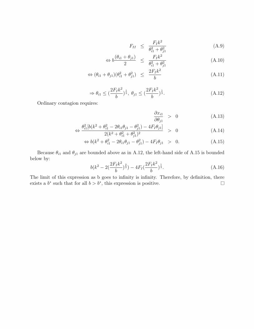
F

II

F

I

k

2

✓

2i1 + ✓

2j1

(A.9)

, b

(✓

i1 + ✓

j1)

2

F

I

k

2

✓

2i1 + ✓

2j1

(A.10)

, (✓

i1 + ✓

j1)(✓2i1 + ✓

2j1) 2F

I

k

2

b

(A.11)

) ✓

i1 (

2F

I

k

2

b

)

13, ✓

j1 (

2F

I

k

2

b

)

13. (A.12)

Ordinary contagion requires:

@x

i1

@✓

j1> 0 (A.13)

,✓

2i1[b(k

2+ ✓

2i1 � 2✓

i1✓j1 � ✓

2j1)� 4F

I

✓

j1]

2(k

2+ ✓

2i1 + ✓

2j1)

2> 0 (A.14)

, b(k

2+ ✓

2i1 � 2✓

i1✓j1 � ✓

2j1)� 4F

I

✓

j1 > 0. (A.15)

Because ✓

i1 and ✓

j1 are bounded above as in A.12, the left-hand side of A.15 is boundedbelow by:

b(k

2 � 2(

2F

I

k

2

b

)

23)� 4F

I

(

2F

I

k

2

b

)

13. (A.16)

The limit of this expression as b goes to infinity is infinity. Therefore, by definition, thereexists a b

⇤ such that for all b > b

⇤, this expression is positive.

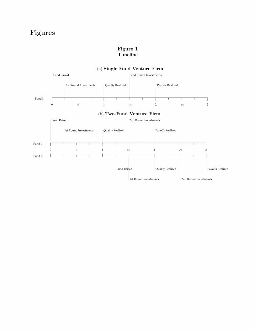
Figures

Figure 1Timeline

(a) Single-Fund Venture Firm

Fund II

Payoffs RealizedQuality Realized

2nd Round Investments1st Round Investments

Fund Raised

Fund I0 1 2 3

Fund Raised

1st Round Investments Quality Realized

2nd Round Investments

Payoffs Realized

½ 1½ 2½

(b) Two-Fund Venture Firm

Fund II

Payoffs RealizedQuality Realized

2nd Round Investments1st Round Investments

Fund Raised

Fund I0 1 2 3

Fund Raised

1st Round Investments Quality Realized

2nd Round Investments

Payoffs Realized

½ 1½ 2½

Figure 2The Technology Bubble and Venture Capital

This figure shows buy-and-hold returns on publicly traded internet stocks alongside quarterly flows to venturecapital funds. Internet stock returns are calculated as in Brunnermeier and Nagel (2004), using a value-weighted portfolio of stocks in the highest Nasdaq price/sales quintile, rebalanced monthly. Aggregatequarterly flows data are from Thomson. Flows in this case refers to commitments by limited partnersto newly raised venture funds. Only U.S. based funds structured as independent private partnerships areincluded. Both total flows as well as flows to internet-specific funds (as categorized by Thomson) are shown.Flows are converted to real 2000 dollars using the GDP deflator. The vertical line corresponds to the peakof all three series and is located at March 31, 2000.

02

46

8In

tern

et V

C F

low

s (B

illion

s)

010

2030

40Al

l VC

Flo

ws

(Billi

ons)

100%

200%

300%

400%

500%

Buy-

and-

Hol

d R

etur

n

1997 1998 1999 2000 2001 2002 2003

Internet Stocks All VC FundsInternet VC Funds

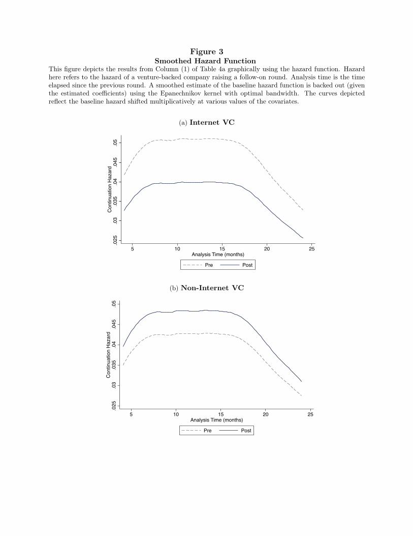
Figure 3Smoothed Hazard Function

This figure depicts the results from Column (1) of Table 4a graphically using the hazard function. Hazardhere refers to the hazard of a venture-backed company raising a follow-on round. Analysis time is the timeelapsed since the previous round. A smoothed estimate of the baseline hazard function is backed out (giventhe estimated coefficients) using the Epanechnikov kernel with optimal bandwidth. The curves depictedreflect the baseline hazard shifted multiplicatively at various values of the covariates.

(a) Internet VC.0

25.0

3.0

35.0

4.0

45.0

5C

ontin

uatio

n H

azar

d

5 10 15 20 25Analysis Time (months)

Pre Post

(b) Non-Internet VC

.025

.03

.035

.04

.045

.05

Con

tinua

tion

Haz

ard

5 10 15 20 25Analysis Time (months)

Pre Post

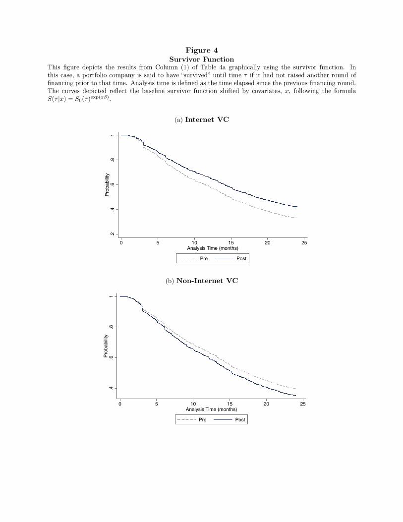
Figure 4Survivor Function

This figure depicts the results from Column (1) of Table 4a graphically using the survivor function. Inthis case, a portfolio company is said to have “survived” until time ⌧ if it had not raised another round offinancing prior to that time. Analysis time is defined as the time elapsed since the previous financing round.The curves depicted reflect the baseline survivor function shifted by covariates, x, following the formulaS(⌧ |x) = S

0

(⌧)

exp(x�)

.

(a) Internet VC.2

.4.6

.81

Prob

abilit

y

0 5 10 15 20 25Analysis Time (months)

Pre Post

(b) Non-Internet VC

.4.6

.81

Prob

abilit

y

0 5 10 15 20 25Analysis Time (months)

Pre Post

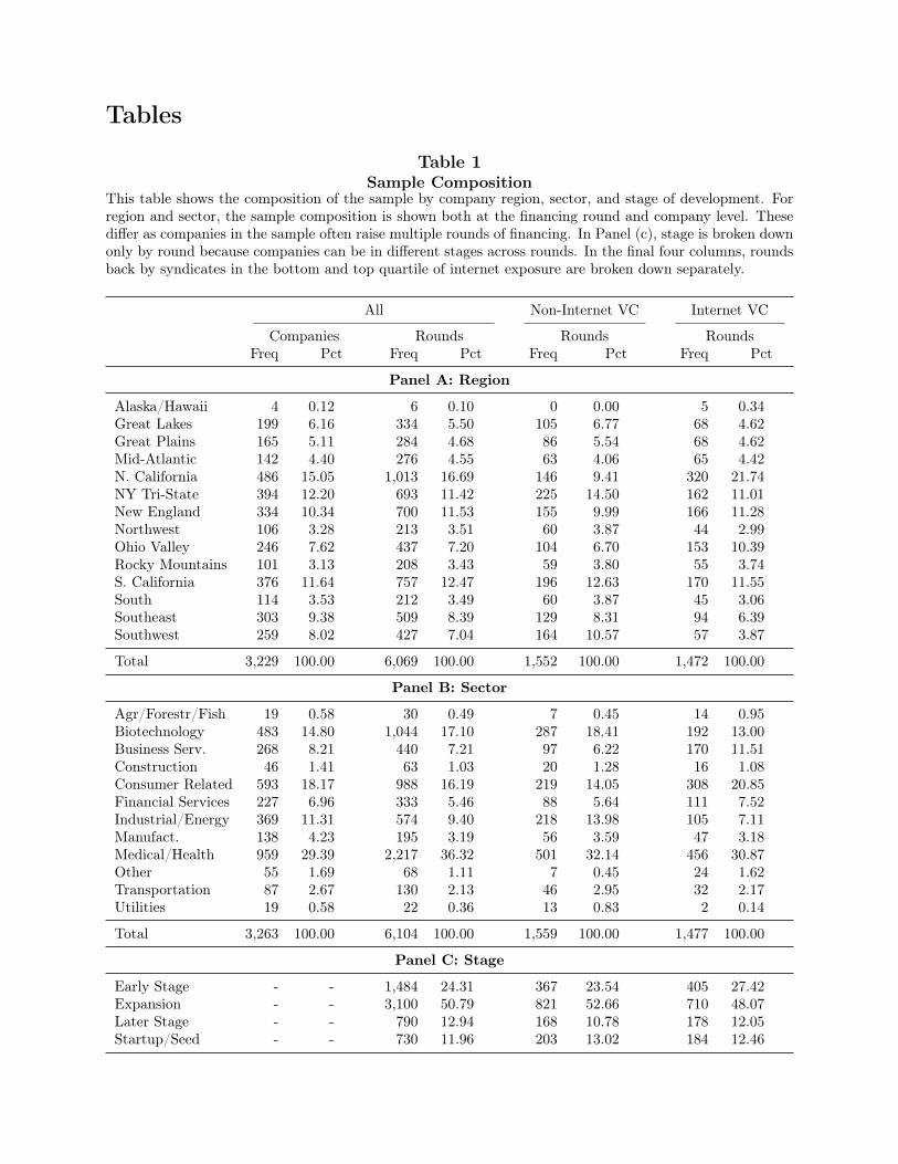
Tables

Table 1Sample Composition

This table shows the composition of the sample by company region, sector, and stage of development. Forregion and sector, the sample composition is shown both at the financing round and company level. Thesediffer as companies in the sample often raise multiple rounds of financing. In Panel (c), stage is broken downonly by round because companies can be in different stages across rounds. In the final four columns, roundsback by syndicates in the bottom and top quartile of internet exposure are broken down separately.

All Non-Internet VC Internet VC

Companies Rounds Rounds RoundsFreq Pct Freq Pct Freq Pct Freq Pct

Panel A: Region

Alaska/Hawaii 4 0.12 6 0.10 0 0.00 5 0.34

Great Lakes 199 6.16 334 5.50 105 6.77 68 4.62

Great Plains 165 5.11 284 4.68 86 5.54 68 4.62

Mid-Atlantic 142 4.40 276 4.55 63 4.06 65 4.42

N. California 486 15.05 1,013 16.69 146 9.41 320 21.74

NY Tri-State 394 12.20 693 11.42 225 14.50 162 11.01

New England 334 10.34 700 11.53 155 9.99 166 11.28

Northwest 106 3.28 213 3.51 60 3.87 44 2.99

Ohio Valley 246 7.62 437 7.20 104 6.70 153 10.39

Rocky Mountains 101 3.13 208 3.43 59 3.80 55 3.74

S. California 376 11.64 757 12.47 196 12.63 170 11.55

South 114 3.53 212 3.49 60 3.87 45 3.06

Southeast 303 9.38 509 8.39 129 8.31 94 6.39

Southwest 259 8.02 427 7.04 164 10.57 57 3.87

Total 3,229 100.00 6,069 100.00 1,552 100.00 1,472 100.00

Panel B: Sector

Agr/Forestr/Fish 19 0.58 30 0.49 7 0.45 14 0.95

Biotechnology 483 14.80 1,044 17.10 287 18.41 192 13.00

Business Serv. 268 8.21 440 7.21 97 6.22 170 11.51

Construction 46 1.41 63 1.03 20 1.28 16 1.08

Consumer Related 593 18.17 988 16.19 219 14.05 308 20.85

Financial Services 227 6.96 333 5.46 88 5.64 111 7.52

Industrial/Energy 369 11.31 574 9.40 218 13.98 105 7.11

Manufact. 138 4.23 195 3.19 56 3.59 47 3.18

Medical/Health 959 29.39 2,217 36.32 501 32.14 456 30.87

Other 55 1.69 68 1.11 7 0.45 24 1.62

Transportation 87 2.67 130 2.13 46 2.95 32 2.17

Utilities 19 0.58 22 0.36 13 0.83 2 0.14

Total 3,263 100.00 6,104 100.00 1,559 100.00 1,477 100.00

Panel C: Stage

Early Stage - - 1,484 24.31 367 23.54 405 27.42

Expansion - - 3,100 50.79 821 52.66 710 48.07

Later Stage - - 790 12.94 168 10.78 178 12.05

Startup/Seed - - 730 11.96 203 13.02 184 12.46

Total - - 6,104 100.00 1,559 100.00 1,477 100.00

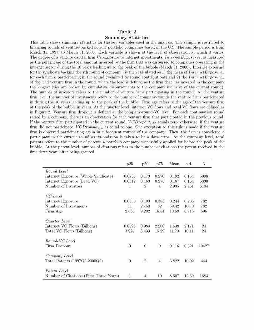
Table 2Summary Statistics

This table shows summary statistics for the key variables used in the analysis. The sample is restricted tofinancing rounds of venture-backed non-IT portfolio companies based in the U.S. The sample period is fromMarch 31, 1997, to March 31, 2003. Each variable is shown at the level of observation at which it varies.The degree of a venture capital firm k’s exposure to internet investments, InternetExposure

k

, is measuredas the percentage of the total amount invested by the firm that was disbursed to companies operating in theinternet sector during the 10 years leading up to the peak of the bubble (March 31, 2000). Internet exposurefor the syndicate backing the jth round of company i is then calculated as 1) the mean of InternetExposure

k

for each firm k participating in the round (weighted by round contributions) and 2) the InternetExposure

k

of the lead venture firm in the round, where the lead is defined as the firm that has invested in the companythe longest (ties are broken by cumulative disbursements to the company inclusive of the current round).The number of investors refers to the number of venture firms participating in the round. At the venturefirm level, the number of investments refers to the number of company-rounds the venture firms participatedin during the 10 years leading up to the peak of the bubble. Firm age refers to the age of the venture firmat the peak of the bubble in years. At the quarter level, internet VC flows and total VC flows are defined asin Figure 2. Venture firm dropout is defined at the company-round-VC level. For each continuation roundraised by a company, there is an observation for each venture firm that participated in the previous round.If the venture firm participated in the current round, V CDropout

ijkt

equals zero; otherwise, if the venturefirm did not participate, V CDropout

ijkt

is equal to one. One exception to this rule is made if the venturefirm is observed participating again in subsequent rounds of the company. Then, the firm is considered aparticipant in the current round as its omission is taken to be a data error. At the company level, totalpatents refers to the number of patents a portfolio company successfully applied for before the peak of thebubble. At the patent level, number of citations refers to the number of citations the patent received in thefirst three years after being granted.

p25 p50 p75 Mean s.d. N

Round Level

Internet Exposure (Whole Syndicate) 0.0735 0.173 0.270 0.192 0.154 5908Internet Exposure (Lead VC) 0.0512 0.163 0.275 0.187 0.164 5330Number of Investors 1 2 4 2.935 2.461 6104

VC Level

Internet Exposure 0.0330 0.193 0.383 0.244 0.235 782Number of Investments 11 25.50 62 59.42 100.0 782Firm Age 2.836 9.292 16.54 10.59 8.915 596

Quarter Level

Internet VC Flows (Billions) 0.0596 0.980 2.206 1.638 2.171 24Total VC Flows (Billions) 3.924 8.433 15.29 11.73 10.11 24

Round-VC Level

Firm Dropout 0 0 0 0.116 0.321 10427

Company Level

Total Patents (1997Q2-2000Q2) 0 2 4 3.822 10.92 444

Patent Level

Number of Citations (First Three Years) 1 4 10 8.607 12.69 1683

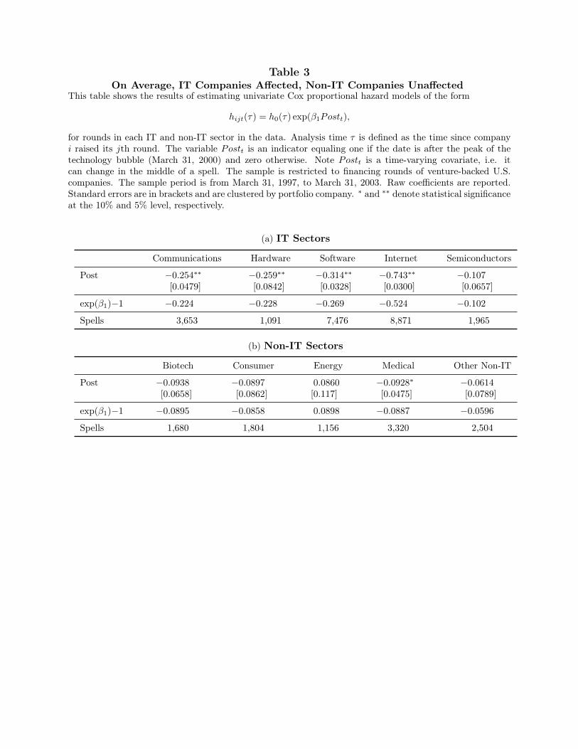
Table 3On Average, IT Companies Affected, Non-IT Companies Unaffected

This table shows the results of estimating univariate Cox proportional hazard models of the form

h

ijt

(⌧) = h

0

(⌧) exp(�

1

Post

t

),

for rounds in each IT and non-IT sector in the data. Analysis time ⌧ is defined as the time since companyi raised its jth round. The variable Post

t

is an indicator equaling one if the date is after the peak of thetechnology bubble (March 31, 2000) and zero otherwise. Note Post

t

is a time-varying covariate, i.e. itcan change in the middle of a spell. The sample is restricted to financing rounds of venture-backed U.S.companies. The sample period is from March 31, 1997, to March 31, 2003. Raw coefficients are reported.Standard errors are in brackets and are clustered by portfolio company. ⇤ and ⇤⇤ denote statistical significanceat the 10% and 5% level, respectively.

(a) IT Sectors

Communications Hardware Software Internet Semiconductors

Post �0.254

⇤⇤ �0.259

⇤⇤ �0.314

⇤⇤ �0.743

⇤⇤ �0.107

[0.0479] [0.0842] [0.0328] [0.0300] [0.0657]

exp(�1

)�1 �0.224 �0.228 �0.269 �0.524 �0.102

Spells 3,653 1,091 7,476 8,871 1,965

(b) Non-IT Sectors

Biotech Consumer Energy Medical Other Non-IT

Post �0.0938 �0.0897 0.0860 �0.0928

⇤ �0.0614

[0.0658] [0.0862] [0.117] [0.0475] [0.0789]

exp(�1

)�1 �0.0895 �0.0858 0.0898 �0.0887 �0.0596

Spells 1,680 1,804 1,156 3,320 2,504

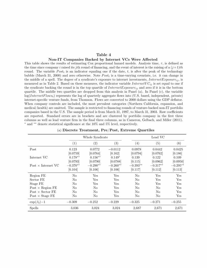
Table 4Non-IT Companies Backed by Internet VCs Were Affected

This table shows the results of estimating Cox proportional hazard models. Analysis time, ⌧ , is defined asthe time since company i raised its jth round of financing, and the event of interest is the raising of a (j+1)th

round. The variable Post

t

is an indicator equaling one if the date, t, is after the peak of the technologybubble (March 31, 2000) and zero otherwise. Note Post

t

is a time-varying covariate, i.e. it can change inthe middle of a spell. The degree of a syndicate’s exposure to internet investments, InternetExposure

ij

, ismeasured as in Table 2. Based on these measures, the indicator variable InternetV C

ij

is set equal to one ifthe syndicate backing the round is in the top quartile of InternetExposure

ij

and zero if it is in the bottomquartile. The middle two quartiles are dropped from this analysis in Panel (a). In Panel (c), the variablelog(InternetF lows

t

) represents the log of quarterly aggregate flows into (U.S. based, independent, private)internet-specific venture funds, from Thomson. Flows are converted to 2000 dollars using the GDP deflator.When company controls are included, the most prevalent categories (Northern California, expansion, andmedical/health) are omitted. The sample is restricted to financing rounds of venture-backed non-IT portfoliocompanies based in the U.S. The sample period is from March 31, 1997, to March 31, 2003. Raw coefficientsare reported. Standard errors are in brackets and are clustered by portfolio company in the first threecolumns as well as lead venture firm in the final three columns, as in Cameron, Gelbach, and Miller (2011).⇤ and ⇤⇤ denote statistical significance at the 10% and 5% level, respectively.

(a) Discrete Treatment, Pre/Post, Extreme Quartiles

Whole Syndicate Lead VC

(1) (2) (3) (4) (5) (6)

Post 0.123 0.0772 �0.0112 0.0978 0.0442 0.0425

[0.0759] [0.0764] [0.162] [0.0794] [0.0762] [0.186]

Internet VC 0.178

⇤⇤0.156

⇤⇤0.149

⇤0.139 0.122 0.109

[0.0793] [0.0790] [0.0788] [0.115] [0.0962] [0.0950]

Post ⇥ Internet VC �0.370

⇤⇤ �0.290

⇤⇤ �0.260

⇤⇤ �0.393

⇤⇤ �0.317

⇤⇤ �0.295

⇤⇤

[0.104] [0.106] [0.106] [0.117] [0.112] [0.113]

Region FE No Yes Yes No Yes YesSector FE No Yes Yes No Yes YesStage FE No Yes Yes No Yes YesPost ⇥ Region FE No No Yes No No YesPost ⇥ Sector FE No No Yes No No YesPost ⇥ Stage FE No No Yes No No Yes

exp(�3

)�1 �0.309 �0.252 �0.229 �0.325 �0.271 �0.255

Spells 3,036 3,024 3,024 2,687 2,671 2,671

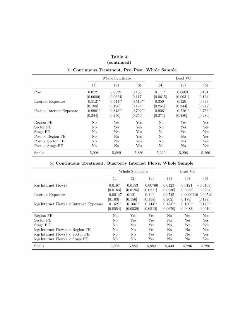
Table 4(continued)

(b) Continuous Treatment, Pre/Post, Whole Sample

Whole Syndicate Lead VC

(1) (2) (3) (4) (5) (6)

Post 0.0721 0.0579 0.105 0.111

⇤0.0803 0.191

[0.0600] [0.0624] [0.117] [0.0615] [0.0631] [0.134]

Internet Exposure 0.512

⇤⇤0.541

⇤⇤0.519

⇤⇤0.359 0.329 0.343

[0.188] [0.196] [0.194] [0.254] [0.244] [0.242]

Post ⇥ Internet Exposure �0.996

⇤⇤ �0.848

⇤⇤ �0.792

⇤⇤ �0.906

⇤⇤ �0.726

⇤⇤ �0.753

⇤⇤

[0.244] [0.256] [0.256] [0.271] [0.280] [0.280]

Region FE No Yes Yes No Yes YesSector FE No Yes Yes No Yes YesStage FE No Yes Yes No Yes YesPost ⇥ Region FE No No Yes No No YesPost ⇥ Sector FE No No Yes No No YesPost ⇥ Stage FE No No Yes No No Yes

Spells 5,908 5,889 5,889 5,330 5,296 5,296

(c) Continuous Treatment, Quarterly Internet Flows, Whole Sample

Whole Syndicate Lead VC

(1) (2) (3) (4) (5) (6)

log(Internet Flows) 0.0167 0.0153 0.00760 0.0123 0.0124 �0.0103

[0.0183] [0.0195] [0.0271] [0.0230] [0.0238] [0.0267]

Internet Exposure 0.00147 0.121 0.111 �0.0745 �0.0000116 0.00549

[0.163] [0.156] [0.155] [0.202] [0.179] [0.178]

log(Internet Flows) ⇥ Internet Exposure 0.162

⇤⇤0.166

⇤⇤0.144

⇤⇤0.183

⇤⇤0.180

⇤⇤0.175

⇤⇤

[0.0554] [0.0539] [0.0512] [0.0679] [0.0683] [0.0619]

Region FE No Yes Yes No Yes YesSector FE No Yes Yes No Yes YesStage FE No Yes Yes No Yes Yeslog(Internet Flows) ⇥ Region FE No No Yes No No Yeslog(Internet Flows) ⇥ Sector FE No No Yes No No Yeslog(Internet Flows) ⇥ Stage FE No No Yes No No Yes

Spells 5,908 5,889 5,889 5,330 5,296 5,296

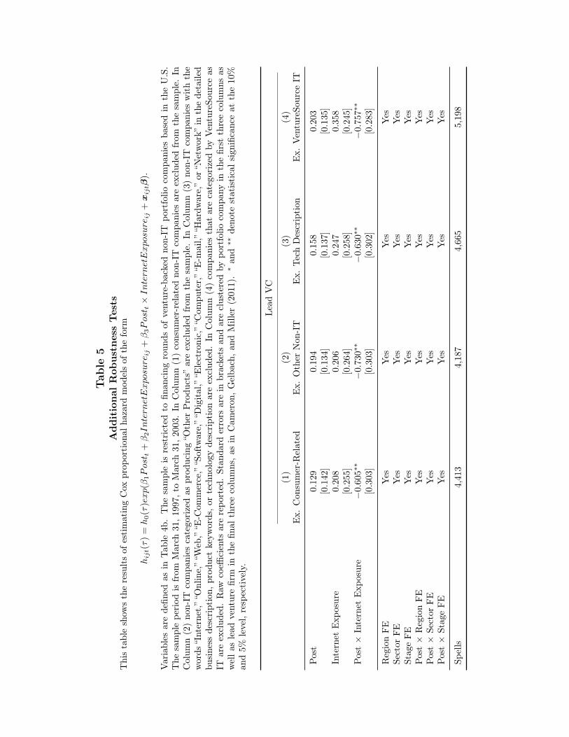
Tab

le5

Add

itio

nalR

obus

tnes

sTes

tsT

his

tabl

esh

ows

the

resu

lts

ofes

tim

atin

gC

oxpr

opor

tion

alha

zard

mod

els

ofth

efo

rm

h

ijt

(⌧)=

h

0

(⌧)exp(�

1

Post

t

+�

2

InternetExposure

ij

+�

3

Post

t

⇥InternetExposure

ij

+x

ijt

�).

Var

iabl

esar

ede

fined

asin

Tabl

e4b

.T

hesa

mpl

eis

rest

rict

edto

finan

cing

roun

dsof

vent

ure-

back

edno

n-IT

port

folio

com

pani

esba

sed

inth

eU

.S.

The

sam

ple

peri

odis

from

Mar

ch31

,199

7,to

Mar

ch31

,200

3.In

Col

umn

(1)

cons

umer

-rel

ated

non-

ITco

mpa

nies

are

excl

uded

from

the

sam

ple.

InC

olum

n(2

)no

n-IT

com

pani

esca

tego

rize

das

prod

ucin

g“O

ther

Pro

duct

s”ar

eex

clud

edfr

omth

esa

mpl

e.In

Col

umn

(3)

non-

ITco

mpa

nies

wit

hth

ew

ords

“Int

erne

t,”

“Onl

ine,

”“W

eb,”

“E-C

omm

erce

,”“S

oftw

are,

”“D

igit

al,”

“Ele

ctro

nic,

”“C

ompu

ter,

”“E

-mai

l,”“H

ardw

are,

”or

“Net

wor

k”in

the

deta

iled

busi

ness

desc

ript

ion,

prod

uct

keyw

ords

,or

tech

nolo

gyde

scri

ptio

nar

eex

clud

ed.

InC

olum

n(4

)co

mpa

nies

that

are

cate

gori

zed

byV

entu

reSo

urce

asIT

are

excl

uded

.R

awco

effici

ents

are

repo

rted

.St

anda

rder

rors

are

inbr

acke

tsan

dar

ecl

uste

red

bypo

rtfo

lioco

mpa

nyin

the

first

thre

eco

lum

nsas

wel

las

lead

vent

ure

firm

inth

efin

alth

ree

colu

mns

,as

inC

amer

on,G

elba

ch,a

ndM

iller

(201

1).

⇤an

d⇤⇤

deno

test

atis

tica

lsig

nific

ance

atth

e10

%an

d5%

leve

l,re

spec

tive

ly.

Lead

VC

(1)

(2)

(3)

(4)

Ex.

Con

sum

er-R

elat

edE

x.O

ther

Non

-IT

Ex.

Tech

Des

crip

tion

Ex.

Ven

ture

Sour

ceIT

Post

0.129

0.194

0.158

0.203

[0.142]

[0.134]

[0.137]

[0.135]

Inte

rnet

Exp

osur

e0.208

0.206

0.247

0.358

[0.255]

[0.264]

[0.258]

[0.245]

Post

⇥In

tern

etE

xpos

ure

�0.605

⇤⇤�0.730

⇤⇤�0.630

⇤⇤�0.757

⇤⇤

[0.303]

[0.303]

[0.302]

[0.283]

Reg

ion

FEY

esYes

Yes

Yes

Sect

orFE

Yes

Yes

Yes

Yes

Stag

eFE

Yes

Yes

Yes

Yes

Post

⇥R

egio

nFE

Yes

Yes

Yes

Yes

Post

⇥Se

ctor

FEY

esY

esY

esY

esPo

st⇥

Stag

eFE

Yes

Yes

Yes

Yes

Spel

ls4,

413

4,18

74,

665

5,19

8

Table 6Continuation Hazard Did Not Increase as Bubble Inflated, Decreased as Deflated

This table shows the results of estimating Cox proportional hazard models of the form

h

ijt

(⌧) = h

0

(⌧)exp(�

1

log(InternetF lows

t

) + �

2

InternetExposure

ij

+

�

3

log(InternetF lows

t

)⇥ InternetExposure

ij

+

�

4

log(InternetF lows

t

)⇥ InternetExposure

ij

⇥ Post

t

+ x

ijt

�).

Analysis time, ⌧ , is defined as the time since company i raised its jth round. The variablelog(InternetF lows

t

) represents the log of quarterly aggregate flows into (U.S. based, independent, pri-vate) internet-specific venture funds, from Thomson. All other variables are defined as in Table 4. Whencompany controls are included, the most prevalent categories (Northern California, expansion, and medi-cal/health) are omitted. The sample is restricted to financing rounds of venture-backed non-IT portfoliocompanies based in the U.S. The sample period is from March 31, 1997, to March 31, 2003. Raw coefficientsare reported. Standard errors are in brackets and are clustered by portfolio company and quarter in the firstthree columns as well as lead venture firm in the final three columns, as in Cameron, Gelbach, and Miller(2011). ⇤ and ⇤⇤ denote statistical significance at the 10% and 5% level, respectively.

Whole Syndicate Lead VC

(1) (2) (3) (4) (5) (6)

log(Internet Flows) 0.0199 0.0186 0.00894 0.0156 0.0158 �0.00925

[0.0173] [0.0185] [0.0269] [0.0225] [0.0232] [0.0269]

Internet Exposure 0.0266 0.148 0.137 �0.0500 0.0253 0.0317

[0.170] [0.165] [0.163] [0.204] [0.184] [0.184]

log(Internet Flows) ⇥ Internet Exposure �0.0555 �0.0581 �0.0793 �0.0693 �0.0792 �0.0880

[0.0930] [0.0896] [0.0856] [0.105] [0.105] [0.100]

log(Internet Flows) ⇥ Internet Exposure ⇥Post

0.287

⇤⇤0.299

⇤⇤0.297

⇤⇤0.340

⇤⇤0.352

⇤⇤0.354

⇤⇤

[0.106] [0.101] [0.0984] [0.109] [0.104] [0.102]

Region FE No Yes Yes No Yes YesSector FE No Yes Yes No Yes YesStage FE No Yes Yes No Yes Yeslog(Internet Flows) ⇥ Region FE No No Yes No No Yeslog(Internet Flows) ⇥ Sector FE No No Yes No No Yeslog(Internet Flows) ⇥ Stage FE No No Yes No No Yes

Spells 5,908 5,889 5,889 5,330 5,296 5,296

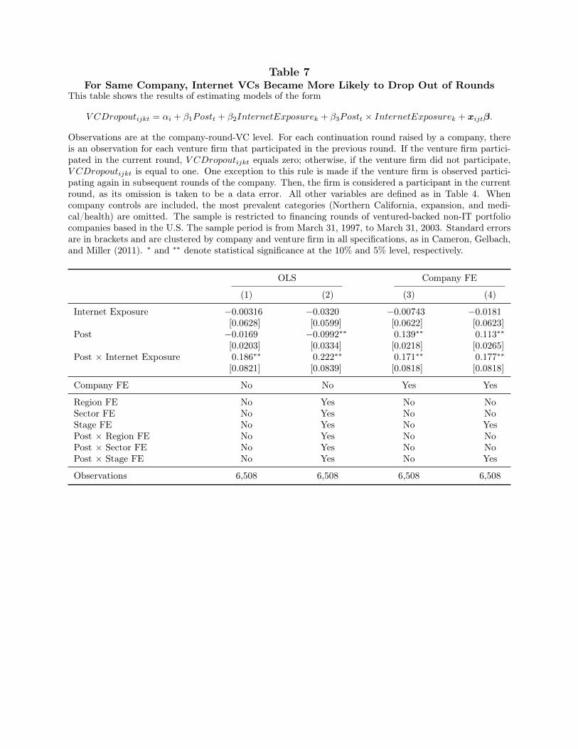
Table 7For Same Company, Internet VCs Became More Likely to Drop Out of Rounds

This table shows the results of estimating models of the form

V CDropout

ijkt

= ↵

i

+ �

1

Post

t

+ �

2

InternetExposure

k

+ �

3

Post

t

⇥ InternetExposure

k

+ x

ijt

�.

Observations are at the company-round-VC level. For each continuation round raised by a company, thereis an observation for each venture firm that participated in the previous round. If the venture firm partici-pated in the current round, V CDropout

ijkt

equals zero; otherwise, if the venture firm did not participate,V CDropout

ijkt

is equal to one. One exception to this rule is made if the venture firm is observed partici-pating again in subsequent rounds of the company. Then, the firm is considered a participant in the currentround, as its omission is taken to be a data error. All other variables are defined as in Table 4. Whencompany controls are included, the most prevalent categories (Northern California, expansion, and medi-cal/health) are omitted. The sample is restricted to financing rounds of ventured-backed non-IT portfoliocompanies based in the U.S. The sample period is from March 31, 1997, to March 31, 2003. Standard errorsare in brackets and are clustered by company and venture firm in all specifications, as in Cameron, Gelbach,and Miller (2011). ⇤ and ⇤⇤ denote statistical significance at the 10% and 5% level, respectively.

OLS Company FE

(1) (2) (3) (4)

Internet Exposure �0.00316 �0.0320 �0.00743 �0.0181

[0.0628] [0.0599] [0.0622] [0.0623]

Post �0.0169 �0.0992

⇤⇤0.139

⇤⇤0.113

⇤⇤

[0.0203] [0.0334] [0.0218] [0.0265]

Post ⇥ Internet Exposure 0.186

⇤⇤0.222

⇤⇤0.171

⇤⇤0.177

⇤⇤

[0.0821] [0.0839] [0.0818] [0.0818]

Company FE No No Yes Yes

Region FE No Yes No NoSector FE No Yes No NoStage FE No Yes No YesPost ⇥ Region FE No Yes No NoPost ⇥ Sector FE No Yes No NoPost ⇥ Stage FE No Yes No Yes

Observations 6,508 6,508 6,508 6,508

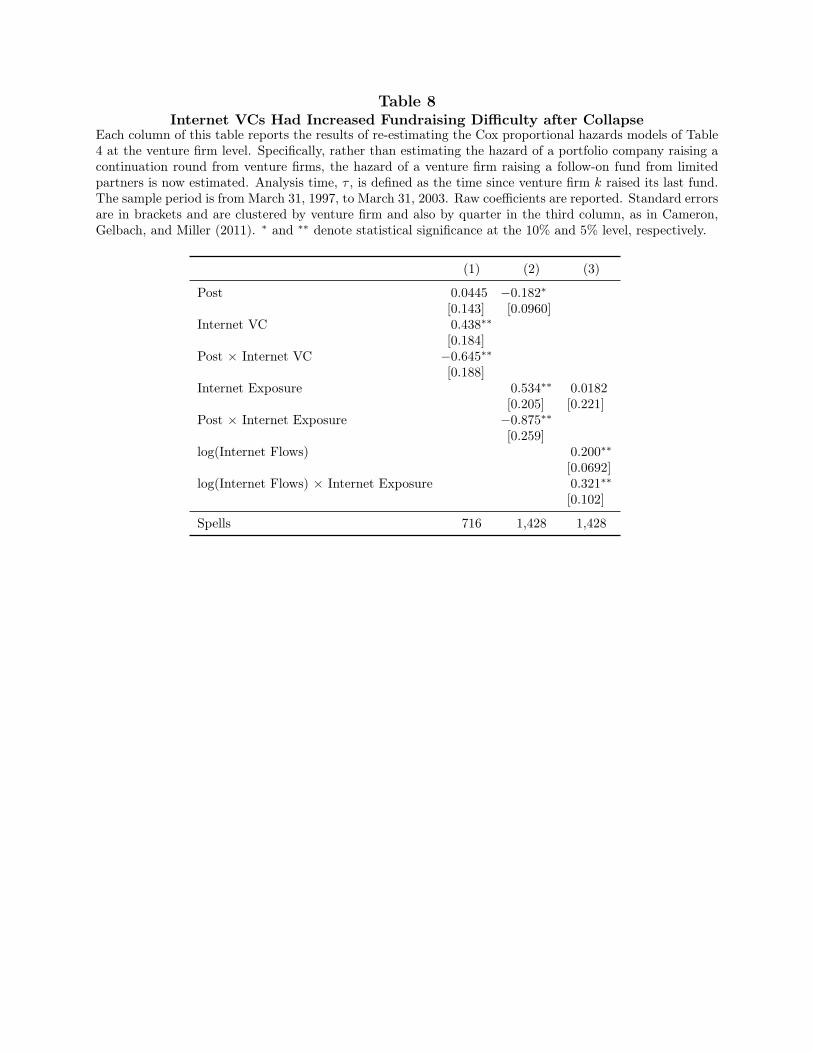
Table 8Internet VCs Had Increased Fundraising Difficulty after Collapse

Each column of this table reports the results of re-estimating the Cox proportional hazards models of Table4 at the venture firm level. Specifically, rather than estimating the hazard of a portfolio company raising acontinuation round from venture firms, the hazard of a venture firm raising a follow-on fund from limitedpartners is now estimated. Analysis time, ⌧ , is defined as the time since venture firm k raised its last fund.The sample period is from March 31, 1997, to March 31, 2003. Raw coefficients are reported. Standard errorsare in brackets and are clustered by venture firm and also by quarter in the third column, as in Cameron,Gelbach, and Miller (2011). ⇤ and ⇤⇤ denote statistical significance at the 10% and 5% level, respectively.

(1) (2) (3)

Post 0.0445 �0.182

⇤

[0.143] [0.0960]

Internet VC 0.438

⇤⇤

[0.184]

Post ⇥ Internet VC �0.645

⇤⇤

[0.188]

Internet Exposure 0.534

⇤⇤0.0182

[0.205] [0.221]

Post ⇥ Internet Exposure �0.875

⇤⇤

[0.259]

log(Internet Flows) 0.200

⇤⇤

[0.0692]

log(Internet Flows) ⇥ Internet Exposure 0.321

⇤⇤

[0.102]

Spells 716 1,428 1,428

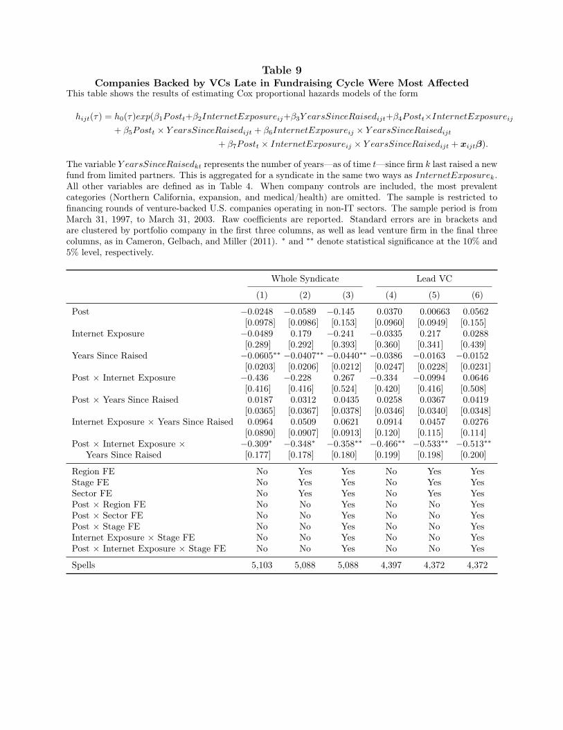
Table 9Companies Backed by VCs Late in Fundraising Cycle Were Most Affected

This table shows the results of estimating Cox proportional hazards models of the form

h

ijt

(⌧) = h

0

(⌧)exp(�

1

Post

t

+�

2

InternetExposure

ij

+�

3

Y earsSinceRaised

ijt

+�

4

Post

t

⇥InternetExposure

ij

+ �

5

Post

t

⇥ Y earsSinceRaised

ijt

+ �

6

InternetExposure

ij

⇥ Y earsSinceRaised

ijt

+ �

7

Post

t

⇥ InternetExposure

ij

⇥ Y earsSinceRaised

ijt

+ x

ijt

�).

The variable Y earsSinceRaised

kt

represents the number of years—as of time t—since firm k last raised a newfund from limited partners. This is aggregated for a syndicate in the same two ways as InternetExposure

k

.All other variables are defined as in Table 4. When company controls are included, the most prevalentcategories (Northern California, expansion, and medical/health) are omitted. The sample is restricted tofinancing rounds of venture-backed U.S. companies operating in non-IT sectors. The sample period is fromMarch 31, 1997, to March 31, 2003. Raw coefficients are reported. Standard errors are in brackets andare clustered by portfolio company in the first three columns, as well as lead venture firm in the final threecolumns, as in Cameron, Gelbach, and Miller (2011). ⇤ and ⇤⇤ denote statistical significance at the 10% and5% level, respectively.

Whole Syndicate Lead VC

(1) (2) (3) (4) (5) (6)

Post �0.0248 �0.0589 �0.145 0.0370 0.00663 0.0562

[0.0978] [0.0986] [0.153] [0.0960] [0.0949] [0.155]

Internet Exposure �0.0489 0.179 �0.241 �0.0335 0.217 0.0288

[0.289] [0.292] [0.393] [0.360] [0.341] [0.439]

Years Since Raised �0.0605

⇤⇤ �0.0407

⇤⇤ �0.0440

⇤⇤ �0.0386 �0.0163 �0.0152

[0.0203] [0.0206] [0.0212] [0.0247] [0.0228] [0.0231]

Post ⇥ Internet Exposure �0.436 �0.228 0.267 �0.334 �0.0994 0.0646

[0.416] [0.416] [0.524] [0.420] [0.416] [0.508]

Post ⇥ Years Since Raised 0.0187 0.0312 0.0435 0.0258 0.0367 0.0419

[0.0365] [0.0367] [0.0378] [0.0346] [0.0340] [0.0348]

Internet Exposure ⇥ Years Since Raised 0.0964 0.0509 0.0621 0.0914 0.0457 0.0276

[0.0890] [0.0907] [0.0913] [0.120] [0.115] [0.114]

Post ⇥ Internet Exposure ⇥Years Since Raised

�0.309

⇤ �0.348

⇤ �0.358

⇤⇤ �0.466

⇤⇤ �0.533

⇤⇤ �0.513

⇤⇤

[0.177] [0.178] [0.180] [0.199] [0.198] [0.200]

Region FE No Yes Yes No Yes YesStage FE No Yes Yes No Yes YesSector FE No Yes Yes No Yes YesPost ⇥ Region FE No No Yes No No YesPost ⇥ Sector FE No No Yes No No YesPost ⇥ Stage FE No No Yes No No YesInternet Exposure ⇥ Stage FE No No Yes No No YesPost ⇥ Internet Exposure ⇥ Stage FE No No Yes No No Yes

Spells 5,103 5,088 5,088 4,397 4,372 4,372

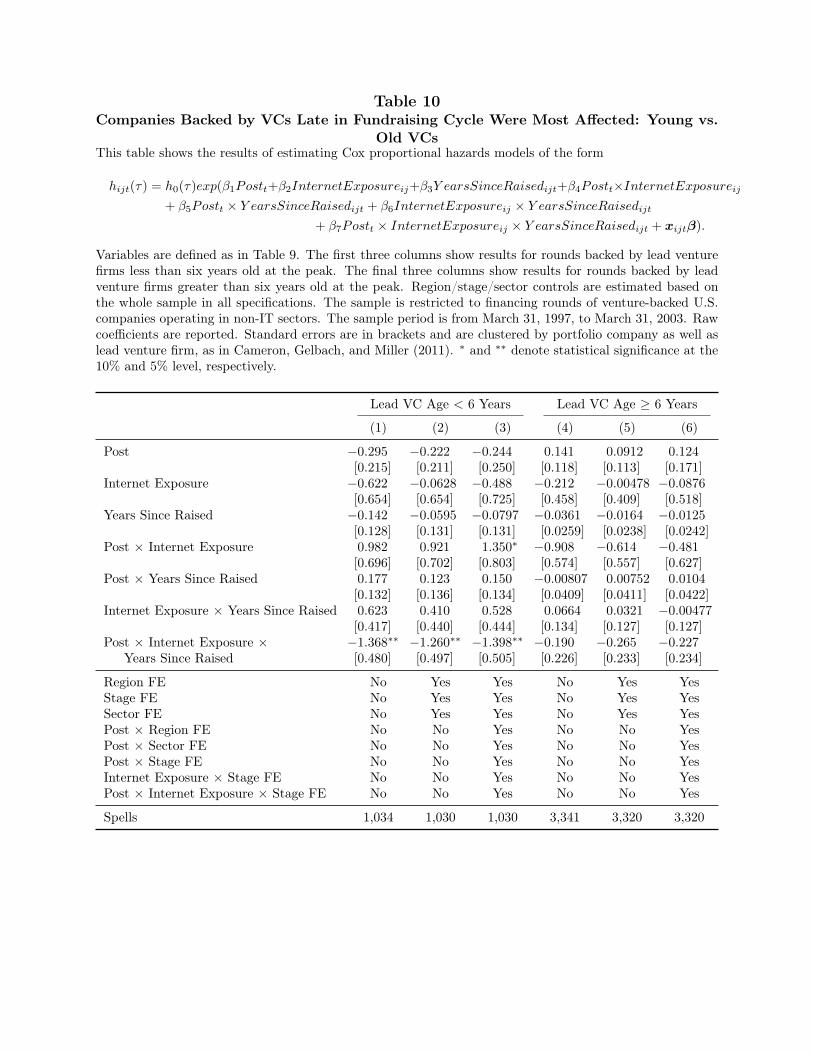
Table 10Companies Backed by VCs Late in Fundraising Cycle Were Most Affected: Young vs.

Old VCsThis table shows the results of estimating Cox proportional hazards models of the form

h

ijt

(⌧) = h

0

(⌧)exp(�

1

Post

t

+�

2

InternetExposure

ij

+�

3

Y earsSinceRaised

ijt

+�

4

Post

t

⇥InternetExposure

ij

+ �

5

Post

t

⇥ Y earsSinceRaised

ijt

+ �

6

InternetExposure

ij

⇥ Y earsSinceRaised

ijt

+ �

7

Post

t

⇥ InternetExposure

ij

⇥ Y earsSinceRaised

ijt

+ x

ijt

�).

Variables are defined as in Table 9. The first three columns show results for rounds backed by lead venturefirms less than six years old at the peak. The final three columns show results for rounds backed by leadventure firms greater than six years old at the peak. Region/stage/sector controls are estimated based onthe whole sample in all specifications. The sample is restricted to financing rounds of venture-backed U.S.companies operating in non-IT sectors. The sample period is from March 31, 1997, to March 31, 2003. Rawcoefficients are reported. Standard errors are in brackets and are clustered by portfolio company as well aslead venture firm, as in Cameron, Gelbach, and Miller (2011). ⇤ and ⇤⇤ denote statistical significance at the10% and 5% level, respectively.

Lead VC Age < 6 Years Lead VC Age � 6 Years

(1) (2) (3) (4) (5) (6)

Post �0.295 �0.222 �0.244 0.141 0.0912 0.124

[0.215] [0.211] [0.250] [0.118] [0.113] [0.171]

Internet Exposure �0.622 �0.0628 �0.488 �0.212 �0.00478 �0.0876

[0.654] [0.654] [0.725] [0.458] [0.409] [0.518]

Years Since Raised �0.142 �0.0595 �0.0797 �0.0361 �0.0164 �0.0125

[0.128] [0.131] [0.131] [0.0259] [0.0238] [0.0242]

Post ⇥ Internet Exposure 0.982 0.921 1.350

⇤ �0.908 �0.614 �0.481

[0.696] [0.702] [0.803] [0.574] [0.557] [0.627]

Post ⇥ Years Since Raised 0.177 0.123 0.150 �0.00807 0.00752 0.0104

[0.132] [0.136] [0.134] [0.0409] [0.0411] [0.0422]

Internet Exposure ⇥ Years Since Raised 0.623 0.410 0.528 0.0664 0.0321 �0.00477

[0.417] [0.440] [0.444] [0.134] [0.127] [0.127]

Post ⇥ Internet Exposure ⇥Years Since Raised

�1.368

⇤⇤ �1.260

⇤⇤ �1.398

⇤⇤ �0.190 �0.265 �0.227

[0.480] [0.497] [0.505] [0.226] [0.233] [0.234]

Region FE No Yes Yes No Yes YesStage FE No Yes Yes No Yes YesSector FE No Yes Yes No Yes YesPost ⇥ Region FE No No Yes No No YesPost ⇥ Sector FE No No Yes No No YesPost ⇥ Stage FE No No Yes No No YesInternet Exposure ⇥ Stage FE No No Yes No No YesPost ⇥ Internet Exposure ⇥ Stage FE No No Yes No No Yes

Spells 1,034 1,030 1,030 3,341 3,320 3,320

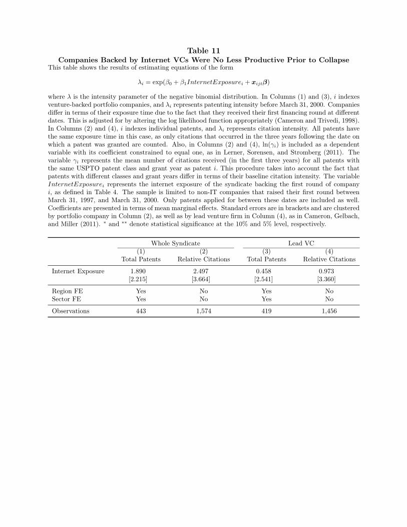
Table 11Companies Backed by Internet VCs Were No Less Productive Prior to Collapse

This table shows the results of estimating equations of the form

�

i

= exp(�

0

+ �

1

InternetExposure

i

+ x

ijt

�)

where � is the intensity parameter of the negative binomial distribution. In Columns (1) and (3), i indexesventure-backed portfolio companies, and �

i

represents patenting intensity before March 31, 2000. Companiesdiffer in terms of their exposure time due to the fact that they received their first financing round at differentdates. This is adjusted for by altering the log likelihood function appropriately (Cameron and Trivedi, 1998).In Columns (2) and (4), i indexes individual patents, and �

i

represents citation intensity. All patents havethe same exposure time in this case, as only citations that occurred in the three years following the date onwhich a patent was granted are counted. Also, in Columns (2) and (4), ln(�

i

) is included as a dependentvariable with its coefficient constrained to equal one, as in Lerner, Sorensen, and Stromberg (2011). Thevariable �

i

represents the mean number of citations received (in the first three years) for all patents withthe same USPTO patent class and grant year as patent i. This procedure takes into account the fact thatpatents with different classes and grant years differ in terms of their baseline citation intensity. The variableInternetExposure

i

represents the internet exposure of the syndicate backing the first round of companyi, as defined in Table 4. The sample is limited to non-IT companies that raised their first round betweenMarch 31, 1997, and March 31, 2000. Only patents applied for between these dates are included as well.Coefficients are presented in terms of mean marginal effects. Standard errors are in brackets and are clusteredby portfolio company in Column (2), as well as by lead venture firm in Column (4), as in Cameron, Gelbach,and Miller (2011). ⇤ and ⇤⇤ denote statistical significance at the 10% and 5% level, respectively.

Whole Syndicate Lead VC(1) (2) (3) (4)

Total Patents Relative Citations Total Patents Relative Citations

Internet Exposure 1.890 2.497 0.458 0.973

[2.215] [3.664] [2.541] [3.360]

Region FE Yes No Yes NoSector FE Yes No Yes No

Observations 443 1,574 419 1,456