Effects of Monetary Policy Shocks on Inequality in Japan Masayuki Inui† masayuki.inui@boj.or.jp Nao Sudo‡ nao.sudou@boj.or.jp Tomoaki Yamada§ tyamada@meiji.ac.jp

No.17-E-3 May 2017

Bank of Japan 2-1-1 Nihonbashi-Hongokucho, Chuo-ku, Tokyo 103-0021, Japan

† Monetary Affairs Department, Bank of Japan ‡ Monetary Affairs Department, Bank of Japan § School of Commerce, Meiji University

Papers in the Bank of Japan Working Paper Series are circulated in order to stimulate discussion and comments. Views expressed are those of authors and do not necessarily reflect those of the Bank. If you have any comment or question on the working paper series, please contact each author. When making a copy or reproduction of the content for commercial purposes, please contact the Public Relations Department (post.prd8@boj.or.jp) at the Bank in advance to request permission. When making a copy or reproduction, the source, Bank of Japan Working Paper Series, should explicitly be credited.

Bank of Japan Working Paper Series

1

Effects of Monetary Policy Shocks on Inequality in Japan

Masayuki Inui,† Nao Sudo,‡ and Tomoaki Yamada§

May 2017

Abstract

Impacts of monetary easing on inequality have recently attracted increasing attention. In this paper, we use the micro-level data of Japanese households to study the distributional effects of monetary policy. We construct quarterly series of income and consumption inequality measures from 1981 to 2008, and estimate their response to a monetary policy shock. We do find that monetary policy shocks do not have statistically significant impacts on inequalities across Japanese households in a stable manner. We find evidence, when considering inequality across households whose head is employed, an expansionary monetary policy shock increased income inequality through a rise in earnings inequality, in the period before the 2000s. Such procyclical responses are, however, scarcely observed when the current data is included in the sample period, or when earnings inequality across all households is considered. We also find that, transmission of income inequality to consumption inequality is minor even during the period when procyclicality of income inequality was pronounced. Using a two-sector dynamic general equilibrium model with attached labor inputs, we show that labor market flexibility is the central to the dynamics of income inequality after monetary policy shocks. We also use the micro-level data of households’ balance sheet and show that distributions of households’ financial assets and liabilities do not play a significant role in the distributional effects of monetary policy.

Keywords: Monetary Policy; Income inequality; Consumption inequality JEL classification: E3, E4, E5 * The authors would like to thank L. Gambacorta, H. Ichiue, T. Kurozumi, G. La Cava, H. Seitani, M. Saito, M. Suzuki, K. Ueda, T. Yoshiba, and participants of seminar at the Bank for International Settlements, the Bank of Japan, and the École des Hautes Études en Sciences Sociales, for their useful comments. The authors also would like to thank L. Krippner and Y. Ueno for providing the data of the shadow rates, and thank Y. Gorodnichenko for providing the inequality data of the U.S. We acknowledge the Statistics Bureau of the Ministry of Internal Affairs and Communications for the use of the Family Income and Expenditure Survey, and the Central Council for Financial Services Information for the use of the Survey of Household Finances, respectively. Sudo completed parts of this project while visiting the Bank for International Settlements under the Central Bank Research Fellow-ship programme. Yamada acknowledges financial support from the Ministry of Education, Science, Sports, and Culture, Grant-in-Aid for Scientific Research (C) 17K03632. The views expressed in this paper are those of the authors and do not necessarily reflect the official views of the Bank of Japan. † Monetary Affairs Department, Bank of Japan (masayuki.inui@boj.or.jp) ‡ Monetary Affairs Department, Bank of Japan (nao.sudou@boj.or.jp) § School of Commerce, Meiji University (tyamada@meiji.ac.jp)

1 Introduction

Does a monetary policy implementation widen the income and consumption gap acrosshouseholds? In recent years, this question has attracted increasing attention from boththe general public and macroeconomists. In particular, the unconventional monetarypolicy measure undertaken by the central banks of major countries in the aftermathof the global �nancial crisis have sparked intense and diverse discussion, and reactionregarding their consequences. For instance, Cohan (2014) argues that �Mr. Bernanke�sextraordinary quantitative easing program, started in the wake of the �nancial crisis, hasonly widened the gulf between the haves and have-nots.�By contrast, Krugman (2014)argues that �the belief that QE systematically favors the kinds of assets the wealthyown is wrong or at least overstated.�Bernanke (2015) also states that �monetary policyis a blunt tool which certainly a¤ects the distribution of income and wealth, althoughwhether the net e¤ect is to increase or reduce inequality is not clear.�Despite this growing interest, however, macroeconomists are still not in a position

to fully answer to the questions raised. In fact, empirical observations are mixed. Apioneering empirical paper by Coibion et al. (2012, hereafter CGKS) shows that incomeand consumption inequality across U.S. households responds countercyclicaly to mone-tary policy shocks. Namely, inequality measures decline after an expansionary monetarypolicy shock. By contrast, the empirical work by Saiki and Frost (2014) argues thatthe opposite is true when using Japanese data. Domanski et al. (2016) examine theconsequences of unconventional monetary policy measures on wealth inequality amonghouseholds in selected countries, and argue that these measures may have widened wealthinequality, in particular through an upsurge in stock prices.We address this question by examining the case for Japan. Our analysis consists of

two separate parts. The �rst part documents how inequality measures respond to mon-etary policy shocks in Japan. We construct quarterly series of income and consumptioninequality measures from 1981Q1 to 2008Q4 based on the micro-level data of householdscollected in Family Income and Expenditure Survey (the FIES) conducted by the Statis-tics Bureau of the Ministry of Internal A¤airs and Communications. We then estimatethe impulse response functions of these inequality measures to a shock to the short-termnominal interest rate using the local linear projection proposed by Jordà (2005). Oursample period covers both the period when unconventional monetary policy was under-taken, from 1999Q1 to 2008Q4, as well as the period when the conventional monetarypolicy was undertaken, from 1981Q1 to 1998Q4. We therefore conduct two separateanalyses taking into consideration the possible in�uence of regime shifts in monetarypolicy implementation, including changes in monetary policy instruments. When study-ing the e¤ects of monetary policy shocks throughout the whole sample period, namelya period from 1981Q1 to 2008Q4, we use the shadow rate constructed by Ueno (2017)as the policy rate. We use the prevailing short-term nominal interest rate as the pol-icy rate when studying the e¤ects of monetary policy shocks during the period under

2

the conventional monetary policy regime, namely a period from 1981Q1 to 1998Q4. Inaddition, because our micro-level data of the FIES are those of households whose headis employed, we construct a proxy measure of earnings inequality of households thatinclude households with and without a head who is employed, using the FIES as well asthe aggregate data, and study how the series reacts to monetary policy shocks as well.Though households whose head is employed constitutes the bulk of households in Japan,this additional exercise helps us draw a comprehensive picture of the distributional e¤ectsof monetary policy.1

The second part of our analysis sheds light on transmission mechanisms. We do thiswith the help of three distinct tools. The �rst is a dynamic stochastic general equilibrium(DSGE) model that consists of two types of representative household and two goodssectors. From the model, we derive theoretical predictions regarding how labor market�exibility and distributions of households��nancial assets and liabilities shape the sizeof distributional e¤ects of monetary policy shocks. The other two tools are inequalitymeasures which we construct from alternative data sources; the industry-level time seriesof value-added, employees�earnings, and hourly wages, published by the government,and the micro-level data of households��nancial assets and liabilities collected in Surveyof Household Finances (the SHF) conducted by Central Council for Financial ServicesInformation (CCFSI).2 These alternative inequality measures supplement our analysisbased on the data of the FIES, since these contain detailed information on labor markets,�rms, and households��nancial positions, that are absent from the FIES.Our empirical �ndings are summarized in three points; (i) expansionary monetary

policy shocks increase income inequality in a statistically signi�cant manner, mainlythrough the responses of earnings inequality, when using the data from 1981Q1 to 1998Q4of inequality across households whose head is employed; (ii) monetary policy shocksscarcely a¤ect income inequality, however, when extending the end point of the sampleperiod to 2008Q4, or when studying earnings inequality across households that includethose whose head is not employed as well. Weakening of the distributional e¤ects ofmonetary policy shocks over time has occurred gradually from around the early 2000s;(iii) compared with the response of income inequality, that of consumption inequality tomonetary policy shocks is minor.We show, using the DSGE model and two alternative data sources, that labor market

�exibility plays the key role in generating a procyclical response of earnings inequalityfollowing monetary policy shocks as well as the gradual weakening of the responsesover time. The Japanese labor market has witnessed a remarkable enhancement of its

1Among all households whose heads are aged from 25�59, which is the scope of households analyzedin this paper, households with a working head constitutes about 95% in 2010 according to the JapanCensus.

2CCFSI is an organization that conducts �nancial services information activities in Japan for whichthe Bank of Japan has been working as the secretariat. The CCFSI�s activities include providing �nancialand economic information to the public through various surveys and assistance in improving �nancialliteracy education.

3

�exibility over the last two decades. Such a change is seen in the growing use of temporaryworkers by �rms and an increase in the mobility of workers across �rms. In the 1980sand early 1990s, �rms increase their labor inputs typically by extending the workinghours of existing employees. In the current years, they have been adjusting their laborinputs by hiring new workers, in particular temporary workers. These changes in labormarkets a¤ect the nature of transmission of the cross-�rm or cross-industry heterogeneityof monetary policy e¤ects to earnings inequality across households. As established byexisting studies, such as Erceg and Levin (2006), Boivin et al. (2009), Gertler andGilchrist (1994), and Peersman and Smets (2005), monetary policy shocks a¤ect �rms(or industries) di¤erently, depending on characteristics of goods that �rms produce,including goods�durability and price stickiness, or characteristics of �rms themselves,such as �rms�accessibility to �nancial markets. When labor market �exibility is low,the cross-�rm heterogeneity of economic activity is easily translated into the cross-�rmheterogeneity of earnings per employee, and earnings inequality across households. Whenlabor market �exibility is high, however, the cross-�rm heterogeneity is not translatedto the cross-�rm heterogeneity of earnings per employee, since wage di¤erentials across�rms do not hold long as workers are willing to supply their labor inputs more to thehighest paying jobs.Our paper follows the two strands of the literature on this topic. The �rst strand

includes empirical works that explore the distributional e¤ects of monetary policy shock,in particular on income inequality. These include CGKS (2012), Saiki and Frost (2014),and Mumtaz and Theophilopoulou (2016). They estimate the responses of inequalitymeasures of income, consumption, or both to monetary policy shocks by the standardmethodology used in time series analysis. This strand also includes a number of works,such as Domanski et al. (2016) and O�Farrell et al. (2016), that assess e¤ects of monetarypolicy shocks on asset values of households quantitatively, exploiting balance sheet in-formation of households. The second strand in the literature includes theoretical worksthat study the distributional e¤ects of monetary policy shocks using a variant of theDSGE model. These include McKay et al. (2016), Doepke et al. (2015), Gornemannet al. (2016), and Auclert (2016). These works typically employ a heterogenous agentmodel, à la Bewley, and simulate how a monetary policy shock alters income and con-sumption pro�les of households with di¤erent asset sizes or employment status, changinginequality across households.Compared with the existing studies, our study draws a broader picture of the distribu-

tional e¤ects of monetary policy shocks in two dimensions. First, we focus on inequalitymeasures of six variables; earnings, pre-tax income, disposable income, consumption,expenditure and �nancial positions, that are constructed in a coherent manner,3 exam-

3Note that because households surveyed in the FIES and SHF are di¤erent from each other, wemake adjustments to data constructed from the SHF so that characteristics of surveyed households ofthe SHF, which we use for our analysis, are the same as those of the FIES in terms of their ages andemployment status.

4

ining not only dynamics of each variable following monetary policy shocks but also theinteraction between these dynamics. This contrasts with most of the existing studiesthat examine only a subset of these variables. For instance, our study di¤ers from Saikiand Frost (2014), an empirically study regarding the distributional e¤ects of monetarypolicy on Japanese households, not only in the sense that we study inequality measuresconstructed from micro-level household data rather than those based on semi-aggregatedata which Saiki and Frost (2014) study, but also in terms of the scope of the cover-ages. Namely, we study inequality measures of six variables listed above, whereas Saikiand Frost (2014) study only an inequality measure of pre-tax income. As we show be-low, analysis on both earnings inequality and other income inequalities is essential forunderstanding the source of distributional e¤ects of monetary policy in Japan, since het-erogeneity in earnings across workers play a central role in shaping the aspects of thee¤ects. Similarly, our study di¤ers from CGKS (2012) and Mumtaz and Theophilopoulou(2016) as we study inequality of �nancial assets and liabilities as well as that of incomeand consumption. Second, our data sample covers a fairly long span that includes peri-ods of both conventional and unconventional monetary policy regimes. This enables usto study the distributional e¤ects of monetary policy shocks across time and regimes.In addition to these two points, our paper is novel in the sense that it shows the quan-titative importance of labor market �exibility in the distributional e¤ects of monetarypolicy shocks, using the theoretical model and the data.The structure of this paper is as follows. Section 2 surveys existing studies and

describes the channels through which monetary policy shocks a¤ect inequality. Section3 explains our data set and the estimation methodology. Section 4 documents our mainempirical results, namely the responses of inequality measures to monetary policy shocks.Section 5 explores the transmission mechanisms of the distributional e¤ects of monetarypolicy shocks, giving an account of our empirical results. Section 6 concludes.

2 Channels of distributional e¤ects of monetary pol-icy, and existing empirical studies

We start by reviewing the potential channels of the distributional e¤ects of monetarypolicy shocks. We do this partly following a taxonomy established in existing studies, inparticular CGKS (2012) and Nakajima (2015). There are �ve main channels.The earnings heterogeneity channel arises when the response of earnings to a mone-

tary policy shock di¤ers across workers. The degree of labor unionization, stickiness ofnominal wage, or labor market �exibility are candidate explanations for this channel tooperate. This channel can impact inequality in both ways, and its impact on earningsinequality measures needs to be determined empirically, both qualitatively and quanti-tatively. Mumtaz and Theophilopoulou (2016), using micro-level data of households inthe U.K., show that this channel works countercyclically to a monetary policy shock. By

5

contrast, as shown below, this channel works procyclically among Japanese households,at least in some parts of the sample period.The job creation channel is a variant of the earnings heterogeneity channel. It comes

with job creation and/or destruction following a monetary policy implementation. Asdiscussed by Bernanke (2015), this channel is expected to generate a countercyclical re-sponse of labor income inequality, because an accommodative (contractionary) monetarypolicy shock creates (reduces) jobs and decreases (increases) the number of householdswith zero earnings.The income composition channel arises when the income composition of di¤erent

income types, such as labor and capital income and the government transfer, di¤ersacross households. Whether income inequality through this channel is cyclical or notdepends on the characteristics of the income composition of households, and on how amonetary policy a¤ects each category of income components. Under the premise that anexpansionary monetary policy shock boosts capital income more than labor income, andthat the share of capital income is higher among the rich, other things being equal, thedistributional e¤ects of monetary policy shocks through this channel become cyclical.This channel is, in particular, highlighted in CGKS (2012). CGKS (2012) report that,for low-income households, a contractionary monetary policy shock leads to a largergovernment transfer and lower earnings, making the response of their total income tothe shock almost neutral.The portfolio channel arises when the size and composition of asset portfolios di¤ers

across households. Suppose the poor hold their assets in cash, while the rich hold theirassets in equity. An expansionary monetary policy shock is likely to dampen the capitalincome of the poor disproportionately. This is because the real value of cash typically fallsfollowing the shock whereas that of equity rises. Saiki and Frost (2014) and Domanski etal. (2016) argue that this channel was at work for Japan and the euro area, respectively,when unconventional monetary policy was implemented in the aftermath of the global�nancial crisis.The saving redistribution channel arises from the fact that a decline in the policy rate

set by the central bank and a subsequent rise in in�ation induces a transfer from lendersto borrowers. This channel has attracted increasing attention as a novel channel ofmonetary policy transmission.4 Empirical studies, such as Doepke and Schneider (2006),agree that this channel tends to act as an instrument that transfers wealth between theyoung and the old. Its impact on inequality across the economy as a whole dependson the distribution of �nancial assets and liabilities among all households. The channelworks countercyclically if the rich is a lender while the poor is a borrower, and works inthe opposite direction if otherwise is the case.

4See, for example, Auclert (2016), Korinek and Simsek (2016), and Oda (2016).

6

3 Data and estimation methodology

3.1 Data

3.1.1 Family Income and Expenditures Survey

Following Lise et al. (2014), we construct inequality measures based on the Japanesehousehold survey called Family Income and Expenditures Survey (hereafter FIES), whichis compiled by the Statistics Bureau of the Ministry of Internal A¤airs and Communi-cations. The FIES is a monthly diary survey that collects data on the earnings, incomeand consumption expenditure of Japanese households.5 The survey was �rst conductedin 1953 and has continued up to the present. However, we have access only to data forthe period from January 1981 to December 2008 for research purposes. (See AppendixA for details.)There are two similarities and one di¤erence between the FIES and the Consumer

Expenditure Survey used in CGKS (2012). The similarities are that both sets of dataare available on a higher frequency, and that both sets do not include households at thevery top of income distribution. Consequently, analysis using the top 1% of income andconsumption, such as that conducted in Piketty (2014), is not feasible in the currentanalysis. The di¤erence is that each household is surveyed for no longer than six monthsin the FIES. As a result, data are not available for annual growth rates of earnings andconsumption expenditures, often used in existing studies to estimate income dynamicsand the size of idiosyncratic risks (e.g., Blundell et al., 2008).

3.1.2 Scope of households in our baseline analysis

In order to obtain the longest and most consistent time series of inequality measures, weconstruct inequality measures from the subset of households surveyed in the FIES thatmeet the following conditions; (i) households are multiple-person,6 (ii) the householdhead is employed during the survey period, and (iii) the household head is aged from25�59.7 In addition, as our procedure of sample selection, we drop those households thatdo not report �gures and those that report non-positive values in disposable income,and we trim the top and bottom 0.25% of observations for earnings distributions in eachyear.

5The data on households�asset holdings and liabilities are available only after 2002 in the FIES. Wetherefore do not use these data for our analysis of wealth inequality.

6The FIES collects the data for single-person households, but only after 2002. As households�char-acteristics are often di¤erent between multiple-person households and single-person households, andthe proportion of the two household groups has changed over time, we choose to use only data ofmultiple-person households.

7We drop households whose head is aged above 60 because the mandatory retirement age is typically60 in Japan.

7

We drop households with a non-working head from our sample for the purpose ofmaintaining characteristics of sampled households consistent throughout the sample pe-riod. In the FIES, these households are often underrepresented, and the degree by whichthey are underrepresented varies over time. For example, in 2010, the proportion ofhouseholds with a non-working head among households whose head is aged from 25�59is 2.5% in the FIES, while the number is 5.2% in the Japan Census.Due to this sample selection, our inequality measures do not fully capture the job cre-

ation channel of monetary policy shocks, i.e., changes in inequality arising from changesin relative number of households without a working head to those with a working head.8

Because households with a working head have constituted the bulk of all households inJapan, we justi�ably use inequality measures constructed from data of these householdsas our benchmark. We, however, gauge the quantitative impact of the job creation chan-nel through the extensive margin of households�heads on inequality measures, in Section4.3 below, by constructing a proxy measure of earnings inequality and studying how thisseries reacts to monetary policy shocks.

3.1.3 Time path of inequality measures

Figure 1 shows the quarterly series of inequality of earnings, pre-tax income, disposableincome, expenditure, and consumption; respectively, in the three inequality measures,the variance of log, the Gini coe¢ cient, and the P9010 ratios, which is the ratio of theupper bound value of the ninth decile to that of the �rst decile.Developments of our inequality measures are similar to those of the annual series

reported in Lise et al. (2014), in particular, in the following three points. First, theinequality measures grew at a positive rate over the sample period. Second, most of themeasures, in particular, income inequality measures, grew at a quicker pace during thebubble boom period from the mid-1980 to the early 1990s, compared with the rest ofthe sample period. Third, as indicated by the observation that the discrepancy betweenearnings and pre-tax income inequality or that between pre-tax income and disposableincome inequality is minimal, earnings inequality stands out as the dominant driver ofincome inequality measures over the sample period.

3.2 Estimation methodology

3.2.1 Local linear projection

We estimate the impulse responses of inequality measures to a shock to a monetary policyrule using the local linear projection (LLP) proposed by Jordà (2005), augmented withthe use of factors à la Bernanke et al. (2005) and Boivin et al. (2009). Our methodology

8It is important to stress that because we do not drop the data of households whose head has a job butnon-head member does not have a job, our inequality measures based on the FIES do capture job creationchannel through extensive margin of labor adjustments among non-head members of households.

8

is essentially the same as a Factor-Augmented Local Projection (FALP) proposed byAikman et al. (2016). Similar to discussions made in Aikman et al. (2016), we choosethe LLP approach because this methodology is known as being robust to model mis-speci�cations such as a choice of explanatory variables and the number of lags. We usefactors so as to extract a shock to a monetary policy rule in the data-rich environment.We denote an inequality measure of interest, such as the variance of log of earnings,

at period t+ h by Yt+h; and a shock to the short-term nominal interest rate at period tby uRt . Following Jordà (2005), the impulse response to be estimated, which we denoteas @Yt+h=@uRt ; is de�ned as follows.

@Yt+h@uRt

� E�Yt+hjuRt = 1;Mt

�� E

�Yt+hjuRt = 0;Mt

�; for h = 0; :::; H: (1)

Here, Mt is macroeconomic factors at period t and E is the expectation operator.Following closely the procedure used in the example in Jordà (2005), we estimate

the impulse response functions (1) by estimating the two equations. This �rst equationprovides the relationship between the inequality measure at period t+ h and macroeco-nomic factors Mt, including the short-term nominal interest rate, at t that is describedas follows.

Yt+h � Yt = �h +�h(L)Mt + �t+h; for h = 0; :::; H; (2)

where �h(L)Xt = �h;0Xt +�h;1Xt�1 + :::+�h;d1Xt�d1 ;

and Mt =

24 �TFPtFt�Rt

35 :�h is a parameter of the constant term and �h(L) are coe¢ cients of a lag polynomial oforder d1; and �t+h is an innovation to the equation. �h;s for s = 0; :::; d1 is a 1� (K +2)vector of parameters. Mt includes macroeconomic factors that drive inequality measures.We incorporate in Mt a quarterly growth rate of the measured TFP, denoted as �TFPtand a K � 1 vector of unobservable factors, denoted as Ft, and Rt; which is a level ofthe short-term interest rate. We include the measured TFP series, since existing studiesthat explore causes of the lost decades in Japan, including Hayashi and Prescott (2002),stress the importance of the TFP in accounting for dynamics of macroeconomic variablesduring the lost decades and beyond.9 For the short-term interest rate Rt; we discuss ourchoice in Section 3.2.3.The second equation is the law of motion of macroeconomic factors Mt that is de-

9See Appendix A for the construction methodology of the measured TFP and unobservable factors.

9

scribed as follows.

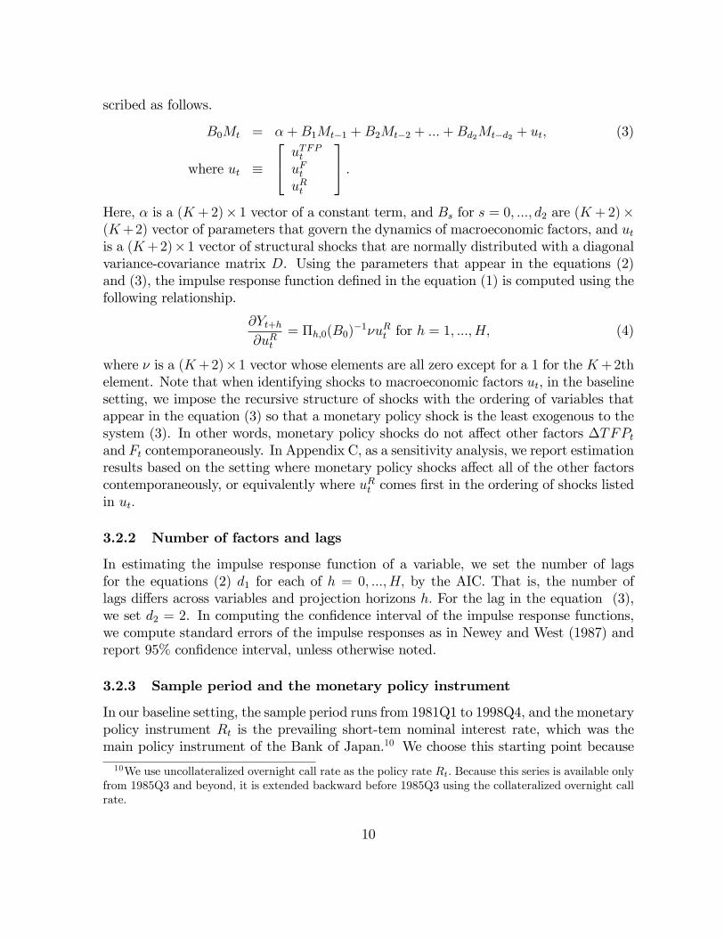
B0Mt = �+B1Mt�1 +B2Mt�2 + :::+Bd2Mt�d2 + ut; (3)

where ut �

24 uTFPt

uFtuRt

35 :Here, � is a (K +2)� 1 vector of a constant term, and Bs for s = 0; :::; d2 are (K +2)�(K+2) vector of parameters that govern the dynamics of macroeconomic factors, and utis a (K+2)�1 vector of structural shocks that are normally distributed with a diagonalvariance-covariance matrix D. Using the parameters that appear in the equations (2)and (3), the impulse response function de�ned in the equation (1) is computed using thefollowing relationship.

@Yt+h@uRt

= �h;0(B0)�1�uRt for h = 1; :::; H; (4)

where � is a (K+2)�1 vector whose elements are all zero except for a 1 for the K+2thelement. Note that when identifying shocks to macroeconomic factors ut, in the baselinesetting, we impose the recursive structure of shocks with the ordering of variables thatappear in the equation (3) so that a monetary policy shock is the least exogenous to thesystem (3). In other words, monetary policy shocks do not a¤ect other factors �TFPtand Ft contemporaneously. In Appendix C, as a sensitivity analysis, we report estimationresults based on the setting where monetary policy shocks a¤ect all of the other factorscontemporaneously, or equivalently where uRt comes �rst in the ordering of shocks listedin ut:

3.2.2 Number of factors and lags

In estimating the impulse response function of a variable, we set the number of lagsfor the equations (2) d1 for each of h = 0; :::; H; by the AIC. That is, the number oflags di¤ers across variables and projection horizons h: For the lag in the equation (3),we set d2 = 2. In computing the con�dence interval of the impulse response functions,we compute standard errors of the impulse responses as in Newey and West (1987) andreport 95% con�dence interval, unless otherwise noted.

3.2.3 Sample period and the monetary policy instrument

In our baseline setting, the sample period runs from 1981Q1 to 1998Q4, and the monetarypolicy instrument Rt is the prevailing short-tem nominal interest rate, which was themain policy instrument of the Bank of Japan.10 We choose this starting point because10We use uncollateralized overnight call rate as the policy rate Rt: Because this series is available only

from 1985Q3 and beyond, it is extended backward before 1985Q3 using the collateralized overnight callrate.

10

the micro-level data of the FIES is only available to us from 1981Q1. We choose this endpoint, taking into consideration the regime shifts in the monetary policy implementationin 1999Q1 and beyond.11 For instance, the Bank of Japan switched to pursuing a zerolower interest rate policy in 1999Q1. Within a few years, it introduced QuantitativeEasing and started to target the monetary base as well.However, we are also interested in the distributional e¤ects of monetary policy over

the entire sample period, including the period when the unconventional monetary policywas undertaken. To this end, we employ the shadow rate of the short-term nominalinterest rate in Japan estimated by Ueno (2017). The shadow rate is essentially equivalentto the prevailing short-term interest rate when it is positive, and is equivalent to whatthe short-term interest rate would be without the zero lower bound when it is negative.Shadow rates are increasingly used in studies of monetary policy implementation underthe zero lower bound. For instance, Wu and Xia (2016) construct the shadow federalfunds rate and estimate the impulse response of macroeconomic variables to a shock tothe shadow rate. Similarly to a negative shock to the federal funds rate, they �nd thata negative shock to the shadow federal funds rate leads to an increase in productionactivity and a fall in the unemployment rate. Following existing studies, including Wuand Xia (2016), we study the e¤ects of unconventional monetary policy by treating theshadow rate of the short-term interest rate as the policy rate from 1999Q1 and beyond.Admittedly, one caveat regarding the use of the shadow rate is that the rates are not

directly observable. They have to be constructed from information contained in the entireyield curve by imposing theoretical assumptions that are often di¤er across studies, andthe rates documented in existing studies, including Ueno (2017) and Krippner (2015), donot coincide with each other. Our strategy is therefore to formulate an analysis using theseries constructed by Ueno (2017) as the baseline analysis, and then conduct sensitivityanalyses using two alternative measures of the monetary policy instrument, the shadowrate constructed by Krippner (2015), and the prevailing two-year government bond yield.Figure 2 shows the time path of these rates, and the estimation results of the sensitivityanalysis are documented in Appendix C.

3.2.4 E¤ects of a monetary policy shock on macroeconomic variables

We begin by analyzing the e¤ects of a monetary policy shock on the main macroeconomicvariables estimated by the framework explained in the above section. Figure 3 shows theimpulse response function of macroeconomic variables to a negative shock, which meansan expansionary shock, to the short-term nominal interest rate, using the equation (2).For all of the panels, the point estimates of the impulse response functions based on thebaseline sample period, which runs from 1981Q1 to 1998Q4, are shown by the black linewith black circles together with dark areas that account for the 90% con�dence interval.

11Note that until 1998Q4, the Bank of Japan had continuously utilized the short-term interest ratein implementing monetary policy.

11

For the estimation results based on the sample period from 1981Q1 to 2008Q4, both thepoint estimates and con�dence interval are depicted in dotted line.The estimated response of macroeconomic variables to monetary policy shocks are

in line with existing studies such as Bernanke et al. (2005). Namely, in response to anegative shock to the short-term interest rate, quantity variables, such as GDP, invest-ment, and consumption, and price variables, such as in�ation and stock, all increase,and aggregate labor income and capital income both go up as well. Estimation resultsare qualitatively una¤ected by the choice of the sample period, though expansionarye¤ects on macroeconomic variables are less pronounced when the sample period runs upto 2008Q4.

4 E¤ects of a monetary policy shock on inequality

This section documents estimation results based on four di¤erent settings regardingthe estimation procedure: (i) The baseline estimation. This estimation uses inequalitymeasures constructed from the micro-level data set of the FIES and the sample periodcovers from 1981Q1 to 1998Q4. In other words, the estimated responses are those ofinequality measures across households whose head is employed, to shocks to the actualshort-term nominal interest rate. (ii) Estimation based on the sample period that runsfrom 1981Q1 to 2008Q4. Inequality measures are the same as the baseline estimation, butmonetary policy shocks are identi�ed as shocks to the shadow rate. (iii) Estimation thatuses what we call the adjusted Gini coe¢ cient as the earnings inequality measure. Thisadjusted Gini coe¢ cient captures earnings inequality across all households, includingthose without a working head. We do this to assess the entire impact of the job creationchannel of expansionary monetary policy shocks. (iv) Estimation that uses inequalitymeasures constructed from semi-aggregate data that runs from 2008Q4 to 2016Q2. Todo this, we use the published time series of the mean of pre-tax income of households thatbelong to �ve di¤erent groups with di¤erent income levels. We �rst construct the incomeinequality measure from this semi-aggregate data following Saiki and Frost (2014), andestimate its response to a shock to the shadow rate as well as the central bank�s balancesheet which is used as the policy instrument in Saiki and Frost (2014). Because ourmicro-level data set covers only until 2008Q4, this analysis supplements the �rst twoexercises, using the most current data.

4.1 Estimation results: baseline

Figure 4 shows the impulse response function of inequality measures of earnings yL,pre-tax income y, disposable income yD, expenditure (total consumption expenditure)cT , and consumption (non-durable consumption expenditure) cND; to a negative shock,which is an expansionary shock, to the short-term interest rate. Inequality measuresinclude variance of log, Gini coe¢ cient, and P9010. For the purpose of comparison, for

12

each of the inequality measures, we plot point estimate of the impulse response functionof earnings inequality in all of the panels in the same row.Three observations are noteworthy. First, the impact of an expansionary monetary

policy shock on income inequalities is procyclical. For instance, the variance of logof disposable income yD increases at the statistically signi�cant level of 5% for morethan three years out of �ve after the shock. The same observations hold for othertwo income variables y, and yL; and other two inequality measures. Second, such aprocyclical response arises mainly from the procyclical response of earnings yL, suggestingthe importance of the heterogenous earnings channel. This is seen from the fact that thegap of the impulse response function between earnings yL and other income variables, yand yD; is minimal, implying that the capital income and the government distributionalpolicy play a minor role in terms of the distributional consequences of monetary policyshocks. Third, the transmission of income inequality to consumption and expenditureinequality is less than one-to-one. Moreover, the responses of these inequality to shocksare often mixed in terms of the sign across time horizons following the impact period.For instance, the expenditure inequality of the variance of log reacts positively at theimpact period, but negatively at the 10-12th quarters after the impact period.

4.2 Estimation results: from 1981 to 2008

Figure 5 shows the impulse response function of the same set of inequality measures toa negative shock to the short-term interest rate extended by the shadow rate for thesample beyond 1999Q1, based on the sample period up to 2008Q4. For the purposeof comparison, in each panel, we depict by dotted lines the impulse response of theinequality measure of the same variable estimated under the baseline setting. The resultsdi¤er from those shown in Figure 4, in particular for income inequality. For almost allof the income inequality measures, the estimated impact of a monetary policy shockbecomes less pronounced.To see those changes in more detail, we study how the estimated impulse response

functions of earnings inequality vary with the sample period, by conducting rolling esti-mates of the equation (2). Figure 6 shows the results. The y-axis denotes the estimatedsize of the response to an expansionary monetary policy shock of the three inequalitymeasures that is estimated using di¤erent sample periods from 1981Q1 to an end pointthat is speci�ed on the x-axis. The size of the response is measured by the average of theimpulse response functions over 20 quarters after a shock�s impact period. Procyclicalresponses of inequality measures of earnings yL to a monetary policy shock are obtainedthroughout the 1990s. The responses, however, gradually diminish after the mid-2000sand beyond, several years after the shift of the monetary policy regime. Although notconclusive, this result suggests that a change in the response of earnings inequality to amonetary policy shock is associated with a change in economic surroundings rather thanthat in the monetary policy implementation.

13

4.3 Estimation results when changes in extensive margin ofhousehold head are counted

Inequality measures used in the analysis above are those of households whose head isemployed. The time paths of these measures therefore do not re�ect changes of inequal-ity across all households including households with a non-working head. By contrast,expansionary monetary policy shocks are expected to reduce the number of householdswhose head does not have a job and to mitigate an increase in earnings inequality arisingfrom the heterogenous earnings channel through the job creation channel. The upperpanel of Figure 7 shows the impulse response function, estimated using the equation(2), of the number of unemployed workers who are household heads, to an expansionarymonetary policy shock.12 This estimation suggests the job creation channel is at work inJapan. The number of household heads without a job, and therefore with zero earnings,declines following an accommodative monetary policy shock, possibly reducing earningsinequality across all households.In order to quantitatively assess the e¤ect arising from changes in the extensive

margin of household heads, we construct an alternative Gini coe¢ cient of earnings,which we denote as G�; that is de�ned as follows.

G� �P ~N

i=1

P ~Nj=1 jxi � xjj

2 ~NP ~N

i=1 xi= G

N~N+~N �N~N

; (5)

where

G �PN

i=1

PNj=1 jxi � xjj

2NPN

i=1 xi: (6)

Here, the equation (6) is the standard formula of the Gini coe¢ cient. In this speci�ccase, xi is earnings of the household i for i = 1; :::; N; whose head is employed. ~N is thenumber of total households including those whose head does not have a job. We assumethat earnings for those households is zero. Using the number of household heads who areemployed and the number of those who do not have a job from the aggregate statisticsnamed Labour Force Survey, for N and ~N �N; respectively, we compute an inequalitymeasure of earnings across all of the households. For G; we use the Gini coe¢ cient ofequivalized earnings.The lower panel of Figure 7 shows two impulse response functions of the adjusted

Gini coe¢ cient of earnings G� to an expansionary shock to a monetary policy, based on12In estimating responses in Figure 7, we use the number of unemployed household heads, including

those aged 60 and higher and 24 and younger, in the Labour Force Survey published by the Ministryof Internal A¤airs and Communications. Ideally, we should use the subset of those households aged25-59 so as to maintain consistency of population of households based on which the inequality measuresstudied in the rest of the paper are constructed. Such a series is, however, not available in the survey.Similarly, the number of employed household heads is also not available.

14

sample periods that run up to 1998Q4 and up to 2008Q4, respectively. The distributionale¤ects of a monetary policy shock are insigni�cant even in the former sample period.Admittedly, some caveats apply to our adjusted Gini coe¢ cient G�; as a measure of

income inequality. This measure, for instance, does not capture changes in income dis-tribution arising from capital income and the government transfer.13 However, the resultof this exercise, combined with the estimated response functions of unemployed house-hold heads, suggests the possibility that a decline in earnings inequality due to the jobcreation channel counters a rise in earnings inequality stemming from the heterogenousearnings channel after an expansionary monetary policy shock.

4.4 Estimation results: from 2008 to 2016

The limitation of the estimation exercises above is that these are based on the sampleperiod before 2009, due to the unavailability of the micro-level data of the FIES. In or-der to study whether the distributional e¤ects of a monetary policy shock have recentlychanged, we follow Saiki and Frost (2014) and construct an alternative inequality mea-sure of pre-tax income y from the semi-aggregate income series of households includedin the FIES. The FIES publishes time series of pre-tax income y of households, includ-ing those whose head is not employed, by �ve di¤erent income quantiles from January2002 to the present. We use as our pre-tax income inequality measure the di¤erence ofaveraged income y of households of the highest income quantile, the 80�100th, and thatof the lowest income quantile, the 0�20th, and estimate the response of the measure to amonetary policy shock. It is notable, however, that, although this analysis delivers usefulinformation regarding the most recent relationship between monetary policy shocks andinequality measures, there are some limitations as well. First, we are only able to studypre-tax income y, since the FIES does not publish other income and consumption seriesby households�income levels. Second, this pre-tax income inequality measure does notcapture changes in inequality within each of the two di¤erent income groups. Lastly,the population of sampled households in this measure does not accord precisely with thescope of households speci�ed in Section 3.1.2.To check robustness, in estimating the impulse response functions of the pre-tax

income inequality measures to a monetary policy shock, we formulate two separate exer-cises using di¤erent estimation procedures; the VAR used in Saiki and Frost (2014), andthe LLP based on the equation (2). The VAR in Saiki and Frost (2014) consists of �vevariables, including real GDP, in�ation, assets held by the Bank of Japan, stock prices,and the pre-tax income inequality measure. A monetary policy shock is identi�ed as ashock to the assets held by the Bank of Japan by the Cholesky decomposition with thisordering of the variables.14 In both estimations, the sample period runs from 2008Q4 to

13In addition, because the relevant data are not available, we use the number of household heads ofall ages instead of those aged from 25�59.14To consider the e¤ects of the Great East Japan earthquake of March 11th, 2011 in Japan, following

15

2016Q2.Figure 8 shows the impulse response function of pre-tax income inequality to a shock

to the measure of the monetary policy adopted in Saiki and Frost (2014) in the upperpanel, and that to a shock to the shadow rate of Ueno (2017) in the lower panel. Thoughpoint estimates are positive and in line with what Saiki and Frost (2014) document, bothestimation results agree that responses of pre-tax income inequality to a monetary policyshock are not statistically signi�cant. This result therefore con�rms that estimationresults obtained in Figure 5 are robust to the extension of the data sample.15

5 Accounting for estimation results

Why did the once-prevailing distributional e¤ects of monetary policy diminish during the2000s? And why didn�t consumption inequality increase as much as income inequalityin the period before the 2000s? What role did �nancial assets and liabilities play in thedistributional e¤ects of monetary transmission?To address to these questions, we employ three toolkits. The �rst one is a New

Keynesian Dynamic Stochastic General Equilibrium (DSGE) model that consists of twoproduction sectors and two types of representative households. The DSGE model is usedto illustrate how the distributional e¤ects of a monetary policy shock change with thestructure of the economy in a way we observed in the empirical exercises above, ratherthan providing a quantitative model that closely matches with all of our empirical ob-servations. From this view point, our model is absent from some of the channels, suchas the job creation channel and the income composition channel, since, as indicated byFigure 4 and 5, the heterogenous earnings channel appears as the central to the distri-butional e¤ects of monetary policy in Japan. We discuss, based on the model, that twoelements, the labor market �exibility and the distribution of households��nancial assetsand liabilities, have potential to shape responses of income and consumption inequalityto monetary policy shocks in an important manner. The other two toolkits include twotypes of alternative data set, industry-level aggregate data sets that contain time seriesof labor market variables and goods production, and the micro-level data of a house-hold�s �nancial assets and liabilities. These data sets complement the data collected inthe FIES. We use those data sets as well as inequality measures constructed from theFIES to check whether the model�s predictions accord with the data.

Saiki and Frost (2014), we introduce two exogenous dummy variables, which they call �earthquake�and�earthquake response�in their paper. Each of the two dummy variables takes unity for the period from2011Q2 to 2011Q3, and from 2011Q4 to 2012Q1, and takes zero if otherwise, respectively.15Note that Saiki and Frost (2014) show that an expansionary shock to their monetary policy measure

leads to an increase in the pre-tax income inequality measure in a statistically signi�cant manner whenthe sample period runs from 2008Q4 to 2014Q1.

16

5.1 A model with two types of representative households

5.1.1 Setting

Two householdsThere are two types of an in�nitely-lived representative household, X and Z; each of

which has two types of members; one member that supplies its labor inputs to one of thetwo sectors exclusively, and another member that can split its labor inputs, supplyingits labor inputs to both sectors. We refer to these as attached and mobile labor inputs,respectively. Households receive utility from consumption Ct; and disutility from workinghours of the �rst type of member denoted as Nt; and those of the second type of memberdenoted as Ht: The expected utility function (7) is described in the following manner.

Us;t � Et

" 1Xq=0

�q

log (Cs;t+q � bCs;t+q�1)� �

N1+�s;t+q

1 + �� �

H1+�s;t+q

1 + �

!#; (7)

for s = X and Z: Here, � 2 (0; 1) is the discount factor, b > 0 captures the degree ofhabit formation, �; � > 0 are the inverse of the Frisch labor-supply elasticity, and � and� > 0 are the weighting assigned to attached and mobile labor inputs, respectively:The budget constraint for each of the households is given by

Cs;t +Bs;tPt

�

2666664Ws;t

PtNs;t +

Wt

PtHs;t

+��X;t+�Z;t

Pt

� �;s

+�RX;tKX+RZ;tKZ

Pt

� K;s

+Rt�1Bs;t�1Pt

+ �B

�Bs;tPt

�2

3777775 ; for s = X and Z; (8)

where Pt is the aggregate price index that corresponds to the consumption composite,Bs;t is the nominal bond holding, and Ws;t and Wt are the nominal wages paid to theattached labor inputs of the household s; for s = X and Z; and the mobile labor inputs,respectively. Notice that the nominal wage for attached labor inputs Ws;t di¤ers acrosshousehold types, and that of mobile labor inputs Wt is common across household types.�X;t + �Z;t is the nominal dividend from the two sectors; �;s 2 [0; 1] is the share ofdividends held by the household s; RX;t and RZ;t are the nominal rental costs of thecapital stock used in the two sectors, KX and KZ ; K;s 2 [0; 1] is the share of capitalstock held by the household s; Rt�1 is the nominal return to bonds holding; and �B > 0is the parameter that governs the adjustment costs of bond holding. For simplicity, weassume that the shares of dividend and capital income are not tradable and constantover time.

Firms�goods productionThe economy consists of two sectors, X and Z; and each sector has �nal goods �rms

and a continuum of intermediate goods �rms. Perfectly competitive �nal goods �rms

17

use a continuum of intermediate goods i 2 (0; 1) for the sector X and j 2 (0; 1) for thesector Z; and produce the gross output ~Xt and ~Zt that are used for constructing theconsumption basket Ct. The gross output are produced using the following productiontechnology;

~Xt =

�Z 1

0

xt (i)1�"�1 di

� ""�1

and ~Zt =�Z 1

0

zt (j)1�"�1 dj

� ""�1

;

where " 2 (1;1) denotes the elasticity of substitution between di¤erentiated productsand xt (i) and zt (j) are products of intermediate goods �rms in the two sectors.The demand functions for the di¤erentiated products produced by �rm i and j are

derived from the optimization behavior of the �nal goods �rms, and they are representedby

xt (i) =

�PX;t (i)

PX;t

��"~Xt and zt (j) =

�PZ;t (j)

PZ;t

��"~Zt; (9)

where fPX;t (i)g and fPZ;t (j)g for i; j 2 [0; 1] are the nominal price of the di¤erentiatedproducts, and PX;t and PZ;t are the price indices of the two �nal goods that are expressedas

PX;t =

�Z 1

0

PX;t (i)1�" di

� 11�"

and PZ;t =�Z 1

0

PZ;t (j)1�" dj

� 11�"

:

Each intermediate goods �rm produces goods from two types of labor inputs and thesector-speci�c capital stock, with the Cobb-Douglas production technology describedbelow.

xt (i) = ANX;t (i)�� UX;t (i)

�(1��)KX;t (i)1�� ; and (10)

zt (j) = ANZ;t (j)�� UZ;t (j)

�(1��)KZ;t (j)1�� : (11)

Here, A is the technology level that is common to the two sectors; NX;t (i) and NZ;t (j) ;UX;t (i) and UZ;t (j) ; and KX;t (i) and KZ;t (j) ; are the attached labor inputs, mobilelabor inputs, and sector speci�c capital inputs used by the �rm i and j; and � and� 2 [0; 1] are the parameters that govern the production technology.

Firms�price settingDi¤erentiated �rms i and j are monopolistic competitors in the products market. A

�rm i in the sector X sets the price for its products PX;t (i) in reference to the demandgiven by the equation (9) : It can reset the prices solving the following problem:

18

maxPX;t(i)

Et

" 1Xq=0

�t+q�t+q�t

�t+q;X (i)

Pt+q

#(12)

s:t: �t+q;X (i) = PX;t+q (i)xt+q (i)�MCX;t+q (i)xt+q (i)��X2

�PX;t+q (i)

PX;t+q�1 (i)� 1�2PX;t+qXt+q;

(13)where �t+q is the Lagrange multiplier associated with budget constraint (8) of the house-hold in the period t + q; MCX;t+q (i) is the nominal marginal cost derived from theproduction function (10) ; that is given as follows.

MCX;t =��MCW

��X;tW

�(1��)t R1��X;t

A;where ��MC � (��)

��� (� (1� �))��(1��) (1� �)��1 :(14)

�X > 0 is the parameter associated with price adjustment. A �rm j faces a similarproblem with the parameter �Z > 0: Note that we assume the symmetric equilibriumwhere all of the di¤erentiated goods prices PX;t+q (i) and PZ;t+q (j) set by intermediategoods �rms are identical, so that PX;t+q (i) = PX;t+q and PZ;t+q (j) = PZ;t+q:

AggregationThere are agents named aggregators that purchase each of the value-added of two

goods, which we denote as Xt and Zt and de�ned below, and construct the compositeof consumption goods from the two goods, using the following technology, and sell thegoods to households in a competitive manner.

Ct = X�t Z

1��t ; (15)

where � 2 [0; 1] is the technology parameter associated with the aggregation. Notethat the cost minimization problem of aggregators given the aggregation technology (15)implies that the aggregate price index is expressed as

Pt = ��� (1� �)��1 P �X;tP

1��Z;t : (16)

Note also that using this price index, the demand for each of the two goods can beshown as follows.

Xt = �

�PtPX;t

�Ct and Zt = (1� �)

�PtPZ;t

�Ct: (17)

The government

19

The central bank adjusts the nominal interest rate so as to stabilize the growth ratesof the price index Pt.

logRt = �n logRt�1 + (1� �n)' log �t + �R;t; (18)

where �t is Pt=Pt�1, and �n 2 [0; 1) and ' > 0 are the parameters and �R;t is an innovationto the monetary policy rule.

Resource constraintThe resource constraints for three production inputs are given as follows.

Z 1

0

NX;t (i) di = NX;t andZ 1

0

NZ;t (j) dj = NZ;t; (19)Z 1

0

UX;t (i) di+

Z 1

0

UZ;t (j) dj = HX;t +HZ;t; (20)Z 1

0

KX;t (i) di = KX andZ 1

0

KZ;t (j) dj = KZ: (21)

Note that two terms in the left hand side of the equation (20) stands for the amountof labor inputs by mobile workers to sector X and Z; while those in the right handside of the equation stands for the amount of labor input supplied by mobile workers inhousehold X and Z:We hereafter denote the total labor inputs of mobile workers in thetwo sectors by UX;t and UZ;t.The resource constraints for the gross output produced by �nal goods producers ~Xt

and ~Zt are given as follows.

~Xt = Xt +�X2

�PX;tPX;t�1

� 1�2Xt and

~Zt = Zt +�Z2

�PZ;tPZ;t�1

� 1�2Zt:

For the consumption composite, the sum of consumption of the two representativehouseholds equals the total amount of consumption composite produced by the aggre-gators, less costs associated with nominal bond holding paid by the two households.

CX;t + CZ;t = Ct � �B�BX;tPt

�2� �B

�BZ;tPt

�2:

Finally, the total supply of the nominal bond in the aggregate is assumed to be zero.

BX;t +BZ;t = 0:

20

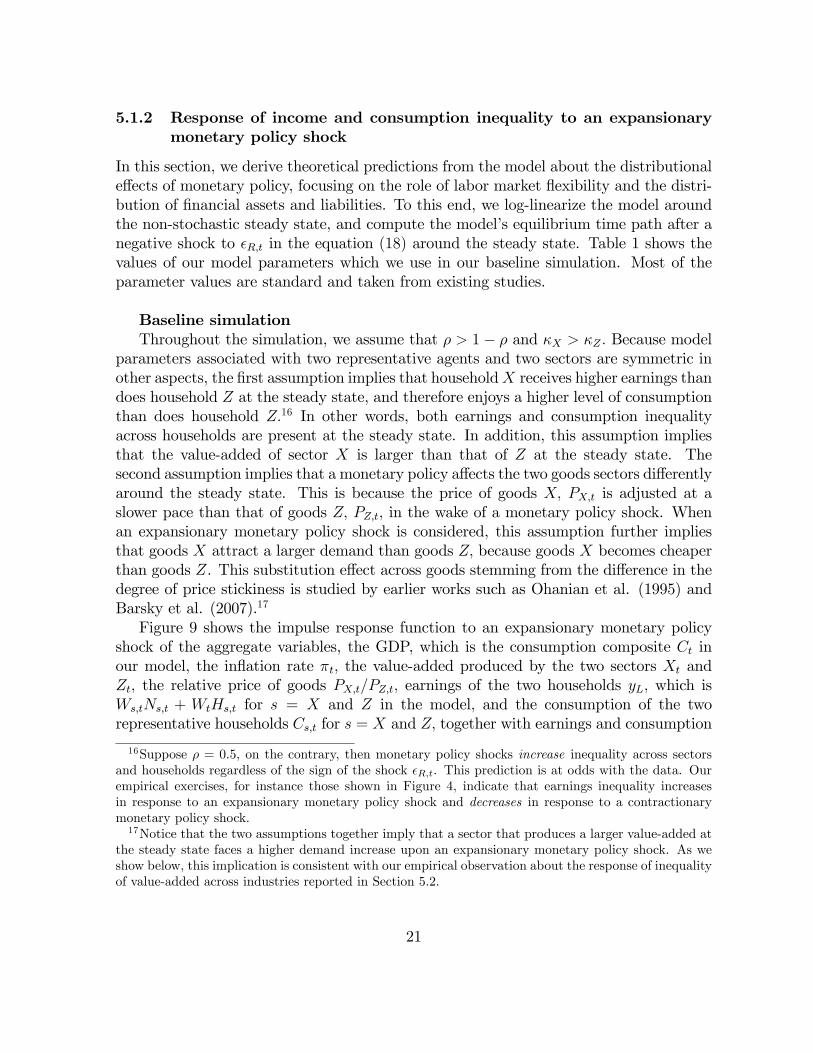
5.1.2 Response of income and consumption inequality to an expansionarymonetary policy shock

In this section, we derive theoretical predictions from the model about the distributionale¤ects of monetary policy, focusing on the role of labor market �exibility and the distri-bution of �nancial assets and liabilities. To this end, we log-linearize the model aroundthe non-stochastic steady state, and compute the model�s equilibrium time path after anegative shock to �R;t in the equation (18) around the steady state. Table 1 shows thevalues of our model parameters which we use in our baseline simulation. Most of theparameter values are standard and taken from existing studies.

Baseline simulationThroughout the simulation, we assume that � > 1� � and �X > �Z : Because model

parameters associated with two representative agents and two sectors are symmetric inother aspects, the �rst assumption implies that householdX receives higher earnings thandoes household Z at the steady state, and therefore enjoys a higher level of consumptionthan does household Z:16 In other words, both earnings and consumption inequalityacross households are present at the steady state. In addition, this assumption impliesthat the value-added of sector X is larger than that of Z at the steady state. Thesecond assumption implies that a monetary policy a¤ects the two goods sectors di¤erentlyaround the steady state. This is because the price of goods X; PX;t is adjusted at aslower pace than that of goods Z; PZ;t; in the wake of a monetary policy shock. Whenan expansionary monetary policy shock is considered, this assumption further impliesthat goods X attract a larger demand than goods Z; because goods X becomes cheaperthan goods Z. This substitution e¤ect across goods stemming from the di¤erence in thedegree of price stickiness is studied by earlier works such as Ohanian et al. (1995) andBarsky et al. (2007).17

Figure 9 shows the impulse response function to an expansionary monetary policyshock of the aggregate variables, the GDP, which is the consumption composite Ct inour model; the in�ation rate �t; the value-added produced by the two sectors Xt andZt; the relative price of goods PX;t=PZ;t; earnings of the two households yL; which isWs;tNs;t + WtHs;t for s = X and Z in the model; and the consumption of the tworepresentative households Cs;t for s = X and Z; together with earnings and consumption

16Suppose � = 0:5, on the contrary, then monetary policy shocks increase inequality across sectorsand households regardless of the sign of the shock �R;t. This prediction is at odds with the data. Ourempirical exercises, for instance those shown in Figure 4, indicate that earnings inequality increasesin response to an expansionary monetary policy shock and decreases in response to a contractionarymonetary policy shock.17Notice that the two assumptions together imply that a sector that produces a larger value-added at

the steady state faces a higher demand increase upon an expansionary monetary policy shock. As weshow below, this implication is consistent with our empirical observation about the response of inequalityof value-added across industries reported in Section 5.2.

21

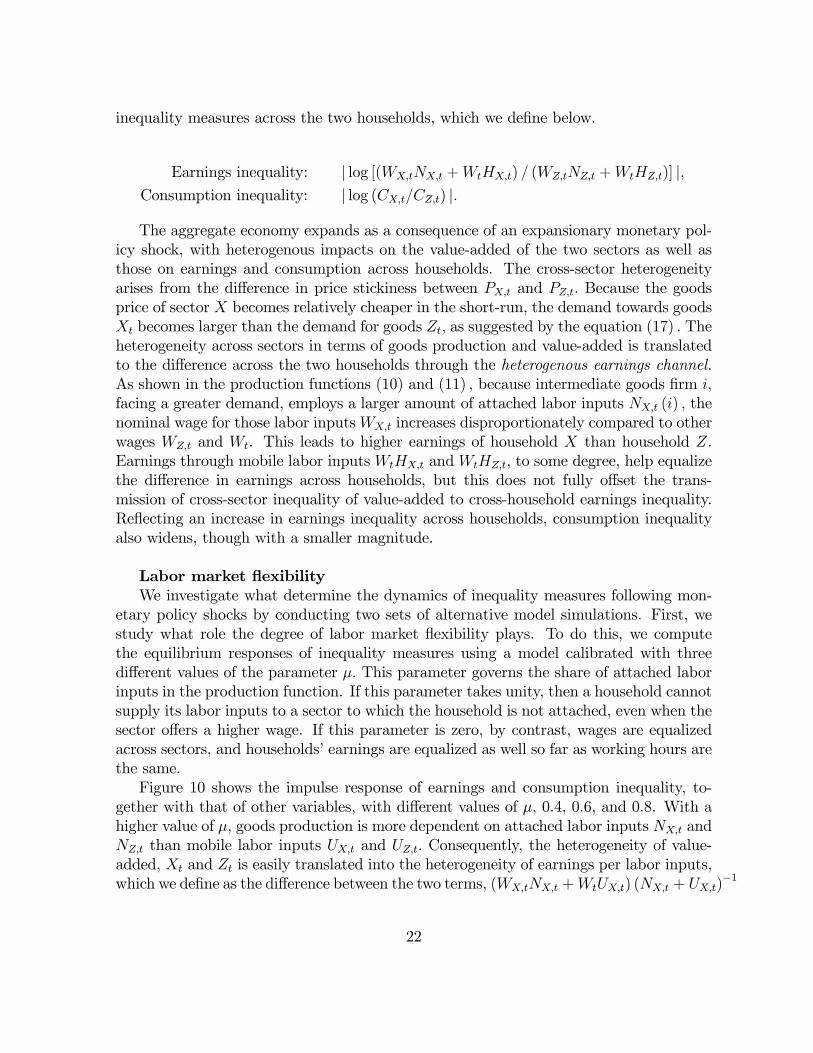
inequality measures across the two households, which we de�ne below.

Earnings inequality: j log [(WX;tNX;t +WtHX;t) = (WZ;tNZ;t +WtHZ;t)] j;Consumption inequality: j log (CX;t=CZ;t) j:

The aggregate economy expands as a consequence of an expansionary monetary pol-icy shock, with heterogenous impacts on the value-added of the two sectors as well asthose on earnings and consumption across households. The cross-sector heterogeneityarises from the di¤erence in price stickiness between PX;t and PZ;t: Because the goodsprice of sector X becomes relatively cheaper in the short-run; the demand towards goodsXt becomes larger than the demand for goods Zt; as suggested by the equation (17) : Theheterogeneity across sectors in terms of goods production and value-added is translatedto the di¤erence across the two households through the heterogenous earnings channel.As shown in the production functions (10) and (11) ; because intermediate goods �rm i;facing a greater demand, employs a larger amount of attached labor inputs NX;t (i) ; thenominal wage for those labor inputsWX;t increases disproportionately compared to otherwages WZ;t and Wt. This leads to higher earnings of household X than household Z.Earnings through mobile labor inputs WtHX;t and WtHZ;t; to some degree, help equalizethe di¤erence in earnings across households, but this does not fully o¤set the trans-mission of cross-sector inequality of value-added to cross-household earnings inequality.Re�ecting an increase in earnings inequality across households, consumption inequalityalso widens, though with a smaller magnitude.

Labor market �exibilityWe investigate what determine the dynamics of inequality measures following mon-

etary policy shocks by conducting two sets of alternative model simulations. First, westudy what role the degree of labor market �exibility plays. To do this, we computethe equilibrium responses of inequality measures using a model calibrated with threedi¤erent values of the parameter �: This parameter governs the share of attached laborinputs in the production function. If this parameter takes unity, then a household cannotsupply its labor inputs to a sector to which the household is not attached, even when thesector o¤ers a higher wage. If this parameter is zero, by contrast, wages are equalizedacross sectors, and households�earnings are equalized as well so far as working hours arethe same.Figure 10 shows the impulse response of earnings and consumption inequality, to-

gether with that of other variables, with di¤erent values of �; 0.4, 0.6, and 0.8. With ahigher value of �; goods production is more dependent on attached labor inputs NX;t andNZ;t than mobile labor inputs UX;t and UZ;t: Consequently, the heterogeneity of value-added, Xt and Zt is easily translated into the heterogeneity of earnings per labor inputs,which we de�ne as the di¤erence between the two terms, (WX;tNX;t +WtUX;t) (NX;t + UX;t)

�1

22

and (WZ;tNZ;t +WtUZ;t) (NZ;t + UZ;t)�1 ; since the production share of attached labor in-

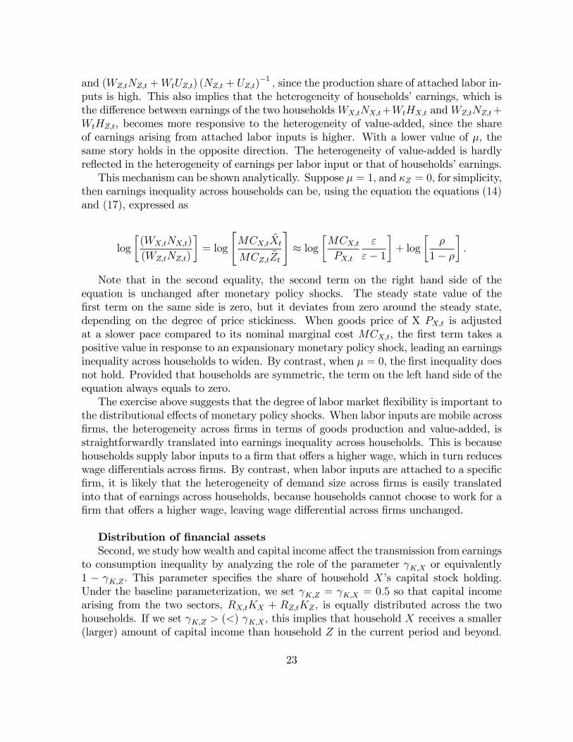
puts is high. This also implies that the heterogeneity of households�earnings, which isthe di¤erence between earnings of the two householdsWX;tNX;t+WtHX;t andWZ;tNZ;t+WtHZ;t, becomes more responsive to the heterogeneity of value-added, since the shareof earnings arising from attached labor inputs is higher. With a lower value of �; thesame story holds in the opposite direction. The heterogeneity of value-added is hardlyre�ected in the heterogeneity of earnings per labor input or that of households�earnings.This mechanism can be shown analytically. Suppose � = 1; and �Z = 0; for simplicity,

then earnings inequality across households can be, using the equation the equations (14)and (17), expressed as

log

�(WX;tNX;t)

(WZ;tNZ;t)

�= log

"MCX;t ~Xt

MCZ;t ~Zt

#� log

�MCX;tPX;t

"

"� 1

�+ log

��

1� �

�:

Note that in the second equality, the second term on the right hand side of theequation is unchanged after monetary policy shocks. The steady state value of the�rst term on the same side is zero, but it deviates from zero around the steady state,depending on the degree of price stickiness. When goods price of X PX;t is adjustedat a slower pace compared to its nominal marginal cost MCX;t, the �rst term takes apositive value in response to an expansionary monetary policy shock, leading an earningsinequality across households to widen. By contrast, when � = 0; the �rst inequality doesnot hold. Provided that households are symmetric, the term on the left hand side of theequation always equals to zero.The exercise above suggests that the degree of labor market �exibility is important to

the distributional e¤ects of monetary policy shocks. When labor inputs are mobile across�rms, the heterogeneity across �rms in terms of goods production and value-added, isstraightforwardly translated into earnings inequality across households. This is becausehouseholds supply labor inputs to a �rm that o¤ers a higher wage, which in turn reduceswage di¤erentials across �rms. By contrast, when labor inputs are attached to a speci�c�rm, it is likely that the heterogeneity of demand size across �rms is easily translatedinto that of earnings across households, because households cannot choose to work for a�rm that o¤ers a higher wage, leaving wage di¤erential across �rms unchanged.

Distribution of �nancial assetsSecond, we study how wealth and capital income a¤ect the transmission from earnings

to consumption inequality by analyzing the role of the parameter K;X or equivalently1 � K;Z : This parameter speci�es the share of household X�s capital stock holding.Under the baseline parameterization, we set K;Z = K;X = 0:5 so that capital incomearising from the two sectors, RX;tKX + RZ;tKZ ; is equally distributed across the twohouseholds. If we set K;Z > (<) K;X ; this implies that household X receives a smaller(larger) amount of capital income than household Z in the current period and beyond:

23

Because a household determines its time path of consumption with reference to its totalincome stream, a change in the share of capital stock holding should lead to a change inthe dynamics of consumption inequality following monetary policy shocks.Figure 11 shows impulse response functions of earnings and consumption inequality,

again together with other relevant variables, with di¤erent values for K;X ; 0:4; 0:5; and0:6: The distribution of capital stock holding substantially a¤ects the dynamics of bothearnings and consumption inequality following monetary policy shocks. With a smallershare of capital stock holding K;X , household X becomes less wealthy and thereforesupplies more labor inputs to the goods producing sectors due to the negative wealthe¤ect. By contrast, household Z; with a larger share of capital stock holding K;Z ;works less, further boosting earnings inequality across households. These changes in theresponse of labor inputs are, however, not su¢ ciently sizable to overturn the e¤ects onconsumption inequality arising from the di¤erence in the present and future stream ofcapital income. Household Z consumes a greater amount of goods, as it now receivesa larger share of capital income today and future, and household X consumes less.Consequently, the dispersion of consumption level across households is reduced.The exercise suggests that the distribution of �nancial assets and liabilities has the

potential to mitigate the translation of earnings inequality to consumption inequality.For instance, suppose a household that confronts a larger increase in earnings has a feweramount of �nancial assets. A change in consumption inequality across households thenshould become minor compared with a change in earnings inequality. Using alternativedata sources, we explore below whether the distributions of Japanese households�assetsand liabilities are consistent with this prediction.

5.2 Monetary policy shocks and earnings inequality

Provided that the cross-�rm or cross-industry heterogeneity of monetary policy e¤ectsare present, our theoretical model predicts that whether or not they result in earningsinequality across households depends on the degree of labor market �exibility. In thissection, using the industry-level data sets of labor market and �rm variables, we showthat the data are in fact consistent with this prediction.We start by brie�y describing the nature of labor markets in Japan and their develop-

ments. Existing studies agree that a low �exibility of labor inputs adjustments throughthe extensive margins (adjustments with heads) has been a notable feature that charac-terizes Japanese labor markets. For instance, Braun et al. (2006) examine business cyclecharacteristics of labor market variables for the U.S. and Japan over the period from1960 to 2002. They show that in Japan, variations in the extensive margin are about60% of those of the intensive margin (hours of work per employee), whereas the numberis 245% in the U.S. They then argue that in Japan labor inputs adjustments by a �rmare made through working hours of existing workers, rather than through the hiring or�ring of workers.

24

Since around the mid-1990s, however, labor markets in Japan has gone through im-portant changes gradually. First, temporary workers have started to play a larger rolein labor markets. Unlike regular workers, the period of employment for these workers istypically �xed, and limited to a short period of time, allowing �rms to arrange more �ex-ible labor inputs adjustments through the extensive margin. The upper panel of Figure12 shows the time path of the proportion of employees who work as temporary workersover the total number of employees. The proportion exhibits a secular increase over theyears, indicating that �rms are becoming less dependent on adjustments through theintensive margin, and more dependent on adjustments through the extensive margin. Inaddition, partly due to an increase in temporary workers, there has been an enhance-ment in the degree of labor market mobility. The lower panel of Figure 12 shows thetime path of labor turnover ratio, which indicates that workers tend recently to be more�exible in switching to jobs that o¤er a more favorable term, compared to the old days.These changes suggest that the degree of labor market �exibility, that was once low, hasbeen changed such that the cross-�rm or cross-industry heterogeneity of value-added isless likely to be translated into the heterogeneity of earnings per employee and earningsper labor input. This is because workers supply labor inputs to a �rm that pays higheruntil earnings di¤erential diminishes. Consequently, the cross-�rm heterogeneity is nolonger translated into earnings inequality across households. In the next subsection, weempirically show that this is indeed the case.

5.2.1 Responses of inequality measures across industries

Because the FIES does not collect detailed data of �rms and workers in which we areinterested, we conduct additional exercises using the industry-level data sets that con-tain such information, and study how the cross-industry heterogeneity of value-added istranslated to that of earnings per employee and that of earnings per labor input. Forthis purpose, we construct an inequality measure across industries of the value-addedand earnings per employee from the corresponding data of industry groups in the Finan-cial Statements Statistics of Corporations (FSSC) published by the Ministry of Finance.The FSSC reports the data of 37 industries and each industry consists of four groupscategorized by the size of capital. We therefore construct inequality measures across 37� 4 industry groups of the FSSC.18 We also construct inequality measures across indus-tries of earnings per working hours from the corresponding data of 35 industries in theMonthly Labour Survey (MLS) by the Ministry of Health, Labour and Welfare.19 Wethen estimate the response of these inequality measures to an expansionary shock to theshort-term interest rate Rt, using the LLP speci�ed in the equation (2).

18The FSSC reports the data series by size of capital: (1) less than 50 million yen, (2) 50 million yento 100 million yen, (3) 100 million yen to 1 billion yen, (4) more than 1 billion yen.19The earnings per employee is calculated by dividing �Salaries and wages�of an industry group by

�Number of employees�of the same group reported in FSSC. The earnings per working hour is calculatedby dividing �Total cash earnings�per employee by �Total hours worked�per employee reported in MLS.

25

The left panels of Figure 13 show the results of the estimation based on the sampleperiod running from 1981Q1 to 1998Q4. An expansionary monetary policy shock leads toa rise in inequality across industries in terms of value-added, earnings per employee, andearnings per working hours. Apparently, the cross-industry heterogeneity of value-addedis translated into that of earnings per employee and per working hours. In order to seethe e¤ects of higher labor market �exibility, we estimate the response of these inequalitymeasures to a monetary policy shock, now using the sample period from 1981Q1 to2008Q4, which includes a period when labor market �exibility was already high. Theright panels of Figure 13 show the estimation results. The procyclical responses ofinequality in terms of value-added is still observed in this setting. In contrast to theresults documented in the left panel of the �gure, however, this response of inequalityis not translated into inequality in terms of earnings per employee and of earnings perworking hour. This weakening of translation of inequality from value-added to earningsaccords well with the model�s prediction shown in Figure 9 and 10, and supports theview that a change in labor market �exibility alters responses of earnings inequality toa monetary policy shock.20

5.3 Transmission of income inequality to consumption inequal-ity and the role of �nancial assets

5.3.1 Responses of the MPC by household�s income quantiles

As Figure 4 shows, we �nd that the transmission of monetary policy shocks to con-sumption inequality is slightly procyclical or insigni�cant, even when earnings inequalityexhibits a signi�cant procyclical response to these shocks. In this section, we explore thereasons for this. We �rst show that the response of consumption inequality is insignif-icant, not because the responses of �mean�of consumption of households are all weak,but because the response of �mean�of consumption of low-income households is substan-tially large compared with that of high-income households. We then ask if households��nancial positions are responsible for these observations, using the micro-level data of�nancial positions.To this end, we divide the households surveyed in the FIES into �ve subgroups

depending on their income quantiles, and construct time series of the mean of disposableincome yD and consumption cND of households in each group. We then compute theresponse of the mean of the two series yD and cND to an expansionary monetary policyshock, using the estimation equation (2) for these �ve groups. In addition, we computea measure of the MPC by subtracting the response of disposable income yD from thatof consumption cND:

20For the sensitivity analysis, we conduct the same estimation exercise using inequality measuresacross 37 industries using the data of the FSSC for the sample period from 1981Q1 to 1998Q4 and thatfrom 1981Q1 to 2008Q4. The results are qualitatively the same as those shown in Figure 13.

26

Figure 14 shows the response of mean of consumption cND and MPC, following amonetary policy shock, for households that fall in the 80�100% income quantile andthose that fall in the 0�20% income quantile in the upper and lower panel, respectively.Consumption responses to a monetary policy shock are positive for both groups of house-holds and comparable across these groups. MPC conditional on monetary policy shocksis greater for households of a low-income quantile compared with those of a high-incomequantile. It appears that the greater response of MPC in low-income households is acause of the moderate translation of earnings inequality to consumption inequality.

5.3.2 Distributional e¤ects via �nancial asset holdings

Why is the MPC conditional on monetary policy shocks higher for households in the lowincome quantile? We consider two possible explanations. The �rst explanation rests onthe distribution of �nancial assets and liabilities across households at the time of arrivalof a monetary policy shock. Our simulation exercise in Figure 11 shows the distribu-tion is relevant to the response of consumption inequality to a monetary policy shock.The cyclical response of consumption inequality is attenuated when household Z holds agreater share of �nancial assets. Existing empirical studies, such as Doepke and Schnei-der (2006), Domanski et al. (2016), and O�Farrell et al. (2016), also underscore theimportance of the heterogeneity of households��nancial positions on the distributionale¤ects of monetary policy, as the heterogeneity of the distributions acts as a source ofthe portfolio channel and the savings distribution channel.21 The second explanation is adi¤erence in consumption behavior across households with di¤erent income level. If theMPC is higher by nature for low-income households for any reason, then it can serve asan explanation for the minor response of consumption inequality. For instance, Jappelliand Pistaferri (2014) argue that if households falling in a lower income quantile are moreliquidity-constrained than those in a higher income quantile, the MPC of those house-holds tends to be higher. Also, Carroll and Kimball (1996) discuss that a precautionalmotive explains the higher MPC for the poor and lower MPC for the rich.Our strategy is to exploit micro-level data of households��nancial positions collected

in the Survey of Household Finances (SHF), and examine if these are distributed in away that is consistent with the MPC of low-income households being higher than thatof high-income households, so that the response of consumption inequality is mitigated

21Our discussion here is not inconsistent with our empirical observation that the most of cyclicaldynamics of income inequality is attributed to those of earnings inequality shown in Figure 4. It isnotable that the FIES does not count the capital gains or losses as a part of capital income. Evenwhen there is a rise in the value of a household�s asset due to monetary expansion and the householdincreases its consumption accordingly through the portfolio channel, so far as the household does notsell the asset, other things being equal, it leads to an increase in its MPC. Similarly, the FIES does notcount a change in the real value of household�s debt possibly by changes in in�ation rate as a change inincome as well. If the household increases its consumption as a result through the savings distributionchannel, it observationally results in an increase in its MPC.

27

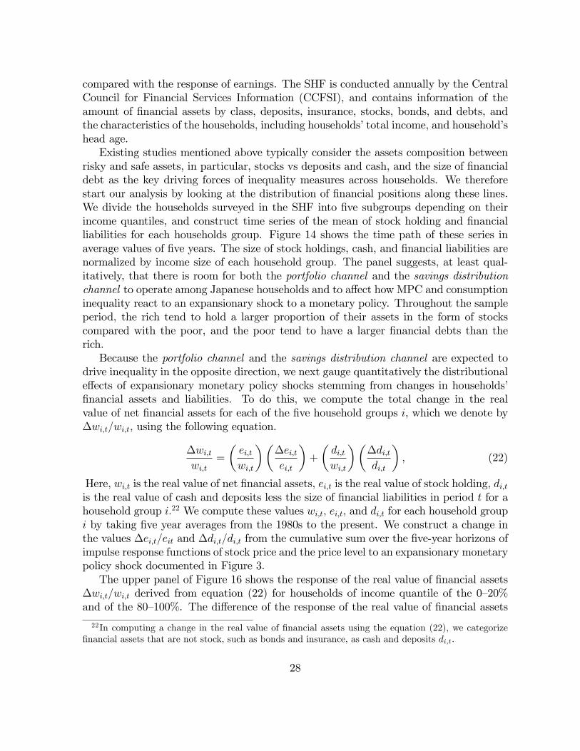
compared with the response of earnings. The SHF is conducted annually by the CentralCouncil for Financial Services Information (CCFSI), and contains information of theamount of �nancial assets by class, deposits, insurance, stocks, bonds, and debts, andthe characteristics of the households, including households�total income, and household�shead age.Existing studies mentioned above typically consider the assets composition between

risky and safe assets, in particular, stocks vs deposits and cash, and the size of �nancialdebt as the key driving forces of inequality measures across households. We thereforestart our analysis by looking at the distribution of �nancial positions along these lines.We divide the households surveyed in the SHF into �ve subgroups depending on theirincome quantiles, and construct time series of the mean of stock holding and �nancialliabilities for each households group. Figure 14 shows the time path of these series inaverage values of �ve years. The size of stock holdings, cash, and �nancial liabilities arenormalized by income size of each household group. The panel suggests, at least qual-itatively, that there is room for both the portfolio channel and the savings distributionchannel to operate among Japanese households and to a¤ect how MPC and consumptioninequality react to an expansionary shock to a monetary policy. Throughout the sampleperiod, the rich tend to hold a larger proportion of their assets in the form of stockscompared with the poor, and the poor tend to have a larger �nancial debts than therich.Because the portfolio channel and the savings distribution channel are expected to

drive inequality in the opposite direction, we next gauge quantitatively the distributionale¤ects of expansionary monetary policy shocks stemming from changes in households��nancial assets and liabilities. To do this, we compute the total change in the realvalue of net �nancial assets for each of the �ve household groups i, which we denote by�wi;t=wi;t; using the following equation.

�wi;twi;t

=

�ei;twi;t

���ei;tei;t

�+

�di;twi;t

���di;tdi;t

�; (22)

Here, wi;t is the real value of net �nancial assets, ei;t is the real value of stock holding, di;tis the real value of cash and deposits less the size of �nancial liabilities in period t for ahousehold group i:22 We compute these values wi;t; ei;t, and di;t for each household groupi by taking �ve year averages from the 1980s to the present. We construct a change inthe values �ei;t=eit and �di;t=di;t from the cumulative sum over the �ve-year horizons ofimpulse response functions of stock price and the price level to an expansionary monetarypolicy shock documented in Figure 3.The upper panel of Figure 16 shows the response of the real value of �nancial assets

�wi;t=wi;t derived from equation (22) for households of income quantile of the 0�20%and of the 80�100%. The di¤erence of the response of the real value of �nancial assets

22In computing a change in the real value of �nancial assets using the equation (22), we categorize�nancial assets that are not stock, such as bonds and insurance, as cash and deposits di;t:

28

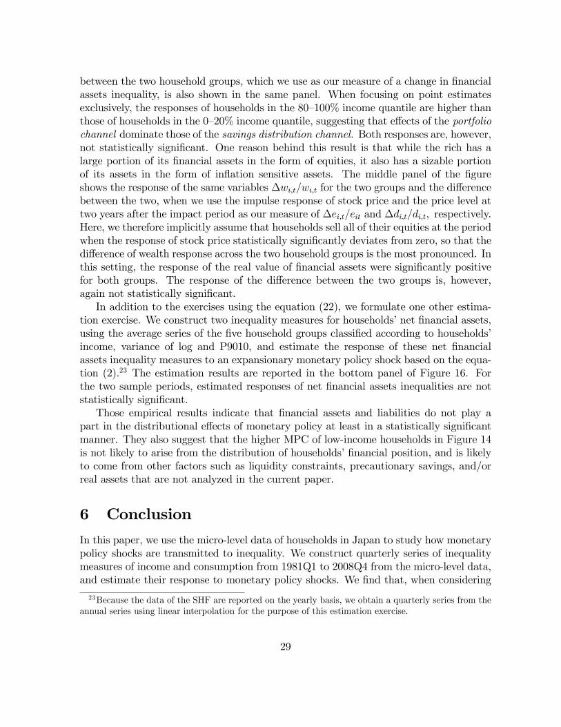
between the two household groups, which we use as our measure of a change in �nancialassets inequality, is also shown in the same panel. When focusing on point estimatesexclusively, the responses of households in the 80�100% income quantile are higher thanthose of households in the 0�20% income quantile, suggesting that e¤ects of the portfoliochannel dominate those of the savings distribution channel. Both responses are, however,not statistically signi�cant. One reason behind this result is that while the rich has alarge portion of its �nancial assets in the form of equities, it also has a sizable portionof its assets in the form of in�ation sensitive assets. The middle panel of the �gureshows the response of the same variables �wi;t=wi;t for the two groups and the di¤erencebetween the two, when we use the impulse response of stock price and the price level attwo years after the impact period as our measure of �ei;t=eit and �di;t=di;t; respectively.Here, we therefore implicitly assume that households sell all of their equities at the periodwhen the response of stock price statistically signi�cantly deviates from zero, so that thedi¤erence of wealth response across the two household groups is the most pronounced. Inthis setting, the response of the real value of �nancial assets were signi�cantly positivefor both groups. The response of the di¤erence between the two groups is, however,again not statistically signi�cant.In addition to the exercises using the equation (22), we formulate one other estima-

tion exercise. We construct two inequality measures for households�net �nancial assets,using the average series of the �ve household groups classi�ed according to households�income, variance of log and P9010, and estimate the response of these net �nancialassets inequality measures to an expansionary monetary policy shock based on the equa-tion (2).23 The estimation results are reported in the bottom panel of Figure 16. Forthe two sample periods, estimated responses of net �nancial assets inequalities are notstatistically signi�cant.Those empirical results indicate that �nancial assets and liabilities do not play a

part in the distributional e¤ects of monetary policy at least in a statistically signi�cantmanner. They also suggest that the higher MPC of low-income households in Figure 14is not likely to arise from the distribution of households��nancial position, and is likelyto come from other factors such as liquidity constraints, precautionary savings, and/orreal assets that are not analyzed in the current paper.

6 Conclusion

In this paper, we use the micro-level data of households in Japan to study how monetarypolicy shocks are transmitted to inequality. We construct quarterly series of inequalitymeasures of income and consumption from 1981Q1 to 2008Q4 from the micro-level data,and estimate their response to monetary policy shocks. We �nd that, when considering

23Because the data of the SHF are reported on the yearly basis, we obtain a quarterly series from theannual series using linear interpolation for the purpose of this estimation exercise.

29

inequality across households whose head is employed exclusively, an expansionary mon-etary policy shock increased income inequality through a rise in earnings inequality, inthe period before the 2000s. Such procyclical responses are, however, scarcely observedwhen the most current data is included in the sample period, or when earnings inequalityacross all households is considered. Regarding the transmission from income inequalityto consumption inequality, we �nd that the transmission is minor even during the periodbefore the 2000s, namely the period when procyclicality of income inequality followingmonetary policy shocks was pronounced. These observations suggest that the distribu-tional e¤ects of monetary policy shocks were once present, but they are not stable overtime, and possibly statistically insigni�cant, so far as the e¤ects on all households atpresent time are concerned.We show, using a simple dynamic general equilibrium model, that labor market �ex-

ibility is central to the dynamics of income inequality after monetary policy shocks inJapan. Given monetary policy shocks have heterogenous impacts on economic activityin di¤erent parts of the economy, the distributional e¤ects of monetary policy shocksdepend crucially on how labor markets react to the shocks. When labor markets aresegmented and mobility across �rms is limited, then heterogenous impacts on various�rms are easily translated into earnings inequality across workers. By contrast, when la-bor markets enjoy high �exibility, the heterogenous impacts on production do not causelarge distributional e¤ects across workers. The increasing �exibility of labor markets inJapan is consistent with our empirical observations regarding the response of earningsinequality to monetary policy shocks.In addition, we use the micro-level data of households��nancial assets and liabilities

to study the distributional e¤ects of monetary policy through changes in asset values.We �nd that �nancial assets and liabilities of Japanese households are distributed in away that both the portfolio channel and saving redistribution channel can work at leastqualitatively. However, the estimated e¤ects of expansionary monetary policy shocks onthe di¤erence across households in terms of the value of net assets is not signi�cantlydi¤erent from zero, throughout the sample period, indicating hat the two channels arenot quantitatively important in shaping the distributional e¤ects of monetary policy.Lastly, it is also important to distinguish the two sides of the same coin. A higher

�exibility of labor markets has two di¤erent implications for developments in inequal-ity. First, as the current paper highlights, an increase in the participation of temporaryworkers and an enhanced mobility of workers in labor markets helps isolate variationsin goods production across �rms, from being straightforwardly translated into variationsin earnings across workers. Consequently, it makes dynamics of income inequality al-most neutral to monetary policy shocks. Second, by contrast, as observed in existingstudies, the use of temporary workers is typically associated with structural and long-lived dispersions in wage pro�le across workers within a �rm, which has the potential towiden earnings inequality across households. Given the fact that inequality measures inJapan from the 1980s onwards exhibit a secular positive trend as shown in Figure 1, a

30

detailed analysis of structural developments in inequality is essential for gaining a betterunderstanding of the quantitative aspects of inequality. This is, however, left for futureresearch.

31

References

[1] Aikman, D., O. Bush, A. M. Taylor (2016) �Monetary Versus MacroprudentialPolicies: Causal Impacts of Interest Rates and Credit Controls in the Era of the UKRadcli¤e Report,�NBER Working Paper No. 22380.

[2] Auclert, A. (2016) �Monetary Policy and the Redistribution Channel,�WorkingPaper, Stanford University.

[3] Barsky, R., C. L. House, M. Kimball (2007) �Sticky Price Models and DurableGoods,�American Economic Review, 97(3), pp. 984�998.

[4] Bernanke, B. (2015) �Monetary Policy and Inequality,�Brookings Institution, June1st, 2015.

[5] Bernanke, B., J. Boivin, P. Eliasz (2005) �Measuring the E¤ects of Monetary Pol-icy: A Factor-Augmented Vector Autoregressive (FAVAR) Approach,�QuarterlyJournal of Economics, 120(1), pp. 387�422.

[6] Blundell, R., L. Pistaferri, I. Preston (2008) �Consumption Inequality and PartialInsurance,�American Economic Review, 98(5), pp. 1887�1921.

[7] Boivin, J., M. P. Giannoni, I. Mihov (2009) �Sticky Prices and Monetary Policy:Evidence from Disaggregated US Data,�American Economic Review, 99(1), pp.350�84.

[8] Braun, A. R., J. Esteban-Pretel, T. Okada, N. Sudou (2006) �A Comparison ofthe Japanese and U.S. Business Cycles,�Japan and the World Economy, 18(4), pp.441�463.

[9] Carroll, C. D., and M. Kimball (1996) �On the Concavity of the ConsumptionFunction.�Econometrica, 64 (4), pp. 981�92.

[10] Cohan, D. W. (2014) �How Quantitative Easing Contributed to the Nation�s In-equality Problem,�the New York Times, 22nd October, 2014.

[11] Coibion, O., Y. Gorodnichenko, L. Kueng, J. Silvia (2012) �Innocent Bystanders?Monetary Policy and Inequality in the U.S.,�NBER Working Paper No. 18170.

[12] Doepke, M., M. Schneider (2006) �In�ation and the Redistribution of NominalWealth,�Journal of Political Economy, 114(6), pp. 1069�1097.

[13] Doepke, M., M. Schneider, V. Selezneva (2015) �Distributional E¤ects of MonetaryPolicy,�Meeting Papers 1099, Society for Economic Dynamics.

32

[14] Domanski, D., M. Scatigna, A. Zabai (2016) �Wealth Inequality and MonetaryPolicy,�BIS Quarterly Review.

[15] Erceg, C., A. Levin (2006) �Optimal monetary policy with durable consumptiongoods,�Journal of Monetary Economics, 53(7), pp. 1341�1359.

[16] Furceri, D., P. Loungani, A. Zdzienicka (2016) �The E¤ects of Monetary PolicyShocks on Inequality,�IMF Working Papers 16/245.

[17] Gertler M., S. Gilchrist (1994) �Monetary Policy, Business Cycles, and the Behaviorof Small Manufacturing Firms,�The Quarterly Journal of Economics, 109(2), pp.309�340.

[18] Gornemann N., K. Kuester, M. Nakajima (2016) �Doves for the Rich, Hawks forthe Poor? Distributional Consequences of Monetary Policy,�International FinanceDiscussion Papers 1167, Board of Governors of the Federal Reserve System.

[19] Hayashi F., E. Prescott (2002) �The 1990s in Japan: A Lost Decade,�Review ofEconomic Dynamics, 5, pp. 206�235.

[20] Jappelli T., L. Pistaferri (2014) �Fiscal Policy and MPC Heterogeneity,�AmericanEconomic Journal: Macroeconomics, 6(4), pp. 107�136, October.

[21] Jordà, Ò (2005) �Estimation and Inference of Impulse Responses by Local Projec-tions,�American Economic Review, 95(1), pp. 161�182.

[22] Korinek, A., A. Simsek (2016) �Liquidity Trap and Excessive Leverage,�AmericanEconomic Review, 106(3), pp. 699�738.

[23] Krippner, L (2015) Zero Lower Bound Term Structure Modeling, Palgrave Macmil-lan.

[24] Krugman, P. (2014) �Notes on Easy Money and Inequality,�The Opinion Pages,The New York Times, 25th October, 2014.

[25] Lise, J., N. Sudo, M. Suzuki, K. Yamada, T. Yamada (2014) �Wage, Income andConsumption Inequality in Japan, 1981-2008: from Boom to Lost Decades,�Reviewof Economic Dynamics, 17(4), pp. 582�612.

[26] McKay A., E. Nakamura, J. Steinsson (2016) �The Power of Forward GuidanceRevisited,�American Economic Review, 106(10), pp. 3133�3158.

[27] Mumtaz, H., A. Theophilopoulou (2016) �The Impact of Monetary Policy on In-equality in the UK. An Empirical Analysis,�Working Papers 783, Queen MaryUniversity of London, School of Economics and Finance.

33

[28] Nakajima, M. (2015) �The Redistributive Consequences of Monetary Policy,�Busi-ness Review, Federal Reserve Bank of Philadelphia, issue Q2, pp. 9�16.

[29] Newey, W., K. West (1987) �A Simple, Positive Semi-de�nite, Heteroskedasticityand Autocorrelation Consistent Covariance Matrix,�Econometrica, 55(3) pp. 703�708.

[30] Oda, T. (2016) �Optimal In�ation Rate in a Life-Cycle Economy,�IMES DiscussionPaper Series 16-E-5, Institute for Monetary and Economic Studies, Bank of Japan.

[31] O�Farrell R., ×. Rawdanowicz, K. Inaba (2016) �Monetary Policy and Inequality,�OECD Economics Deparment Working Papers, 1281.

[32] Ohanian, L. E., A. C. Stockman, L. Kilian (1995) �The E¤ects of Real and MonetaryShocks in a Business Cycle Model with Some Sticky Prices,� Journal of Money,Credit, and Banking, 27, pp. 1209�1234.

[33] Peersman G., F. Smets (2005) �The Industry E¤ects of Monetary Policy in the EuroArea,�Economic Journal, 115(503), pp. 319�342.

[34] Piketty, T. (2014) Capital in the Twenty-First Century, Cambridge Massachusetts: The Belknap Press of Harvard University Press.

[35] Saiki, A., J. Frost (2014) �Does Unconventional Monetary Policy A¤ect Inequality?Evidence from Japan,�Applied Economics, 46, pp. 4445�4454.

[36] Ueno, Y. (2017) �Term Structure Models with Negative Interest Rates,� IMESDiscussion Paper Series 17-E-1, Institute for Monetary and Economic Studies, Bankof Japan.

[37] Wu, J. C., F. D. Xia (2016) �Measuring the Macroeconomic Impact of MonetaryPolicy at the Zero Lower Bound,�Journal of Money, Credit, and Banking, 48, pp.253�291.

34

A Appendix A

This appendix documents the data sources, including two micro-level data, the FIES andSHF, and the construction methodology of the time series of inequality measures usedin Section 4 and 5.

A.1 The Family Income and Expenditures Survey

A.1.1 About the FIES

The Family Income and Expenditure Survey (FIES) is a cross-sectional household surveyconducted monthly by the Japanese Ministry of Internal A¤airs and Communications.The FIES is a primary source of the private consumption series in the System of NationalAccounts (SNA). It is also used for the construction of the Consumption Price Index(CPI). Using this data, Lise et al. (2014) documents developments in inequality inJapan.The survey unit is a household and the universe for the survey includes all Japanese

households with the exception of (i) institutional households; (ii) students living alone;(iii) households in which the household business is a restaurant, or boarding house whichshares the same dwelling; (iv) households with boarders who share meals (even if this isnot the main source of income); (v) households with four or more live-in employees; (vi)households where the head is absent for more than three months in the year; and (vii)foreigners. Multiple-person households are surveyed for six consecutive months, whilesingle-person households are surveyed for three consecutive months, but only after 2002.One-sixth of the households are rotated out and replaced by new households every month.Approximately 8000 multiple-person households are surveyed every month, meaning thatapproximately 16,000 households are surveyed every year.The survey contains rich information on the earnings of household members, house-

hold consumption expenditures, and households�characteristics such as household mem-bers�ages, gender, occupation, industry of employment, marital status, and region ofresidence; however, detailed information on monthly income is collected only if the house-hold head is employed, but not if the household head is non-employed, self-employed,executive, free lancer, farmer, forester, or �sher. The household head is de�ned as the pri-mary earner in the household. The data is collected by a combination of survey questionsand a household diary in which households are requested to �ll in daily expenditures.There is neither bottom nor top coding of income and consumption records.

A.1.2 Variables of interest

We are interested in analyzing the inequality measures of �ve variables, earnings yL,pre-tax income y, disposable income yD, non-durable consumption cND, and total con-sumption expenditures cT . We refer to the last two variables simply as consumption and

35

expenditure. We de�ne each variable following Lise et al. (2014). Earnings yL is de�nedas the sum of earnings of all household members, namely household head, spouse, andother household members. As noted in the main text, however, when earnings are zero,we drop the household from our sample. Pre-tax income (y) is computed by adding assetincome and private transfers to the earnings (yL). We subtract reported tax paymentsfrom the pre-tax income and add public transfers to obtain disposable income (yD).The nondurable expenditure (cND) includes food (1), repair and maintenance (2.2), fuel,light and water charges (3), domestic utensils (4.4), domestic nondurable goods (4.5),domestic services (4.6), clothing and footwear (5), medical care (6), transportation andcommunication (7) (excluding purchase of vehicles (7.2.1) and bicycles (7.2.2)), educa-tion (8), culture and recreation (9) (excluding recreation durable goods (9.1)), and otherconsumption expenditures (10) (excluding remittance (10.4)).24 We add semidurable anddurable expenditures to cND to compute total consumption cT .

A.1.3 Construction methodology of quarterly series of inequality measures

Since the FIES is surveyed monthly, we construct a quarterly series of inequality measuresusing the data of households who are interviewed for three consecutive months within thequarter. We make two adjustments to the series. First, in order to control for di¤erencesin inequality measures arising from the size and composition of households, we equivalizeraw numbers using the OECD equivalent scale,25 and compute inequality measures acrosshouseholds based on these equivalized �gures. Second, we apply seasonal adjustmentsto the data. Our earnings series exhibits a strong seasonality due to bonuses that arepaid twice a year, one in summer (June or July), and one in winter (December). Whenconstructing quarterly series, therefore, we compute the total bonus payments for eachhousehold and distribute one-sixth of the bonus payments to regular monthly earnings,and apply the X12 ARIMA �lter to the series.

A.2 The Survey of Household Finances

A.2.1 About the SHF

The SHF is a cross-sectional household survey conducted by the Central Council forFinancial Services Information. Beginning in 1953, the survey, originally named the�Public Opinion Survey on Household Financial Assets and Liabilities�was renamed theSHF in 2007. The survey unit is a household and the universe for the survey includesall Japanese households that meet the following conditions; (i) households are multiple-person, and (ii) the household head is aged 20 or over. 8,000 multiple-person households

24Numbers in parentheses are the item codes in the FIES.25The OECD scale gives a unit weight to the �rst adult, 0.7 to all other adults, and 0.5 to children

aged 16 and younger.

36

are surveyed once a year.26 Sample households are selected each year.The survey contains rich information on the amount of �nancial assets and liabilities

by class, and selection of �nancial products such as stocks, bonds, deposits, insurance,and debt. The survey also details various characteristics of households such as income,expenditure, borrowing, education, and so forth.

A.2.2 Adjustments to variables of interest

Our interest is to assess the distributional e¤ects of expansionary monetary policy shocksvia changes in the value of households��nancial assets and liabilities. We construct thetime-series data of �nancial assets, stock holdings and �nancial liabilities by households�income quantiles. In order to maintain the consistency with our analysis using the FIESdata, we use only the data of households whose heads are aged from 25 to 59. Wealso drop households whose earnings are zero from our sample, for the same reason.Financial assets are de�ned as the total amount of �nancial products (excluding cash-in-hand, but including foreign currency-denominated �nancial products), as in the SHF.Stock holdings include employee stock ownership plans and foreign currency-denominatedstocks (in yen terms). We de�ne �nancial liabilities as the total outstanding balanceborrowed, which includes housing loans and educational loans.

A.3 Macroeconomic variables

A.3.1 Unobservable macroeconomic factors

In estimating the two equations (2) and (3), we useK unobserved macroeconomic factorsthat are extracted from a balanced panel that includes a quarterly series of 59 variablesfrom 1981Q1 to 2008Q4. The list of variables included in the panel is given in Table 2.All of the variables are transformed to stationary series by the methodology reported inthe table. From the balanced panel, we extract the time series of a set of unobservablefactors ~Ft as the �rst K principal components. We set the number of unobservable factorK to equal two in our baseline speci�cation. For a sensitivity analysis, which we reportin Appendix C, we estimate impulse response functions in a setting where K is set to 3instead of 2.

A.3.2 Total factor productivity

As in Hayashi and Prescott (2002), our measured TFP series, TFPt; is computed fromthe logarithm of output growth less the weighted average of the logarithm of laborinput and capital input growth. The time series of output and capital inputs are takenfrom the System of National Accounts, and that of labor input is obtained from the

26Note that not all households surveyed respond. In the 2015 survey, for example, 3,474 multiple-person households responded.

37

number of employees based on the Labour Force Survey, multiplied by hours workedper employee based on the Monthly Labour Survey. There are two di¤erences betweenour TFP series and that of Hayashi and Prescott (2002): (i) the output series that isused for constructing our TFP series is the GDP series, while the output series used forconstructing their TFP is GNP less government capital consumption; and (ii) households�residential and foreign assets are not included in our capital stock series, while these twocomponents are included by Hayashi and Prescott (2002).

38

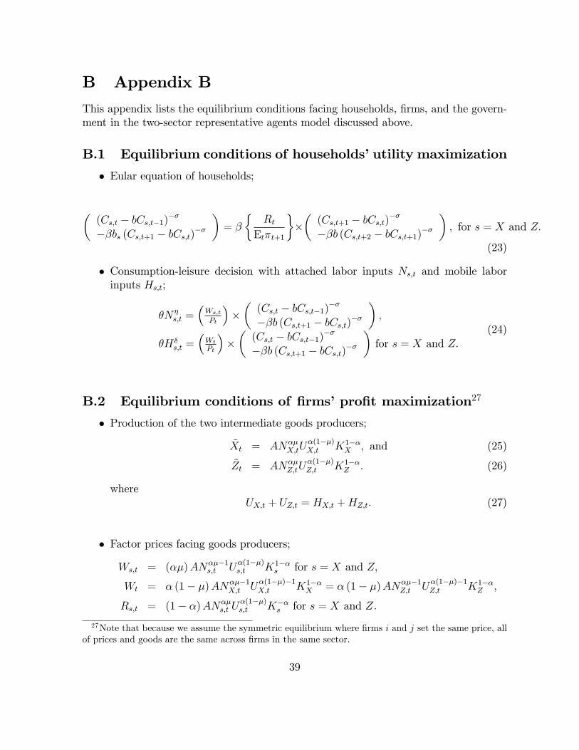
B Appendix B

This appendix lists the equilibrium conditions facing households, �rms, and the govern-ment in the two-sector representative agents model discussed above.

B.1 Equilibrium conditions of households�utility maximization

� Eular equation of households;

�(Cs;t � bCs;t�1)����bs (Cs;t+1 � bCs;t)��

�= �

�Rt

Et�t+1

���(Cs;t+1 � bCs;t)����b (Cs;t+2 � bCs;t+1)��

�; for s = X and Z:

(23)

� Consumption-leisure decision with attached labor inputs Ns;t and mobile laborinputs Hs;t;

�N�s;t =

�Ws;t

Pt

���(Cs;t � bCs;t�1)����b (Cs;t+1 � bCs;t)��

�;

�H�s;t =

�Wt

Pt

���(Cs;t � bCs;t�1)����b (Cs;t+1 � bCs;t)��

�for s = X and Z:

(24)

B.2 Equilibrium conditions of �rms�pro�t maximization27

� Production of the two intermediate goods producers;

~Xt = AN��X;tU

�(1��)X;t K1��

X ; and (25)

~Zt = AN��Z;tU

�(1��)Z;t K1��

Z : (26)

whereUX;t + UZ;t = HX;t +HZ;t: (27)

� Factor prices facing goods producers;

Ws;t = (��)AN���1s;t U

�(1��)s;t K1��

s for s = X and Z;

Wt = � (1� �)AN���1X;t U

�(1��)�1X;t K1��

X = � (1� �)AN���1Z;t U

�(1��)�1Z;t K1��

Z ;

Rs;t = (1� �)AN��s;t U

�(1��)s;t K��

s for s = X and Z.

27Note that because we assume the symmetric equilibrium where �rms i and j set the same price, allof prices and goods are the same across �rms in the same sector.

39

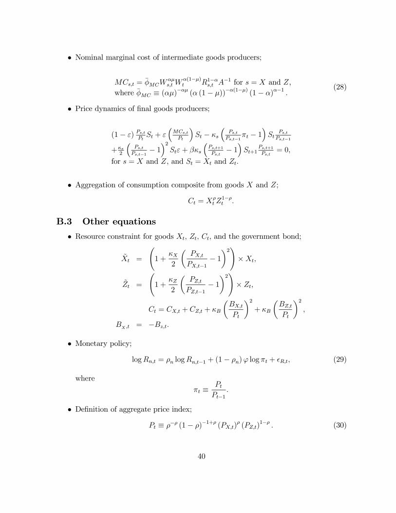
� Nominal marginal cost of intermediate goods producers;

MCs;t = ��MCW��s;t W

�(1��)t R1��s;t A

�1 for s = X and Z,where ��MC � (��)

��� (� (1� �))��(1��) (1� �)��1 :(28)

� Price dynamics of �nal goods producers;

(1� ") Ps;tPtSt + "

�MCs;tPt

�St � �s

�Ps;tPs;t�1

�t � 1�St

Ps;tPs;t�1

+�s2

�Ps;tPs;t�1

� 1�2St"+ ��s

�Ps;t+1Ps;t

� 1�St+1

Ps;t+1Ps;t

= 0;

for s = X and Z, and St = Xt and Zt:

� Aggregation of consumption composite from goods X and Z;

Ct = X�t Z

1��t :

B.3 Other equations

� Resource constraint for goods Xt; Zt; Ct; and the government bond;

~Xt =

1 +

�X2

�PX;tPX;t�1

� 1�2!

�Xt;

~Zt =

1 +

�Z2

�PZ;tPZ;t�1

� 1�2!

� Zt;

Ct = CX;t + CZ;t + �B

�BX;tPt

�2+ �B

�BZ;tPt

�2;

BX ;t = �Bz;t:

� Monetary policy;

logRn;t = �n logRn;t�1 + (1� �n)' log �t + �R;t; (29)

where

�t �PtPt�1

:

� De�nition of aggregate price index;

Pt � ��� (1� �)�1+� (PX;t)� (PZ;t)1�� : (30)

40

C Appendix C

This appendix serves for the sensitivity analysis of our empirical results. We conduct fourdi¤erent estimation exercises to as to formulate exercises shown in Figures 4 and 5 in themain text under the following settings: (i) estimation using the shadow rate constructedby Krippner (2015), instead of the shadow rate of Ueno (2017), as the policy rate Rt, (ii)estimation using the two-year government bond yield, instead of the shadow rate of Ueno(2017), as the policy rate Rt, (iii) estimation that sets the number of unobservable factorsK = 3; instead of K = 2; and (iv) estimation that sets the ordering of macroeconomicvariables Mt in the estimation equation so that the short-term interest rate Rt comes�rst, instead of the setting where the short-term interest rate Rt is the least exogenous tothe system. Note that for all of the four exercises, estimation procedures are unchangedfrom those of the baseline estimation except for the procedure speci�ed above.The �rst two exercises intend to examine the robustness of our results to the use of

alternative measures of the monetary policy instrument. Note also that in the secondsetting, we use the two-year government bond yield for estimates of both sample periods,1981Q1 to 1998Q4, and 1981Q1 to 2008Q4. The third exercise intends to examine therobustness to a change in the number of factors. The fourth exercises intends to checkthe robustness when alternative relationship between a monetary policy shock and othermacroeconomic factors is considered:Figures C1 to C4 show the estimation results under the four alternative settings, (i);

(ii); (iii); and (iv):While there are some di¤erences across settings, to a greater or lesserdegree, the key observations are robust to the estimation methodologies.

41

Table 1: Model ParametersDescription

� :999 Discount factorb :5 Degree of habit formation

� and � 1 Utility weight attached to attached and mobile labor inputs� and � 1 Frisch elasticity of labor supply of attached and mobile labor inputs

KXand KZ

:5 Share of a household�s ownership of capital stock �X and �Z :5 Share of a household�s ownership of �rms

�B 10 Adjustment cost associated with bond holdingsA 1 Technology level� :65 Labor share in goods production� :6 Share of attached labor inputsKX 1 Aggregate capital stock in sector XKZ 1 Aggregate capital stock in sector Z� :51 Share of goods X in the aggregate composite Ct" 11 Price elasticity of di¤erentiated goods�X 500 Adjustment cost associated with price setting in sector X�Z 50 Adjustment cost associated with price setting in sector Z�n :9 Persistence of the policy rate' 1:5 Policy weight attached to in�ation rate

42

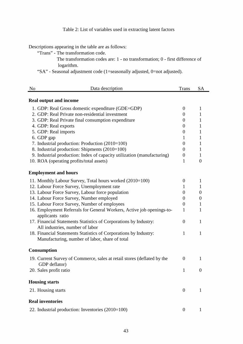
43

No Trans SA

Real output and income1. GDP: Real Gross domestic expenditure (GDE=GDP) 0 12. GDP: Real Private non-residential investment 0 13. GDP: Real Private final consumption expenditure 0 14. GDP: Real exports 0 15. GDP: Real imports 0 16. GDP gap 1 17. Industrial production: Production (2010=100) 0 18. Industrial production: Shipments (2010=100) 0 19. Industrial production: Index of capacity utilization (manufacturing) 0 1

10. ROA (operating profits/total assets) 1 0

Employment and hours11. Monthly Labour Survey, Total hours worked (2010=100) 0 112. Labour Force Survey, Unemployment rate 1 113. Labour Force Survey, Labour force population 0 014. Labour Force Survey, Number employed 0 015. Labour Force Survey, Number of employees 0 116. Employment Referrals for General Workers, Active job openings-to- 1 1

applicants ratio17. Financial Statements Statistics of Corporations by Industry: 0 1

All industries, number of labor18. Financial Statements Statistics of Corporations by Industry: 1 1

Manufacturing, number of labor, share of total

Consumption

19. Current Survey of Commerce, sales at retail stores (deflated by the 0 1 GDP deflator)

20. Sales profit ratio 1 0

Housing starts

21. Housing starts 0 1

Real inventories

22. Industrial production: Inventories (2010=100) 0 1

Table 2: List of variables used in extracting latent factors

Descriptions appearing in the table are as follows: “Trans” - The transformation code. The transformation codes are: 1 - no transformation; 0 - first difference of logarithm. “SA” - Seasonal adjustment code (1=seasonally adjusted, 0=not adjusted).

Data description

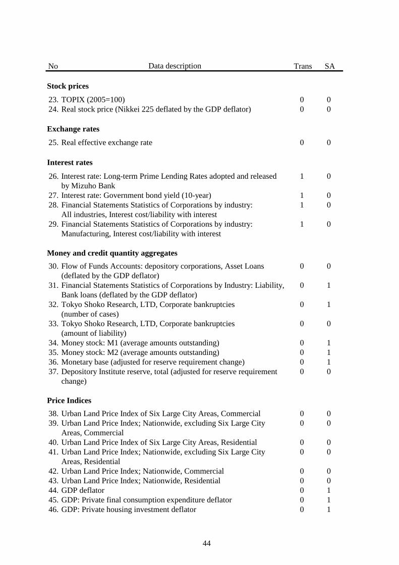
44

No Trans SA

Stock prices

23. TOPIX (2005=100) 0 024. Real stock price (Nikkei 225 deflated by the GDP deflator) 0 0

Exchange rates

25. Real effective exchange rate 0 0

Interest rates

26. Interest rate: Long-term Prime Lending Rates adopted and released 1 0by Mizuho Bank

27. Interest rate: Government bond yield (10-year) 1 028. Financial Statements Statistics of Corporations by industry: 1 0

All industries, Interest cost/liability with interest29. Financial Statements Statistics of Corporations by industry: 1 0

Manufacturing, Interest cost/liability with interest

Money and credit quantity aggregates30. Flow of Funds Accounts: depository corporations, Asset Loans 0 0

(deflated by the GDP deflator)31. Financial Statements Statistics of Corporations by Industry: Liability, 0 1

Bank loans (deflated by the GDP deflator)32. Tokyo Shoko Research, LTD, Corporate bankruptcies 0 1

(number of cases)33. Tokyo Shoko Research, LTD, Corporate bankruptcies 0 0

(amount of liability)34. Money stock: M1 (average amounts outstanding) 0 135. Money stock: M2 (average amounts outstanding) 0 136. Monetary base (adjusted for reserve requirement change) 0 137. Depository Institute reserve, total (adjusted for reserve requirement 0 0

change)

Price Indices38. Urban Land Price Index of Six Large City Areas, Commercial 0 039. Urban Land Price Index; Nationwide, excluding Six Large City 0 0

Areas, Commercial40. Urban Land Price Index of Six Large City Areas, Residential 0 041. Urban Land Price Index; Nationwide, excluding Six Large City 0 0

Areas, Residential42. Urban Land Price Index; Nationwide, Commercial 0 043. Urban Land Price Index; Nationwide, Residential 0 044. GDP deflator 0 145. GDP: Private final consumption expenditure deflator 0 146. GDP: Private housing investment deflator 0 1

Data description

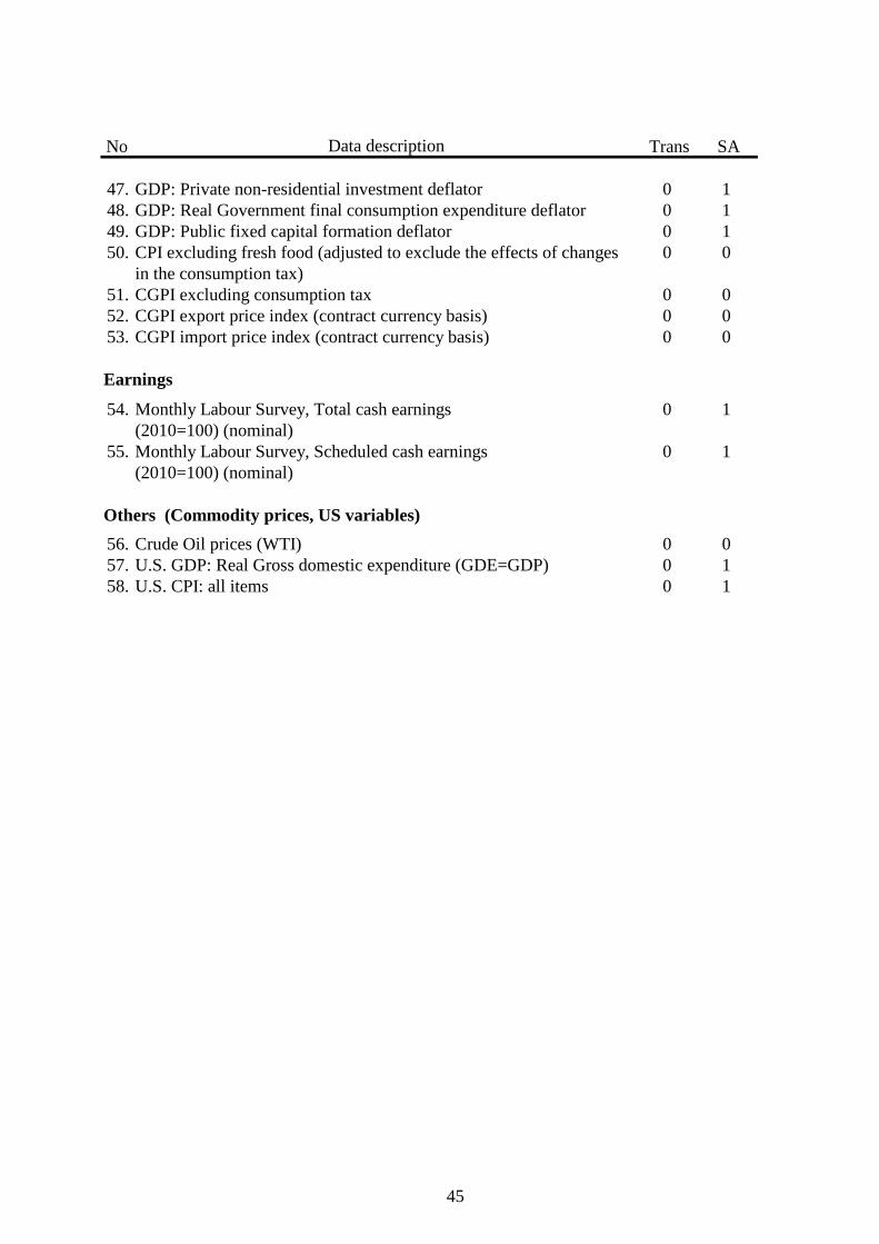
45

No Trans SA

47. GDP: Private non-residential investment deflator 0 148. GDP: Real Government final consumption expenditure deflator 0 149. GDP: Public fixed capital formation deflator 0 150. CPI excluding fresh food (adjusted to exclude the effects of changes 0 0

in the consumption tax)51. CGPI excluding consumption tax 0 052. CGPI export price index (contract currency basis) 0 053. CGPI import price index (contract currency basis) 0 0

Earnings

54. Monthly Labour Survey, Total cash earnings 0 1(2010=100) (nominal)

55. Monthly Labour Survey, Scheduled cash earnings 0 1(2010=100) (nominal)

Others (Commodity prices, US variables)56. Crude Oil prices (WTI) 0 057. U.S. GDP: Real Gross domestic expenditure (GDE=GDP) 0 158. U.S. CPI: all items 0 1

Data description

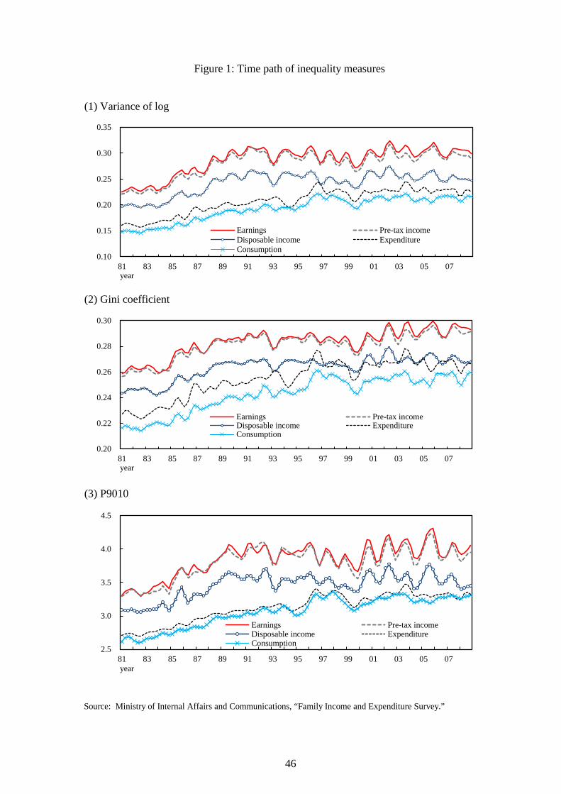
46

Figure 1: Time path of inequality measures

(1) Variance of log

(2) Gini coefficient

(3) P9010

Source: Ministry of Internal Affairs and Communications, “Family Income and Expenditure Survey.”

0.10

0.15

0.20

0.25

0.30

0.35

81 83 85 87 89 91 93 95 97 99 01 03 05 07

Earnings Pre-tax incomeDisposable income ExpenditureConsumption

year

0.20

0.22

0.24

0.26

0.28

0.30

81 83 85 87 89 91 93 95 97 99 01 03 05 07

Earnings Pre-tax incomeDisposable income ExpenditureConsumption

year

2.5

3.0

3.5

4.0

4.5

81 83 85 87 89 91 93 95 97 99 01 03 05 07

Earnings Pre-tax incomeDisposable income ExpenditureConsumption

year

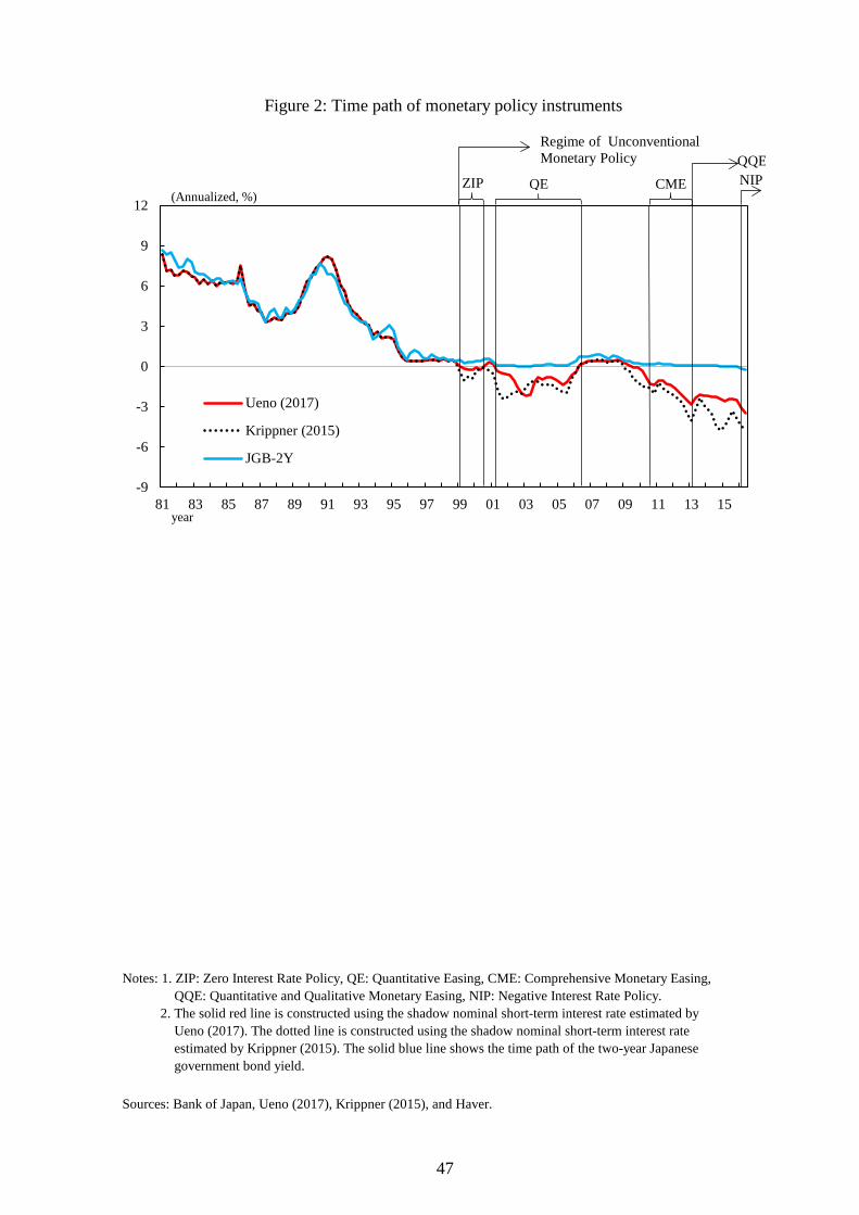
47

Figure 2: Time path of monetary policy instruments

Sources: Bank of Japan, Ueno (2017), Krippner (2015), and Haver.

Notes: 1. ZIP: Zero Interest Rate Policy, QE: Quantitative Easing, CME: Comprehensive Monetary Easing, QQE: Quantitative and Qualitative Monetary Easing, NIP: Negative Interest Rate Policy. 2. The solid red line is constructed using the shadow nominal short-term interest rate estimated by Ueno (2017). The dotted line is constructed using the shadow nominal short-term interest rate estimated by Krippner (2015). The solid blue line shows the time path of the two-year Japanese government bond yield.

-9

-6

-3

0

3

6

9

12

81 83 85 87 89 91 93 95 97 99 01 03 05 07 09 11 13 15

Ueno (2017)

Krippner (2015)

JGB-2Y

(Annualized, %)

year

ZIP QE CME QQE

Regime of Unconventional Monetary Policy

NIP

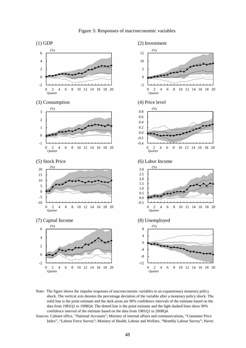
48

(1) GDP (2) Investment

(3) Consumption (4) Price level

(5) Stock Price (6) Labor Income

(7) Capital Income (8) Unemployed

Note: The figure shows the impulse responses of macroeconomic variables to an expansionary monetary policy shock. The vertical axis denotes the percentage deviation of the variable after a monetary policy shock. The solid line is the point estimate and the dark areas are 90% confidence intervals of the estimate based on the data from 1981Q1 to 1998Q4. The dotted line is the point estimate and the light dashed lines show 90% confidence interval of the estimate based on the data from 1981Q1 to 2008Q4.Sources: Cabinet office, “National Accounts”; Ministry of internal affairs and communications, “Consumer Price Index”, “Labour Force Survey”; Ministry of Health, Labour and Welfare, “Monthly Labour Survey”; Haver.

Figure 3: Responses of macroeconomic variables

-2

0

2

4

6

0 2 4 6 8 10 12 14 16 18 20

(%)

Quarter

-5

0

5

10

15

0 2 4 6 8 10 12 14 16 18 20

(%)

Quarter

-10-505

101520

0 2 4 6 8 10 12 14 16 18 20

(%)

Quarter

-0.50.00.51.01.52.02.53.0

0 2 4 6 8 10 12 14 16 18 20

(%)

Quarter

-1

0

1

2

3

0 2 4 6 8 10 12 14 16 18 20

(%)

Quarter

-0.4-0.20.00.20.40.60.8

0 2 4 6 8 10 12 14 16 18 20

(%)

Quarter

-2

0

2

4

6

0 2 4 6 8 10 12 14 16 18 20

(%)

Quarter

-12

-8

-4

0

4

8

0 2 4 6 8 10 12 14 16 18 20

(%)

Quarter

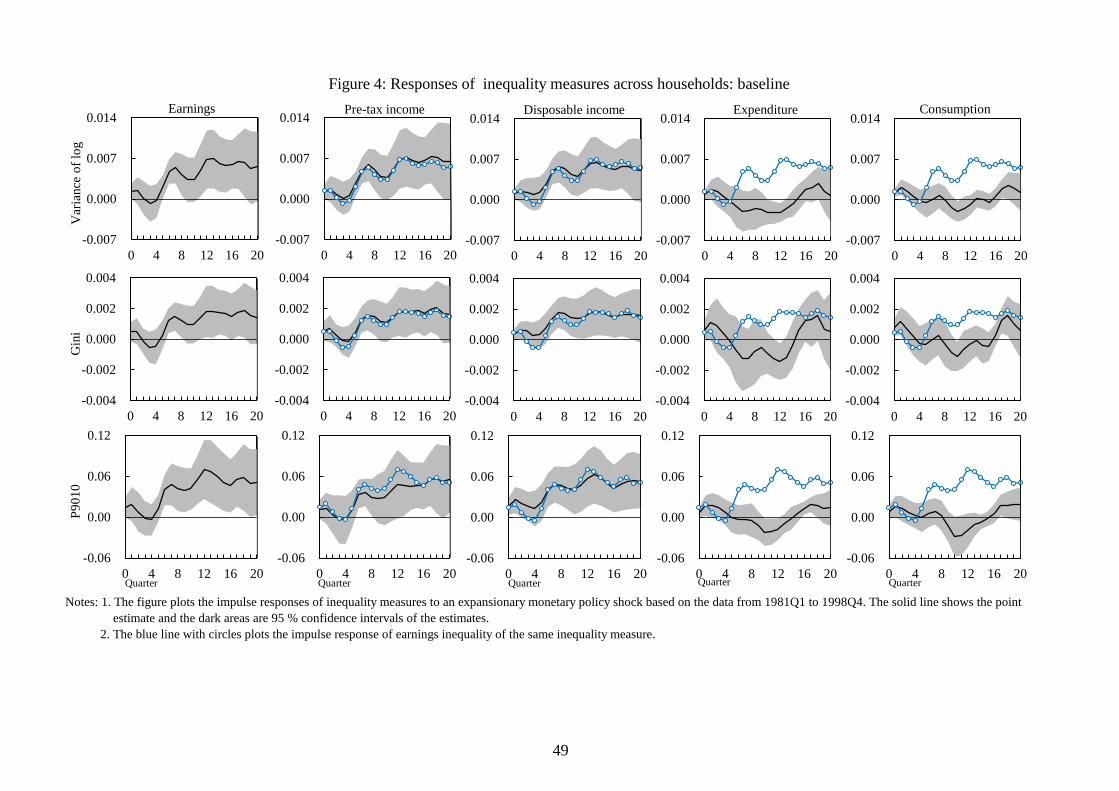
49

Figure 4: Responses of inequality measures across households: baseline

Notes: 1. The figure plots the impulse responses of inequality measures to an expansionary monetary policy shock based on the data from 1981Q1 to 1998Q4. The solid line shows the point estimate and the dark areas are 95 % confidence intervals of the estimates. 2. The blue line with circles plots the impulse response of earnings inequality of the same inequality measure.

-0.007

0.000

0.007

0.014

0 4 8 12 16 20

Earnings

Var

ianc

e of

log

-0.004

-0.002

0.000

0.002

0.004

0 4 8 12 16 20

Gin

i

-0.06

0.00

0.06

0.12

0 4 8 12 16 20Quarter

P901

0

-0.007

0.000

0.007

0.014

0 4 8 12 16 20

Pre-tax income

-0.004

-0.002

0.000

0.002

0.004

0 4 8 12 16 20

-0.06

0.00

0.06

0.12

0 4 8 12 16 20Quarter

-0.007

0.000

0.007

0.014

0 4 8 12 16 20

Disposable income

-0.004

-0.002

0.000

0.002

0.004

0 4 8 12 16 20

-0.06

0.00

0.06

0.12

0 4 8 12 16 20Quarter

-0.007

0.000

0.007

0.014

0 4 8 12 16 20

Expenditure

-0.004

-0.002

0.000

0.002

0.004

0 4 8 12 16 20

-0.06

0.00

0.06

0.12

0 4 8 12 16 20Quarter

-0.007

0.000

0.007

0.014

0 4 8 12 16 20

Consumption

-0.004

-0.002

0.000

0.002

0.004

0 4 8 12 16 20

-0.06

0.00

0.06

0.12

0 4 8 12 16 20Quarter

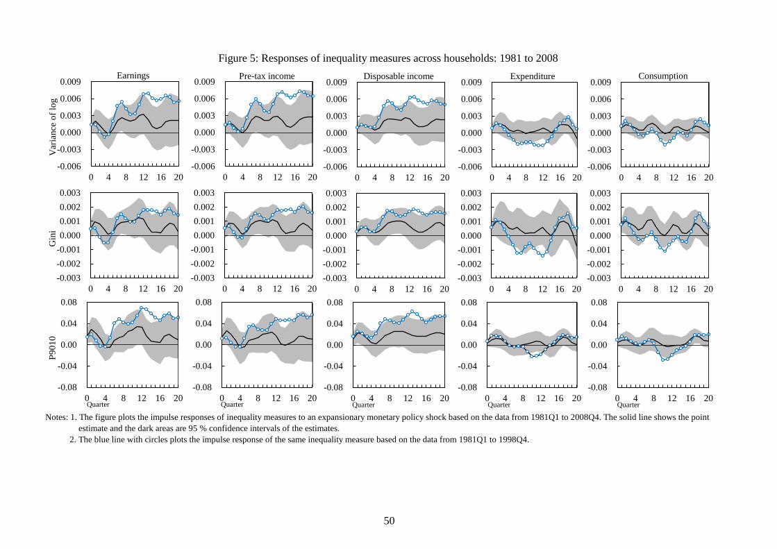
50

Figure 5: Responses of inequality measures across households: 1981 to 2008

Notes: 1. The figure plots the impulse responses of inequality measures to an expansionary monetary policy shock based on the data from 1981Q1 to 2008Q4. The solid line shows the point estimate and the dark areas are 95 % confidence intervals of the estimates. 2. The blue line with circles plots the impulse response of the same inequality measure based on the data from 1981Q1 to 1998Q4.

-0.006

-0.003

0.000

0.003

0.006

0.009

0 4 8 12 16 20

Earnings

Var

ianc

e of

log

-0.003-0.002-0.0010.0000.0010.0020.003

0 4 8 12 16 20

Gin

i

-0.08

-0.04

0.00

0.04

0.08

0 4 8 12 16 20Quarter

P901

0

-0.006

-0.003

0.000

0.003

0.006

0.009

0 4 8 12 16 20

Pre-tax income

-0.003-0.002-0.0010.0000.0010.0020.003

0 4 8 12 16 20

-0.08

-0.04

0.00

0.04

0.08

0 4 8 12 16 20Quarter

-0.006

-0.003

0.000

0.003

0.006

0.009

0 4 8 12 16 20

Disposable income

-0.003-0.002-0.0010.0000.0010.0020.003

0 4 8 12 16 20

-0.08

-0.04

0.00

0.04

0.08

0 4 8 12 16 20Quarter

-0.006

-0.003

0.000

0.003

0.006

0.009

0 4 8 12 16 20

Expenditure

-0.003-0.002-0.0010.0000.0010.0020.003

0 4 8 12 16 20

-0.08

-0.04

0.00

0.04

0.08

0 4 8 12 16 20Quarter

-0.006

-0.003

0.000

0.003

0.006

0.009

0 4 8 12 16 20

Consumption

-0.003-0.002-0.0010.0000.0010.0020.003

0 4 8 12 16 20

-0.08

-0.04

0.00

0.04

0.08

0 4 8 12 16 20Quarter

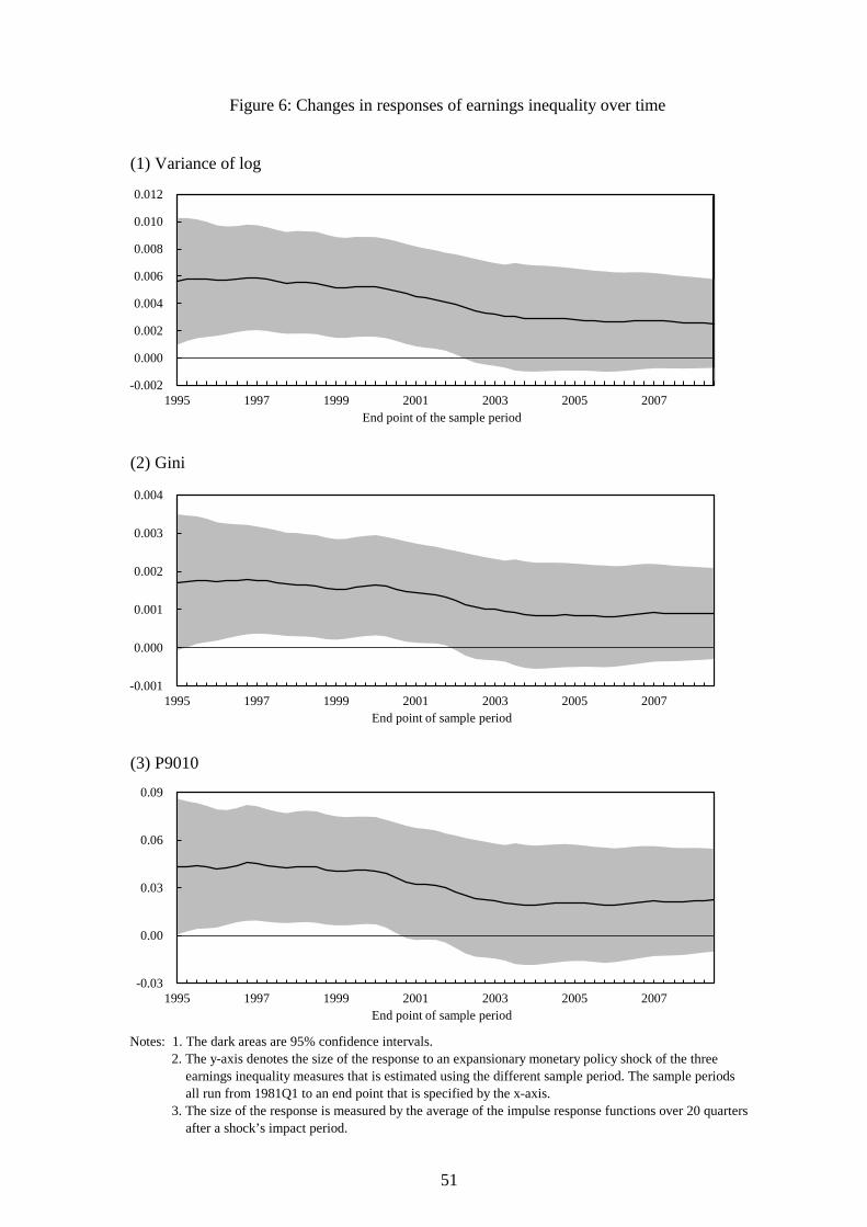
51

Figure 6: Changes in responses of earnings inequality over time

(1) Variance of log

(2) Gini

(3) P9010

Notes: 1. The dark areas are 95% confidence intervals. 2. The y-axis denotes the size of the response to an expansionary monetary policy shock of the three earnings inequality measures that is estimated using the different sample period. The sample periods all run from 1981Q1 to an end point that is specified by the x-axis. 3. The size of the response is measured by the average of the impulse response functions over 20 quarters after a shock’s impact period.

-0.001

0.000

0.001

0.002

0.003

0.004

1995 1997 1999 2001 2003 2005 2007End point of sample period

-0.002

0.000

0.002

0.004

0.006

0.008

0.010

0.012

1995 1997 1999 2001 2003 2005 2007End point of the sample period

-0.03

0.00

0.03

0.06

0.09

1995 1997 1999 2001 2003 2005 2007End point of sample period

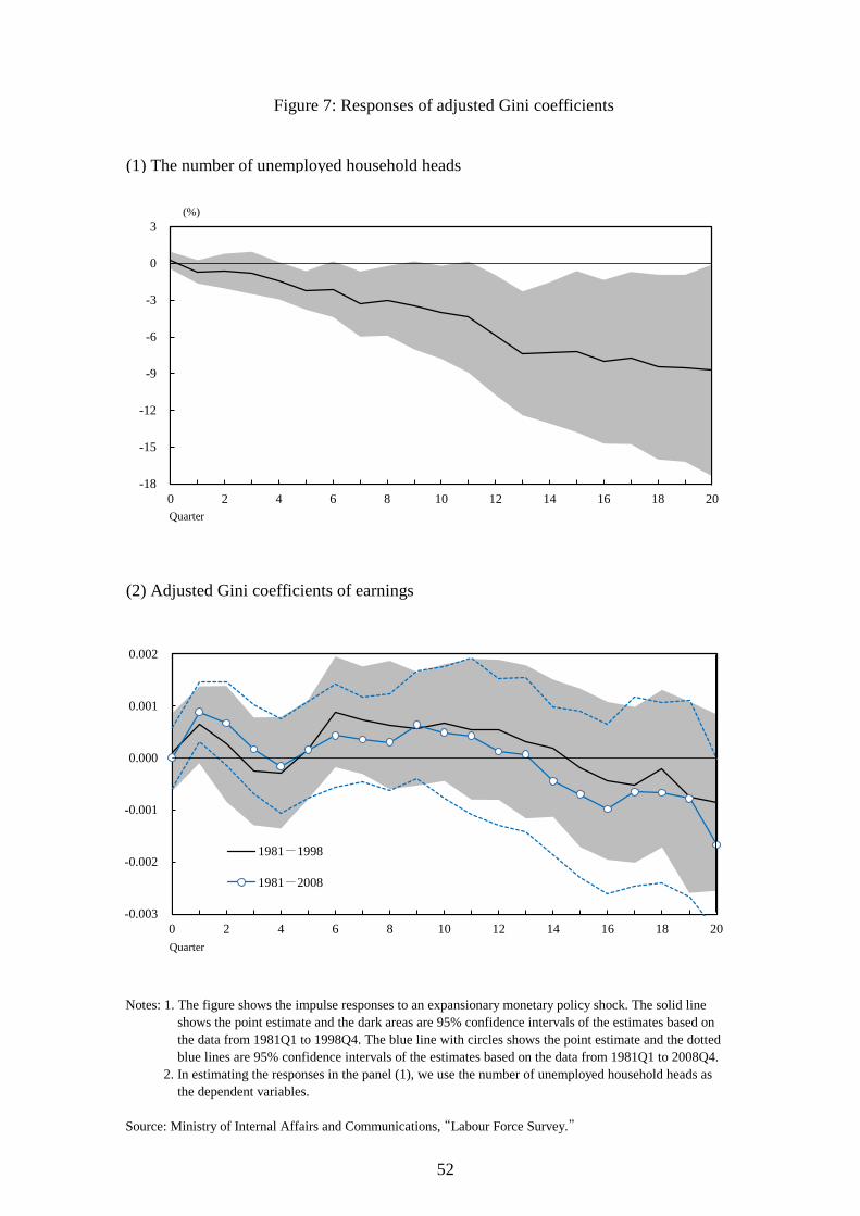
52

Figure 7: Responses of adjusted Gini coefficients

(2) Adjusted Gini coefficients of earnings

Notes: 1. The figure shows the impulse responses to an expansionary monetary policy shock. The solid line shows the point estimate and the dark areas are 95% confidence intervals of the estimates based on the data from 1981Q1 to 1998Q4. The blue line with circles shows the point estimate and the dotted blue lines are 95% confidence intervals of the estimates based on the data from 1981Q1 to 2008Q4. 2. In estimating the responses in the panel (1), we use the number of unemployed household heads as the dependent variables.

Source: Ministry of Internal Affairs and Communications, “Labour Force Survey.”

(1) The number of unemployed household heads

-0.003

-0.002

-0.001

0.000

0.001

0.002

0 2 4 6 8 10 12 14 16 18 20

1981－1998

1981－2008

Quarter

-18

-15

-12

-9

-6

-3

0

3

0 2 4 6 8 10 12 14 16 18 20Quarter

(%)

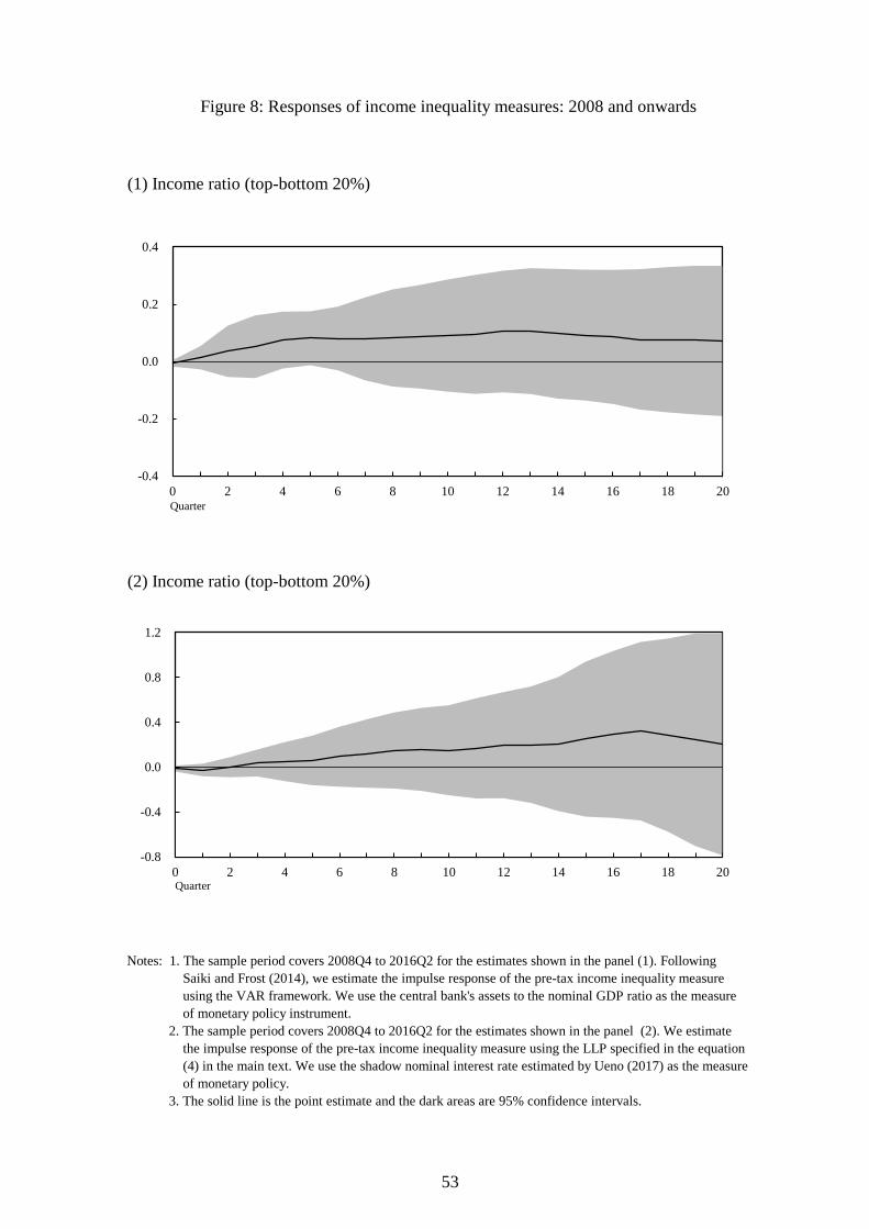
53

Figure 8: Responses of income inequality measures: 2008 and onwards

(1) Income ratio (top-bottom 20%)

(2) Income ratio (top-bottom 20%)

Notes: 1. The sample period covers 2008Q4 to 2016Q2 for the estimates shown in the panel (1). Following Saiki and Frost (2014), we estimate the impulse response of the pre-tax income inequality measure using the VAR framework. We use the central bank's assets to the nominal GDP ratio as the measure of monetary policy instrument. 2. The sample period covers 2008Q4 to 2016Q2 for the estimates shown in the panel (2). We estimate the impulse response of the pre-tax income inequality measure using the LLP specified in the equation (4) in the main text. We use the shadow nominal interest rate estimated by Ueno (2017) as the measure of monetary policy. 3. The solid line is the point estimate and the dark areas are 95% confidence intervals.

-0.4

-0.2

0.0

0.2

0.4

0 2 4 6 8 10 12 14 16 18 20Quarter

-0.8

-0.4

0.0

0.4

0.8

1.2

0 2 4 6 8 10 12 14 16 18 20Quarter

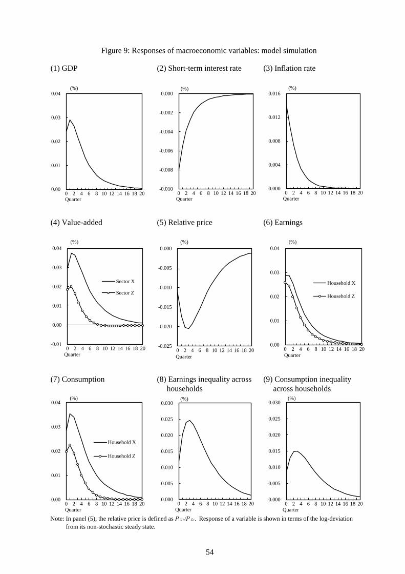
54

(1) GDP (2) Short-term interest rate (3) Inflation rate

(4) Value-added (5) Relative price (6) Earnings

(7) Consumption (8) Earnings inequality across (9) Consumption inequality households across households

Figure 9: Responses of macroeconomic variables: model simulation

Note: In panel (5), the relative price is defined as P X,t /P Z,t . Response of a variable is shown in terms of the log-deviation from its non-stochastic steady state.

0.00

0.01

0.02

0.03

0.04

0 2 4 6 8 10 12 14 16 18 20

Household X

Household Z

Quarter

(%)

0.00

0.01

0.02

0.03

0.04

0 2 4 6 8 10 12 14 16 18 20Quarter

(%)

-0.010

-0.008

-0.006

-0.004

-0.002

0.000

0 2 4 6 8 10 12 14 16 18 20Quarter

(%)

0.000

0.004

0.008

0.012

0.016

0 2 4 6 8 10 12 14 16 18 20Quarter

(%)

-0.01

0.00

0.01

0.02

0.03

0.04

0 2 4 6 8 10 12 14 16 18 20

Sector X

Sector Z

Quarter

(%)

-0.025

-0.020

-0.015

-0.010

-0.005

0.000

0 2 4 6 8 10 12 14 16 18 20Quarter

(%)

0.00

0.01

0.02

0.03

0.04

0 2 4 6 8 10 12 14 16 18 20

Household X

Household Z

Quarter

(%)

0.000

0.005

0.010

0.015

0.020

0.025

0.030

0 2 4 6 8 10 12 14 16 18 20Quarter

(%)

0.000

0.005

0.010

0.015

0.020

0.025

0.030

0 2 4 6 8 10 12 14 16 18 20Quarter

(%)

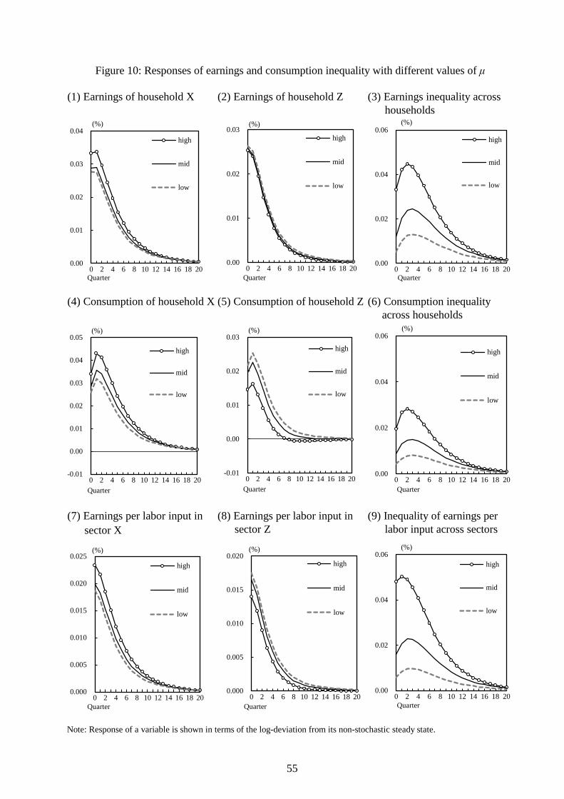
55

(1) Earnings of household X (2) Earnings of household Z (3) Earnings inequality across households

(4) Consumption of household X (5) Consumption of household Z (6) Consumption inequality across households

(7) Earnings per labor input in (8) Earnings per labor input in (9) Inequality of earnings per sector X sector Z labor input across sectors

Figure 10: Responses of earnings and consumption inequality with different values of μ

Note: Response of a variable is shown in terms of the log-deviation from its non-stochastic steady state.

0.00

0.02

0.04

0.06

0 2 4 6 8 10 12 14 16 18 20

high

mid

low

Quarter

(%)

0.00

0.02

0.04

0.06

0 2 4 6 8 10 12 14 16 18 20

high

mid

low

Quarter

(%)

0.00

0.01

0.02

0.03

0.04

0 2 4 6 8 10 12 14 16 18 20

high

mid

low

Quarter

(%)

0.00

0.01

0.02

0.03

0 2 4 6 8 10 12 14 16 18 20

high

mid

low

Quarter

(%)

-0.01

0.00

0.01

0.02

0.03

0.04

0.05

0 2 4 6 8 10 12 14 16 18 20

high

mid

low

Quarter

(%)

-0.01

0.00

0.01

0.02

0.03

0 2 4 6 8 10 12 14 16 18 20

high

mid

low

Quarter

(%)

0.00

0.02

0.04

0.06

0 2 4 6 8 10 12 14 16 18 20

high

mid

low

Quarter

(%)

0.000

0.005

0.010

0.015

0.020

0.025

0 2 4 6 8 10 12 14 16 18 20

high

mid

low

Quarter

(%)

0.000

0.005

0.010

0.015

0.020

0 2 4 6 8 10 12 14 16 18 20

high

mid

low

Quarter

(%)

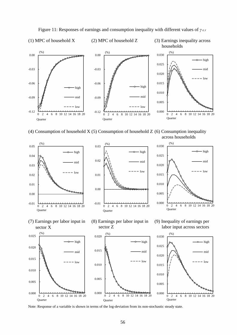
56

(1) MPC of household X (2) MPC of household Z (3) Earnings inequality across households

(4) Consumption of household X (5) Consumption of household Z (6) Consumption inequality across households

(7) Earnings per labor input in (8) Earnings per labor input in (9) Inequality of earnings per sector X sector Z labor input across sectors

Figure 11: Responses of earnings and consumption inequality with different values of γ K,X

Note: Response of a variable is shown in terms of the log-deviation from its non-stochastic steady state.

0.000

0.005

0.010

0.015

0.020

0.025

0.030

0 2 4 6 8 10 12 14 16 18 20

high

mid

low

Quarter

(%)

0.000

0.005

0.010

0.015

0.020

0.025

0.030

0 2 4 6 8 10 12 14 16 18 20

high

mid

low

Quarter

(%)

-0.01

0.00

0.01

0.02

0.03

0.04

0.05

0 2 4 6 8 10 12 14 16 18 20

high

mid

low

Quarter

(%)

-0.01

0.00

0.01

0.02

0.03

0 2 4 6 8 10 12 14 16 18 20

high

mid

low

Quarter

(%)

-0.12

-0.09

-0.06

-0.03

0.00

0 2 4 6 8 10 12 14 16 18 20

high

mid

low

Quarter

(%)

-0.12

-0.09

-0.06

-0.03

0.00

0 2 4 6 8 10 12 14 16 18 20

high

mid

low

Quarter

(%)

0.000

0.005

0.010

0.015

0.020

0.025

0.030

0 2 4 6 8 10 12 14 16 18 20

high

mid

low

Quarter

(%)

0.000

0.005

0.010

0.015

0.020

0.025

0 2 4 6 8 10 12 14 16 18 20

high

mid

low

Quarter

(%)

0.000

0.005

0.010

0.015

0.020

0 2 4 6 8 10 12 14 16 18 20

high

mid

low

Quarter

(%)

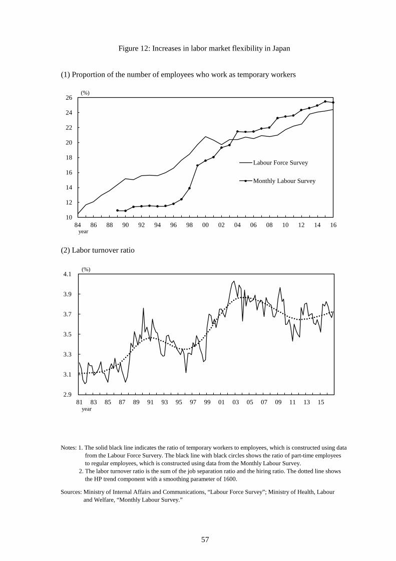
57

Figure 12: Increases in labor market flexibility in Japan

(1) Proportion of the number of employees who work as temporary workers

(2) Labor turnover ratio

Sources: Ministry of Internal Affairs and Communications, “Labour Force Survey”; Ministry of Health, Labour and Welfare, “Monthly Labour Survey.”

Notes: 1. The solid black line indicates the ratio of temporary workers to employees, which is constructed using data from the Labour Force Survery. The black line with black circles shows the ratio of part-time employees to regular employees, which is constructed using data from the Monthly Labour Survey. 2. The labor turnover ratio is the sum of the job separation ratio and the hiring ratio. The dotted line shows the HP trend component with a smoothing parameter of 1600.

10

12

14

16

18

20

22

24

26

84 86 88 90 92 94 96 98 00 02 04 06 08 10 12 14 16

Labour Force Survey

Monthly Labour Survey

year

(%)

2.9

3.1

3.3

3.5

3.7

3.9

4.1

81 83 85 87 89 91 93 95 97 99 01 03 05 07 09 11 13 15year

(%)

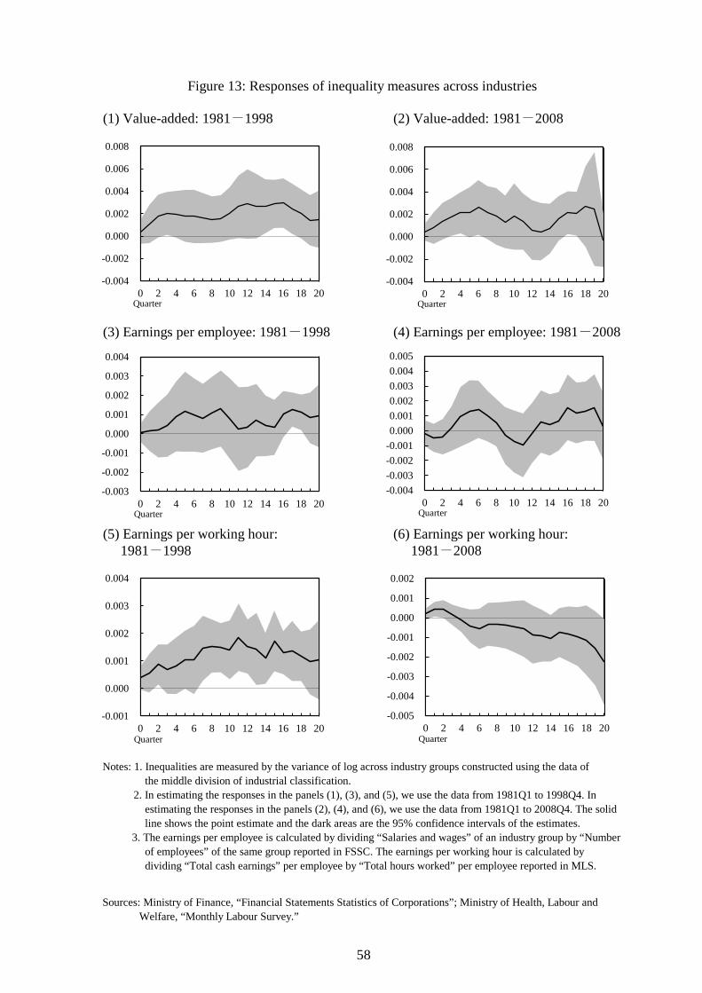
58

Figure 13: Responses of inequality measures across industries

(1) Value-added: 1981－1998 (2) Value-added: 1981－2008

(3) Earnings per employee: 1981－1998 (4) Earnings per employee: 1981－2008

(5) Earnings per working hour: (6) Earnings per working hour: 1981－1998 1981－2008

Notes: 1. Inequalities are measured by the variance of log across industry groups constructed using the data of the middle division of industrial classification. 2. In estimating the responses in the panels (1), (3), and (5), we use the data from 1981Q1 to 1998Q4. In estimating the responses in the panels (2), (4), and (6), we use the data from 1981Q1 to 2008Q4. The solid line shows the point estimate and the dark areas are the 95% confidence intervals of the estimates.　　　　3. The earnings per employee is calculated by dividing “Salaries and wages” of an industry group by “Number of employees” of the same group reported in FSSC. The earnings per working hour is calculated by dividing “Total cash earnings” per employee by “Total hours worked” per employee reported in MLS.

Sources: Ministry of Finance, “Financial Statements Statistics of Corporations”; Ministry of Health, Labour and Welfare, “Monthly Labour Survey.”

-0.004

-0.002

0.000

0.002

0.004

0.006

0.008

0 2 4 6 8 10 12 14 16 18 20Quarter

-0.003

-0.002

-0.001

0.000

0.001

0.002

0.003

0.004

0 2 4 6 8 10 12 14 16 18 20Quarter

-0.004

-0.002

0.000

0.002

0.004

0.006

0.008

0 2 4 6 8 10 12 14 16 18 20Quarter

-0.004-0.003-0.002-0.0010.0000.0010.0020.0030.0040.005

0 2 4 6 8 10 12 14 16 18 20Quarter

-0.001

0.000

0.001

0.002

0.003

0.004

0 2 4 6 8 10 12 14 16 18 20Quarter

-0.005

-0.004

-0.003

-0.002

-0.001

0.000

0.001

0.002

0 2 4 6 8 10 12 14 16 18 20Quarter

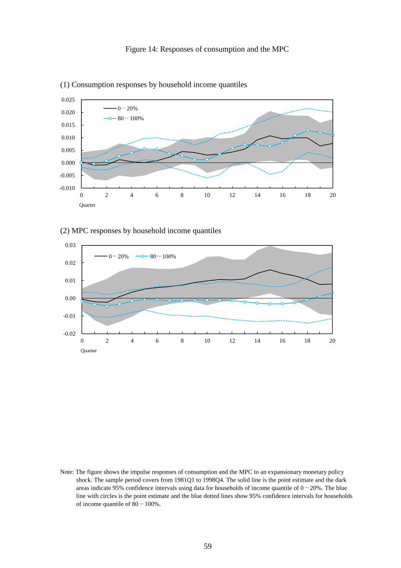
59

Figure 14: Responses of consumption and the MPC

(1) Consumption responses by household income quantiles

(2) MPC responses by household income quantiles

Note: The figure shows the impulse responses of consumption and the MPC to an expansionary monetary policy shock. The sample period covers from 1981Q1 to 1998Q4. The solid line is the point estimate and the dark areas indicate 95% confidence intervals using data for households of income quantile of 0－20%. The blue line with circles is the point estimate and the blue dotted lines show 95% confidence intervals for households of income quantile of 80－100%.

-0.02

-0.01

0.00

0.01

0.02

0.03

0 2 4 6 8 10 12 14 16 18 20

0－20% 80－100%

Quarter

-0.010

-0.005

0.000

0.005

0.010

0.015

0.020

0.025

0 2 4 6 8 10 12 14 16 18 20

0－20%

80－100%

Quarter

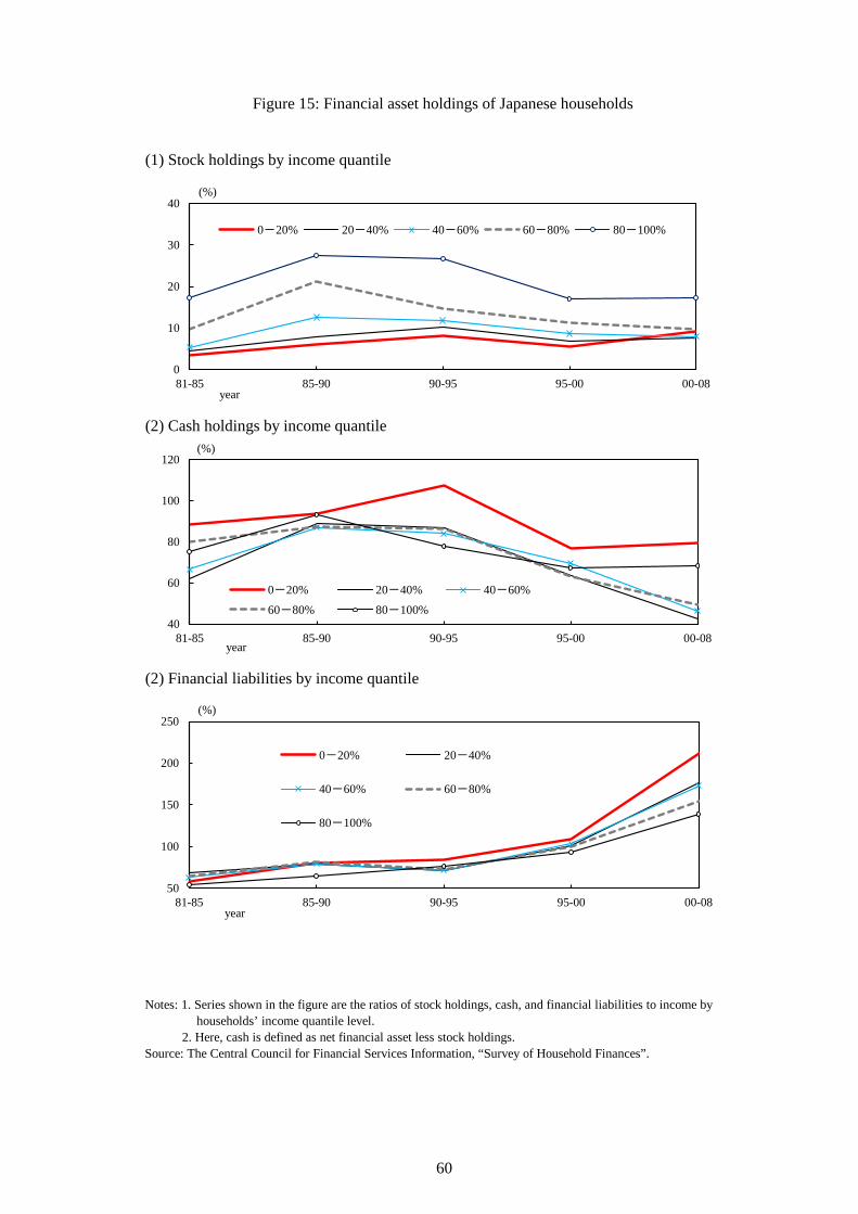
60

Figure 15: Financial asset holdings of Japanese households

(1) Stock holdings by income quantile

(2) Cash holdings by income quantile

(2) Financial liabilities by income quantile

Notes: 1. Series shown in the figure are the ratios of stock holdings, cash, and financial liabilities to income by 　　　 households’ income quantile level.　　　 　2. Here, cash is defined as net financial asset less stock holdings.Source: The Central Council for Financial Services Information, “Survey of Household Finances”.

0

10

20

30

40

81-85 85-90 90-95 95-00 00-08

0－20% 20－40% 40－60% 60－80% 80－100%

(%)

year

40

60

80

100

120

81-85 85-90 90-95 95-00 00-08

0－20% 20－40% 40－60%

60－80% 80－100%

(%)

year

50

100

150

200

250

81-85 85-90 90-95 95-00 00-08

0－20% 20－40%

40－60% 60－80%

80－100%

(%)

year

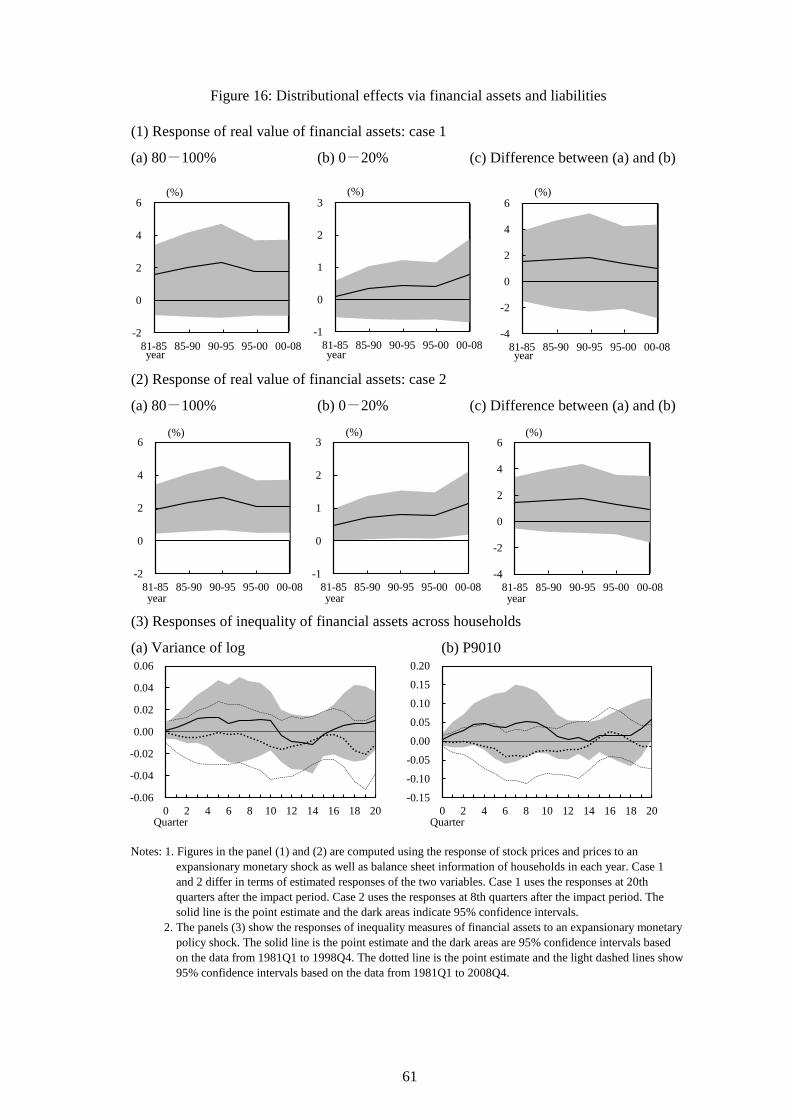
61

Figure 16: Distributional effects via financial assets and liabilities

(1) Response of real value of financial assets: case 1

(2) Response of real value of financial assets: case 2

(3) Responses of inequality of financial assets across households

(a) Variance of log (b) P9010

Notes: 1. Figures in the panel (1) and (2) are computed using the response of stock prices and prices to an expansionary monetary shock as well as balance sheet information of households in each year. Case 1 and 2 differ in terms of estimated responses of the two variables. Case 1 uses the responses at 20th quarters after the impact period. Case 2 uses the responses at 8th quarters after the impact period. The solid line is the point estimate and the dark areas indicate 95% confidence intervals. 2. The panels (3) show the responses of inequality measures of financial assets to an expansionary monetary policy shock. The solid line is the point estimate and the dark areas are 95% confidence intervals based on the data from 1981Q1 to 1998Q4. The dotted line is the point estimate and the light dashed lines show 95% confidence intervals based on the data from 1981Q1 to 2008Q4.

(a) 80－100% (b) 0－20% (c) Difference between (a) and (b)

(a) 80－100% (b) 0－20% (c) Difference between (a) and (b)

-4

-2

0

2

4

6

81-85 85-90 90-95 95-00 00-08

(%)

year

-2

0

2

4

6

81-85 85-90 90-95 95-00 00-08

(%)

year

-2

0

2

4

6

81-85 85-90 90-95 95-00 00-08

(%)

year

-4

-2

0

2

4

6

81-85 85-90 90-95 95-00 00-08

(%)

year

-1

0

1

2

3

81-85 85-90 90-95 95-00 00-08

(%)

year

-0.06

-0.04

-0.02

0.00

0.02

0.04

0.06

0 2 4 6 8 10 12 14 16 18 20

Quarter

-0.15

-0.10

-0.05

0.00

0.05

0.10

0.15

0.20

0 2 4 6 8 10 12 14 16 18 20

Quarter

-1

0

1

2

3

81-85 85-90 90-95 95-00 00-08

(%)

year

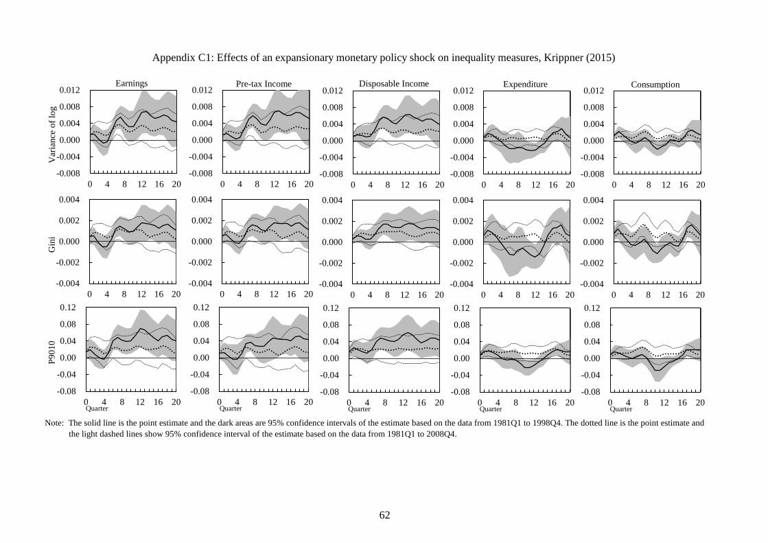
62

Appendix C1: Effects of an expansionary monetary policy shock on inequality measures, Krippner (2015)

Note: The solid line is the point estimate and the dark areas are 95% confidence intervals of the estimate based on the data from 1981Q1 to 1998Q4. The dotted line is the point estimate and the light dashed lines show 95% confidence interval of the estimate based on the data from 1981Q1 to 2008Q4.

-0.008

-0.004

0.000

0.004

0.008

0.012

0 4 8 12 16 20

Earnings

Var

ianc

e of

log

-0.004

-0.002

0.000

0.002

0.004

0 4 8 12 16 20

Gin

i

-0.08

-0.04

0.00

0.04

0.08

0.12

0 4 8 12 16 20Quarter

P901

0

-0.008

-0.004

0.000

0.004

0.008

0.012

0 4 8 12 16 20

Pre-tax Income

-0.004

-0.002

0.000

0.002

0.004

0 4 8 12 16 20

-0.08

-0.04

0.00

0.04

0.08

0.12

0 4 8 12 16 20Quarter

-0.008

-0.004

0.000

0.004

0.008

0.012

0 4 8 12 16 20

Disposable Income

-0.004

-0.002

0.000

0.002

0.004

0 4 8 12 16 20

-0.08

-0.04

0.00

0.04

0.08

0.12

0 4 8 12 16 20Quarter

-0.008

-0.004

0.000

0.004

0.008

0.012

0 4 8 12 16 20

Expenditure

-0.004

-0.002

0.000

0.002

0.004

0 4 8 12 16 20

-0.08

-0.04

0.00

0.04

0.08

0.12

0 4 8 12 16 20Quarter

-0.008

-0.004

0.000

0.004

0.008

0.012

0 4 8 12 16 20

Consumption

-0.004

-0.002

0.000

0.002

0.004

0 4 8 12 16 20

-0.08

-0.04

0.00

0.04

0.08

0.12

0 4 8 12 16 20Quarter

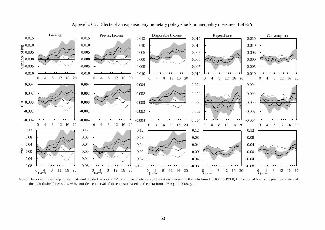
63

Appendix C2: Effects of an expansionary monetary policy shock on inequality measures, JGB-2Y

Note: The solid line is the point estimate and the dark areas are 95% confidence intervals of the estimate based on the data from 1981Q1 to 1998Q4. The dotted line is the point estimate and the light dashed lines show 95% confidence interval of the estimate based on the data from 1981Q1 to 2008Q4.

-0.010

-0.005

0.000

0.005

0.010

0.015

0 4 8 12 16 20

Earnings

Var

ianc

e of

log

-0.004

-0.002

0.000

0.002

0.004

0 4 8 12 16 20

Gin

i

-0.08

-0.04

0.00

0.04

0.08

0.12

0 4 8 12 16 20Quarter

P901

0

-0.010

-0.005

0.000

0.005

0.010

0.015

0 4 8 12 16 20

Pre-tax Income

-0.004

-0.002

0.000

0.002

0.004

0 4 8 12 16 20

-0.08

-0.04

0.00

0.04

0.08

0.12

0 4 8 12 16 20Quarter

-0.010

-0.005

0.000

0.005

0.010

0.015

0 4 8 12 16 20

Disposable Income

-0.004

-0.002

0.000

0.002

0.004

0 4 8 12 16 20

-0.08

-0.04

0.00

0.04

0.08

0.12

0 4 8 12 16 20Quarter

-0.010

-0.005

0.000

0.005

0.010

0.015

0 4 8 12 16 20

Expenditure

-0.004

-0.002

0.000

0.002

0.004

0 4 8 12 16 20

-0.08

-0.04

0.00

0.04

0.08

0.12

0 4 8 12 16 20Quarter

-0.010

-0.005

0.000

0.005

0.010

0.015

0 4 8 12 16 20

Consumption

-0.004

-0.002

0.000

0.002

0.004

0 4 8 12 16 20

-0.08

-0.04

0.00

0.04

0.08

0.12

0 4 8 12 16 20Quarter

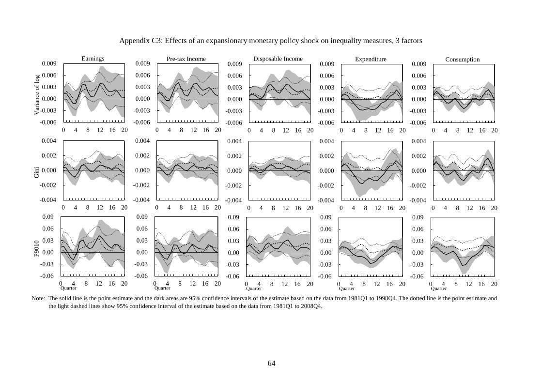
64

Appendix C3: Effects of an expansionary monetary policy shock on inequality measures, 3 factors

Note: The solid line is the point estimate and the dark areas are 95% confidence intervals of the estimate based on the data from 1981Q1 to 1998Q4. The dotted line is the point estimate and the light dashed lines show 95% confidence interval of the estimate based on the data from 1981Q1 to 2008Q4.

-0.006

-0.003

0.000

0.003

0.006

0.009

0 4 8 12 16 20

Earnings

Var

ianc

e of

log

-0.004

-0.002

0.000

0.002

0.004

0 4 8 12 16 20

Gin

i

-0.06

-0.03

0.00

0.03

0.06

0.09

0 4 8 12 16 20Quarter

P901

0

-0.006

-0.003

0.000

0.003

0.006

0.009

0 4 8 12 16 20

Pre-tax Income

-0.004

-0.002

0.000

0.002

0.004

0 4 8 12 16 20

-0.06

-0.03

0.00

0.03

0.06

0.09

0 4 8 12 16 20Quarter

-0.006

-0.003

0.000

0.003

0.006

0.009

0 4 8 12 16 20

Disposable Income

-0.004

-0.002

0.000

0.002

0.004

0 4 8 12 16 20

-0.06

-0.03

0.00

0.03

0.06

0.09

0 4 8 12 16 20Quarter

-0.006

-0.003

0.000

0.003

0.006

0.009

0 4 8 12 16 20

Expenditure

-0.004

-0.002

0.000

0.002

0.004

0 4 8 12 16 20

-0.06

-0.03

0.00

0.03

0.06

0.09

0 4 8 12 16 20Quarter

-0.006

-0.003

0.000

0.003

0.006

0.009

0 4 8 12 16 20

Consumption

-0.004

-0.002

0.000

0.002

0.004

0 4 8 12 16 20

-0.06

-0.03

0.00

0.03

0.06

0.09

0 4 8 12 16 20Quarter

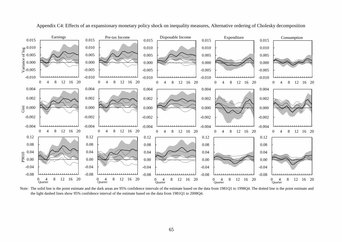
65

Appendix C4: Effects of an expansionary monetary policy shock on inequality measures, Alternative ordering of Cholesky decomposition

Note: The solid line is the point estimate and the dark areas are 95% confidence intervals of the estimate based on the data from 1981Q1 to 1998Q4. The dotted line is the point estimate and the light dashed lines show 95% confidence interval of the estimate based on the data from 1981Q1 to 2008Q4.

-0.010

-0.005

0.000

0.005

0.010

0.015

0 4 8 12 16 20

Earnings

Var

ianc

e of

log

-0.004

-0.002

0.000

0.002

0.004

0 4 8 12 16 20

Gin

i

-0.08

-0.04

0.00

0.04

0.08

0.12

0 4 8 12 16 20Quarter

P901

0

-0.010

-0.005

0.000

0.005

0.010

0.015

0 4 8 12 16 20

Pre-tax Income

-0.004

-0.002

0.000

0.002

0.004

0 4 8 12 16 20

-0.08

-0.04

0.00

0.04

0.08

0.12

0 4 8 12 16 20Quarter

-0.010

-0.005

0.000

0.005

0.010

0.015

0 4 8 12 16 20

Disposable Income

-0.004

-0.002

0.000

0.002

0.004

0 4 8 12 16 20

-0.08

-0.04

0.00

0.04

0.08

0.12

0 4 8 12 16 20Quarter

-0.010

-0.005

0.000

0.005

0.010

0.015

0 4 8 12 16 20

Expenditure

-0.004

-0.002

0.000

0.002

0.004

0 4 8 12 16 20

-0.08

-0.04

0.00

0.04

0.08

0.12

0 4 8 12 16 20Quarter

-0.010

-0.005

0.000

0.005

0.010

0.015

0 4 8 12 16 20

Consumption

-0.004

-0.002

0.000

0.002

0.004

0 4 8 12 16 20

-0.08

-0.04

0.00

0.04

0.08

0.12

0 4 8 12 16 20Quarter