Embed Size (px)
Citation preview

5757 S. University Ave.
Chicago, IL 60637
Main: 773.702.5599
bfi.uchicago.edu
WORKING PAPER · NO. 2018-78
The Propagation of MonetaryPolicy Shocks in a HeterogeneousProduction Economy Ernesto Pasten, Raphael Schoenle, and Michael WeberJULY 2019

The Propagation of Monetary Policy Shocksin a Heterogeneous Production Economy∗
Ernesto Pasten†, Raphael Schoenle‡, and Michael Weber§
This version: July 2019
Abstract
We study the transmission of monetary policy shocks in a model in which realisticheterogeneity in price rigidity interacts with heterogeneity in sectoral size andinput-output linkages, and derive conditions under which these heterogeneitiesgenerate large real effects. Quantitatively, heterogeneity in the frequency of priceadjustment is the most important driver behind large real effects. Heterogeneityin input-output linkages and consumption shares contribute only marginally to realeffects but alter substantially the identity and contribution of the most importantsectors to the transmission of monetary shocks. In the model and data, reducingthe number of sectors decreases monetary non-neutrality with a similar impactresponse of inflation. Hence, the initial response of inflation to monetary shocksis not sufficient to discriminate across models and for the real effects of nominalshocks and ignoring heterogeneous consumption shares and input-output linkagesidentifies the wrong sectors from which the real effects originate.
JEL classification: E30, E32, E52
Keywords: Input-output linkages, multi-sector Calvo model, monetary policy
∗We thank Klaus Adam, Susanto Basu, Carlos Carvalho, Zeno Enders, Xavier Gabaix, Gita Gopinath,Yuriy Gorodnichenko, Bernard Herskovic, Hugo Hopenhayn, Pete Klenow, Alireza Tahbaz-Salehi, HaraldUhlig, and conference and seminar participants at the Annual Inflation Targeting Seminar of the BancoCentral do Brasil, AEA, Banque de France Conference on Price Setting and Inflation, BIS, Brandeis,Cambridge, Carlos III, Cleveland Fed conference on Inflation: Drivers and Dynamics Conference, EEA,Einaudi, FGV Sao Paulo, Konstanz seminar on Monetary Theory, Oxford, St. Louis Fed, SED, Toulouse.Pasten is grateful for the support of the Universite de Toulouse Capitole during his stays in Toulouse.Weber thanks the Fama-Miller Center at the University of Chicago Booth School of Business and theFama Research Fund for financial support. Schoenle and Weber also acknowledge financial support fromthe National Science Foundation under grant 1756997. We also thank Will Cassidy, Seongeun Kim, MattKlepacz and Michael Munsell for excellent research assistance.†Central Bank of Chile and Toulouse School of Economics. e-Mail: [email protected]‡Brandeis University. e-Mail: [email protected].§University of Chicago Booth School of Business and NBER. e-Mail:

I Introduction
Understanding how monetary policy transmits to the real economy and why nominal
shocks have real effects are vital questions in monetary economics. The literature
identified heterogeneity in price rigidities as a central driver behind the real effects of
monetary shocks (see, e.g., Carvalho (2006) and Nakamura and Steinsson (2008)) but
a recent literature suggests other heterogeneities on the production side might also be
important for aggregate fluctuations. Sectors differ in size and different sectors use
different intermediate input mixes to produce output. Gabaix (2011) and Acemoglu,
Carvalho, Ozdaglar, and Tahbaz-Salehi (2012) derive conditions under which these
heterogeneties can generate aggregate fluctuations from idiosyncratic or sectoral real
shocks invalidating the diversification argument of Lucas (1977) and Ozdagli and Weber
(2017) argue production networks shape the stock market response to monetary shocks.
But most of the existing literature has studied how heterogeneities in sector size,
input-output structure, and price stickiness shape aggregate fluctuations in isolation.
In this paper, we present new theoretical insights into the transmission of monetary
policy shocks in an economy in which all three heterogeneities are present and interact
with each other. First, we show real effects of nominal shocks are bigger if the share of
intermediate inputs is high or if sticky-price sectors are important suppliers to the rest
of the economy, to large sectors and to flexible-price sectors on impact, but to sticky
price sectors following the shock.1 Second, the level of disaggregation is central for the
real effects of monetary policy. More granular economies result in larger real effects
with similar price responses on impact. Third, the importance of specific sectors for the
transmission of monetary policy shocks depends on which heterogeneities are present, and
how they interact.
On the quantitative side, our contribution lies in the calibration of a detailed model
of the U.S. economy to study the quantitative importance of the different types of
heterogeneities. We calibrate a 341-sector version of the model to the input-output (I/O)
tables from the Bureau of Economic Analysis (BEA) and the micro-data underlying the
producer price index (PPI) from the Bureau of Labor Statistics (BLS). First, we find
heterogeneity in price stickiness is the main driver of real output effects: It increases
real output effects relative to an economy with homogeneous price stickiness by 70%.
Additionally allowing for heterogeneity in consumption shares or size or both only has a
marginal effect on impact and on cumulative real output effects.
1Some of the results are well known. The dynamic prediction in the network setting is most distinctlynew (see Basu (1995), Huang and Liu (2001, 2004), Shamloo (2010)), and Bouakez, Cardia, and Ruge-Murcia (2014))
2

Second, the choice of disaggregation plays an important role quantitatively. A 341-
sector economy has a 7% (46%) larger cumulative real effect of monetary policy shocks
than a less granular 58-(7-)sector model. However, across choices of aggregation, the
response of inflation to the monetary policy shock is similar on impact and on average
during the first few periods. The large differences in real output effects with similar
impact responses of inflation across different levels of aggregation caution against drawing
inference for the conduct of monetary policy from the initial response of inflation to
monetary policy shocks.
Third, heterogeneity in price rigidity is key in determining which sectors are the
most important contributors to the transmission of monetary shocks. In an economy
with homogeneous price stickiness all sectors respond equally to a common monetary
policy shock independent of their size or I/O structure. Once we introduce different
price stickiness across sectors, sectoral output responses of the 10 most important sectors
increase by 350%. Hence, heterogeneous price stickiness is central for differential sectoral
real effects, but this result does not mean that heterogeneities in sector size and I/O
structure does not matter for sectoral responses. Our baseline economy with all three
heterogeneities present doubles the real effects of the ten most important sectors relative
to the economy with homogeneous sector size and I/O structure and totally scrambles
the identities of the 10 most important, contractionary responses. Thus, even though
heterogeneity in I/O linkages or size only has a marginal effect on the aggregate real
output responses, which sector transmits the monetary policy shock the most depends
crucially on our exact specification of heterogeneities. As we remove heterogeneities, the
distribution of responses also becomes much more compressed.
Notably, heterogeneity in price rigidity also changes the sign of the response for the
least contractionary responses: In fact, the 10 least contractionary sectoral responses are
positive in all combinations that include heterogeneity in price rigidity. As we remove
heterogeneities from the baseline, responses also become more compressed and smaller –
but only negative when price rigidity becomes homogeneous. The flip in sign is due to
the fact that the 10 least contractionary, expansionary responses are concentrated in the
most flexible sectors. These sectors can gain market share from lowering their relative
prices more quickly than stickier-price sectors.
Taken together, these results show (i) Heterogeneous price stickiness is the central
force for the real effects of nominal shocks; heterogeneity in intermediate input usage and
in the I/O structure is less important; (ii) disaggregation matters for the real effects of
monetary policy shocks but leaves the impact response of inflation largely unchanged;
(iii) price stickiness that differs across sectors changes the identity and importance of the
3

most important sectors for the transmission of monetary shocks; (iv) heterogeneous sector
size and I/O structures further change the identity of the most important sectors for the
real effects of monetary shocks and increase their importance, and hence, the effective
granularity of the economy increases.
What mechanisms drive these results? In the model, firms set prices as a markup
over a weighted average of future marginal costs. We identify four distinct channels
through which I/O linkages and the heterogeneities of sector size and price stickiness
affect the marginal-cost process. First, marginal costs of final-goods producers depend
directly on the sector-specific input price index. Second, sector-specific wages depend
indirectly on I/O linkages because the optimal mix of inputs depends on the relative price
of intermediate inputs and labor. Third and fourth, the heterogeneities across sectors in
total production, value-added, and intermediate inputs create wedges between sectoral
participation in total output, production, and total GDP that feed back into marginal
costs. These channels interact in shaping the response to nominal shocks in a very intuitive
way: How important is the output of a given sector for final-goods production? How
flexible are the output prices of the goods the sector uses in production? How important
is the sector as a producer for total consumption?
We develop further, analytical intuition for the interaction of the three heterogeneities
in a simplified model. In this economy, we gradually add each heterogeneity, and prove
results analytically when possible. We start with an economy that features I/O linkages
that can be homogeneous or heterogeneous across sectors. Key to this step is that price
rigidity is homogeneous across sectors, and sectoral participation in GDP equals sectoral
participation in total production. I/O linkages per se amplify the real effects of monetary
policy, as in Nakamura and Steinsson (2008). However, heterogeneity in consumption
shares and I/O linkages does not matter, because sectoral production and consumption
shares do not produce wedges.
We then add heterogeneity in Calvo parameters. This addition generates a hump-
shaped response in consumption, because flexible-price firms compete with sticky-price
firms. Firms with flexible prices adjust prices in a staggered fashion and by less on impact
than in a model with homogeneous Calvo rates across sectors. The dispersion of price
stickiness amplifies cumulative real effects following an identical impact of consumption
as in Carvalho (2006), Carvalho and Schwartzman (2015), and Alvarez et al. (2016).
Heterogeneity in I/O linkages and consumption shares does not affect the impact response
relative to an economy with homogeneous price stickiness and also does not have any
systematic effect following the impact response.
Last, we allow for fully unrestricted heterogeneity in sector weights in GDP and in I/O
4

linkages. This additional degree of heterogeneity results in wedges between consumption
prices and sectoral intermediate input prices, which influence sectoral marginal costs.
Heterogeneity in I/O linkages can amplify or dampen the output response. For example,
the economy may resemble more of a flexible-price economy or a sticky-price economy,
depending on the interaction of sector size, the importance of sectors as suppliers to
other sectors, and sectoral price stickiness. We characterize the interactions and their
influence on real effects of monetary policy by three relations: (i) first-order out-degrees
to sector size, (ii) first-order outdegrees adjusted by average flexibility to sector size, and
(iii) covariances between sectoral linkages and size with price stickiness.
A. Literature review
Our paper contributes new insights to the literature on the transmission of monetary
policy shocks in a network economy. Basu (1995) shows a roundabout production
structure can magnify the importance of price rigidities through its effect on marginal
costs, and results in larger welfare losses of demand-driven business cycles. Huang
and Liu (2001, 2004) study the persistence of monetary shocks in a multi-sector model
with roundabout production and fixed contract length. Aggregate output becomes
more persistent in the their setup the higher the number of production stages and
the share of intermediates. Their work theoretically shows that intermediate inputs
amplify the importance of rigid prices with no impact on wage stickiness. Nakamura
and Steinsson (2010) develop a multi-sector menu-cost model and show in a calibration of
a six-sector version that heterogeneity in price stickiness together with I/O linkages can
explain persistent real effects of nominal shocks with moderate degrees of price stickiness.
Carvalho and Lee (2011) show a multi-sector Calvo model with intermediate inputs can
reconcile why firms adjust more quickly to idiosyncratic shocks than to aggregate shocks
(see also Boivin et al. (2009) and Shamloo (2010)). Bouakez, Cardia, and Ruge-Murcia
(2014) estimate a multi-sector Calvo model with production networks using aggregate
and sectoral data, and find evidence of heterogeneity in frequencies of price adjustments
across sectors.
We contribute several new insights to this literature. Our most important
quantitative innovation is to study the importance of networks on the propagation of
nominal shocks in a detailed, 341-sector calibration of the U.S. economy. Second, we show
both theoretically and quantitatively that reducing the number of sectors in our model
decreases monetary non-neutrality. By contrast, across calibrations the impact response
of inflation is similar across aggregation choices, and hence is not a sufficient statistic for
5

monetary non-neutrality. Finally, we point out a new identity effect: Heterogeneity in
price rigidity is key in determining which sectors are the most important contributors to
the transmission of monetary shocks but heterogeneity in sector size and I/O structure can
change the sectoral identify substantially, and makes important contributors even more
important and down-weighs the contribution of less important sectors. A few sectors with
flexible prices can also increase their output following a contractionary shock, given their
fall in relative price.
A high degree of specialization is a general, key feature of modern production
economies. Gabaix (2011) and Acemoglu et al. (2012) show theoretically the network
structure and the firm-size distribution are potentially important propagation mechanisms
for aggregate fluctuations originating from firm and industry shocks. Acemoglu, Akcigit,
and Kerr (2015) and Barrot and Sauvagnat (2016) show empirical evidence for the
propagation of idiosyncratic supply shocks through the I/O structure. Carvalho (2014)
provides an overview of this fast-growing literature. Idiosyncratic shocks propagate
through changes in prices. In a companion paper (see Pasten, Schoenle, and Weber
(2018)), we study how price rigidities affect the importance of idiosyncratic shocks as an
origin of aggregate fluctuations.
Other recent applications of production networks in different areas of macroeconomics
include Bigio and Lao (2017) who study the amplification of financial frictions through
production networks, and Ozdagli and Weber (2017), who empirically show I/O linkages
are a key propagation channel of monetary policy to the stock market. Additionally,
Kelly, Lustig, and Van Nieuwerburgh (2013) study the joined dynamics of the firm-size
distribution and stock return volatilities. Herskovic, Kelly, Lustig, and Van Nieuwerburgh
(2016) and Herskovic (2018) study asset-pricing implications of production networks.
II Model
This section presents our full blown New Keynesian model. We highlight in particular
how heterogeneities in price rigidities, sectoral size, and I/O linkages enter the model.
A. Firms
A continuum of monopolistically competitive firms j operates in different sectors. We
index firms by their sector, k = 1, ..., K, and by j ∈ [0, 1]. The set of consumption
goods is partitioned into a sequence of subsets =kKk=1 with measure nkKk=1 such that∑Kk=1 nk = 1.
6
The first, real heterogeneity – heterogeneity in sectoral I/O linkages – enters via the
production function of firm j in sector k
Ykjt = L1−δkjt Z
δkjt, (1)
where Lkjt is labor and Zkjt is an aggregator of intermediate inputs
Zkjt ≡
[K∑r=1
ω1η
krZkjt (r)1− 1η
] ηη−1
. (2)
Here, Zkjt (r) denotes the intermediate input use by firm j in sector k in period t. The
aggregator weights ωkrk,r satisfy∑K
r=1 ωkr = 1 for all sectors k. We allow these weights
to differ across sectors, which is a central ingredient of our analysis.
In turn, Zkjt (r) is an aggregator of goods produced in sector r,
Zkjt (r) ≡[n−1/θr
∫=rZkjt (r, j′)
1− 1θ dj′
] θθ−1
. (3)
Zkjt (r, j′) is the amount of goods firm j′ in sector r produces that firm k, j uses as input.
Demand for intermediate inputs Zkjt (r) and Zkjt (r, j′) is given by the following
demand equations
Zkjt (r) = ωkr
(PrtPkt
)−ηZkjt,
Zkjt (r, j′) =1
nr
(Prj′tPrt
)−θZkjt (r) .
Prj′t is the price firm j′ in sector r charges, Prt is a sectoral price index, and Pkt is
an input-price index; we define both price indices below. In steady state, all prices are
identical, and ωkrKr=1 is the share of costs that firm k, j spends on inputs from sector r
and, hence, equals cell k, r in the I/O Tables (see online appendix). We refer to ωkrKr=1
as “I/O linkages.” As a result, in steady state, all nr firms in sector r share the demand
of firm k, j for goods that sector r produces equally.
Away from steady state, a gap exists between the price index of sector r, Prt, and
the input price index, Pkt, that is relevant for firms in sector k. It distorts the share of
sector r in the costs of firms in sector k. Similarly, price dispersion across firms within
sector r determines the dispersion of demand of firms in sector k for goods in sector r.
7

Price indices relevant for the demand of intermediate inputs across sectors are defined as
Pkt =
[K∑r=1
ωkrP1−ηrt
] 11−η
,
Prt =
[1
nr
∫=rP 1−θrj′t dj
′] 1
1−θ
.
Our second heterogeneity – heterogeneity of price rigidity – originates from our assumption
about price setting. Firms set prices as in Calvo (1983), but we allow for differences in
Calvo rates across sectors, αkKk=1. That is, the objective of firm j, k is given
maxPkjt
Et∞∑s=0
Qt,t+sαsk [PkjtYkjt+s −MCkt+sYkjt+s] , (4)
where MCkt = 11−δ
(δ
1−δ
)−δW 1−δkt
(P kt
)δare marginal costs after imposing the optimal mix
of labor and intermediate inputs
δWktLkjt = (1− δ)P kt Zkjt. (5)
The optimal pricing problem takes the standard form
∞∑s=0
Qt,t+sαskYkjt+s
[P ∗kt −
θ
θ − 1MCkjt+s
]= 0. (6)
Ykjt+s is the total output of firm k, j at period t+s, Qt,t+s is the stochastic discount factor
between period t and t+ s, and θ is the elasticity of substitution within sector.
The optimal price for all adjusting firms within a given sector is identical, P ∗kt, allowing
simple aggregation. Hence, the law of motion for sectoral prices is
Pkt =[(1− αk)P ∗1−θkt + αkP
1−θkt−1
] 11−θ ∀k. (7)
B. Households
A large number of infinitely lived households exist. Households have a love for variety,
and derive utility from consumption and leisure. Households supply all different types of
labor. The representative household has additively separable utility in consumption and
8

leisure and maximizes
maxE0
∞∑t=0
βt
(C1−σt − 1
1− σ−
K∑k=1
∫=kgkL1+ϕkjt
1 + ϕdj
)(8)
subject to
PCtCt =K∑k=1
Wkt
∫=kLkjtdj +
K∑k=1
Πkt + It−1Bt−1 −Bt. (9)
The budget constraint states nominal expenditure equals nominal household income. Ct
and PCt are aggregate consumption and prices, which we define below. Lkjt and Wkt
are labor employed and wages paid by firm j in sector k. Households own firms and
receive net income, Πkt, as dividends. Bonds, Bt, pay a nominal gross interest rate of
It−1. gkKk=1 are parameters that we choose to ensure a symmetric steady state across
all firms.
Aggregate consumption is
Ct ≡
[K∑k=1
ω1η
ckC1− 1
η
kt
] ηη−1
, (10)
where Ckt is the aggregation of sectoral consumption
Ckt ≡[n−1/θk
∫=kC
1− 1θ
kjt dj
] θθ−1
. (11)
Ckjt is the consumption of goods that firm j in sector k produces.
We allow the elasticity of substitution across sectors η to differ from the elasticity
of substitution within sectors θ. We also allow the consumption weights ωck to differ
across sectors, which is the third heterogeneity across sectors in our model. The weights
satisfy∑K
k=1 ωck = 1.
Households’ demand for sectoral goods Ckt and firm goods Ckjt is
Ckt = ωck
(PktPCt
)−ηCt,
Ckjt =1
nk
(PkjtPkt
)−θCkt.
We solve in the online appendix for the steady state of the economy. We show
the consumption weights ωckKr=1 determine the steady-state shares of sectors in total
consumption (or value-added production). In the following, we refer to ωckKr=1 as
9

“consumption shares.” Heterogeneity in sectoral size enters through these shares. Away
from steady state, a gap between sectoral prices, PrtKr=1, and aggregate consumption
prices, PCt, distorts the share of sectors in aggregate consumption.2
The consumption price index PCt is given by
PCt =
[K∑k=1
ωckP1−ηkt
] 11−η
, (12)
and sectoral prices follow
Pkt =
[1
nk
∫=kP 1−θkjt dj
] 11−θ
. (13)
C. Monetary policy
The monetary authority sets the short-term nominal interest rate, It, according to a
Taylor rule
It =1
β
(PCtPCt−1
)φπ (CtC
)φyeµt . (14)
µt is a monetary shock following an AR(1) process with persistence ρµ. Thus, monetary
policy reacts to aggregate consumption inflation and aggregate consumption.
In our quantitative exercises, we also study economies with interest rates smoothing
similar to Coibion and Gorodnichenko (2012).
D. Equilibrium conditions and definitions
Bt = 0, (15)
Lkt =
∫=kLkjtdj, (16)
Wt ≡K∑k=1
nkWkt, (17)
Lt ≡K∑k=1
Lkt, (18)
2The measure of firms in sector k, nk, and the consumption shares are related in equilibrium (seeonline appendix).
10

Ykjt = Ckjt +K∑k′=1
∫=k′
Zk′j′t (k, j) dj′. (19)
Equation (15) is the market-clearing condition in bond markets. Equation (16)
defines aggregate labor in sector k. Equations (17) and (18) give aggregate wage (which is
a weighted average of sectoral wages) and aggregate labor (which linearly sums up hours
worked in all sectors). Equation (19) is Walras’ law for the output of firm j in sector k.
III Heterogeneities and Marginal Costs
The dynamic behavior of marginal costs is crucial for understanding the response of the
economy to a monetary policy shock. This section develops intuition for the effects of
heterogeneity in price stickiness, I/O linkages, and sectoral size on marginal costs, and
the real effects of monetary policy in a log-linearized system that we detail in the online
appendix. In the following, small letters denote log deviations from steady state. We
focus on the role of heterogeneity in I/O linkages. Our main, analytical propositions in
the next section, however, do not require reading this section first.
We highlight how I/O linkages affect marginal costs and demand through four distinct
channels. In particular, a new wedge emerges that drives marginal costs: I/O linkages
create a difference between the aggregate consumption price index and intermediate input
price indices that affects marginal costs.
The reduced-form system that embeds marginal costs has K + 1 equations and
unknowns: value-added production ct and K sectoral prices pktk=1. The first equation
is
σEt [ct+1]− (σ + φc) ct + Et [pct+1]− (1 + φπ) pct + φπpct−1 = µt, (20)
which is a combination of the household Euler equation and the Taylor rule. The equation
describes how variations in value-added production, ct, and aggregate consumption prices,
pct, respond to the monetary policy shock, µt.
Note pct is given by
pct =K∑k=1
ωckpkt. (21)
In addition, K equations governing sectoral prices
βEt [pkt+1]− (1 + β) pkt + pkt−1 = κk (pkt −mckt) , (22)
complete the system, where κk ≡ (1− αk) (1− αkβ) /αk measures the degree of price
11

flexibility.
A. The effect of I/O linkages on marginal cost
Here, we show that I/O linkages crucially affect marginal costs. We distinguish between
the use of intermediate inputs per se (i.e., δ > 0) and heterogeneous usage of intermediate
inputs across sectors (i.e., ωkr 6= ωk′r ∀k,∀k′ 6= k, and ∀r). Although our focus is on I/O
linkages, heterogeneity in sectoral size ωck and in pricing frictions is also present through
κk. We first derive how I/O linkages affect several intermediate, key variables.
First, I/O linkages affect the measure of sectors, nkKk=1. The measure reflects the
weighted average of the consumption share of sector k, ωck, and the importance of sector
k as a supplier to the economy, ζk
nk = (1− ψ)ωck + ψζk, (23)
where
ζk ≡K∑k′=1
nk′tωk′k. (24)
We refer to ζk as the “outdegree” of sector k, analogous to Acemoglu et al. (2012). The
outdegree of sector k is the weighted sum of intermediate input use from sector k by all
other sectors ωk′k, with weights nk′t. In steady state, all firms are identical and we can
interpret nk as the size of sector k.
Without intermediate inputs (δ = 0), ψ ≡ δ (θ − 1) /θ = 0, and only consumption
shares determine sector size. By contrast, when firms use intermediate inputs for
production (δ > 0), heterogeneity in I/O linkages results in additional heterogeneities
in sector size. The outdegree of sector k is higher when sector k is a supplier to many
sectors or is a supplier of large sectors.
The vector ℵ of sector sizes nkKk=1 solves
ℵ = (1− ψ) [IK − ψΩ′]−1
ΩC , (25)
where IK is the identity matrix of dimension K, Ω is the I/O matrix in steady state with
elements ωkk′, and ΩC is the vector of consumption shares, ωck.Second, heterogeneity in I/O linkages implies each sector faces a different intermediate
input price index
pkt =K∑k′=1
ωkk′pk′t. (26)
12

In particular, the sector-k intermediate input price index responds more to variation in
the prices of another sector k′ when that sector is a large supplier to sector k.
A.1 Direct effect on sectoral marginal costs
With intermediate inputs in production (δ > 0), sectoral marginal costs are a weighted
average of sectoral wages, but also sectoral intermediate input price indices
mckt = (1− δ)wkt + δpkt. (27)
The sectoral intermediate input price index, pkt, reflects heterogeneity in I/O linkages.
All else equal, an increase in the price of another sector k′ implies higher costs of the
intermediate input mix. Heterogeneity in I/O linkages allows this channel to differ across
sectors.
A.2 Indirect effect through sectoral wages
I/O linkages also affect sectoral wages wkt indirectly because the efficient mix of labor
and intermediate inputs in equation (5) depends on relative input prices. The production
function implicitly defines sectoral labor demand for a given level of production ykt
ykt = lkt + δ (wkt −pkt) . (28)
In a model without I/O linkages (δ = 0), sectoral labor demand is inelastic after
conditioning on sectoral production ykt. Here, I/O linkages (δ > 0) imply labor demand
depends negatively on wages, because higher wages lead firms to substitute labor for
intermediate inputs.
Combining the production function and sectoral labor supply yields
wkt =1
1 + δϕ[ϕykt + σct + δϕ (pkt − pct)] + pct. (29)
Thus, the optimal choice implies a wedge between sectoral intermediate input prices and
aggregate consumption prices, (pkt − pct).What is the role of this wedge? In a model without I/O linkages (δ = 0), wages
respond one to one to variations in aggregate consumption prices pct through their effect
on labor supply. An increase in sector k′ prices positively affects wages in sector k. The
relevant elasticity is tied to the consumption share of sector k′, ωck′ . This effect is captured
by the last term of equation (29).
13

In the presence of I/O linkages (δ > 0), this last term continues to affect wages.
However, the wedge (pkt − pct) now additionally comes into play: An increase in sector
k′ prices has an additional, positive effect on sector k wages when the share of sector k′
as a supplier of sector k is larger than its consumption share, that is, when ωkk′ > ωck′ .
Intuitively, if sector k′ is a large supplier to sector k, a positive variation in pk′t has a
larger effect on increasing the cost of intermediate inputs for firms in sector k. As a result,
firms in sector k increase the demand for labor, and sector k wages go up.
A.3 Effect on sectoral demand
Next, we show I/O linkages can heterogeneously affect how variations in aggregate demand
yt transmit into sectoral demand, yktKk=1. This follows because sectoral demand is given
by
ykt = yt − η [pkt − (1− ψ) pct − ψpt] , (30)
where
pt ≡K∑k=1
nkpkt. (31)
Sectoral demand depends on the sectoral relative price, pkt, relative to a weighted
average of aggregate consumption prices, pct, and an “average sector-relevant” price, pt.
The latter weights sector-relevant aggregate prices by the size of sectors. We can write it
as
pt =K∑k=1
ζkpkt, (32)
that is, the sum of variations in sectoral prices weighted by their outdegrees ζkKk=1.
Following an increase in prices of another sector k′, the share of sector k in total
demand increases in the outdegree of that other sector. This increase is stronger than the
increase in an economy without intermediate inputs if that sector is a big supplier in the
whole economy: ζk′ > ωck′ .
A.4 Effect on total demand
Finally, aggregate demand, yt, also interacts with heterogeneity in I/O linkages.
Aggregating Walras’ law across all industries yields
yt = (1− ψ) ct + ψzt, (33)
14

where zt is the total amount of intermediate inputs. The pure presence of intermediate
inputs creates a wedge between total production, yt, and value-added production, ct. The
dynamics of zt around the steady state depend on the heterogeneity in I/O linkages across
sectors.
We solve for zt, combining Walras’ law, the aggregate production function, aggregate
labor supply, and the aggregation of efficient mixes between labor and intermediate inputs,
zt =[(1 + ϕ) (1− ψ) + σ (1− δ)] ct − (1− δ) (pt − pct)
(1− ψ) + ϕ (δ − ψ). (34)
In an economy with no I/O linkages (δ = 0, ψ = 0), output equals consumption,
yt = ct. With intermediate inputs (δ > 0), zt varies positively with ct: More value-added
production requires more intermediate inputs. This channel shows up as the first term in
the numerator of equation (34). At the same time, an increase in prices of a given sector
k′ has a negative effect on zt when that sector is central in the economy. This second
effect is captured by the wedge (pt − pct), the second term in the numerator of equation
(34), equivalent to the condition that sectors are relatively more central than their GDP
share implies: ζk′ > ωck′ . Then, an increase in prices of big suppliers in the economy
results in higher prices for intermediate inputs for many sectors and/ or bigger sectors.
These sectors then substitute intermediate inputs for labor, and the aggregate demand
for intermediate inputs decreases.
To simplify exposition, we write the relationship between yt and ct as
yt = (1 + ψΓc) ct − ψΓp (pt − pct) , (35)
where Γc ≡ (1−δ)(σ+ϕ)(1−ψ)+ϕ(δ−ψ)
,Γp ≡ 1−δ(1−ψ)+ϕ(δ−ψ)
.
B. Overall solution for log-linearized marginal costs
We combine equations that we derived in the previous subsections to express marginalcosts in terms of value-added production and sectoral prices
mckt =
[1 +
(1− δ)ϕη1 + δϕ
]pct + δ
1 + ϕ
1 + δϕ(pkt − pct) + (1− δ) ϕψ (η − Γp)
1 + δϕ(pt − pct) (36)
− (1− δ)ϕη1 + δϕ
pkt +1− δ
1 + δϕ[σ + ϕ (1 + ψΓc)] ct.
By contrast, in an otherwise identical economy with no I/O linkages (δ = 0), marginal
15

costs are given by
mcδ=0kt = (1 + ϕη) pct − ϕηpkt + (σ + ϕ) ct. (37)
In such an economy, an increase in prices of other sectors, pk′t, increases marginal costs.
This effect uniformly depends on elasticities 1 +ϕη, and specifically, on the heterogeneity
in consumption shares ωck′ .
In our setting, new effects arise. The first line of equation (36) shows how sectoral
prices affect sectoral marginal costs in an economy with I/O linkages (δ > 0). The effect
of prices of other sectors on sector k marginal costs – contained in aggregate consumption
prices via the first term – continues to be present, but is now mitigated because 1 +
(1 − δ)ϕη/(1 + δϕ) < (1 + ϕη). At the same time, I/O linkages create new channels. In
particular, prices of another sector pk′t have a stronger effect on mckt if (i) sector k′ is a
big supplier to sector k; that is, ωkk′ > ωck′ so that the wedge (pkt − pct) > 0 (second
term on the right-hand side of equation (36)); and (ii) sector k′ is a big supplier in the
whole economy; that is, ζk′ > ωck′ so that the wedge (pt − pct) > 0 (third term on the
right-hand side of equation (36)). The overall direct effect of variations in pk′t on mckt is
(1− δ) [1 + (1− ψ)ϕη + ψϕΓp]
1 + δϕωck′ + δ
1 + ϕ
1 + δϕωkk′ + (1− δ) ϕψ (η − Γp)
1 + δϕζk′ . (38)
The last two terms of equation (36) are standard. The fourth term on the right-hand
side of equation (36) shows sector k marginal costs decrease in sector k prices. The
demand for sectoral output is a decreasing function of its price, and hence, wages in
sector k. The fifth term on the right-hand side of equation (36) shows marginal costs
increase in value-added production ct.
IV Theoretical Results
Here, we present new, closed-form results for the response of inflation and consumption
to a monetary policy shock. In doing so, we benchmark our economy with heterogeneity
in price rigidity against an economy in which prices are homogeneously rigid. We
highlight how the I/O structure interacts with the pricing frictions and heterogeneity
in sectoral size and shapes our results. We show that the identity effect – which
sector contributes the most to monetary transmission – can be crucially affected by the
interaction of heterogeneities. Also, the level of aggregation can be key for the degree of
monetary non-neutrality. The latter two insights provide important guidance for monetary
policymakers trying to correctly assess the most important sectors for the transmission of
16

monetary policy shocks to output and inflation.
A. Monetary non-neutrality in the simplified model
We start by introducing three assumptions that allow us to obtain results in closed form.
First, household utility is log in consumption, σ = 1, and linear in leisure, ϕ = 0, such
that
wt = ct + pct. (39)
Second, the central bank targets a given level mt of nominal aggregate demand,
mt = ct + pct, (40)
where pct ≡K∑k=1
ωckpkt.
Third, firms fully discount the future when adjusting prices (β = 0), so
p∗kt = mckt. (41)
Combining all these equations with the sectoral aggregation of prices
pkt = (1− αk) p∗kt + αkpkt−1, (42)
yields
pkt = (1− αk) [(1− δ)mt + δpkt] + αkpkt−1 for k = 1, ..., K (43)
with solution for the sectoral vector of prices
pt = (1− δ)∞∑τ=0
([I− δ (I− A) Ω]−1A
)τ[I− δ (I− A) Ω]−1 (I− A) ιmt−τ . (44)
where Ω denotes the matrix of I/O weights, A the diagonal matrix of αk, and ι a unit
vector of suitable dimension.
In the following, we use equations (40) and (43) to build intuition on the determinants
of monetary non-neutrality in the model. In particular, we assume the economy is in
steady state when a permanent monetary shock hits at period t∗ such that mt = m for all
t ≥ t∗ and mt = 0 for all t < t∗. We focus on characterizing the response of the aggregate
consumption price index pct to the shock in three cases. In this simplified model, the
17

aggregate price response is a sufficient statistic for the real output response.
First, we consider the case in which price stickiness is homogeneous across sectors.
This assumption sets up a useful benchmark for the following cases that feature
heterogeneity in price stickiness, as well as our subsequent discussion of the effect of
sectoral aggregation. At the same time, we are not placing any restrictions on the sectoral
GDP shares ωck and the I/O structure ωkk′ yet.
Proposition 1 When price stickiness is homogeneous across sectors, αk = α for all k,
the response of aggregate consumption prices to a permanent monetary policy shock is
pct (α) =
[1−
(α
1− δ (1− α)
)t−t∗+1]m for t ≥ t∗, (45)
such that
(1) pct (α) is decreasing in δ for any t ≥ t∗, and
(2) heterogeneity of consumption shares ωckKk=1 and I/O linkages ωkk′Kk,k′=1 is
irrelevant for the response of aggregate consumption prices to the monetary shock.
Proof. See online appendix.
The proposition presents two insights. First, the stickiness of marginal costs increases
in δ; hence, the responsiveness of the aggregate consumption price index to the monetary
policy shock decreases in δ. As a result, a lesser price response means stronger monetary
non-neutrality. This result mimics the insights of the network multiplier in Basu (1995).
Second, heterogeneity of consumption shares and I/O linkages are irrelevant for monetary
non-neutrality with homogeneous price stickiness across sectors.
What happens if we allow for heterogeneity in price stickiness? The next proposition
shows heterogeneity of price rigidity amplifies (mitigates) the response of output (prices)
in all periods except upon impact – when it has no effect. This result follows, as a first
step, from a simplified I/O structure. We fully relax this assumption in the subsequent
proposition.
Proposition 2 In an economy in which price stickiness is heterogeneous across sectors
and I/O linkages are identical to consumption shares, ωkk′ = ωck′ for all k, k′, the response
of aggregate consumption prices to a permanent monetary policy shock is
pct = 1−δ1−δ(1−α)
(1−
K∑k=1
ωckαt−t∗+1k
)m+ δ
1−δ(1−α)
t−t∗∑τ=1
(K∑k=1
ωckατk (1− αk)
)pct−τ if t ≥ t∗,
(46)
18

where α ≡K∑k=1
ωckαk, such that
(1) The sectoral heterogeneity of price stickiness and consumption shares are
irrelevant for the response of output to the monetary shock on impact.
(2) pct ≤ pct (α) for t > t∗. The response of the aggregate consumption prices
for t ≥ t∗ is weakly decreasing in the dispersion of price stickiness, and depends on
heterogeneities.
Proof. See online appendix
Proposition 2 studies a simplified steady-state network economy in which sectoral
output is used in equal proportions by consumers and other sectors. In this economy,
sectoral heterogeneity in price stickiness amplifies monetary non-neutrality, as in Carvalho
(2006) and Carvalho and Schwartzman (2015). In particular, sectoral heterogeneity
of price stickiness does not affect the impact response, but increases the persistence
of monetary non-neutrality. However, in an economy in which firms set prices in a
forward-looking manner (β > 0), the increased persistence of monetary non-neutrality
would also imply stronger monetary non-neutrality on impact.
What happens in the fully unrestricted case when price stickiness, sectoral size, and
I/O linkages are heterogeneous across sectors?
Proposition 3 Let pct denote the response of the aggregate consumption price index to apermanent monetary shock in an economy with no restrictions on the sectoral heterogeneityof price stickiness αk, sectoral size ωck, and I/O linkages ωkk′. In this economy,
pct = (1− δ)
(1−
K∑k=1
ωckαt−t∗+1k
)m+ δ
t−t∗∑τ=0
K∑k=1
(K∑k′=1
ωck′ατk′ (1− αk′)ωk′k
)pkt−τ for t ≥ t∗,
(47)
with pkt−τ = 0 if t < t∗ such that
(1) The response of pct is weaker on impact than in Proposition 2, when uk ≡∑Kk′=1 ωck′ (1− αk′)ωk′k > (1− α)ωck for the sectors with the stickiest prices.
(2) The response of pct for t > t∗ is more persistent than in Proposition 2, when
for sectors with the stickiest prices, either of the following conditions hold: (i) ωk ≡1K
∑Kk′=1 ωk′k > ωck, (ii) uk > (1− α)ωck, (iii) COV (ωck′α
τk′ (1− αk′) , ωk′k) > 0.
Proof. See online appendix.
The fully unrestricted interaction creates an even richer transmission of monetary
policy shocks. In doing so, the exact interaction of nominal and real heterogeneities is
crucial for understanding the effects of a monetary shock on output and prices. The
implications we find are completely new to the literature.
19

First, upon impact, the price effect is weaker – and hence monetary non-neutrality
larger – than under the restricted heterogeneity of I/O linkages in Proposition 2. This
effect happens when the largest sectors with the stickiest prices are also important
suppliers to the largest, most flexible sectors. Second, in subsequent periods, aggregate
price changes become more persistent given the three conditions in the second part of the
proposition. In conjunction with the first result, this increased persistence means more
persistence and larger monetary non-neutrality than under restricted heterogeneity.3
In particular, a corollary of these results is a novel identity effect: The extent to
which a sector transmits monetary policy shocks depends on the exact interaction of
heterogeneity in pricing frictions and heterogeneity in sectoral size and I/O linkages. The
following corollaries summarize the contribution of each sector to the path of aggregate
prices, first upon impact only, and then for all subsequent periods.
Corollary 1 Upon impact, each sectoral contribution to the path of aggregate prices is
given
(1) independently of heterogeneity in I/O linkages under homogeneous price rigidity,
by [1−
((1− δ)(1− α)
1− δ (1− α)
)]ωckm, and (48)
(2) by a function of heterogeneities under heterogeneous price rigidity,
e′kΩc (1− δ) [I− δ (I− A) Ω]−1 (I− A) ιm, (49)
where ek is the kth basis vector, Ω the matrix of I/O weights, Ωc the vector of
consumption weights, A the diagonal matrix of αk, and ι a unit vector. In the special
case of ωck′ = ωkk′, the kth element equals[1−
((1−δ)(1−αk)
1−δ(1−α)
)]ωckm.
Corollary 2 In subsequent periods, t > t∗, each sectoral contribution to the path of
aggregate prices is given
(1) independently of heterogeneity in I/O linkages under homogeneous price rigidity,[1−
(α
1− δ (1− α)
)t−t∗+1]ωckm, and (50)
3Note we have left a contemporaneous term in the second term on the right-hand side of the propositionto make it more comparable to Proposition 2. The online appendix contains an explicit solution in termsof parameters and the monetary shock only.
20

(2) by the interaction of the heterogeneities under heterogeneous price rigidity,
e′kΩc (1− δ)
t−t∗∑τ=0
([I− δ (I− A) Ω]−1A
)τ[I− δ (I− A) Ω]−1 (I− A) ιmt−τ , (51)
where ek is the kth basis vector, Ω the matrix of input-output weights, Ωc the vector
of consumption weights and A the diagonal matrix of αk.
Proof. See online appendix.
The importance of each sector to the monetary transmission mechanism crucially
depends on the interaction of heterogeneities. Timing also plays an important role,
whether we consider the impact response, or subsequent responses. The ranking of
importance across the different cases can clearly change. For example, sectors that are
important upon impact may be less important later on. Similarly, heterogeneity in I/O
linkages can influence the importance of a sector. Ultimately, the extent to which the
interaction of heterogeneities can affect the relative importance of sectors for aggregate
fluctuations is a quantitative question.
We have not placed any restrictions on the total effect of monetary policy. Monetary
policy shocks could easily generate the same real effects under different assumptions about
which heterogeneities are present, whereas sectors are differently important in generating
the same real effects. For example, consider a two-sector economy that generates a
particular path of real output and prices following a monetary policy shocks. Now, if
we simply flip all parameter values for the two sectors, the aggregate paths of output and
prices remain identical. At the same time, the loading of monetary policy transmission
flips. This identity effect may be important, for example, when optimally targeting
monetary policy.
B. The effect of sectoral aggregation
Most of the literature so far studies models with only a limited number of sectors such
as 6 or 30. In this subsection, we study in the simplified model whether the choice
of aggregation matters for the effect of monetary policy shocks on key macroeconomic
aggregates. In particular, we compare the effects of a permanent monetary policy shock
on aggregate consumption prices at two levels of disaggregation: one with K sectors
(denoted by pct), and another in which random pairs of sectors are merged log-linearly, so
it has K/2 sectors (denoted by pct). For simplicity, we assume K is even. In mathematical
21

terms, we compare
pct ≡K∑k=1
ωckpkt,
pct ≡K/2∑k′=1
ωck′pk′t
such that
ωck′ ≡ ωc2k′−1 + ωc2k′ ,
pk′t ≡ λk′p2k′−1 + (1− λk′) p2k′ ,
λk′ =ωc2k′−1
ωc2k′−1 + ωc2k′.
for k′ = 1, ..., K/2. This specification is without loss of generality when merging two
consecutive sectors, because the ordering of sectors is arbitrary.
In addition, Calvo parameters are aggregated among merged sectors by
αk′ ≡ λk′α2k′−1 + (1− λk′)α2k′ .
and their I/O linkages as
ωk′s′ = ξk′ (ω2k′−1,2s′−1 + ω2k′−1,2s′) + (1− ξk′) (ω2k′,2s′−1 + ω2k′,2s′)
for k′, s′ = 1, ..., K/2. The weights ξk′ equal the shares of sectors in total intermediate
input use of the merged sectors.
First, we show that monetary non-neutrality is higher in a more disaggregated
economy in the absence of I/O linkages (δ = 0).
Proposition 4 When δ = 0, the difference in the response of consumption prices to a
permanent monetary shock at the two levels of disaggregation is given by
pct − pct =
K/2∑k′=1
ωck′[λk′α
t−t∗+12k′−1 + (1− λk′)αt−t
∗+12k′ − αt−t∗+1
k′
]m (52)
such that (i) pct = pct for t = t∗, (ii) pct < pct for t > t∗, (iii) pct−pct is increasing in the
dispersion of Calvo parameters among merged sectors, and (iv) pct − pct is increasing in
the consumption shares of merged sectors with the highest dispersion of Calvo parameters
among merged sectors.
22

Proof. See online appendix.
This proposition is an application of Jensen’s inequality. The larger is the dispersion
in frequencies of price changes among merged sectors, the smaller is the monetary non-
neutrality as the level of disaggregation becomes increasingly more coarse relative to a
more finely disaggregated economy. The difference in monetary non-neutrality across the
two levels of disaggregation increases as time passes after the impact response when both
are identical. The intuition for this result is the same as in our analysis above: Aggregating
sectors overstates the response of prices to a monetary policy shock, because the measure
of first-time responders is higher when the two sectors have the same frequency of price
changes than when they exhibit different frequencies but with the same mean.
Next, we show a new result to the literature: Further disaggregation also leads to
more monetary non-neutrality by overstating the amplification introduced by intermediate
inputs. We show this result under restricted heterogeneity of the production network (
ωsk = ωck).
Proposition 5 When δ ∈ (0, 1) and ωsk = ωck for all s, k = 1, .., K, the difference inthe response of consumption prices to a permanent monetary shock at the two levels ofdisaggregation is given by
pct − pct =1− δ
1− δ (1− α)
K/2∑k′=1
ωck′(λk′α
t−t∗+12k′−1
+ (1− λk′ )αt−t∗+1
2k′ − αt−t∗+1
k′
)m
−δ
1− δ (1− α)
∞∑τ=1
K/2∑k′=1
ωck′
[λk′
(1− α2k′−1
)ατ2k′−1
+ (1− λk′ ) (1− α2k′ )ατ2k′
− (1− αk′ )ατk′
] pct−τ , (53)
where pct = 0 if t < t∗. Results (i) through (iv) in the previous proposition continue to
hold and are amplified by the intermediate input channel.
Proof. See online appendix.
Intermediate inputs introduce strategic complementarity in the response of prices to
a monetary shock, which implies consumption prices are more persistent at a finer level
of disaggregation. This effect is stronger when merged sectors with more heterogeneous
frequencies of price changes are also sectors with more homogeneous consumption shares,
for a stronger short-term response of aggregate prices. The effect also increases when
merged sectors with higher consumption shares have lower frequencies of price changes.
Third, the next proposition relaxes any restriction in the I/O structure of the
production network. Now, the effect of aggregation on the amplification effect of monetary
non-neutrality introduced by intermediate inputs is an intricate combination of the
sectoral distributions of the frequency of price changes, consumption weights, and I/O
linkages.
23

Proposition 6 When δ ∈ (0, 1) and I/O linkages are unrestricted, the difference in
the response of consumption prices to a permanent monetary shock at the two levels of
disaggregation is given by
pct − pct = (1− δ)[∑K/2
k′=1 ωck′(λk′α
t−t∗+12k′−1 + (1− λk′)αt−t
∗+12k′ − αt−t∗+1
k′
)]m
−δ∑t−t∗
τ=0
K/2∑k′=1
K/2∑s′=1
ωcs′
λs′α
τ2s′−1
(1− ατ2s′−1
) ω2s−1,2k′−1
ωc2k′−1
ωck′ωs′k′
+ (1− λs′)ατ2s′ (1− ατ2s′)ω2s,2k′−1
ωc2k′−1
ωck′ωs′k′
−ατs′ (1− αs′)
ωc2k′−1ωs′k′
ωck′p2k′−1,t−τ
+
λk′α
τ2s′−1
(1− ατ2s′−1
) ω2s−1,2k′
ωc2k′
ωck′ωs′k′
+ (1− λs′)ατ2s′ (1− ατ2s′)ω2s,2k′
ωc2k′
ωck′ωs′k′
−ατs′ (1− αs′)
ωc2k′ωs′k′ωck′
p2k′,t−τ
.
Proof. See online appendix.
So far, Jensen’s inequality captures the whole effect of sectoral aggregation, because
the response of aggregate prices to a monetary shock depends on the sum of non-linear
functions of the sectoral frequency of price changes, αkKk=1. The same is true in this
proposition for the first line on the RHS of the expression for pct− pct. However, it is not
true for the amplification term that is due to intermediate input use. In particular, for
each of the large round parentheses in the second line in the above expression, now the
difference between the two levels of aggregation depends non-trivially on the I/O linkages.
Compared to Proposition 5, we now could have more or less monetary non-neutrality. In
the fully heterogeneous setting, the exact quantitative effect will therefore depend on the
joint distribution of heterogeneities, which we study quantitatively below.
V Data and Calibration
A detailed calibration to the U.S. economy is one of the contributions of this paper.
The data we use can potentially provide the basis for many other model evaluations,
including detailed policy analyses. The main data contribution lies in pinning down
three measurable sources of heterogeneity: different combinations of intermediate inputs
for production, different sectoral sizes, and heterogeneous Calvo rates. In making these
choices, the granularity of the I/O data determines the definition of sectors for the PPI
data. We now describe the data we use to construct the I/O linkages, measures of sectoral
size, and price stickiness.
24

A. Input-Output tables
The BEA produces I/O tables detailing the dollar flows between all producers and
purchasers in the U.S. Producers include all industrial and service sectors. Purchasers
include industrial sectors, households, and government entities. The BEA constructs the
I/O tables using Census data that are collected every five years. The BEA has published
I/O tables every five years beginning in 1982 and ending with the most recent tables in
2012. The I/O tables are based on NAICS industry codes. Prior to 1997, the I/O tables
were based on SIC codes.
The I/O tables consist of two basic national-accounting tables: a “make” table and
a “use” table. The make table shows the production of commodities by industry. Rows
present industries, and columns present the commodities each industry produces. Looking
across columns for a given row, we see all the commodities a given industry produces. The
sum of the entries comprises industry output. Looking across rows for a given column,
we see all industries producing a given commodity. The sum of the entries adds up to the
output of a commodity. The use table contains the uses of commodities by intermediate
and final users. The rows in the use table contain the commodities, and the columns
show the industries and final users that utilize them. The sum of the entries in a row is
the output of that commodity. The columns document the products each industry uses
as inputs and the three components of “value added”: compensation of employees, taxes
on production and imports less subsidies, and gross operating surplus. The sum of the
entries in a column adds up to industry output.
We utilize the I/O tables for 2002 to create an industry network of trade flows. The
BEA defines industries at two levels of aggregation: detailed and summary accounts. We
use both levels of aggregation to create industry-by-industry trade flows. The tables also
pin down sectoral size.
The BEA provides concordance tables between NAICS codes and I/O industry codes.
We follow the BEA’s I/O classifications with minor modifications to create our industry
classifications. We account for duplicates when NAICS codes are not as detailed as I/O
codes. In some cases, an identical set of NAICS codes defines different I/O industry codes.
We aggregate industries with overlapping NAICS codes to remove duplicates.
We combine the make and use tables to construct an industry-by-industry matrix
that details how much of an industry’s inputs other industries produce (see section III of
the online appendix for details).
25

B. Price stickiness data
We use the confidential microdata underlying the producer price data (PPI) from the
BLS to calculate the frequency of price adjustment at the industry level.4 The PPI
measures changes in selling prices from the perspective of producers, and tracks prices of
all goods-producing industries, such as mining, manufacturing, and gas and electricity, as
well as the service sector.5
The BLS applies a three-stage procedure to determine the sample of individual goods.
In the first stage, to construct the universe of all establishments in the U.S., the BLS
compiles a list of all firms filing with the Unemployment Insurance system. In the second
and third stages, the BLS probabilistically selects sample establishments and goods based
on either the total value of shipments or the number of employees. The BLS collects prices
from about 25,000 establishments for approximately 100,000 individual items on a monthly
basis. The BLS defines PPI prices as “net revenue accruing to a specified producing
establishment from a specified kind of buyer for a specified product shipped under specified
transaction terms on a specified day of the month.” Prices are collected via a survey that
is emailed or faxed to participating establishments. Individual establishments remain in
the sample for an average of seven years until a new sample is selected to account for
changes in the industry structure.
We calculate the frequency of price changes at the goods level, FPA, as the ratio of
the number of price changes to the number of sample months. For example, if an observed
price path is $10 for two months and then $15 for another three months, one price change
occurs during five months, and the frequency is 1/5. We aggregate goods-based frequencies
to the BEA industry classification.
The overall mean monthly frequency of price adjustment is 16.78%, which implies
an average duration, −1/ log(1 − FPA), of 6.15 months. Substantial heterogeneity is
present in the frequency across sectors, ranging from as low as 4.01% for the semiconductor
manufacturing sector (duration of 56.26 months) to 93.75% for dairy production (duration
of 0.83 months).
4The data have been used before in Nakamura and Steinsson (2008), Goldberg and Hellerstein (2011),Bhattarai and Schoenle (2014), Gilchrist, Schoenle, Sim, and Zakrajsek (2015), Gorodnichenko and Weber(2016), Weber (2015), and D’Acunto, Liu, Pflueger, and Weber (2016).
5The BLS started sampling prices for the service sector in 2005. The PPI covers about 75% of theservice sector output. Our sample ranges from 2005 to 2011.
26

C. Parameter Calibration
We calibrate our model at different levels of detail to analyze monetary non-neutrality.
One contribution is the calibration of a highly disaggregated 341-sector economy, which
we discuss in section VI, and contrast key results with more aggregated economies.
We calibrate the model at the monthly frequency using standard parameter values in
the literature (see Table 1). The coefficient of relative risk aversion σ is 1, and β = 0.9975,
implying an annual risk-free interest rate of 3%. We set ϕ = 2, implying a Frisch elasticity
of labor supply of 0.5. We set δ, the average share of inputs in the production function, to
0.5, in line with Basu (1995) and empirical estimates. We set the within-sector elasticity of
substitution θ to 6, implying a steady-state markup of 20%, and the across-sector elasticity
of substitution η to 2, in line with Carvalho and Lee (2011). We set the parameters in
the Taylor rule to standard values of φπ = 1.24 and φc = 0.33/12 (see Rudebusch (2002))
with a persistence parameter of monetary shocks of ρ = 0.9. We also study a calibration
with interest rate smoothing as in Coibion and Gorodnichenko (2012).6
We investigate the robustness of our findings to permutations in parameter values in
section IV of the online appendix. Overall, the main conclusions remain unaffected by
variations in assumptions.
VI Quantitative Results
We now study the importance of different heterogeneities for the real effects of monetary
shocks in detailed calibration of the model, for the identity of the sectors that are the
biggest contributors to real effects, and how sectoral aggregation affects real effects of
monetary policy shocks.
A. Monetary policy shocks and monetary non-neutrality
We now present our first quantitative result: Heterogeneity in price stickiness is the
main driver behind real effects of monetary policy. At the same time, the interaction
of heterogeneous price stickiness, sector size, and I/O linkages can lower or amplify
real effects, but only by small amounts. This result, however, depends on the level of
granularity. Heterogeneity in the frequency of price changes is also the main driver behind
the response of inflation, and heterogeneity in sector size or I/O linkages contribute little.
6When Coibion and Gorodnichenko (2012) estimate a Taylor rule without interest rate smooth butpersistent shocks, they find estimates of the autoregressive parameter of monetary policy shocks equal to0.96.
27

We proceed by studying the response of consumption, inflation, and real marginal
costs to a 1% monetary policy shock. The benchmark economy is a fully heterogeneous
economy in which price stickiness, size, and I/O linkages differ across sectors. We then
shut down one heterogeneity at a time to develop step-wise intuition analogous to section
IV.
We calibrate five different cases to arrive at our results.7 Table 2 lists the different
combinations of frequencies of price adjustments across sectors, sector sizes, and I/O
linkages we study. Table 3 and Figure 1 show our results. We discuss the detailed results
of the different cases in the online appendix.
In summary, our quantitative model suggests the following conclusion: Heterogeneity
in price stickiness is the main driver of the real effects of monetary policy shocks in
our calibration of a 341-sector economy to the empirical distribution of price stickiness
from the BLS, and sectoral size and the I/O structure from the BEA. I/O linkages and
heterogeneity in sectoral size have some effect as the different cases show, but these effects
are much smaller than the effects of heterogeneity in price stickiness. These findings
suggest no strong systematic relationship between price flexibility and the importance
of sectors as suppliers of flexible sectors, or the economy as a whole. Empirically, the
correlation of price stickiness with consumption weights is 0.05, with first-order outdegrees
0.47, and the correlation of outdegrees with sector size is 0.01.
Our baseline studies a model with Taylor rule and persistent shocks. Instead,
we also consider the sensitivities of our findings to a Taylor rule with interest-rate
smoothing. Coibion and Gorodnichenko (2012) show that interest-rate smoothing is a
better description for persistent target rates compared to persistent shocks. We follow
their specification of the Taylor rule and vary the degree of policy smoothing from 0.1 to
0.9.
Figure 2 reports the results. We scale the shocks so that the impact response for
consumption is identical across all specifications of the Taylor rule. When we compare the
response of consumption, inflation, and real marginal costs of an economy with a Taylor
rule and persistent shocks (solid line) to an economy with a high degree of interest-rate
smoothing which Coibion and Gorodnichenko (2012) argue is the empirically relevant case
(ρ = 0.9), we find similar impact responses but also cumulative responses across both
calibrations. A lower degree of interest rates smoothing instead results in substantially
larger real effects but also price responses consistent with the intuition that a demand
7We also studied additional economies in which heterogeneous I/O linkages equal consumption shares((ωkk′ = ωck) to mirror some special cases of section IV. Results are similar to the cases we discuss indetail in the appendix.
28

shock affects prices and quantities in the same direction and to a larger extent if monetary
policy does not buffer the shock.
B. Heterogeneity across sectors, and identity effects
So far, we find heterogeneous price stickiness is the key driver behind large effects of
monetary policy shocks, whereas heterogeneous sector size or I/O linkages seem to play a
secondary role. We will see below, however, that such a conclusion would be premature.
Our analysis shows substantial heterogeneity in the sectoral responses to the common,
monetary policy shock. Which sector transmits the monetary policy shock the most
depends crucially on our specification of heterogeneities. This finding presents another
new and important result of our paper, especially for policymakers. Heterogeneity in
markup responses reflects heterogeneity in real output and identity effects.
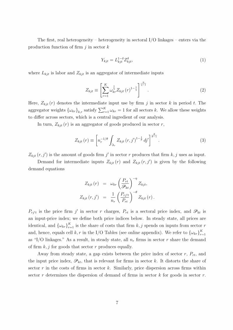
We present these results by focusing on the 10 most and least contractionary sectoral
output contributors to real output effects of monetary shocks. Table 4 reports the
respective cumulative real effects of monetary policy shocks in Panels A and B for our
different cases.
We know from the discussion in section IV that all sectors are equally responsive in
models with homogeneous flexible or sticky prices. The actual response in an economy in
which sectors differ in their degree of price stickiness, sector size, and I/O linkages differs
markedly across sectors. We see in Table A that the 10 least responsive contractionary
sectors have a large and positive response to a contractionary monetary policy shock.
The positive response can happen if these sectors are substantially more flexible than the
average sector in the data which is indeed the case. Sectors with a positive consumption
response have an average frequency of price adjustment that is larger by a factor of 3
relative to the average sector. In panel B, instead, we see very large negative responses
among the 10 most responsive sectors to a contractionary shock.
We see in column (2) and (3) that shutting down either heterogeneity in sector size
or I/O linkages reduces the effective granularity substantially. Both in panel A and B,
we see a large compression in the responses. The most responsive sectors in columns (2)
and (3) respond by only 25% of the response of the most responsive sector in column (1)
with all heterogeneities presents and the range of the responses between sector 1 and 10
shrinks by a factor of 5.
When we shut down both heterogeneity in sector size and I/O linkages and only
focus on differences in price stickiness across sectors, we see an additional compression
to the mean both among the least and most responsive sectors. When we compare the
29

response across columns (1) to (4), we see (i) heterogeneous price stickiness is central for a
differential response across sectors to a common monetary policy shock; (ii) heterogeneity
in sector size and I/O linkages by themselves add to the granularity of the economy
relative to column (4); (iii) it is the inter-linkages between heterogeneity in sector size,
price stickiness, and I/O linkages that have a big effects on the contribution of the most
and least responsive sectors to a common monetary policy shock.
The results in Table 4 show that the intricacies in which different heterogeneities
interact play a crucial role for the relative contribution of different sectors to the aggregate
real effects of monetary policy. Purely focusing on the average impact and cumulative
effects masks substantial heterogeneity across sectoral responses and policy makers that
would aim to stabilize certain sectors would possibly commit policy mistakes by only
focusing on the heterogeneity in price stickiness across sections which is a classical result
in the literature (see Aoki (2001)).
Figure 3 graphically illustrates the identity effects across all 341 sectors when we go
from case 1 in which all heterogeneities are present to case 4 with only heterogeneous
price stickiness across sectors. Rankings change substantially across sectors with some
sectors changing up to 300 ranks. Hence, the exact choice of heterogeneities is clearly
important for the identity of sectors in the transmission mechanism.
Heterogeneity in markups reflects the heterogeneity in real output effects. Price
markups are of independent importance and interest, because they measure the
inefficiency in the economy and are equivalent to a countercyclical labor wedge (see Gali
et al. (2007)). In our setting, the product market wedge is the sole driver of the labor
wedge which is consistent with recent empirical work by Bils, Klenow, and Malin (2014).8
The level of markups in the full model is higher than in the homogeneous benchmark
case, and markups display a rich, dynamic pattern. We report these findings in Figure
A.4 of the online appendix.
The effect of fully interacted heterogeneities in our model becomes clear in comparison
to the completely homogeneous economy. The markup responses of the homogeneous
economy are summarized in Panel (a) of Figure A.4. All sectoral responses are fast-
decaying and identical across all percentiles. The markup response is more than 4.5% on
impact, with a half-life of eight periods.
By contrast, two differential facts emerge for the full model (case 1): First, the median
sectoral response is substantially larger. The initial median markup response increases
to approximately 6%. The dashed, thick blue line summarizes the median response. The
8Shimer (2009) stresses the lack of work on heterogeneity in the product market, a channel we areputting forward and expanding upon by allowing for interactions of different heterogeneities.
30

half-life of the median response is twice as long as in the homogeneous case.
Second, substantial dispersion exists in the markup response. The top 5th percentile
of markups increases to over 10%; the bottom 5th percentile does not increase above 4%.
The sectoral markups also show very different dynamic patterns: The top percentiles
show a hump-shaped response that is very persistent, with a half-life of more than 15
periods. At the same time, the lowest percentiles decay exponentially with a half-life of
less than ten periods. These very different price-markup responses directly result from
the convolutions of the different underlying heterogeneities. They open up new avenues
to study how interactions of different heterogeneities shape inefficiencies in the economy.
C. Sectoral Aggregation and Real Effects
In this section, we study the response of our model economy to monetary policy shocks for
different levels of disaggregation keeping constant the average degree of price stickiness
across levels of aggregation. The choice of aggregation results in large differences in real
effects across model economies. We arrive at this conclusion in two steps.
First, we compare the two levels of granularity published by the BEA: detail
(effectively 341 sectors), summary (56 sectors), and an even coarser aggregation with
only 7 sectors. The left panel of Figure 4 and Table 5 report our findings. Cumulative
real effects of monetary policy are 6% larger in the more disaggregated 341-sector economy
than in the 56-sector calibration but almost 50% larger than in an economy with only
7 sectors which has been the approximate number of sectors in many calibrations in the
literature.
The inflation response is interesting: Upon impact, the inflation response is very
similar across different levels of disaggregation, whereas already large differences exists in
the consumption response across calibrations. Moreover, the inflation response of the 56
sector economy is larger on impact than the response for the 7 sector economy but the
consumption response on impact is also larger for the more disaggregated model. This
finding cautions against drawing inference for monetary policy from the impact response
of inflation to monetary policy shocks.
Second, motivated by these findings as well as our theoretical results in section IV
– that the degree of granularity can matter for the real effects of monetary policy – we
now systematically show the importance of granularity when we aggregate sectors by size
instead of following the BEA aggregation.
In many models, sector size is a good proxy for sector technology. The right panel
of Figure 4 and Table A.2 in the online appendix show the results. The real effects
31

of monetary policy are now dramatically affected. They are more than 40% larger on
impact for the most disaggregated economy compared to the less disaggregated economy
with only 56 sectors, even though the impact response of inflation is again similar. Real
effects are monotonically increasing in the granularity of the economy. Figure A.2 in the
online appendix shows the dispersion in the frequency of price adjustment shrinks for less
granular economies.
What mechanisms are driving these aggregation effects? We find the interactions of
heterogeneities are more important than the convexification of price rigidities in creating
aggregation effects, but they act with some delay. We show the relative importance by
computing the total consumption price paths in a 341 and an 7 sector economy, as well as
the two components from equation (47), due to convexification and interactions. Figure
A.3 in the online appendix illustrates how the two channels contribute to the total gap.
VII Concluding Remarks
We present new theoretical and quantitative insights into the transmission of monetary
policy shocks when heterogeneity in price stickiness, the I/O structure, and sector size
interact.
Although rich theoretical predictions exist for how the interaction of these
heterogeneities shapes the real output effects of monetary shocks, we find in our calibration
to the US economy that heterogeneity in price stickiness is the central mechanism for
generating large and persistent real output effects. Heterogeneity in I/O linkages, instead,
only plays a marginal role. In addition, we document that small-scale models might
substantially underestimate output effects – even though the impact response of inflation
is almost identical across different levels of granularity. We also find that heterogeneity in
price rigidity is key in determining which sectors are the most important contributors to
the transmission of monetary shocks. Finally, while heterogeneity in sector size and I/O
linkages only play a minor role in shaping the aggregate real output effects of monetary
shocks, we find that they jointly increase the effective granularity in the economy.
Our results have important policy implications. First, the impact response of inflation
to a monetary policy shock is not sufficient for the real effects of monetary shocks. Second,
the real effects of more granular economies are substantially larger compared to economies
with only a small number of sectors. And finally, all heterogeneities we study are
important for the identity and contribution of the most important sectors to the real effects
of monetary policy. In particular, sectoral price stickiness is not the only determinant for
the contribution to aggregate real effects. Despite mattering only marginally for the overall
32

real effects, heterogeneity in sector size and I/O linkages are important contributors and
generate an increase in the effective granularity: the most important sectors contributing
to aggregate real effects become even more important, whereas the least important sectors
become even less important. The latter result suggest that central bank should no longer
only focus on stabilizing the prices of the most sticky-price sectors but should jointly focus
on the interaction of sector size, I/O linkages, and price stickiness.
While we study a rich set of heterogeneities at the sectoral level that are we can
directly map into data, we leave out other important differences such as the degree of
durability, differences in intermediate input shares, or heterogeneity in the elasticities
of demand. We hypothesize that more downstream sectors with stickier prices might
also produce more durable goods compared to commodities sectors with flexible prices
and higher elasticities of demand which would possibly amplify real output effects of
monetary shocks. We believe these heterogeneities are important to study but leave a
detailed analysis to future research.
References
Acemoglu, D., U. Akcigit, and W. Kerr (2015). Networks and the macroeconomy: Anempirical exploration. In preparation for: NBER Macroannual .
Acemoglu, D., V. M. Carvalho, A. Ozdaglar, and A. Tahbaz-Salehi (2012). The networkorigins of aggregate fluctuations. Econometrica 80 (5), 1977–2016.
Alvarez, F. E., F. Lippi, and L. Paciello (2016). Monetary shocks in models withinattentive producers. The Review of Economic Studies 83 (2), 421–459.
Aoki, K. (2001). Optimal monetary policy responses to relative-price changes. Journal ofmonetary economics 48 (1), 55–80.
Barrot, J.-N. and J. Sauvagnat (2016). Input specificity and the propagation ofidiosyncratic shocks in production networks. The Quarterly Journal of Economics ,qjw018.
Basu, S. (1995). Intermediate goods and business cycles: Implications for productivityand welfare. The American Economic Review 85 (3), 512–531.
Bhattarai, S. and R. Schoenle (2014). Multiproduct firms and price-setting: Theory andevidence from u.s. producer prices. Journal of Monetary Economics 66, 178–192.
Bigio, S. and J. Lao (2017). Financial frictions in production networks. UnpublishedManuscript, Columbia University .
Bils, M., P. J. Klenow, and B. A. Malin (2014). Resurrecting the role of the productmarket wedge in recessions. Technical report, National Bureau of Economic Research.
Boivin, J., M. P. Giannoni, and I. Mihov (2009). Sticky prices and monetary policy:Evidence from disaggregated U.S. data. The American Economic Review 99 (1), 350–384.
Bouakez, H., E. Cardia, and F. Ruge-Murcia (2014). Sectoral price rigidity and aggregate
33

dynamics. European Economic Review 65, 1–22.
Calvo, G. A. (1983). Staggered prices in a utility-maximizing framework. Journal ofMonetary Economics 12 (3), 383–398.
Carvalho, C. (2006). Heterogeneity in price stickiness and the real effects of monetaryshocks. The B.E. Journal of Macroeconomics 2 (1), 1–56.
Carvalho, C. and J. W. Lee (2011). Sectoral price facts in a sticky-price model.Unpublished Manuscript, PUC-Rio.
Carvalho, C. and F. Schwartzman (2015). Selection and monetary non-neutrality intime-dependent pricing models. Journal of Monetary Economics 76, 141 – 156.
Carvalho, V. M. (2014). From micro to macro via production networks. The Journal ofEconomic Perspectives 28 (4), 23–47.
Coibion, O. and Y. Gorodnichenko (2012). Why are target interest rate changes sopersistent? American Economic Journal: Macroeconomics 4 (4), 126–162.
D’Acunto, F., R. Liu, C. Pflueger, and M. Weber (2016). Flexible prices and leverage.Unpublished manuscript, University of Chicago.
Gabaix, X. (2011). The granular origins of aggregate fluctuations. Econometrica 79 (3),733–772.
Gali, J., M. Gertler, and J. D. Lopez-Salido (2007). Markups, gaps, and the welfare costsof business fluctuations. The review of economics and statistics 89 (1), 44–59.
Gilchrist, S., R. Schoenle, J. Sim, and E. Zakrajsek (2015). Inflation dynamics during thefinancial crisis. Unpublished Manuscript, Brandeis University .
Goldberg, P. P. and R. Hellerstein (2011). How rigid are producer prices? FRB of NewYork Staff Report , 1–55.
Gorodnichenko, Y. and M. Weber (2016). Are sticky prices costly? Evidence from thestock market. American Economic Review 106 (1), 165–199.
Herskovic, B. (2018). Networks in production: Asset pricing implications. The Journalof Finance 73 (4), 1785–1818.
Herskovic, B., B. T. Kelly, H. Lustig, and S. Van Nieuwerburgh (2016). The commonfactor in idiosyncratic volatility: Quantitative asset pricing implications. Journal ofFinancial Economics 119 (2), 249–283.
Huang, K. X. and Z. Liu (2001). Production chains and general equilibrium aggregatedynamics. Journal of Monetary Economics 48 (2), 437 – 462.
Huang, K. X. and Z. Liu (2004). Input–output structure and nominal rigidity: thepersistence problem revisited. Macroeconomic Dynamics 8 (2), 188–206.
Kelly, B., H. Lustig, and S. Van Nieuwerburgh (2013). Firm volatility in granularnetworks. Technical report, National Bureau of Economic Research.
Lucas, R. E. (1977). Understanding business cycles. In Carnegie-Rochester conferenceseries on public policy, Volume 5, pp. 7–29. Elsevier.
Nakamura, E. and J. Steinsson (2008). Five facts about prices: A reevaluation of menucost models. Quarterly Journal of Economics 123 (4), 1415–1464.
Nakamura, E. and J. Steinsson (2010). Monetary non-neutrality in a multi-sector menucost model. Quarterly Journal of Economics 125 (3), 961–1013.
Ozdagli, A. and M. Weber (2017). Monetary policy through production networks:
34

Evidence from the stock market. Unpublished Manuscript, University of Chicago.
Pasten, E., R. Schoenle, and M. Weber (2018). Price rigidity and the origins of aggregatefluctuations. Unpublished manuscript, University of Chicago.
Rudebusch, G. D. (2002). Term structure evidence on interest rate smoothing andmonetary policy inertia. Journal of Monetary Economics 49 (6), 1161–1187.
Shamloo, M. (2010). Price setting in a model with production chains: Evidence fromsectoral data. IMF Working Papers , 1–50.
Shimer, R. (2009). Convergence in macroeconomics: The labor wedge. AmericanEconomic Journal: Macroeconomics 1 (1), 280–297.
Weber, M. (2015). Nominal rigidities and asset pricing. Unpublished manuscript,University of Chicago Booth School of Business .
35

Figure 1: Response of Real Consumption, Inflation, and Real Marginal Coststo Monetary Policy Shock
0 5 10 15 20 25 30-6
-5
-4
-3
-2
-1
0
0 5 10 15 20 25 30-1.5
-1
-0.5
0
0 5 10 15 20 25 30-10
-8
-6
-4
-2
0
case1case2case3case4case5
This figure plots the impulse response function of real consumption, inflation, and real marginal costs to a
one-standard-deviation monetary policy shock for a 341-sector model for different cases (see Table 2 for a
description of the different cases).
36

Figure 2: Response of Real Consumption, Inflation, and Real Marginal Coststo Monetary Policy Shock: Interest-rate Smoothing
0 5 10 15 20 25 30-20
-15
-10
-5
0
0 5 10 15 20 25 30-7
-6
-5
-4
-3
-2
-1
0
=1.24 c=0.33/12
=1.24 c=0.33/12 gc=1.5 i=0.1
=1.24 c=0.33/12 gc=1.5 i=0.5
=1.24 c=0.33/12 gc=1.5 i=0.9
0 5 10 15 20 25 30-25
-20
-15
-10
-5
0
This figure plots the impulse response function of real consumption, inflation, and real marginal costs to a
one-standard-deviation monetary policy shock for a 341-sector model for different cases (see Table 2 for a
description of the different cases) for different Taylor rules with interest-rate smoothing.
37

Figure 3: Ranking of Sectors, Cases 1 and 4
0 50 100 150 200 250 300 3500
50
100
150
200
250
300
350
This figure plots the sectoral rankings for the cumulative IRF for case 1 against case 4 (see Table 2 for a
description of the different cases).
38

Figure 4: Response of Real Consumption and Inflation: Aggregation
Industry-Code Aggregation Size Aggregation
0 5 10 15 20 25 30-6
-5
-4
-3
-2
-1
0
n=341n=56n=7
0 5 10 15 20 25 30-6
-5
-4
-3
-2
-1
0
n=341n=56n=7
0 5 10 15 20 25 30-1.8
-1.6
-1.4
-1.2
-1
-0.8
-0.6
-0.4
-0.2
0
n=341n=56n=7
0 5 10 15 20 25 30-2
-1.8
-1.6
-1.4
-1.2
-1
-0.8
-0.6
-0.4
-0.2
0
n=341n=56n=7
This figure plots the impulse response function of real consumption and inflation to a one-standard-deviation
monetary policy shock for different levels of aggregation. In the left panel, we aggregate sectors by industry
codes and in the right panels, we aggregate based on the sector size always keeping the average frequency of
price adjustment constant.
39

Table 1: Calibration Parameters
This table reports the parameter values of the calibration of the model developed in section IV.
β 0.9975 Monthly discount factor
σ 1 Relative risk aversion
ϕ 2 Inverse of Frisch elasticity
δ 0.5 Average inputs share in production function
η 2 Elasticity of substitution across sectors
θ 6 Elasticity of substitution within sectors
φπ 1.24 Responsiveness of monetary policy to consumption inflation
φc 0.33/12 Responsiveness of monetary policy to output variations
ρ 0.9 Persistence of monetary policy shock
Table 2: Overview of Calibration Cases
This table details the assumptions on frequencies, consumption weights, and input-output linkages for the different
cases employed in the calibration.
Frequencies Consumption Weights Input-Output Linkages
Case 1 sticky, heterogeneous heterogeneous heterogeneous
Case 2 sticky, heterogeneous heterogeneous homogeneous
Case 3 sticky, heterogeneous homogeneous heterogeneous
Case 4 sticky, heterogeneous homogeneous homogeneous
Case 5 sticky, homogeneous homogeneous homogeneous
Table 3: Response to Monetary Policy Shock
This table reports the impact response, the cumulative impulse response, and the persistence of the response
defined as AR(1) coefficient due to a one-percent monetary policy shock for consumption (Panel A), inflation
(Panel B), and real marginal costs (Panel C) for a 350-sector economy for different cases (see Table 2 for a
description of the different cases).
Case 1 Case 2 Case 3 Case 4 Case 5
Panel A. Consumption
Impact −5.09 −5.61 −5.43 −5.72 −3.88
Cumulative IRF −60.40 −61.11 −60.49 −63.42 −37.19
Persistence 0.92 0.90 0.93 0.90 0.87
Panel B. Inflation
Impact −1.46 −1.08 −1.20 −1.10 −1.48
Cumulative IRF −7.10 −6.40 −6.72 −5.60 −14.22
Persistence 0.88 0.88 0.89 0.87 0.87
Panel C. Real Marginal Costs
Impact −6.10 −8.25 −5.99 −6.68 −4.53
Cumulative IRF −82.09 −90.32 −80.44 −73.99 −43.39
Persistence 0.92 0.89 0.91 0.89 0.87
40
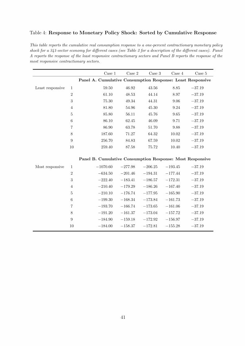
Table 4: Response to Monetary Policy Shock: Sorted by Cumulative Response
This table reports the cumulative real consumption response to a one-percent contractionary monetary policy
shock for a 341-sector economy for different cases (see Table 2 for a description of the different cases). Panel
A reports the response of the least responsive contractionary sectors and Panel B reports the response of the
most responsive contractionary sectors.
Case 1 Case 2 Case 3 Case 4 Case 5
Panel A. Cumulative Consumption Response: Least Responsive
Least responsive 1 59.50 46.92 43.56 8.85 −37.19
2 61.10 48.53 44.14 8.97 −37.19
3 75.30 49.34 44.31 9.06 −37.19
4 81.80 54.96 45.30 9.24 −37.19
5 85.80 56.11 45.76 9.65 −37.19
6 86.10 62.45 46.09 9.71 −37.19
7 86.90 63.78 51.70 9.88 −37.19
8 187.60 71.27 64.32 10.02 −37.19
9 256.70 84.83 67.59 10.02 −37.19
10 259.40 87.58 75.72 10.40 −37.19
Panel B. Cumulative Consumption Response: Most Responsive
Most responsive 1 −1070.60 −277.98 −206.25 −193.45 −37.19
2 −634.50 −201.46 −194.31 −177.44 −37.19
3 −222.40 −183.41 −186.57 −172.31 −37.19
4 −210.40 −179.29 −186.26 −167.40 −37.19
5 −210.10 −176.74 −177.95 −165.90 −37.19
6 −199.30 −168.34 −173.84 −161.73 −37.19
7 −193.70 −166.74 −173.65 −161.06 −37.19
8 −191.20 −161.37 −173.04 −157.72 −37.19
9 −184.90 −159.18 −172.92 −156.97 −37.19
10 −184.00 −158.37 −172.81 −155.28 −37.19
41

Table 5: Response to Monetary Policy Shock (341 vs 56 vs 7 sector economy)
This table reports the impact response, the cumulative impulse response, and the persistence of the response
defined as AR(1) coefficient due to a one-percent monetary policy shock for consumption (Panel A), inflation
(Panel B), and real marginal costs (Panel C) for a 341-sector economy, a 56-sector economy and a 7-sector
economy for case 1 (see Table 2 for a description of the different cases).
341 Sectors 56 Sectors 7 Sectors
Panel A. Consumption
Impact −5.09 −4.71 −3.89
Cumulative IRF −60.40 −56.79 −40.56
Persistence 0.92 0.90 0.94
Panel B. Inflation
Impact −1.46 −1.62 −1.56
Cumulative IRF −7.10 −8.34 −13.65
Persistence 0.88 0.88 0.90
Panel C. Real Marginal Costs
Impact −6.10 −4.21 −4.82
Cumulative IRF −82.09 −53.94 −58.02
Persistence 0.92 0.90 0.88
42

Online Appendix:Production Networks and the Propagation of
Monetary Policy ShocksErnesto Pasten, Raphael Schoenle, and Michael Weber
Not for Publication
I Log-linearized System
A. Steady-State Solution
The steady state equilibrium sets the same prices for all firms
PC = Pk = Pk = P (A.1)
such that
Ck = ωckC,
Cjk =1
nkCk,
Zjk (k′) = ωkk′Z,
Zjk (j′, k′) =1
nk′Zjk (k′) .
All firms produce the quantity, so Yjk = Y , and
Yjk = Cjk +K∑k′=1
∫=k′
Zj′k′ (j, k) dj′,
Ykt = Ckt +K∑k′=1
Zk′ (k) ,
Yt = Ct + Zt
given that the labor and intermediate inputs share are the same for all firms in steady
1

state,
Yjk = Y ;
Ljk = L;
Zjk = Z.
By aggregation, it holds that
C =K∑k=1
∫=kCjkdj,
Z =K∑k′=1
∫=k′
Zjk (j′, k′) dj′.
so,
Y = C + Z,
nk = (1− ψ)ωck +K∑k′=1
nk′ωk′k.
In turn, steady-state labor supply from equation is
Wk
P= gkL
ϕkC
σ. (A.2)
In a symmetric steady state, Lk = nkL, so this steady state exists if gk = n−ϕk such
that Wk = W for all k. Thus, steady-state labor supply is given by
W
P= LϕCσ. (A.3)
Households’ budget constraint, firms’ profits, production function, efficiency of
2
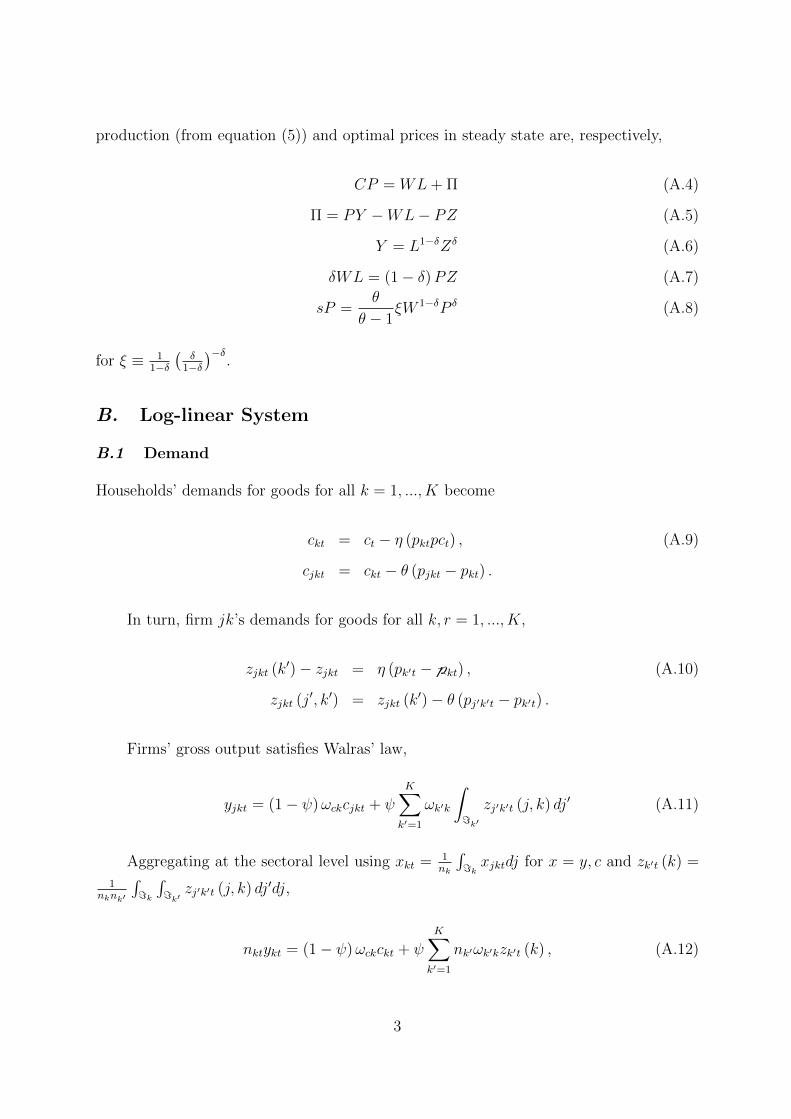
production (from equation (5)) and optimal prices in steady state are, respectively,
CP = WL+ Π (A.4)
Π = PY −WL− PZ (A.5)
Y = L1−δZδ (A.6)
δWL = (1− δ)PZ (A.7)
sP =θ
θ − 1ξW 1−δP δ (A.8)
for ξ ≡ 11−δ
(δ
1−δ
)−δ.
B. Log-linear System
B.1 Demand
Households’ demands for goods for all k = 1, ..., K become
ckt = ct − η (pktpct) , (A.9)
cjkt = ckt − θ (pjkt − pkt) .
In turn, firm jk’s demands for goods for all k, r = 1, ..., K,
zjkt (k′)− zjkt = η (pk′t −pkt) , (A.10)
zjkt (j′, k′) = zjkt (k′)− θ (pj′k′t − pk′t) .
Firms’ gross output satisfies Walras’ law,
yjkt = (1− ψ)ωckcjkt + ψK∑k′=1
ωk′k
∫=k′
zj′k′t (j, k) dj′ (A.11)
Aggregating at the sectoral level using xkt = 1nk
∫=kxjktdj for x = y, c and zk′t (k) =
1nknk′
∫=k
∫=k′
zj′k′t (j, k) dj′dj,
nktykt = (1− ψ)ωckckt + ψK∑k′=1
nk′ωk′kzk′t (k) , (A.12)
3

and, at the aggregate level using yt =∑
k nkykt, ct =∑
k ωckckt and zt =∑Kk=1
∑Kk′=1 ωk′knk′zk′t (k) ,
yt = (1− ψ) ct + ψzt. (A.13)
B.2 IS and Labor Supply
The household Euler equation becomes
ct = Et [ct+1]− σ−1 it − (Et [pct+1]− pt) . (A.14)
The labor supply condition is
wkt − pct = ϕlkt + σct. (A.15)
B.3 Firms
Production function:
yjkt = akt + (1− δ) ljkt + δzjkt. (A.16)
Efficiency condition:
wkt −pkt = zjkt − ljkt. (A.17)
Marginal costs:
mckt = (1− δ)wkt + δpkt − akt. (A.18)
Optimal reset price:
p∗kt = (1− αkβ)mckt + αkβEt[p∗kt+1
]. (A.19)
Sectoral prices:
pkt = (1− αk) p∗kt + αkpkt−1. (A.20)
The monetary policy rule must be added to close the model. In the main text
sometimes we use money supply assuming
ct + pct = mt (A.21)
4

and, when specified, we use a Taylor rule,
it = φπ (pct − pct−1) + φcct. (A.22)
II Proofs
Proposition 1
Proof. When αk = α for all k, we aggregate equations (43) using consumption weights
to obtain
pct (α) =(1− δ) (1− α)
1− δ (1− α)mt +
α
1− δ (1− α)pct−1 (α) .
Equation (45) follows by using the previous expression to solve for pct (α) when a
permanent monetary shock m hits at t∗. (1) and (2) follow directly from equation (45).
Proposition 2
Proof. The restriction ωkk′ = ωck′ for all k, k′ implies pkt = pct for all k. Thus, according
to equation (43), sectoral prices solve
pkt = (1− αk) [(1− δ)mt + δpct] + αkpkt−1.
Iterating backwards and using pct =∑K
k=1 ωckpkt yields equation (46).
(1) follows from setting pkt = 0 for t < t∗ and for t = t∗, (∑
k ωckαk − α) = 0.
For (2), denote pct (α) the solution for aggregate consumption prices in Proposition
1. Further assume pct−s = pct−s (α). Hence,
pct − pct (α) = − (1− δ)m1− δ (1− α)
(K∑k=1
ωckαt−t∗+1k − αt−t∗+1
)
+δ
1− δ (1− α)
t−t∗∑τ=1
(K∑k=1
ωckατk (1− αk)− ατ (1− α)
)pct−τ .
Jensen’s inequality, pct − pct (α) ≤ 0 and decreases in the dispersion of price stickiness
across sectors, αkkk=1. In addition, pct−s ≤ pct−s for all s ≥ 1, which reinforces the
result.
5

Proposition 3
Proof. Let pct denote the response of aggregate consumption prices in Proposition 2.
Assume pkt−s = pkt−s for all s ≥ 1. Subtracting equation (46) from equation (47) yields
pct − pct = δ
K∑k=1
(ukpkt − (1− α)ωckpkt) + δ
t−t∗∑τ=1
(K∑k′=1
ωck′ατk′ (1− αk′)
)K∑k=1
(ωk − ωck) pkt−τ
+δKt−t∗∑τ=1
K∑k=1
COV (ωck′ατk′ (1− αk′) , ωk′k) pkt−τ ,
(A.23)
for uk ≡∑K
k′=1 ωck′ (1− αk′)ωk′k and ωk ≡ 1K
∑Kk′=1 ωk′k.
For (1), we use pkt = 0 for t < t∗, so pct < pct whenK∑k=1
(ukpkt − (1− α)ωckpkt) < 0.
This inequality holds when for the sectors with most sticky prices uk > (1− α)ωck.
For (2), two additional terms come to play. The second term of equation (A.23)
is negative when for the sectors with most sticky prices ωk > ωck. The third term of
equation (A.23) is negative when the covariance term is positive for the most sticky sectors
and negative for the most flexible sectors. Relaxing the assumption that pkt−s = pkt−s
reinforces these results.
Finally, we can derive an expression that only contains parameters and the monetary
policy shock on the right-hand side. We have that
pkt = (1− δ) (1− αk)m+ δ (1− αk)pkt + αkpkt−1 (A.24)
which in matrix form using the sectoral price vector pt becomes
pt = [I− δ (I− A) Ω]−1 [(1− δ) (I− A) ιm+ Apt−1] (A.25)
where ι is a vector of ones and A is a diagonal matrix of αk. Solving backwards yields
ekΩC (1− δ)
[I− [I− δ (I− A) Ω]−1 (I− A)
]−1[I−([I− δ (I− A) Ω]−1 (I− A)
)t−t∗+1]
[I− δ (I− A) Ω]−1 (I− A) ιm.
(A.26)
Proposition 4
6

Proof. When δ = 0,
pkt = (1− αk)mt + αkpkt−1 for all k (A.27)
such that
pct =
(1−
K∑k=1
ωckαt−t∗+1k
)m,
pct =
1−K/2∑k′=1
ωck′αt−t∗+1k′
m
Thus,
pct − pct =
K/2∑k′=1
ωck′[λk′α
t−t∗+12k′−1 + (1− λk′)αt−t
∗+12k′ − αt−t∗+1
k′
](A.28)
for any period t ≥ t∗.
It follows from Jensen’s inequality
λk′αt−t∗+12k′−1 + (1− λk′)αt−t
∗+12k′ − αt−t∗+1
k′ > 0 (A.29)
for α2k′−1 6= α2k′ and t > t∗. The previous expression decreases in |α2k′−1 − α2k′ | and
reaches its minimum for
λ∗ (t) =
[1
t−t∗+1
(αt−t
∗+12k′−1 − α
t−t∗+12k′
)] 1t−t∗
(α2k′−1 − α2k′)t−t∗+1t−t∗
− α2k′
α2k′−1 − α2k′, (A.30)
given α2k′−1 and α2k′ .
Proposition 5
Proof. Sectoral prices now solve
pkt = (1− αk) [(1− δ)mt + δpct] + αkpkt−1 for all k (A.31)
7

such that
pct =1− δ
1− δ (1− α)
(1−
K∑k=1
ωckαt−t∗+1k
)m+
δ
1− δ (1− α)
t−t∗∑τ=1
(K∑k=1
ωckατk (1− αk)
)pct−τ ,
pct =1− δ
1− δ (1− α)
1−K/2∑k′=1
ωck′αt−t∗+1k′
m+δ
1− δ (1− α)
t−t∗∑τ=1
K/2∑k′=1
ωck′ατk (1− αk)
pct−τ .
for any period t ≥ t∗.
Assume that pct−τ = pct−τ for all τ ≥ 1, so
pct − pct = − 1− δ1− δ (1− α)
K/2∑k′=1
ωck′(λk′α
t−t∗+12k′−1 + (1− λk′)αt−t
∗+12k′ − αt−t
∗+1k′
)m
+δ
1− δ (1− α)
t−t∗∑τ=1
K/2∑k′=1
ωck′
λk′ (1− α2k′−1)ατ2k′−1 + (1− λk′) (1− α2k′)ατ2k′
− (1− αk′)ατk′
pct−τ(A.32)
The difference pct− pct is a sum of two terms. The first term in equation (A.32) is a
rescaled analogue of the preceeding price stickiness convexification so results (i)–(iv) still
apply. The second term is a measure of the amplification of monetary non-neutrality due
to strategic complementary introduced by intermediate inputs. The higher this term, the
smaller is pct relative to pct.
From Jensen’s inequality
λk′ (1− α2k′−1)ατ2k′−1 + (1− λk′) (1− α2k′)ατ2k′ − (1− αk′)ατk′ < 0 (A.33)
for α2k′−1 6= α2k′ and t > t∗.
Thus, the difference in the consumption price response between baseline and merged
economies, pct − pct, is larger when the difference in frequencies, α, is higher for merged
sectors with higher combined weight, ωck′ . Relaxing the assumption pct−τ = pct−τ for all
τ ≥ 1 reinforces the result regarding frequencies.
Proposition 6
Proof. This proposition follows entirely analogously to the preceeding ones, allowing for
unrestricted heterogeneity in I/O linkages and given the pricing expression in Proposition
3.
8

III Industry by Industry Input-Output Matrix
We use the make table (MAKE) to determine the share of each commodity c that each
industry i produces. We define the market share (“SHARE”) of industry i’s production
of commodity c as
SHARE = MAKE (I×MAKE)−1i,j , (A.34)
where I is a matrix of 1s with suitable dimensions.
We multiply the share and use tables (USE) to calculate the dollar amount that
industry i sells to industry j. We label this matrix revenue share (REV SHARE), which
is a supplier industry-by-consumer industry matrix,
REV SHARE = (SHARE × USE). (A.35)
We use the revenue share matrix to calculate the percentage of industry j’s inputs
purchased from industry i and label the resulting matrix SUPPSHARE:
SUPPSHARE = REV SHARE ((USE × I)−1i,j )>. (A.36)
The input-share matrix in equation (A.36) is an industry-by-industry matrix and therefore
consistently maps into our model.
IV Robustness
In this subsection, we first show how the specification of monetary policy affects our
conclusions. We then analyze how changes in parameters and tails of the frequency
distribution affect our findings.
As the first set of robustness checks, we vary the parameters of the Taylor rule. We
also study a specification with exogenous nominal demand, rather than closing the model
with a Taylor rule. We report the results in Figure A.5 and Table A.3 for the same five
cases.
As our first experiment, we increase φπ, the systematic response of monetary policy
to inflation in the Taylor rule, from a baseline value of 1.24 to 2.5.
9

We see in Figure A.5 a similar response of inflation independent of whether we study
heterogeneous or homogeneous price stickiness, sector size, and I/O structure. The impact
response of inflation is, however, roughly cut to one-third compared to our baseline in
Figure 1, which comes from weaker demand effects. The inflation response tends to be
slightly more persistent with all three forms of heterogeneity, but the cumulative inflation
responses in an economy with φπ = 2.5 are still smaller than in an economy with φπ = 1.24
(compare panels B of Table 3 and Table A.3).
The higher systematic response to inflation in the Taylor rule reduces the impact
response of consumption by a factor of up to four across different cases (compare panels A
of Table 3 and Table A.3). A model with heterogeneous price stickiness but homogeneous
sector size and I/O structure has an almost twice as large impact response compared to
an economy in which all three forms of heterogeneities interact (case 3 vs. case 1). A
higher weight on inflation stabilization in the Taylor rule for a given demand shock results
in a larger stabilization of output in the standard New Keynesian model. Once we allow
for heterogeneous price stickiness, the cumulative real effects of monetary policy shocks
contract by 40%, with a more stringent response to inflationary pressure in the Taylor rule.
We see similar results once we add heterogeneity in sector size and I/O structure. We see
in Panels A and C of Table 3 and Table A.3 that the different forms of heterogeneity
introduce a slightly more sluggish and persistent response in consumption and real
marginal costs, which explains the large real effects of demand shocks, despite the smaller
effects on impact. This finding is reminiscent of the responder-nonresponder framework
discussed in Carvalho (2006) and the selection effect of Carvalho and Schwartzman (2015).
Changes in the systematic response to output growth have little impact on the
response of real consumption, inflation, or real marginal costs (not tabulated).
In our second experiment, we close the model by positing exogenous nominal demand.
Figure A.6 reports our findings. The dashed blue line represents our baseline response
with the Taylor rule, and the dash-dotted blue line represents the response for a model
with exogenous nominal demand. Real marginal costs barely move in the model with
exogenous demand, resulting in a small and transient impact response of inflation and
a one-percentage-point response of consumption on impact. The impact response of
consumption is smaller by a factor of five than the impact response with a Taylor rule.
As a second set of robustness checks, we analyze how changes in parameters and tails
10

of the frequency distribution affect our findings. First, we study the effect of changes in
risk aversion, σ, the Frisch elasticity, ϕ, the average input share in production, δ, the
elasticity of substitution within and across sectors, η, θ, and the persistence of monetary
policy shocks, ρ, in our full-blown model (case 1 in Table 2). Specifically, we set (baseline
parameters in parentheses) σ = 2(1), ϕ = 1(2), δ = 0.7(0.5), η = 6(2), θ = 10(6), and
ρ = 0.95(0.90). Figure A.7 and Table A.4 report our findings.
Overall, we see our results in the baseline calibration of Table 3 and Figure 1 are
robust to variations in parameter values. The only exception is the increase of the
coefficient of relative risk aversion, σ, from a baseline value of 1 to 2. The intratemporal
rate of substitution from leisure to consumption determines the real wage. The drop in
consumption results in a drop in the real wage, which increases in σ. Lower real wages
lower the response of real marginal costs and the overall demand pressure.
V Proofs
In our first case, the full set of heterogeneities is present and firms in different sectors
differ by their degree of price stickiness and intermediate input usage and sectors differ in
size. We see in Table 3 and Figure 1 large real effect of monetary policy on impact that
are persistent over time. Real effects are large compared to a New Keynesian model with
fully flexible prices in which prices fully absorb the monetary policy shock, and we do not
see any effect on real consumption or marginal costs.
Case 2 is similar to case 1 but imposes intermediate input shares that are
homogeneous and equal across sectors. This case corresponds to Proposition 3 in
the simplified model, where we allow consumption and I/O weights to differ. In the
calibration, we find imposing homogeneous I/O linkages results in real effects both on
impact and in total that are similar to our baseline calibration in which we allow for all
heterogeneities to interact.
In case 3 instead, we impose homogeneous sector size but heterogeneous I/O linkages
and case 4 imposes both homogeneous sector size and I/O linkages. Under the assumptions
of case 4, however, sectoral weights of all aggregate prices are the same, so that pkt =
pct = pt for all sectors k, and the wedges between price indices that affect marginal cost
are absent. We see relative to case 1 only small variations, and real output effects, the
11

inflation response or how marginal costs react are similar across the different cases.
Finally in case 5, we introduce homogeneity in price stickiness and keep sectoral
size and I/O linkages homogeneous. We see in Figure 1 that now real effects drop
substantially and inflation responds more immediately. The reason for the larger real
effects in economies with heterogeneous price stickiness is a negative selection effect –
older prices are less likely to change, and real output effects are larger – an effect that
dominates any of the other factors that influence markups, and real effects of monetary
policy are now substantially larger and the price effect is muted.
In calibrations with heterogeneous price stickiness, we see the real effects of monetary
policy both on impact and cumulatively more than double compared to an economy with
homogeneous but equal average price stickiness (see Table 3). The inflation response,
instead, is substantially muted (see blue dashed line in Figure 1). Our results confirm the
intuition for economies with heterogeneity in price setting of Carvalho and Schwartzman
(2015) and Nakamura and Steinsson (2010) and Proposition 2 in our simplified model.
Relative to the model predictions, the impact difference in the price response relative to
the previous case also highlights the role of forward-looking price setters.
12

Figure A.1: Distribution of the Frequency of Price Adjustment
0 0.1 0.2 0.3 0.4 0.5 0.6 0.7 0.8 0.9 10
20
40
60
80
100
120
140
This figure plots the distribution of the frequency of price adjustment for a 341-sector model using the
microdata underlying the PPI from the BLS.
13

Figure A.2: Variance of Frequency of Price adjustment: Size Aggregation
0 50 100 150 200 250 300 3500
0.005
0.01
0.015
0.02
0.025
0.03
0.035
0.04
0.045
0.05
This figure plots the variance of the frequency of price adjustments for different levels of aggregation. We
aggregate sectors by the sector size keeping the average frequency of price adjustment constant.
14

Figure A.3: Price Gap and Components, 341 and 7 Sectors
0 10 20 30 40 50 60-0.02
0
0.02
0.04
0.06
0.08
0.1
0.12
0.14
0.16
Price stickiness convexification
Heterogeneity interaction
Total Price Gap
This figure plots the the price gap of the 7 less the 341 sector consumption price path, and the difference in
the convexification and interaction components implied by equation (47) that make up the price paths.
15

Figure A.4: Response of Markups to Monetary Policy Shock
0 5 10 15 20 25 300
0.5
1
1.5
2
2.5
3
3.5
4
4.5
5Panel A
5th Percentile10th Percentile25th PercentileMedian75th Percentile90th Percentile95th Percentile
0 5 10 15 20 25 300
2
4
6
8
10
12Panel B
5th Percentile10th Percentile25th PercentileMedian75th Percentile90th Percentile95th Percentile
This figure plots the impulse response function of markups to a one-standard-deviation monetary policy shock
for a 341-sector model for case 5 in Panel A and case 1 in Panel B (see Table 2 for a description of the
different cases).
16

Figure A.5: Response of Real Consumption, Inflation, and Real Marginal Coststo Monetary Policy Shock (φπ = 2.5)
0 5 10 15 20 25 30-3
-2.5
-2
-1.5
-1
-0.5
0
0 5 10 15 20 25 30-0.7
-0.6
-0.5
-0.4
-0.3
-0.2
-0.1
0
0 5 10 15 20 25 30-4
-3
-2
-1
0
case1case2case3case4case5
This figure plots the impulse response function of real consumption, inflation, and real marginal costs to a
one-standard-deviation monetary policy shock for a 341-sector model for different cases (see Table 2 for a
description of the different cases) with a coefficient on inflation in the Taylor rule of φπ = 2.5.
17

Figure A.6: Response of Real Consumption, Inflation, and Real Marginal Coststo Monetary Policy Shock (exogenous nominal demand)
0 5 10 15 20 25 30-6
-5
-4
-3
-2
-1
0
1
0 5 10 15 20 25 30-1.5
-1
-0.5
0
0 5 10 15 20 25 30
-6
-5
-4
-3
-2
-1
0
Endog. Nom. DemandExog. Nom. Demand
This figure plots the impulse response function of real consumption, inflation, and real marginal costs to a
one-standard-deviation monetary policy shock for a 341-sector model for case 1 (see Table 2 for a description
of the different cases), closing the model with positing exogenous nominal demand.
18

Figure A.7: Response of Real Consumption, Inflation, and Real Marginal Coststo Monetary Policy Shock (variations in parameters)
0 5 10 15 20 25 30-7
-6
-5
-4
-3
-2
-1
0
0 5 10 15 20 25 30-3
-2.5
-2
-1.5
-1
-0.5
0
0.5
0 5 10 15 20 25 30-8
-7
-6
-5
-4
-3
-2
-1
0
Base Case=2
=1
=0.7
=6
=10=0.95
This figure plots the impulse response function of real consumption, inflation, and real marginal costs to a
one-standard-deviation monetary policy shock for a 341-sector model for case 1 (see Table 2) for different
values of structural parameters.
19

Table A.1: Descriptive StatisticsThe table reports the moments of the frequency of price adjustment, FPA, distribution for a 7-sector model in
panel A , 56-sector model in panel B and a 341-sector model in panel C using the microdata underlying the PPI
from the BLS.
Mean Median Std 25th Pct 75th Pct
Panel A. 7 Sector Economy
FPA 0.17 0.10 0.17 0.07 0.19
Panel B. 56 Sector Economy
FPA 0.18 0.13 0.19 0.08 0.24
Panel C. 341 Sector Economy
FPA 0.15 0.17 0.22 0.08 0.21
20

Table A.2: Response to Monetary Policy Shock: Size Aggregation (341 vs 56vs 7 sector economy)
This table reports the impact response, the cumulative impulse response, and the persistence of the response
defined as AR(1) coefficient due to a one-percent monetary policy shock for consumption (Panel A), inflation
(Panel B), and real marginal costs (Panel C) for a 341-sector economy, a 56-sector economy and a 7-sector
economy for case 1 (see Table 2 for a description of the different cases). We aggregate sectors by size.
341 Sectors 56 Sectors 7 Sectors
Panel A. Consumption
Impact −5.09 −3.64 −3.60
Cumulative IRF −60.40 −43.21 −33.62
Persistence 0.92 0.93 0.83
Panel B. Inflation
Impact −1.46 −1.90 −1.55
Cumulative IRF −7.10 −12.93 −15.51
Persistence 0.88 0.92 0.85
Panel C. Real Marginal Costs
Impact −6.10 −1.80 −5.69
Cumulative IRF −82.09 −42.28 −50.61
Persistence 0.92 0.94 0.85
21

Table A.3: Response to Monetary Policy Shock (φπ = 2.5)
This table reports the impact response, the cumulative impulse response, and the persistence of the response
defined as AR(1) coefficient due to a one-percent monetary policy shock for consumption (Panel A), inflation
(Panel B), and real marginal costs (Panel C) for a 341-sector economy for different cases (see Table 2 for a
description of the different cases) with a coefficient on inflation in the Taylor rule of φπ = 2.5.
Case 1 Case 2 Case 3 Case 4 Case 5
Panel A. Consumption
Impact −1.83 −2.41 −2.23 −2.58 −1.35
Cumulative IRF −30.92 −32.99 −31.91 −36.92 −12.96
Persistence 0.94 0.92 0.94 0.93 0.87
Panel B. Inflation
Impact −0.67 −0.55 −0.60 −0.60 −0.52
Cumulative IRF −4.31 −3.96 −4.07 −3.76 −4.95
Persistence 0.92 0.91 0.92 0.90 0.87
Panel C. Real Marginal Costs
Impact −2.22 −3.54 −2.49 −3.01 −1.58
Cumulative IRF −42.34 −48.77 −42.80 −43.08 −15.12
Persistence 0.94 0.91 0.94 0.92 0.87
22

Table A.4: Response to Monetary Policy Shock (variations in parameters)
This table reports the impact response, the cumulative impulse response, and the persistence of the response
defined as AR(1) coefficient due to a one-percent monetary policy shock for consumption (Panel A), inflation
(Panel B), and real marginal costs (Panel C) for a 341-sector economy for case 1 (see Table 2) for different
values of structural parameters.
Base σ = 2 φ = 1 δ = 0.7 η = 6 θ = 10 ρ = 0.95
Panel A. Consumption
Impact −5.09 −3.23 −5.59 −6.36 −5.51 −5.03 −5.83
Cumulative IRF −60.40 −36.09 −63.90 −67.14 −60.04 −58.70 −115.22
Persistence 0.92 0.91 0.91 0.91 0.92 0.92 0.94
Panel B. Inflation
Impact −1.46 −1.19 −1.20 −0.74 −1.15 −1.43 −2.52
Cumulative IRF −7.10 −5.52 −5.69 −4.07 −6.57 −7.59 −25.89
Persistence 0.88 0.87 0.88 0.88 0.85 0.89 0.91
Panel C. Real Marginal Costs
Impact −6.10 −5.15 −4.99 −4.10 −7.10 −7.39 −7.04
Cumulative IRF −82.09 −65.32 −63.85 −51.20 −87.61 −97.21 −158.88
Persistence 0.92 0.91 0.91 0.91 0.91 0.91 0.94
23


![Propagation of Shocks due to Natural Disasters through Global …€¦ · Propagation of Shocks due to Natural Disasters through Global Supply Chains* [Preliminary. Do not cite.]](https://img.pdfslide.us/doc/110x75/600b2e9e05bc0301205de602/propagation-of-shocks-due-to-natural-disasters-through-global-propagation-of-shocks.jpg)