Embed Size (px)
Citation preview
The Pennsylvania State University
The Graduate School
WIND ESTIMATION AND CLOSED-LOOP CONTROL OF A SOARING
VEHICLE
A Thesis in
Aerospace Engineering
by
John Bird
c© 2013 John Bird
Submitted in Partial Fulfillment
of the Requirements
for the Degree of
Master of Science
December 2013
The thesis of John Bird was reviewed and approved∗ by the following:
Jacob W. LangelaanAssociate Professor of Aerospace EngineeringThesis Advisor
Mark D. MaughmerProfessor of Aerospace Engineering
George A. LesieutreProfessor of Aerospace EngineeringDepartment Head, Aerospace Engineering
∗Signatures are on file in the Graduate School.
Abstract
Birds possess a remarkable ability to harvest energy from the atmosphere, allowing them totraverse vast regions foraging for food. From the thermalling flights of raptors and vulturesto the astonishing flights of the albatross in the maritime wind shear, birds have shown thattheir soaring ability is diverse and adaptable, making such techniques of interest for improvingperformance of small uninhabited air vehicles.
This thesis investigates techniques to map the wind field surrounding an aircraft and then toexploit that wind field for energy to sustain flight. Wind is accomplished through the use of theKalman filter and its nonlinear variants applied to spline models and selected model functions.Both arbitrary two-dimensional updraft fields and vertical wind shears with anticipated formsare investigated through simulation and some flight experiments.
Exploitation strategies and path following controllers to exploit wind maps are also investi-gated. A contour approach is used to exploit two-dimensional maps of convective updrafts, whilea trajectory planning and selection system is used to exploit vertical shear of the horizontal wind.Path following controllers are developed to guide the aircraft on energy harvesting trajectoriesin both environments, and their suitability is investigated in simulation.
The final result is a system that allows an aircraft with no knowledge of the wind fieldgather information, plan energy harvesting paths, follow the required trajectory, and update thetrajectory as information is gathered. This system closes a loop around the energy harvestingproblem. Batch and hardware in the loop simulation is used to establish the capability of thesystem.
iii
Table of Contents
List of Figures vii
List of Tables ix
Acknowledgments x
Chapter 1Energy Harvesting for Small Uninhabited Aerial Systems 11.1 Intelligent Systems in Resource-Constrained Applications . . . . . . . . . . . . . 11.2 Energy Harvesting . . . . . . . . . . . . . . . . . . . . . . . . . . . . . . . . . . . 2
1.2.1 Static Soaring . . . . . . . . . . . . . . . . . . . . . . . . . . . . . . . . . . 21.2.1.1 Thermal . . . . . . . . . . . . . . . . . . . . . . . . . . . . . . . 31.2.1.2 Wave . . . . . . . . . . . . . . . . . . . . . . . . . . . . . . . . . 31.2.1.3 Ridge or Slope . . . . . . . . . . . . . . . . . . . . . . . . . . . . 4
1.2.2 Dynamic Soaring . . . . . . . . . . . . . . . . . . . . . . . . . . . . . . . . 41.2.3 Gust Soaring . . . . . . . . . . . . . . . . . . . . . . . . . . . . . . . . . . 6
1.3 A Control Architecture for Soaring . . . . . . . . . . . . . . . . . . . . . . . . . . 61.4 Wind Modeling . . . . . . . . . . . . . . . . . . . . . . . . . . . . . . . . . . . . . 61.5 Contributions . . . . . . . . . . . . . . . . . . . . . . . . . . . . . . . . . . . . . . 71.6 Readers Guide . . . . . . . . . . . . . . . . . . . . . . . . . . . . . . . . . . . . . 7
Chapter 2Vehicle and Environment Models 82.1 Mapping, Planning, and Control for Soaring . . . . . . . . . . . . . . . . . . . . . 82.2 Vehicle Model . . . . . . . . . . . . . . . . . . . . . . . . . . . . . . . . . . . . . . 8
2.2.1 Kinematic Thermalling Model . . . . . . . . . . . . . . . . . . . . . . . . 92.2.2 Dynamic Soaring Equations of Motion . . . . . . . . . . . . . . . . . . . . 102.2.3 Six Degree of Freedom Model for HiL Simulation . . . . . . . . . . . . . . 12
2.3 Environmental Models . . . . . . . . . . . . . . . . . . . . . . . . . . . . . . . . . 132.3.1 Thermal Models . . . . . . . . . . . . . . . . . . . . . . . . . . . . . . . . 142.3.2 Ridge Shear Model . . . . . . . . . . . . . . . . . . . . . . . . . . . . . . . 142.3.3 Turbulence Model . . . . . . . . . . . . . . . . . . . . . . . . . . . . . . . 15
2.4 Vehicle-Environment Interactions: Energy Harvesting . . . . . . . . . . . . . . . 16
iv
2.4.1 The DS Rule and Shear . . . . . . . . . . . . . . . . . . . . . . . . . . . . 162.4.2 Direct Computation of Wind Field . . . . . . . . . . . . . . . . . . . . . . 18
Chapter 3Wind Mapping 213.1 Kalman Filters, Estimation, and Wind Mapping . . . . . . . . . . . . . . . . . . 213.2 Mapping an a priori Determined Structure . . . . . . . . . . . . . . . . . . . . . 21
3.2.1 Variability of the Mean Wind Field . . . . . . . . . . . . . . . . . . . . . . 213.2.1.1 Boundary Layer Shear . . . . . . . . . . . . . . . . . . . . . . . . 223.2.1.2 Ridge Shear . . . . . . . . . . . . . . . . . . . . . . . . . . . . . 22
3.2.2 Modeling Wind Profiles With the Kalman Filter . . . . . . . . . . . . . . 233.3 Mapping Arbitrary Wind Structures . . . . . . . . . . . . . . . . . . . . . . . . . 24
3.3.1 Spline Mathematics . . . . . . . . . . . . . . . . . . . . . . . . . . . . . . 243.3.2 Wind Mapping with Splines . . . . . . . . . . . . . . . . . . . . . . . . . . 26
3.4 Combined Model and Model-Free Wind Mapping . . . . . . . . . . . . . . . . . . 273.5 1-D Mapping Results . . . . . . . . . . . . . . . . . . . . . . . . . . . . . . . . . . 28
3.5.1 Simulations . . . . . . . . . . . . . . . . . . . . . . . . . . . . . . . . . . . 283.5.2 Fox Boundary-Layer Data . . . . . . . . . . . . . . . . . . . . . . . . . . . 283.5.3 Ridge Shear Modeling Simulation . . . . . . . . . . . . . . . . . . . . . . . 29
3.6 Mapping Multi-Dimensional Wind Structures . . . . . . . . . . . . . . . . . . . . 303.6.1 Thermal Simulation Results . . . . . . . . . . . . . . . . . . . . . . . . . . 31
Chapter 4Optimizing Thermal Soaring 334.1 Thermal Contour Paths . . . . . . . . . . . . . . . . . . . . . . . . . . . . . . . . 334.2 Closed-loop Control . . . . . . . . . . . . . . . . . . . . . . . . . . . . . . . . . . 344.3 Simulation Results . . . . . . . . . . . . . . . . . . . . . . . . . . . . . . . . . . . 36
4.3.1 Vehicle Model . . . . . . . . . . . . . . . . . . . . . . . . . . . . . . . . . . 374.3.2 Simulation Results . . . . . . . . . . . . . . . . . . . . . . . . . . . . . . . 37
Chapter 5Dynamic Soaring 425.1 Dynamic Soaring at Ridges . . . . . . . . . . . . . . . . . . . . . . . . . . . . . . 425.2 Control Architecture . . . . . . . . . . . . . . . . . . . . . . . . . . . . . . . . . . 42
5.2.1 Global Planner . . . . . . . . . . . . . . . . . . . . . . . . . . . . . . . . . 435.2.2 Local Planner . . . . . . . . . . . . . . . . . . . . . . . . . . . . . . . . . . 445.2.3 Wind Mapper . . . . . . . . . . . . . . . . . . . . . . . . . . . . . . . . . . 445.2.4 Piccolo Communications . . . . . . . . . . . . . . . . . . . . . . . . . . . . 44
5.3 Global Planning . . . . . . . . . . . . . . . . . . . . . . . . . . . . . . . . . . . . 445.4 Closed-loop Control . . . . . . . . . . . . . . . . . . . . . . . . . . . . . . . . . . 455.5 DS Control with the Piccolo Autopilot . . . . . . . . . . . . . . . . . . . . . . . . 475.6 Hardware-in-the-Loop Simulations . . . . . . . . . . . . . . . . . . . . . . . . . . 48
5.6.1 Simulations in Smooth Air . . . . . . . . . . . . . . . . . . . . . . . . . . 495.6.2 Light Turbulence . . . . . . . . . . . . . . . . . . . . . . . . . . . . . . . . 495.6.3 Wind Mapper Performance . . . . . . . . . . . . . . . . . . . . . . . . . . 52
v
Chapter 6Conclusions 546.1 Use of Wind Maps in Energy Harvesting . . . . . . . . . . . . . . . . . . . . . . . 54
6.1.1 Static Soaring . . . . . . . . . . . . . . . . . . . . . . . . . . . . . . . . . . 546.1.2 Dynamic Soaring . . . . . . . . . . . . . . . . . . . . . . . . . . . . . . . . 54
6.2 Recommendations for Future Work . . . . . . . . . . . . . . . . . . . . . . . . . . 556.2.1 Static Soaring and Wind Maps . . . . . . . . . . . . . . . . . . . . . . . . 556.2.2 Closed-Loop Dynamic Soaring . . . . . . . . . . . . . . . . . . . . . . . . 55
Bibliography 57
vi
List of Figures
1.1 Wandering albatross in flight. (JJ Harison 2012) . . . . . . . . . . . . . . . . . . 21.2 Lifecycle of thermals and cumulus clouds. Reproduced from the “Glider Flying
Handbook”[1] . . . . . . . . . . . . . . . . . . . . . . . . . . . . . . . . . . . . . . 31.3 Orographically induced lift sources. Ridge lift is mechanically generated while
wave is a buoyant response to terrain forcing . . . . . . . . . . . . . . . . . . . . 41.4 Illustration of the principles of dynamic soaring energy harvesting as an aircraft
crosses a zero order shear. In crossing the shear, inertial velocity remains thesame while a step change occurs in airspeed, which the aircraft sees as an increasein kinetic energy. By reversing direction within a layer the aircraft can sustainflight indefinitely. . . . . . . . . . . . . . . . . . . . . . . . . . . . . . . . . . . . . 5
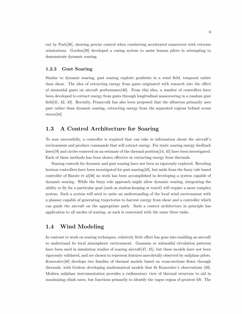
2.1 Autonomous dynamic soaring process. The aircraft starts by flying a mappingpattern (top), enters a dynamic soaring cycle (middle), and updates the trajectoryas the wind map and aircraft speed evolves (bottom). . . . . . . . . . . . . . . . 9
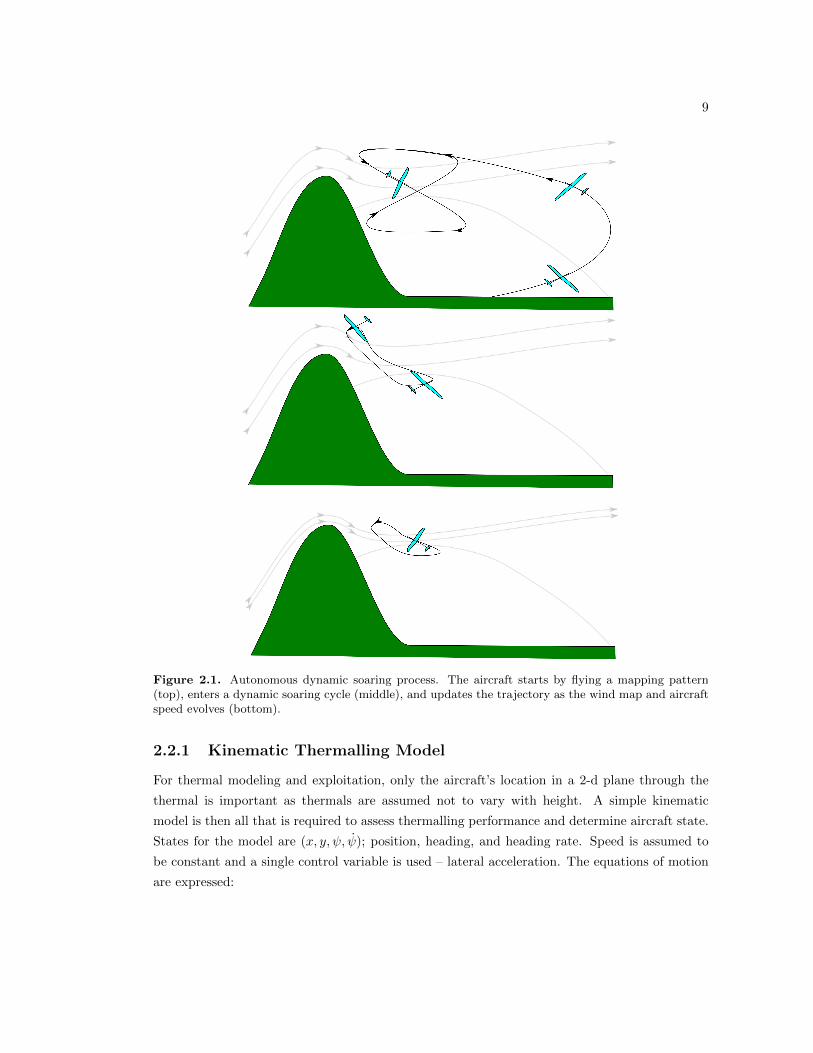
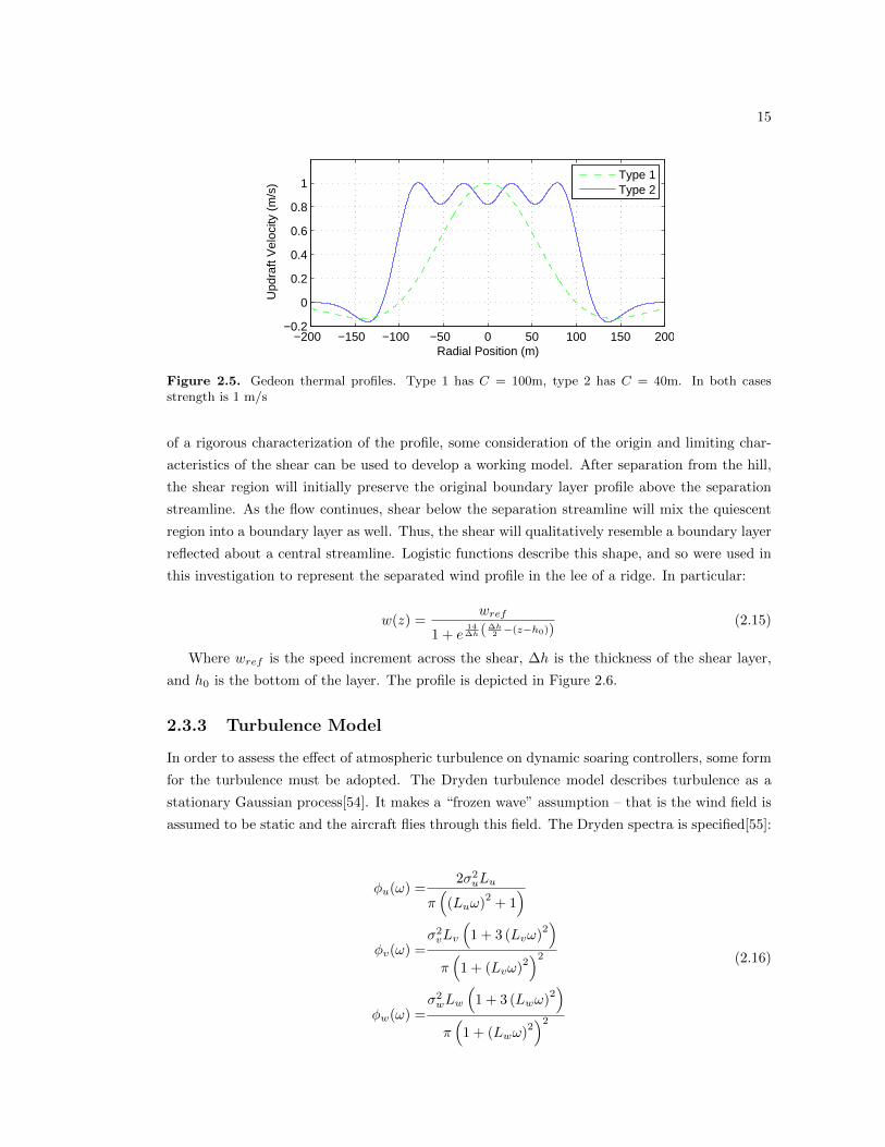
2.2 Coordinate frames used in modeling motion of DS aircraft. . . . . . . . . . . . . 102.3 Fox aircraft flying under power. From the Fox assembly manual[2]. . . . . . . . . 122.4 Performance characteristics of the Escale Fox aircraft. . . . . . . . . . . . . . . . 132.5 Gedeon thermal profiles. Type 1 has C = 100m, type 2 has C = 40m. In both
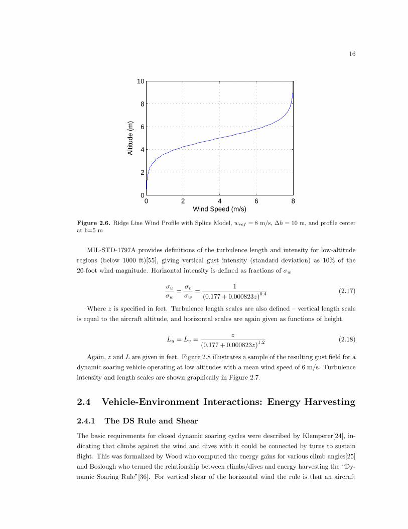
cases strength is 1 m/s . . . . . . . . . . . . . . . . . . . . . . . . . . . . . . . . . 152.6 Ridge Line Wind Profile with Spline Model, wref = 8 m/s, ∆h = 10 m, and
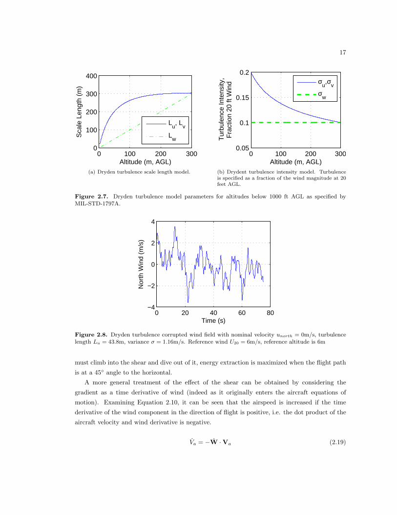
profile center at h=5 m . . . . . . . . . . . . . . . . . . . . . . . . . . . . . . . . 162.7 Dryden turbulence model parameters for altitudes below 1000 ft AGL as specified
by MIL-STD-1797A. . . . . . . . . . . . . . . . . . . . . . . . . . . . . . . . . . . 172.8 Dryden turbulence corrupted wind field with nominal velocity unorth = 0m/s,
turbulence length Lu = 43.8m, variance σ = 1.16m/s. Reference wind U20 =6m/s, reference altitude is 6m . . . . . . . . . . . . . . . . . . . . . . . . . . . . . 17
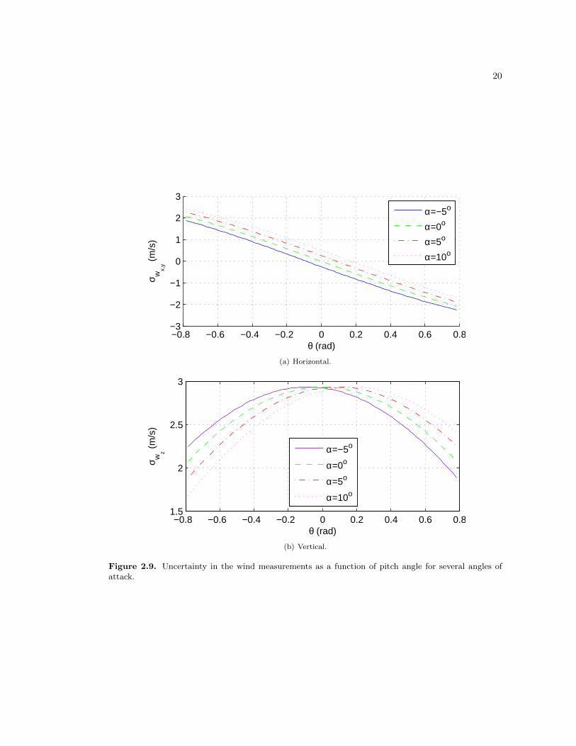
2.9 Uncertainty in the wind measurements as a function of pitch angle for severalangles of attack. . . . . . . . . . . . . . . . . . . . . . . . . . . . . . . . . . . . . 20
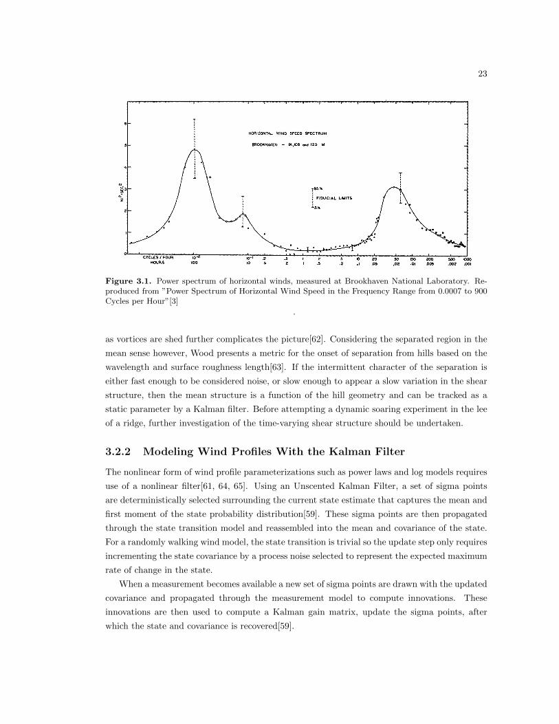
3.1 Power spectrum of horizontal winds, measured at Brookhaven National Labo-ratory. Reproduced from ”Power Spectrum of Horizontal Wind Speed in theFrequency Range from 0.0007 to 900 Cycles per Hour”[3] . . . . . . . . . . . . . 23
3.2 Basis splines and one example spline with knots [0, 0.25, 0.5, 0.75, 1], order 3 . . 263.3 Spline and model determined from boundary layer winds estimated from flight
data during 18 Jan flight test. The aircraft was under manual control so the flightpath was highly erratic, contributing to the noise seen in the wind measurements 28
vii
3.4 Wind map estimates and 3 − σ confidence bounds for a 500 run Monte Carlosimulation series. Each run flies the same trajectory and is seeded with a randomturbulence value of mean U20 = 9 m/s and covariance of 3 m/s. All simulationsare run with a shear of 6 m/s located between 100 m and 105 m, the true shearis indicated with thick lines. . . . . . . . . . . . . . . . . . . . . . . . . . . . . . . 30
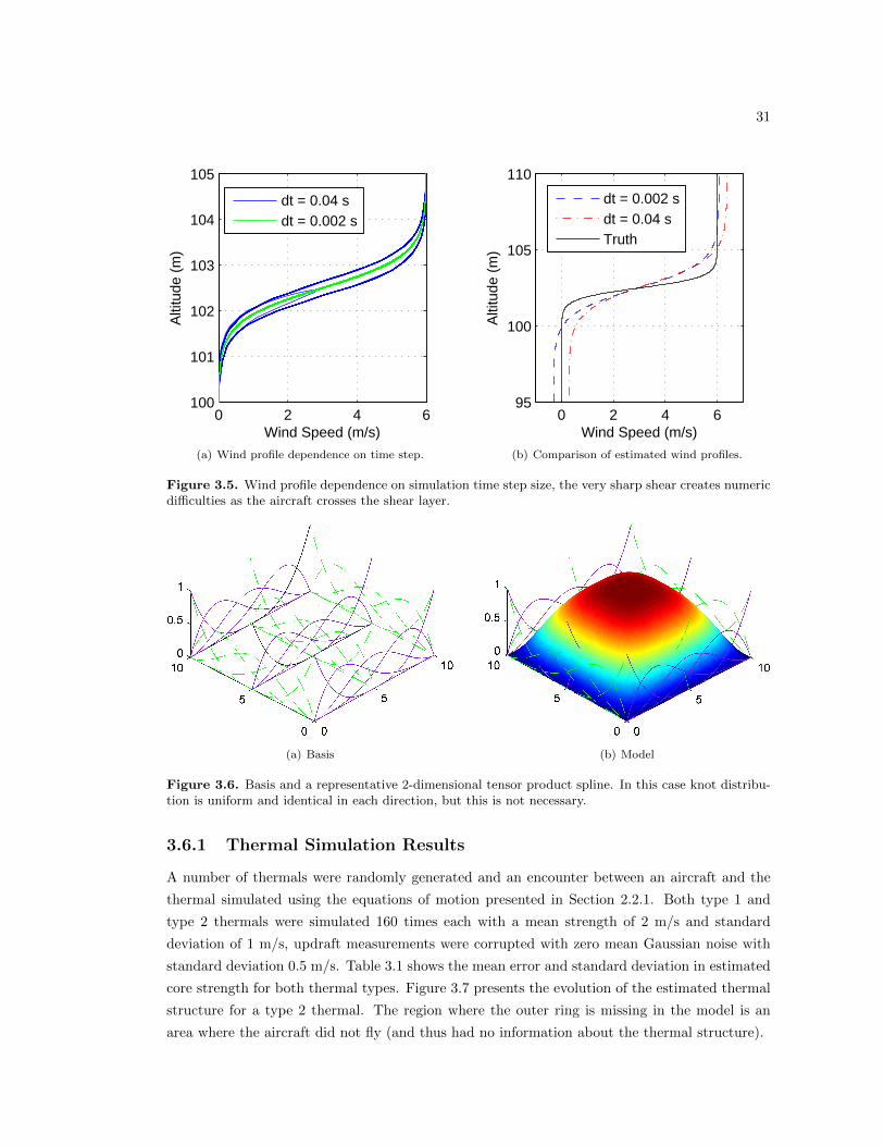
3.5 Wind profile dependence on simulation time step size, the very sharp shear createsnumeric difficulties as the aircraft crosses the shear layer. . . . . . . . . . . . . . 31
3.6 Basis and a representative 2-dimensional tensor product spline. In this case knotdistribution is uniform and identical in each direction, but this is not necessary. . 31
3.7 Evolution of the thermal map for a type 2 thermal w0 = 4.4 m/s, C = 42.93 m.Breaks in the outer ring are in regions not sampled by the sailplane. . . . . . . . 32
4.1 Contours at several levels, illustrating the evolution of trajectory planning atseveral levels. The red trajectory is optimal at an airspeed of 14.8 m/s andachieves a mean climb rate of 0.86 m/s. . . . . . . . . . . . . . . . . . . . . . . . 35
4.2 Illustration of Nonlinear guidance law from Park, et al . . . . . . . . . . . . . . . 354.3 Park’s Nonlinear Guidance Law Modified for Circular Trajectories . . . . . . . . 364.4 Flight paths for three thermalling techniques during a four minute simulation of
an encounter with a type 1 thermal C0 = 3.2 m/s, R = 114.46 m. Thermal centeris located at (0, 0). . . . . . . . . . . . . . . . . . . . . . . . . . . . . . . . . . . . 38
4.5 Climb rate during first and last 60 seconds of simulation in type 1 thermal. C0 =3.2 m/s, R = 114.46 m. The periodic notch in the planning method climb rateoccurs on replanning as the aircraft maneuvers to intercept the new contour. . . 39
4.6 Flight paths for three thermalling techniques during a four minute simulation ofan encounter with a type 2 thermal C0 = 4.4 m/s, R = 42.93 m. Thermal centeris located at (0, 0). . . . . . . . . . . . . . . . . . . . . . . . . . . . . . . . . . . . 40
4.7 Climb rate during first and last 60 seconds of simulation in type 2 thermal. C0 =4.4 m/s, R = 42.93 m. . . . . . . . . . . . . . . . . . . . . . . . . . . . . . . . . . 41
5.1 Closed loop dynamic soaring system components and communications pathways. 435.2 Feedforward-feedback control structure for dynamic soaring . . . . . . . . . . . . 455.3 Illustration of the Geometry of the Nonlinear Guidance Law . . . . . . . . . . . . 465.4 Dynamic soaring environment illustrating nominal flight path and acceleration,
aircraft pose, and commands (exaggerated for clarity). Flight path is 55 secondsof simulation with shear thickness of 5 m, magnitude of 6 m/s, and no turbulence. 50
5.5 Nominal and actual state history for one dynamic soaring cycle. Cycle is plannedto start at 24.8m/s in shear with ∆h = 5m, w = 6m/s and no turbulence.. . . . . 51
5.6 Flight path consistency measures, RMS error and energy change between adjacentcycles. Error is computed as the minimum distance between the aircraft locationand a point on the flight path, RMS values are computed with a 1000 point slidingwindow. Simulation is initialized with ∆z = 10 m, w=9 m/s with no turbulence.At approximately t=600 seconds, light turbulence is turned on. . . . . . . . . . . 52
5.7 Time histories of wind map parameters for ∆z = 5 m, w=6 m/s, shear center isat 102.5 m. Turbulence is turned on at approx 650 seconds. Occasional spikescan be seen that appear to originate in the inter-process communication. Datastarts when the dynamic soaring initialization command is issued and does notshow wind map convergence prior to start. . . . . . . . . . . . . . . . . . . . . . . 53
viii
List of Tables
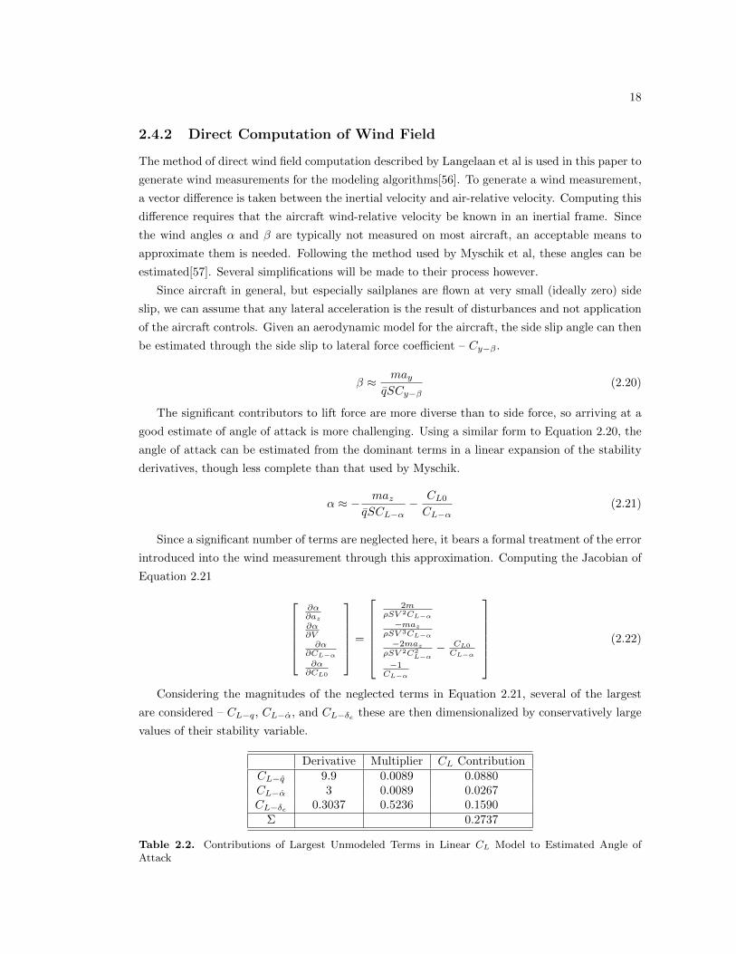
2.1 Fox geometric and mass parameters. . . . . . . . . . . . . . . . . . . . . . . . . . 142.2 Contributions of Largest Unmodeled Terms in Linear CL Model to Estimated
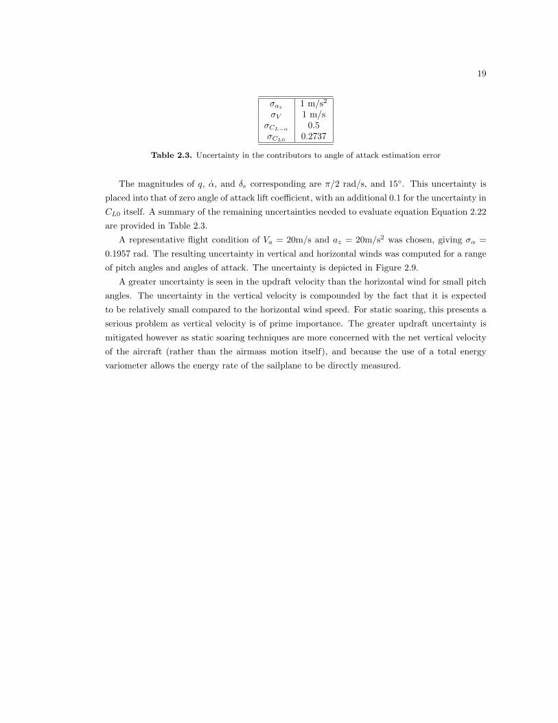
Angle of Attack . . . . . . . . . . . . . . . . . . . . . . . . . . . . . . . . . . . . . 182.3 Uncertainty in the contributors to angle of attack estimation error . . . . . . . . 19
3.1 2-D spline modeling errors from Monte-Carlo simulations. Each thermal type wassimulated in 160 trials, some runs were excluded because the thermal core wasvery weak (less than 1 m/s) or because the aircraft failed to intercept the thermal. 32
4.1 Seed values used in generating thermals. Type 2 thermal radii refer to the radiusof a single core (out of four). . . . . . . . . . . . . . . . . . . . . . . . . . . . . . 37
4.2 Parameters for a simplified performance model of the RnR products SBXC sailplane. 374.3 Results for thermal exploitation of a type 1 thermal. . . . . . . . . . . . . . . . . 384.4 Results for thermal exploitation of type 2 thermals, averaged over 160 simulations. 39
5.1 Wind and turbulence simulation conditions used to test the DS controller, thecenter fields indicate the 20 foot wind parameter used to seed the turbulencemagnitude. To vary turbulence independently of the shear strength, the 20 footwind is treated solely as a turbulence parameter, not as a wind speed. . . . . . . 48
5.2 Dynamic soaring system performance with no turbulence. The 12 m/s conditiontypically failed after the Piccolo attitude filter diverged. (*–the wind map did notreach the convergence criterion and DS was started manually) . . . . . . . . . . . 49
5.3 Dryden parameters for light turbulence. . . . . . . . . . . . . . . . . . . . . . . . 505.4 Dynamic soaring system performance in light turbulence. The 12 m/s condition
typically failed after the Piccolo attitude filter diverged. In 20 m shear the aircraftwas not able to fly any energy-positive cycles at 6 and 9 m/s and could notmaintain flight for more than a few cycles. . . . . . . . . . . . . . . . . . . . . . . 52
ix
Acknowledgments
Corey Montella at Lehigh University was instrumental to this work, generating the trajectoriesand writing the backbone software to allow communication between the wind mapper, controller,and the Piccolo itself.
The support of my advisor, Jack Langelaan, has be phenomenal. Throughout this work,his insights have helped me to move forward on problems and understand both the problemsI faced and occasionally the solutions I’d developed but not fully understood. From his initialtask to develop the wind mapper, I’ve discovered an interest in autonomous exploration of theatmosphere.
In its entirety, the staff of the AVIA lab has made the transition to graduate school and toPenn State a joy. In particular Nate Depenbusch and Sean Quinn Marlow have made my tenurea success, their insights and periodic excitement about some piece of this work has kept fresh theexcitement of studying soaring flight.
x

Dedication
for all the birds who have taught me to fly
xi
Chapter 1Energy Harvesting for Small
Uninhabited Aerial Systems
1.1 Intelligent Systems in Resource-Constrained Applica-
tions
Originally deployed by military organizations, uninhabited aerial systems (uas) are now be-
ing employed in such diverse roles as wildlife monitoring[4], agriculture[5], and severe weather
surveillance[6, 7]. While there remain regulatory and infrastructure barriers to widespread civil-
lian adoption of uas, balancing cost and capability is a significant obstacle. One of the primary
draws of uninhabited systems is the long-endurance missions made possible when an operator
change is as easy as switching desks. Unfortunately the range and endurance required for many
of these missions exceeds the capabilities of many small uas, and in any case a trade must be
made between sensing systems and fuel or batteries. Energy harvesting as a means to extend
capability solely through intelligent control and exploitation of natural atmospheric phenomena
is an attractive means to improve uas capability.
Many of the applications that could benefit most from uas are also very cost-sensitive, pre-
cluding procurement of traditional high-capability aircraft which often have unit costs in excess
of $100 000 [8]. In order to contain costs these applications require aircraft, typically battery
powered, bearing a strong resemblance in size and construction to model aircraft. Indeed, initial
demonstrations of uas use in many applications have used modified RC aircraft[4]. Such aircraft
typically are very limited in endurance, often to less than 15 minutes. Use of intelligent systems
to improve the performance of these systems could potentially allow dramatic improvements in
performance while keeping procurement costs attainable for a variety of innovative applications.
2
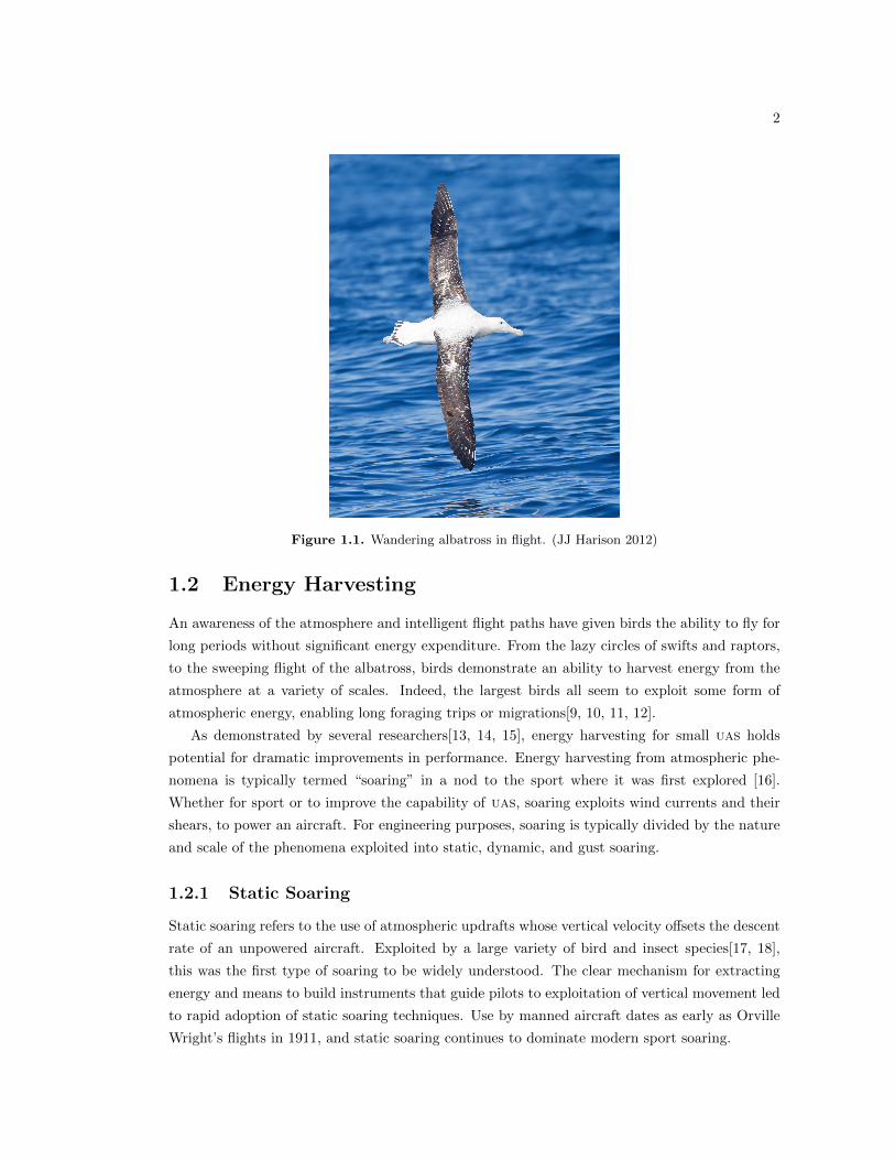
Figure 1.1. Wandering albatross in flight. (JJ Harison 2012)
1.2 Energy Harvesting
An awareness of the atmosphere and intelligent flight paths have given birds the ability to fly for
long periods without significant energy expenditure. From the lazy circles of swifts and raptors,
to the sweeping flight of the albatross, birds demonstrate an ability to harvest energy from the
atmosphere at a variety of scales. Indeed, the largest birds all seem to exploit some form of
atmospheric energy, enabling long foraging trips or migrations[9, 10, 11, 12].
As demonstrated by several researchers[13, 14, 15], energy harvesting for small uas holds
potential for dramatic improvements in performance. Energy harvesting from atmospheric phe-
nomena is typically termed “soaring” in a nod to the sport where it was first explored [16].
Whether for sport or to improve the capability of uas, soaring exploits wind currents and their
shears, to power an aircraft. For engineering purposes, soaring is typically divided by the nature
and scale of the phenomena exploited into static, dynamic, and gust soaring.
1.2.1 Static Soaring
Static soaring refers to the use of atmospheric updrafts whose vertical velocity offsets the descent
rate of an unpowered aircraft. Exploited by a large variety of bird and insect species[17, 18],
this was the first type of soaring to be widely understood. The clear mechanism for extracting
energy and means to build instruments that guide pilots to exploitation of vertical movement led
to rapid adoption of static soaring techniques. Use by manned aircraft dates as early as Orville
Wright’s flights in 1911, and static soaring continues to dominate modern sport soaring.
3
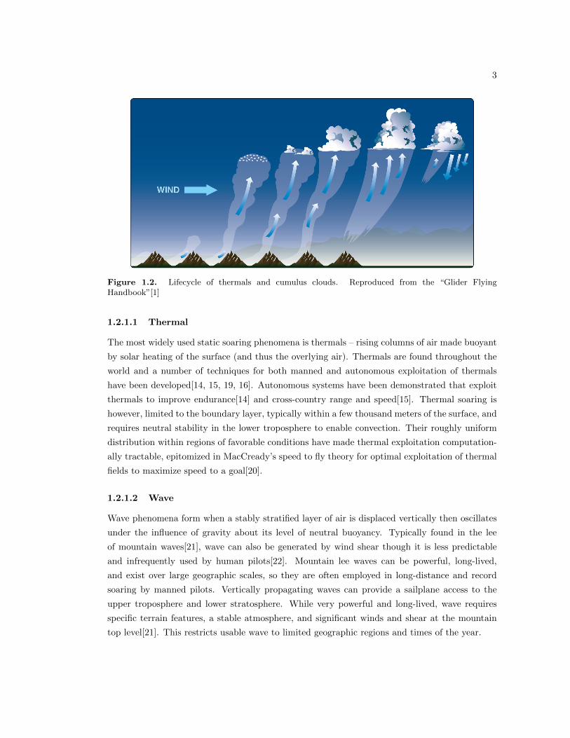
Figure 1.2. Lifecycle of thermals and cumulus clouds. Reproduced from the “Glider FlyingHandbook”[1]
1.2.1.1 Thermal
The most widely used static soaring phenomena is thermals – rising columns of air made buoyant
by solar heating of the surface (and thus the overlying air). Thermals are found throughout the
world and a number of techniques for both manned and autonomous exploitation of thermals
have been developed[14, 15, 19, 16]. Autonomous systems have been demonstrated that exploit
thermals to improve endurance[14] and cross-country range and speed[15]. Thermal soaring is
however, limited to the boundary layer, typically within a few thousand meters of the surface, and
requires neutral stability in the lower troposphere to enable convection. Their roughly uniform
distribution within regions of favorable conditions have made thermal exploitation computation-
ally tractable, epitomized in MacCready’s speed to fly theory for optimal exploitation of thermal
fields to maximize speed to a goal[20].
1.2.1.2 Wave
Wave phenomena form when a stably stratified layer of air is displaced vertically then oscillates
under the influence of gravity about its level of neutral buoyancy. Typically found in the lee
of mountain waves[21], wave can also be generated by wind shear though it is less predictable
and infrequently used by human pilots[22]. Mountain lee waves can be powerful, long-lived,
and exist over large geographic scales, so they are often employed in long-distance and record
soaring by manned pilots. Vertically propagating waves can provide a sailplane access to the
upper troposphere and lower stratosphere. While very powerful and long-lived, wave requires
specific terrain features, a stable atmosphere, and significant winds and shear at the mountain
top level[21]. This restricts usable wave to limited geographic regions and times of the year.
4
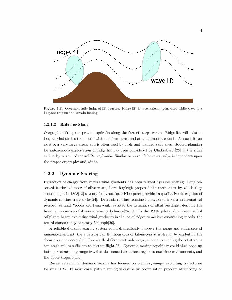
Figure 1.3. Orographically induced lift sources. Ridge lift is mechanically generated while wave is abuoyant response to terrain forcing
1.2.1.3 Ridge or Slope
Orographic lifting can provide updrafts along the face of steep terrain. Ridge lift will exist as
long as wind strikes the terrain with sufficient speed and at an appropriate angle. As such, it can
exist over very large areas, and is often used by birds and manned sailplanes. Routed planning
for autonomous exploitation of ridge lift has been considered by Chakrabarty[23] in the ridge
and valley terrain of central Pennsylvania. Similar to wave lift however, ridge is dependent upon
the proper orography and winds.
1.2.2 Dynamic Soaring
Extraction of energy from spatial wind gradients has been termed dynamic soaring. Long ob-
served in the behavior of albatrosses, Lord Rayleigh proposed the mechanism by which they
sustain flight in 1898[18] seventy-five years later Klemperer provided a qualitative description of
dynamic soaring trajectories[24]. Dynamic soaring remained unexplored from a mathematical
perspective until Woods and Pennycuik revisited the dynamics of albatross flight, deriving the
basic requirements of dynamic soaring behavior[25, 9]. In the 1980s pilots of radio-controlled
sailplanes began exploiting wind gradients in the lee of ridges to achieve astonishing speeds, the
record stands today at nearly 500 mph[26].
A reliable dynamic soaring system could dramatically improve the range and endurance of
unmanned aircraft, the albatross can fly thousands of kilometers at a stretch by exploiting the
shear over open ocean[10]. In a wildly different altitude range, shear surrounding the jet streams
can reach values sufficient to sustain flight[27]. Dynamic soaring capability could thus open up
both persistent, long range travel of the immediate surface region in maritime environments, and
the upper troposphere.
Recent research in dynamic soaring has focused on planning energy exploiting trajectories
for small uas. In most cases path planning is cast as an optimization problem attempting to
5
VaV'a
ΔVw
Shear Layer
ΔW
ΔW
W1
W2
W1
W2
Shear Layer
Vinertial
Vinertial
V'aVa
ΔW
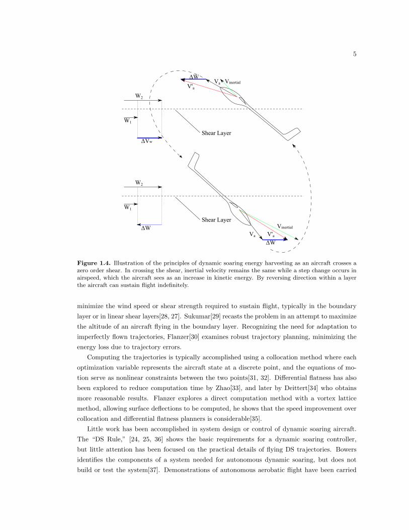
Figure 1.4. Illustration of the principles of dynamic soaring energy harvesting as an aircraft crosses azero order shear. In crossing the shear, inertial velocity remains the same while a step change occurs inairspeed, which the aircraft sees as an increase in kinetic energy. By reversing direction within a layerthe aircraft can sustain flight indefinitely.
minimize the wind speed or shear strength required to sustain flight, typically in the boundary
layer or in linear shear layers[28, 27]. Sukumar[29] recasts the problem in an attempt to maximize
the altitude of an aircraft flying in the boundary layer. Recognizing the need for adaptation to
imperfectly flown trajectories, Flanzer[30] examines robust trajectory planning, minimizing the
energy loss due to trajectory errors.
Computing the trajectories is typically accomplished using a collocation method where each
optimization variable represents the aircraft state at a discrete point, and the equations of mo-
tion serve as nonlinear constraints between the two points[31, 32]. Differential flatness has also
been explored to reduce computation time by Zhao[33], and later by Deittert[34] who obtains
more reasonable results. Flanzer explores a direct computation method with a vortex lattice
method, allowing surface deflections to be computed, he shows that the speed improvement over
collocation and differential flatness planners is considerable[35].
Little work has been accomplished in system design or control of dynamic soaring aircraft.
The “DS Rule,” [24, 25, 36] shows the basic requirements for a dynamic soaring controller,
but little attention has been focused on the practical details of flying DS trajectories. Bowers
identifies the components of a system needed for autonomous dynamic soaring, but does not
build or test the system[37]. Demonstrations of autonomous aerobatic flight have been carried
6
out by Park[38], showing precise control when conducting accelerated maneuvers with extreme
orientations. Gordon[39] developed a cueing system to assist human pilots in attempting to
demonstrate dynamic soaring.
1.2.3 Gust Soaring
Similar to dynamic soaring, gust soaring exploits gradients in a wind field, temporal rather
than shear. The idea of extracting energy from gusts originated with research into the effect
of sinusoidal gusts on aircraft performance[40]. From this idea, a number of controllers have
been developed to extract energy from gusts through longitudinal maneuvering in a random gust
field[41, 42, 43]. Recently, Pennycuik has also been proposed that the albatross primarily uses
gust rather than dynamic soaring, extracting energy from the separated regions behind ocean
waves[44].
1.3 A Control Architecture for Soaring
To soar successfully, a controller is required that can take in information about the aircraft’s
environment and produce commands that will extract energy. For static soaring energy feedback
laws[19] and circles centered on an estimate of the thermal position[14, 45] have been investigated.
Each of these methods has been shown effective in extracting energy from thermals.
Soaring controls for dynamic and gust soaring have not been as rigorously explored. Receding
horizon controllers have been investigated for gust soaring[43], but aside from the fuzzy rule based
controller of Barate et al[46] no work has been accomplished in developing a system capable of
dynamic soaring. While the fuzzy rule approach might allow dynamic soaring, integrating the
ability to fly for a particular goal (such as station-keeping or travel) will require a more complex
system. Such a system will need to unite an understanding of the local wind environment with
a planner capable of generating trajectories to harvest energy from shear and a controller which
can guide the aircraft on the appropriate path. Such a control architecture in principle has
application to all modes of soaring, as each is concerned with the same three tasks.
1.4 Wind Modeling
In contrast to work on soaring techniques, relatively little effort has gone into enabling an aircraft
to understand its local atmospheric environment. Gaussian or solenoidal circulation patterns
have been used in simulation studies of soaring aircraft[47, 45], but these models have not been
rigorously validated, and are chosen to represent features anecdotally observed by sailplane pilots.
Konovalov[48] develops two families of thermal models based on cross-sections flown through
thermals, with Gedeon developing mathematical models that fit Konovalov’s observations [49].
Modern sailplane instrumentation provides a rudimentary view of thermal structure to aid in
maximizing climb rates, but functions primarily to identify the vague region of greatest lift. The
7
controller developed by Allen[14] and extended by Edwards[45] attempts to locate the center of a
thermal by fitting a peak to a sliding window of climb rate measurements, but does not attempt
to identify detailed structures of the windfield.
The literature is similarly sparse in modeling horizontal wind and shear fields. Langelaan[50]
models the boundary layer environment using polynomial functions and a Kalman filter. This
approach demonstrates a degree of modeling skill, but also finds that polynomials do not balance
over fitting and description well, especially for large or complex domains. Bencatel models several
shear environments using particle filters, but does not couple an energy harvesting system[51].
Several wind shear avoidance sensors also provide estimates of the wind shear environment, but
this is limited to simply producing a “hazard index” to ward the pilot of a dangerous condition[52].
1.5 Contributions
This work presents a method to model atmospheric structures and controllers that can be used to
exploit those structures for energy. Atmospheric modeling is presented in the context of mapping
wind fields to support autonomous dynamic soaring and exploitation of thermals. Methods are
presented to model fields with a priori determined structure, as well as arbitrary wind fields.
A candidate controller is presented for exploiting maps of convective updrafts. For dynamic
soaring, a feedforward-feedback architecture is developed to linearize a dynamic soaring trajectory
about a point and fly out path error with a feedback controller. Both applications make use of
a non-linear feedback law for path following[38].
Energy harvesting for both static and dynamic soaring is evaluated in simulation. For dynamic
soaring, a hardware in the loop simulation is used with a commercial off the shelf autopilot to
establish the viability of dynamic soaring with currently available systems.
1.6 Readers Guide
Chapter 2 describes the autonomous dynamic soaring problem and lays out foundational
equations and models for vehicles and the environment that are used throughout this work.
Chapter 3 reviews the mathematics behind the wind models used and describes the wind
modeling systems. Wind mapping results from simulation and flight experiments are pre-
sented, demonstrating the capability of the wind modeling system.
Chapter 4 presents the use of wind maps for static soaring, and a planning method that
exploits wind maps to maximize energy exploitation. Simulation results comparing the
mapping approach to traditional thermalling techniques are shown.
Chapter 5 presents a dynamic soaring system incorporating wind maps, global planners,
and local trajectory control that enables an autonomous aircraft extract energy from wind
shear. Hardware in the loop simulation results demonstrate the capability to dynamic soar
in selected environments.

Chapter 2Vehicle and Environment Models
2.1 Mapping, Planning, and Control for Soaring
The problem of primary interest in this work is the development of a system capable of au-
tonomously dynamic soaring, specifically in the separated flow region behind ridges. The system
should have a number of capabilities.
• Take off with no knowledge of the winds.
• Fly a pattern to gather information on the wind field structure, and identify when sufficient
information has been gathered to begin dynamic soaring.
• Identify a suitable trajectory, enter, and sustain a dynamic soaring cycle in the mapped
shear environment.
• Update the wind map and trajectory while dynamic soaring as more information is gathered
and the wind field evolves.
An illustration of this process is shown in Figure 2.1. While this process is described here
in the context of dynamic soaring, the mapping, exploitation, and replanning cycle is relevant
to any form of atmospheric energy harvesting. Application of this process to static soaring is
also developed and presented. First, the foundational vehicle and environmental models used
throughout this work will be presented.
2.2 Vehicle Model
Several vehicle models were used in a number of simulations. Fidelity ranges from two dimensional
kinematics to a six degree of freedom model using extensive lookup tables for aerodynamic forces
and moments.
9
Figure 2.1. Autonomous dynamic soaring process. The aircraft starts by flying a mapping pattern(top), enters a dynamic soaring cycle (middle), and updates the trajectory as the wind map and aircraftspeed evolves (bottom).
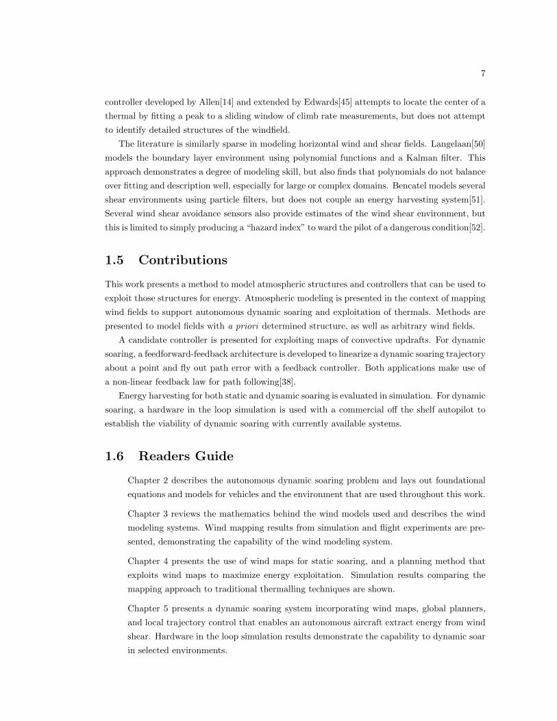
2.2.1 Kinematic Thermalling Model
For thermal modeling and exploitation, only the aircraft’s location in a 2-d plane through the
thermal is important as thermals are assumed not to vary with height. A simple kinematic
model is then all that is required to assess thermalling performance and determine aircraft state.
States for the model are (x, y, ψ, ψ); position, heading, and heading rate. Speed is assumed to
be constant and a single control variable is used – lateral acceleration. The equations of motion
are expressed:
10
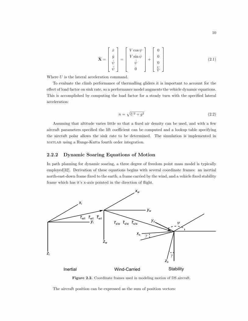
X =
x
y
ψ
ψ
=
V cosψ
V sinψ
ψ
0
+
0
0
0UV
(2.1)
Where U is the lateral acceleration command.
To evaluate the climb performance of thermalling gliders it is important to account for the
effect of load factor on sink rate, so a performance model augments the vehicle dynamic equations.
This is accomplished by computing the load factor for a steady turn with the specified lateral
acceleration:
n =√U2 + g2 (2.2)
Assuming that altitude varies little so that a fixed air density can be used, and with a few
aircraft parameters specified the lift coefficient can be computed and a lookup table specifying
the aircraft polar allows the sink rate to be determined. The simulation is implemented in
matlab using a Runge-Kutta fourth order integration.
2.2.2 Dynamic Soaring Equations of Motion
In path planning for dynamic soaring, a three degree of freedom point mass model is typically
employed[32]. Derivation of these equations begins with several coordinate frames: an inertial
north-east-down frame fixed to the earth, a frame carried by the wind, and a vehicle fixed stability
frame which has it’s x-axis pointed in the direction of flight.
xi
yi
zi
xw
yw
zw
xs
ys
zs
ψ
γ
γ
rw/irw/i rw/irs/wrs/w rs/w
Inertial Wind-Carried Stability
Figure 2.2. Coordinate frames used in modeling motion of DS aircraft.
The aircraft position can be expressed as the sum of position vectors:
11
ris/i = riw/i + ris/w (2.3)
Adopting the notation of Stephens and Lewis[53], wheres∂xta/b∂t indicates the partial derivative
taken in the s frame of the vector x, measured between a and b, whose components are expressed
in the t frame. An inertial derivative with respect to time is taken of the position:
i∂ris/i
∂t= ris/i = ωw/i × riw/i + riw/i + ωs/w × ris/w + ris/w (2.4)
Rewriting riw/i as W, noting that ωw/i = 0 considering an instant where Os and Ow (the
coordinate system origins) are coincident so that ris/w = 0:
ris/i = W + ris/w (2.5)
Taking another derivative:
i∂rs/i
∂t2= ris/i = ωw/i ×W + W + ωs/w × ris/w + ris/w (2.6)
Noting again, that ωw/i = 0 and transforming to stability frame:
Rs/iris/i =
Rs/iF
m= Rs/iW + ωs/w × rss/w + rss/w (2.7)
Where rss/w = [Va, 0, 0]T . Taking the bank angle, µ, to be an input so that it’s dynamics need
not be handled explicitly then Rs/i can be expanded:
Rs/i =
cos γ cosψ cos γ sinψ − sin γ
− sinψ cosψ 0
sin γ cosψ sin γ sinψ cos γ
(2.8)
Rotating the angular velocity ωs/w to stability frame:
ωss/w =
cos γ 0 − sin γ
0 1 0
sin γ 0 cos γ
0
γ
ψ
=
− sin γψ
−γcos γψ
(2.9)
Substituting into Equation 2.7 and expanding the force and wind terms:
−Dm− g sin γ = Va + Wx cos γ cosψ + Wy cos γ sinψ − Wz sin γ
L
msinµ = Vaψ cos γ − Wx sinψ + Wy cosψ
− Lm
cosµ+ g cos γ = −Vaγ + Wx sin γ cosψ + Wy sin γ sinψ + Wz cos γ
(2.10)
12
Assuming that the wind is in the horizontal plane only, and rearranging for the state deriva-
tives:
Va = −d− g sin γ − Wx cos γ cosψ − Wy cos γ sinψ
ψ = l sinµ+ Wx sinψ − Wy cosψ
γ = l cosµ− g cos γ + Wx sin γ cosψ + Wy sin γ sinψ
(2.11)
The navigation equations given in Equation 2.5 can be rewritten in terms of Va, giving:
ris/i =
˙North
˙East
˙Down
=
Wn
We
Wd
+
Va cos γ cosψ
Va cos γ sinψ
−Va sin γ
(2.12)
Equations 2.11 and 2.12 then fully specify the motion of a dynamic soaring aircraft whose
rotational dynamics are assumed to be slow enough to be neglected, and that flies with no
sideslip angle. While restrictive, these assumptions are realistic for ideal DS paths – to maximize
efficiency it is desirable to fly coordinated (i.e. without sideslip), and dynamic soaring paths tend
to be smooth which reduces the effect of the rotational dynamics.
2.2.3 Six Degree of Freedom Model for HiL Simulation
For hardware in the loop simulation, the Piccolo HiL simulation is used. This implements a
six degree of freedom aircraft simulation that runs in real time and allows specification of a
wind profile and aircraft model. The aircraft model is specified using lookup tables for stability
derivatives as a function of angle of attack. Stability axis force coefficients and body axis moment
coefficients are constructed as a function of angle of attack, sideslip, non-dimensional body rates,
and surface deflections. The aircraft dynamics are computed on a spherical Earth and states
communicated to the Piccolo using CAN bus.
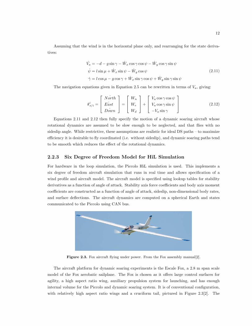
Figure 2.3. Fox aircraft flying under power. From the Fox assembly manual[2].
The aircraft platform for dynamic soaring experiments is the Escale Fox, a 2.8 m span scale
model of the Fox aerobatic sailplane. The Fox is chosen as it offers large control surfaces for
agility, a high aspect ratio wing, auxiliary propulsion system for launching, and has enough
internal volume for the Piccolo and dynamic soaring system. It is of conventional configuration,
with relatively high aspect ratio wings and a cruciform tail, pictured in Figure 2.3[2]. The
13
−5 0 5 10 15−0.1
−0.05
0
0.05
0.1
α (degrees)
−5 0 5 10 15−0.5
0
0.5
1
1.5
Cm
CL
(a) Lift and moment
0 0.5 1 1.5
5
10
15
20
CL
L/D
0 10 20 30 40
0
5
10
15
20
Indicated Airspeed (m/s)
L/D
(b) Drag
0 0.2 0.4 0.6 0.8 1
−0.1
0
0.1
x/c
y/c
(c) Airfoil
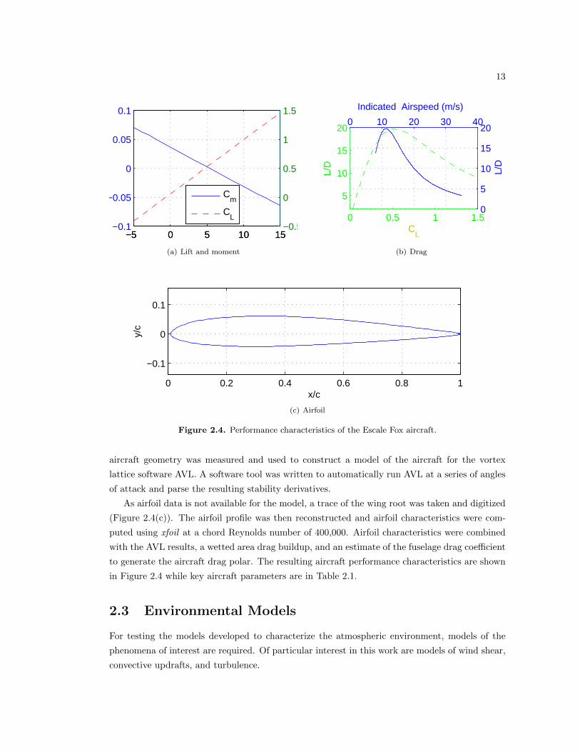
Figure 2.4. Performance characteristics of the Escale Fox aircraft.
aircraft geometry was measured and used to construct a model of the aircraft for the vortex
lattice software AVL. A software tool was written to automatically run AVL at a series of angles
of attack and parse the resulting stability derivatives.
As airfoil data is not available for the model, a trace of the wing root was taken and digitized
(Figure 2.4(c)). The airfoil profile was then reconstructed and airfoil characteristics were com-
puted using xfoil at a chord Reynolds number of 400,000. Airfoil characteristics were combined
with the AVL results, a wetted area drag buildup, and an estimate of the fuselage drag coefficient
to generate the aircraft drag polar. The resulting aircraft performance characteristics are shown
in Figure 2.4 while key aircraft parameters are in Table 2.1.
2.3 Environmental Models
For testing the models developed to characterize the atmospheric environment, models of the
phenomena of interest are required. Of particular interest in this work are models of wind shear,
convective updrafts, and turbulence.
14
Parameter ValueS 0.634 m2
c 0.226 mb 2.8 mm 4 kgJx 0.729 kg-m2
Jy 0.343 kg-m2
Jz 1.07 kg-m2
Jxz 0.0 kg-m2
L/Dmax 19.7
Table 2.1. Fox geometric and mass parameters.
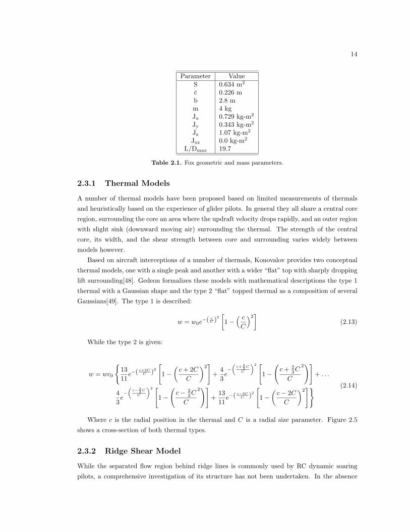
2.3.1 Thermal Models
A number of thermal models have been proposed based on limited measurements of thermals
and heuristically based on the experience of glider pilots. In general they all share a central core
region, surrounding the core an area where the updraft velocity drops rapidly, and an outer region
with slight sink (downward moving air) surrounding the thermal. The strength of the central
core, its width, and the shear strength between core and surrounding varies widely between
models however.
Based on aircraft interceptions of a number of thermals, Konovalov provides two conceptual
thermal models, one with a single peak and another with a wider “flat” top with sharply dropping
lift surrounding[48]. Gedeon formalizes these models with mathematical descriptions the type 1
thermal with a Gaussian shape and the type 2 “flat” topped thermal as a composition of several
Gaussians[49]. The type 1 is described:
w = w0e−( cC )
2[1−
( cC
)2](2.13)
While the type 2 is given:
w = wc0
{13
11e−( c+2C
C )2
[1−
(c+ 2C
C
)2]
+4
3e−(c+ 2
3C
C
)2 [1−
(c+ 2
3C
C
2)]
+ . . .
4
3e−(c− 2
3C
C
)2 [1−
(c− 2
3C
C
2)]
+13
11e−( c−2C
C )2
[1−
(c− 2C
C
)2]} (2.14)
Where c is the radial position in the thermal and C is a radial size parameter. Figure 2.5
shows a cross-section of both thermal types.
2.3.2 Ridge Shear Model
While the separated flow region behind ridge lines is commonly used by RC dynamic soaring
pilots, a comprehensive investigation of its structure has not been undertaken. In the absence
15
−200 −150 −100 −50 0 50 100 150 200−0.2
0
0.2
0.4
0.6
0.8
1
Radial Position (m)
Upd
raft
Vel
ocity
(m
/s)
Type 1Type 2
Figure 2.5. Gedeon thermal profiles. Type 1 has C = 100m, type 2 has C = 40m. In both casesstrength is 1 m/s
of a rigorous characterization of the profile, some consideration of the origin and limiting char-
acteristics of the shear can be used to develop a working model. After separation from the hill,
the shear region will initially preserve the original boundary layer profile above the separation
streamline. As the flow continues, shear below the separation streamline will mix the quiescent
region into a boundary layer as well. Thus, the shear will qualitatively resemble a boundary layer
reflected about a central streamline. Logistic functions describe this shape, and so were used in
this investigation to represent the separated wind profile in the lee of a ridge. In particular:
w(z) =wref
1 + e14∆h ( ∆h
2 −(z−h0))(2.15)
Where wref is the speed increment across the shear, ∆h is the thickness of the shear layer,
and h0 is the bottom of the layer. The profile is depicted in Figure 2.6.
2.3.3 Turbulence Model
In order to assess the effect of atmospheric turbulence on dynamic soaring controllers, some form
for the turbulence must be adopted. The Dryden turbulence model describes turbulence as a
stationary Gaussian process[54]. It makes a “frozen wave” assumption – that is the wind field is
assumed to be static and the aircraft flies through this field. The Dryden spectra is specified[55]:
φu(ω) =2σ2
uLu
π(
(Luω)2
+ 1)
φv(ω) =σ2vLv
(1 + 3 (Lvω)
2)
π(
1 + (Lvω)2)2
φw(ω) =σ2wLw
(1 + 3 (Lwω)
2)
π(
1 + (Lwω)2)2
(2.16)
16
0 2 4 6 80
2
4
6
8
10
Wind Speed (m/s)
Alti
tude
(m
)
Figure 2.6. Ridge Line Wind Profile with Spline Model, wref = 8 m/s, ∆h = 10 m, and profile centerat h=5 m
MIL-STD-1797A provides definitions of the turbulence length and intensity for low-altitude
regions (below 1000 ft)[55], giving vertical gust intensity (standard deviation) as 10% of the
20-foot wind magnitude. Horizontal intensity is defined as fractions of σw
σuσw
=σvσw
=1
(0.177 + 0.000823z)0.4 (2.17)
Where z is specified in feet. Turbulence length scales are also defined – vertical length scale
is equal to the aircraft altitude, and horizontal scales are again given as functions of height.
Lu = Lv =z
(0.177 + 0.000823z)1.2 (2.18)
Again, z and L are given in feet. Figure 2.8 illustrates a sample of the resulting gust field for a
dynamic soaring vehicle operating at low altitudes with a mean wind speed of 6 m/s. Turbulence
intensity and length scales are shown graphically in Figure 2.7.
2.4 Vehicle-Environment Interactions: Energy Harvesting
2.4.1 The DS Rule and Shear
The basic requirements for closed dynamic soaring cycles were described by Klemperer[24], in-
dicating that climbs against the wind and dives with it could be connected by turns to sustain
flight. This was formalized by Wood who computed the energy gains for various climb angles[25]
and Boslough who termed the relationship between climbs/dives and energy harvesting the “Dy-
namic Soaring Rule”[36]. For vertical shear of the horizontal wind the rule is that an aircraft
17
0 100 200 3000
100
200
300
400
Altitude (m, AGL)
Sca
le L
engt
h (m
)
Lu, L
v
Lw
(a) Dryden turbulence scale length model.
0 100 200 3000.05
0.1
0.15
0.2
Altitude (m, AGL)
Tur
bule
nce
Inte
nsity
,F
ract
ion
20 ft
Win
d
σ
u,σ
v
σw
(b) Drydent turbulence intensity model. Turbulenceis specified as a fraction of the wind magnitude at 20feet AGL.
Figure 2.7. Dryden turbulence model parameters for altitudes below 1000 ft AGL as specified byMIL-STD-1797A.
0 20 40 60 80−4
−2
0
2
4
Time (s)
Nor
th W
ind
(m/s
)
Figure 2.8. Dryden turbulence corrupted wind field with nominal velocity unorth = 0m/s, turbulencelength Lu = 43.8m, variance σ = 1.16m/s. Reference wind U20 = 6m/s, reference altitude is 6m
must climb into the shear and dive out of it, energy extraction is maximized when the flight path
is at a 45◦ angle to the horizontal.
A more general treatment of the effect of the shear can be obtained by considering the
gradient as a time derivative of wind (indeed as it originally enters the aircraft equations of
motion). Examining Equation 2.10, it can be seen that the airspeed is increased if the time
derivative of the wind component in the direction of flight is positive, i.e. the dot product of the
aircraft velocity and wind derivative is negative.
Va = −W ·Va (2.19)
18
2.4.2 Direct Computation of Wind Field
The method of direct wind field computation described by Langelaan et al is used in this paper to
generate wind measurements for the modeling algorithms[56]. To generate a wind measurement,
a vector difference is taken between the inertial velocity and air-relative velocity. Computing this
difference requires that the aircraft wind-relative velocity be known in an inertial frame. Since
the wind angles α and β are typically not measured on most aircraft, an acceptable means to
approximate them is needed. Following the method used by Myschik et al, these angles can be
estimated[57]. Several simplifications will be made to their process however.
Since aircraft in general, but especially sailplanes are flown at very small (ideally zero) side
slip, we can assume that any lateral acceleration is the result of disturbances and not application
of the aircraft controls. Given an aerodynamic model for the aircraft, the side slip angle can then
be estimated through the side slip to lateral force coefficient – Cy−β .
β ≈ mayqSCy−β
(2.20)
The significant contributors to lift force are more diverse than to side force, so arriving at a
good estimate of angle of attack is more challenging. Using a similar form to Equation 2.20, the
angle of attack can be estimated from the dominant terms in a linear expansion of the stability
derivatives, though less complete than that used by Myschik.
α ≈ − mazqSCL−α
− CL0CL−α
(2.21)
Since a significant number of terms are neglected here, it bears a formal treatment of the error
introduced into the wind measurement through this approximation. Computing the Jacobian of
Equation 2.21
∂α∂az∂α∂V∂α
∂CL−α∂α∂CL0
=
2m
ρSV 2CL−α−maz
ρSV 3CL−α−2maz
ρSV 2C2L−α− CL0
CL−α
−1CL−α
(2.22)
Considering the magnitudes of the neglected terms in Equation 2.21, several of the largest
are considered – CL−q, CL−α, and CL−δe these are then dimensionalized by conservatively large
values of their stability variable.
Derivative Multiplier CL ContributionCL−q 9.9 0.0089 0.0880CL−α 3 0.0089 0.0267CL−δe 0.3037 0.5236 0.1590
Σ 0.2737
Table 2.2. Contributions of Largest Unmodeled Terms in Linear CL Model to Estimated Angle ofAttack
19
σaz 1 m/s2
σV 1 m/sσCL−α 0.5σCL0
0.2737
Table 2.3. Uncertainty in the contributors to angle of attack estimation error
The magnitudes of q, α, and δe corresponding are π/2 rad/s, and 15◦. This uncertainty is
placed into that of zero angle of attack lift coefficient, with an additional 0.1 for the uncertainty in
CL0 itself. A summary of the remaining uncertainties needed to evaluate equation Equation 2.22
are provided in Table 2.3.
A representative flight condition of Va = 20m/s and az = 20m/s2 was chosen, giving σα =
0.1957 rad. The resulting uncertainty in vertical and horizontal winds was computed for a range
of pitch angles and angles of attack. The uncertainty is depicted in Figure 2.9.
A greater uncertainty is seen in the updraft velocity than the horizontal wind for small pitch
angles. The uncertainty in the vertical velocity is compounded by the fact that it is expected
to be relatively small compared to the horizontal wind speed. For static soaring, this presents a
serious problem as vertical velocity is of prime importance. The greater updraft uncertainty is
mitigated however as static soaring techniques are more concerned with the net vertical velocity
of the aircraft (rather than the airmass motion itself), and because the use of a total energy
variometer allows the energy rate of the sailplane to be directly measured.
20
−0.8 −0.6 −0.4 −0.2 0 0.2 0.4 0.6 0.8−3
−2
−1
0
1
2
3
θ (rad)
σ wx,
y (m
/s)
α=−5o
α=0o
α=5o
α=10o
(a) Horizontal.
−0.8 −0.6 −0.4 −0.2 0 0.2 0.4 0.6 0.81.5
2
2.5
3
θ (rad)
σ wz (
m/s
)
α=−5o
α=0o
α=5o
α=10o
(b) Vertical.
Figure 2.9. Uncertainty in the wind measurements as a function of pitch angle for several angles ofattack.
Chapter 3Wind Mapping
3.1 Kalman Filters, Estimation, and Wind Mapping
Viewing the atmosphere as a dynamic system, then any representation of the wind structure can
be considered simply an expression of the underlying atmospheric state. Different methods of
modeling the wind can be thought of as coordinate transformations of the atmospheric state.
This idea is very powerful and underpins modern data assimilation methods used to combine
atmospheric observations with numerical weather prediction models[58].
In the more restricted case of determining atmospheric wind structure surrounding an air
vehicle, the dynamical system view is equally useful. As a dynamical system, conventional engi-
neering methods to estimate the state of a system can be used, in particular the Kalman filter and
its nonlinear extensions. In its simplest form, the Kalman filter provides the optimal, unbiased
estimate of the state of a linear system subject to Gaussian random process and measurement
noise[59]. Extensions to the Kalman filter allow non-linear systems to be treated, and while they
no longer can claim optimality, experience shows the estimates produced to be very good[59, 60].
3.2 Mapping an a priori Determined Structure
If the shear structure is known a priori to have a structure which can be defined parametrically,
then the estimation problem is reduced simply to a parameter estimation problem – determining
the static (or slowly time-varying) parameters of the wind model.
3.2.1 Variability of the Mean Wind Field
When modeling pre-determined structures, the parameters defining the wind field shape are
treated as slowly varying constants. The validity of this approach bears some consideration for
shears of interest to dynamic soaring.
22
3.2.1.1 Boundary Layer Shear
Considering the diabatic wind profile in the boundary layer[61]:
u =u?κ
[ln
z
z0+ f(z, z0,L)
](3.1)
Where u? =
√(w′u′)0, the surface momentum flux and L is the Monin-Obukhov parameter[61]:
L = − u3?θv
κg(w′θ′v)0(3.2)
With θv the boundary layer virtual potential temperature, κ the von Karman constant and
(w′θ′v)0 is the surface buoyancy flux. The wind profile is a function of:
• Surface momentum flux, a function of the outer flow velocity, determined in the mean by
synoptic and mesoscale forcing.
• Mean boundary layer temperature, determined by the synoptic temperature structure and
diurnal heating.
• Surface buoyancy flux, a function of the stability and diurnal heating.
• Roughness length, a characteristic of the local terrain.
Restricting our consideration to homogenous terrain as complex terrain is unsuitable for
boundary layer dynamic soaring due to the difficulty of assuring terrain separation (not to men-
tion that complex terrain is likely to support other sources of shear or vertical velocity), then the
boundary layer parameters are all functions of synoptic or mesoscale forcing and diurnal heating.
In the absence of discontinuous features such as cold fronts (which are likely to support static
soaring as an alternative), the boundary layer wind profile will then be relatively stable on time
scales between several minutes and several hours. Indeed this is borne out by Van der Hoven’s
study of the spectrum of atmospheric motion[3], reproduced in Figure 3.1.
Convective boundary layers do complicate matter somewhat, as their contribution to wind
variation occurs with a period of several minutes (the second peak in Van der Hoven’s spectrum).
As with fronts, a convective boundary layer supports static soaring, providing greater terrain
clearance and vision range for an aircraft, consequently here it is supposed that dynamic soaring
would only be preferred when no other soaring techniques are available. Considering stable
boundary layers, fluctuations about the mean shear structure can then be interpreted as random
turbulence after the Dryden model[54]. The slow variations of the mean profile can then be
tracked by appropriate selection of the Kalman filter process noise.
3.2.1.2 Ridge Shear
The approach taken for boundary layers is not applicable to ridge shears, as the separated region
is driven by turbulent motion and a non-hydrostatic pressure gradient. Intermittent separation
23
Figure 3.1. Power spectrum of horizontal winds, measured at Brookhaven National Laboratory. Re-produced from ”Power Spectrum of Horizontal Wind Speed in the Frequency Range from 0.0007 to 900Cycles per Hour”[3]
.
as vortices are shed further complicates the picture[62]. Considering the separated region in the
mean sense however, Wood presents a metric for the onset of separation from hills based on the
wavelength and surface roughness length[63]. If the intermittent character of the separation is
either fast enough to be considered noise, or slow enough to appear a slow variation in the shear
structure, then the mean structure is a function of the hill geometry and can be tracked as a
static parameter by a Kalman filter. Before attempting a dynamic soaring experiment in the lee
of a ridge, further investigation of the time-varying shear structure should be undertaken.
3.2.2 Modeling Wind Profiles With the Kalman Filter
The nonlinear form of wind profile parameterizations such as power laws and log models requires
use of a nonlinear filter[61, 64, 65]. Using an Unscented Kalman Filter, a set of sigma points
are deterministically selected surrounding the current state estimate that captures the mean and
first moment of the state probability distribution[59]. These sigma points are then propagated
through the state transition model and reassembled into the mean and covariance of the state.
For a randomly walking wind model, the state transition is trivial so the update step only requires
incrementing the state covariance by a process noise selected to represent the expected maximum
rate of change in the state.
When a measurement becomes available a new set of sigma points are drawn with the updated
covariance and propagated through the measurement model to compute innovations. These
innovations are then used to compute a Kalman gain matrix, update the sigma points, after
which the state and covariance is recovered[59].
24
3.3 Mapping Arbitrary Wind Structures
A pre-specified structure is acceptable for some wind environments and has the strength of al-
lowing a structure to be selected intelligently that captures the essential features of the expected
field. In many cases however, the wind structure is chaotic and a more general solution is needed.
Langelaan et al[50] attempted to model wind shears with polynomial functions. Such functions
demonstrate some skill, but attaining a sufficiently descriptive model without overfitting is chal-
lenging for polynomials. The use of piecewise polynomial splines offers an attractive alternative
to polynomials, allowing complex structures to be represented compactly while reducing the
overfitting seen in high-order polynomials.
3.3.1 Spline Mathematics
At its simplest, a spline is a piecewise polynomial function, and it can be constructed by piecewise
summation of polynomial functions. The nature of a spline can be visualized by dividing the
domain of a function into a set of segments separated by “knots” – points where the kth derivative
of the function is allowed to be discontinuous, with k determining the order of the spline. Owing
to its piecewise nature a spline can be written as a linear combination of simpler functions given
a suitable basis. This form is known as the basis spline (or B-spline) form, and allows the spline
function to be written as a linear mapping[66]:
S(h) =
g+k−1∑i=1
ciNi(h) (3.3)
Where N defines a spline basis supported on the interval defined by knots λj , j = 1..., g and
forms a partition of unity at every point x, λ1 ≤ x ≤ λg. The coefficients, c are the coordinates
specifying a particular function as a linear combination of the basis N . After defining the spline
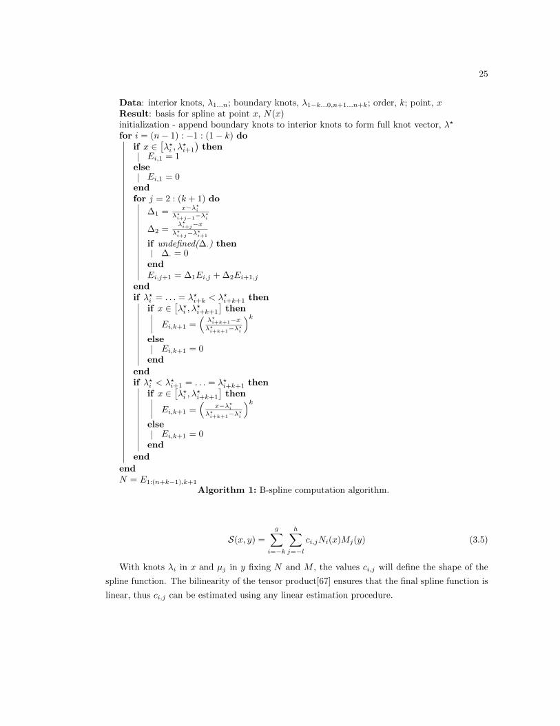
order and knot locations, the value of the spline basis, N , can be determined using a triangular
scheme[66] described in Algorithm 1. The basis spline as a linear combination of simpler functions
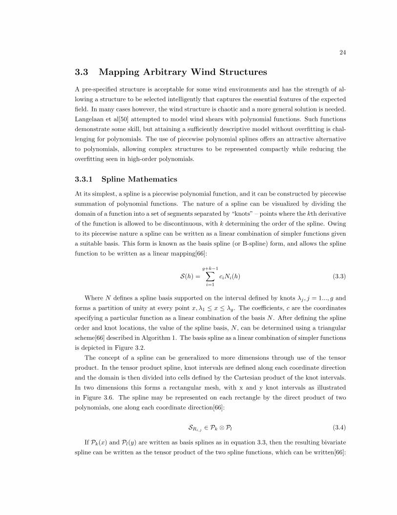
is depicted in Figure 3.2.
The concept of a spline can be generalized to more dimensions through use of the tensor
product. In the tensor product spline, knot intervals are defined along each coordinate direction
and the domain is then divided into cells defined by the Cartesian product of the knot intervals.
In two dimensions this forms a rectangular mesh, with x and y knot intervals as illustrated
in Figure 3.6. The spline may be represented on each rectangle by the direct product of two
polynomials, one along each coordinate direction[66]:
SRi,j ∈ Pk ⊗ Pl (3.4)
If Pk(x) and Pl(y) are written as basis splines as in equation 3.3, then the resulting bivariate
spline can be written as the tensor product of the two spline functions, which can be written[66]:
25
Data: interior knots, λ1...n; boundary knots, λ1−k...0,n+1...n+k; order, k; point, xResult: basis for spline at point x, N(x)initialization - append boundary knots to interior knots to form full knot vector, λ?
for i = (n− 1) : −1 : (1− k) doif x ∈
[λ?i , λ
?i+1
)then
Ei,1 = 1else
Ei,1 = 0endfor j = 2 : (k + 1) do
∆1 =x−λ?i
λ?i+j−1−λ?i
∆2 =λ?i+j−x
λ?i+j−λ?i+1
if undefined(∆·) then∆· = 0
endEi,j+1 = ∆1Ei,j + ∆2Ei+1,j
endif λ?i = . . . = λ?i+k < λ?i+k+1 then
if x ∈[λ?i , λ
?i+k+1
]then
Ei,k+1 =(λ?i+k+1−xλ?i+k+1−λ
?i
)kelse
Ei,k+1 = 0end
endif λ?i < λ?i+1 = . . . = λ?i+k+1 then
if x ∈[λ?i , λ
?i+k+1
]then
Ei,k+1 =(
x−λ?iλ?i+k+1−λ
?i
)kelse
Ei,k+1 = 0end
end
endN = E1:(n+k−1),k+1
Algorithm 1: B-spline computation algorithm.
S(x, y) =
g∑i=−k
h∑j=−l
ci,jNi(x)Mj(y) (3.5)
With knots λi in x and µj in y fixing N and M , the values ci,j will define the shape of the
spline function. The bilinearity of the tensor product[67] ensures that the final spline function is
linear, thus ci,j can be estimated using any linear estimation procedure.
26
0 0.2 0.4 0.6 0.8 10
0.2
0.4
0.6
0.8
1
B−Splines
c=[0,0,1,1,1,0,0]
Knots
Figure 3.2. Basis splines and one example spline with knots [0, 0.25, 0.5, 0.75, 1], order 3
3.3.2 Wind Mapping with Splines
Since the spline S(z) represents a linear mapping, it can be implemented in a Kalman filter to
build a model of the wind environment as measurements of the wind field are taken. The Kalman
filter states form a vector concatenating the spline coordinates in each direction:
X =
cnorth
ceast
cdown
(3.6)
If a model is available for the time evolution of the wind field, it can be used to propagate
the spline coefficients forward in time. Assuming here, that changes in the wind field are small
and random so that the state transition is trivial, the Kalman filter can be constructed with the
prediction step proceeding:
Xt|t−1 = Xt−1|t−1
Pt|t = Pt|t−1 + Qt
(3.7)
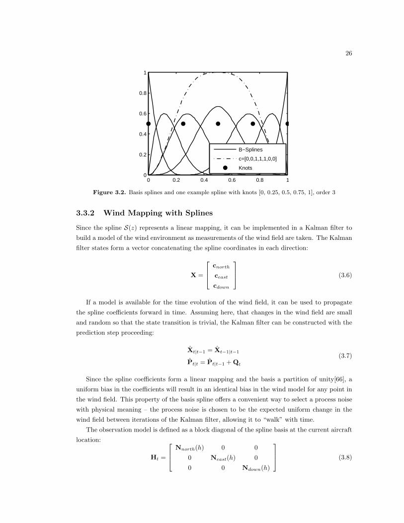
Since the spline coefficients form a linear mapping and the basis a partition of unity[66], a
uniform bias in the coefficients will result in an identical bias in the wind model for any point in
the wind field. This property of the basis spline offers a convenient way to select a process noise
with physical meaning – the process noise is chosen to be the expected uniform change in the
wind field between iterations of the Kalman filter, allowing it to “walk” with time.
The observation model is defined as a block diagonal of the spline basis at the current aircraft
location:
Ht =
Nnorth(h) 0 0
0 Neast(h) 0
0 0 Ndown(h)
(3.8)
27
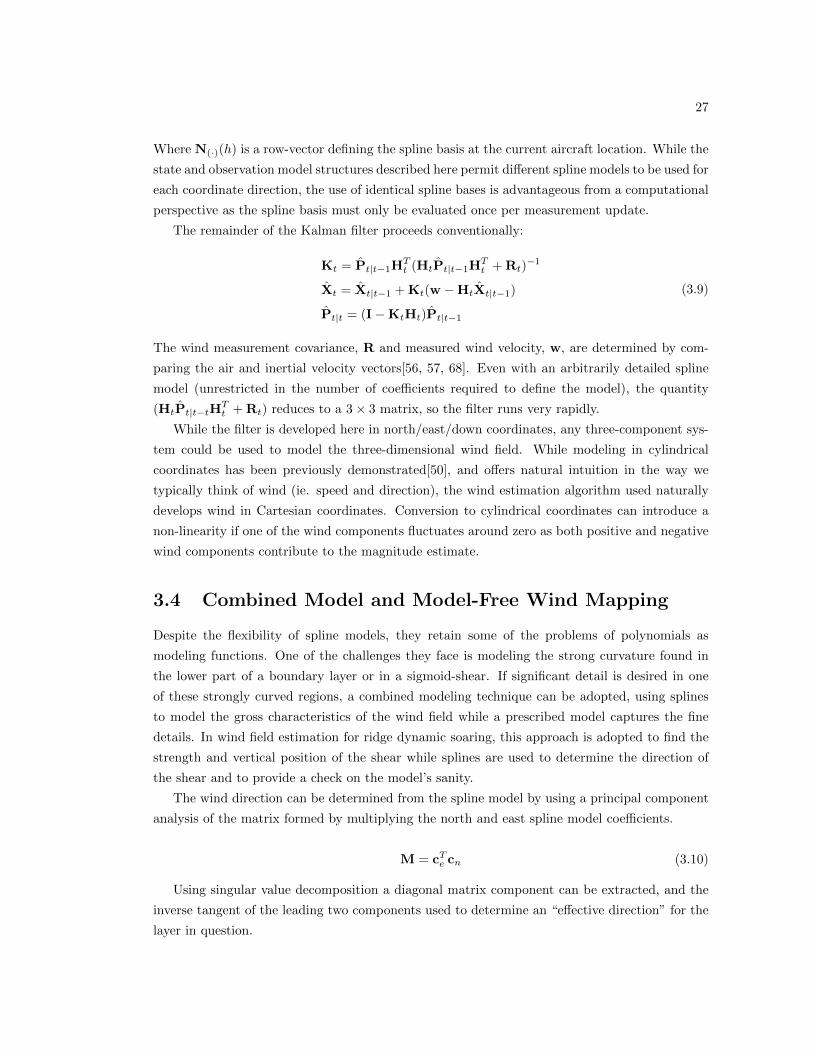
Where N(·)(h) is a row-vector defining the spline basis at the current aircraft location. While the
state and observation model structures described here permit different spline models to be used for
each coordinate direction, the use of identical spline bases is advantageous from a computational
perspective as the spline basis must only be evaluated once per measurement update.
The remainder of the Kalman filter proceeds conventionally:
Kt = Pt|t−1HTt (HtPt|t−1H
Tt + Rt)
−1
Xt = Xt|t−1 + Kt(w −HtXt|t−1)
Pt|t = (I−KtHt)Pt|t−1
(3.9)
The wind measurement covariance, R and measured wind velocity, w, are determined by com-
paring the air and inertial velocity vectors[56, 57, 68]. Even with an arbitrarily detailed spline
model (unrestricted in the number of coefficients required to define the model), the quantity
(HtPt|t−tHTt + Rt) reduces to a 3× 3 matrix, so the filter runs very rapidly.
While the filter is developed here in north/east/down coordinates, any three-component sys-
tem could be used to model the three-dimensional wind field. While modeling in cylindrical
coordinates has been previously demonstrated[50], and offers natural intuition in the way we
typically think of wind (ie. speed and direction), the wind estimation algorithm used naturally
develops wind in Cartesian coordinates. Conversion to cylindrical coordinates can introduce a
non-linearity if one of the wind components fluctuates around zero as both positive and negative
wind components contribute to the magnitude estimate.
3.4 Combined Model and Model-Free Wind Mapping
Despite the flexibility of spline models, they retain some of the problems of polynomials as
modeling functions. One of the challenges they face is modeling the strong curvature found in
the lower part of a boundary layer or in a sigmoid-shear. If significant detail is desired in one
of these strongly curved regions, a combined modeling technique can be adopted, using splines
to model the gross characteristics of the wind field while a prescribed model captures the fine
details. In wind field estimation for ridge dynamic soaring, this approach is adopted to find the
strength and vertical position of the shear while splines are used to determine the direction of
the shear and to provide a check on the model’s sanity.
The wind direction can be determined from the spline model by using a principal component
analysis of the matrix formed by multiplying the north and east spline model coefficients.
M = cTe cn (3.10)
Using singular value decomposition a diagonal matrix component can be extracted, and the
inverse tangent of the leading two components used to determine an “effective direction” for the
layer in question.
28
This technique has the advantage of capturing the direction influence of every layer in the
shear and weighting it appropriately by the wind strength. If a simple low-pass filter is instead
used on the instantaneously measured direction, then the noisy signal in the low-wind section
would impact the wind direction equally to the strong wind above the shear, which is more
important when planning DS paths.
3.5 1-D Mapping Results
The combined modeling method was applied in both simulation and flight tests to test its ability
to map the wind field. Validating a wind model in flight is challenging as high-resolution obser-
vational data is unavailable. A combination of simulation and flights is thus used to establish
the basic validity of the modeling technique.
3.5.1 Simulations
3.5.2 Fox Boundary-Layer Data
During a flight test of the E-Scale Fox, data was recorded at 25Hz from the Piccolo autopilot
and used to drive a boundary-layer modeling wind map. For safety of flight, the aircraft was not
flown in the lower boundary layer so no data was gathered below 40m where the wind profile
exhibits the most curvature. A boundary layer structure is still observed however, the profile
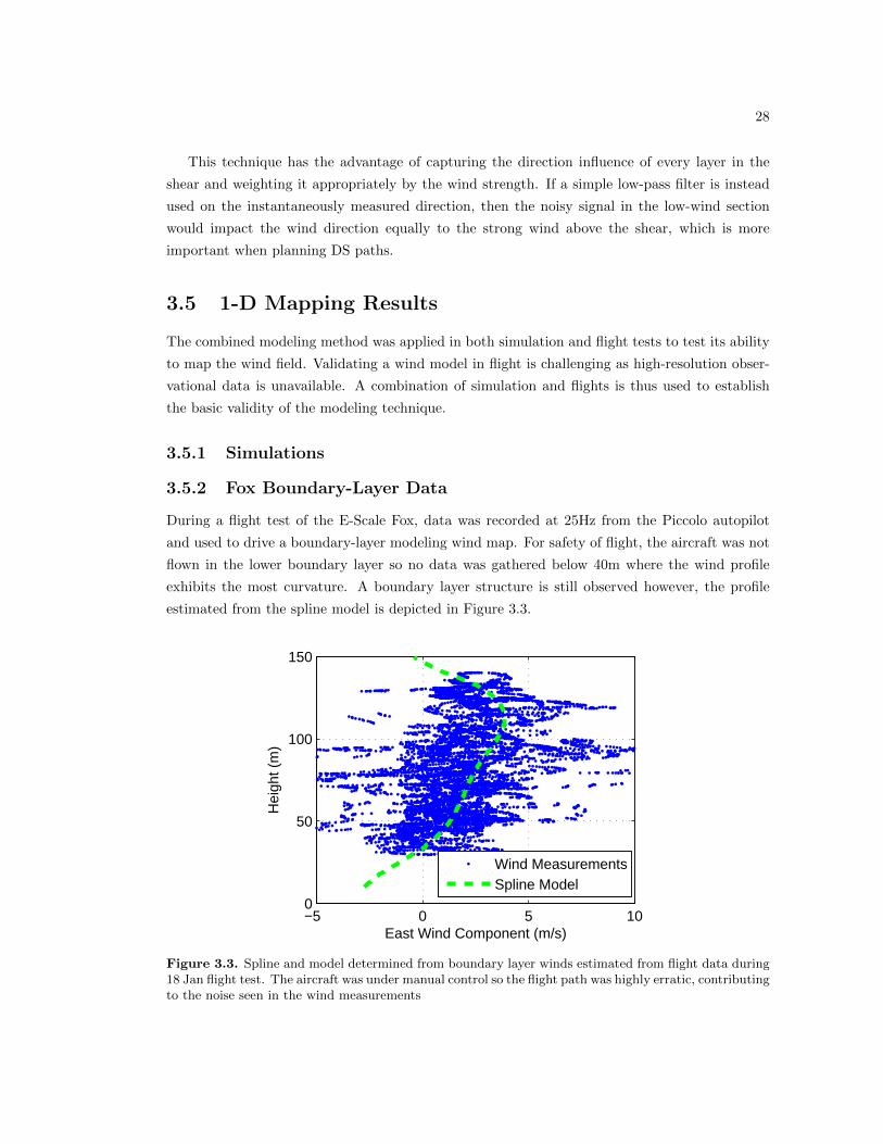
estimated from the spline model is depicted in Figure 3.3.
−5 0 5 100
50
100
150
Hei
ght (
m)
East Wind Component (m/s)
Wind MeasurementsSpline Model
Figure 3.3. Spline and model determined from boundary layer winds estimated from flight data during18 Jan flight test. The aircraft was under manual control so the flight path was highly erratic, contributingto the noise seen in the wind measurements
29
3.5.3 Ridge Shear Modeling Simulation
To test the combined model and model free approach, a simulation of an aircraft dynamic soaring
in the lee of a ridge is used. The simulation is implemented in matlab using the equations of
motion developed in Section 2.2.2 and the aircraft performance model from Section 2.2.3. The
aircraft is initialized at the surface, climbs to intercept a shear at h=100 m and then begins
dynamic soaring. Since the intent is to test the wind mapper in dynamic soaring, the controller
is given the wind profile a priori and in addition to the controller discussed in Section 5.4 it is
equipped with direct thrust and CL control to ensure it flies the proper dynamic soaring path.
A 500 run Monte Carlo simulation is used to diagnose the reliability of the wind mapping
method. The wind map is initialized with the shear bottom at 95 m, a thickness of 30 m, and a
shear strength of 8 m/s. Environmental conditions locate the shear at h=100 m, a thickness of
5 m, and strength of 6 m/s. Process noise is set in the Kalman filters to allow the shear to drift
by 1 m/s in magnitude and 1 m of location and thickness per 100 seconds. The simulations were
conducted with Dryden turbulence of random amplitude with a mean 20 foot wind parameter of
9 m/s and standard deviation of 3 m/s.
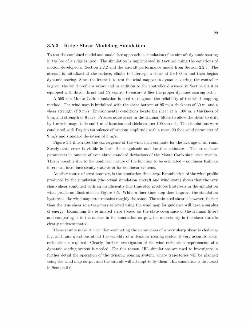
Figure 3.4 illustrates the convergence of the wind field estimate for the average of all runs.
Steady-state error is visible in both the magnitude and location estimates. The true shear
parameters lie outside of even three standard deviations of the Monte Carlo simulation results.
This is possibly due to the nonlinear nature of the function to be estimated – nonlinear Kalman
filters can introduce steady-state error for nonlinear systems.
Another source of error however, is the simulation time step. Examination of the wind profile
produced by the simulation (the actual simulation aircraft and wind state) shows that the very
sharp shear combined with an insufficiently fine time step produces hysteresis in the simulation
wind profile as illustrated in Figure 3.5. While a finer time step does improve the simulation
hysteresis, the wind map error remains roughly the same. The estimated shear is however, thicker
than the true shear so a trajectory selected using the wind map for guidance will have a surplus
of energy. Examining the estimated error (based on the state covariance of the Kalman filter)
and comparing it to the scatter in the simulation output, the uncertainty in the shear state is
clearly underestimated.
These results make it clear that estimating the parameters of a very sharp shear is challeng-
ing, and raise questions about the viability of a dynamic soaring system if very accurate shear
estimation is required. Clearly, further investigation of the wind estimation requirements of a
dynamic soaring system is needed. For this reason, HiL simulations are used to investigate in
further detail the operation of the dynamic soaring system, where trajectories will be planned
using the wind map output and the aircraft will attempt to fly them. HiL simulation is discussed
in Section 5.6.
30
0 50 100 150 20080
90
100
110
120
Time (s)
Alti
tude
(m
)
(a) Estimated top and bottom of shear layer, with 3−σuncertainty bounds from Monte Carlo simulation.
100 150 20095
100
105
110
Time (s)
Alti
tude
(m
)
(b) Shear layer extent, zoom of final 100 seconds ofsimulation.
0 50 100 150 20080
90
100
110
120
Time (s)
Alti
tude
(m
)
(c) Estimated top and bottom of shear layer, uncer-tainty estimated from filter covariance.
0 50 100 150 2004
5
6
7
8
Time (s)
She
ar (
m/s
)
(d) Estimated shear magnitude, with 3−σ uncertaintybounds from Monte Carlo simulation.
Figure 3.4. Wind map estimates and 3 − σ confidence bounds for a 500 run Monte Carlo simulationseries. Each run flies the same trajectory and is seeded with a random turbulence value of mean U20 =9 m/s and covariance of 3 m/s. All simulations are run with a shear of 6 m/s located between 100 mand 105 m, the true shear is indicated with thick lines.
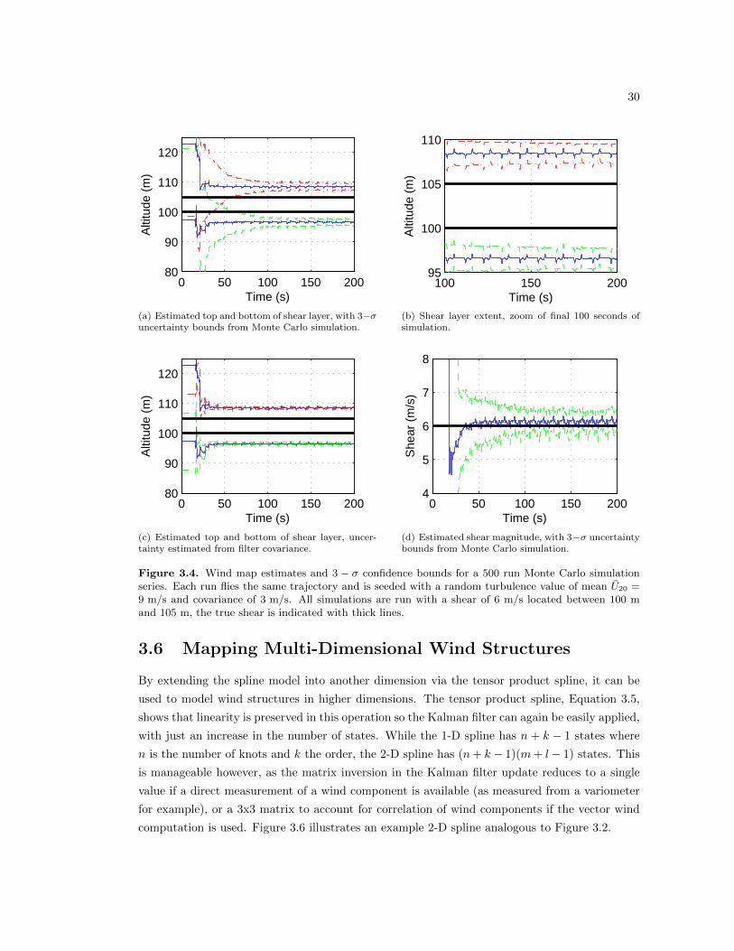
3.6 Mapping Multi-Dimensional Wind Structures
By extending the spline model into another dimension via the tensor product spline, it can be
used to model wind structures in higher dimensions. The tensor product spline, Equation 3.5,
shows that linearity is preserved in this operation so the Kalman filter can again be easily applied,
with just an increase in the number of states. While the 1-D spline has n + k − 1 states where
n is the number of knots and k the order, the 2-D spline has (n+ k − 1)(m+ l− 1) states. This
is manageable however, as the matrix inversion in the Kalman filter update reduces to a single
value if a direct measurement of a wind component is available (as measured from a variometer
for example), or a 3x3 matrix to account for correlation of wind components if the vector wind
computation is used. Figure 3.6 illustrates an example 2-D spline analogous to Figure 3.2.
31
0 2 4 6100
101
102
103
104
105
Wind Speed (m/s)
Alti
tude
(m
)
dt = 0.04 sdt = 0.002 s
(a) Wind profile dependence on time step.
0 2 4 695
100
105
110
Wind Speed (m/s)
Alti
tude
(m
)
dt = 0.002 sdt = 0.04 sTruth
(b) Comparison of estimated wind profiles.
Figure 3.5. Wind profile dependence on simulation time step size, the very sharp shear creates numericdifficulties as the aircraft crosses the shear layer.
(a) Basis (b) Model
Figure 3.6. Basis and a representative 2-dimensional tensor product spline. In this case knot distribu-tion is uniform and identical in each direction, but this is not necessary.
3.6.1 Thermal Simulation Results
A number of thermals were randomly generated and an encounter between an aircraft and the
thermal simulated using the equations of motion presented in Section 2.2.1. Both type 1 and
type 2 thermals were simulated 160 times each with a mean strength of 2 m/s and standard
deviation of 1 m/s, updraft measurements were corrupted with zero mean Gaussian noise with
standard deviation 0.5 m/s. Table 3.1 shows the mean error and standard deviation in estimated
core strength for both thermal types. Figure 3.7 presents the evolution of the estimated thermal
structure for a type 2 thermal. The region where the outer ring is missing in the model is an
area where the aircraft did not fly (and thus had no information about the thermal structure).
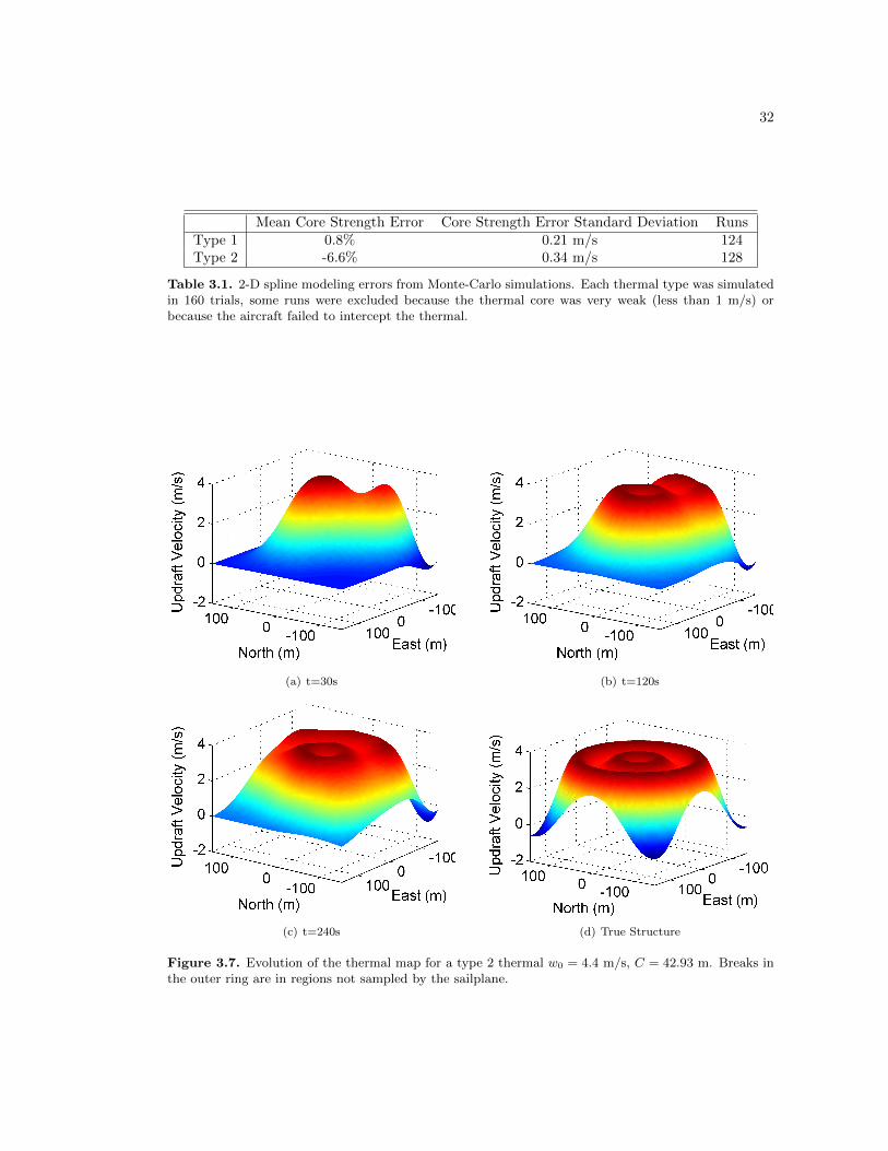
32
Mean Core Strength Error Core Strength Error Standard Deviation RunsType 1 0.8% 0.21 m/s 124Type 2 -6.6% 0.34 m/s 128
Table 3.1. 2-D spline modeling errors from Monte-Carlo simulations. Each thermal type was simulatedin 160 trials, some runs were excluded because the thermal core was very weak (less than 1 m/s) orbecause the aircraft failed to intercept the thermal.
(a) t=30s (b) t=120s
(c) t=240s (d) True Structure
Figure 3.7. Evolution of the thermal map for a type 2 thermal w0 = 4.4 m/s, C = 42.93 m. Breaks inthe outer ring are in regions not sampled by the sailplane.
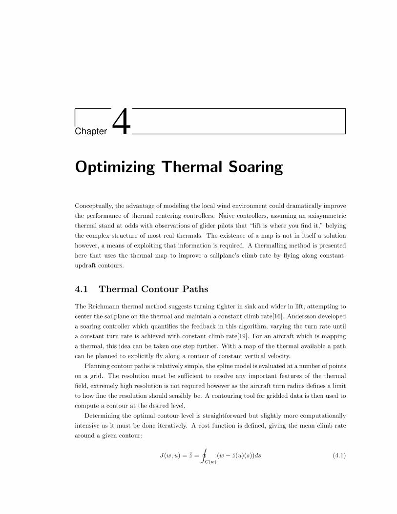
Chapter 4Optimizing Thermal Soaring
Conceptually, the advantage of modeling the local wind environment could dramatically improve
the performance of thermal centering controllers. Naive controllers, assuming an axisymmetric
thermal stand at odds with observations of glider pilots that “lift is where you find it,” belying
the complex structure of most real thermals. The existence of a map is not in itself a solution
however, a means of exploiting that information is required. A thermalling method is presented
here that uses the thermal map to improve a sailplane’s climb rate by flying along constant-
updraft contours.
4.1 Thermal Contour Paths
The Reichmann thermal method suggests turning tighter in sink and wider in lift, attempting to
center the sailplane on the thermal and maintain a constant climb rate[16]. Andersson developed
a soaring controller which quantifies the feedback in this algorithm, varying the turn rate until
a constant turn rate is achieved with constant climb rate[19]. For an aircraft which is mapping
a thermal, this idea can be taken one step further. With a map of the thermal available a path
can be planned to explicitly fly along a contour of constant vertical velocity.
Planning contour paths is relatively simple, the spline model is evaluated at a number of points
on a grid. The resolution must be sufficient to resolve any important features of the thermal
field, extremely high resolution is not required however as the aircraft turn radius defines a limit
to how fine the resolution should sensibly be. A contouring tool for gridded data is then used to
compute a contour at the desired level.
Determining the optimal contour level is straightforward but slightly more computationally
intensive as it must be done iteratively. A cost function is defined, giving the mean climb rate
around a given contour:
J(w, u) = ¯z =
∮C(w)
(w − z(u)(s))ds (4.1)
34
If the aircraft is assumed to be in steady level flight, then the sink rate, z(u), can be computed
easily from the polar, speed, and turn radius. The turn radius is computed at each point on the
trajectory by fitting a circular arc to the point of interest and two points each preceding and
following (five points in total), allowing the load factor to be computed:
n =
√(acg
)2
+ 1 =
√(u
gR
)2
+ 1 (4.2)
The required lift coefficient can then be computed by the conventional definition, with L =
mgn. The speed is treated as an optimization variable, constant for each contour level. The sink
rate can then be computed from the drag polar:
z(u) =ρu3CD(CL)S
2mg(4.3)
Where CD(CL) indicates that the drag coefficient is computed as a function of CL. The
aircraft is numerically “flown” around a candidate trajectory and the difference between the sink
rate on each segment and contour level is integrated to compute the climb in a circuit. The
total climb is divided by the time required to fly a contour, determining the mean climb rate. A
nonlinear optimization routine can then be used to compute the optimal contour level and speed.
In addition to exploiting the aircraft model and the thermal map information, this approach
offers a natural way to deal with complex thermal structures. To account for the effect of complex
thermal geometries which have multiple cores or concave shapes along a contour, the convex hull
of contours of a given level is also considered as a valid path. This allows the aircraft to consider
thermals with multiple cores not large or strong enough to circle singly. Figure 4.1 illustrates
the evolution of a trajectory through several iterations.
This planning method does suffer from the quandary inherent in simultaneous mapping and
exploitation of any resource – insufficient mapping of the wind field potentially leaves an area un-
explored which could improve climb rate, but a thorough exploration takes time which degrades
average climb rate. In an attempt to balance these competing objectives, a dither is applied to
the aircraft goal location’s radial distance from the path centroid. In this investigation a sinu-
soidally varying dither is applied with amplitude of 20 meters and period of 15 seconds. A dither
amplitude based on the local uncertainty in the thermal map may deliver higher performance,
but a fixed dither is used here for simplicity. This dither allows the aircraft to explore a region
close to the current trajectory.
4.2 Closed-loop Control
With a path defined, a controller is needed to keep the aircraft following the desired contour.
The controller used here is a high level controller, developed under the assumption that lower
level control (roll angle, airspeed control, etc) is already provided for on the uas platform. The
controller implemented in this investigation is developed from the guidance method presented by
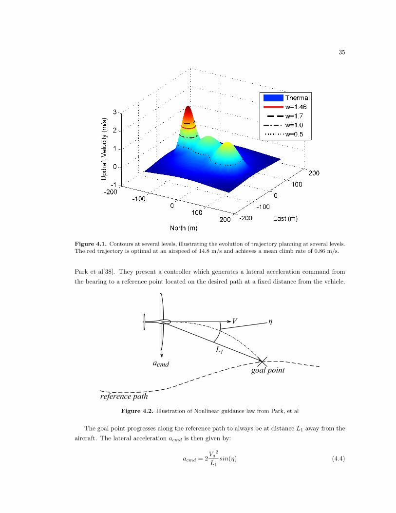
35
Figure 4.1. Contours at several levels, illustrating the evolution of trajectory planning at several levels.The red trajectory is optimal at an airspeed of 14.8 m/s and achieves a mean climb rate of 0.86 m/s.
Park et al[38]. They present a controller which generates a lateral acceleration command from
the bearing to a reference point located on the desired path at a fixed distance from the vehicle.
L1
V
acmd
reference path
goal point
η
Figure 4.2. Illustration of Nonlinear guidance law from Park, et al
The goal point progresses along the reference path to always be at distance L1 away from the
aircraft. The lateral acceleration acmd is then given by:
acmd = 2Va
2
L1sin(η) (4.4)
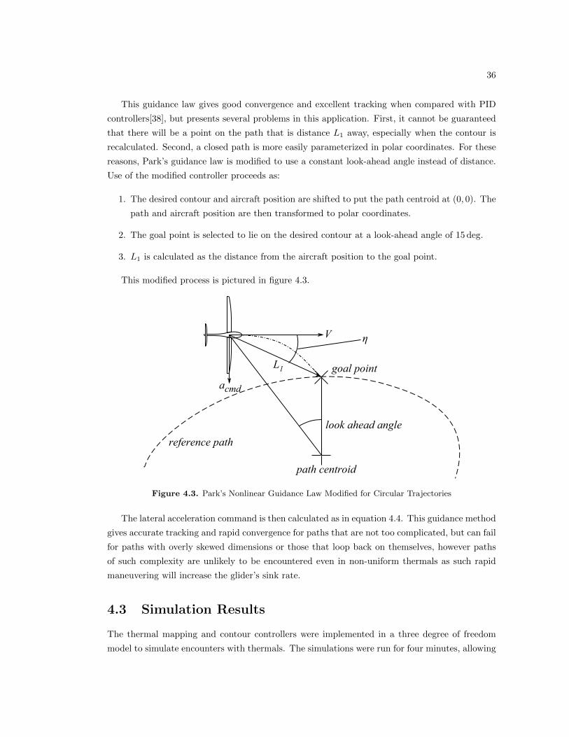
36
This guidance law gives good convergence and excellent tracking when compared with PID
controllers[38], but presents several problems in this application. First, it cannot be guaranteed
that there will be a point on the path that is distance L1 away, especially when the contour is
recalculated. Second, a closed path is more easily parameterized in polar coordinates. For these
reasons, Park’s guidance law is modified to use a constant look-ahead angle instead of distance.
Use of the modified controller proceeds as:
1. The desired contour and aircraft position are shifted to put the path centroid at (0, 0). The
path and aircraft position are then transformed to polar coordinates.
2. The goal point is selected to lie on the desired contour at a look-ahead angle of 15 deg.
3. L1 is calculated as the distance from the aircraft position to the goal point.
This modified process is pictured in figure 4.3.
L1
V
acmd
reference path
goal point
η
path centroid
look ahead angle
Figure 4.3. Park’s Nonlinear Guidance Law Modified for Circular Trajectories
The lateral acceleration command is then calculated as in equation 4.4. This guidance method
gives accurate tracking and rapid convergence for paths that are not too complicated, but can fail
for paths with overly skewed dimensions or those that loop back on themselves, however paths
of such complexity are unlikely to be encountered even in non-uniform thermals as such rapid
maneuvering will increase the glider’s sink rate.
4.3 Simulation Results
The thermal mapping and contour controllers were implemented in a three degree of freedom
model to simulate encounters with thermals. The simulations were run for four minutes, allowing
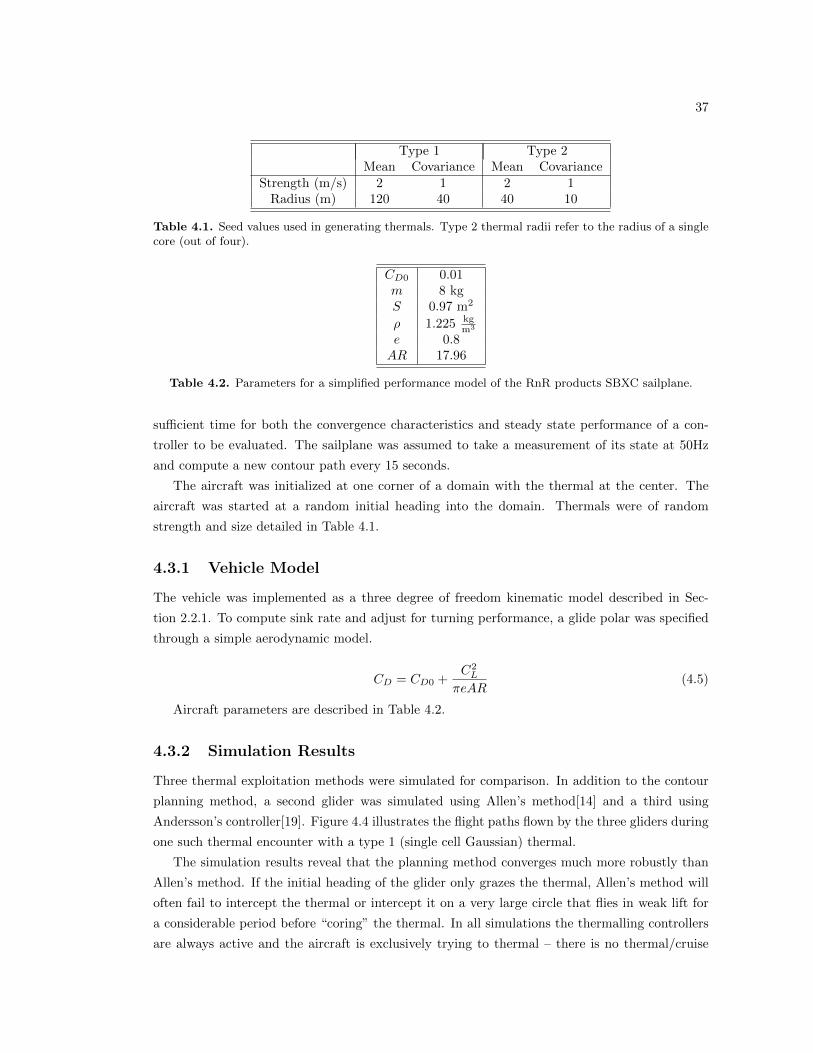
37
Type 1 Type 2Mean Covariance Mean Covariance
Strength (m/s) 2 1 2 1Radius (m) 120 40 40 10
Table 4.1. Seed values used in generating thermals. Type 2 thermal radii refer to the radius of a singlecore (out of four).
CD0 0.01m 8 kgS 0.97 m2
ρ 1.225 kgm3
e 0.8AR 17.96
Table 4.2. Parameters for a simplified performance model of the RnR products SBXC sailplane.
sufficient time for both the convergence characteristics and steady state performance of a con-
troller to be evaluated. The sailplane was assumed to take a measurement of its state at 50Hz
and compute a new contour path every 15 seconds.
The aircraft was initialized at one corner of a domain with the thermal at the center. The
aircraft was started at a random initial heading into the domain. Thermals were of random
strength and size detailed in Table 4.1.
4.3.1 Vehicle Model
The vehicle was implemented as a three degree of freedom kinematic model described in Sec-
tion 2.2.1. To compute sink rate and adjust for turning performance, a glide polar was specified
through a simple aerodynamic model.
CD = CD0 +C2L
πeAR(4.5)
Aircraft parameters are described in Table 4.2.
4.3.2 Simulation Results
Three thermal exploitation methods were simulated for comparison. In addition to the contour
planning method, a second glider was simulated using Allen’s method[14] and a third using
Andersson’s controller[19]. Figure 4.4 illustrates the flight paths flown by the three gliders during
one such thermal encounter with a type 1 (single cell Gaussian) thermal.
The simulation results reveal that the planning method converges much more robustly than
Allen’s method. If the initial heading of the glider only grazes the thermal, Allen’s method will
often fail to intercept the thermal or intercept it on a very large circle that flies in weak lift for
a considerable period before “coring” the thermal. In all simulations the thermalling controllers
are always active and the aircraft is exclusively trying to thermal – there is no thermal/cruise
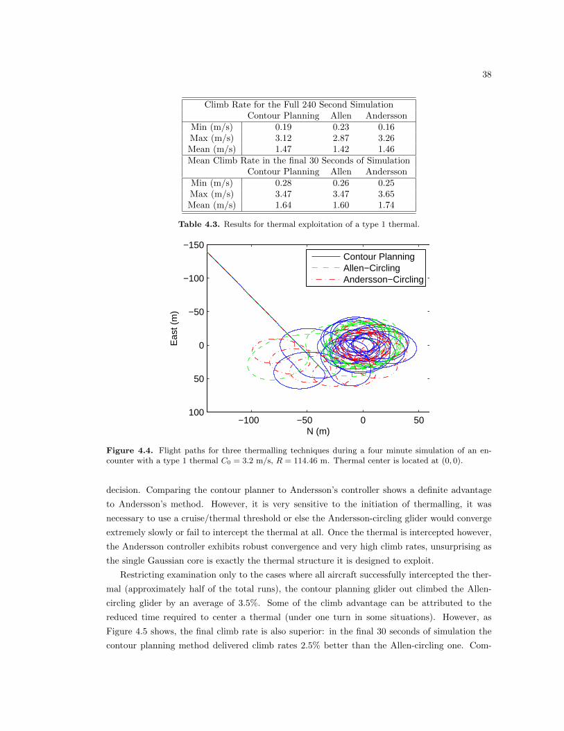
38
Climb Rate for the Full 240 Second SimulationContour Planning Allen Andersson
Min (m/s) 0.19 0.23 0.16Max (m/s) 3.12 2.87 3.26Mean (m/s) 1.47 1.42 1.46Mean Climb Rate in the final 30 Seconds of Simulation
Contour Planning Allen AnderssonMin (m/s) 0.28 0.26 0.25Max (m/s) 3.47 3.47 3.65Mean (m/s) 1.64 1.60 1.74
Table 4.3. Results for thermal exploitation of a type 1 thermal.
−100 −50 0 50
−150
−100
−50
0
50
100
Eas
t (m
)
N (m)
Contour PlanningAllen−CirclingAndersson−Circling
Figure 4.4. Flight paths for three thermalling techniques during a four minute simulation of an en-counter with a type 1 thermal C0 = 3.2 m/s, R = 114.46 m. Thermal center is located at (0, 0).
decision. Comparing the contour planner to Andersson’s controller shows a definite advantage
to Andersson’s method. However, it is very sensitive to the initiation of thermalling, it was
necessary to use a cruise/thermal threshold or else the Andersson-circling glider would converge
extremely slowly or fail to intercept the thermal at all. Once the thermal is intercepted however,
the Andersson controller exhibits robust convergence and very high climb rates, unsurprising as
the single Gaussian core is exactly the thermal structure it is designed to exploit.
Restricting examination only to the cases where all aircraft successfully intercepted the ther-
mal (approximately half of the total runs), the contour planning glider out climbed the Allen-
circling glider by an average of 3.5%. Some of the climb advantage can be attributed to the
reduced time required to center a thermal (under one turn in some situations). However, as
Figure 4.5 shows, the final climb rate is also superior: in the final 30 seconds of simulation the
contour planning method delivered climb rates 2.5% better than the Allen-circling one. Com-
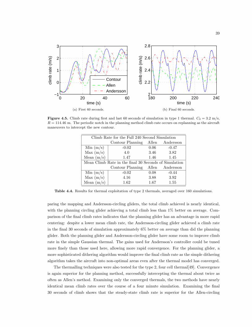
39
0 20 40 60−1
0
1
2
3
time (s)
clim
b ra
te (
m/s
)
ContourAllenAndersson
(a) First 60 seconds.
180 200 220 2402
2.2
2.4
2.6
2.8
time (s)
clim
b ra
te (
m/s
)
(b) Final 60 seconds.
Figure 4.5. Climb rate during first and last 60 seconds of simulation in type 1 thermal. C0 = 3.2 m/s,R = 114.46 m. The periodic notch in the planning method climb rate occurs on replanning as the aircraftmaneuvers to intercept the new contour.
Climb Rate for the Full 240 Second SimulationContour Planning Allen Andersson
Min (m/s) -0.02 0.06 -0.47Max (m/s) 4.0 3.46 3.82Mean (m/s) 1.47 1.46 1.45Mean Climb Rate in the final 30 Seconds of Simulation
Contour Planning Allen AnderssonMin (m/s) -0.02 0.08 -0.44Max (m/s) 4.16 3.88 3.92Mean (m/s) 1.62 1.67 1.55
Table 4.4. Results for thermal exploitation of type 2 thermals, averaged over 160 simulations.
paring the mapping and Andersson-circling gliders, the total climb achieved is nearly identical,
with the planning circling glider achieving a total climb less than 1% better on average. Com-
parison of the final climb rates indicates that the planning glider has an advantage in more rapid
centering: despite a lower mean climb rate, the Andersson-circling glider achieved a climb rate
in the final 30 seconds of simulation approximately 6% better on average than did the planning
glider. Both the planning glider and Andersson-circling glider have some room to improve climb
rate in the simple Gaussian thermal. The gains used for Andersson’s controller could be tuned
more finely than those used here, allowing more rapid convergence. For the planning glider, a
more sophisticated dithering algorithm would improve the final climb rate as the simple dithering
algorithm takes the aircraft into non-optimal areas even after the thermal model has converged.
The thermalling techniques were also tested for the type 2, four cell thermal[49]. Convergence
is again superior for the planning method, successfully intercepting the thermal about twice as
often as Allen’s method. Examining only the converged thermals, the two methods have nearly
identical mean climb rates over the course of a four minute simulation. Examining the final
30 seconds of climb shows that the steady-state climb rate is superior for the Allen-circling
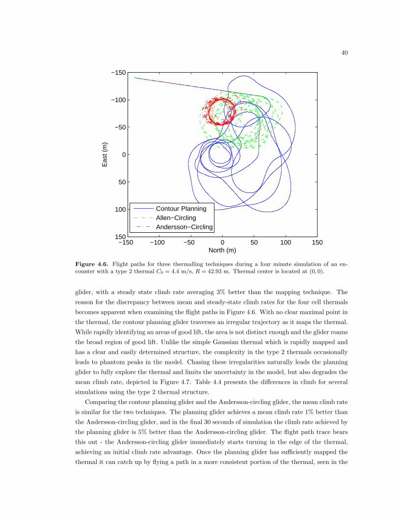
40
−150 −100 −50 0 50 100 150
−150
−100
−50
0
50
100
150
North (m)
Eas
t (m
)
Contour PlanningAllen−CirclingAndersson−Circling
Figure 4.6. Flight paths for three thermalling techniques during a four minute simulation of an en-counter with a type 2 thermal C0 = 4.4 m/s, R = 42.93 m. Thermal center is located at (0, 0).
glider, with a steady state climb rate averaging 3% better than the mapping technique. The
reason for the discrepancy between mean and steady-state climb rates for the four cell thermals
becomes apparent when examining the flight paths in Figure 4.6. With no clear maximal point in
the thermal, the contour planning glider traverses an irregular trajectory as it maps the thermal.
While rapidly identifying an areas of good lift, the area is not distinct enough and the glider roams
the broad region of good lift. Unlike the simple Gaussian thermal which is rapidly mapped and
has a clear and easily determined structure, the complexity in the type 2 thermals occasionally
leads to phantom peaks in the model. Chasing these irregularities naturally leads the planning
glider to fully explore the thermal and limits the uncertainty in the model, but also degrades the
mean climb rate, depicted in Figure 4.7. Table 4.4 presents the differences in climb for several
simulations using the type 2 thermal structure.
Comparing the contour planning glider and the Andersson-circling glider, the mean climb rate
is similar for the two techniques. The planning glider achieves a mean climb rate 1% better than
the Andersson-circling glider, and in the final 30 seconds of simulation the climb rate achieved by
the planning glider is 5% better than the Andersson-circling glider. The flight path trace bears
this out - the Andersson-circling glider immediately starts turning in the edge of the thermal,
achieving an initial climb rate advantage. Once the planning glider has sufficiently mapped the
thermal it can catch up by flying a path in a more consistent portion of the thermal, seen in the
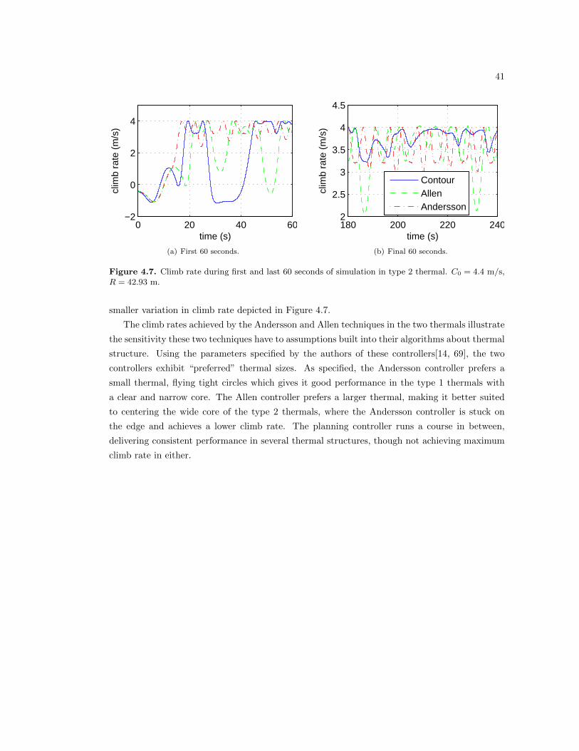
41
0 20 40 60−2
0
2
4cl
imb
rate
(m
/s)
time (s)
(a) First 60 seconds.
180 200 220 2402
2.5
3
3.5
4
4.5
time (s)
clim
b ra
te (
m/s
)
ContourAllenAndersson
(b) Final 60 seconds.
Figure 4.7. Climb rate during first and last 60 seconds of simulation in type 2 thermal. C0 = 4.4 m/s,R = 42.93 m.
smaller variation in climb rate depicted in Figure 4.7.
The climb rates achieved by the Andersson and Allen techniques in the two thermals illustrate
the sensitivity these two techniques have to assumptions built into their algorithms about thermal
structure. Using the parameters specified by the authors of these controllers[14, 69], the two
controllers exhibit “preferred” thermal sizes. As specified, the Andersson controller prefers a
small thermal, flying tight circles which gives it good performance in the type 1 thermals with
a clear and narrow core. The Allen controller prefers a larger thermal, making it better suited
to centering the wide core of the type 2 thermals, where the Andersson controller is stuck on
the edge and achieves a lower climb rate. The planning controller runs a course in between,
delivering consistent performance in several thermal structures, though not achieving maximum
climb rate in either.
Chapter 5Dynamic Soaring
While practiced by birds and RC sailplane pilots, dynamic soaring has thus far proved too
complex for autonomous systems. As dynamic soaring is equally dependent on understanding
the shear environment, planning trajectories, and controlling the vehicle, a complex system is
required for its autonomous realization. Approaches taken to providing for the environmental
information, decision, and control of the vehicle are presented here. A hardware in the loop
simulation is used to establish the viability of the system running on commercially available
hardware.
5.1 Dynamic Soaring at Ridges
For initial investigations into dynamic soaring, the separated region in the lee of a ridge line
provides an attractive environment. Very strong shear exists along the separation streamline,
and has been exploited by RC pilots to fly at speeds nearing 500 mph[26]. As important as
the strength of the shear is the relatively obstruction-free environment. Dynamic soaring in a
boundary layer (“albatross style”) requires very precise maneuvering, as the strongest shear is
closest to the surface. In the case of a ridge line, the high-energy, downward traveling portion of
the dynamic soaring cycle is also taking the aircraft “downhill” so the terrain falls away from the
aircraft. The increased room for maneuvering provides a more forgiving environment for initial
dynamic soaring investigations.
5.2 Control Architecture
The dynamic soaring system consists of the wind mapper discussed in Section 3.4, a global
planner to select the required trajectory, a local planner to fly the trajectory (described in Sec-
tion 5.4), the inter-process communications structure to pass data between the components, and
a communications nexus which sends and receives data from the Piccolo via a Serial connec-
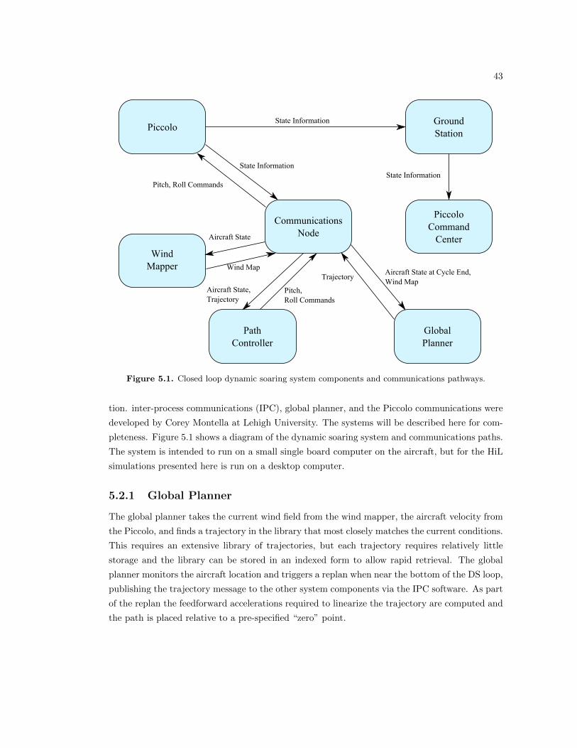
43
Communications
Node
Wind
Mapper
Path
Controller
Global
Planner
PiccoloGround
Station
Piccolo
Command
Center
State Information
Pitch, Roll Commands
Aircraft State at Cycle End,
Wind MapTrajectory
Wind Map
Aircraft State
Pitch,
Roll Commands
Aircraft State,
Trajectory
State Information
State Information
Figure 5.1. Closed loop dynamic soaring system components and communications pathways.
tion. inter-process communications (IPC), global planner, and the Piccolo communications were
developed by Corey Montella at Lehigh University. The systems will be described here for com-
pleteness. Figure 5.1 shows a diagram of the dynamic soaring system and communications paths.
The system is intended to run on a small single board computer on the aircraft, but for the HiL
simulations presented here is run on a desktop computer.
5.2.1 Global Planner
The global planner takes the current wind field from the wind mapper, the aircraft velocity from
the Piccolo, and finds a trajectory in the library that most closely matches the current conditions.
This requires an extensive library of trajectories, but each trajectory requires relatively little
storage and the library can be stored in an indexed form to allow rapid retrieval. The global
planner monitors the aircraft location and triggers a replan when near the bottom of the DS loop,
publishing the trajectory message to the other system components via the IPC software. As part
of the replan the feedforward accelerations required to linearize the trajectory are computed and
the path is placed relative to a pre-specified “zero” point.
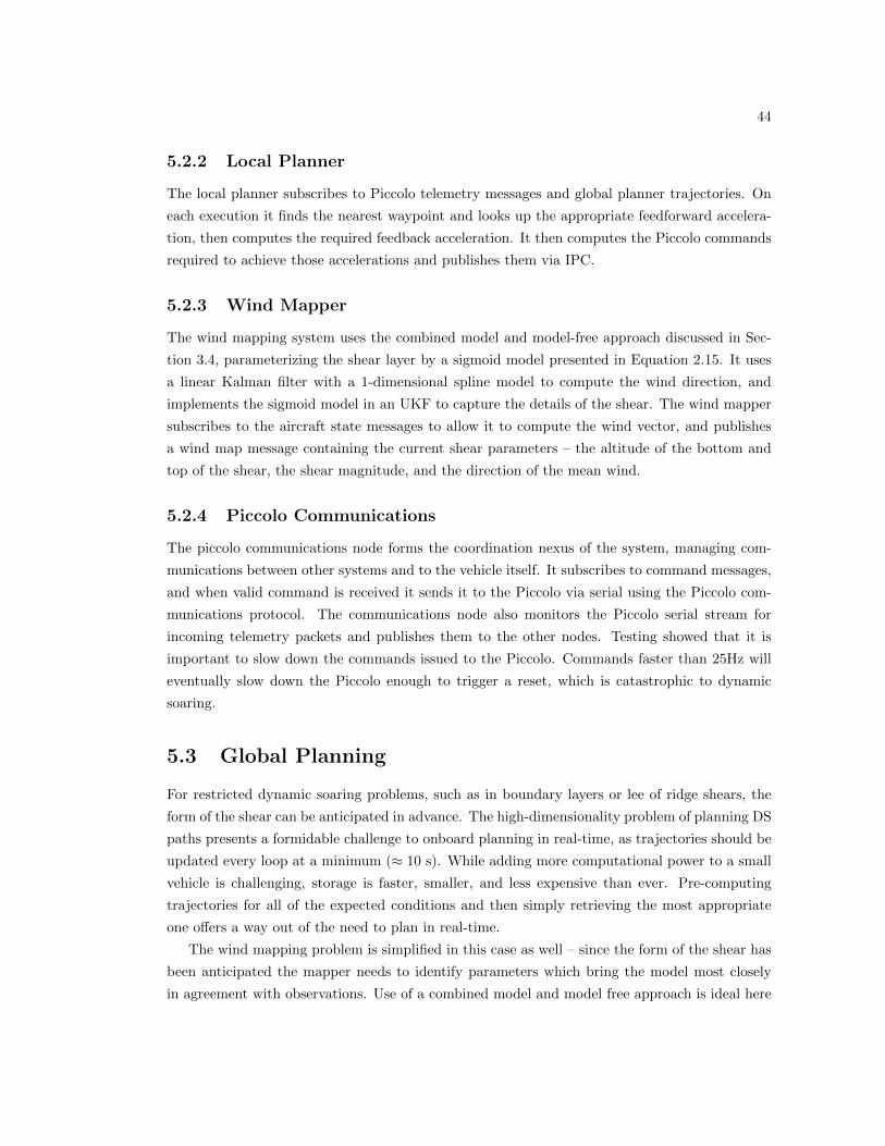
44
5.2.2 Local Planner
The local planner subscribes to Piccolo telemetry messages and global planner trajectories. On
each execution it finds the nearest waypoint and looks up the appropriate feedforward accelera-
tion, then computes the required feedback acceleration. It then computes the Piccolo commands
required to achieve those accelerations and publishes them via IPC.
5.2.3 Wind Mapper
The wind mapping system uses the combined model and model-free approach discussed in Sec-
tion 3.4, parameterizing the shear layer by a sigmoid model presented in Equation 2.15. It uses
a linear Kalman filter with a 1-dimensional spline model to compute the wind direction, and
implements the sigmoid model in an UKF to capture the details of the shear. The wind mapper
subscribes to the aircraft state messages to allow it to compute the wind vector, and publishes
a wind map message containing the current shear parameters – the altitude of the bottom and
top of the shear, the shear magnitude, and the direction of the mean wind.
5.2.4 Piccolo Communications
The piccolo communications node forms the coordination nexus of the system, managing com-
munications between other systems and to the vehicle itself. It subscribes to command messages,
and when valid command is received it sends it to the Piccolo via serial using the Piccolo com-
munications protocol. The communications node also monitors the Piccolo serial stream for
incoming telemetry packets and publishes them to the other nodes. Testing showed that it is
important to slow down the commands issued to the Piccolo. Commands faster than 25Hz will
eventually slow down the Piccolo enough to trigger a reset, which is catastrophic to dynamic
soaring.
5.3 Global Planning
For restricted dynamic soaring problems, such as in boundary layers or lee of ridge shears, the
form of the shear can be anticipated in advance. The high-dimensionality problem of planning DS
paths presents a formidable challenge to onboard planning in real-time, as trajectories should be
updated every loop at a minimum (≈ 10 s). While adding more computational power to a small
vehicle is challenging, storage is faster, smaller, and less expensive than ever. Pre-computing
trajectories for all of the expected conditions and then simply retrieving the most appropriate
one offers a way out of the need to plan in real-time.
The wind mapping problem is simplified in this case as well – since the form of the shear has
been anticipated the mapper needs to identify parameters which bring the model most closely
in agreement with observations. Use of a combined model and model free approach is ideal here
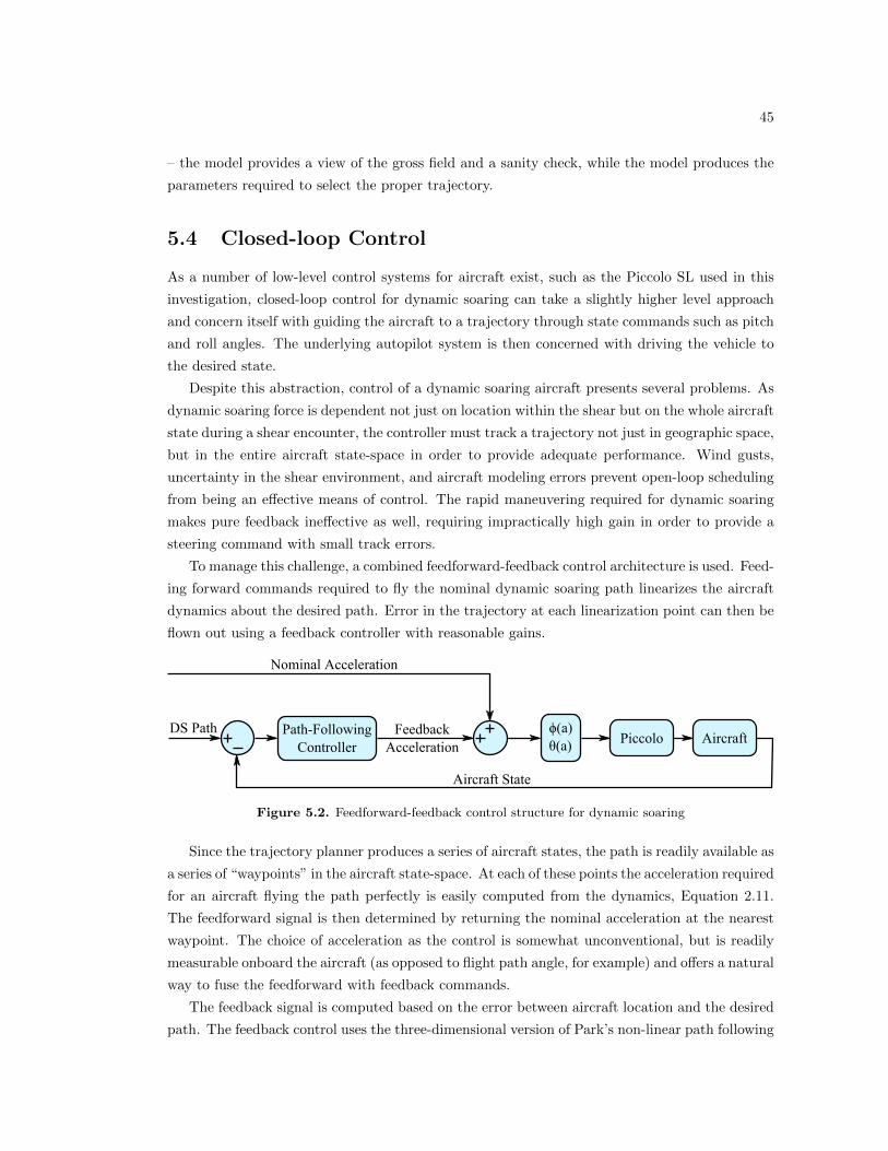
45
– the model provides a view of the gross field and a sanity check, while the model produces the
parameters required to select the proper trajectory.
5.4 Closed-loop Control
As a number of low-level control systems for aircraft exist, such as the Piccolo SL used in this
investigation, closed-loop control for dynamic soaring can take a slightly higher level approach
and concern itself with guiding the aircraft to a trajectory through state commands such as pitch
and roll angles. The underlying autopilot system is then concerned with driving the vehicle to
the desired state.
Despite this abstraction, control of a dynamic soaring aircraft presents several problems. As
dynamic soaring force is dependent not just on location within the shear but on the whole aircraft
state during a shear encounter, the controller must track a trajectory not just in geographic space,
but in the entire aircraft state-space in order to provide adequate performance. Wind gusts,
uncertainty in the shear environment, and aircraft modeling errors prevent open-loop scheduling
from being an effective means of control. The rapid maneuvering required for dynamic soaring
makes pure feedback ineffective as well, requiring impractically high gain in order to provide a
steering command with small track errors.
To manage this challenge, a combined feedforward-feedback control architecture is used. Feed-
ing forward commands required to fly the nominal dynamic soaring path linearizes the aircraft
dynamics about the desired path. Error in the trajectory at each linearization point can then be
flown out using a feedback controller with reasonable gains.
Path-Following
Controller
DS Path
Nominal Acceleration
ϕ(a)
θ(a)Piccolo Aircraft
Aircraft State
Feedback
Acceleration
Figure 5.2. Feedforward-feedback control structure for dynamic soaring
Since the trajectory planner produces a series of aircraft states, the path is readily available as
a series of “waypoints” in the aircraft state-space. At each of these points the acceleration required
for an aircraft flying the path perfectly is easily computed from the dynamics, Equation 2.11.
The feedforward signal is then determined by returning the nominal acceleration at the nearest
waypoint. The choice of acceleration as the control is somewhat unconventional, but is readily
measurable onboard the aircraft (as opposed to flight path angle, for example) and offers a natural
way to fuse the feedforward with feedback commands.
The feedback signal is computed based on the error between aircraft location and the desired
path. The feedback control uses the three-dimensional version of Park’s non-linear path following
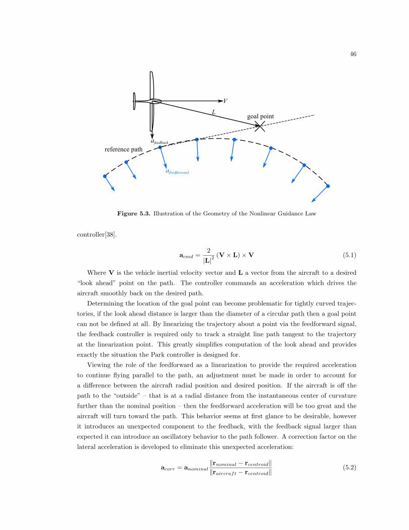
46
L
V
afeedbackreference path
goal point
afeedforward
Figure 5.3. Illustration of the Geometry of the Nonlinear Guidance Law
controller[38].
acmd =2
|L|2(V × L)×V (5.1)
Where V is the vehicle inertial velocity vector and L a vector from the aircraft to a desired
“look ahead” point on the path. The controller commands an acceleration which drives the
aircraft smoothly back on the desired path.
Determining the location of the goal point can become problematic for tightly curved trajec-
tories, if the look ahead distance is larger than the diameter of a circular path then a goal point
can not be defined at all. By linearizing the trajectory about a point via the feedforward signal,
the feedback controller is required only to track a straight line path tangent to the trajectory
at the linearization point. This greatly simplifies computation of the look ahead and provides
exactly the situation the Park controller is designed for.
Viewing the role of the feedforward as a linearization to provide the required acceleration
to continue flying parallel to the path, an adjustment must be made in order to account for
a difference between the aircraft radial position and desired position. If the aircraft is off the
path to the “outside” – that is at a radial distance from the instantaneous center of curvature
further than the nominal position – then the feedforward acceleration will be too great and the
aircraft will turn toward the path. This behavior seems at first glance to be desirable, however
it introduces an unexpected component to the feedback, with the feedback signal larger than
expected it can introduce an oscillatory behavior to the path follower. A correction factor on the
lateral acceleration is developed to eliminate this unexpected acceleration:
acorr = anominal‖rnominal − rcentroid‖‖raircraft − rcentroid‖
(5.2)
47
5.5 DS Control with the Piccolo Autopilot
Since both controllers yield acceleration commands in inertial axes, they can be easily combined
by simply summing into a total acceleration command. While making command composition
simple, this still presents a difficulty as the lowest-level commands that the Piccolo will accept
are Euler angle commands. Translating acceleration commands into a form actionable by the
Piccolo is accomplished through the following process:
First, the commanded accelerations must be rotated by the heading angle into a coordinate
frame with x in the direction of the flight path. Making the assumption that γ = θ, desired pitch
rates can then be determined through kinematics:
θ =−azVa
(5.3)
Observing that the lateral acceleration must come from the tilted lift vector of the banked
wing, the required lateral acceleration can be expressed:
ay = (az + g) tanφ (5.4)
Which can be easily rearranged to give a bank angle which will provide the proper y to z
acceleration ratio.
φ = tan−1(ay, az + g) (5.5)
The achieved y acceleration will then be as commanded provided that the required z axis
acceleration is achieved. Referring to the relationship between acceleration and aircraft kine-
matics detailed in equation 5.3, the required z acceleration can be achieved through appropriate
θ. Unfortunately, θ cannot be directly commanded to the Piccolo. The autopilot will however,
attempt to achieve a first-order response to pitch angle commands. The time constant is known
as it is a specified autopilot configuration parameter, so a pitch step command can be constructed
to achieve the desired pitch rate.
θcmd =1
Tθθcmd + θ (5.6)
As a practical consideration, it is important to note that there is no guarantee that the
solution provided will be a feasible one for the autopilot to fly – for example, a sufficiently strong
downward acceleration may require the aircraft to roll inverted, however the Piccolo autopilot
will not allow roll angles greater than 90◦. This limitation makes it critical that the trajectory
generated is not only feasible for the aircraft to fly, but is not at the limits of autopilot capability
in order to ensure sufficient maneuvering margin exists to fly out trajectory errors.
Another practical consideration in the implementation of this path following controller is
selection of the look-ahead distance, L. This serves as a sort of convergence tuning parameter for
the controller – smaller values of L lead to more rapid correction of flight path error, but can also
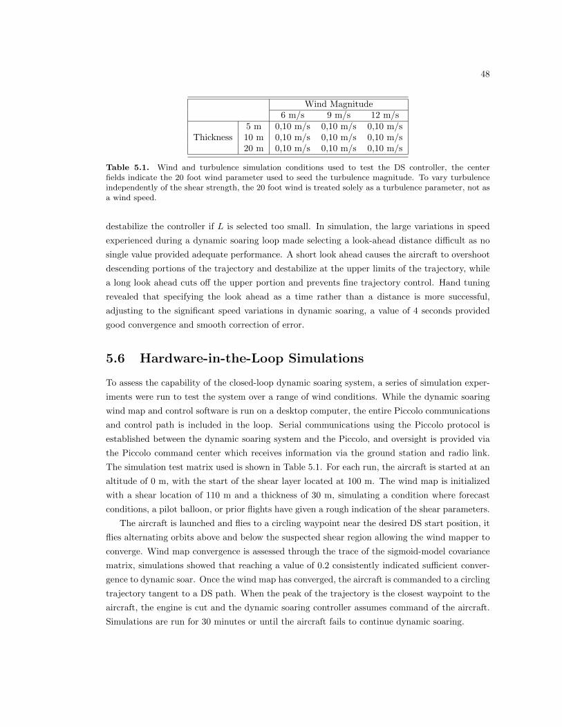
48
Wind Magnitude6 m/s 9 m/s 12 m/s
5 m 0,10 m/s 0,10 m/s 0,10 m/sThickness 10 m 0,10 m/s 0,10 m/s 0,10 m/s
20 m 0,10 m/s 0,10 m/s 0,10 m/s
Table 5.1. Wind and turbulence simulation conditions used to test the DS controller, the centerfields indicate the 20 foot wind parameter used to seed the turbulence magnitude. To vary turbulenceindependently of the shear strength, the 20 foot wind is treated solely as a turbulence parameter, not asa wind speed.
destabilize the controller if L is selected too small. In simulation, the large variations in speed
experienced during a dynamic soaring loop made selecting a look-ahead distance difficult as no
single value provided adequate performance. A short look ahead causes the aircraft to overshoot
descending portions of the trajectory and destabilize at the upper limits of the trajectory, while
a long look ahead cuts off the upper portion and prevents fine trajectory control. Hand tuning
revealed that specifying the look ahead as a time rather than a distance is more successful,
adjusting to the significant speed variations in dynamic soaring, a value of 4 seconds provided
good convergence and smooth correction of error.
5.6 Hardware-in-the-Loop Simulations
To assess the capability of the closed-loop dynamic soaring system, a series of simulation exper-
iments were run to test the system over a range of wind conditions. While the dynamic soaring
wind map and control software is run on a desktop computer, the entire Piccolo communications
and control path is included in the loop. Serial communications using the Piccolo protocol is
established between the dynamic soaring system and the Piccolo, and oversight is provided via
the Piccolo command center which receives information via the ground station and radio link.
The simulation test matrix used is shown in Table 5.1. For each run, the aircraft is started at an
altitude of 0 m, with the start of the shear layer located at 100 m. The wind map is initialized
with a shear location of 110 m and a thickness of 30 m, simulating a condition where forecast
conditions, a pilot balloon, or prior flights have given a rough indication of the shear parameters.
The aircraft is launched and flies to a circling waypoint near the desired DS start position, it
flies alternating orbits above and below the suspected shear region allowing the wind mapper to
converge. Wind map convergence is assessed through the trace of the sigmoid-model covariance
matrix, simulations showed that reaching a value of 0.2 consistently indicated sufficient conver-
gence to dynamic soar. Once the wind map has converged, the aircraft is commanded to a circling
trajectory tangent to a DS path. When the peak of the trajectory is the closest waypoint to the
aircraft, the engine is cut and the dynamic soaring controller assumes command of the aircraft.
Simulations are run for 30 minutes or until the aircraft fails to continue dynamic soaring.
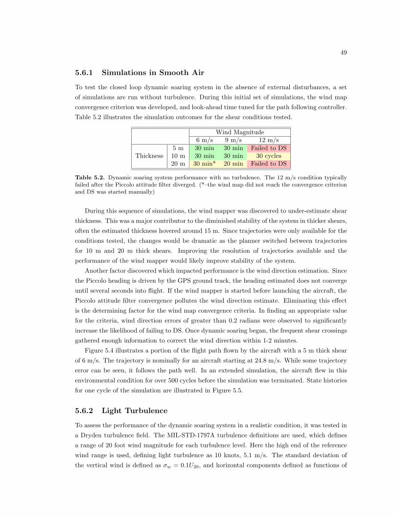
49
5.6.1 Simulations in Smooth Air
To test the closed loop dynamic soaring system in the absence of external disturbances, a set
of simulations are run without turbulence. During this initial set of simulations, the wind map
convergence criterion was developed, and look-ahead time tuned for the path following controller.
Table 5.2 illustrates the simulation outcomes for the shear conditions tested.
Wind Magnitude6 m/s 9 m/s 12 m/s
5 m 30 min 30 min Failed to DSThickness 10 m 30 min 30 min 30 cycles
20 m 30 min* 20 min Failed to DS
Table 5.2. Dynamic soaring system performance with no turbulence. The 12 m/s condition typicallyfailed after the Piccolo attitude filter diverged. (*–the wind map did not reach the convergence criterionand DS was started manually)
During this sequence of simulations, the wind mapper was discovered to under-estimate shear
thickness. This was a major contributor to the diminished stability of the system in thicker shears,
often the estimated thickness hovered around 15 m. Since trajectories were only available for the
conditions tested, the changes would be dramatic as the planner switched between trajectories
for 10 m and 20 m thick shears. Improving the resolution of trajectories available and the
performance of the wind mapper would likely improve stability of the system.
Another factor discovered which impacted performance is the wind direction estimation. Since
the Piccolo heading is driven by the GPS ground track, the heading estimated does not converge
until several seconds into flight. If the wind mapper is started before launching the aircraft, the
Piccolo attitude filter convergence pollutes the wind direction estimate. Eliminating this effect
is the determining factor for the wind map convergence criteria. In finding an appropriate value
for the criteria, wind direction errors of greater than 0.2 radians were observed to significantly
increase the likelihood of failing to DS. Once dynamic soaring began, the frequent shear crossings
gathered enough information to correct the wind direction within 1-2 minutes.
Figure 5.4 illustrates a portion of the flight path flown by the aircraft with a 5 m thick shear
of 6 m/s. The trajectory is nominally for an aircraft starting at 24.8 m/s. While some trajectory
error can be seen, it follows the path well. In an extended simulation, the aircraft flew in this
environmental condition for over 500 cycles before the simulation was terminated. State histories
for one cycle of the simulation are illustrated in Figure 5.5.
5.6.2 Light Turbulence
To assess the performance of the dynamic soaring system in a realistic condition, it was tested in
a Dryden turbulence field. The MIL-STD-1797A turbulence definitions are used, which defines
a range of 20 foot wind magnitude for each turbulence level. Here the high end of the reference
wind range is used, defining light turbulence as 10 knots, 5.1 m/s. The standard deviation of
the vertical wind is defined as σw = 0.1U20, and horizontal components defined as functions of
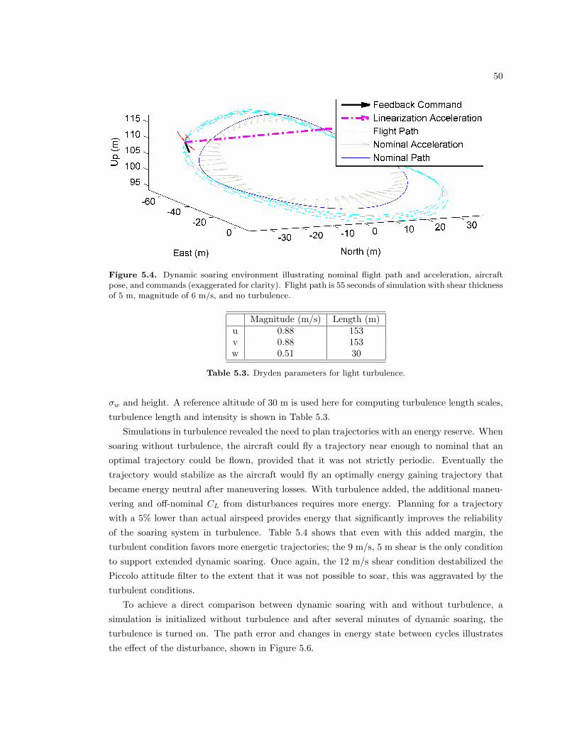
50
Figure 5.4. Dynamic soaring environment illustrating nominal flight path and acceleration, aircraftpose, and commands (exaggerated for clarity). Flight path is 55 seconds of simulation with shear thicknessof 5 m, magnitude of 6 m/s, and no turbulence.
Magnitude (m/s) Length (m)u 0.88 153v 0.88 153w 0.51 30
Table 5.3. Dryden parameters for light turbulence.
σw and height. A reference altitude of 30 m is used here for computing turbulence length scales,
turbulence length and intensity is shown in Table 5.3.
Simulations in turbulence revealed the need to plan trajectories with an energy reserve. When
soaring without turbulence, the aircraft could fly a trajectory near enough to nominal that an
optimal trajectory could be flown, provided that it was not strictly periodic. Eventually the
trajectory would stabilize as the aircraft would fly an optimally energy gaining trajectory that
became energy neutral after maneuvering losses. With turbulence added, the additional maneu-
vering and off-nominal CL from disturbances requires more energy. Planning for a trajectory
with a 5% lower than actual airspeed provides energy that significantly improves the reliability
of the soaring system in turbulence. Table 5.4 shows that even with this added margin, the
turbulent condition favors more energetic trajectories; the 9 m/s, 5 m shear is the only condition
to support extended dynamic soaring. Once again, the 12 m/s shear condition destabilized the
Piccolo attitude filter to the extent that it was not possible to soar, this was aggravated by the
turbulent conditions.
To achieve a direct comparison between dynamic soaring with and without turbulence, a
simulation is initialized without turbulence and after several minutes of dynamic soaring, the
turbulence is turned on. The path error and changes in energy state between cycles illustrates
the effect of the disturbance, shown in Figure 5.6.
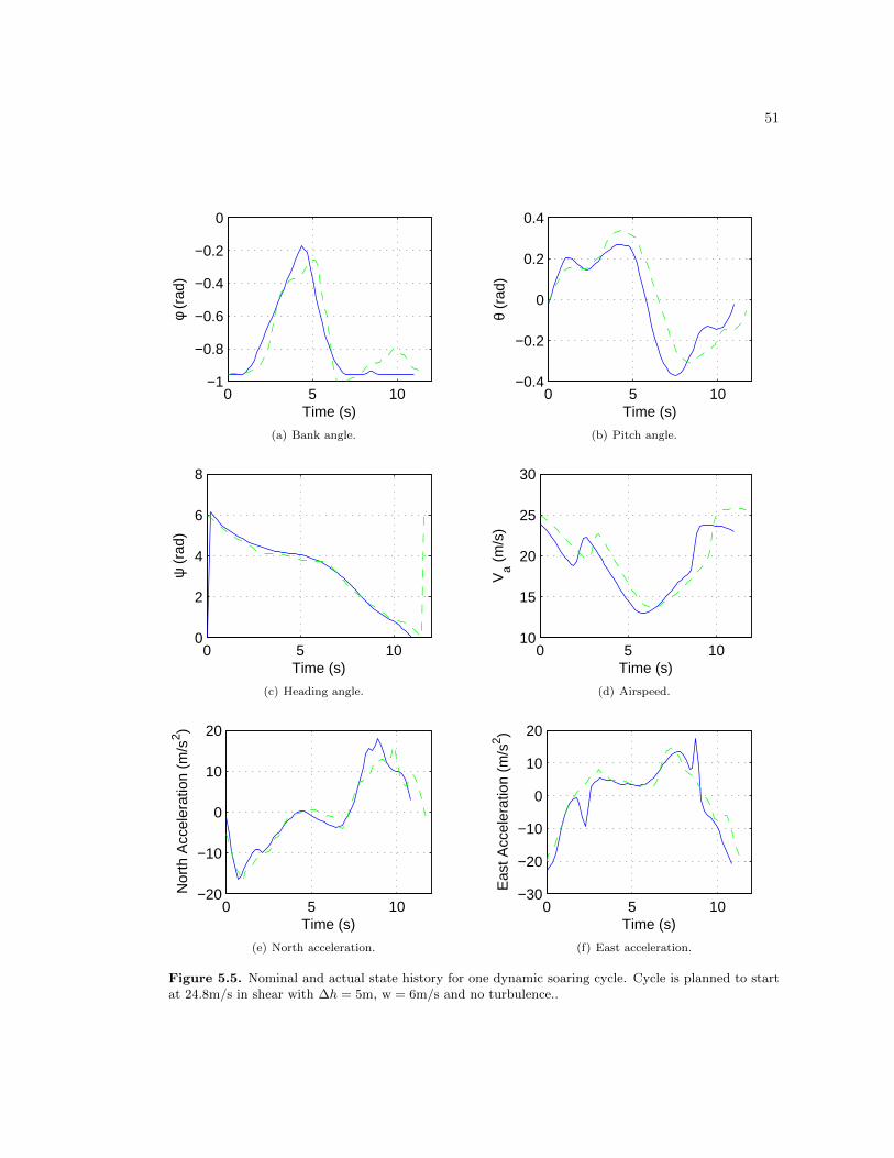
51
0 5 10−1
−0.8
−0.6
−0.4
−0.2
0
Time (s)
φ (r
ad)
(a) Bank angle.
0 5 10−0.4
−0.2
0
0.2
0.4
Time (s)
θ (r
ad)
(b) Pitch angle.
0 5 100
2
4
6
8
Time (s)
ψ (
rad)
(c) Heading angle.
0 5 1010
15
20
25
30
Time (s)
Va (
m/s
)
(d) Airspeed.
0 5 10−20
−10
0
10
20
Time (s)
Nor
th A
ccel
erat
ion
(m/s
2 )
(e) North acceleration.
0 5 10−30
−20
−10
0
10
20
Time (s)
Eas
t Acc
eler
atio
n (m
/s2 )
(f) East acceleration.
Figure 5.5. Nominal and actual state history for one dynamic soaring cycle. Cycle is planned to startat 24.8m/s in shear with ∆h = 5m, w = 6m/s and no turbulence..
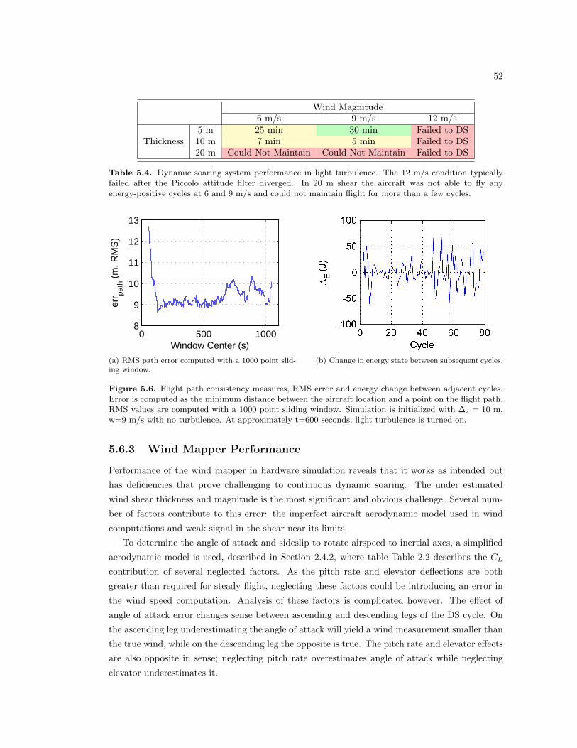
52
Wind Magnitude6 m/s 9 m/s 12 m/s
5 m 25 min 30 min Failed to DSThickness 10 m 7 min 5 min Failed to DS
20 m Could Not Maintain Could Not Maintain Failed to DS
Table 5.4. Dynamic soaring system performance in light turbulence. The 12 m/s condition typicallyfailed after the Piccolo attitude filter diverged. In 20 m shear the aircraft was not able to fly anyenergy-positive cycles at 6 and 9 m/s and could not maintain flight for more than a few cycles.
0 500 10008
9
10
11
12
13
Window Center (s)
err pa
th (
m, R
MS
)
(a) RMS path error computed with a 1000 point slid-ing window.
(b) Change in energy state between subsequent cycles.
Figure 5.6. Flight path consistency measures, RMS error and energy change between adjacent cycles.Error is computed as the minimum distance between the aircraft location and a point on the flight path,RMS values are computed with a 1000 point sliding window. Simulation is initialized with ∆z = 10 m,w=9 m/s with no turbulence. At approximately t=600 seconds, light turbulence is turned on.
5.6.3 Wind Mapper Performance
Performance of the wind mapper in hardware simulation reveals that it works as intended but
has deficiencies that prove challenging to continuous dynamic soaring. The under estimated
wind shear thickness and magnitude is the most significant and obvious challenge. Several num-
ber of factors contribute to this error: the imperfect aircraft aerodynamic model used in wind
computations and weak signal in the shear near its limits.
To determine the angle of attack and sideslip to rotate airspeed to inertial axes, a simplified
aerodynamic model is used, described in Section 2.4.2, where table Table 2.2 describes the CL
contribution of several neglected factors. As the pitch rate and elevator deflections are both
greater than required for steady flight, neglecting these factors could be introducing an error in
the wind speed computation. Analysis of these factors is complicated however. The effect of
angle of attack error changes sense between ascending and descending legs of the DS cycle. On
the ascending leg underestimating the angle of attack will yield a wind measurement smaller than
the true wind, while on the descending leg the opposite is true. The pitch rate and elevator effects
are also opposite in sense; neglecting pitch rate overestimates angle of attack while neglecting
elevator underestimates it.
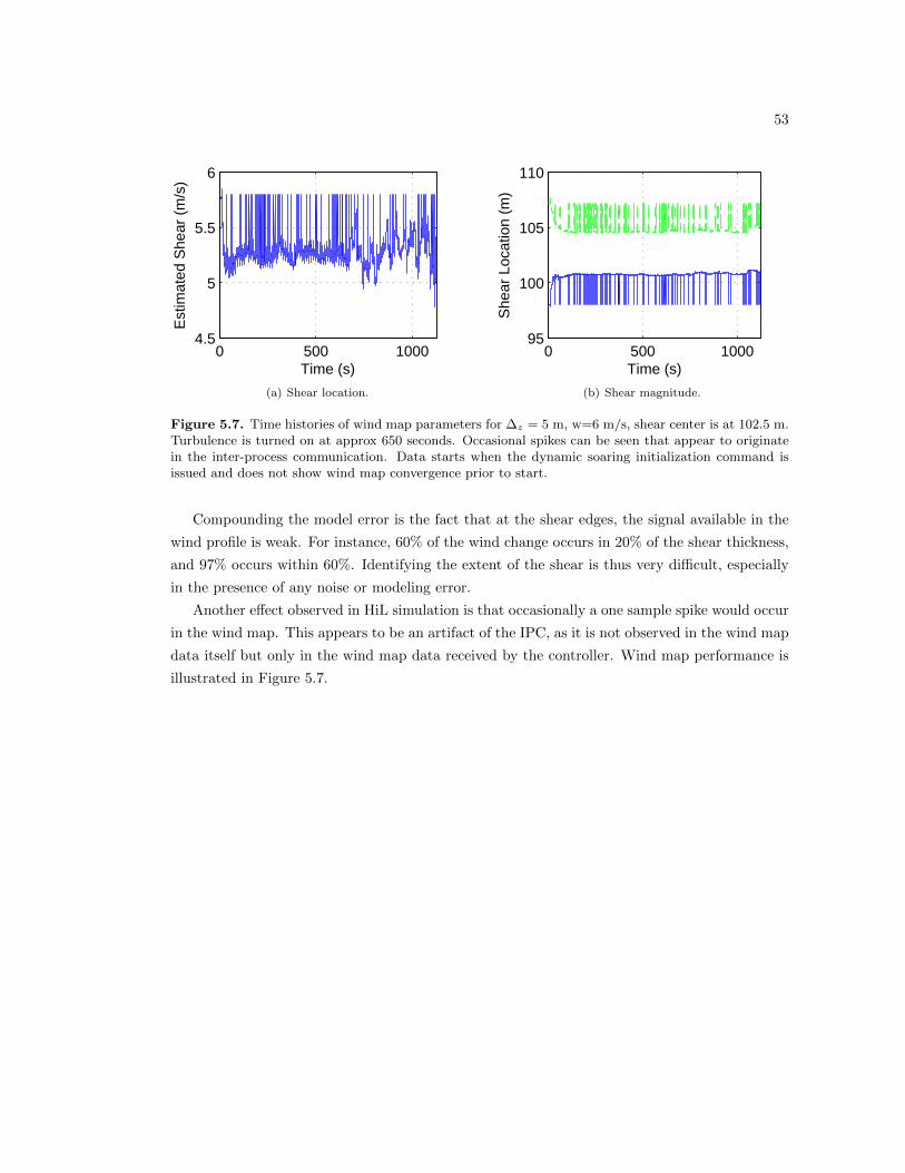
53
0 500 10004.5
5
5.5
6
Time (s)
Est
imat
ed S
hear
(m
/s)
(a) Shear location.
0 500 100095
100
105
110
Time (s)
She
ar L
ocat
ion
(m)
(b) Shear magnitude.
Figure 5.7. Time histories of wind map parameters for ∆z = 5 m, w=6 m/s, shear center is at 102.5 m.Turbulence is turned on at approx 650 seconds. Occasional spikes can be seen that appear to originatein the inter-process communication. Data starts when the dynamic soaring initialization command isissued and does not show wind map convergence prior to start.
Compounding the model error is the fact that at the shear edges, the signal available in the
wind profile is weak. For instance, 60% of the wind change occurs in 20% of the shear thickness,
and 97% occurs within 60%. Identifying the extent of the shear is thus very difficult, especially
in the presence of any noise or modeling error.
Another effect observed in HiL simulation is that occasionally a one sample spike would occur
in the wind map. This appears to be an artifact of the IPC, as it is not observed in the wind map
data itself but only in the wind map data received by the controller. Wind map performance is
illustrated in Figure 5.7.
Chapter 6Conclusions
Endurance and range continues to challenge small uas, especially in cost-sensitive applications.
Birds of similar mass and size realize dramatically superior range and endurance by harvesting
energy from vertical velocities and shear in the atmosphere, indicating a means to improve the
performance of small uas. While energy harvesting has been demonstrated for some environ-
mental conditions, uas still lack the ability to map their atmospheric surroundings in support of
energy harvesting.
A means to map the wind field and shear environment has been presented as an enabling
technology to harvesting energy from the atmosphere for small uas. Techniques are developed
to map both known and arbitrary environments and to harvest energy from those environments,
closing a loop around the energy harvesting problem from environmental mapping to exploitation.
6.1 Use of Wind Maps in Energy Harvesting
6.1.1 Static Soaring
A technique to map arbitrary updraft structures using basis splines is developed. The technique
is demonstrated in simulated encounters with convective updrafts, building a map which captures
important features of the wind field. A technique to exploit this map is developed and demon-
strates performance similar to existing thermalling techniques, and shows resilience to updraft
structure and size. An existing path following controller is adapted to the purpose of thermal
exploitation, providing the capability to track complex paths through a thermal.
6.1.2 Dynamic Soaring
The wind mapping technique is also applied to dynamic soaring. Using an a priori model
structure, the mapper estimates features of the shears in lee of ridge environments. This enables
selection of an appropriate trajectory for dynamic soaring. The mapper is able to reject turbulent
55
disturbances and track the shear during dynamic soaring, though the rapid shear crossings and
imperfect aircraft model degrades estimates.
A feedback linearization control architecture is developed for dynamic soaring which uses
feedforward accelerations to linearize the trajectory and a feedback controller to fly out path
errors. The controller is demonstrated to provide trajectory tracking adequate to enable dynamic
soaring in several shear environments, though the use of optimal trajectory planning is shown
to be problematic, especially for flight in turbulence.. HiL simulations show a COTS autopilot
capable of dynamic soaring.
6.2 Recommendations for Future Work
6.2.1 Static Soaring and Wind Maps
Incorporating models for the time evolution of updrafts, such as diffusion-advection equations
should be investigated. This could enable the wind map to explicitly model the drift and expan-
sion of thermals through their lifetime, eliminating a source of uncertainty in thermal exploitation.
More advanced thermal exploitation algorithms should also be developed which can plan trajec-
tories that for instance, sacrifice climb rate during one portion of a cycle to fly through areas of
very strong lift.
In-flight experiments of thermal modeling are also critical to establish that this capability
works in the uncertain and complex environment of real thermals, few of which in the author’s
experience, are shaped quite like engineering models. Investigation in the application of thermal
modeling techniques to cockpit displays for human pilots is also warranted.
6.2.2 Closed-Loop Dynamic Soaring
Autonomous dynamic soaring remains a challenging and relatively unexplored field, a number of
challenges that warrant further research were noted in this work.
The Piccolo state estimation filter presents several challenges to dynamic soaring. The large
accelerations, rapid turns and altitude changes, and wide speed variation can destabilize the
attitude filter. This effect is exacerbated in conditions of strong wind shear (introducing greater
disturbances at shear crossing) and turbulence. Attitude filter divergence was found to limit
soarable conditions in the more extreme cases. Future DS systems should have state estimation
solutions developed with a focus on reliability during acceleration and large disturbances.
Another challenge the attitude filter posed was in heading bias. Since the heading is derived
from GPS track, it is susceptible to errors introduced by wind. Ordinarily these errors would be
eliminated as the aircraft turns: the wind components become observable when the aircraft track
changes and the heading can be determined. While dynamic soaring however, the wind changes
within a single circle. Since the aircraft only turns a single direction, this problem is exacerbated.
In order to obtain reliable estimates of the wind direction it was necessary to include a heuristic
factor accounting for this discrepancy, a value of 0.06 radians was found to yield satisfactory
56
results. Future solutions should include a magnetometer or other external heading reference
system.
Computing controls that the Piccolo accepts is another source of trajectory error. The lon-
gitudinal control especially poses a challenge. Since the Piccolo doesn’t perfectly achieve a first
order response, the longitudinal tracking has error that often caused the aircraft to overshoot
the trajectory low point by up to 4-5 meters. Depending on the terrain surrounding a ridge,
this is potentially a tolerable error. When considering boundary layer soaring however, providing
sufficient safety margin would make soaring impossible. An operation dynamic soaring system
will likely need an autopilot developed for the purpose and providing low-level commands.
Beyond challenges directly posed by the Piccolo, the nature of the paths generated poses
a challenge. Computing optimal trajectories is an interesting academic exercise, and provides
useful bounds on the potential of dynamic soaring, but optimal paths are not operational ones.
In the presence of control errors or turbulence, the aircraft state will not match the optimal
state. Energy extraction is then decreased relative to the nominal trajectory and the aircraft
will “fall off” the dynamic soaring cycle. Here the problem was handled by planning paths to
maximize extraction and selecting a new path at the bottom of each cycle. In this sense, the
trajectories were not fully closed in the aircraft state-space, but since they close in geometric
space, continuous flight is possible. This approach however, does not always provide enough
energy for the aircraft to satisfactorily complete the chosen cycle until the next replan, so paths
were selected with a 5% lower initial speed that the aircraft’s actual speed. Robust trajectory
planning, such as that explored by Flanzer[30] should be investigated in HiL simulation.
Wind estimation during dynamic soaring is another difficulty. Before dynamic soaring, the
aircraft can slowly traverse the shear layer to gather information about the structure and width
of the shear. During dynamic soaring however, the strongest shear is traversed as rapidly as
possible to maximize energy exploitation. The wind mapper is thus modeling with very little
information. In simulation, the rapid shear crossing is observed to cause the wind mapper to
underestimate the thickness and strength of a shear layer. As these two factors have the opposite
effect on energy extracted, the impact on the aircraft is somewhat reduced. The underestimated
shear thickness the primary challenge, a heuristic adjustment was used in this work, increasing
the thickness by 10%. Further research into the cause of this error is needed, and a trajectory
database with higher resolution in environmental conditions should be employed to minimize the
effect of mapping errors.
Bibliography
[1] U.S. Department of Transportation, F. A. A. (2013) Glider Flying Handbook, Okla-homa City.
[2] (2010) FOX Assembly Instructions, Tech. rep., EScale.
[3] Van der Hoven, I. (1957) “Power Spectrum of Horizontal Wind Speed in the FrequencyRange from 0.0007 to 900 Cycles per Hour,” Journal of Meteorology, 14.
[4] Jones, G. P. I., L. G. Pearsltine, and F. H. Percival (2006) “An assessment of smallunmanned aerial vehicles for wildlife research,” Wildlife Society . . . , 34(3).
[5] Bailey, P. (2013), “Remote-controlled helicopter tested for use in vineyard applications,”.URL http://www.caes.ucdavis.edu/news/articles/2013/06/
remote-controlled-helicopter-tested-for-use-in-vineyard-applications
[6] Lin, P.-H. (2006) “OBSERVATIONS: The First Successful Typhoon Eyewall-PenetrationReconnaissance Flight Mission Conducted by the Unmanned Aerial Vehicle, Aerosonde,”Bulletin of the American Meteorological Society, 87(11), pp. 1481–1483.
[7] Elston, J. and J. Roadman (2011) “The tempest unmanned aircraft system for in situobservations of tornadic supercells: design and VORTEX2 flight results,” Journal of Field. . . , 28(4), pp. 461–483.
[8] Garamone, J. (2005), “ScanEagle Proves Worth in Fallujah Fight,” .URL http://www.defense.gov/News/NewsArticle.aspx?ID=24397
[9] Pennycuick, C. (1982) “The flight of petrels and albatrosses (Procellariiformes), observedin South Georgia and its vicinity,” Philosophical Transactions of the . . . , 300(1098), pp.75–106.
[10] Sachs, G., J. Traugott, and A. Nesterova (2012) “Flying at No Mechanical EnergyCost: Disclosing the Secret of Wandering Albatrosses,” PloS one, 7(9).
[11] Shannon, H. D., G. S. Young, M. A. Yates, M. R. Fuller, and S. Seegar (2002)“American White Pelican Soaring Flight Times and Altitudes Relative to Changes in Ther-mal Depth and Intensity,” The Condor, 104(3), pp. 679–683.
[12] Klaassen, M. (1996) “Metabolic constraints on long-distance migration in birds,” TheJournal of experimental biology, 199(Pt 1), pp. 57–64.
58
[13] Allen, M. (2005) “Autonomous Soaring for Improved Endurance of a Small UninhabitedAir Vehicle,” Proceedings of the 43rd Aerospace Sciences Meeting, . . . , pp. 1–13.
[14] ——— (2007) Guidance and control for an autonomous soaring UAV, Tech. Rep. April,NASA Dryden Flight Research Center.
[15] Edwards, D. J. and L. M. Silberberg (2010) “Autonomous Soaring: The MontagueCross-Country Challenge,” Journal of Aircraft, 47(5), pp. 1763–1769.
[16] Reichmann, H. (1981) Cross-Country Soaring.
[17] Drake, V. and R. Farrow (1988) “The Influence of Atmospheric Structure and Motionson Insect Migration,” Annual Review of Entomology, 33, pp. 183–210.
[18] Rayleigh, L. (1883) “The Soaring of Birds,” Nature, 27(701), pp. 534–535.
[19] Andersson, K., I. Kaminer, V. Dobrokhodov, and V. Cichella (2012) “ThermalCentering Control for Autonomous Soaring; Stability Analysis and Flight Test Results,”Journal of Guidance, Control, and Dynamics, 35(3), pp. 963–975.
[20] MacCready, P. B. J. (1958) “Optimum Airspeed Selector,” Soaring, (1), pp. 10–11.
[21] Grubisic, V. and B. J. Billings (2008) “Climatology of the Sierra Nevada Mountain-WaveEvents,” Monthly Weather Review, 136(2), pp. 757–768.
[22] Nielsen, J. W. (1992) “In Situ Observations of Kelvin-Helmholtz Waves along a FrontalInversion,” Journal of the Atmospheric Sciences, 49(5), pp. 369–386.
[23] Chakrabarty, A. and J. W. Langelaan (2011) “Energy-Based Long-Range Path Plan-ning for Soaring-Capable Unmanned Aerial Vehicles,” Journal of Guidance, Control, andDynamics, 34(4), pp. 1002–1015.
[24] Klemperer, W. (1958) “A Review on the Theory of Dynamic Soaring,” Technical Soaring.
[25] Wood, C. (1973) “The flight of albatrosses (a computer simulation),” Ibis, pp. 244–256.
[26] (2013), “RC Speeds: Fastest 20 Aircraft,” .URL http://rcspeeds.com/aircraft.aspx?AirplaneType=BD
[27] Sachs, G. and O. da Costa (2006) “Dynamic soaring in altitude region below jet streams,”AIAA Guidance, Navigation, and Control Conference, (August), pp. 1–11.
[28] Grenestedt, J. L. and J. R. Spletzer (2010) “Towards Perpetual Flight of a GlidingUnmanned Aerial Vehicle in the Jet Stream,” IEEE Conference on Decision and Control.
[29] Sukumar, P. and M. Selig (2010) “Dynamic Soaring of Sailplanes over Open Fields,”(July).
[30] Flanzer, T. C., G. C. Bower, and I. M. Kroo (2012) “Robust Trajectory Optimizationfor Dynamic Soaring,” AIAA Guidance, Navigation, and Control Conference, (August), pp.1–22.
[31] Sachs, G. (2005) “Minimum shear wind strength required for dynamic soaring of alba-trosses,” Ibis, 147, pp. 1–10.
[32] Zhao, Y. J. (2004) “Optimal patterns of glider dynamic soaring,” Optimal Control Appli-cations and Methods, 25(2), pp. 67–89.
59
[33] Zhao, Y. J. and Y. C. Qi (2004) “Minimum fuel powered dynamic soaring of unmannedaerial vehicles utilizing wind gradients,” Optimal Control Applications and Methods, 25(5),pp. 211–233.
[34] Deittert, M., A. Richards, C. a. Toomer, and A. Pipe (2009) “Engineless UnmannedAerial Vehicle Propulsion by Dynamic Soaring,” Journal of Guidance, Control, and Dynam-ics, 32(5), pp. 1446–1457.
[35] Flanzer, T., R. Bunge, and I. Kroo (2012) “Efficient Six Degree of Freedom AircraftTrajectory Optimization with Application to Dynamic Soaring,” (September), pp. 1–19.
[36] Boslough, M. (2002) Autonomous dynamic soaring platform for distributed mobile sensorarrays, Tech. rep., Sandia National Laboratories.
[37] Bower, G. (2011) “Boundary Layer Dynamic Soaring for Autonomous Aircraft: Designand Validation,” (December).
[38] Park, S. (2011) “Autonomous Aerobatic Flight by Three-Dimensional Path-Following withRelaxed Roll Constraint,” AIAA Guidance, Navigation and Control Conference, (August),pp. 1–14.
[39] Gordon, R. J. (2006) Optimal Dynamic Soaring for Full Size Sailplanes, Ph.D. thesis, AirForce Institute of Technology.
[40] Phillips, W. H. (1975) “Propulsive Effects due to Flight through Turbulence,” Journal ofAircraft, 12(7), pp. 624–626.
[41] Patel, C. K. and I. Kroo (2006) “Control Law Design for Improving UAV PerformanceUsing Wind Turbulence,” AIAA Aerospace Sciences Meetingr, (January), pp. 1–10.
[42] Langelaan, J. W. (2009) “Gust Energy Extraction for Mini and Micro Uninhabited AerialVehicles,” Journal of Guidance, Control, and Dynamics, 32(2), pp. 464–473.
[43] Depenbusch, N. (2011) “Atmospheric Energy Harvesting for Small Uninhabited Aircraftby Gust Soaring,” (August).
[44] Pennycuick, C. (2002) “Gust soaring as a basis for the flight of petrels and albatrosses(Procellariiformes),” Avian Science, 2(1), pp. 1–12.
[45] Edwards, D. J. (2008) “Implementation Details and Flight Test Results of an AutonomousSoaring Controller,” AIAA Guidance, Navigation and Control Conference.
[46] Barate, R., S. Doncieux, and J.-A. Meyer (2006) “Design of a bio-inspired controllerfor dynamic soaring in a simulated unmanned aerial vehicle.” Bioinspiration & biomimetics,1(3), pp. 76–88.
[47] Cone, C. (1964) The design of sailplanes for optimum thermal soaring performance, Tech.Rep. January, NASA Langley Research Center.
[48] Konovalov, D. (1970) “On the Structure of Thermals,” in OSTIV Publication XI, OSTIV,Alpine, TX.
[49] Gedeon, J. (1976) “The Influence of Sailplane Performance and Thermal Strength onOptimal Dolphin-Flight Transition Piloting Techniques,” Technical Soaring, XIV.
[50] Langelaan, J. W., J. Spletzer, C. Montella, and J. Grenestedt (2012) “Windfield estimation for autonomous dynamic soaring,” 2012 IEEE International Conference onRobotics and Automation, (c), pp. 16–22.
60
[51] Bencatel, R. (2011) “Shear Wind Estimation,” AIAA Guidance, Navigation, and ControlConference, (August).
[52] Proctor, F. H., D. A. Hinton, and R. L. Bowles (2000) “A Windshear Hazard Index,”AMS Conference on Aviation, Range, and Aerospace Meteorology.
[53] Stevens, B. L. and F. L. Lewis (2003) Aircraft Control and Simulation, 2nd ed., Wiley,Hoboken, New Jersey.
[54] Hoblit, F. M. (1988) Gust Loads on Aircraft: Concepts and Applications, 1 ed., AmericanInstitute of Aeronautics and Astronautics, Washington, DC.
[55] Moorhouse, D. and R. Woodcock (1982) “Background Information and User Guide forMIL-F-8785C, Military Specification-Flying Qualities of Piloted Airplanes,” .
[56] Langelaan, J. W., N. Alley, and J. Neidhoefer (2011) “Wind Field Estimation forSmall Unmanned Aerial Vehicles,” Journal of Guidance, Control, and Dynamics, 34(4), pp.1016–1030.
[57] Myschik, S., M. Heller, F. Holzapfel, and G. Sachs (2004) “Low-Cost Wind Mea-surement System for Small Aircraft,” AIAA Guidance, Navigation, and Control Conference,(August), pp. 1–10.
[58] Houtekamer, P. L. and H. L. Mitchell (1998) “Data Assimilation Using an EnsembleKalman Filter Technique,” Monthly Weather Review, 126, pp. 796–811.
[59] Simon, D. (2006) Optimal State Estimation: Kalman, H Infinity, and Nonlinear Ap-proaches, Wiley.
[60] Thrun, S., W. Burgard, and D. Fox (2005) Probabilistic Robotics, MIT Press, Cam-bridge.
[61] Panofsky, H. A., A. K. Blackadar, and G. E. McVehil (1960) “The diabatic windprofile,” Quarterly Journal of the Royal Meteorological Society, 86(369), pp. 390–398.
[62] Belcher, S. and J. Hunt (1998) “Turbulent Flow over Hills and Waves,” Annual Reviewof Fluid Mechanics, 30, pp. 507–538.
[63] Wood, N. (1995) “The Onset of Separation in Neutral Turbulent Flow Over Hills,”Boundary-Layer Meteorology, 76, pp. 137–164.
[64] Grant, A. and P. Mason (1990) “Observations of boundary-layer structure over complexterrain,” Quarterly Journal of the Royal Meteorological Society, 116(491), pp. 159–186.
[65] Farrugia, R. (2003) “The wind shear exponent in a Mediterranean island climate,” Re-newable Energy, 28(4), pp. 647–653.
[66] Diercx, P. (1993) Curve and Surface Fitting with Splines, Oxford University Press.
[67] de Boor, C. (1978) A Practical Guide to Splines, Springer-Verlag New York.
[68] Pachter, M., N. Ceccarelli, and P. R. Chandler (2008) “Estimating MAVs Headingand the Wind Speed and Direction Using GPS, Inertial, and Air Speed Measurements,”AIAA Guidance, Navigation, and Control Conference.
[69] Andersson, K. and I. Kaminer (2009) “On Stability of a Thermal Centering Controller,”AIAA Guidance, Navigation and Control Conference, (August), pp. 1–15.