The Pennsylvania State University

The Graduate School

TOPICS IN BLACK HOLES AND QUANTUM COSMOLOGY

A Thesis in

Physics

by

Miguel Campiglia

c© 2012 Miguel Campiglia

Submitted in Partial Fulfillment

of the Requirements

for the Degree of

Doctor of Philosophy

August 2012

The thesis of Miguel Campiglia was reviewed and approved∗ by the following:

Abhay Ashtekar

Eberly Professor of Physics

Thesis Advisor, Chair of Committee

Martin Bojowald

Professor of Physics

Murat Gunaydin

Professor of Physics

Nigel Higson

Professor of Mathematics

Richard Robinett

Professor of Physics

Director of Graduate Studies

∗Signatures are on file in the Graduate School.

Abstract

Black holes and the big bang beginning of the universe are among the most spec-tacular predictions of general relativity, having a broad impact that ranges fromobservational astronomy to quantum gravity.

In this thesis we will focus on classical and quantum aspects of these subjects:In the first part we present a coordinate-free way of describing the approach toequilibrium of black holes within the framework of dynamical and isolated horizons.In the second part we focus on loop quantum cosmology. We present a uniquenesstheorem of its kinematics, and explore the possible ways to implement its dynamicsvia path integrals.1

1The topics presented here form part of the research done during my PhD studies. See theVita at the end of the Thesis for a complete list of my work during this period.

iii

Table of Contents

Acknowledgments vi

I Dynamical Horizons: Multipole Moments and Ap-proach to Equilibrium 1

Chapter 1Introduction to quasi-local horizons 21.1 Introduction . . . . . . . . . . . . . . . . . . . . . . . . . . . . . . . 21.2 Isolated and Dynamical Horizons . . . . . . . . . . . . . . . . . . . 5

1.2.1 Marginally trapped surfaces and tubes . . . . . . . . . . . . 61.2.2 NEHs and IHs . . . . . . . . . . . . . . . . . . . . . . . . . . 81.2.3 Dynamical Horizons . . . . . . . . . . . . . . . . . . . . . . 12

Chapter 2Multipole moments of DHs and Approach to equilibrium 162.1 Dynamical to Isolated transition . . . . . . . . . . . . . . . . . . . . 162.2 Multipole moments for Dynamical Horizons . . . . . . . . . . . . . 19

2.2.1 Balance laws for Multipole moments . . . . . . . . . . . . . 232.2.2 Relation with other approaches . . . . . . . . . . . . . . . . 26

2.3 Discussion . . . . . . . . . . . . . . . . . . . . . . . . . . . . . . . . 282.A Appendix: Limiting behavior at S0 . . . . . . . . . . . . . . . . . . 29

2.A.1 Limit to S0 of the constraint equations . . . . . . . . . . . . 312.A.2 Divergence of K at S0 . . . . . . . . . . . . . . . . . . . . . 35

iv

II Loop Quantum Cosmology 36

Chapter 3Introduction to loop quantum cosmology 37

Chapter 4Kinematics: A uniqueness result 444.1 Introduction . . . . . . . . . . . . . . . . . . . . . . . . . . . . . . . 444.2 Weyl algebra, PLFs, and invariance. . . . . . . . . . . . . . . . . . . 464.3 Uniqueness . . . . . . . . . . . . . . . . . . . . . . . . . . . . . . . 484.4 Discussion . . . . . . . . . . . . . . . . . . . . . . . . . . . . . . . . 50

Chapter 5Dynamics: Path Integral formulations 525.1 Configuration space path integral . . . . . . . . . . . . . . . . . . . 555.2 Phase space path integral . . . . . . . . . . . . . . . . . . . . . . . 585.3 Saddle point approximation . . . . . . . . . . . . . . . . . . . . . . 61

5.3.1 The Hamilton-Jacobi function S|0 . . . . . . . . . . . . . . . 625.3.2 det δ2S|0 and the WKB approximation . . . . . . . . . . . . 665.3.3 Comparison with exact solution . . . . . . . . . . . . . . . . 68

5.4 Discussion . . . . . . . . . . . . . . . . . . . . . . . . . . . . . . . . 705.A Appendix: Path integrals for polymerized free particle . . . . . . . . 72

5.A.1 Configuration space path integral . . . . . . . . . . . . . . . 745.A.2 Phase space path integral . . . . . . . . . . . . . . . . . . . 785.A.3 Saddle point approximation . . . . . . . . . . . . . . . . . . 80

5.B Appendix: WKB approximation for constrained systems . . . . . . 845.C Appendix: Exact Amplitude . . . . . . . . . . . . . . . . . . . . . . 86

Bibliography 89

v

Acknowledgments

The work described in this dissertation was supported by the NSF grant PHY0854743, the Eberly research funds of Penn State, the Frymoyer Honors Scholarshipand the Duncan Fellowship.

I wish to thank Abhay Ashtekar, for all the support and patience he had withme. He will remain as a role model in my scientific career.

I would like to thank all the people from the Institute for Gravitation and theCosmos and the Physics department for whom I benefited from their teaching,discussions, and friendship. In particular: Ivan Agullo, Jeffery Berger, Martin Bo-jowald, Alejandro Corichi, Sreejith Ganesh Jaya, Murat Gunaydin, Nigel Higson,Adam Henderson, Mikhail Kagan, Alok Laddha, Bruce Langford, Guoxing Liu,Diego Menendez, Przemyslaw Malkiewicz, Ross Martin, William Nelson, Phil Pe-terman, Juan Reyes, Radu Roiban, Samir Shah, David Simpson, David Sloan,Jorge Sofo, Victor Taveras, Casey Tomlin, Artur Tsobanjan, Edward Wilson-Ewing and Nicolas Yunes. Infinite thanks to Randi Neshteruk and Kathy Smithwho filled the institute with positive energy.

I must also thank the many friends outside of physics that made my life betterat Penn State: Alex, Arseny, Bernardo, Daniel, Pasha, Roberto, Roni, Vitaly andall the people from the Latin American Graduate Student Association. Finallyand most importantly, I thank Grace and my family for all their love and support.

vi

To my parents

vii

Part I

Dynamical Horizons: Multipole

Moments and Approach to

Equilibrium

Chapter 1Introduction to quasi-local horizons

1.1 Introduction

The first level understanding of black holes (BHs) comes from the study of the

stationary solutions of vacuum general relativity (GR), the so-called Kerr family,

describing a BH with given mass and angular momentum [1].

Going beyond the stationary case requires either perturbative schemes or nu-

merical techniques. For instance, the study of the linearized Einstein’s equations

around the Kerr spacetime leads to the notion of ringdown modes and a first indi-

cation that this solution represents the final equilibrium state of a dynamical BH

[2]. Fully dynamical situations are mostly accessible through numerical simula-

tions. Of special interest, due to the potential detection of emitted gravitational

waves, is the study of black hole mergers, a problem that has been fully addressed

over the past decade [3, 4].

Part of the challenge in understanding the non-linear dynamics of BHs through

numerical relativity comes from the well known fact that in GR there is no a

priori background geometry or ‘reference frame’. Thus, while in practice numerical

simulations are performed in particular coordinate systems, one needs tools to

extract meaningful invariant information. In this respect, dynamical and isolated

horizons have proven to be powerful notions for the very basic task of identifying

BHs with quasi-locally defined surfaces [5].

Numerical simulations show how these surfaces have a time-dependent shape

that eventually settles down to a Kerr horizon, see for instance Refs. [6, 7, 8]. The

3

details of this process however remain poorly understood. One of the difficulties

again lies on how to describe the phenomena in an invariant manner, thus dis-

tinguishing real physics from so-called coordinate or gauge effects. Our objective

in this first part of the thesis will be to provide a framework that allows one to

describe, in an invariant manner, how the geometry of these surfaces evolve to the

final Kerr equilibrium.

We now introduce some of the concepts we will work with through what pos-

sibly is the simplest dynamical BH: The Vaidya spacetime. In terms of ingoing

Eddington-Finkelstein coordinates, the Vaidya spacetime metric reads [9]:

ds2 = −(

1− 2GM(v)

r

)dv2 + 2dvdr + r2dΩ2, (1.1)

which for M(v) = const. > 0, reduces to the Schwarzschild spacetime (i.e., zero

angular momentum Kerr). For general M(v), Einstein’s equations are satisfied

provided the spacetime contains a stress-energy tensor given by

Tab =M(v)

4πr2∇av∇bv, (1.2)

representing a spherical shell of null dust falling from infinity to the center. Posi-

tivity of the dust energy density imposes M ≥ 0. To make the following discussion

concrete, consider a smooth M(v) such that M vanishes everywhere except when

v ∈ (0, v0), with,

M(v) =

0 for v < 0

M0 for v > v0.(1.3)

Thus the metric represents an initially empty Minkowski space in which a BH

is formed due to the gravitational collapse of infalling null dust, grows during

v ∈ (0, v0) reaching equilibrium at v = v0, after which the spacetime is given by a

Schwarzschild BH of mass M0.

One of the characteristic signatures of BHs is the existence of an event horizon

(EH): A three dimensional null surface enclosing the spacetime region from which

no signal can ever escape. In the present example, the EH can be obtained by

integrating backwards in time the family of null geodesics on the r = 2GM0,

v > v0 null surface [9]. By its definition, the EH depends on the total spacetime

4

history, and thus may not reflect the local properties of the regions it goes through.

For instance, in the example under discussion, the EH is present all the way to the

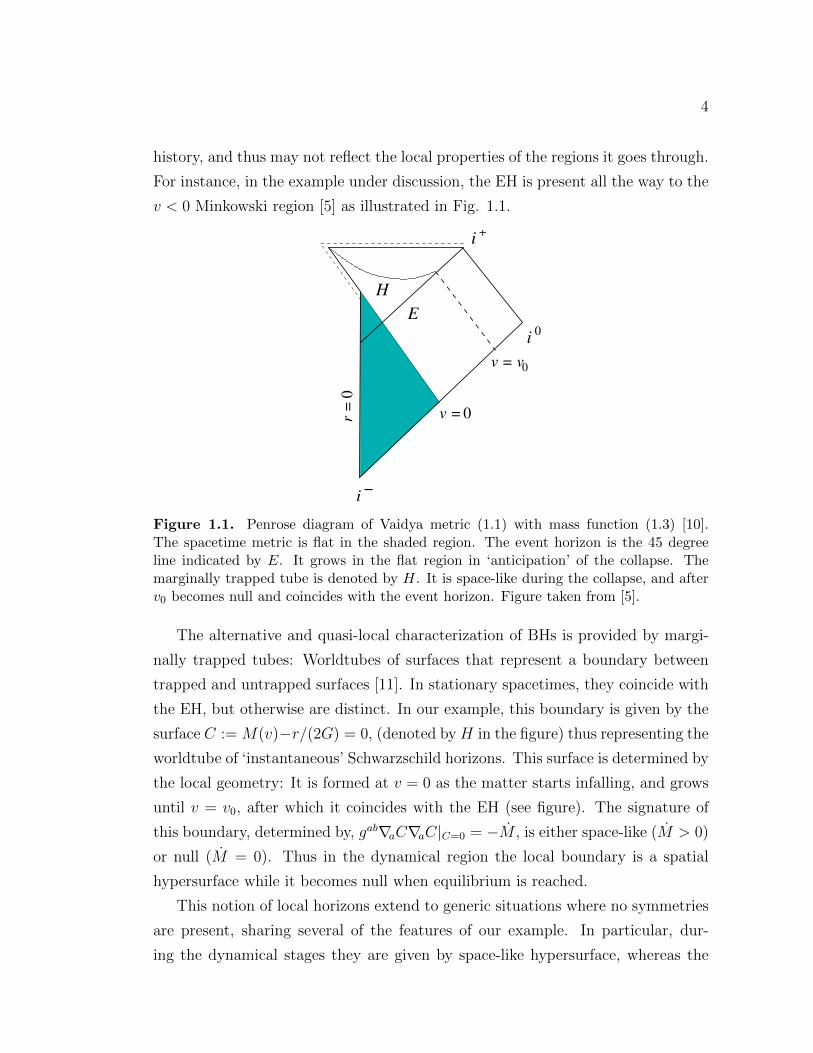
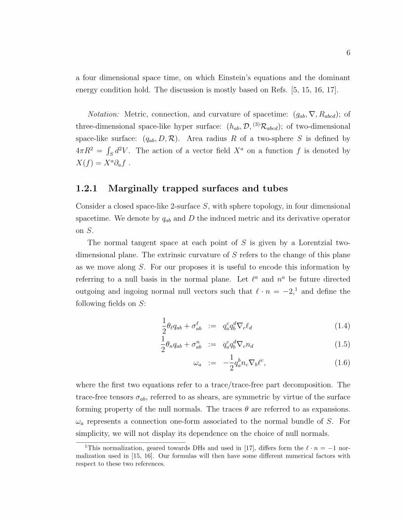
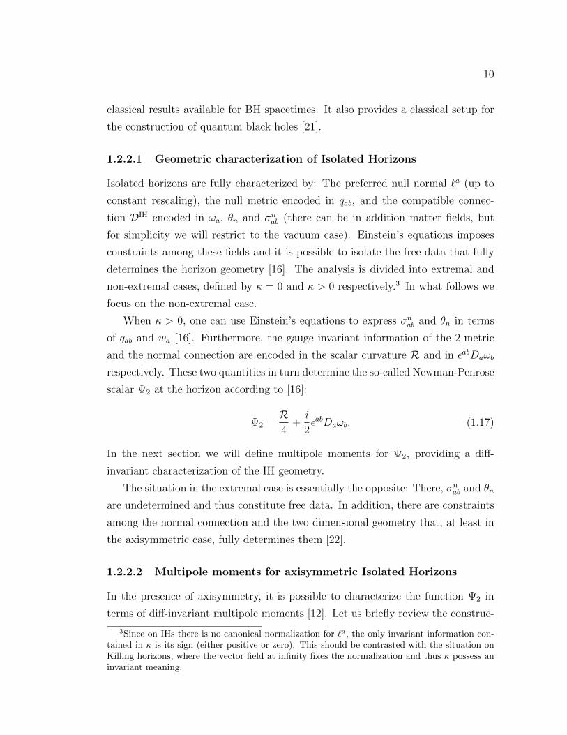
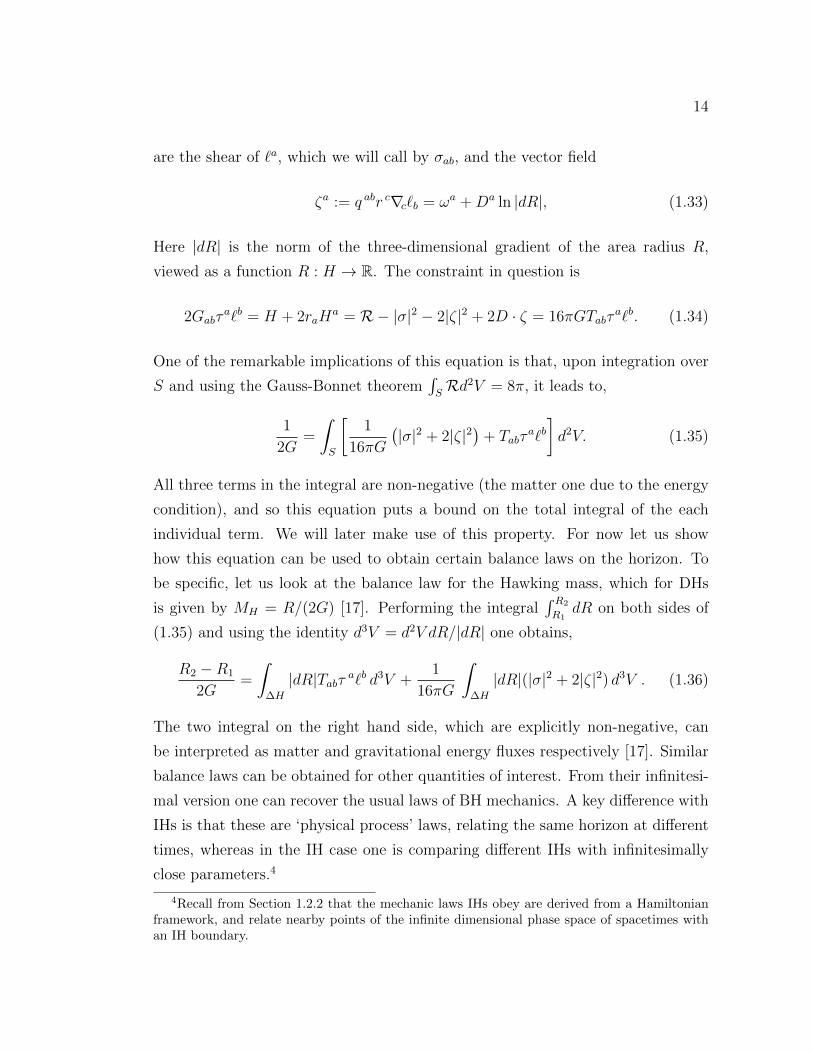
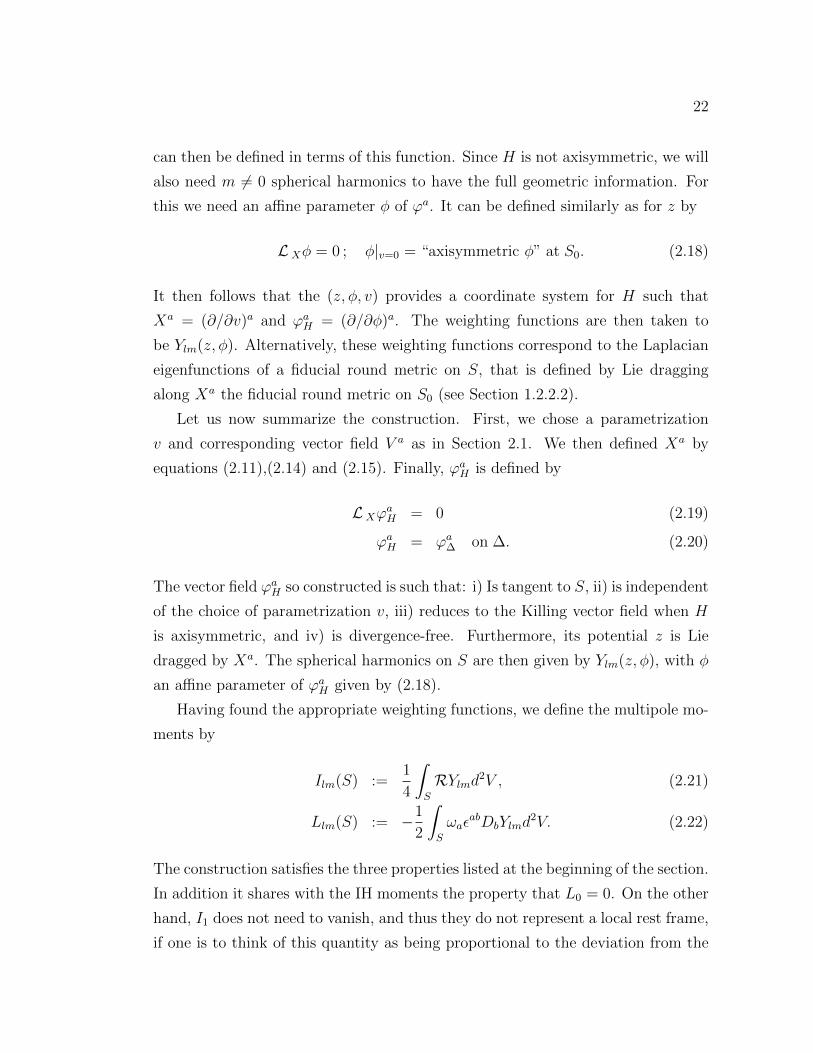
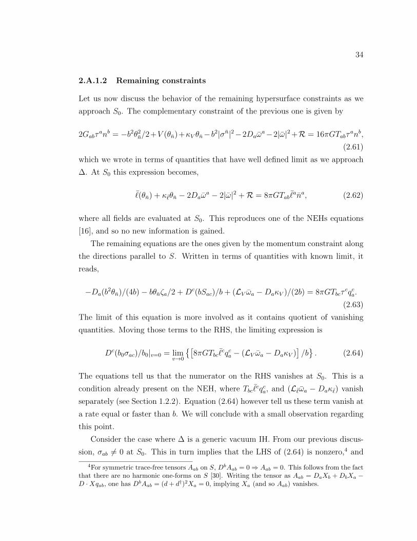
v < 0 Minkowski region [5] as illustrated in Fig. 1.1.

i+

i−

i0

v = v0

v = 0

E

r =

0

H

Figure 1.1. Penrose diagram of Vaidya metric (1.1) with mass function (1.3) [10].The spacetime metric is flat in the shaded region. The event horizon is the 45 degreeline indicated by E. It grows in the flat region in ‘anticipation’ of the collapse. Themarginally trapped tube is denoted by H. It is space-like during the collapse, and afterv0 becomes null and coincides with the event horizon. Figure taken from [5].

The alternative and quasi-local characterization of BHs is provided by margi-

nally trapped tubes: Worldtubes of surfaces that represent a boundary between

trapped and untrapped surfaces [11]. In stationary spacetimes, they coincide with

the EH, but otherwise are distinct. In our example, this boundary is given by the

surface C := M(v)−r/(2G) = 0, (denoted by H in the figure) thus representing the

worldtube of ‘instantaneous’ Schwarzschild horizons. This surface is determined by

the local geometry: It is formed at v = 0 as the matter starts infalling, and grows

until v = v0, after which it coincides with the EH (see figure). The signature of

this boundary, determined by, gab∇aC∇aC|C=0 = −M , is either space-like (M > 0)

or null (M = 0). Thus in the dynamical region the local boundary is a spatial

hypersurface while it becomes null when equilibrium is reached.

This notion of local horizons extend to generic situations where no symmetries

are present, sharing several of the features of our example. In particular, dur-

ing the dynamical stages they are given by space-like hypersurface, whereas the

5

equilibrium stage is described by a null hypersurface. These are respectively the

notions of dynamical and isolated horizons we will review in the next section.

Describing the local horizon beyond the spherically symmetric case is however

more involved, as one needs to take into account all possible distortions on the

MTSs, as well as its local rotation. Here is where the notion of multipole moments

comes into picture.

Multipole moments for local horizons were introduced in the isolated case in

[12]. They provide a diffeomorphism invariant characterization of the horizon

geometry. Furthermore they have a physical interpretation of mass and angular

momentum multipoles moments, in an analogy with charge and current multipole

moments of classical electrodynamics. In the electrodynamics case, a localized

charge and current distribution, can be characterized by its multipole moments.

These description in turn facilitates the reconstruction of the electromagnetic field

outside the source: The source multipole moments determine, via field equations,

the field multipole moments, which characterize the 1/r expansion of fields, where r

is the distance to the source. Although such straightforward picture is not available

in the non-linear regime of GR we are interested in, there exists numerical evidence

for correlations between the horizon dynamics and the radiation at infinity [13, 14].

One of the ingredients needed to further explore such correlations is the availability

of an unambiguous notion of multipole moments for dynamical horizons.

Our aim will be to extend the notion of multipole moments from isolated to

dynamical horizons. This will provide a framework to invariantly describe the

evolving geometry of dynamical horizons, and a tool for studying the physics of

numerically evolved BHs.

1.2 Isolated and Dynamical Horizons

Isolated and Dynamical Horizons have quite distinct geometrical descriptions, as

they involve null and space-like hypersurfaces respectively. A common feature how-

ever is that they are both foliated by marginally trapped surfaces. Since we will

be eventually interested in the issue of the transition from a dynamical to isolated

horizon, we will make use of a description in terms of these marginally trapped

surfaces. Throughout our presentation, we will be dealing with submanifolds of

6

a four dimensional space time, on which Einstein’s equations and the dominant

energy condition hold. The discussion is mostly based on Refs. [5, 15, 16, 17].

Notation: Metric, connection, and curvature of spacetime: (gab,∇, Rabcd); of

three-dimensional space-like hyper surface: (hab,D, (3)Rabcd); of two-dimensional

space-like surface: (qab, D,R). Area radius R of a two-sphere S is defined by

4πR2 =∫Sd2V . The action of a vector field Xa on a function f is denoted by

X(f) = Xa∂af .

1.2.1 Marginally trapped surfaces and tubes

Consider a closed space-like 2-surface S, with sphere topology, in four dimensional

spacetime. We denote by qab and D the induced metric and its derivative operator

on S.

The normal tangent space at each point of S is given by a Lorentzial two-

dimensional plane. The extrinsic curvature of S refers to the change of this plane

as we move along S. For our proposes it is useful to encode this information by

referring to a null basis in the normal plane. Let `a and na be future directed

outgoing and ingoing normal null vectors such that ` · n = −2,1 and define the

following fields on S:

1

2θ`qab + σ`ab := qcaq

db∇c`d (1.4)

1

2θnqab + σnab := qcaq

db∇cnd (1.5)

ωa := −1

2qbanc∇b`

c, (1.6)

where the first two equations refer to a trace/trace-free part decomposition. The

trace-free tensors σab, referred to as shears, are symmetric by virtue of the surface

forming property of the null normals. The traces θ are referred to as expansions.

ωa represents a connection one-form associated to the normal bundle of S. For

simplicity, we will not display its dependence on the choice of null normals.

1This normalization, geared towards DHs and used in [17], differs form the ` · n = −1 nor-malization used in [15, 16]. Our formulas will then have some different numerical factors withrespect to these two references.

7

Given a different set of future directed null normals `′a and n′a, they will always

be related to the first ones by a local boost:

`′a = f`a

n′a = f−1na,(1.7)

for some function f > 0. The expansions and shears relate to each other by the

same multiplicative functions, whereas the normal connection transforms as

ω′a = ωa +Da ln f. (1.8)

If we think of the surface S as an instantaneous shell of light, then na and `a

represent the direction of the light rays going inside and outside the surface. In

regions of low curvature, θn < 0 and θ` > 0, meaning the light shells are respectively

contracting and expanding, as one would normally envisage such situation. In

strong curvature regimes however, it is possible for both expansions to be negative.

Such is the situation inside BHs. The limit case when θn < 0 and θ` = 0 is referred

to as marginally trapped surface (MTS). The notions of BH boundary we will

introduce refer to world tubes of these MTSs.

Consider then a three dimensional hypersurface H, of topology S2 × R, such

that it is foliated by MTSs. Let V a be a vector tangent to H and orthogonal to

the foliation. We will be interested in ‘future oriented tubes’ [15], for which V a

can be written as

V a = `a −B na (1.9)

for some choice of null normals and some function B. Since θ` = 0 everywhere on

H, it follows that V (θ`) = 0 so that

`(θ`) = B n(θ`). (1.10)

Let us now extend `a off H by a null geodesic congruence. The Raychaudhuri

equation evaluated at a point in the MTS, where θ` = 0, becomes

`(θ`) = −|σ`|2 −Rab`a`b. (1.11)

8

Einstein’s equations and the weak energy condition imply that the RHS of (1.11)

is non-positive. Substituting the LHS by (1.10) we obtain the inequality

B n(θ`) ≤ 0. (1.12)

If the surfaces immediately inside S are trapped (this was the motivation for

considering MTSs), then n(θ`) < 0 which implies B ≥ 0. Since V · V = B we

learn that H can be either space-like (B > 0) or null (B = 0). These are in fact

the only two possibilities, as shown for instance in [15]. The first case corresponds

to a DH, whereas the second to a non-expanding horizon (NEH). Finally, since

θ(V ) = −Bθn ≥ 0 we conclude that the area of the cross sections increases for

DHs and remains constant for NEHs. In these considerations we have assumed the

weak energy condition. If the energy condition were violated, as can be the case

in the presence of quantum fields, the RHS of (1.11) could be positive leading to

a time-like tube with decreasing area. This is what happens in the process of BH

evaporation by Hawking radiation [18].

We will now discuss the null and space-like cases separately.

1.2.2 NEHs and IHs

The first thing to notice in the null case is that `(θ`) = 0, which by equation (1.11)

implies σ`ab = 0 and Rab`a`b = 0. The vanishing of the expansion and shear of `a

is equivalent to

L `qab = 0 (1.13)

and so the metric is ‘time independent’. Rab`a`b = 0 implies, by Einstein’s equa-

tions and the energy condition, that Tab`b =∝ `a. This means that the matter

energy flux associated to the vector field `a is parallel to the horizon and so there

is no energy flux going across the horizon.

From the fact that H is null, it follows that ` is geodesic [1],

`b∇b`a = κ``

a, (1.14)

where κ`, called surface gravity, plays the role of BH temperature in the thermo-

dynamical interpretation [19]. So far nothing ensures that κ` is a constant, and

9

so a general NEH will not represent a BH in equilibrium. Notice however that κ`

depends on the choice of null normal. Under the rescaling (1.7), it transforms as

κ`′ = fκ` + `(f). (1.15)

In particular one can chose the null normal so that κ` is constant [16]. Inciden-

tally,this implies that the normal connection is time-independent, as follows form

the following identity of NEHs [16],

L `ωa = Daκ`. (1.16)

The condition of κ` being constant does not however uniquely fix `a. In [16] it is

shown that, on generic NEH,2 the additional condition `(θn) = 0 uniquely fixes a

preferred null normal (up to constant rescalings). Thus, under generic conditions,

every NEH has a preferred null normal (up to a multiplicative constant) obeying

L `ωa = 0 and `(θn) = 0. Such a horizon will have a ‘time independent’ geometry

except possibly for the components of the extrinsic geometry encoded in σnab to

which no condition has yet been imposed. When σnab is ‘time-independent’ the

NEH is said to be an isolated horizon (IH). To summarize, an IH is a NEH with

a preferred null normal `a which Lie-drags all extrinsic curvature components

(1.5,1.6).

Note: We have presented the concepts of NEH and IH using the auxiliary

structure of a foliation, in order to ease the transition to the next section. The

actual definitions of NEH and IH do not however refer to any foliation but directly

deal with the geometry of the null hypersurface. There, the objects of relevance

are, besides the null normal `a, a degenerate metric of signature (0,+,+) and a

connection DIH compatible with the metric (which is induced on the IH by the

spacetime connection). The fields ωa, θn and σnab from our presentation encode

the information of the connection DIH, and the IH requirement translates into the

condition [L `,DIH] = 0.

Let us conclude by mentioning that IHs can be used as space-time boundaries

in a canonical description of general relativity. Among other things, the frame-

work allows for a derivation of the BH mechanics equations [20], extending the

2A generic NEH is one where the operator given in equation (2.57) is invertible, see [16].

10

classical results available for BH spacetimes. It also provides a classical setup for

the construction of quantum black holes [21].

1.2.2.1 Geometric characterization of Isolated Horizons

Isolated horizons are fully characterized by: The preferred null normal `a (up to

constant rescaling), the null metric encoded in qab, and the compatible connec-

tion DIH encoded in ωa, θn and σnab (there can be in addition matter fields, but

for simplicity we will restrict to the vacuum case). Einstein’s equations imposes

constraints among these fields and it is possible to isolate the free data that fully

determines the horizon geometry [16]. The analysis is divided into extremal and

non-extremal cases, defined by κ = 0 and κ > 0 respectively.3 In what follows we

focus on the non-extremal case.

When κ > 0, one can use Einstein’s equations to express σnab and θn in terms

of qab and wa [16]. Furthermore, the gauge invariant information of the 2-metric

and the normal connection are encoded in the scalar curvature R and in εabDaωb

respectively. These two quantities in turn determine the so-called Newman-Penrose

scalar Ψ2 at the horizon according to [16]:

Ψ2 =R4

+i

2εabDaωb. (1.17)

In the next section we will define multipole moments for Ψ2, providing a diff-

invariant characterization of the IH geometry.

The situation in the extremal case is essentially the opposite: There, σnab and θn

are undetermined and thus constitute free data. In addition, there are constraints

among the normal connection and the two dimensional geometry that, at least in

the axisymmetric case, fully determines them [22].

1.2.2.2 Multipole moments for axisymmetric Isolated Horizons

In the presence of axisymmetry, it is possible to characterize the function Ψ2 in

terms of diff-invariant multipole moments [12]. Let us briefly review the construc-

3Since on IHs there is no canonical normalization for `a, the only invariant information con-tained in κ is its sign (either positive or zero). This should be contrasted with the situation onKilling horizons, where the vector field at infinity fixes the normalization and thus κ possess aninvariant meaning.

11

tion.

Consider a cross section S of the IH. The axisymmetry of the IH implies the

two dimensional metric qab posses a Killing vector field ϕa. The vector field in

particular preserves the area two-form εab and so can be written as

ϕa = R2εabDbz (1.18)

for some function z : S → R. Equation (1.18) determines z up to an additive

constant, which is fixed by requiring∫Szd2V = 0. One can further show that z

is monotonically increasing from one pole to the other, and its range is [−1, 1].

Together with an affine parameter φ of ϕa, one obtains a canonical (up to a global

rotation) coordinate system (z, φ) on S, in terms of which the metric takes the

form

qabdxadxb = R2(f−1dz2 + fdφ2), (1.19)

with f = f(z) such that f(±1) = 0 and f ′(±1) = ∓2. The scalar curvature is

then given by

R(z, φ) = −f′′(z)

R2. (1.20)

As an example and for later reference, for the Kerr horizon of parameters a and

r (where the angular momentum is proportional to a ∈ [0, r], and R2 = r2 + a2),

the metric qab is given by the function

fa(z) :=(r2 + a2)

r2 + a2z2(1− z2). (1.21)

In particular fa=0(z) = (1 − z2) represents the round sphere metric, where usual

spherical coordinates are recovered by setting z = cos θ.

Given the axisymmetric metric qab on S, using z and φ one can construct a

canonical fiducial round metric by

qabdxadxb := R2(f−1

0 dz2 + f0dφ2). (1.22)

Its corresponding spherical harmonics Ylm are the ones used as weighting func-

tions to define the multipole moments. Because of axisymmetry, only the m = 0

12

moments are non-zero. They are defined as

Il := 14

∫SRYl0d2V =

∫S

ReΨ2Yl0d2V,

Ll := −12

∫Sωaε

abDbYl0d2V = −

∫S

ImΨ2Yl0d2V,

(1.23)

corresponding to the decomposition

Ψ2 =1

R2

∞∑l=0

(Il − iLl)Yl0. (1.24)

Summarizing, the geometric multipole moments (1.23) are constructed using the

structure available from the axisymmetry, providing a set of diff-invariant quanti-

ties that fully characterize horizon geometry (see [12] for the explicit reconstruction

of the IH geometry from a given set of multipole moments).

The geometric moments (1.23) can also be used to define ‘mass’ and ‘angular

momentum’ multipoles in an an analogy with charge and current multipoles of

electromagnetism [12]:

Jl =√

4π2l+1

Rl+1

4πGLl,

Ml =√

4π2l+1

MRl

2πIl.

(1.25)

The normalizations are such that J1 agrees with the angular momentum as defined

by either the Komar integral or the Hamiltonian framework, and

M0 = M :=1

2GR

√R4 + 4G2J1 (1.26)

reproduces the mass of a Kerr black hole of radius R and angular momentum J1.

From their definitions it follows that the angular momentum monopole J0, as

well as the mass dipole M1 vanish. The first property implies that the IH does not

have NUT charge, while in a Newtonian interpretation, the second implies one is

working in the center of mass frame.

1.2.3 Dynamical Horizons

The case when the worldtube H of MTSs is space-like is known as a dynamical

horizon [17]. Since H is space-like, it has a unit time-like normal τa and its

geometry is encoded in the metric hab = gab + τaτb, of signature (+,+,+), and

13

extrinsic curvature Kab := hachb

d∇cτd. Einstein equations impose the hypersurface

constraints:

H := 2Gabτaτ b = (3)R+K2 −KabKab = 16πGTab τ

aτ b (1.27)

Ha := Gbcτbhab = Db

(Kab −Khab

)= 8πGT bc τ ch

ab , (1.28)

where Gab = Rab − 1/2Rgab, D is the connection of hab,(3)R its scalar curvature

and Tab the stress-energy tensor.

The foliation by MTSs induces a ‘2+1’ splitting of H. Let ra be the unit vector

tangent to H and orthogonal to the foliation. The two dimensional metric qab on

S is then related to the three-metric by

hab = qab + rarb. (1.29)

We will denote by Kab := qacqb

dDcrd the extrinsic curvature of S within H. Finally,

we decompose the extrinsic curvature of H as

Kab = Aqab + Sab + 2ω(arb) +Brarb , (1.30)

where Sab is parallel to S and trace-free, and ωa is parallel to S. In the language of

Section 1.2.1, the vector ωa corresponds to the connection one-form (1.6) associated

to the null normals`a := τa + ra ,

na := τa − ra.(1.31)

The expansion of ` is given by θ` = 2A+K where K = qabKab and so the marginally

trapped condition translates into

A = −K/2. (1.32)

As shown in [17], condition (1.32) has the surprising consequence that one of

the hypersurface constraints involves only derivatives along S, and thus provides

an ‘instantaneous’ constraint for each leaf S. The fields featuring this constraint

14

are the shear of `a, which we will call by σab, and the vector field

ζa := q abr c∇c`b = ωa +Da ln |dR|, (1.33)

Here |dR| is the norm of the three-dimensional gradient of the area radius R,

viewed as a function R : H → R. The constraint in question is

2Gabτa`b = H + 2raH

a = R− |σ|2 − 2|ζ|2 + 2D · ζ = 16πGTabτa`b. (1.34)

One of the remarkable implications of this equation is that, upon integration over

S and using the Gauss-Bonnet theorem∫SRd2V = 8π, it leads to,

1

2G=

∫S

[1

16πG

(|σ|2 + 2|ζ|2

)+ Tabτ

a`b]d2V. (1.35)

All three terms in the integral are non-negative (the matter one due to the energy

condition), and so this equation puts a bound on the total integral of the each

individual term. We will later make use of this property. For now let us show

how this equation can be used to obtain certain balance laws on the horizon. To

be specific, let us look at the balance law for the Hawking mass, which for DHs

is given by MH = R/(2G) [17]. Performing the integral∫ R2

R1dR on both sides of

(1.35) and using the identity d3V = d2V dR/|dR| one obtains,

R2 −R1

2G=

∫∆H

|dR|Tabτ a`b d3V +1

16πG

∫∆H

|dR|(|σ|2 + 2|ζ|2) d3V . (1.36)

The two integral on the right hand side, which are explicitly non-negative, can

be interpreted as matter and gravitational energy fluxes respectively [17]. Similar

balance laws can be obtained for other quantities of interest. From their infinitesi-

mal version one can recover the usual laws of BH mechanics. A key difference with

IHs is that these are ‘physical process’ laws, relating the same horizon at different

times, whereas in the IH case one is comparing different IHs with infinitesimally

close parameters.4

4Recall from Section 1.2.2 that the mechanic laws IHs obey are derived from a Hamiltonianframework, and relate nearby points of the infinite dimensional phase space of spacetimes withan IH boundary.

15

We conclude the section by recalling the balance law for angular momentum. In

general, the notion of angular momentum is associated to the presence of axisym-

metry. One can however have a generalized notion of angular momentum associ-

ated to any vector field ϕa that is tangent to the cross sections S and divergence-

free thereon. It is defined by the same expression one would get in the presence of

axisymmetry:

JϕS := − 1

8πG

∫S

Kabϕarb d2V (1.37)

= − 1

8πG

∫S

ωaϕa d2V, (1.38)

where the second equality follows from the decomposition of the extrinsic curvature

(1.30). The balance law for ∆Jϕ is obtained by using i) Stokes theorem to express

the difference as an integral over the bounded volume ∆H, and ii) the momentum

constraint (1.28). The result is

∆Jϕ = −∫

∆H

Tabτaϕb d3V − 1

16πG

∫∆H

P abL ϕhab d3V (1.39)

where Pab = Kab −Khab. The two integrals are respectively interpreted as matter

and gravitational angular momentum fluxes. In particular the gravitational angu-

lar momentum flux vanishes when ϕa is Killing vector field of the intrinsic metric

hab on H.

Chapter 2Multipole moments of DHs and

Approach to equilibrium

Having introduce both isolated and dynamical horizons, we now focus on the in-

terface between the two concepts. Specifically, we will explore the passage from

dynamical to isolated horizon, and use the final equilibrium state as a ‘reference

frame’ with respect to which the evolving geometry of the DH can be described.

As discussed in the first chapter, the final equilibrium of dynamical black holes

is given by a Kerr BH. In the context of IHs however, the Kerr family is one in

many possible horizons. Its special status only comes when one considers the whole

spacetime, or at least some region enclosing the horizon.

Our strategy will be to include this additional information and thus focus on

DHs that settle to a final Kerr horizon.

We will first discuss the general issue of passage from dynamical to isolated

horizon and then present the construction of multipole moments, which provide

an invariant characterization of the settling process.

2.1 Dynamical to Isolated transition

As mentioned at the end of Section 1.2.1, one of the properties of marginally

trapped tubes is that they have definite signature along each cross section [15].

This implies the transition from dynamical to isolated horizon occurs at an ‘instant’

surface S0. This transition can either happen at finite time or be asymptotic.

17

Most of what follows applies to both cases, but for concreteness we will center the

discussion in the case where the transition happens at ‘finite time’. Consider then

a worldtube of MTSs M := H ∪∆ consisting of the union of a dynamical horizon

H and a non-expanding horizon ∆. We will eventually be interested in the case

where ∆ is a Kerr horizon, but the following discussion applies to general NEHs.1

We will assume M and the spacetime metric to be smooth.

We fix once and for all a null normal ¯a of the NEH ∆ (in the IH case we may

chose it to belong to the preferred class, but otherwise we leave it general). NEHs

do not have an a priori foliation. In the present setting however, the initial surface

S0 induces a foliation given by v : ∆ → [0,∞) such that ¯(v) = 1 and v = 0 on

S0. We will denote by na the ingoing null normal orthogonal to the foliation such

that ¯· n = −2.

To study the transition H → ∆, we introduce a smooth foliation function

v : M → R on the total horizon M such that it agrees with v for v > 0. Thus,

v =constant< 0 gives the leaves of the DH, v =constant> 0 gives the leaves of the

NEH, and v = 0 represents the transition surface S0. The freedom in the choice of

such foliation function is given by ‘time reparametrizations’: Given another choice

w, there exists a smooth function f such that w = f(v), with f(v) = v for v ≥ 0.

Our construction of multipole moments of Section 2.2 will be independent of this

reparametrization freedom.

A foliation v uniquely determines a vector field V a satisfying: i) V a is tangent

to M and orthogonal to the cross sections, ii) V (v) = 1. These conditions imply

that V a coincides with ¯a on ∆, and so it represents a smooth extension of this

vector field to H. On H, V a is proportional to ra:

V a = |dv|−1ra =: 2b ra, (2.1)

where for later convenience b is defined by

2b = |dv|−1 = R|dR|−1; R ≡ dR

dv, (2.2)

1There could in principle be a situation where the equilibrium is reached in stages: first DHto NEH and then NEH to IH.

18

or equivalently

V · V = 4 b2. (2.3)

This last equation tell us that b smoothly vanishes at S0. If b is used to rescale the

null normals (1.31) according to

¯aH := b `a (2.4)

naH := b−1na, (2.5)

one obtains smooth extensions of the NEH null normals. This is seen by writing

b `a = V a + b na in (2.4), which becomes ¯a at S0. The ingoing null normal is then

uniquely determined by the normalization condition ¯H · nH = −2. From now on

we drop the subscript H and denote by ¯a and na the total vector fields on M .

The condition that at S0 we have a given NEH determines the limiting value

of the shears, expansions and normal connection (1.4,1.4,1.6) of the null normals

(2.4), (2.5).

Some of the conclusions that can be obtained about the transition are:

• |σ|2 and Tabτa`b, featuring in the energy flux formula (1.36), have finite limits

at S0. Furthermore, for generic ∆, |σ|2 and Tabτa`b cannot simultaneously

vanish at S0. The energy flux in (1.36) still vanishes at S0 due to the |dR|factor.

• b2 vanishes as R. That is,

b0 :=b√R

(2.6)

is a well defined function on H admitting a regular non-vanishing limit to

S0. Furthermore, the limiting value b0|v=0 is related to the limiting value of

the divergence of ζa.

• The trace of the extrinsic curvature diverges at S0. In particular, the ‘con-

stant mean curvature’ strategy for solving the constraint equations [23] can-

not be applied to DHs approaching equilibrium.

We leave the proof of these properties to the appendix. As an example for the

first two points, in the Vaidya collapse one has b0 = 1/√

2 (with respect to the

coordinate v of (1.1)) and 8πGTab`aτ b = 1/R2 [17].

19

2.2 Multipole moments for Dynamical Horizons

We saw in Section 1.2.2.2 how multipole moments of IHs provide a diff-invariant

characterization of the horizon geometry. We would like to extend this notion to

DHs, in order to have a framework to describe the approach to equilibrium in an

invariant manner.

Here is where we want to use the additional information that the final equilib-

rium is given by a Kerr horizon. The only property of the Kerr horizon we will

actually need however is its axisymmetry. Thus our setup will be as in the previous

section, with a total horizon of the form M = H ∪∆, with ∆ an axisymmetric IH.

Let us first consider the situation where H is also axisymmetric (and hence the

total horizon M is axisymmetric). In this case it is straightforward to extend the

definition of IH multipole moments to DHs [7]: On each DH cross section S, the

multipole moments are simply defined to be

Il(S) := 14

∫SRYl0d2V

Ll(S) := −12

∫Sωaε

abDbYl0d2V,

(2.7)

where the spherical harmonics are defined by reproducing the construction of sec-

tion 1.2.2.2 on each cross section S. These functions will be generically ‘time de-

pendent’ in the sense that they will depend on the cross section, and will smoothly

match with the multipole moments of the IH ∆ at S0.

Let us now go to the general case where H is not necessarily axisymmetric, but

still with final axisymmetric ∆. Since now there is no intrinsic structure on S that

can be used to define the spherical harmonics, the strategy will be to bring down

to S the spherical harmonics available at ∆. A satisfactory construction should be

such that:

1. It is diff-invariant: It does not depend on choices of auxiliary structures

2. It should reduce to (2.7), when H is axisymmetric

3. The DH multipole moments should smoothly match the IH ones at S0

How can this be achieved? In the axisymmetric case, the weighting functions

Y (z)l0 are defined in terms of the ‘potential’ z of the Killing vector field ϕa, Eq.

20

(1.18). The idea is to repeat this construction with respect to a vector field ϕaH on

H which may not be Killing, but still of the form

R2εabDbz = ϕaH , (2.8)

for some function z. This vector field should be uniquely determined by the avail-

able structure (a DH H ending in an axisymmetric IH ∆) and should reproduce

the Killing vector field whenever H is axisymmetric.

We will seek such ϕaH by transporting the axisymmetric vector field ϕa∆ on ∆

to H. A first guess is to define it by the following conditions:

L V ϕaH = 0 (tentative) (2.9)

ϕaH = ϕa∆ on ∆ , (2.10)

with V a given by (2.1). This definition has the following desirables properties:

i) ϕaH is tangent to H since (2.9) implies ϕH(v) is constant, and by (2.10) this

constant is zero.

ii) ϕaH is independent of the chosen parametrization: Given a different parame-

trization w = f(v), the corresponding vector field is given by W a = f−1V a, which

in turn implies L V ϕaH = 0 ⇐⇒ LWϕ

aH = 0.

iii) If H is axisymmetric, ϕaH coincides with the Killing vector field ϕa: Ax-

isymmetry implies L ϕV = 0, and so ϕa obeys (2.9). Since it also obeys (2.10), it

follows that ϕaH = ϕa.

This construction however is not satisfactory as it fails in a fourth fundamental

requirement: It does not guarantee that D · ϕH = 0, the condition needed to have

a ‘potential’ z (1.18). This can be fixed by adding an appropriately ‘shift’ to the

vector field V a used to transport ϕaH from ∆ to H. Thus consider a vector field of

the form

Xa = V a +Na, (2.11)

with Na tangent to S, and consider now ϕaH defined as before but with Xa in place

of V a. Clearly property i) above still holds. We then need to find Na such that

properties ii), iii) and the additional condition iv) D · ϕH = 0, are satisfied.

21

Let us focus on the fourth property. Recall the notion of divergence does not

require knowledge of the total metric but only of the area element: L ϕH εab =

(D ·ϕH)εab. Furthermore, the notion of vanishing divergence makes use of the area

element up to global rescalings. Thus, if the change of εab along Xa is of the form

LXεab = a(v)εab for some function a(v), the divergence of ϕaH will remain constant

and thus will be zero since it vanishes on ∆. The condition that the total integral

of εab/R2 is constant determines a = 2R/R. The required vector field Xa should

then satisfy:

LXεab = 2R/Rεab , or, LX(εab/R2) = 0. (2.12)

The change in the area element along a vector field of the form (2.11) is given by

LXεab = (2bK +D ·N)εab, (2.13)

where we used (2.1) and L rεab = Kεab, with K the trace of the extrinsic curvature

of S ⊂ H (see Section 1.2.3). Thus, by taking

Na = Dag, (2.14)

with g satisfying

−∆g = 2R/R− 2 b K, (2.15)

one obtains a vector field obeying (2.12). Note that, given v, this Na is unique

and its construction is diffeomorphism invariant.

This prescription satisfies ii), since under reparametrization, Na transforms as

V a:

v → f(v) ⇒ Na → f−1Na. (2.16)

Finally, if H is axisymmetric, then we are guaranteed to have L ϕNa = 0, whence

property iii) will be satisfied. We thus have a successful candidate for ϕaH . Let us

now explore further consequences. First, one can verify that the function z defined

by

LXz = 0 ; z|v=0 = “axisymmetric z” at S0 (2.17)

is a potential for ϕaH in the sense of Eq. (2.8), and so has the same properties as in

∆: Integrates to zero on S and its range is [−1, 1]. The m = 0 spherical harmonics

22

can then be defined in terms of this function. Since H is not axisymmetric, we will

also need m 6= 0 spherical harmonics to have the full geometric information. For

this we need an affine parameter φ of ϕa. It can be defined similarly as for z by

LXφ = 0 ; φ|v=0 = “axisymmetric φ” at S0. (2.18)

It then follows that the (z, φ, v) provides a coordinate system for H such that

Xa = (∂/∂v)a and ϕaH = (∂/∂φ)a. The weighting functions are then taken to

be Ylm(z, φ). Alternatively, these weighting functions correspond to the Laplacian

eigenfunctions of a fiducial round metric on S, that is defined by Lie dragging

along Xa the fiducial round metric on S0 (see Section 1.2.2.2).

Let us now summarize the construction. First, we chose a parametrization

v and corresponding vector field V a as in Section 2.1. We then defined Xa by

equations (2.11),(2.14) and (2.15). Finally, ϕaH is defined by

LXϕaH = 0 (2.19)

ϕaH = ϕa∆ on ∆. (2.20)

The vector field ϕaH so constructed is such that: i) Is tangent to S, ii) is independent

of the choice of parametrization v, iii) reduces to the Killing vector field when H

is axisymmetric, and iv) is divergence-free. Furthermore, its potential z is Lie

dragged by Xa. The spherical harmonics on S are then given by Ylm(z, φ), with φ

an affine parameter of ϕaH given by (2.18).

Having found the appropriate weighting functions, we define the multipole mo-

ments by

Ilm(S) :=1

4

∫S

RYlmd2V , (2.21)

Llm(S) := −1

2

∫S

ωaεabDbYlmd

2V. (2.22)

The construction satisfies the three properties listed at the beginning of the section.

In addition it shares with the IH moments the property that L0 = 0. On the other

hand, I1 does not need to vanish, and thus they do not represent a local rest frame,

if one is to think of this quantity as being proportional to the deviation from the

23

center of mass (see Section 1.2.2.2). This is compatible with the the interpretation

that these are the multipoles from the perspective of the final equilibrium state,

whose center of mass may have shifted.

Note that the above represent the analogues of the isolated horizon geometric

moments (1.23). The so-called physical moments can be obtained by appropriate

constant rescaling as in (1.25).

We now discuss possible balance laws for these multipole moments, and com-

pare our construction with others available in the literature.

2.2.1 Balance laws for Multipole moments

In Section 1.2.3, we mentioned certain balance laws that hold on DHs. In particular

we looked at a ‘mass’ (1.36) and angular momentum (1.39) balance laws expressing

the change of these quantities in terms of fluxes across the horizon. We now seek

for similar balance laws for the multipole moments introduced before.

We will for simplicity focus on the geometric moments (2.21), (2.22), but similar

balance laws can be obtained for the physical moments by including the appropriate

factors.

Let us start with the angular moments. We observe that expression (2.22) has

the same form as the generalized angular momentum (1.38), with respect to the

vector field

ϕalm := εabDbYlm, (2.23)

namely

Llm(S) = 4πGJϕlmS , (2.24)

with JS as defined in (1.38). Thus, up to a proportionality factor, the multipole

moments (2.22) can be thought of as giving the generalized angular momenta

corresponding to the divergence-free (in S) vector fields (2.23). In particular, we

can repeat the analysis leading to angular momentum balance law (1.39). Using

(2.24) and (1.39), we obtain

LS2lm − L

S1lm = −

∫∆H

(4πGTabτ

aϕblm +1

4P abL ϕlmhab

)d3V, (2.25)

where ∆H is the portion of H bounded by the two surfaces. The interpretation of

24

this equation is as before: The angular moments change in response of matter and

geometric fluxes across the horizon, given by the first and second terms in (2.25)

respectively. The fluxes depend on the order of the moment, and in particular they

vanish for l = 0, which is consistent with the fact that L0 = 0.

We now turn to the Ilm moments. Here we would like to proceed in a similar

spirit as for the DH ‘mass’ balance law (1.36). In particular, we will seek to

express the change in moments in terms of the energy fluxes featuring (1.36).

Notice however that we are dealing with the geometric (rather than ‘physical’)

moments. In particular I0 =√π =constant. We start by writing the difference as

IS2lm − I

S1lm =

∫dR

dIlmdR

. (2.26)

Now, let (∂/∂R)a = R−1Xa be the vector field associated to the coordinate system

(R, z, φ). We then have

dIlmdR

=1

4

∫S

L ∂/∂R(RYlmεab) (2.27)

=1

4

∫S

(2

RR+ ∂RR)Ylmd

2V , (2.28)

where we used L ∂/∂Rεab = 2Rεab and ∂Ylm/∂R = 0. In order to bring in the flux

terms, we use Eq. (1.34), to express R in terms of the radiative quantities. Doing

so for the first term in (2.28) we obtain,

dIlmdR

=1

2R

∫S

Ylm(|σ|2 + 2|ζ|2 + 16πGTabτa`b − 2D · ζ)d2V +

1

4

∫S

Ylm∂RRd2V.

(2.29)

We finally integrate over R and rearrange terms to obtain:

IS2lm − I

S1lm =

∫∆H

|dR|2R

(|σ|2 + 2|ζ|2 + 16πGTabτ

a`b)Ylmd

3V (2.30)

+∫

∆H|dR|

(1

4Ylm ∂RR+

1

Rζ(Ylm)

)d3V, (2.31)

where we collected in the first integral the contribution from the gravitational and

matter flux-like terms, weighted by the Ylm factors. The remaining terms, collected

in the second integral, have a less immediate interpretation. Their presence is

25

however necessary, as can bee seen by looking at the l = 0 case, where they must

cancel the positive contribution of the flux integral (recall I0 = constant).

We conclude by exploring an alternative expression for the change of the mul-

tipole moments which exhibits certain symmetry between both sets of moments.

We begin with the angular moments. Recall from the earlier discussion that

they can thought of as generalized angular momentum with respect to the vector

field (2.23):

Llm = −1

2

∫S

ωaϕalmd

2V. (2.32)

The vector fields ϕalm form a basis in the space of divergence-free vector fields of

S, and thus from (2.32) one can reconstruct the generalized angular momentum

with respect to any divergence-free vector field.

We now focus on the rate of change of Llm with respect to the parameter v of

the previous section and write

dLlmdv

= −1

2

∫S

LX(ωcϕclmεab), (2.33)

= −1

2

∫S

LX(ωc)ϕclmεab −

1

2

∫S

ωcLX(ϕclmεab). (2.34)

The second term is vanishing, since

ϕclmεab = εcdDdYlmεab = (R2εcd)(DdYlm)(R−2εab), (2.35)

and each term in parenthesis is Lie dragged by Xa. We thus conclude that

dLlmdv

= −1

2

∫S

ϕalmLXωa d2V. (2.36)

Remarkably, a similar expression holds for the mass moments. This comes from

the fact that one can locally write the scalar curvature as R = 2εabDaΓb, where

Γa is the so(2) connection associated to an orthonormal dyad. In order to deal

with the fact that Γa is not globally defined, consider the fiducial round round

metric qab on S (defined by Lie dragging along Xa the fiducial round metric at S0,

see Section 2.2). The multipole moments associated to the round metric are all

26

vanishing for l > 0 [12]. We can thus write

Ilm(S) =1

4

∫S

(R− R)Ylmd2V, l > 0. (2.37)

The advantage of this rewriting is that now there exist a globally defined one-form

Ca, such that (R−R) = 2εabDaCb (roughly speaking, Ca is given by the difference

between Γa and Γa). The ‘mass’ moments then take the same form as the angular

moments (2.32):

Ilm =1

2

∫S

Caϕalmd

2V, l > 0. (2.38)

In particular, the moments do not depend on any gradient ambiguity in Ca. Pro-

ceeding as with the angular moments, we conclude that

dIlmdv

=1

2

∫S

ϕalmLXCa d2V, (2.39)

where the equation is now valid for l ≥ 0, for it gives the correct vanishing result

for l = 0.

2.2.2 Relation with other approaches

Robert Owen [8] has defined multipole moments by expanding R and εabDaωb with

respect to a different set of basis functions. These are defined as eigenfunctions of

a generalized Laplacian, with the property that, in the presence of axisymmetry,

one recovers the potential z of the Killing field (1.18). In the axisymmetric case,

the zeroth and first angular moments coincides with the ones defined here, but for

higher multipoles, the moments will be related to ours by some time-dependent

linear transformation.

The advantage of Owen’s approach is that moments are defined locally, and

so there is no need to refer to the final equilibrium state. On the other hand the

basis functions he uses are themselves time dependent. This makes it somewhat

difficult to attribute direct physical meaning to the difference between moments

evaluated at different times. This is to be contrasted to our approach where the ba-

sis functions are time-independent and refer to the final equilibrium state, making

it clearer for the comparison of moments at different times.

27

Let us now bring to attention a subtle point we did not touch upon. The

multipole moments for IHs are usually stated in terms of the real and imaginary

parts of Ψ2. For DHs however, these quantities are not simply given by R and

εabDaωb , but rather one has (vacuum case):

ReΨ2 =1

4

(R+ qabqcdσ`acσ

nbd

)(2.40)

ImΨ2 =1

4

(2 εabDaωb − εabqcdσ`acσnbd

). (2.41)

When the DH becomes null, the shear terms vanish and one recovers the relation

(1.17). But on the dynamical side, which quantity shall one use to define multipole

moments? The choice we made puts emphasis on the geometry of the horizon

itself, rather than in the Newman-Penrose components of the spacetime curvature.

However, there is also the approach based on the use of ‘tendexes and vortexes

lines’ to visualize spacetime curvature [24, 25]. There, curvature is represented

through the integral lines of the eigendirections of the electric and magnetic Weyl

curvature tensors,

Eab = Cacbdτcτ d, (2.42)

Bab = ?Cacbdτcτ d =

1

2ε pqac Cpqbdτ

cτ d, (2.43)

in a given 3+1 foliation of spacetime (Cabcd is the Weyl tensor and τa refer to the

unit time-like normal to the foliation hypersurfaces Σ). In the presence of a BH,

these lines cross the MTS. At this surface, the normal components of the electric

and magnetic tensors act as sources for these lines, providing a qualitative picture

for the interaction of the BH with gravitational radiation [24]. These normal

components are nothing but the real and imaginary part of Ψ2,

Ψ2 =1

2(Eabr

arb + iBabrarb) , (2.44)

where ra denotes the space-like unit normal of the MTS in Σ. Note however that

this Ψ2 refers to the choice of foliation Σ which is quite arbitrary in dynamical

situations. Therefore, beyond the Kerr solution on which much of the intuition is

based in this approach, the invariant significance of the approach to equilibrium

28

via dynamics of tendexes and vortexes remains illusive.

2.3 Discussion

There is both theoretical and numerical evidence that the final equilibrium state

of dynamical BHs is given by the Kerr solution. This result cannot be derived

purely within the framework of local horizons, since the Kerr horizon is just a two-

parameter family in an infinite-dimensional space of possible IHs. However, as we

have shown, if this information is fed into the local description, one can obtain a

very detailed, diffeomorphism invariant description of the approach to equilibrium,

which has remained poorly understood thus far.

The Kerr horizon is well understood from the perspective of isolated horizons:

It posses an intrinsic characterization [26], and can be represented in terms of

specific multipole moments [12]. As a BH is formed by a gravitational collapse

or a merger of two BHs, the question then is: How is the final equilibrium state

reached?

To address this issue we constructed an analytical framework to extract the

strong field physics of the approach to equilibrium. We presented a way to in-

variantly describe the DH evolving geometry by extending the notion of multipole

moments of IHs to DHs. The constraint equations then imply certain balance laws

these moments obey. In the process, we also analyzed the conceptually subtle tran-

sition from the space-like dynamical horizon to the null isolated horizon, finding

the asymptotic behavior of fields as the transition surface is approached. In par-

ticular, our dynamical horizon multipole moments were shown to tend to those of

the isolated horizon, i.e., the Kerr horizon multipoles in situations of astrophysical

interest.

There are several phenomena associated to BHs that have been discovered

through numerical relativity. These include, the critical behavior in gravitational

collapse [27], and the occurrence of so-called kicks in the collision of BHs [28]. Our

framework provides the tools to formulate new questions in numerical relativity:

How do the multipole moments settle to the final Kerr value as a function of the

horizon radius? Are there universal features in such process? The number of

numerical simulations of BH merges is growing very rapidly and our framework

29

can be readily used to extract the coordinate independent physical information

from the last stages of these numerical evolutions. It is possible an interplay

between our analytical methods and numerics will shed new light on how diverse

dynamical horizon geometries finally settle down to the same geometry, given by

the Kerr isolated horizon. Finally, the balance law identities provide non-trivial

checks for the numerical simulations.

Our results also open new avenues for further theoretical investigations. We

conclude with two examples.

Part of the motivation in studying dynamical BHs is given by the prospects

of measuring their emitted gravitational waves. However, the relation between

DHs and gravitational waves is more subtle than one’s initial picture. For, DHs

lie inside the EH and thus cannot be the source of the gravitational radiation at

infinity. Nevertheless there do exist correlations between the evolution of the DH

and the gravitational radiation at infinity. In particular, a research program aimed

at understanding and exploiting these correlations is currently being pursued by

Jaramillo et.al. [14]. Our framework provides a more compete conceptual arena

for such analyses. Among other things, our results are likely to reduce the gauge

ambiguities that are present in this and related investigations.

Finally, in Section 1.2.2.1 we discussed the free data of IHs, and later show how

the multipole moments encode such information. The analogue of this problem

for DH remains open:2 Find a set of freely specifiable data which, through the

DH equations, allow one to reconstruct the full horizon geometry. The multipole

moments of DHs could offer a new perspective to this problem.

2.A Appendix: Limiting behavior at S0

In this appendix, we show the properties enunciated in Section 2.1 and discuss the

limit to S0 of the constraint equations.

Equation (1.35), tell us that |σ|2, |ζ|2 and Tabτa`b (which is positive due to

the energy condition) remain bounded as we approach S0, and so we conclude

that σab, ζa and Tabτa`b have well defined limits at S0. While analyzing the con-

straint at S0 we will see that for generic NEHs these two quantities cannot vanish

2Except in the special case of spherically symmetric DHs [29].

30

simultaneously.

To show the relation between b and R, we start by expressing the rate of change

in the area A ≡ dA/dv as

A =

∫Sv

LV (εab) . (2.45)

Writing the RHS integrand as LV εab = − b2θnεab, and expressing A in terms of R,

equation (2.45) takes the form 8πRR = −∫Svb2θnd

2V , from which we obtain,

limv→0

∫Sv

b2

Rθnd

2V = −8πR0, (2.46)

with R0 is the areal radius of S0. Since the integrand in (2.46) is strictly negative

and θn → θ(0)n has a well defined limit, it follows that

b0 =b√R

(2.47)

is a well defined function on H admitting a regular non vanishing limit to S0. We

thus conclude that b2 vanishes at the same rate as R does:

b2 ∼ R b20, for v → 0. (2.48)

To show the relation of the limiting values of b0 and ζa, we decompose the

vector into its curl/divergence free components:

ζa = −Da(lnu) + sa, (2.49)

where u > 0 is unique up to a multiplicative constant and D · s = 0. Recall this

vector differs with the normal connection ωa by a gradient term, Eq. (1.33). Using

|dR| = R

2b=

√R

2b0

(2.50)

we can rewrite the gradient term as

Da ln |dR| = −Da ln b0 (2.51)

31

since Daf(v) = 0 for any function that is constant along the cross sections (Da is

the derivative operator tangent to S). Finally, the normal connection ωa defined

in terms of the null normals (1.31), is related to the normal connection ωa of the

barred null normals (2.4), (2.5) according to (1.8), with b playing the role of f :

ωa = ωa +Da ln b = ωa +Da ln b0 , (2.52)

where again we made use of the fact that Da is the derivative tangential to S.

Combining (1.33), (2.49), (2.50) and (2.52) we obtain

ωa = Da

(lnb2

0

u

)+ sa . (2.53)

Since u has a well defined limit (because ζa does) and u > 0, the ratio b20/u has

a well defined limit and gives the gradient part of the NEH normal connection at

S0. Thus, if we know the geometry of ∆, we can determine b0|v=0 in terms of u|v=0

or vice versa. Notice that the relation is up to a multiplicative constant. But an

overall multiplicative constant of b0|v=0 can be fixed by the condition

−∫S0

b20 θn d

2V = 8πR0 , (2.54)

that follows form Eqs. (2.46) and (2.47).

2.A.1 Limit to S0 of the constraint equations

Let us now discuss the limit to S0 of the hypersurface constraints (1.27), (1.28).

As noted before, it is convenient to combine the scalar and ‘radial’ momentum

constraints according to the `a and na directions. The remaining constraints are

then the momentum along the directions tangential to S.

2.A.1.1 2Gabτa`b = 16πGTabτ

a`b constraint

Let us start with the combination H + 2raHa already discussed in (1.34). It

turns out that if the decomposition (2.49) is used for ζa, the constraint becomes

32

equivalent to a linear operator equation in u:

MDHu := −∆u+ 2saDau+ (R/2− |σ|2/2− |s|2 − 8πGTabτa`b)u = 0. (2.55)

Since u > 0, the equation tell us that the operator MDH has to admit a non-trivial

kernel. Let us write the operator as a geometrical piece we call M plus ‘radiative’

terms:

MDH = M− |σ|2/2− 4πGTab`a`b, (2.56)

with

M = −∆ + 2saDa +R/2−Rabqab, (2.57)

where we used 8πGTabτa`b = 4πGTab`

a`b + Rabqab, which follows from Einstein’s

equations and equation (1.31). Let us now restrict attention to the transition

surface S0. The ‘geometric’ piece M is closely related to an operator that features

the discussion of NEHs. In particular, it encodes the notion of ‘genericity’: The

NEH is generic if M|v=0 has trivial kernel.3 Thus, the constraint equation (2.55)

implies that |σ|2/2 + 4πGTab`a`b 6= 0 at S0 for generic NEHs. From the energy

condition, this imply that both terms cannot vanish simultaneously. Furthermore,

by writing 2Tabτa`b = Tab`

a`b + Tabna ¯b and using that Tabn

a ¯b ≥ 0, we conclude

that |σ|2 and Tabτa`b cannot vanish simultaneously, as claimed in Section 2.1.

We will now show two examples of the features above, corresponding to a

spherically symmetric and an extremal IH.

Consider the case where ∆ is given by a spherically symmetric vacuum horizon

(corresponding to a final equilibrium state given by a Schwarzschild black hole).

The operator M|v=0 is then given by the standard Laplacian on the sphere plus a

constant curvature term. Its eigenfunctions are the spherical harmonics,

M|v=0 Ylm = R−2(l2 + l + 1)Ylm, (2.58)

and one verifies that it has no non-trivial kernel and so the horizon is generic.

3We recall this condition for NEHs guarantees the existence of null normals such that κ isconstant and θn is time-independent [16]. The operator featuring in the NEH discussion is givenby M = −∆−2ωaDa−D·ω−|ω|2+R/2−Rabqab. The two are related by a simple transformation:gM(g−1u) = M†u, where g is the gradient part of ω. In particular they have the same kerneldimensionality.

33

Thus, a DH approaching this ∆ must have non-vanishing radiative terms at S0. For

instance, in the case of the Vaidya collapse discussed before, one has σab = 0 and

4πGTab`a`b|v=0 = 1/R2

0, and so the kernel of the corresponding operator MDH|v=0 is

given by u =constant. On the other hand, in the case of a DH in vacuum with final

equilibrium state given by the Schwarzschild black hole, we must have σab 6= 0 at

S0. This in turn implies the DH is not spherically symmetric, in agreement with the

fact that there are no dynamical space times in spherically symmetric vacuum GR.

Thus, at S0 the horizon transits from no spherical symmetry to spherical symmetry.

An example of this situation is provided by the DH formed after coalescence in a

head-on collision of non-rotating BHs [7].

Let us now consider the other extreme where ∆ is an extremal Kerr horizon.

Extremal horizons are examples of non-generic horizons [16], and so this represents

a complementary situation of the previous case. One of the properties of extremal

horizons is that n(θ¯) = 0 (generically this quantity is negative as discussed in

Section 1.2.1), which implies that on H, n(θ`) → 0 as we approach S0. Using

that n(θ`) = −`(θ`), we learn from the Raychaudhuri equation (1.11) that σab and

Tab`a`b vanish at S0, in contrast with the situation for generic horizons. Thus,

in this case the operator MDH|v=0 has no ‘radiative’ components, and its purely

determined by the geometric piece M. The constraint equation (2.55) assures it has

non-trivial kernel, showing again its non-generic character. Explicit expressions for

the extremal Kerr geometry, in term of the axisymmetric coordinates discussed in

Section 1.2.2.2, are

qab = R2(f−1dz2 + fdφ2) , f = 2(1− z2)/(1 + z2) , (2.59)

sa = −2(1− z2)/(1 + z2)2dφ, (2.60)

from which one can construct the operator M and verify that u0 =√

1 + z2 is its

(unique) null eigenfunction.

34

2.A.1.2 Remaining constraints

Let us now discuss the behavior of the remaining hypersurface constraints as we

approach S0. The complementary constraint of the previous one is given by

2Gabτanb = −b2θ2

n/2+V (θn)+κV θn−b2|σn|2−2Daωa−2|ω|2 +R = 16πGTabτ

anb,

(2.61)

which we wrote in terms of quantities that have well defined limit as we approach

∆. At S0 this expression becomes,

¯(θn) + κ¯θn − 2Daωa − 2|ω|2 +R = 8πGTab ¯

ana, (2.62)

where all fields are evaluated at S0. This reproduces one of the NEHs equations

[16], and so no new information is gained.

The remaining equations are the ones given by the momentum constraint along

the directions parallel to S. Written in terms of quantities with known limit, it

reads,

−Da(b2θn)/(4b)− bθnζa/2 +Dc(bSac)/b+ (LV ωa −DaκV )/(2b) = 8πGTbcτ

cqca.

(2.63)

The limit of this equation is more involved as it contains quotient of vanishing

quantities. Moving those terms to the RHS, the limiting expression is

Dc(b0σac)/b0|v=0 = limv→0

[8πGTbc ¯

cqca − (LV ωa −DaκV )]/b. (2.64)

The equations tell us that the numerator on the RHS vanishes at S0. This is a

condition already present on the NEH, where Tbc ¯cqca, and (L¯ωa − Daκ¯) vanish

separately (see Section 1.2.2). Equation (2.64) however tell us these term vanish at

a rate equal or faster than b. We will conclude with a small observation regarding

this point.

Consider the case where ∆ is a generic vacuum IH. From our previous discus-

sion, σab 6= 0 at S0. This in turn implies that the LHS of (2.64) is nonzero,4 and

4For symmetric trace-free tensors Aab on S, DbAab = 0⇒ Aab = 0. This follows from the factthat there are no harmonic one-forms on S [30]. Writing the tensor as Aab = DaXb + DbXa −D ·Xqab, one has DbAab = (d+ d†)2Xa = 0, implying Xa (and so Aab) vanishes.

35

so we conclude that (LV ωa −DaκV ) goes to zero as√R. Consider now the case

of a finite-time Ck transitions, that is M is Ck and the spacetime metric is Ck+1.

The vector field ¯a on M is Ck, which implies that (LV ωa −DaκV ) vanishes in a

Ck−1 way, or in local coordinates, it vanishes as ∼ vk or faster. Similarly, b2 is Ck

and so R ∼ vn with n ≥ k − 1. But the condition that the ratio in (2.64) is finite,

implies that actually n ≥ 2k, thus b and R are smoother than one’s initial guess.

2.A.2 Divergence of K at S0

In terms of the decomposition (1.30), the trace of the extrinsic curvature is given

by K = 2A+B, where

A = qab∇aτb/2 (2.65)

and

B = rarb∇aτb. (2.66)

Writing τa in terms of the null normals, we have that A = θn/4 = bθn/4, and so

A→ 0 as v → 0. The second term can be written as

B =1

2b(κV − V (ln b)) , (2.67)

where

κV := −1

2nbV

a∇aVb (2.68)

is an extension of the notion of surface gravity to DHs [15, 17]. In particular at S0

it becomes the surface gravity of the NEH and thus has a well defined limit.

Let us now assume that the null normal ¯ in ∆ is such that κ¯ is constant

(there is always such null normal as discussed in Section 1.2.2). In a coordinate

system of the type discussed in Section 2.2, V (ln b)→ b/b plus higher order terms

as we approach S0. Thus, in order for B to remain finite, we would need b/b→ κ¯,

implying b ∼ eκ¯v. But since κ¯ > 0, such b cannot be approaching 0. We thus

conclude that B and hence K diverge at S0.

Part II

Loop Quantum Cosmology

Chapter 3Introduction to loop quantum

cosmology

The big bang beginning of our universe predicted by GR provides one of the

principal motivations for the necessity of an underlaying quantum theory of gravity.

Quantum cosmology aims at obtaining a quantum description of the homogenous

sector of GR. Within the loop quantum gravity (LQG) framework, this leads to a

resolution of the big bang singularity, which is replaced by a bounce [31, 32].

In the second part of this thesis we present two contributions in loop quantum

cosmology (LQC). The first is a kinematical result, and establishes, under certain

hypothesis, the uniqueness of the so-called ‘polymer’ quantization used in LQC.

This is analogue to the uniqueness theorems of the full theory. The second one

explores the possible ways dynamics in LQC can be implemented via path integrals.

Before going to these two main topics, we give a brief introduction in LQC,

focusing on the background needed for the later chapters.

The starting point in LQG is a recasting of general relativity in terms of a SU(2)

Yang-Mills phase space [33]. The fundamental variables are a SU(2) connection

Aia and its conjugate momenta, a densitized triad Eai . These fields are related to

38

the standard ADM variables by

qab =3∑i=1

| detE|−1Eai E

bi , (3.1)

K ba =

1

γ

3∑i=1

| detE|−1/2Ebi

(Aia − Γia

), (3.2)

where qab and K ba are the metric and extrinsic curvature of the constant-time

hypersurface on which the canonical data lives, Γia is the spin connection, and

γ > 0 is the so-called Barbero-Immirizi parameter, see for instance [33, 34].

In LQC, one restricts attention to configurations which are homogenous and

isotropic. Here we will focus on the spatially flat case, where the spatial metric

can be written in the form,

ds2 = a2qabdxadxb = a2(dx2

1 + dx22 + dx2

3), (3.3)

with respect to cartesian coordinates xa. To parametrize the homogenous, isotropic

sector of the full phase space, it is convenient to introduce a fiducial orthonormal

triad eai and co-triad ωia compatible with the fixed reference metric qab. Then, one

can show that from each gauge1 equivalence class [(Aia, Eai )] of homogenous and

isotropic phase space variables, one can pick one given by [35]:2

Aia = c ωia , Eai = p (q)

12 eai , (3.4)

for some reals numbers c and p. In this description the local rotations and spatial

diffeomorphisms are frozen, except, as was realized only recently, for a 4-parameter

family of rigid translations and dilatations. This remaining freedom will play a key

role in our analysis but we postpone this issue till Chapter 4.

The phase space of homogenous and isotropic configurations is thus described

by the pair of real numbers (c, p), where a2 = |p|, and c carries information of the

time derivative of a. In order to find their Poisson bracket one needs to refer to

1By gauge we refer to standard SU(2) gauge transformations (local rotations) as well as spatialdiffeomorphisms.

2Our notation differs from the standard in the literature. Our c and p correspond to the usual

c and p. In the literature c and p are then given by the combination c = V1/30 c and p = V

2/30 p.

39

the original infinite dimensional symplectic structure of the phase space of general

relativity. This involves an integration over the R3 spatial manifold, which diverges

for the homogenous configurations (3.4). One instead restricts the integral to a

cell of finite volume V0 (with respect to the fiducial metric qab). One can regard

this cell as an infra-red cutoff, which is to be eventually removed upon computing

the observables of the theory. The resulting Poisson bracket is then given by [35]:

c, p =8πGγ

3Vo:=

κ

~. (3.5)

The passage from the classical to quantum theory involves the choice of a set of

‘elementary’ phase space functions which is sufficiently large to separate point in

phase space, and such that it is closed under Poisson brackets. These elementary

functions are to be unambiguously promoted to quantum operators, with com-

mutators reproducing the Poisson brackets relations (times i~). In LQG, these

functions are the fluxes of the electric field Eai through arbitrary two-surfaces, and

holonomies of the connection Aia along arbitrary curves. In the present homoge-

nous and isotropic setting, it is sufficient to consider a subset of these function.

For instance, one can consider holonomies along the x3 axis, and fluxes along the

transversal x1−x2 plane. This selects p and eiµc, µ ∈ R as the elementary functions

to be unambiguously promoted to quantum operators.

In LQG, diffeomorphism invariance singles out a unique kinematical Hilbert

space [36, 37]. The Hilbert space of LQC is constructed by reproducing the struc-

ture of the LQG Hilbert space in the homogenous and isotropic context. In a

‘connection’ representation ψ(c), this leads to the space of almost periodic func-

tions [35], given by functions of the form

ψ(c) =∑j

αjeiµjc , αj ∈ C, µj ∈ R, (3.6)

with inner product given by

〈eiµc|eiµ′c〉 = δµµ′ , (3.7)

40

or equivalently by,

||ψ||2 := limL→∞

1

2L

∫ L

−L|ψ(c)|2dc. (3.8)

The fundamental operators act then in the standard fashion:

(eiµc ψ)(c) = eiµc ψ(c) (3.9)

(p ψ)(c) = −iκ ddcψ(c). (3.10)

Even though this space is constructed in close analogy with the LQG space, so

far it has not been systematically derived by imposing diffeomorphism invariance

as in the full theory. In fact, one did not except this to be the case, as it was

believed that the diffeomorphisms are completely frozen in the homogenous and

isotropic setting. However, as mentioned below equation (3.4), in fact there exists

a remanent subgroup of diffeomorphisms. This has changed the perspective and,

as we will see in Chapter 4, the LQC representation does follows from an invariance

requirement.

So far we have only discussed kinematical aspects. Our second main result

refers to dynamics. Therefore we will conclude this introduction by summarizing

LQC dynamics. Recall first that in canonical GR, dynamics is encoded in the so-

called Hamiltonian constraint, which in the present homogenous and isotropic case

reduces to a single phase space function C. In order to have non-trivial dynamics

one needs to consider additional degrees of freedom. We will focus in the case of

gravity coupled to a massless scalar field. This introduces a new pair of canonical

variables, φ, pφ = 1, and the Hamiltonian constraint (in harmonic gauge, see

[38]) takes the form

C = p2φ −

3V0

4πGγ2c2p2 =: Cmatt + Cgrav. (3.11)

In the quantum theory, one considers a kinematical Hilbert space of the form

Hkin = Hgravkin ⊕Hmatt

kin , where Hgravkin is the LQC Hilbert space introduced before and

Hmattkin = L2(R, dφ) is the standard Schroedinger quantization, with pφ = −i~∂φ

and φ acting by multiplication. Quantum dynamics is encoded in the solutions to

41

the constraint equation

C|Ψkin〉 = 0, (3.12)

as we will further explain at the end of this section. The matter part of the

constraint is given by Cmatt = pφ2, whereas the construction of Cgrav is more

involved and requires additional input from the full theory.3 It turns out the

resulting operator takes a simple form when expressed in a ‘volume’ representation

as we now proceed to describe.

From the definition of p (3.4) it follows that the volume of the cell as measured

by the physical metric (3.3) is given by V = V0|p|3/2. To express this quantity in

the quantum theory, we look at the eigenvectors of the p operator. These are given

by ψ(c) = eipc/κ, with eigenvalue p ∈ R. The action of the volume operator is then

defined by V eipc/κ = V0|p|3/2eipc/κ. The volume representation is given by ‘wave

functions’ ψ(ν) that specify the coefficients in this p eigenbasis, with

ν :=V0

2πGsign(p) |p|3/2, (3.13)

so that

V ψ(ν) = 2πG|ν|ψ(ν). (3.14)

In this representation, the operator Cgrav takes a simple form involving uniform

steps in ν. Introducing the notation,

(eiλbψ

)(ν) := ψ(ν + 2λ~) , λ ∈ R, (3.15)

for the operators implementing shifts in ν, the gravitational constraint takes the

form [39, 38]:

Cgrav = −3πG

`2o

(√|ν| sin `ob

√|ν|)2

=: −Θ, (3.16)

where `o is related to the LQG ‘area gap’ ∆ = 4√

3πγ `2Pl via `2

o = γ2 ∆ and ν

acts by multiplication. The notation Θ for this operator is introduced for later

convenience.

3Due to the inner product (3.7), the operator eiµc is not continuous in µ, and the classicalfunction c has no quantum counterpart. One then needs to express the ‘connection’ c as a limitof ‘holonomies’ eiµc. Upon quantization, however, this limit cannot be taken and one instead hasto use results from quantum geometry from the full theory [39].

42

Remark: Mathematically, (3.16) can be thought of as the quantization of a reg-

ularized version of Cgrav. In terms of the canonical pair (ν, b), with ν given in (3.13)

and b := c

γ√|p|

(with Poisson brackets ν, b = −2), the classical gravitational con-

straint takes the form Cgrav = −3πGν2b2. Upon a ‘regularization’ b → sin `ob`o

, one

recovers a ‘classical’ version of (3.16). Such interpretation is however physically

misleading, since what plays the role of regularization parameter `o depends on ~,

and so it cannot be dissociated from the quantization procedure.

To summarize, the constraint equation is given by

C|Ψkin〉 ≡(pφ

2 −Θ)|Ψkin〉 = 0, (3.17)

where pφ2 = −~2∂2

φ is the matter contribution and Θ defined in (3.16) the gravi-

tational part.

Solutions to the constraint equation, as well as their inner product, can be

obtained through the group averaging procedure [40]. Given a state |Ψkin〉 in the

kinematical space Hkin, a physical state |Ψphys) (i.e. a solution to the constraint

equation) is given by:

|Ψphys) =∫

dα ei~αC |Ψkin〉 (3.18)

(see, e.g., [41]). In terms of the (generalized) orthonormal basis in Hkin given by

|ν, φ〉 with

〈ν ′, φ′ | ν, φ〉 = δν′ν δ(φ′, φ) , (3.19)

the mapping (3.18) is encoded in the Green’s function [42, 41]:

A(νf , φf ; νi, φi) :=∫

dα 〈νf , φf | ei~αC |νi, φi〉 , (3.20)

and Eq. (3.18) takes the form,

Ψphys(ν, φ) =∑ν′

∫dφ′A(ν, φ; ν ′, φ′) Ψkin(ν ′, φ′). (3.21)

In other words, A(νf , φf ; νi, φi) gives the matrix elements of the ‘extractor’ that

extracts a physical state from every (suitably regular) kinematical one. Therefore,

it will be referred to as the extraction amplitude.

The inner product between two physical states |Φphys) and |Ψphys) is defined as

43

follows. Let |Φkin〉 and |Ψkin〉 be kinematical states such that under the extraction

map defined by Eq. (3.18) they get mapped to the given physical states. The

physical inner product is then defined by the action of the ‘bra’ (Φphys| on the ‘ket’

|Ψkin〉, or equivalently,

(Φphys, Ψphys) := 〈Φkin|∫

dα ei~αC |Ψkin〉

=∑ν, ν′

∫dφ dφ′ Φkin(ν, φ)A(ν, φ; ν ′, φ′)Ψkin(ν ′, φ′). (3.22)

We thus see that all the information of the quantum dynamics is encoded in the

extraction amplitude A(νf , φf ; νi, φi). This quantity will play a central role in

Chapter 5, as it represents the object one should be able to recover in a path

integral formulation. Taking the present canonical quantum theory as the starting

point, we will derive the path integrals that reproduce the extraction amplitude

A(νf , φf ; νi, φi), thus learning how the features of LQC manifest in the language

of path integrals.

Chapter 4Kinematics: A uniqueness result

4.1 Introduction

Recall from the previous chapter that in order to construct the phase space of

homogenous and isotropic configurations, one introduces certain fiducial structures,

namely a triad eai , a co-triad ωia, and a cell of fiducial volume V0. Given these

structures, that we fix once and for all, one can parametrize the homogenous

and isotropic configurations (A,E) by the pair (c, p) according to equation (3.4),

with Poisson brackets given by Eq. (3.5). In this reduction one freezes gauge

(local rotations and diffeomorphism) transformations that change the form of (3.4).

This fixes all gauge transformations except for a four dimensional subgroup of

diffeomorphisms generated by vector fields

ξ := xa∂

∂xa;

∂

∂xi, i = 1, 2, 3. (4.1)

Out of these, the translations ∂∂xi

act trivially on the pairs (c, p) whereas the

dilatation ξ has a finite esL ξ action:

(Aia, Eai )→ (esAia, e

2sEai ), (4.2)

which translates into the transformation

(c, p)→ (esc, e2sp). (4.3)

45

Even though (4.2) represent a gauge symmetry from the space-time viewpoint,

from the phase space perspective Eq. (4.3) cannot be regarded as a symmetry

transformation in the sense of Dirac, since it does not preserve the Poisson brackets

(3.5). It nevertheless represents a genuine symmetry of the system, and, as we will

show, when this condition is fed into the quantization process one recovers the

LQC Hilbert space.

Let us now delineate the strategy we will follow, and leave for the next section

a more precise formulation of the problem.

As briefly discussed in Chapter 3, the elementary functions that are to be

promoted to quantum operators are given by p and eiµc, µ ∈ R, corresponding

to fluxes and holonomies used in the full theory. One then requires the quantum

operators to obey commutation relations dictated by the Poisson brackets, namely:

[ eiµc , p ] = −κµ eiµc . (4.4)

These relations lead to an abstract operator algebra, and represent a symmetry

reduced version of the holonomy-flux algebra of the full theory [33]. The strategy

followed in LQG is to construct representations of the algebra out of positive linear

functional (PLFs) via the so-called GNS construction [43]. In order to ensure

that the symmetry group of the system (local rotations and diffeomorphisms) is

properly lifted to the quantum theory, one seeks PLFs that are invariant under

these symmetry transformations. One of the celebrated results in LQG is the

uniqueness of such PLF [36], providing an unambiguous quantization of the phase

space. The same result can also be obtained by studying the exponentiated version

of the algebra [37], and this is the strategy we will follow here as it is mathematically

simpler. In the present case, the exponentiated version of relations (4.4) is given

by

eiµc eiηp = e−iκµηeiηp eiµc , (4.5)

and defines the so-called Weyl algebra. Following the LQG strategy, we will seek

for PLFs that are invariant under the symmetry transformation (4.3), and show it

leads to the LQC one. We now proceed to make these ideas more precise.

46

4.2 Weyl algebra, PLFs, and invariance.

Let us start by defining the Weyl algebra in detail. The idea is to start with a

vector spaceW generated by linear combinations a of abstract elements W (µ, η) =

ei(µc+ηp):

a =∑n

λnW (µn, ηn) ∈ W (4.6)

On this vector space, one defines a ? operation by:

a? :=∑n

λnW (−µn,−ηn), (4.7)

where λn denotes the complex conjugate of λn. One finally introduces a product

W ×W →W defined by

W (µ1, η1) W (µ2, η2) := e−iκ2

(µ1η2−µ2η1)W (µ1 + µ2, η1 + η2), (4.8)

and extended by linearity to arbitrary elements in W . This gives W the structure

of a ?-algebra which we denote by W. A key feature of the Weyl algebra is that,

since the product of two W s is again a W , as a vector space W is simply W . This

greatly simplifies the task of finding representations of W.

In the GNS approach [19, 44], unitary representations of the Weyl algebra W

are constructed starting from a linear functional F :W → C that is positive with

respect to the product structure:

F(a? a) ≥ 0 ∀ a ∈ W , (4.9)

and such that F(1) = 1, where 1 ≡ W (0, 0) represents the unit element on the

algebra. Upon constructing the representations, this positive linear functional will

correspond to expectation values of operators on a preferred state associated to F .

Since the underlying vector space of W is simply W , because of the linearity

property, F is determined by its value on the algebra basis elements

F (µ, η) := F(W (µ, η)) , (4.10)

47

and so in practice we will be dealing with a function of two variables, rather than

a functional on the infinite dimensional space W. In particular, the representation

used in LQC corresponds to the function

F LQC(µ, η) =

1 if µ = 0

0 otherwise, (4.11)

which, in the description of Chapter 3, represents the expectation value of the

Weyl operator W (µ, η) in the state ψ(c) = 1 [45].

Once the the PLF is selected, the GNS construction will provide a representa-

tion of the Weyl algebra by operators W (µ, η) acting unitarily on a Hilbert space.

Recall however that we are interested in representations of the holonomy-flux al-

gebra (4.4). Whereas the ‘holonomy’ operator eiµc operator is recovered from the

operator corresponding to W (µ, 0), to obtain the flux operator p one needs to take

the derivative of W (0, η) with respect to η. By Stone’s theorem, this is possible if

and only if the operator associated to W (0, η) is continuous in η. This in turn is

possible if and only if F (0, η) is continuous in η.

We now discuss the issue of the invariance requirement. The transformation

(4.3) induces a linear transformation α :W →W defined by

αW (µ, η) := W (αµ, α2η), (4.12)

where α = es. In analogy with the full theory, we will seek for linear functionals

that are invariant under this transformation, namely:

F(α a) = F(a) (4.13)

for all elements in the algebra and for all α > 0 transformations (4.12). Notice

however, that there is an important difference with the situation in the full theory,

namely, that the transformation α is not an automorphism of W. This traces back

to the fact that the transformation (4.3) does not preserve the Poisson brackets.

Nevertheless, the invariance condition (4.13) is a well defined requirement. The

fact that α does not preserve the product structure makes it a stronger condition

than otherwise, and this is ultimately the reason it is able to single out the LQC

48

representation.

4.3 Uniqueness

Let us summarize the required properties from the previous discussion. We are

looking for a linear functional F :W → C with the properties:

1) F(1) = 1

2) F(a? a) ≥ 0 ∀ a ∈ W

3) αF = F

4) F (0, η) = F(W (0, η)) is continuous in η.

Properties 1) and 2) say F is a PLF of W; property 3) is the invariance requirement

(4.13), and property 4) ensures we can recover a representation of the original

algebra (4.4). The LQC PLF defined by (4.11) obeys the invariance and continuity

requirement. We will now show how this is the only PLF satisfying these properties.

For simplicity in the following we omit the symbol in the product of two elements.

The invariance requirement 3) translates into the property

F (αµ, α2η) = F (µ, η) (4.14)

for the function F . In other words, F is constant along half-parabolas where η ∝ µ2

and µ is either positive or negative. This in particular tell us that

F (0, η) = k+ for η > 0, (4.15)

F (0, η) = k− for η < 0, (4.16)

for some constants k±. Conditions 1) and 4) imply then that k± = 1 and so

F (0, η) = 1. (4.17)

We now need to prove that F vanishes elsewhere. For that we will need to

refer to condition 2). If a = W (µ, η), then 2) is automatically satisfied because

49

W (µ, η)?W (µ, η) = 1. In order to gain non-trivial information from this prop-

erty, we need to consider linear combinations of the algebra generators. We start

by constructing a particular linear combination that due to (4.17) saturates the

inequality 2). For given µ and η define the following algebra element

a(µ, η) := e−iκ2µηW (µ, η)−W (µ, 0). (4.18)

Direct computation shows that

F(a?(µ, η)a(µ, η)) = 2F (0, 0)− F (0, η)− F (0,−η) = 0 (4.19)

where in the last equality we used (4.17). Let

a1 := a(µ1, η1), (4.20)

a2 := a(µ2, η2), (4.21)

be two algebra elements of this type, and consider an arbitrary linear combination

of them:

a := λ1a1 + λ2a2. (4.22)

From (4.19), we have,

F(a?a) = λ1λ2F(a?1a2) + λ1λ2F(a1a?2), (4.23)

or, in matrix notation, letting λ = (λ1, λ2) and M the Hermitian matrix

M =

(0 F(a?1a2)

F(a?1a2) 0

)(4.24)

equation (4.23) takes the form

F(a?a) = λtMλ . (4.25)

The positivity condition says this quantity is non-negative for any λ. This implies

that the eigenvalues of the matrix M are non-negative. But the eigenvalues of M

are given by ±|F(a?1a2)|, and so we conclude they must vanish. Hence M = 0 and

50

therefore

F(a?(µ1, η1)a(µ2, η2)) = 0 (4.26)

for any quadruple (µ1, η1, µ2, η2).

Consider now the particular case µ1 = 0, µ2 = µ = αµ, η1 = −η = −αη = η2.

Direct computation shows,

0 = F(a?(0,−η)a(µ, η)) (4.27)

= F (µ, 0) + F (µ, 2η)− 2 cos(κµη/2)F (µ, η) (4.28)

= F (µ, 0) + F (µ, 2η)− 2 cos(κα3µη/2)F (µ, η) , (4.29)

where in the last equality we used the invariance property (4.14). Equation (4.29)

is valid for any pair µ, η and for any positive α. Consider the case where µη 6= 0.

Then, equation (4.29) is of the form A+B cos(ωt) = 0,∀t > 0 (with ω = κµη/2 6= 0

and t = α3), which implies A and B must vanish. This in turn implies that

F (µ, η)=0 for µη 6= 0, and F (µ, 0) = 0 for µ 6= 0. Finally, note that when µ = 0,

equation (4.29) reproduces Eq. (4.17), and so there are no further restrictions on

F . Thus, (4.17) and (4.29) imply that F is the LQC positive linear functional

defined by (4.11).

4.4 Discussion

One of the remarkable results in full LQG is the uniqueness of its kinematical

structure: The requirement of diffeomorphism invariance is strong enough to select

a unique quantization of the phase space [36, 37]. In LQC, quantum kinematics

was constructed in two steps. The first —construction of the kinematical algebra of

operators— has been systematic in that the ‘elementary’ phase space functions that

have unambiguous quantum analogs are simply restrictions of the holonomy and

flux variables of the full theory to homogeneous and isotropic configurations. The

second —selecting the appropriate representation of this algebra— on the other

hand has not been as systematic. Here the required positive linear functional was

obtained by ‘mimicking’ the definition of the one used in the full theory. It is

then natural to ask if one could make the second step also systematic by proving

51

an uniqueness result analogous to that in full LQG [36, 37]. For some time, this

was thought not to be possible because, while that result makes a crucial use of

the requirement that the action of diffeomorphism symmetries be represented by

unitary transformations on the kinematical Hilbert space, it was believed that all

the diffeomorphisms are gauge fixed in the homogeneous isotropic example of LQC.

However, as we have shown, in the spatially flat case, there does exist a remanent

non-trivial symmetry, namely dilatations. One thus has a candidate symmetry

for the invariance requirement. Our main result is that this requirement again

suffices to select a unique representation of the kinematic operator algebra. Thus,

the entire LQC kinematics can be constructed in a systematic fashion, once one

recognizes the ‘left over’ diffeomorphism symmetry: As far as quantum kinematics

is concerned the situation in LQC is the same as in full LQG.

Chapter 5Dynamics: Path Integral

formulations

In non-relativistic quantum mechanics or quantum field theory, there exist two

frameworks to describe the quantum theory: The canonical and the path integral

one. Consider for instance the case of a non-relativistic particle in one spatial

dimension. In the canonical framework, the central object is the Hamiltonian op-

erator H, and its associated evolution operator U(t) = e−i~ tH . From the transition

amplitudes U(xf , xi; t) := 〈xf |U(t)|xi〉 , one can calculate the probability for the

system to transit from any initial state to any final one in a given time t. In the the

path integral approach, the transition amplitude U(xf , xi; t) is obtained as ‘a sum

over all possible paths from xi to xf ’, each of them weighted with an amplitude

proportional to the exponential of i~ times the classical action evaluated along the

path [46]:

U(xf , xi; t) = ”∑

all paths from xi to xfwith total time t

ei~S[x(t′)] ” . (5.1)

As originally shown by Feynman [47], the equivalence with the canonical framework

follows from the fact that (5.1) can be interpreted as the N →∞ limit of the well-

defined composition of N infinitesimal-time amplitudes:

U(xf , xi; t) = limN→∞

∫dxN−1 . . . dx1 U(xf , xN−1;

t

N) . . . U(x1, xi;

t

N) . (5.2)

53

The explicit connection between (5.1) and (5.2) follows from the particular form

of the matrix elements U(xn+1, xn; tN

) as N →∞, see for instance [46].

The canonical and path integral approaches can be seen as complementary

frameworks, and different problems are easier to tackle with one or the other.

Since LQC is by construction a canonical theory, it is of interest to obtain its path

integral description. In particular this can provide insights into semiclassicality

issues, as well as establishing contact with the path integral approach to full LQG,

the so-called spinfoams [34].

Our objective in this chapter will be to cast LQC into a path integral form

by following Feynman’s orginal strategy for obtaining the path integral from the

canonical theory.1 There are however two main differences with the non-relativistic

particle example that we will have to take care of:

1. Dynamics in LQC is not given by an evolution operator but rather is encoded

in the solutions of a constraint equation.

2. The non-standard ‘polymer’-like Hilbert space.

Thus, we will have to adapt Feynman’s strategy to incorporate these two novel

features.

The first point is common with other constrained systems like the relativistic

particle [48], or Wheeler-DeWitt quantum cosmology [49, 50]. In all these cases, the

role of transition amplitude in the path integral (5.1) is replaced by an ‘extraction

amplitude’. We introduced this quantity in equation (3.20) for the LQC case.

Recall from Chapter 3 that this object contains all the dynamical information of

the quantum theory, as it allows to reconstruct the physical Hilbert space, see

equations (3.21) and (3.22). Thus the extraction amplitude will be the quantity

we will seek to express as a path integral.

The second point, proper of LQC (and LQG), can be regarded as conceptually

separate from the first one. In particular, it would be present in a situation of a

system described by what is often referred to as a ‘polymer’ Hilbert space with true

Hamiltonian and evolution operator. For this reason we devote Appendix 5.A to

analyze in detail the path integral of a toy-model system given by a ‘polymerized’

1This chapter is based on paper number 8 from the list in the Vita. Therefore, there will besome inevitable overlap with that publication.

54

non-relativistic free particle. The advantage of such analysis will be twofold. First

it will allow us to focus on the issue of ‘polymer’ spaces in path integrals without

worrying about constraint equations, and second it will provide an example where

all relevant quantities can be computed in closed and simple form.

In order to describe the content of this chapter, we need to return for a moment

to the non-relativistic particle example. Observe that (5.1), represents a configu-

ration space path integral, where one sums over paths in the configuration space

of the system, which in this case is the real line. There also exist a similar phase

space path integral, where one sums over paths in phase-space, that is the (x, p)

plane. In this sum xi and xf are fixed, but pi and pf are unrestricted. The ampli-

tude of each path is again given by the exponential of i~ times the (phase-space)

action, S[x(t′), p(t′)] =∫dt′[p x − H(x, p)] . In the non-relativistic particle case,

the integral over the paths in p is an infinite dimensional Gaussian integral that

can be explicitly performed and yields the configuration space path integral [46].

In LQC one again finds two types of path integrals, taking place in configuration

and phase space. They are however qualitatively different between each other. The

configuration-space path integral was extensively analyzed in Henderson’s PhD

thesis [51], and here we will only discuss it briefly for completeness (Section 5.1).

One of its prominent features is that the resulting sum is over discontinuous paths

which can be interpreted as describing quantum spacetimes, in close analogy with

the spinfoam path integral formulation of full LQG.

Our focus here will be on the phase-space path integral, which we present in

Section 5.2. In this case, the sum is over continuous phase-space paths, with ampli-

tudes determined by an action, much like in the non-relativistic particle example.

However, we will find that this action is not just the classical one but has quantum

geometry corrections that are responsible for the particular features of LQC, as for

instance the replacement of the big bang by a big bounce. This form of the path

integral will allow us for a saddle point evaluation, which we perform in Section

5.3. Here we will make use of WKB techniques, which we summarize in Appendix

5.B. Among other things, this will provide a physical understanding of the prop-

erties of the extraction amplitude, as will be explicitly seen by comparison with

the exact amplitude (given in Appendix 5.C).

We conclude this introduction by delineating the strategy we will follow in the

55

construction of the path integrals. As discussed above in reference to the first

point, we will seek to express the extraction amplitude in the path integral form.

Our point of departure will be its defining equation (3.20):

A(νf , φf ; νi, φi) :=∫

dα 〈νf , φf | ei~αC |νi, φi〉 . (5.3)

The strategy in the constructions will be as follows: We will first regard the inte-

grand in (5.3) as the matrix elements of a fictitious evolution operator; then seek

for a path integral representation of that fictitious transition amplitude; and finally

carry out the α integral.

5.1 Configuration space path integral

As described above, we start by focusing on the integrand of equation (5.3), namely:

A(νf , φf ; νi, φi;α) := 〈νf , φf | ei~αC |νi, φi〉 . (5.4)

Mathematically one can regard α C as a (fictitious) Hamiltonian operator.

Then A(νf , φf , νi, φi, α) can be interpreted as the transition amplitude for an ini-

tial kinematic state |νi, φi〉 to evolve to a final kinematic state |νf , φf〉 in a unit

‘time interval’ τ = 1 and we can follow Feynman’s procedure [47] to express it as a

sum over histories. Technically, a key simplification comes from the fact that the

constraint C is a sum of two commuting pieces that act separately on Hmattkin and

Hgravkin . Consequently, the amplitude (5.4) factorizes as

A(νf , φf ; νi, φi;α) = Aφ(φf , φi;α)AG(νf , νi;α) (5.5)

with

Aφ(φf , φi;α) = 〈φf |ei~αp

2φ |φi〉 (5.6)

AG(νf , νi;α) = 〈νf |e−i~αΘ|νi〉 . (5.7)

It is easy to cast the first amplitude, Aφ, in the desired form using either a standard

Feynman expansion or simply evaluating it by inserting a complete eigen-basis of

56

pφ. The result is:

Aφ(φf , φi;α) =1

2π~∫

dpφ ei~αp

2φ e

i~pφ(φf−φi) . (5.8)

The non-trivial piece lies in the gravitational amplitude AG. Here is where the

non-standard LQC inner product comes into play. In Section 5.6 we show how

the path integral construction for matrix elements of the form (5.7) involves paths

that are given by volume sequences (νi, ν1, . . . , νf ) such that consecutive volumes

are different. The paths are such that volume transitions νm → νm+1 can occur at

any ‘time’ τm with τm ≤ τ = 1. The sum over all such paths takes the form:

AG(νf , νi;α) =∞∑

M=0

∫1>τM>...>τ1>0

dτM . . . dτ1

∑νM−1,...,ν1

νm 6=νm+1

A(νM , . . . , ν0; τM , . . . , τ1;α)

(5.9)

where the amplitude of each path is given by

A(νM , . . . , ν0; τM , . . . , τ1;α) = e−i~ (1−τM )αΘνMνM (− i

~αΘνMνM−1

) ×

. . . e−i~ (τ2−τ1)αΘν1ν1 (− i

~αΘν1ν0) e−

i~ τ1αΘν0ν0 ,

(5.10)

where

Θν′ν ≡ 〈ν ′|Θ|ν〉. (5.11)

Although in principle each ν-sum ranges over all Reals, only a countably number

of paths give non-vanishing amplitudes. From the form of the Θ operator (3.16),

those non-trivial paths are simple to identify: They should have support on lattices

of the form 4`o~Z ⊂ R + ε. For concreteness we will focus on the ε = 0 lattice.

Now, in the present situation the ‘times’ τm are pure gauge and have no phys-

ical meaning. The actual paths of interest are given by the volume sequences

(νi, ν1, . . . , νf ) regardless of the transition ‘times’ τm. The amplitude for such

paths will be given by

A(νM , . . . , ν0;α) :=

∫1>τM>...>τ1>0

dτM . . . dτ1 A(νM , . . . , ν0; τM , . . . , τ1;α) .

(5.12)

57

And so we end up with the following expansion for (5.7):

AG(νf , νi;α) =∞∑

M=0

∑νM−1,...,ν1

νm 6=νm+1

A(νM , . . . , ν0;α) . (5.13)

The strategy now is to insert this expansion in (5.3), and perform the α integral

over each path separately. That is, we want to define a ‘gauge invariant’ amplitude

for each path as

A(νM , . . . , ν0;φf , φi) :=∫

dα 〈φf |ei~αp

2φ |φi〉A(νM , . . . , ν0;α), (5.14)

leading to a final expansion of the form

A(νf , φf ; νi, φi) =∞∑

M=0

[ ∑νM−1,...,ν1

νm 6=νm+1

A(νM , . . . , ν0;φf , φi)]. (5.15)

This step is potentially problematic since permuting the α integral with the sum

over M may lead to ill-defined expressions. In the present case however, the

amplitudes (5.14) are well defined. Let us illustrate the situation with the simple

case of a constant volume path (M = 0), where the amplitude takes the form

A(ν;α) = e−i~αΘνν . (5.16)

Using (5.8) we obtain

A(ν;φf , φi) =1

2π~∫

dα∫

dpφ ei~αp

2φ e

i~pφ(φf−φi)e−

i~αΘνν (5.17)

=1

2π√

Θνν

cos(√

Θνν(φf − φi)/~). (5.18)

This computation can be generalized to arbitrary paths, showing the amplitudes

(5.14) are well defined [41, 51]. Issues of convergence of series of the type (5.15)

were investigated in [51].

The expansion (5.14) provides a concrete instance of a spinfoam like expansion

strictly derived from the canonical theory. This has provided valuable insights into

several aspects of spinfoams in LQG, where, even though the original idea comes

58

from the canonical theory [52], there does not yet exist a systematic derivation.

However, because the sum is over discrete ‘quantum’ paths, this representation of

the extraction amplitude is not so well suited for analyzing semi-classical issues.

Therefore we will now introduce a representation in terms of phase space path

integrals.

5.2 Phase space path integral

The starting point is again given by expressions (5.3), (5.4) and (5.5). Focusing in

the gravitational amplitude (5.7), we start by expressing it as a sum over ‘discrete-

time’ configuration space paths,

AG(νf , νi;α) =∑

νN−1,...,ν1

〈νf |e−i~ εΘ|νN−1〉〈νN−1|e−

i~ εΘ|νN−2〉 ... 〈ν1|e−

i~ εΘ|νi〉, (5.19)

where each sequence (νf , νN−1, . . . , ν1, νi) in the sum is regarded as a discrete-time

path. For small ε, the terms appearing in (5.19) can be written as

〈νn+1|e−i~ εαΘ|νn〉 = δνn+1,νn − i

~εα〈νn+1|Θ|νn〉+O(ε2). (5.20)

As discussed below Eq. (5.11), the amplitudes above vanish unless the volume are

supported in a lattice which we take to be

ν ∈ 4`o~Z. (5.21)

The matrix elements of Θ can be obtained from Eq. (3.16) and are given by

〈νn+1|Θ|νn〉 = −3πG

4`2o

√|νnνn+1|

(νn + νn+1)

2(δνn+1,vn+4`o~−2δνn+1,νn+δνn+1,νn−4`o~).

(5.22)

As in usual path integral constructions, we now bring-in b, the momentum variable

conjugate to ν. Thanks to (5.21), this can be readily done in the present case,

through the identity

δν′,ν =`oπ

∫ π/`o0

db e−i

2~ b(ν′−ν), (5.23)

59

which, when used to rewrite the Kronecker deltas appearing in Eqs. (5.20) and

(5.22), leads to the following expression for (5.20):

〈νn+1| e−i~ εαΘ |νn〉 =

`oπ

∫ π/`o0

dbn+1e− i

~ bn+1(νn+1−νn)/2[1 + i

~ε αCnG

]+ O(ε2)

=`oπ

∫ π/`o0

dbn+1e− i

~ bn+1(vn+1−vn)/2+ i~ ε αC

nG + O(ε2) , (5.24)

where

C nG = −3πG

`2o

√νnνn+1

νn + νn+1

2sin2(`obn+1). (5.25)

The amplitude (5.7) then takes the form of a ‘discrete-time’ phase space path

integral

AG(νf , νi;α) = (`oπ

)N∑

νN−1,...,ν1

∫dbN . . . db1 e

i~S

NG , (5.26)

where

SNG = εN−1∑n=0

[− bn+1

2

νn+1 − νnε

+ αCnG

]. (5.27)

There is a final subtlety to complete the path integral for the gravitational factor,

which is that the paths under consideration do not cover the full phase space, since

νn takes values on the the lattice (5.21) and bn ∈ [0, π/`o). As discussed in Section

5.A.2, one can perform the substitution

π

`o

∑νn

∫ π/`o

0

dbn . . . →∫ ∞−∞

dνn

∫ ∞−∞

dbn . . . , (5.28)

and upon taking the formal N → ∞ limit obtain a phase space path integral of

the form

AG(νf , νi;α) =∫

[Dν(τ)] [Db(τ)] ei~SG , (5.29)

with

SG =

∫ 1

0

dτ

(−1

2bν − α3πGν2 sin2 `ob

`2o

). (5.30)

Finally, combining this result with the usual path integral for the matter factor,

and bringing in the α integral, we obtain2 the expression for the total extraction

2Note that the integral over α is an ordinary one-variable integral. It can nevertheless bereinterpreted as an integral over all possible values α(τ) together with the a gauge fixing condition

60

amplitude as a formal path integral:

A(νf , φf ; νi, φi) =∫

dα∫

[Dν(τ)] [Db(τ)] [Dpφ(τ)] [Dφ(τ)] ei~S, (5.31)

with

S =

∫ 1

0

dτ

(pφφ−

1

2bν − α

(p2φ − 3πGν2 sin2 `ob

`2o

)), (5.32)

and the integral is over all trajectories in the classical phase space as in usual

path integrals. This expression is only formal but enable us to use the standard

techniques such as the saddle point approximation.

Since we now integrate over all paths in the classical phase space, in particular,

the paths are allowed to go through points with ν = 0 which represent the classical

singularity. How can then we see the singularity resolution in this setting? The

answer is that the paths are not weighted by the standard FRW action but by a

‘polymerized’ version of it which still retains the memory of the quantum geometry

underlying the Hamiltonian theory. As we will see, this action is such that a path

going through the classical singularity has negligible contribution whereas bouncing

trajectories give the dominant contribution.

Remark: There are other systems in which the passage from the Hamiltonian

quantum theory to a path integral results in an action that has ~-corrections.

Perhaps the simplest example is that of a non-relativistic particle on a curved

Riemannian manifold for which the standard Hamiltonian operator is simply H =

−(~2/2m)gab∇a∇b. Quantum dynamics generated by this H can be recast in the

path integral form following the Feynman procedure [47]. The transition amplitude

is then given by [53]

〈q, t|q′, t′〉 =∫D[q(τ)] e

i~S (5.33)

with

S =∫

dτ (m2gabq

aqb + ~2

12mR) (5.34)

where R is the scalar curvature of the metric gab. Extrema of this action are not

the geodesics one obtains in the classical theory but rather particle trajectories in

a ~-dependent potential. The two sets of trajectories can be qualitative different.

dα/dτ = 0. Doing so allows one to rewrite the path integral with any other gauge fixing condition;see for instance [50].

61

5.3 Saddle point approximation

In quantum mechanics and quantum field theory the steepest descent approxima-

tion is a powerful practical tool to calculate leading contributions to the transition

amplitude in an ~ expansion. In particular, this approximation provides the much

needed intuition on when quantum corrections are dynamically important and

when they are not. In Section 5.B we recast this ~ expansion in a form suitable for

the extraction amplitude of constrained systems. We will now use those results to

obtain the leading term using a saddle point approximation.

In this approximation, the extraction amplitude (5.31) is given by

A(νf , φf ; νi, φi) ∼(det δ2S|0

)−1/2ei~S|0 . (5.35)

Here S|0 is the action evaluated along the trajectory extremizing the action with

initial and final configuration points fixed. For given initial and final points, there

exist in general two trajectories joining them, one with positive and the other with

negative pφ values. The positive and negative pφ sectors are however decoupled

and can be studied separately [41]. For concreteness we restrict ourselves to the

‘positive frequency’ branch, and so only the pφ > 0 trajectory gets picked. We

will evaluate the phase factor in Sec.5.3.1. The prefactor (det δ2S|0)−1/2

represents

a formal infinite dimensional determinant which we will evaluate in Sec.5.3.2. In

Sec.5.3.3 we compare the resulting approximate amplitude to the exact one, com-

puted numerically.

Before proceeding with these calculations, we would like to point out a concep-

tual subtlety. In ordinary quantum mechanics, the steepest descent approximation

provides the leading term in the transition amplitude in an ~ expansion. In our

case, the action S that features in the path integral (5.31) itself depends on ~through `o ∼

√γ3~G, while the ~ expansion of Section 5.B assumes that the ac-

tion does not change as ~ tends to zero. Therefore, to directly apply the result of

Section 5.B, now we have to take the limit ~ → 0 while keeping `o fixed. Hence

we will obtain the leading term in the extraction amplitude in the approximation

~→ 0, γ →∞ keeping γ3~ fixed. To emphasize this subtlety, we will use inverted

commas, as in ‘classical limit’ and ‘semi-classical approximation’ while referring

to this limit. Let us briefly explore the meaning of this limit. In classical general

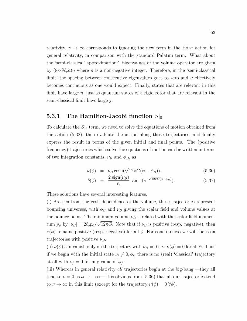
62

relativity, γ → ∞ corresponds to ignoring the new term in the Holst action for

general relativity, in comparison with the standard Palatini term. What about

the ‘semi-classical’ approximation? Eigenvalues of the volume operator are given

by (8πG`o~)n where n is a non-negative integer. Therefore, in the ‘semi-classical

limit’ the spacing between consecutive eigenvalues goes to zero and ν effectively

becomes continuous as one would expect. Finally, states that are relevant in this

limit have large n, just as quantum states of a rigid rotor that are relevant in the

semi-classical limit have large j.

5.3.1 The Hamilton-Jacobi function S|0To calculate the S|0 term, we need to solve the equations of motion obtained from

the action (5.32), then evaluate the action along those trajectories, and finally

express the result in terms of the given initial and final points. The (positive

frequency) trajectories which solve the equations of motion can be written in terms

of two integration constants, νB and φB, as

ν(φ) = νB cosh(√

12πG(φ− φB)), (5.36)

b(φ) =2 sign(νB)

`otan−1(e−

√12πG(φ−φB)). (5.37)

These solutions have several interesting features.

(i) As seen from the cosh dependence of the volume, these trajectories represent

bouncing universes, with φB and νB giving the scalar field and volume values at

the bounce point. The minimum volume νB is related with the scalar field momen-

tum pφ by |νB| = 2`opφ/√

12πG. Note that if νB is positive (resp. negative), then

ν(φ) remains positive (resp. negative) for all φ. For concreteness we will focus on

trajectories with positive νB.

(ii) ν(φ) can vanish only on the trajectory with νB = 0 i.e., ν(φ) = 0 for all φ. Thus

if we begin with the initial state νi 6= 0, φi, there is no (real) ‘classical’ trajectory

at all with νf = 0 for any value of φf .

(iii) Whereas in general relativity all trajectories begin at the big-bang —they all

tend to ν = 0 as φ→ −∞— it is obvious from (5.36) that all our trajectories tend

to ν →∞ in this limit (except for the trajectory ν(φ) = 0 ∀φ).

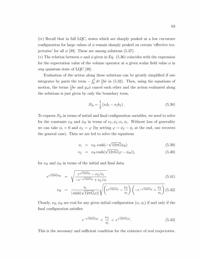
63

(iv) Recall that in full LQC, states which are sharply peaked at a low curvature

configuration for large values of φ remain sharply peaked on certain ‘effective tra-

jectories’ for all φ [39]. These are among solutions (5.37).

(v) The relation between ν and φ given in Eq. (5.36) coincides with the expression

for the expectation value of the volume operator at a given scalar field value φ in

any quantum state of LQC [38].

Evaluation of the action along these solutions can be greatly simplified if one

integrates by parts the term −∫ 1

0dτ 1

2bν in (5.32). Then, using the equations of

motion, the terms 12bν and pφφ cancel each other and the action evaluated along

the solutions is just given by only the boundary term,

S|0 =1

2(νibi − νfbf ) . (5.38)

To express S|0 in terms of initial and final configuration variables, we need to solve

for the constants νB and φB in terms of νf , φf ; νi, φi. Without loss of generality

we can take φi = 0 and φf = ϕ (by setting ϕ = φf − φi at the end, one recovers

the general case). Then we are led to solve the equations

νi = νB cosh(−√

12πGφB) (5.39)

νf = νB cosh(√

12πG(ϕ− φB)), (5.40)

for νB and φB in terms of the initial and final data:

e√

12πGφB =

√e√

12πGϕ − νf/νi−e−

√12πGϕ + νf/νi

(5.41)

νB =νi

| sinh(√

12πGϕ)|

√(e√

12πGϕ − νfνi

)(−e−

√12πGϕ +

νfνi

).(5.42)

Clearly, νB, φB are real for any given initial configuration (νi, φi) if and only if the

final configuration satisfies

e−√

12πG|ϕ| <νfνi

< e√

12πG|ϕ|. (5.43)

This is the necessary and sufficient condition for the existence of real trajectories.

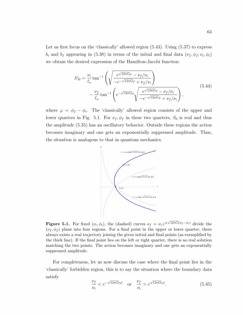
64

Let us first focus on the ‘classically’ allowed region (5.43). Using (5.37) to express

bi and bf appearing in (5.38) in terms of the initial and final data (νf , φf ; νi, φi)

we obtain the desired expression of the Hamilton-Jacobi function:

S|0 =νi`o

tan−1

(√e√

12πGϕ − νf/νi−e−

√12πGϕ + νf/νi

)

− νf`o

tan−1

(e−√

12πGϕ

√e√

12πGϕ − νf/νi−e−

√12πGϕ + νf/νi

),

(5.44)

where ϕ = φf − φi. The ‘classically’ allowed region consists of the upper and

lower quarters in Fig. 5.1. For νf , φf in these two quarters, S0 is real and thus

the amplitude (5.35) has an oscillatory behavior. Outside these regions the action

becomes imaginary and one gets an exponentially suppressed amplitude. Thus,

the situation is analogous to that in quantum mechanics.

HΝ f ,Φ f L

HΝi,ΦiL

Ν = Νi exp@ 12 ΠG HΦ-ΦiLD

Ν = Νi exp@- 12 ΠG HΦ-ΦiLD

Ν = Νb cosh@ 12 ΠG HΦ-ΦbLD

Ν

Φ

Figure 5.1. For fixed (νi, φi), the (dashed) curves νf = νi e±√

12πG(φf−φi) divide the(νf , φf ) plane into four regions. For a final point in the upper or lower quarter, therealways exists a real trajectory joining the given initial and final points (as exemplified bythe thick line). If the final point lies on the left or right quarter, there is no real solutionmatching the two points. The action becomes imaginary and one gets an exponentiallysuppressed amplitude.

For completeness, let us now discuss the case where the final point lies in the

‘classically’ forbidden region, this is to say the situation where the boundary data

satisfyνfνi< e−

√12πG|ϕ| or

νfνi> e

√12πG|ϕ|. (5.45)

65

For concreteness let νi be positive as in Fig.5.1 but now there is no restriction

on the sign of νf . To find extrema of the action that join the initial and final

configurations satisfying (5.45), we can follow the semi-classical procedure used to

calculate tunneling amplitudes in familiar systems and allow paths with imaginary

momenta. Let us define

b = ib, p = ip, α = iα, S = iS. (5.46)

Eq. (5.32) then implies

S =

∫dτ

(pφ− 1

2bν + α

(p2 − 3πGν2 sinh2 `ob

`2o

)). (5.47)

We now consider the case when the tilde quantities are real and compute the

stationary trajectories of S. The ‘positive frequency’ (i.e. p > 0) trajectories are

parameterized by two integrations constants, νo and φo, and take the form

ν(φ) = νo sinh(√

12πG(φ− φo)), (5.48)

b(φ) =2 sign(νo)

`otanh−1(e−

√12πG|φ−φo|). (5.49)

They represent universes that go through a singularity at φ = φo, where the

volume vanishes and b diverges. As in the ‘classically’ allowed region we have

|νo| = 2`op/√

12πG. In terms of the initial and final data, the integration constants

are

e√

12πGφo =

√e√

12πGϕ − νf/νie−√

12πGϕ − νf/νi(5.50)

νo =|νi| sign(νf − νi)sinh(

√12πGϕ)

√(e√

12πGϕ − νfνi

)(e−√

12πGϕ − νfνi

), (5.51)

which, as expected, take real values in the ‘forbidden’ region (5.45). The action

can then be evaluated as before. Although now the paths encounter a divergence

in b, the integral (5.47) is convergent and given by the tilde version of (5.38).

(Moreover, the product ν(φ)b(φ) is always finite and vanishes at φ = φo.) For the

66

case when ϕ > 0 and νf/νi < e−√

12πGϕ the result is

S|0 =νi`o

tanh−1

(√e−√

12πGϕ − νf/νie√

12πGϕ − νf/νi

)

− νf`o

tanh−1

(e√

12πGϕ

√e−√

12πGϕ − νf/νie√

12πGϕ − νf/νi

).

(5.52)

Similar expressions hold for other regions. For instance, in the ϕ > 0, νf/νi >

e√

12πGϕ case the action takes the same form, except that the arguments of the

tanh−1 functions are the reciprocals of the ones appearing in (5.52).

In all cases, S|0 is negative; the extraction amplitude is exponentially sup-

pressed for paths in the ‘classically forbidden’ regions. But as we approach the

dashed curves marking the boundary of the ‘classically’ allowed and forbidden re-

gions, the action S goes to zero. In particular then, from Fig.5.1 it may appear

that for any given νi there is a significant probability of reaching the singularity

νf = 0 for large ϕ = φf −φi. However, as is common in more familiar systems, the

steepest descent approximation also becomes poor in a neighborhood of the dashed

curves! Indeed, we know from full LQC that (in the deparameterized framework)

the expectation value of |ν| tends to infinity for large ϕ. More generally, plots of

the exact extraction amplitudes in Sec.5.3.3 will show that the amplitude is always

suppressed in the classically forbidden regions. Thus, while the steepest descent

approximation provides much physical insight, it is by no means a substitute for

the full quantum theory.

5.3.2 det δ2S|0 and the WKB approximation

To compute the amplitude (det δ2S|0)−1/2

, one would need a suitable regularization

in order to deal with the infinite dimensional determinant. This is can be done

in ordinary quantum mechanics or field theory, and should as well be doable here.

We will however take a different route and calculate this factor by means of the

WKB approximation [54, 55].

Note that the extraction amplitude A(νf , φf ; νi, φi) can be thought of as a

physical state if one takes the initial data as fixed parameters and the final data

67

as arguments of the wavefunction: the family of states

Ψνi,φi(νf , φf ) := A(νf , φf ; νi, φi), (5.53)

parameterized by νi and φi satisfy the constraint equation

C Ψνi,φi = 0. (5.54)

The ~ expansions underlying the desired WKB approximation are discussed in

Appendix 5.B. We begin with the ansatz for the physical state:

Ψνi,φi(νf , φf ) = a(νf , φf ; νi, φi) ei~ W (νf ,φf ;νi,φi) +O(~). (5.55)

Following the procedure of Appendix 5.B, the imposition of the constraint equation

(5.54) to zeroth and first order in ~ leads to the following equations for a and W :

C(νf , φf , ∂νfW,∂φfW ) = 0, and LX a = 0 (5.56)

where

C(ν, φ, b, pφ) = p2φ − 3πG

sin2 `ob

`2o

ν2

is the ‘effective constraint’, and

X =∂C

∂pφ

∣∣∣∣pφ=∂qfW

∂

∂qf

is the vector field on configuration space qf = (νf , φf ) obtained from the Hamilto-

nian vector field of the constraint.

The first equation is the Hamilton-Jacobi equation and, as expected, one can

check that S|0 given by (5.44) solves it. The amplitude a is determined by the

second equation together with the condition

a(νi, φi; νf , φf ) = a(νf , φf ; νi, φf ) (5.57)

68

which follows from the fact that Ψνi,φi(νf , φf ) = Ψνf ,φf (νi, φi):

a = |ν2i (e

√12πGϕ − νf

νi) (−e−

√12πGϕ +

νfνi

)|−1/4. (5.58)

This is the factor we identify with (det δ2S|0)−1/2

. Note that this quantity diverges

at νf = νie±√

12πGϕ (dashed lines in Fig. 5.1) where the amplitude goes from

oscillatory to exponential decay behavior. Thus, the WKB approximation can be

valid only away from the dashed lines. This simply mirrors what happens in the

WKB approximation in ordinary quantum mechanics.

To summarize, we have succeeded in finding a saddle point approximation of

the path integral as in equation (5.35). The determinant factor was not calculated

directly but by matching with the terms of a WKB expansion. Therefore, we will

call the resulting approximate extraction amplitude AWKB:

AWKB(νf , φf ; νi, φi) := a ei~S|0 , (5.59)

where a is given by Eq. (5.58), S|0 by Eq. (5.44) and as before ϕ = φf − φi. We

now proceed to numerically compare this approximate amplitude with the exact

one.

5.3.3 Comparison with exact solution

One of the advantages of the model under study is its solvability [38]. In partic-

ular, it is possible to obtain a closed form expression of the extraction amplitude

A(νf , φf ; νi, φi) [41]. This is displayed in Section 5.C. We calculated the exact so-

lution numerically and compared it with the saddle point approximation obtained

in Sec.5.3.2. We found that there is a good agreement away from the dashed lines

of Fig. 5.1 which mark the transition between the ‘classically’ allowed region to the

‘classically’ forbidden one. Along the dashed line, however, the WKB amplitude

diverges and the approximation fails badly just as in ordinary quantum mechanics.

We illustrate these results in figures 5.2, 5.3 and 5.4. In the first two figures we

plot of the real parts of the exact and WKB amplitudes as a function of νf and

φf respectively, for fixed values of the remaining variables. The exact amplitude

shows a sudden transition from oscillatory to decaying behavior. If one had access

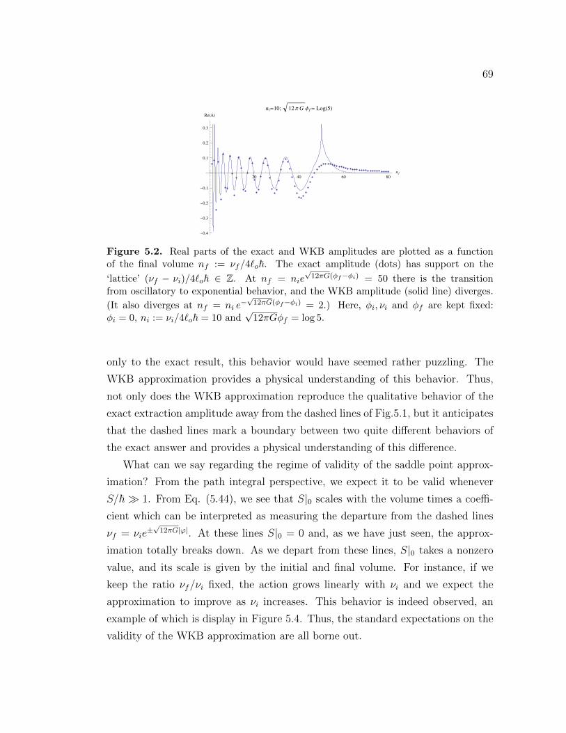
69

20 40 60 80

n f

-0.4

-0.3

-0.2

-0.1

0.1

0.2

0.3

ReHAL

ni=10; 12 ΠG Φ f= LogH5L

Figure 5.2. Real parts of the exact and WKB amplitudes are plotted as a functionof the final volume nf := νf/4`o~. The exact amplitude (dots) has support on the

‘lattice’ (νf − νi)/4`o~ ∈ Z. At nf = nie√

12πG(φf−φi) = 50 there is the transitionfrom oscillatory to exponential behavior, and the WKB amplitude (solid line) diverges.

(It also diverges at nf = ni e−√

12πG(φf−φi) = 2.) Here, φi, νi and φf are kept fixed:φi = 0, ni := νi/4`o~ = 10 and

√12πGφf = log 5.

only to the exact result, this behavior would have seemed rather puzzling. The

WKB approximation provides a physical understanding of this behavior. Thus,

not only does the WKB approximation reproduce the qualitative behavior of the

exact extraction amplitude away from the dashed lines of Fig.5.1, but it anticipates

that the dashed lines mark a boundary between two quite different behaviors of

the exact answer and provides a physical understanding of this difference.

What can we say regarding the regime of validity of the saddle point approx-

imation? From the path integral perspective, we expect it to be valid whenever

S/~ 1. From Eq. (5.44), we see that S|0 scales with the volume times a coeffi-

cient which can be interpreted as measuring the departure from the dashed lines

νf = νie±√

12πG|ϕ|. At these lines S|0 = 0 and, as we have just seen, the approx-

imation totally breaks down. As we depart from these lines, S|0 takes a nonzero

value, and its scale is given by the initial and final volume. For instance, if we

keep the ratio νf/νi fixed, the action grows linearly with νi and we expect the

approximation to improve as νi increases. This behavior is indeed observed, an

example of which is display in Figure 5.4. Thus, the standard expectations on the

validity of the WKB approximation are all borne out.

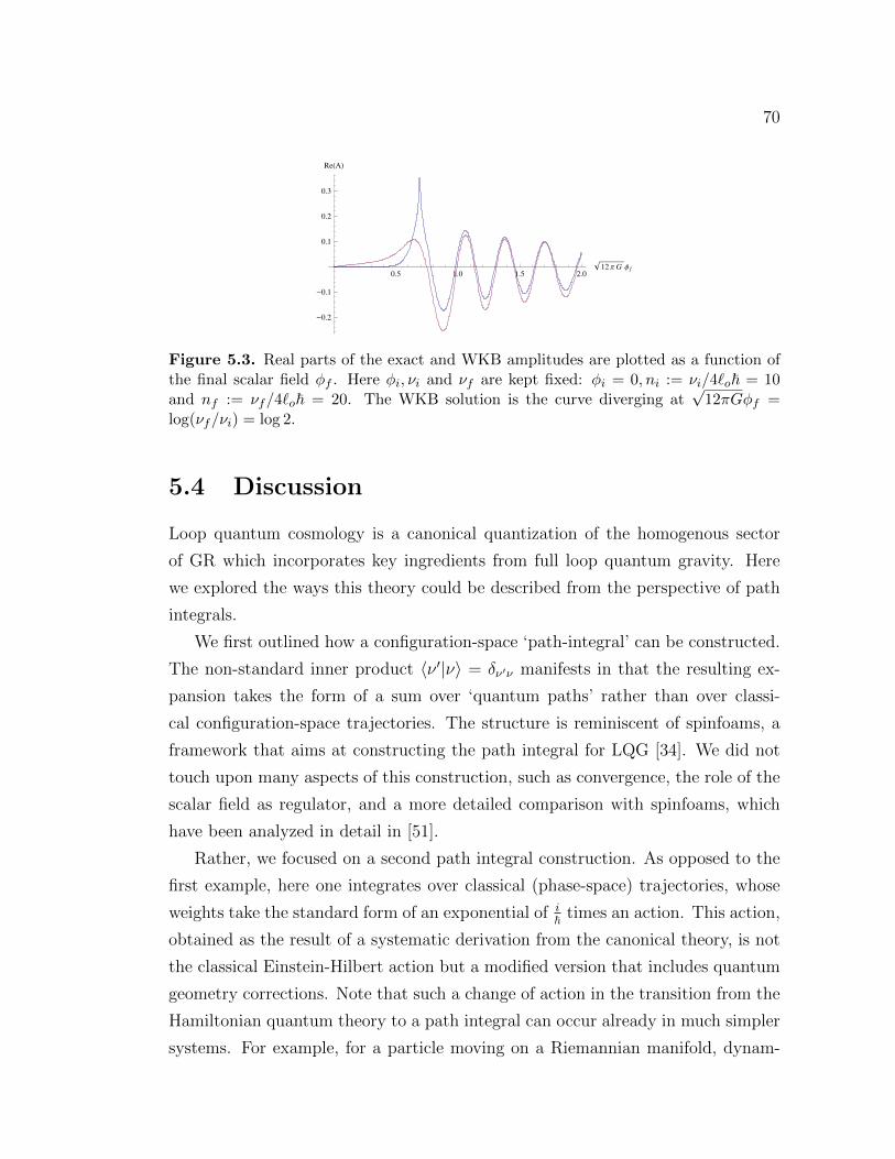
70

0.5 1.0 1.5 2.0

12 ΠG Φ f

-0.2

-0.1

0.1

0.2

0.3

ReHAL

Figure 5.3. Real parts of the exact and WKB amplitudes are plotted as a function ofthe final scalar field φf . Here φi, νi and νf are kept fixed: φi = 0, ni := νi/4`o~ = 10and nf := νf/4`o~ = 20. The WKB solution is the curve diverging at

√12πGφf =

log(νf/νi) = log 2.

5.4 Discussion

Loop quantum cosmology is a canonical quantization of the homogenous sector

of GR which incorporates key ingredients from full loop quantum gravity. Here

we explored the ways this theory could be described from the perspective of path

integrals.

We first outlined how a configuration-space ‘path-integral’ can be constructed.

The non-standard inner product 〈ν ′|ν〉 = δν′ν manifests in that the resulting ex-

pansion takes the form of a sum over ‘quantum paths’ rather than over classi-

cal configuration-space trajectories. The structure is reminiscent of spinfoams, a

framework that aims at constructing the path integral for LQG [34]. We did not

touch upon many aspects of this construction, such as convergence, the role of the

scalar field as regulator, and a more detailed comparison with spinfoams, which

have been analyzed in detail in [51].

Rather, we focused on a second path integral construction. As opposed to the

first example, here one integrates over classical (phase-space) trajectories, whose

weights take the standard form of an exponential of i~ times an action. This action,

obtained as the result of a systematic derivation from the canonical theory, is not

the classical Einstein-Hilbert action but a modified version that includes quantum

geometry corrections. Note that such a change of action in the transition from the

Hamiltonian quantum theory to a path integral can occur already in much simpler

systems. For example, for a particle moving on a Riemannian manifold, dynam-

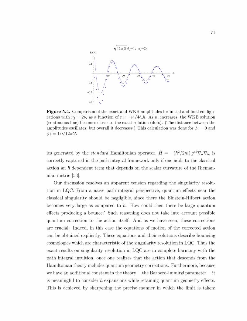
71

10 20 30 40 50

ni

-0.3

-0.2

-0.1

0.1

ReHAL

12 ΠG Φ f=1; n f=2ni

Figure 5.4. Comparison of the exact and WKB amplitudes for initial and final configu-rations with νf = 2νi as a function of ni := νi/4`o~. As ni increases, the WKB solution(continuous line) becomes closer to the exact solution (dots). (The distance between theamplitudes oscillates, but overall it decreases.) This calculation was done for φi = 0 andφf = 1/

√12πG.

ics generated by the standard Hamiltonian operator, H = −(~2/2m) gab∇a∇b, is

correctly captured in the path integral framework only if one adds to the classical

action an ~ dependent term that depends on the scalar curvature of the Rieman-

nian metric [53].

Our discussion resolves an apparent tension regarding the singularity resolu-

tion in LQC: From a naive path integral perspective, quantum effects near the

classical singularity should be negligible, since there the Einstein-Hilbert action

becomes very large as compared to ~. How could then there be large quantum

effects producing a bounce? Such reasoning does not take into account possible

quantum correction to the action itself. And as we have seen, these corrections

are crucial. Indeed, in this case the equations of motion of the corrected action

can be obtained explicitly. These equations and their solutions describe bouncing

cosmologies which are characteristic of the singularity resolution in LQC. Thus the

exact results on singularity resolution in LQC are in complete harmony with the

path integral intuition, once one realizes that the action that descends from the

Hamiltonian theory includes quantum geometry corrections. Furthermore, because

we have an additional constant in the theory —the Barbero-Immirzi parameter— it

is meaningful to consider ~ expansions while retaining quantum geometry effects.

This is achieved by sharpening the precise manner in which the limit is taken:

72

~ → 0, γ → ∞ such that ~γ3 = const. This ~ expansion enables us to introduce

the WKB approximation which helps one understand features of the exact ampli-

tude, e.g., the oscillatory versus damping behavior that occurs as one varies the

final configuration (νf , φf ) keeping the initial configuration (νi, φi) fixed. It also

provides an ‘explanation’ of the surprising effectiveness of the effective equations

[56] in LQC from a path integral framework.

Thus, from the LQC perspective, it would be incorrect to simply define the

theory starting with smooth metrics and matter fields and assigning to each path

the weight that comes from the Einstein Hilbert action because this procedure

completely ignores the quantum nature of the underlying Riemannian geometry.

For a satisfactory treatment of ultraviolet issues such as the singularity resolution,

it is crucial that the calculation retains appropriate memory of this quantum na-

ture. This viewpoint can be traced back to full LQG and spinfoam models. In

full LQG, quantum geometry is an essential feature already of kinematics. It is

then not surprising that in spinfoams the histories that one sums over are quantum

geometries. This situation is parallel to the configuration space path integral dis-

cussed in Section 5.1. In LQC we were fortunate in that the integral over quantum

paths could be recast into an integral over all paths in the classical phase space.

This enabled us to carry out the steepest descent approximation and develop phys-

ical intuition for the qualitative properties of the exact extraction amplitude. A

similar reformulation of spinfoams of the full theory appears to be difficult. But

if it could somehow be achieved, one would have a powerful tool both to probe

semi-classical aspects of full quantum gravity and to develop valuable intuition

for the ultraviolet properties of the theory. In particular, the resulting quantum

geometry corrections to the full Einstein-Hilbert action would bring the difference

between spin foams and perturbative path integrals into sharp focus.

5.A Appendix: Path integrals for polymerized

free particle

This appendix parallels the analysis of the chapter, but with the system under

study being a ‘polymerized’ free particle [45, 57]. In particular we will be dealing

73

with a true Hamiltonian and evolution operator rather than with a constraint

equation. Along the analysis of this model, we will prove some general results

that where used in the main body of the chapter. There will also be a difference

with the LQC analysis regarding the saddle point approximation, Section 5.A.3.

The simplicity of the model allow ones to directly compute the ~→ 0 asymptotics

of the transition amplitude by means of a standard, one-dimensional saddle point

approximation. Instead of reproducing the analysis we did in the LQC case, Section

5.3, we will directly evaluate the ~ → 0 limit and then verify the result is in

agreement with the expected one from path integrals.

Let us now specify the model. Starting with the classical free particle phase

space (x, p), we consider a ‘polymer’ quantization given by a Hilbert space of wave

functions ψ(x) with inner product,

||ψ||2 =∑x∈R

|ψ(x)|2. (5.60)

The classical Hamiltonian H = p2/2m has to be regularized in order to admit a

quantization on this Hilbert space. One possible regularization can be obtained

by introducing a momentum cutoff Λ and defining

HΛ :=Λ2

m[1− cos(

p

Λ)] = p2/2m+O(Λ−2). (5.61)

For fixed Λ, the resulting quantum theory corresponds to a particle on a lattice

aZ ⊂ R + ε, with a = ~/Λ and 0 ≤ ε < a. This is the system we will focus on.

One may argue whether such system should be regarded as a genuine ‘polymer’

system, since issues of non-separability of the Hilbert space can be sidestepped by

restricting oneself to independent lattices. We note however that the same property

holds for the LQC system we studied, and so it will suffice for our purposes. We

should also point out that, from the two path integrals –configuration and phase

space– it is the second one that makes heavily use of this lattice property. The

formulation of the first one is completely general, although the lattice property

does simplify the computations.

In the polymer Hilbert space given by (5.60), the Hamiltonian (5.61) has a

74

straightforward quantization given by

(HΛψ)(x) = Λ2/m

(ψ(x)− ψ(x+ a) + ψ(x− a)

2

), (5.62)

which can be thought of as a discretization of the standard operator −~2/(2m)∇2.

Our object of interest will be the transition amplitude, defined by the matrix

element of the evolution operator:

U(xf , xi; t) := 〈xf |e−i~ tHΛ|xi〉. (5.63)

Our objective is to find the path integral descriptions for this transition ampli-

tude, following the standard Feynman prescription. We will discuss two possible

path integrals, one in configuration space and the other one in phase space. The

first construction is general and holds for any discrete basis, not just for systems

on a lattice like the present one. On the other hand, the phase space path integral

does rely on the ability to restrict oneself to a lattice.

5.A.1 Configuration space path integral

The first step is to express the transition amplitude (5.63) as a composition of

infinitesimal evolutions. Dividing the total time t in N time intervals of length

ε = t/N , one has

U(xf , xi; t) =∑

xN−1,...,x1

〈xf |e−i~ εHΛ|xN−1〉〈xN−1|e−

i~ εHΛ |xN−2〉 ... 〈x1|e−

i~ εHΛ |xi〉

(5.64)

where we have first split the exponential intoN identical terms and then introduced

a decomposition of the identity operator at each intermediate time tn = nε, n =

1, 2, .., N−1. Equation (5.64) can be thought of as a sum over ‘discrete-time’ paths.

Notice that, even though initially each sum ranges over all reals, xn ∈ R, only

countably number of terms are non-vanishing, namely those where xn − xi ∈ aZ.

The next step in the standard path integral construction is to take the ‘con-

tinuum time’ limit, N → ∞, of the skeletonization. Here is where the difference

with the ordinary case comes into play, since we have sums over xn as opposed to

75

integrals.

The idea is to rearrange the sum (5.64) according to paths that are piece-

wise constant, with a given number of transitions. A path with M transitions

corresponds to a discrete-time path of the form,

(xM , . . . , xM ; xM−1, . . . , xM−1; . . . . . . ;

N2︷ ︸︸ ︷x1, . . . , x1; x0, . . . , x0︸ ︷︷ ︸

N1

) , (5.65)

where Nm denotes the time-step at which the m-th transition takes place. For

fixed N , all paths take this form, with 0 ≤M ≤ N . Thus, the total sum in (5.64)

can be reorganized as

∑xN−1,...,x1

=N∑

M=0

N−1∑NM=M

NM−1∑NM−1=M−1

. . .

N2−1∑N1=1

∑xM−1,...,x1

xm 6=xm+1

, (5.66)

where a path on the right hand side is labeled by its transition number M , the

‘transition times’ Nm, and the intermediate positions xM−1, . . . , x1, corresponding

to a discrete-time path of the form (5.66).

As shown in [42], this rearrangement allows one to take the N → ∞ limit,

where one obtains

U(xf , xi; t) =∞∑

M=0

∫t>tM>...>t1>0

dtM . . . dt1∑

xM−1,...,x1

xm 6=xm+1

A(xM , . . . , x0; tM , . . . , t1)

(5.67)

where the amplitude of each ‘continuous-time’ path is given by

A(xM , . . . , x0; tM , . . . , t1; ) = e−i~ (t−tM )HxMxM (− i

~HxMxM−1

) ×

. . . e−i~ (t2−t1)Hx1x1 (− i

~Hx1x0) e−

i~ t1Hx0x0 , (5.68)

where,

Hyx ≡ 〈y|HΛ|x〉. (5.69)

We now provide a proof of equation (5.67), which does not involve the ‘continuous-

time’ limiting procedure. Expression (5.67) is reminiscent of a perturbative expan-

76

sion, with the number of transitions playing the role of the order of the perturba-

tion. The transitions are being weighted by off-diagonal matrix elements Hyx with

y 6= x. This motivates to consider a splitting of the Hamiltonian into its diagonal

and off-diagonal parts:

HΛ = D + K, (5.70)

where the matrix elements of D and K are given by:

Dyx = Hxx δyx, Kyx =

Hyx y 6= x

0 y = x.(5.71)

We now consider expressing the evolution operator U(t) = e−i~ HΛt using pertur-

bation theory, with D playing the role of unperturbed Hamiltonian and K the

perturbation. Following the textbook procedure, we define the interaction Hamil-

tonian as

HI(t) := ei~ tD K e−

i~ tD. (5.72)

Then the evolution in the interaction picture is dictated by the operator

U(t) = ei~ tDe−

i~ tHΛ , satisfying

dU(t)

dt= − i

~HI(t)U(t) . (5.73)

The solution of this equation is given by a time-ordered exponential:

U(t) = T e−i~

∫ t0HI(t

′)dt′

=∞∑

M=0

∫ t0dtM

∫ tM0

dtM−1 . . .∫ t2

0dt1 [− i

~HI(tM)] ... [− i~HI(t1)] . (5.74)

Upon inserting a complete basis in between each product [HI(tm+1)][HI(tm)], one

recovers (5.67).

So far we have not referred to the particular form of the Hamiltonian (5.61),

and the result (5.67) is very general. In particular it applies to the Θ operator of

the LQC example, providing the proof of equations (5.9) and (5.10).

We now specialize to the polymer free particle case. The matrix elements of

77

the Hamiltonian (5.61) are given by

〈y|HΛ|x〉 =

Λ2

mif y = x

− Λ2

2mif y − x = ±a

0 otherwise

. (5.75)

Thus, the only non-trivial amplitudes are the ones given by sequences

(xM , . . . , xm, xm+1, . . . , x0) (5.76)

such that xm+1−xm = ±a. From the form of the matrix elements (5.75), it is easy

to verify that such amplitudes only depend on the total number of transitions M ,

and are given by

Apath with M transitions =

(iΛ2

2m~

)Me−

itΛ2

m~ . (5.77)

The sum over different paths in (5.67) is then given by a combinatorial factor that

we now compute. Let

n := (xf − xi)/a , (5.78)

with n ∈ Z (for otherwise the total amplitude is zero). The combinatorial factor is

given by the number of ways of going from 0 to n by ±1 transitions, with M total

transitions. Let M+ and M− be the number of +1 and −1 transitions respectively,

so that M = M+ + M− and n = M+ −M−. For concreteness let us take n ≥ 0.

The possible values M can take are then given by

M = 2M− + n , M− = 0, 1, . . . (5.79)

and the total number of paths with given M− is(MM−

). The remaining piece of

the total amplitude (5.67) is given by the time integrals. Since the amplitudes are

independent of the transitions time, this simply gives a tM

M !overall factor. Thus

78

(5.67) reduces to

U(xf , xi; t) = e−itΛ2

m~

∞∑M−=0

1

(M− + n)!M−!

(itΛ2

2m~

)2M−+n

. (5.80)

A Bessel function can be recognized in the sum, and the total amplitude is given

by

U(xf , xi; t) = i|n|e−itΛ2

m~ J|n|

(tΛ2

m~

)(5.81)

where we now wrote the final result for arbitrary sign of n = (xf −xi)/a. One can

verify that (5.81) satisfies the Schrodinger equation3 with respect to the Hamil-

tonian (5.61) with initial condition U(xi, xf ; 0) = δxixf , and so it represents the

correct expression for the matrix elements of the evolution operator U(t) = e−i~ HΛt.

This type of expansion shares some of the expected properties of spin foam-

type path integrals, where paths are given by sequences of spin-network, but at the

same time it is completely different from standard path integrals, where amplitudes

are weighted by the classical action. In particular, it does not seem to be suited

for semiclassical analysis. In the next section, we will see how, for the polymer

free particle model, it is possible to construct an alternative path integral of the

‘standard’ form, that among other things allows one to extract the semiclassical

approximation.

5.A.2 Phase space path integral

The special property that HΛ only involves shifts of constant lengths a, allows one

to restrict attention to a lattice aZ ⊂ R and thus work in the now separable Hilbert

space of sequences ψn ≡ ψ(an). This space admits a momentum basis given by

〈an|p〉 =einp/Λ√

2πΛ, (5.82)

with p ∈ (−πΛ, πΛ). Further simplification of this model, which is absent in the

LQC case, is that the Hamiltonian (5.61) is diagonal in this basis, and so the

3This follows from the property of the Bessel function: 2dJn/ds(s) + Jn+1(s)− Jn−1(s) = 0.

79

evolution operator can be written as

U(anf , ani; t) =1

2πΛ

∫ πΛ

−πΛ

dp ei(nf−ni)p/Λ−itΛ2

m~ (1−cos p/Λ). (5.83)

Let us now go back to the ‘discrete-time’ sum over paths (5.64), and use (5.83)

to express each of the ‘infinitesimal’ evolutions. The result is a ‘discrete-time’

phase-space path integral:4

U(xf , xi; t) = (2πΛ)−N∑

xN−1,...,x1

∫dpN . . . dp1e

i~SN , (5.84)

where xk ∈ aZ, p ∈ (−πΛ, πΛ), and

SN = εN−1∑k=0

(pkxk+1 − xk

ε− Λ2

m(1− cos

pkΛ

)

). (5.85)

This now resembles a more standard path integral, except for the fact that the

paths being integrated are not the standard ones. Similar situation occurs in the

construction of the path integral for a particle in a circle [58], where by means of

the identity

∑m∈Z

∫ 2π

0

dθ f(θ,m) eimθ =

∫ ∞−∞

dx

∫ ∞−∞

dθ f(θ, x) eixθ, (5.86)

which holds for any continuous f(θ, x) with a 2π period in θ, one can obtain the

usual paths. Applying this in (5.84), one obtains

U(xf , xi; t) = (2π)−N∫dxN−1 . . . , dx1

∫dpN . . . dp1e

i~SN , (5.87)

where the integrals are over all reals, except for the pN one that remains with

the original domain. The formal N → ∞ limit of expression (5.87) defines the

4Unlike the LQC case, we do not need to use small ε approximations, since |p〉 diagonalizesthe Hamiltonian, compare with equation (5.24).

80

standard phase space path integral:

U(xf , xi; t) = limN→∞

RHS of (5.87) =:

∫DxDp e

i~S, (5.88)

with

S =

∫ t

0

dt′(p x−HΛ), (5.89)

HΛ = Λ2

m(1 − cos p

Λ), and the integral is over phase space paths with fixed config-

uration endpoints xi and xf . Among other things, this path integral can be used

to obtain a formal ~ expansion, whose leading term is given by the saddle point

approximation:

U(xf , xi; t) ∼(det δ2S|cl

)−1/2ei~S|cl , (5.90)

where S|cl is the action evaluated along the trajectory extremizing the action with

initial and final configuration points fixed, and the prefactor (det δ2S|cl)−1/2

rep-

resents a formal infinite dimensional determinant.

We will now study the ~ → 0 behavior of the transition amplitude, directly

from expression (5.81), and verify it is given by the saddle point approximation

(5.90).

5.A.3 Saddle point approximation

The trajectories extremizing the action are those obeying the equations of motion

of the Hamiltonian HΛ. These are given by

p(t′) = constant

x(t′) = xi + Λm

sin(p/Λ) t′,(5.91)

and represent a particle moving at a velocity v = Λm

sin( pΛ

). For the saddle point

evaluation (5.90), we need to find the trajectory for given initial and final positions

xi and xf and total time t. This is given by (5.91) with p determined by

sin(p/Λ) =m

Λ

xf − xit

, (5.92)

81

which has real solutions provided that,∣∣∣∣xf − xit

∣∣∣∣ ≤ Λ

m. (5.93)

For strict inequality, there exist two trajectories, one with |p| < πΛ/2 and the

other one with |p| > πΛ/2 (only trajectories with |p| ≤ πΛ contribute since the

final value of p in the path integral has to be in this range, see Eq. (5.87)). The

action evaluated along these trajectories is

S+ = tΛ(v arcsin v/vmax +

√v2

max − v2 − vmax

), |p| < πΛ/2

S− = tΛ(v(π − arcsin v/vmax)−

√v2

max − v2 − vmax

), |p| > πΛ/2

(5.94)

where

v := (xf − x0)/t (5.95)

vmax := Λ/m. (5.96)

When |v| = Λ/m, the two solutions collapse to a single one. The region |v| > Λ/m

represents ‘classically forbidden’ configurations, which will correspond to expo-

nentially suppressed amplitudes. For |v| < Λ/m, the saddle point approximation

will then involve the two terms (5.94). Each term will contain the (det δ2S|cl)−1/2

pre-factor, wich can be calculated by the WKB method as we did in Section 5.3.

Instead of repeating that procedure, we will now directly compute the ~ → 0

asymptotics of U(xi, xf ; t) and verify it reproduces the expected saddle point/WKB

approximation. To this end, we start by the integral representation (5.83). Defin-

ing

z := e−ip/Λ (5.97)

s :=tΛ2

m~= tΛvmax/~ (5.98)

we obtain the following contour integral representation,

U(xf , xi; t) =e−is

2πi

∮z−(n+1)ei

s2

(z+z−1)dz, (5.99)

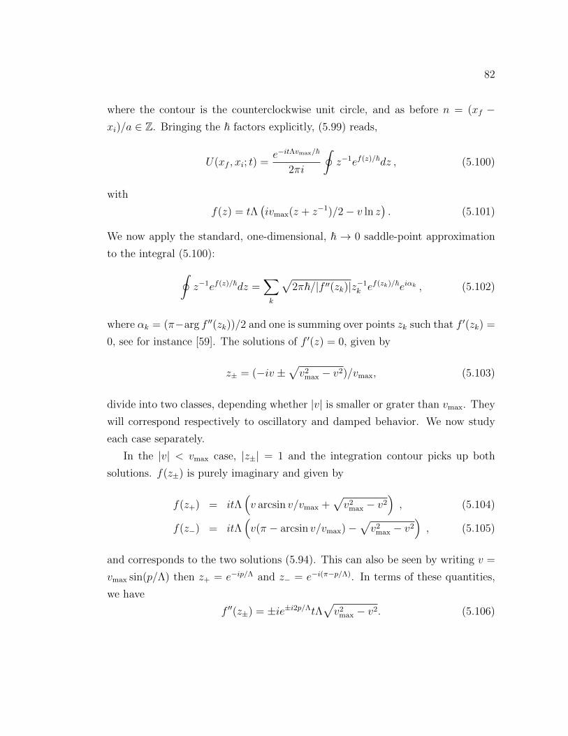
82

where the contour is the counterclockwise unit circle, and as before n = (xf −xi)/a ∈ Z. Bringing the ~ factors explicitly, (5.99) reads,

U(xf , xi; t) =e−itΛvmax/~

2πi

∮z−1ef(z)/~dz , (5.100)

with

f(z) = tΛ(ivmax(z + z−1)/2− v ln z

). (5.101)

We now apply the standard, one-dimensional, ~ → 0 saddle-point approximation

to the integral (5.100):∮z−1ef(z)/~dz =

∑k

√2π~/|f ′′(zk)|z−1

k ef(zk)/~eiαk , (5.102)

where αk = (π−arg f ′′(zk))/2 and one is summing over points zk such that f ′(zk) =

0, see for instance [59]. The solutions of f ′(z) = 0, given by

z± = (−iv ±√v2

max − v2)/vmax, (5.103)

divide into two classes, depending whether |v| is smaller or grater than vmax. They

will correspond respectively to oscillatory and damped behavior. We now study

each case separately.

In the |v| < vmax case, |z±| = 1 and the integration contour picks up both

solutions. f(z±) is purely imaginary and given by

f(z+) = itΛ(v arcsin v/vmax +

√v2

max − v2), (5.104)

f(z−) = itΛ(v(π − arcsin v/vmax)−

√v2

max − v2), (5.105)

and corresponds to the two solutions (5.94). This can also be seen by writing v =

vmax sin(p/Λ) then z+ = e−ip/Λ and z− = e−i(π−p/Λ). In terms of these quantities,

we have

f ′′(z±) = ±ie±i2p/ΛtΛ√v2

max − v2. (5.106)

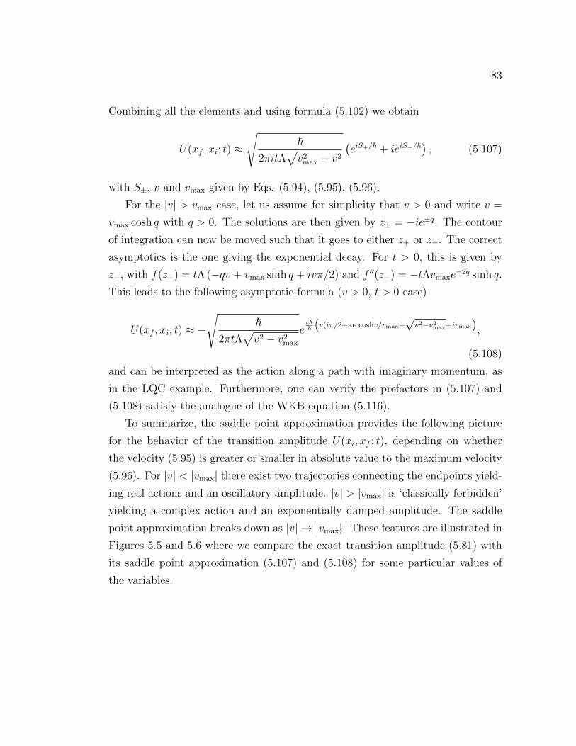
83

Combining all the elements and using formula (5.102) we obtain

U(xf , xi; t) ≈√

~2πitΛ

√v2

max − v2

(eiS+/~ + ieiS−/~

), (5.107)

with S±, v and vmax given by Eqs. (5.94), (5.95), (5.96).

For the |v| > vmax case, let us assume for simplicity that v > 0 and write v =

vmax cosh q with q > 0. The solutions are then given by z± = −ie±q. The contour

of integration can now be moved such that it goes to either z+ or z−. The correct

asymptotics is the one giving the exponential decay. For t > 0, this is given by

z−, with f(z−) = tΛ (−qv + vmax sinh q + ivπ/2) and f ′′(z−) = −tΛvmaxe−2q sinh q.

This leads to the following asymptotic formula (v > 0, t > 0 case)

U(xf , xi; t) ≈ −√

~2πtΛ

√v2 − v2

max

etΛ~

(v(iπ/2−arccoshv/vmax+

√v2−v2

max−ivmax

),

(5.108)

and can be interpreted as the action along a path with imaginary momentum, as

in the LQC example. Furthermore, one can verify the prefactors in (5.107) and

(5.108) satisfy the analogue of the WKB equation (5.116).

To summarize, the saddle point approximation provides the following picture

for the behavior of the transition amplitude U(xi, xf ; t), depending on whether

the velocity (5.95) is greater or smaller in absolute value to the maximum velocity

(5.96). For |v| < |vmax| there exist two trajectories connecting the endpoints yield-

ing real actions and an oscillatory amplitude. |v| > |vmax| is ‘classically forbidden’

yielding a complex action and an exponentially damped amplitude. The saddle

point approximation breaks down as |v| → |vmax|. These features are illustrated in

Figures 5.5 and 5.6 where we compare the exact transition amplitude (5.81) with

its saddle point approximation (5.107) and (5.108) for some particular values of

the variables.

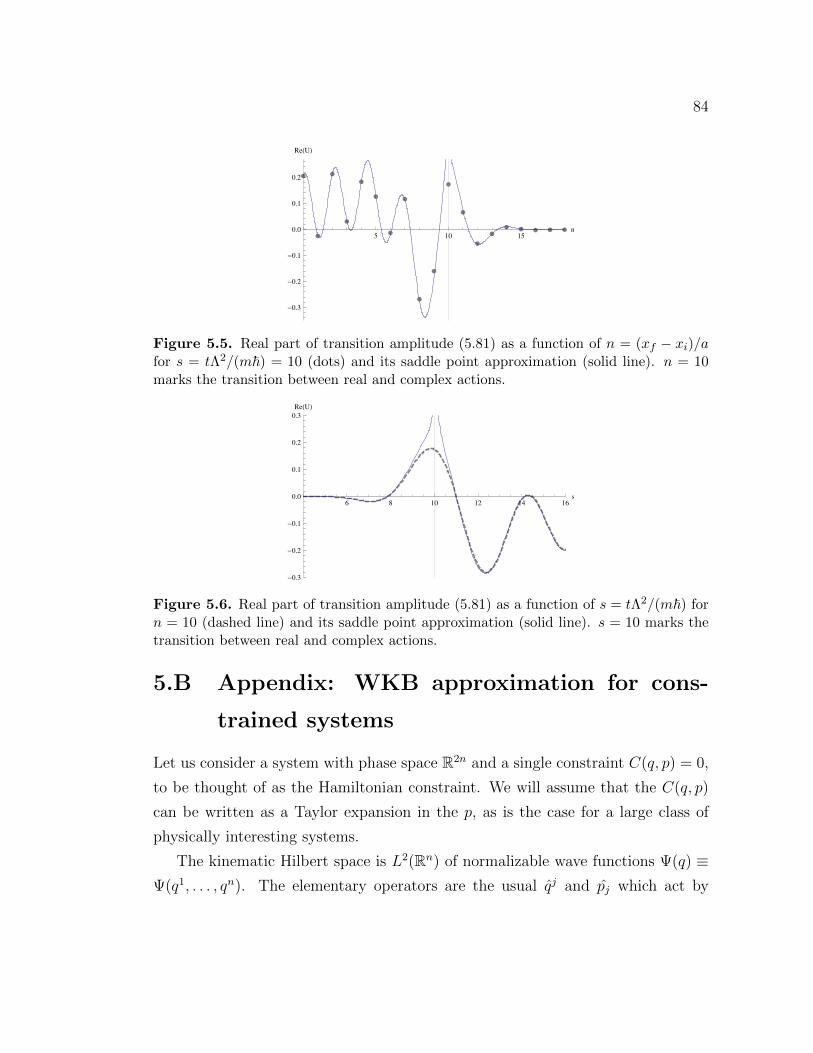
84

æ

æ

æ

æ

æ

æ

æ

æ

æ

æ

æ

æ

æ

æ

æ æ æ æ æ

5 10 15

n

-0.3

-0.2

-0.1

0.0

0.1

0.2

ReHUL

Figure 5.5. Real part of transition amplitude (5.81) as a function of n = (xf − xi)/afor s = tΛ2/(m~) = 10 (dots) and its saddle point approximation (solid line). n = 10marks the transition between real and complex actions.

6 8 10 12 14 16

s

-0.3

-0.2

-0.1

0.0

0.1

0.2

0.3

ReHUL

Figure 5.6. Real part of transition amplitude (5.81) as a function of s = tΛ2/(m~) forn = 10 (dashed line) and its saddle point approximation (solid line). s = 10 marks thetransition between real and complex actions.

5.B Appendix: WKB approximation for cons-

trained systems

Let us consider a system with phase space R2n and a single constraint C(q, p) = 0,

to be thought of as the Hamiltonian constraint. We will assume that the C(q, p)

can be written as a Taylor expansion in the p, as is the case for a large class of

physically interesting systems.

The kinematic Hilbert space is L2(Rn) of normalizable wave functions Ψ(q) ≡Ψ(q1, . . . , qn). The elementary operators are the usual qj and pj which act by

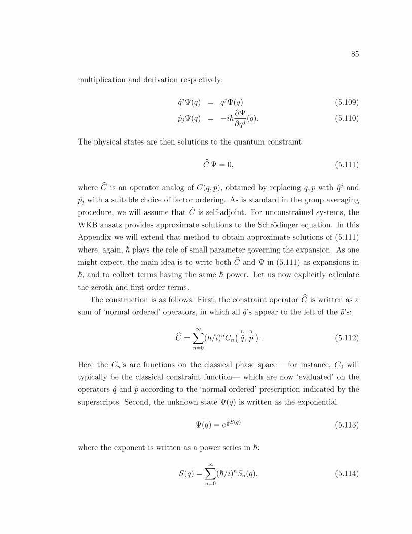
85

multiplication and derivation respectively:

qjΨ(q) = qjΨ(q) (5.109)

pjΨ(q) = −i~∂Ψ

∂qj(q). (5.110)

The physical states are then solutions to the quantum constraint:

C Ψ = 0, (5.111)

where C is an operator analog of C(q, p), obtained by replacing q, p with qj and

pj with a suitable choice of factor ordering. As is standard in the group averaging

procedure, we will assume that C is self-adjoint. For unconstrained systems, the

WKB ansatz provides approximate solutions to the Schrodinger equation. In this

Appendix we will extend that method to obtain approximate solutions of (5.111)

where, again, ~ plays the role of small parameter governing the expansion. As one

might expect, the main idea is to write both C and Ψ in (5.111) as expansions in

~, and to collect terms having the same ~ power. Let us now explicitly calculate

the zeroth and first order terms.

The construction is as follows. First, the constraint operator C is written as a

sum of ‘normal ordered’ operators, in which all q’s appear to the left of the p’s:

C =∞∑n=0

(~/i)nCn( L

q,R

p). (5.112)

Here the Cn’s are functions on the classical phase space —for instance, C0 will

typically be the classical constraint function— which are now ‘evaluated’ on the

operators q and p according to the ‘normal ordered’ prescription indicated by the

superscripts. Second, the unknown state Ψ(q) is written as the exponential

Ψ(q) = ei~S(q) (5.113)

where the exponent is written as a power series in ~:

S(q) =∞∑n=0

(~/i)nSn(q). (5.114)

86

Since C(q, p) is assumed to admit a Taylor expansion in the p, so do Cn(q, p).

Imposition of the quantum constraint (5.111) now leads to the following zeroth

and first order equations:

C0(q, ∂qS0) = 0, (5.115)

1

2

∂2C0

∂pi∂pj

∣∣∣∣p=∂qS0

∂2S0

∂qi∂qj+∂C0

∂pi

∣∣∣∣p=∂qS0

∂S1

∂qi+ C1(q, ∂qS0) = 0 (5.116)

The zeroth order equation (5.115) can be recognized as the Hamilton-Jacobi equa-

tion. The first order one, (5.116), can be rewritten as follows. If we use the fact

that C is self-adjoint, the condition C† = C, when applied to (5.112) implies

C1 =1

2

∂2C0

∂qj∂pj. (5.117)

Using (5.117), and writing a(q) := eS1(q), Eq. (5.116) can be written as a derivative

of the function a along the vector field

X :=∂C0

∂pj

∣∣∣∣p=∂qS0

∂

∂qj(5.118)

as

X(a) +1

2a divX = 0. (5.119)

The divergence term in (5.119) suggest one to interpret a and Ψ ∼ a ei~S0 as

half densities on Rn. Then (5.119) is just the Lie derivative of a along X:

Eq. (5.116) ⇐⇒ LXa = 0. (5.120)

These are the equations used in Sec. 5.3.2.

5.C Appendix: Exact Amplitude

In Sec.5.3.3 we compared the exact extraction amplitude with the WKB approxi-

mation. In this Appendix we recall from [41] the expression that was used in the

numerical evaluation of the exact amplitude.

The first step in the calculation is to find the eigenvectors of Θ. They are given

87

by |k±〉, with k > 0, satisfying the eigenvalue equation

Θ|k±〉 = 12πGk2~2|k±〉. (5.121)

These vectors are not normalized; the decomposition of the identity reads

I =∫∞

0dk

2πk sinh(πk)(|k+〉〈k + | + |k−〉〈k − |) . (5.122)

In terms of the ‘volume basis’ |4n`o~〉 used in the main body of this paper, the

vectors |k±〉 are given by

〈4n`o~|k±〉 =

√4|n|πikP±n(k) ±n ≥ 0

0 ±n < 0, (5.123)

where Pn(k) is the following (2n− 1)-degree polynomial in k:

Pn(k) :=1

ik(2n)!

d2n

ds2n

∣∣∣∣s=0

(1− s1 + s

)ik=

2n∑m=0

1

m!(2n−m)!

2n−1∏l=1

(ik+m−l). (5.124)

We are now ready to present the expression of the extraction amplitude. For

this, it is convenient to work in the deparameterized framework. In [41] it was

shown that the extraction amplitude in the timeless framework coincides with the

transition amplitude of the deparameterized theory:5

A(νf , φf ; νi, φi) = 〈νf | ei~√

Θ (φf−φi) |νi〉. (5.125)

Let us take νi = 4`o~ni and νf = 4`o~nf with ni and nf positive integers, and

define t :=√

12πG(φf − φi).By inserting the complete basis (5.122) in the right hand side of (5.125), we

5Equality (5.125) holds for the extraction amplitude with a normalization given by

A+(νf , φf ; νi, φi) = (2∫

dα 〈νf , φf | eiαC |pφ| |νi, φi〉 )+, and where one further selects the posi-tive pφ part (indicated by the +).

88

obtain

A(νf , φf ; νi, φi) = −2√ninf

∫∞0

dksinh(πk)

Pnf (k)Pni(k) keikt (5.126)

= −2√ninf Pnf (−i∂t)Pni(−i∂t)

∫∞0

dksinh(πk)

keikt (5.127)

= −√ninf

π2Pnf (−i∂t)Pni(−i∂t)ψ(1)(1/2− i t

2π) (5.128)

where ψ(1)(z) = d log Γ(z)/dz, and Γ(z) = (z − 1)! is the Gamma function.

This last expression (5.128) was the one used to numerically compute the exact

extraction amplitude for the plots in Sec. 5.3.3.

Bibliography

[1] Wald, R. (1984) General Relativity, University of Chicago Press.

[2] Kokkotas, K. D. and B. Schmidt (1999) “Quasi-Normal Modes of Starsand Black Holes,” Living Reviews in Relativity, 2(2).

[3] Pretorius, F. (2007) “Binary Black Hole Coalescence,” 0710.1338.

[4] Centrella, J., J. G. Baker, B. J. Kelly, and J. R. van Meter (2010)“Black-hole binaries, gravitational waves, and numerical relativity,” Rev. Mod.Phys., 82, pp. 3069–3119.

[5] Ashtekar, A. and B. Krishnan (2004) “Isolated and dynamical horizonsand their applications,” Living Rev.Rel., 7, p. 10, gr-qc/0407042.

[6] Buonanno, A., G. B. Cook, and F. Pretorius (2007) “Inspiral, mergerand ring-down of equal-mass black-hole binaries,” Phys.Rev., D75, p. 124018,gr-qc/0610122.

[7] Schnetter, E., B. Krishnan, and F. Beyer (2006) “Introduction todynamical horizons in numerical relativity,” Phys.Rev., D74, p. 024028,gr-qc/0604015.

[8] Owen, R. (2009) “The Final Remnant of Binary Black Hole Mergers: Mul-tipolar Analysis,” Phys.Rev., D80, p. 084012, 0907.0280.

[9] Poisson, E. (2004) A Relativist’s Toolkit: The Mathematics of Black-HoleMechanics, Cambridge University Press.

[10] Kuroda, Y. (1984) “Naked Singularities in the Vaidya Spacetimee,” Prog.Theor. Phys., 72, pp. 63–72.

[11] Booth, I. (2005) “Black hole boundaries,” Can.J.Phys., 83, pp. 1073–1099,gr-qc/0508107.

90

[12] Ashtekar, A., J. Engle, T. Pawlowski, and C. Van Den Broeck(2004) “Multipole moments of isolated horizons,” Class.Quant.Grav., 21, pp.2549–2570, gr-qc/0401114.

[13] Bentivegna, E. (2008) Ringing in unison: exploring black hole coalescencewith quasinormal modes, Ph.D. thesis, Penn State University.URL https://etda.libraries.psu.edu/paper/8245/

[14] Jaramillo, J., R. Macedo, P. Moesta, and L. Rezzolla (2011) “To-wards a cross-correlation approach to strong-field dynamics in Black Holespacetimes,” AIP Conf.Proc., 1458, pp. 158–173, 1205.3902.

[15] Booth, I. and S. Fairhurst (2007) “Isolated, slowly evolving, and dynam-ical trapping horizons: Geometry and mechanics from surface deformations,”Phys.Rev., D75, p. 084019, gr-qc/0610032.

[16] Ashtekar, A., C. Beetle, and J. Lewandowski (2002) “Geome-try of generic isolated horizons,” Class.Quant.Grav., 19, pp. 1195–1225,gr-qc/0111067.

[17] Ashtekar, A. and B. Krishnan (2003) “Dynamical horizons and theirproperties,” Phys.Rev., D68, p. 104030, gr-qc/0308033.

[18] Fabbri, A. and J. Navarro-Salas (2005) Modeling Black Hole Evapora-tion, Imperial College Press.

[19] Wald, R. (1994) Quantum Field Theory in Curved Spacetime and Black HoleThermodynamics, Chicago Lectures in Physics, University of Chicago Press.

[20] Ashtekar, A., C. Beetle, and J. Lewandowski (2001) “Mechanics ofrotating isolated horizons,” Phys.Rev., D64, p. 044016, gr-qc/0103026.

[21] Ashtekar, A., J. C. Baez, and K. Krasnov (2000) “Quantum geometryof isolated horizons and black hole entropy,” Adv.Theor.Math.Phys., 4, pp.1–94, gr-qc/0005126.

[22] Lewandowski, J. and T. Pawlowski (2003) “Extremal isolated hori-zons: A Local uniqueness theorem,” Class.Quant.Grav., 20, pp. 587–606,gr-qc/0208032.

[23] Gourgoulhon, E. (2007) “3+1 formalism and bases of numerical relativ-ity,” gr-qc/0703035.

[24] Owen, R., J. Brink, Y. Chen, J. D. Kaplan, G. Lovelace, et al.(2011) “Frame-Dragging Vortexes and Tidal Tendexes Attached to CollidingBlack Holes: Visualizing the Curvature of Spacetime,” Phys.Rev.Lett., 106,p. 151101, 1012.4869.

91

[25] Nichols, D. A., R. Owen, F. Zhang, A. Zimmerman, J. Brink, et al.(2011) “Visualizing Spacetime Curvature via Frame-Drag Vortexes and TidalTendexes I. General Theory and Weak-Gravity Applications,” Phys.Rev.,D84, p. 124014, 1108.5486.

[26] Lewandowski, J. and T. Pawlowski (2002) “Geometric characteriza-tions of the Kerr isolated horizon,” Int.J.Mod.Phys., D11, pp. 739–746,gr-qc/0101008.

[27] Gundlach, C. and J. M. Martn-Garca (2007) “Critical Phenomena inGravitational Collapse,” Living Reviews in Relativity, 10(5).

[28] Price, R. H., G. Khanna, and S. A. Hughes (2011) “Systematics of blackhole binary inspiral kicks and the slowness approximation,” Phys.Rev., D83,p. 124002, 1104.0387.

[29] Bartnik, R. and J. Isenberg (2006) “Spherically symmetric dynamicalhorizons,” Class.Quant.Grav., 23, pp. 2559–2570, gr-qc/0512091.

[30] Nakahara, M. (2003) Geometry, Topology and Physics, Second Edition,Graduate Student Series in Physics, Taylor & Francis.

[31] Bojowald, M. (2008) “Loop Quantum Cosmology,” Living Reviews in Rel-ativity, 11(4).

[32] Ashtekar, A. and P. Singh (2011) “Loop Quantum Cosmology: A StatusReport,” Class.Quant.Grav., 28, p. 213001, 1108.0893.

[33] Ashtekar, A. and J. Lewandowski (2004) “Background independentquantum gravity: a status report,” Classical and Quantum Gravity, 21, p. 53,arXiv:gr-qc/0404018.

[34] Perez, A. (2004) “Introduction to Loop Quantum Gravity and Spin Foams,”gr-qc/0409061.

[35] Ashtekar, A., M. Bojowald, and J. Lewandowski (2003) “Mathemati-cal structure of loop quantum cosmology,” Adv.Theor.Math.Phys., 7, pp. 233–268, gr-qc/0304074.

[36] Lewandowski, J., A. Okolow, H. Sahlmann, and T. Thiemann (2006)“Uniqueness of diffeomorphism invariant states on holonomy-flux algebras,”Commun.Math.Phys., 267, pp. 703–733, gr-qc/0504147.

[37] Fleischhack, C. (2009) “Representations of the Weyl Algebra in Quan-tum Geometry,” Communications in Mathematical Physics, 285, pp. 67–140,arXiv:math-ph/0407006.

92

[38] Ashtekar, A., A. Corichi, and P. Singh (2008) “Robustness of key fea-tures of loop quantum cosmology,” Phys.Rev., D77, p. 024046, 0710.3565.

[39] Ashtekar, A., T. Pawlowski, and P. Singh (2006) “Quantum Na-ture of the Big Bang: Improved dynamics,” Phys.Rev., D74, p. 084003,gr-qc/0607039.

[40] Marolf, D. (1995) “Refined algebraic quantization: Systems with a singleconstraint,” gr-qc/9508015.

[41] Ashtekar, A., M. Campiglia, and A. Henderson (2010) “Casting LoopQuantum Cosmology in the Spin Foam Paradigm,” Class.Quant.Grav., 27, p.135020, 1001.5147.

[42] ——— (2009) “Loop Quantum Cosmology and Spin Foams,” Phys.Lett.,B681, pp. 347–352, 0909.4221.

[43] Ashtekar, A. (2008) “Loop Quantum Gravity:. Four Recent Advances anda Dozen Frequently Asked Questions,” in The Eleventh Marcel GrossmannMeeting On Recent Developments in Theoretical and Experimental GeneralRelativity, Gravitation and Relativistic Field Theories (H. Kleinert, R. T.Jantzen, and R. Ruffini, eds.), pp. 126–147, 0705.2222.

[44] Simon, B. (1971) “Topics in Functional Analysis,” in Mathematics of Con-temporary Physics (R. F. Streater, ed.), Academic Press, London.

[45] Ashtekar, A., S. Fairhurst, and J. L. Willis (2003) “Quantum gravity,shadow states, and quantum mechanics,” Class.Quant.Grav., 20, pp. 1031–1062, gr-qc/0207106.

[46] Feynman, R. and A. Hibbs (1965) Quantum mechanics and path integrals,International series in pure and applied physics, McGraw-Hill.

[47] Feynman, R. (1948) “Space-time approach to nonrelativistic quantum me-chanics,” Rev.Mod.Phys., 20, pp. 367–387.

[48] Hartle, J. B. and K. V. Kuchar (1986) “Path integrals in parametrizedtheories: The free relativistic particle,” Phys. Rev. D, 34, pp. 2323–2331.

[49] Halliwell, J. J. (1988) “Derivation of the Wheeler-DeWitt equation froma path integral for minisuperspace models,” Phys. Rev. D, 38, pp. 2468–2481.

[50] Marolf, D. (1996) “Path integrals and instantons in quantum gravity: Min-isuperspace models,” Phys.Rev., D53, pp. 6979–6990, gr-qc/9602019.

93

[51] Henderson, A. (2011) Loop Quantum Cosmology: A Window Into the PathIntegral Representation of Quantum Gravity, Ph.D. thesis, Penn State Uni-versity.URL https://etda.libraries.psu.edu/paper/12472/

[52] Reisenberger, M. P. and C. Rovelli (1997) “’Sum over surfaces’ form ofloop quantum gravity,” Phys.Rev., D56, pp. 3490–3508, gr-qc/9612035.

[53] DeWitt, B. S. (1957) “Dynamical theory in curved spaces. 1. A Review ofthe classical and quantum action principles,” Rev.Mod.Phys., 29, pp. 377–397.

[54] Guillemin, V. and S. Sternberg (1977) Geometric asymptotics, Mathe-matical surveys, American Mathematical Society.

[55] Bates, S. and A. Weinstein (1997) Lectures on the Geometry of Quantiza-tion, Berkeley Mathematics Lecture Notes, American Mathematical Society.

[56] Taveras, V. (2008) “Corrections to the Friedmann Equations from LQG fora Universe with a Free Scalar Field,” Phys.Rev., D78, p. 064072, 0807.3325.

[57] Corichi, A., T. Vukasinac, and J. A. Zapata (2007) “Polymer QuantumMechanics and its Continuum Limit,” Phys.Rev., D76, p. 044016, 0704.0007.

[58] Kleinert, H. (2009) Path Integrals in Quantum Mechanics, Statistics, Poly-mer Physics, and Financial Markets, World Scientific.

[59] Arfken, G. and H. Weber (2005) Mathematical Methods for Physicists,Elsevier.

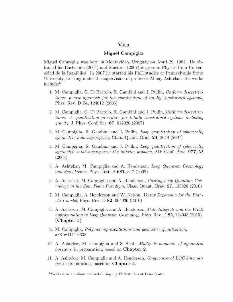
Vita

Miguel Campiglia

Miguel Campiglia was born in Montevideo, Uruguay on April 29, 1982. He ob-tained his Bachelor’s (2004) and Master’s (2007) degrees in Physics from Univer-sidad de la Republica. In 2007 he started his PhD studies at Pennsylvania StateUniversity, working under the supervision of professor Abhay Ashtekar. His worksinclude:6

1. M. Campiglia, C. Di Bartolo, R. Gambini and J. Pullin, Uniform discretiza-tions: a new approach for the quantization of totally constrained systems,Phys. Rev. D 74, 124012 (2006)

2. M. Campiglia, C. Di Bartolo, R. Gambini and J. Pullin, Uniform discretiza-tions: A quantization procedure for totally constrained systems includinggravity, J. Phys. Conf. Ser. 67, 012020 (2007)

3. M. Campiglia, R. Gambini and J. Pullin, Loop quantization of sphericallysymmetric midi-superspaces, Class. Quant. Grav. 24, 3649 (2007)

4. M. Campiglia, R. Gambini and J. Pullin, Loop quantization of sphericallysymmetric midi-superspaces: the interior problem, AIP Conf. Proc. 977, 52(2008)

5. A. Ashtekar, M. Campiglia and A. Henderson, Loop Quantum Cosmologyand Spin Foams, Phys. Lett. B 681, 347 (2009)

6. A. Ashtekar, M. Campiglia and A. Henderson, Casting Loop Quantum Cos-mology in the Spin Foam Paradigm, Class. Quant. Grav. 27, 135020 (2010)

7. M. Campiglia, A. Henderson and W. Nelson, Vertex Expansion for the Bian-chi I model, Phys. Rev. D 82, 064036 (2010)

8. A. Ashtekar, M. Campiglia and A. Henderson, Path Integrals and the WKBapproximation in Loop Quantum Cosmology, Phys. Rev. D 82, 124043 (2010).(Chapter 5)

9. M. Campiglia, Polymer representations and geometric quantization,arXiv:1111.0638

10. A. Ashtekar, M. Campiglia and S. Shah, Multipole moments of dynamicalhorizons, in preparation, based on Chapter 2.

11. A. Ashtekar, M. Campiglia and A. Henderson, Uniqueness of LQC kinemat-ics, in preparation, based on Chapter 4.

6Works 4 to 11 where realized during my PhD studies at Penn State.