The Pennsylvania State University

The Graduate School

LOW-WAVENUMBER TURBULENT BOUNDARY LAYER

WALL-PRESSURE MEASUREMENTS FROM VIBRATION DATA

OVER SMOOTH AND ROUGH SURFACES IN PIPE FLOW

A Thesis in

Acoustics

by

Neal D. Evans

c© 2011 Neal D. Evans

Submitted in Partial Fulfillment

of the Requirements

for the Degree of

Master of Science

August 2011

The thesis of Neal D. Evans was reviewed and approved∗ by the following:

Dean E. Capone

Associate Professor of Acoustics and Senior Research Associate

Thesis Advisor

William K. Bonness

Research Associate

Timothy A. Brungart

Associate Professor of Acoustics and Senior Research Associate

Victor W. Sparrow

Professor of Acoustics

Interim Chair, Graduate Program in Acoustics

∗Signatures are on file in the Graduate School.

Abstract

The vibration response of a thin cylindrical shell excited by fully-developed tur-bulent pipe flow is measured and used to extract the fluctuating pressure levelsgenerated by the boundary layer. Parameters used to extract the turbulent flowpressure levels are determined via experimental modal analyses of the water-filledpipe and measured vibration levels from flow through the pipe at 5.8 m/s. Mea-surements are reported for hydraulically smooth and fully rough surface conditions.Smooth wall-pressure levels are compared to the turbulent boundary layer pressuremodel of Chase (1987) and the measurements of Bonness, et al. (2010). Resultsfor the smooth pipe match the predicted smooth wall-pressure spectrum and cor-respond to a normalized low-wavenumber-white level of -41 dB. Pressure levelsfrom the fully rough condition display a low-wavenumber-white level of -28 dBfor a surface with uniformly distributed roughness elements, suggesting a 13 dBcorrection factor for a fully rough surface over a hydraulically smooth surface.

iii

Table of Contents

List of Figures vi

List of Tables viii

List of Symbols ix

Acknowledgments xi

Chapter 1Background 11.1 Introduction . . . . . . . . . . . . . . . . . . . . . . . . . . . . . . . 1

1.1.1 Motivation . . . . . . . . . . . . . . . . . . . . . . . . . . . . 11.1.2 Goals . . . . . . . . . . . . . . . . . . . . . . . . . . . . . . . 5

1.2 Literature review . . . . . . . . . . . . . . . . . . . . . . . . . . . . 61.2.1 Previous work . . . . . . . . . . . . . . . . . . . . . . . . . . 61.2.2 Turbulent boundary layer pressure models . . . . . . . . . . 151.2.3 Surface roughness . . . . . . . . . . . . . . . . . . . . . . . . 18

1.2.3.1 Roughness and turbulence noise . . . . . . . . . . . 181.2.3.2 Response to a step change in roughness . . . . . . 23

Chapter 2Experimental methods and mathematical formulations 252.1 Pipe configuration . . . . . . . . . . . . . . . . . . . . . . . . . . . 252.2 Modal analysis . . . . . . . . . . . . . . . . . . . . . . . . . . . . . 292.3 Quantification of surface roughness . . . . . . . . . . . . . . . . . . 332.4 Inverse method of determining turbulent boundary layer fluctuating

pressure levels . . . . . . . . . . . . . . . . . . . . . . . . . . . . . . 342.5 Data processing and noise reduction . . . . . . . . . . . . . . . . . . 37

iv

Chapter 3Results 423.1 Measurement results . . . . . . . . . . . . . . . . . . . . . . . . . . 42

3.1.1 Surface profiles: hydraulically smooth and fully rough . . . . 433.1.2 Flow: hydraulically smooth and fully rough . . . . . . . . . 473.1.3 Transitionally rough case . . . . . . . . . . . . . . . . . . . . 563.1.4 Modal analysis: hydraulically smooth and fully rough . . . . 57

3.2 Calculated low-wavenumber pressure levels . . . . . . . . . . . . . . 623.3 Transitionally rough case . . . . . . . . . . . . . . . . . . . . . . . . 63

3.3.1 Surface profile . . . . . . . . . . . . . . . . . . . . . . . . . . 633.3.2 Flow and modal results . . . . . . . . . . . . . . . . . . . . . 64

Chapter 4Conclusions 704.1 Discussion . . . . . . . . . . . . . . . . . . . . . . . . . . . . . . . . 704.2 Suggestions for future work . . . . . . . . . . . . . . . . . . . . . . 72

Bibliography 74

v

List of Figures

1.1 Turbulent boundary layer wavenumber-frequency spectrum . . . . . 31.2 Coordinate system for flow over a planar surface . . . . . . . . . . . 71.3 Turbulent boundary layer pressure frequency spectrum . . . . . . . 81.4 Ideal and real wavevector filtering action . . . . . . . . . . . . . . . 111.5 Low-wavenumber turbulent boundary layer wall-pressure measure-

ments from vibration data . . . . . . . . . . . . . . . . . . . . . . . 141.6 Turbulent boundary layer pressure models . . . . . . . . . . . . . . 191.7 Turbulent boundary layer velocity profile . . . . . . . . . . . . . . . 201.8 Surface roughness and velocity profile (Schlichting) . . . . . . . . . 211.9 Surface roughness and velocity profile (Schlichting) . . . . . . . . . 22

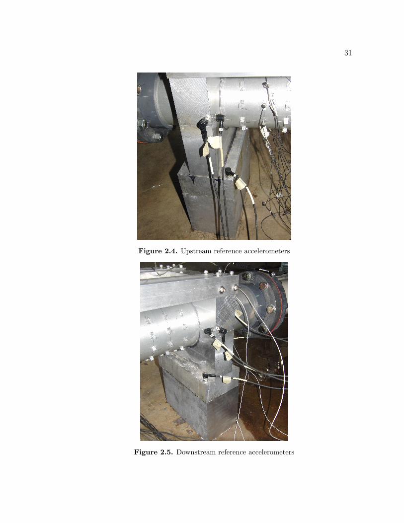
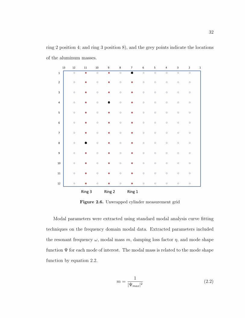
2.1 Pipe flow configuration . . . . . . . . . . . . . . . . . . . . . . . . . 262.2 Test section and wall detail . . . . . . . . . . . . . . . . . . . . . . 272.3 Test section . . . . . . . . . . . . . . . . . . . . . . . . . . . . . . . 302.4 Upstream reference accelerometers . . . . . . . . . . . . . . . . . . . 312.5 Downstream reference accelerometers . . . . . . . . . . . . . . . . . 312.6 Unwrapped cylinder measurement grid . . . . . . . . . . . . . . . . 322.7 (2,1) mode shape and sensitivity function . . . . . . . . . . . . . . . 372.8 Measured and processed hydrophone data . . . . . . . . . . . . . . 41

3.1 Surface roughness profiles . . . . . . . . . . . . . . . . . . . . . . . 453.2 Smooth aluminum plate surface profile . . . . . . . . . . . . . . . . 453.3 Nonskid tape surface profile . . . . . . . . . . . . . . . . . . . . . . 463.4 Smooth Aluminum plate surface profile . . . . . . . . . . . . . . . . 463.5 Smooth Aluminum plate spatial transform . . . . . . . . . . . . . . 473.6 Smooth pipe flow spectrogram . . . . . . . . . . . . . . . . . . . . . 493.7 Fully rough pipe flow spectrogram . . . . . . . . . . . . . . . . . . . 503.8 Smooth pipe flow modal decomposition: ring 1 . . . . . . . . . . . . 503.9 Smooth pipe flow modal decomposition: ring 2 . . . . . . . . . . . . 513.10 Smooth pipe flow modal decomposition: ring 3 . . . . . . . . . . . . 513.11 Fully rough pipe flow modal decomposition: ring 1 . . . . . . . . . . 52

vi

3.12 Fully rough pipe flow modal decomposition: ring 2 . . . . . . . . . . 523.13 Fully rough pipe flow modal decomposition: ring 3 . . . . . . . . . . 533.14 Smooth pipe point pressure spectrum and Chase model . . . . . . . 533.15 Smooth pipe point pressure spectrum and background noise . . . . 543.16 Fully rough pipe point pressure spectrum and background noise . . 543.17 Smooth and fully rough pipe point pressure spectra . . . . . . . . . 553.18 Smooth pipe ambient vibration during flow . . . . . . . . . . . . . . 553.19 Fully rough pipe ambient vibration during flow . . . . . . . . . . . . 563.20 Smooth pipe modal analysis . . . . . . . . . . . . . . . . . . . . . . 583.21 Fully rough pipe modal analysis . . . . . . . . . . . . . . . . . . . . 583.22 Smooth pipe parametric fit to modal data . . . . . . . . . . . . . . 603.23 Fully rough pipe parametric fit to modal data . . . . . . . . . . . . 603.24 (2,1) mode shape and sensitivity function . . . . . . . . . . . . . . . 613.25 (3,3) mode shape and sensitivity function . . . . . . . . . . . . . . . 613.26 Smooth and fully rough low-wavenumber pressure levels . . . . . . . 623.27 180-grit sandpaper 2D surface profile . . . . . . . . . . . . . . . . . 653.28 180-grit sandpaper 3D surface profile . . . . . . . . . . . . . . . . . 653.29 180-grit sandpaper spatial transform . . . . . . . . . . . . . . . . . 663.30 Transitionally rough pipe flow spectrogram . . . . . . . . . . . . . . 663.31 Transitionally rough pipe flow modal decomposition: ring 1 . . . . . 673.32 Transitionally rough pipe flow modal decomposition: ring 2 . . . . . 673.33 Transitionally rough pipe flow modal decomposition: ring 3 . . . . . 683.34 Transitionally rough pipe point pressure spectrum and background

noise . . . . . . . . . . . . . . . . . . . . . . . . . . . . . . . . . . . 683.35 Transitionally rough pipe modal analysis . . . . . . . . . . . . . . . 69

vii

List of Tables

2.1 Test section parameters . . . . . . . . . . . . . . . . . . . . . . . . . 28

3.1 Flow speed average, extrema, and variation . . . . . . . . . . . . . . 433.2 Modal parameters: smooth pipe . . . . . . . . . . . . . . . . . . . . 593.3 Modal parameters: fully rough pipe . . . . . . . . . . . . . . . . . . 593.4 Smooth pipe low-wavenumber normalized pressure levels . . . . . . 633.5 Fully rough pipe low-wavenumber normalized pressure levels . . . . 63

viii

List of Symbols

δ Boundary layer thickness

δ∗ Boundary layer displacement thickness

η Damping loss factor

ν Kinemtic viscosity

ρ Density

τw Wall shear stress

Φ Point pressure spectrum

Ψ Spatial mode shape function

ω Angular frequency

a Pipe radius

c Sound speed

D Pipe diameter

E Young’s modulus

F Modal force

f Friction factor

G Single-sided power spectral density

ix

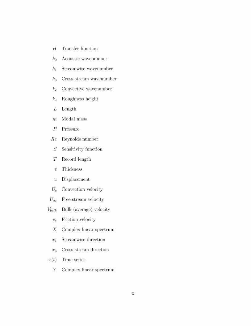
H Transfer function

k0 Acoustic wavenumber

k1 Streamwise wavenumber

k3 Cross-stream wavenumber

kc Convective wavenumber

ks Roughness height

L Length

m Modal mass

P Pressure

Re Reynolds number

S Sensitivity function

T Record length

t Thickness

u Displacement

Uc Convection velocity

U∞ Free-stream velocity

Vbulk Bulk (average) velocity

v∗ Friction velocity

X Complex linear spectrum

x1 Streamwise direction

x3 Cross-stream direction

x(t) Time series

Y Complex linear spectrum

x

Acknowledgments

First, I am grateful to the Applied Research Laboratory and the Walker GraduateAssistantship for supporting the two years of my graduate study. I would like toacknowledge the ARL and Garfield Thomas Water Tunnel management of Dr. EdLiska, Dr. Dick Stern, and Rear Admiral Chuck Brickell, USN (ret.) for theirencouragement of basic research programs at the university labs.

I would like to thank my advisor and the chair of my thesis committee, Dr.Dean Capone, for providing his expertise and direction. Dean’s level-headed anddown to earth advising style have helped me grow as a student and as a researcher,and contributing to his line of work has been a fantastic educational and profes-sional experience for me. I would also like to thank Dr. William Bonness forhis insight and help with everything from experimental setup to data processing.Bill’s intimate knowledge of the experiment and its challenges was invaluable. Dr.Tim Brungart suggested several important corrections and clarifications to thisdocument which improved its clarity and completeness. Dean, Tim, and Bill wereessential in providing corrections and suggestions for improvement throughout theresearch and writing process.

Much credit is due to the enthusiastic professors who have educated me dur-ing my tenure at Penn State, including the chair of the Graduate Program inAcoustics, Dr. Victor Sparrow, who provided guidance and was an integral partof my education. I would also like to acknowledge Drs. Anthony Atchley, KennethBrentner, Thomas Gabrielson, Steven Garrett, Stephen Hambric, Philip Morris,and Karl Reichard.

Finally, I would like to recognize the Garfield Thomas Water Tunnel engineers,students, and staff for their continued assistance and insightful conversations, andAlexandria Salton, who was always nearby for consultation and logisitical help.

xi

Chapter 1Background

1.1 Introduction

1.1.1 Motivation

Turbulent boundary layer noise has been studied for approximately 50 years and

encompasses science and engineering elements from the fields of physical acous-

tics and fluid and structural mechanics. Interest lies primarily in mechanical and

aerospace engineering applications such as air- and water-borne vehicles and fluid

machinery systems. Importance lies in predicting the fluctuating pressures pro-

duced in the turbulent boundary layer and how these pressures can radiate noise

directly or couple to surrounding structures. Interest is generally present in the

noise generation of exterior flow over objects and in interior pipe flow. One of the

motivating factors in initiating the study of boundary layer noise was the develop-

ment of SONAR transducers on moving ships (Skudrzyk and Haddle (1958) [1])

where increased noise levels due to turbulent flow can impair transducer function.

2

Modern engineering concerns include noise and vibration of rotomachinery such as

wind turbines, fluid machinery systems such as pipelines, and passenger vehicles

such as aircraft interior cabin noise.

The state of the art thus far has failed to produce a fully deterministic theory

of turbulence, and it is not yet possible to analytically predict the pressure fluc-

tuations in turbulent flow. Scientists and engineers in the field must often rely

on empirical evidence from flow measurements to perform analyses. Experiments

performed for both internal and external flow configurations in air and water have

led to a number of models, for example, those proposed by Corcos (1963) [2], Chase

(1987) [3], and Smol’yakov (2000) [4], which can be used to predict unsteady pres-

sure levels. There is some disagreement between these models, and modifications

continue to be made as new experimental results become available.

Uncertainty persists in the low-wavenumber region and acoustic domain of

boundary layer pressure fluctuations, where levels are much lower than peak con-

vective levels and are thus very difficult to measure. These low-wavenumber pres-

sures are defined relative to the acoustic wavenumber and translate at speeds near

the ambient sound speed of the medium, where the acoustic wavenumber k0 = ω/c,

ω is the angular frequency, and c is the sound speed. Fluctuations translated at

the convection velocity Uc are referred to as convective pressures and contain most

of the energy in the turbulent boundary layer pressure spectrum. Ko (1993) [5]

defines the frequency dependent convection velocity based on measurements by

Bull (1967) [6] as shown in equation 1.1,

Uc = U∞(0.6 + 0.4e−0.8ωδ∗/U∞) (1.1)

3

where δ∗ is the boundary layer displacement thickness and U∞ is the free-stream

velocity.

Wavenumbers defined by speeds on the order of the mean flow speed are known

as hydrodynamic wavenumbers where the convective wavenumber kc = ω/Uc. De-

spite being low in level and inefficient direct radiators of sound, low-wavenumber,

long wavelength turbulent fluctuations are important because they may couple

to surrounding structures and produce additional noise or vibration. This low-

wavenumber coupling effect is exploited as a method of measuring those very pres-

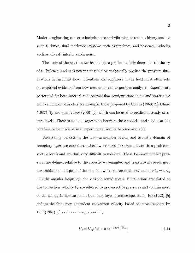
sures. The turbulent boundary layer wavenumber-frequency spectrum is shown

schematically in figure 1.1 versus streamwise wavenumber k1.

k1ω/Ucω/c

P(k,ω)

Acousticdomain

Low-wavenumber(subconvective)

region

Convectiveregion

Hydrodynamicdomain

Viscousregion

Figure 1.1. Turbulent boundary layer wavenumber-frequency spectrum

4

Also of interest and continuing study are the effects of surface roughness on

boundary layer noise. Roughness in flow may be a uniformly distributed field of

small elements (e.g., sandpaper) or more widely spaced discrete bumps or ridges

(e.g., bosses or barnacles; pipe flange discontinuities). While larger discrete ele-

ments such as abrupt geometry changes may affect the acoustics of a hydrody-

namic system, the effects are likely to be characterized by a change in the mean

flow conditions and will vary based on local conditions, requiring an independent

analysis of each configuration. A uniform field of roughness elements will alter the

wavenumber-frequency spectrum of the turbulent boundary layer itself in a manner

that is general and reproducible. The present study is concerned with smooth and

uniformly rough surfaces with roughness scales of interest on the order of one to

ten times the viscous sublayer thickness in order to produce hydraulically smooth

and fully rough surfaces.

Very little modeling of roughness-generated noise has been done, and more

experimental measurements will be needed to produce a widely accepted model for

a range of realistic roughness scales and distributions. A rigorous quantification

of surface roughness that will allow experimental reproducibility may be necessary

in the development of a valid roughness-generated noise model.

It should be noted before proceeding that the present study is concerned with

fully developed turbulent pipe flow, which is not strictly speaking the same as

turbulent boundary layer flow. A turbulent boundary layer over a flat plate will

grow unbounded as flow propagates downstream; the boundary layer in turbulent

pipe flow will eventually converge to the center of the pipe after some inlet length,

after which the velocity profile remains constant. The utility of performing pipe

5

flow measurements is in the extension of fundamental knowledge of turbulent flow,

which can be applied to other interior and exterior flow configurations.

1.1.2 Goals

The present study has two specific goals: to corroborate measurements made by

Bonness, et al. (2010) [7] of the low-wavenumber fluctuating pressure levels in

a turbulent flow over a smooth surface, and to provide low-wavenumber pressure

data for flow over transitionally rough and fully rough surfaces. Bonness utilized

a thin, simply supported cylindrical shell as part of a piping system to measure

the response to fully developed turbulent pipe flow in water driven by static head.

A similar setup is employed in the present study, with the application of two

types of uniform surface roughness in addition to measurements on the smooth

pipe. The radial vibration of the pipe is measured via rings of accelerometers

and a circumferential modal decomposition is performed on the measured data to

extract the modal response of the structure. The physical parameters of the system

are measured using a standard roving force-hammer modal analysis on the fluid

filled pipe without flow. The fluid-structure coupling action of low-wavenumber,

long wavelength pressures allows those pressures to be measured inversely in this

manner.

These data sets will potentially allow for the updating of current models of the

turbulence pressure spectrum and may aid in the development of future models

which may include surface roughness parameters. Models that accurately predict

low-wavenumber pressure fluctuations allow designers and engineers to estimate a

6

priori what noise levels a fluid machinery system will produce or what acoustic

signature a vehicle may have. This knowledge will enable designers to understand

how hydrodynamic and acoustic pressures may couple to structural resonances,

which at low Mach number is a low-wavenumber phenomenon.

1.2 Literature review

1.2.1 Previous work

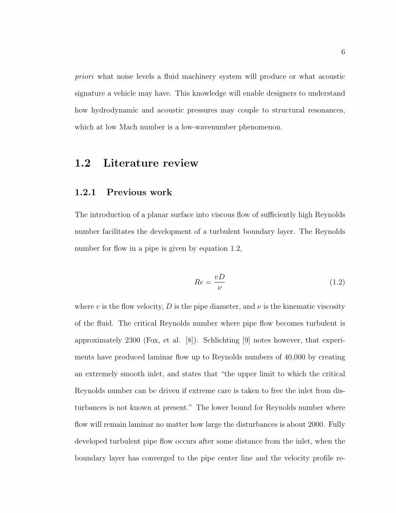
The introduction of a planar surface into viscous flow of sufficiently high Reynolds

number facilitates the development of a turbulent boundary layer. The Reynolds

number for flow in a pipe is given by equation 1.2,

Re =vD

ν(1.2)

where v is the flow velocity, D is the pipe diameter, and ν is the kinematic viscosity

of the fluid. The critical Reynolds number where pipe flow becomes turbulent is

approximately 2300 (Fox, et al. [8]). Schlichting [9] notes however, that experi-

ments have produced laminar flow up to Reynolds numbers of 40,000 by creating

an extremely smooth inlet, and states that “the upper limit to which the critical

Reynolds number can be driven if extreme care is taken to free the inlet from dis-

turbances is not known at present.” The lower bound for Reynolds number where

flow will remain laminar no matter how large the disturbances is about 2000. Fully

developed turbulent pipe flow occurs after some distance from the inlet, when the

boundary layer has converged to the pipe center line and the velocity profile re-

7

mains constant. Schlichting [9] reports a requirement that ranges from 25 - 100

pipe diameters from the inlet to achieve fully developed turbulent pipe flow, based

on measurements by Kirsten (1927) [10] and Nikuradse (1932) [11].

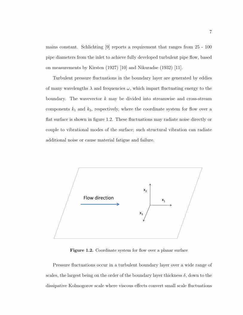
Turbulent pressure fluctuations in the boundary layer are generated by eddies

of many wavelengths λ and frequencies ω, which impart fluctuating energy to the

boundary. The wavevector k may be divided into streamwise and cross-stream

components k1 and k3, respectively, where the coordinate system for flow over a

flat surface is shown in figure 1.2. These fluctuations may radiate noise directly or

couple to vibrational modes of the surface; such structural vibration can radiate

additional noise or cause material fatigue and failure.

Flow direction x1

x3

x2

Figure 1.2. Coordinate system for flow over a planar surface

Pressure fluctuations occur in a turbulent boundary layer over a wide range of

scales, the largest being on the order of the boundary layer thickness δ, down to the

dissipative Kolmogorov scale where viscous effects convert small scale fluctuations

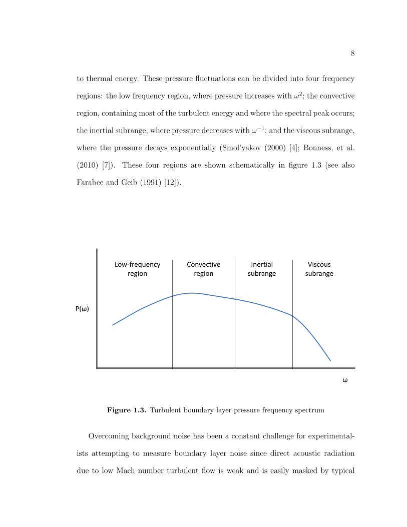
8

to thermal energy. These pressure fluctuations can be divided into four frequency

regions: the low frequency region, where pressure increases with ω2; the convective

region, containing most of the turbulent energy and where the spectral peak occurs;

the inertial subrange, where pressure decreases with ω−1; and the viscous subrange,

where the pressure decays exponentially (Smol’yakov (2000) [4]; Bonness, et al.

(2010) [7]). These four regions are shown schematically in figure 1.3 (see also

Farabee and Geib (1991) [12]).

ω

P(ω)

Low-frequencyregion

Convectiveregion

Viscoussubrange

Inertialsubrange

Figure 1.3. Turbulent boundary layer pressure frequency spectrum

Overcoming background noise has been a constant challenge for experimental-

ists attempting to measure boundary layer noise since direct acoustic radiation

due to low Mach number turbulent flow is weak and is easily masked by typical

9

background noise levels. This problem is evident in both wind and water tunnel

measurements, where facilities may not have been designed for optimal acoustic

performance and where fans and impellers used to circulate the working fluid may

generate substantial noise. Blake (1970) [13] reports that, although using a low-

noise wind tunnel,

The low frequencies were dominated by an unidentified tunnel distur-

bance which was of considerable influence to about 70Hz, also below

70Hz the microphone response began to decrease so that all spectral

data below 70Hz were discarded.

Blake was among the first experimentalists to utilize pinhole transducers to ex-

tend the high frequency measurement range, and was able to report that the space-

time decay rate of small-scale eddies was higher than previously reported. Will-

marth and Woolridge (1962) [14] performed pressure measurements over smooth

and rough surfaces, noting that

...the pressure-fluctuation measurements on the rough steel disk demon-

strate that surface roughness on even a small portion of the wall can

have a profound effect on the fluctuating wall-pressure in the immediate

vicinity.

Like Blake, Willmarth and Woolridge had to discard low frequency data, noting

that the hourly change in sun shining on the wind tunnel test section could alter

fluctuating pressure amplitudes by a factor of 10. This effect is “attributed to

density stratification of the air near the wind-tunnel wall.”

10

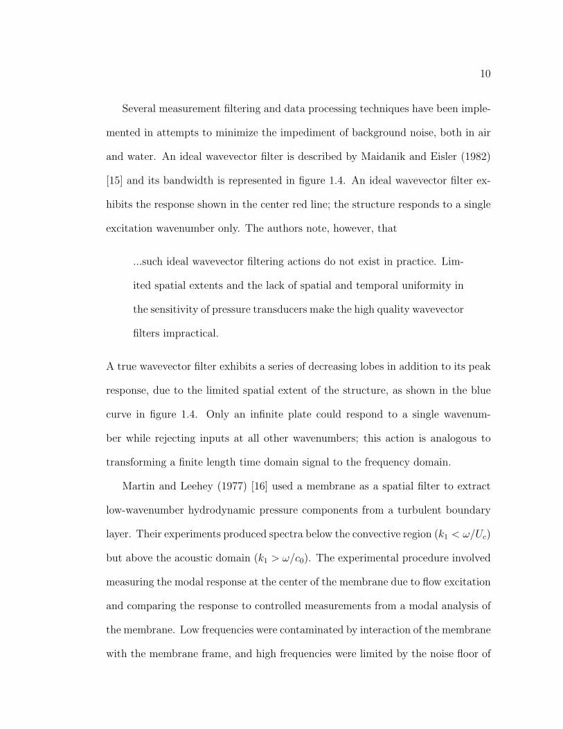
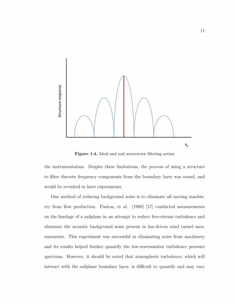
Several measurement filtering and data processing techniques have been imple-

mented in attempts to minimize the impediment of background noise, both in air

and water. An ideal wavevector filter is described by Maidanik and Eisler (1982)

[15] and its bandwidth is represented in figure 1.4. An ideal wavevector filter ex-

hibits the response shown in the center red line; the structure responds to a single

excitation wavenumber only. The authors note, however, that

...such ideal wavevector filtering actions do not exist in practice. Lim-

ited spatial extents and the lack of spatial and temporal uniformity in

the sensitivity of pressure transducers make the high quality wavevector

filters impractical.

A true wavevector filter exhibits a series of decreasing lobes in addition to its peak

response, due to the limited spatial extent of the structure, as shown in the blue

curve in figure 1.4. Only an infinite plate could respond to a single wavenum-

ber while rejecting inputs at all other wavenumbers; this action is analogous to

transforming a finite length time domain signal to the frequency domain.

Martin and Leehey (1977) [16] used a membrane as a spatial filter to extract

low-wavenumber hydrodynamic pressure components from a turbulent boundary

layer. Their experiments produced spectra below the convective region (k1 < ω/Uc)

but above the acoustic domain (k1 > ω/c0). The experimental procedure involved

measuring the modal response at the center of the membrane due to flow excitation

and comparing the response to controlled measurements from a modal analysis of

the membrane. Low frequencies were contaminated by interaction of the membrane

with the membrane frame, and high frequencies were limited by the noise floor of

11

k1

Stru

ctu

re r

esp

on

se

Figure 1.4. Ideal and real wavevector filtering action

the instrumentation. Despite these limitations, the process of using a structure

to filter discrete frequency components from the boundary layer was sound, and

would be revisited in later experiments.

One method of reducing background noise is to eliminate all moving machin-

ery from flow production. Panton, et al. (1980) [17] conducted measurements

on the fuselage of a sailplane in an attempt to reduce free-stream turbulence and

eliminate the acoustic background noise present in fan-driven wind tunnel mea-

surements. This experiment was successful in eliminating noise from machinery

and its results helped further quantify the low-wavenumber turbulence pressure

spectrum. However, it should be noted that atmospheric turbulence, which will

interact with the sailplane boundary layer, is difficult to quantify and may vary

12

widely based on local conditions; thus the reproducibility of this measurement

method is limited.

Farabee and Geib (1991) [12] reported low-wavenumber measurements over

smooth and rough walls in a wind tunnel experiment utilizing a linear wavevector

filter consisting of six large flush-mounted microphones. Measurements were made

for flow velocities from 9.1 - 48.8 m/s for smooth, transitionally rough, and fully

rough surfaces (see section 2.3 and equations 1.14 - 1.16). Farabee and Geib report

increased subconvective and acoustic pressure levels for rough wall conditions, but

remark that acoustic pressures may have been contaminated by facility noise. They

report that

...the acoustic pressures that are measured in the tunnel for a clean

tunnel condition are due to background facility noise and not acoustic

pressures generated by local boundary layer flow. The best that could

be expected from the smooth wall sonic level measurements is to set

the upper bounds on the magnitude of the boundary layer generated

acoustic levels.

Despite some 30 years of study and the implementation of the methods de-

scribed above, accurate measurements of the low-wavenumber pressure levels in a

turbulent boundary layer have remained elusive.

In a recent study by Bonness, et al. (2010) [7], static head from a large reser-

voir was used to drive water through a thin cylindrical shell, eliminating the need

for noisy pumps that generally contaminate acoustic measurements in pipe flow.

The resulting vibration of the shell due to the fluctuating turbulent pressures was

13

measured and used to inversely determine the pressure levels. Similar to Martin’s

and Leehey’s membrane, the modes of the cylinder provide a response to the fluc-

tuating boundary layer pressures at discrete frequencies. Comparing the resulting

vibration to a modal analysis of the cylinder provided physical parameters that

allowed the investigators to predict what fluctuating pressures would produce the

observed vibration. An additional noise cancellation technique was implemented

to reduce the effects of background noise: signals from reference transducers on

nearby structures were not intended to be excited by flow, so any correlated sig-

nals between these and the measurement transducers could be removed. The test

section and procedure developed by Bonness have been adapted for use in this

study.

Results from Bonness’s work provided pressure measurements at lower

wavenumbers than were previously available, and are summarized in figure 1.5,

along with the data reported by Farabee and Geib (1975) [18] and Martin and

Leehey, and the pressure models of Corcos, Chase, and Smol’yakov. Bonness’s

data suggest a normalized low-wavenumber-white, or flat, spectral level of -41 dB.

An important consideration when measuring fluctuating pressures is the lim-

itation that transducer size imposes on the measurement range. Area averaging

of small scale, high frequency turbulence structures will occur over the face of a

transducer and reduce the observed levels. This attenuation was a limiting factor

in many early experiments which used large diameter microphones, which gener-

ally have higher sensitivies than small microphones. The subject of area averaging

is covered in detail by Corcos (1963) [2], and Ko (1993) [5] provides corrections

in the form of spatial pressure sensitivity functions that may be applied to vari-

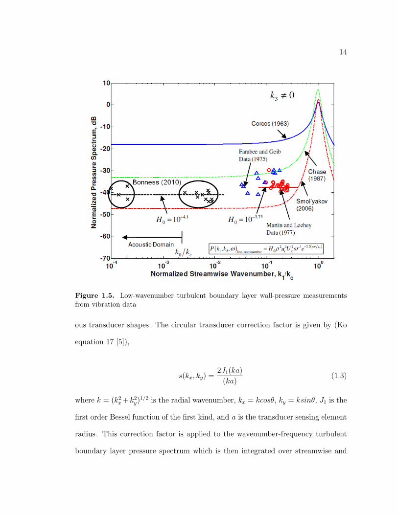
14

Figure 1.5. Low-wavenumber turbulent boundary layer wall-pressure measurementsfrom vibration data

ous transducer shapes. The circular transducer correction factor is given by (Ko

equation 17 [5]),

s(kx, ky) =2J1(ka)

(ka)(1.3)

where k = (k2x +k2

y)1/2 is the radial wavenumber, kx = kcosθ, ky = ksinθ, J1 is the

first order Bessel function of the first kind, and a is the transducer sensing element

radius. This correction factor is applied to the wavenumber-frequency turbulent

boundary layer pressure spectrum which is then integrated over streamwise and

15

cross-stream wavenumbers (k1 and k3) to produce the attenuated point pressure

spectrum which may then be compared with measured spectra. This integration

is given by equation 1.4 (Ko equation 1 [5]),

P (ω) = 2π

∫ ∫S(kx, ky)P (kx, ky, ω)dkxdky (1.4)

where S(kx, ky) = [s(kx, ky)]2 and P is the wavenumber-frequency pressure spec-

trum.

1.2.2 Turbulent boundary layer pressure models

One of the most popular models of the fluctuating pressure in a turbulent bound-

ary layer over a smooth plane surface was proposed by Chase (1980) [19] and was

extended to lower wavenumbers by Chase in 1987 [3] by including compressibility

(acoustic) effects. This model of the pressure spectrum is limited to subconvective

wavenumbers and is not valid at high frequencies, where viscosity becomes impor-

tant. The Chase model consists of two components, one represented by CT which

reflects interactions between turbulent eddies (known as turbulence-turbulence in-

teractions), and one represented by CM which reflects turbulence-mean shear in-

teractions. Howe (1979) [20] proposed a correction to the model, suggesting a low

frequency dependence of ω2 based on an analysis of the fluctuating surface shear

stress, which is dipole in nature. Lysak (2006) [21] added an exponential decay

factor to this modified model to reflect the high frequency, small scale sources in

the viscous subrange. The 1987 Chase model of the wall-pressure wavenumber-

frequency spectrum is given by equation 1.5 (Chase equation 40),

16

P (k, ω) =ρ2v3∗

[k2+ + (bδ)−2]5/2

{[c2

(|kc|k

)2

+ c3

(k

|kc|

)2

+ 1− c2 − c3

](1.5)

CTk2

[k2

+ + (bδ)−2

k2 + (bδ)−2

]+ CM

(k

|kc|

)2

k21

}

where ρ is the fluid density; v∗ is the friction velocity; δ is the boundary layer

thickness; h = 3.0, CTh = 0.014, CMh = 0.466, b = 0.75, and c2 = c3 = 1/6 are

empirical constants based on experimental data; and wavenumbers k =√k2

1 + k23,

k+ = (ω − uk1)2/(hv∗)2 + k2, and

|Kc|2 =

k2 − ω2/c2, k > ω/c

ω2/c2 − k2, k < ω/c

.

The 1987 Chase model, extrapolated to the acoustic domain by Howe (1991) [22]

is given by equation 1.6 (Howe equation 11),

P (k, ω) =ρ2v3∗δ

3

[(k+δ)2 + 1/b2]5/2

[CM(k1δ)

2k2

|k2 − k20|+ ε2k2

0

+ CT (kδ)2 (k+δ)2 + 1/b2

(kδ)2 + 1/b2(1.6)(

c1 +c2|k2 − k2

0|k2

+c3k

2

|k2 − k20|+ ε2k2

0

)]

where c1 = 2/3.

Integration of the wavenumber frequency spectrum over streamwise and cross-

stream wavenumbers produces a function of frequency only, known as the point

pressure frequency spectrum, given by equation 1.7. The point pressure spectrum

is what would be measured by a point pressure transducer; that is, it neglects

any high frequency attenuation that would be introduced by area averaging over a

17

transducer of finite area. The Chase point pressure spectrum is given by equation

1.8 and the Howe modification is given by equation 1.9. The modified Chase-Howe

model with the Lysak correction factor [21] is given by equation 1.10,

Φ(ω) =

∫P (k, ω)dk1dk3 (1.7)

Φ(ω)

ρ2U3∞δ

=

(v∗U∞

)4(( ωδU∞

)2 + α2c

)(( ωδU∞

)2

+ 1)1.5 , αc = 0.2 (1.8)

Φ(ω)

ρ2U3∞δ∗ =

(v∗U∞

)4(ωδ∗

U∞

)2((ωδ

∗

U∞)2 + α2

p

)1.5 , αp = 0.12 (1.9)

Φ(ω)

ρ2U3∞δ∗ =

(v∗U∞

)4(ωδ∗

U∞

)2((ωδ

∗

U∞)2 + α2

p

)1.5 e−2.2(ων/v∗) (1.10)

where ν is the kinematic viscosity of the fluid.

In 2000, Smol’yakov [4] proposed a piecewise model of the pressure spectrum

with separate scaling parameters for each of the three characteristic frequency

dependent ranges, given by equations 1.11 - 1.13 (Smol’yakov equation 18),

Φ(ω)

ρ2v2∗ν

= 1.49× 10−5R2.74θ ω2(1− 0.117R0.44

θ ω1/2), ω < ω0 (1.11)

Φ(ω)

ρ2v2∗ν

= 2.75ω−1.11(1− 0.82e−0.51(ω/ω0−1)), ω0 < ω < 0.2 (1.12)

18

Φ(ω)

ρ2v2∗ν

= (38.9e−8.35ω + 19.6e−3.58ω + 0.31e−2.14ω)(1− 0.82e−0.51(ω/ω0−1)), ω > 0.2

(1.13)

where ω = ων/v2∗, ω0 = 49.35R−0.88

θ , and the Reynolds number Rθ = U0θ/ν where

the momentum thickness θ = 7/9δ∗.

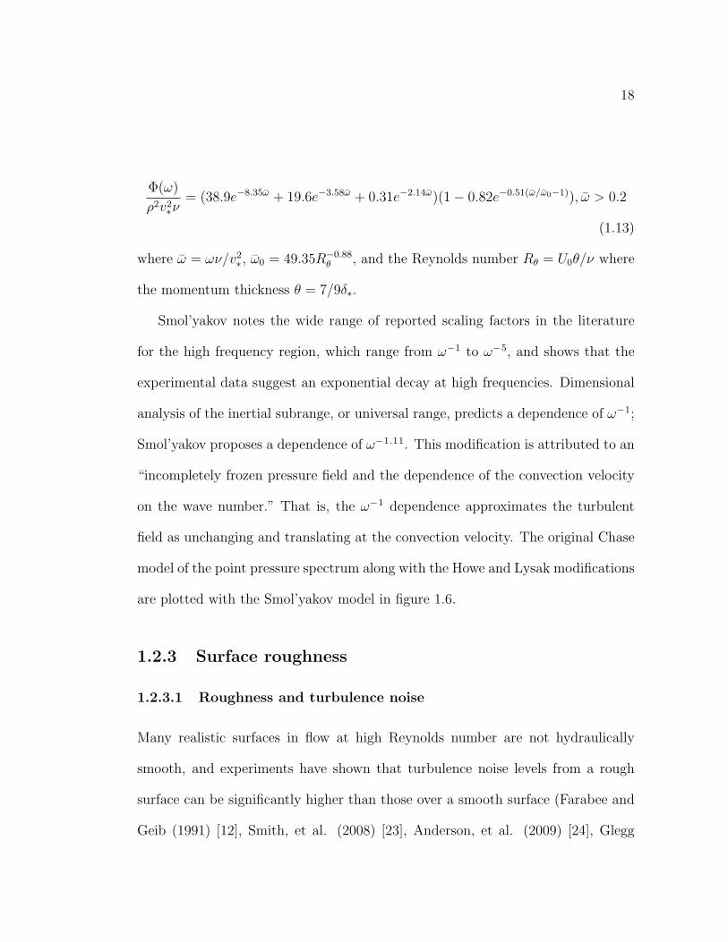
Smol’yakov notes the wide range of reported scaling factors in the literature

for the high frequency region, which range from ω−1 to ω−5, and shows that the

experimental data suggest an exponential decay at high frequencies. Dimensional

analysis of the inertial subrange, or universal range, predicts a dependence of ω−1;

Smol’yakov proposes a dependence of ω−1.11. This modification is attributed to an

“incompletely frozen pressure field and the dependence of the convection velocity

on the wave number.” That is, the ω−1 dependence approximates the turbulent

field as unchanging and translating at the convection velocity. The original Chase

model of the point pressure spectrum along with the Howe and Lysak modifications

are plotted with the Smol’yakov model in figure 1.6.

1.2.3 Surface roughness

1.2.3.1 Roughness and turbulence noise

Many realistic surfaces in flow at high Reynolds number are not hydraulically

smooth, and experiments have shown that turbulence noise levels from a rough

surface can be significantly higher than those over a smooth surface (Farabee and

Geib (1991) [12], Smith, et al. (2008) [23], Anderson, et al. (2009) [24], Glegg

19

Figure 1.6. Turbulent boundary layer pressure models

and Devenport (2009) [25]). Surface roughness increases the resistance to flow

compared to a smooth surface, and the laws of friction depend on the shape and

distribution of roughness elements. Roughness effects are a turbulent flow phe-

nomenon; for laminar flow in a pipe, resistance and the critical Reynolds number

are both independent of roughness.

In terms of scale, a surface can be considered hydrodynamically smooth if

roughness elements are completely contained within the viscous sublayer. In this

range, within the viscous sublayer, the wall shear stress is dominated by laminar

friction. A second region exists some distance further from the wall, where shear

stresses are dominated by turbulent friction. A surface with roughness elements

20

Viscous sublayer

Inertial sublayer

r

U∞

Figure 1.7. Turbulent boundary layer velocity profile

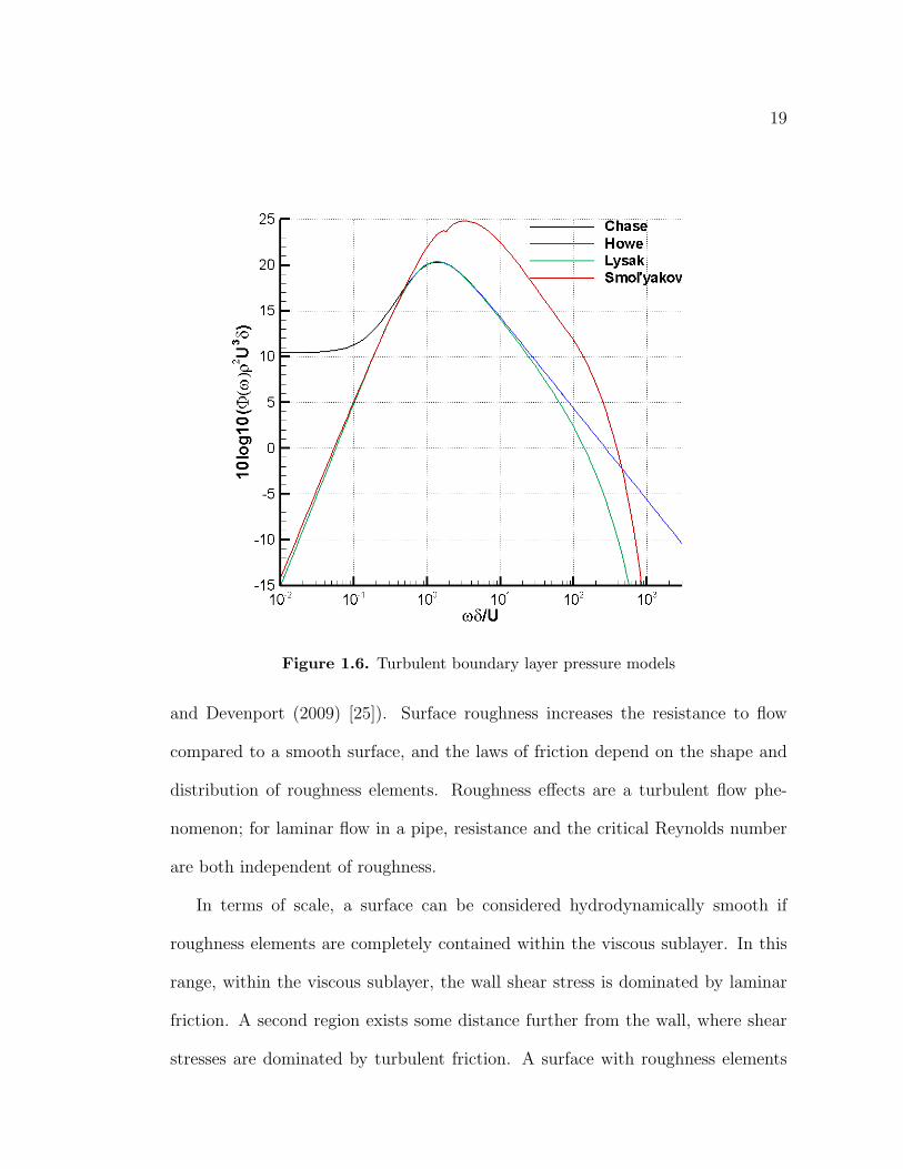
extending into this range is considered to be fully rough, and a transition region

exists between these two limits. The velocity profile of a turbulent boundary layer

is shown in figure 1.7, where the viscous sublayer and inertial sublayer thicknesses

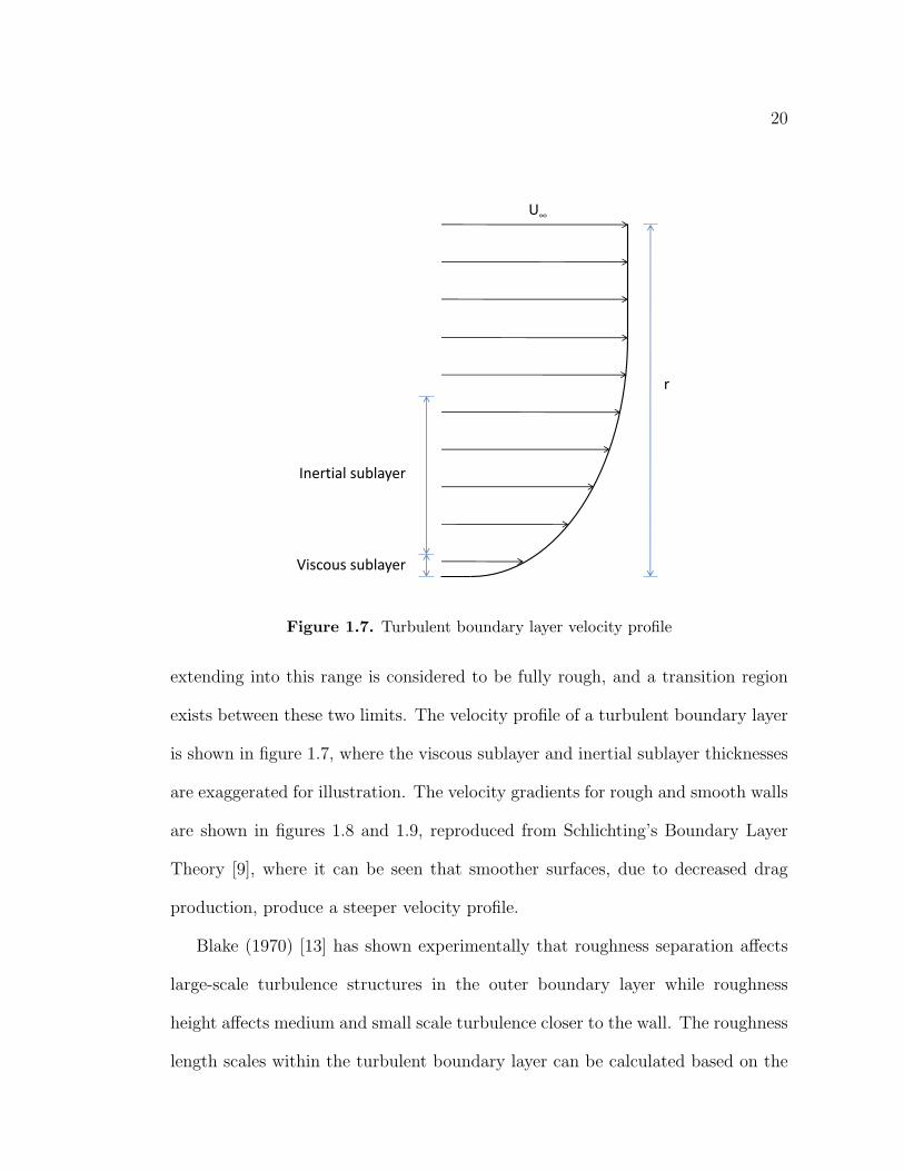
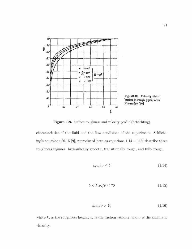
are exaggerated for illustration. The velocity gradients for rough and smooth walls

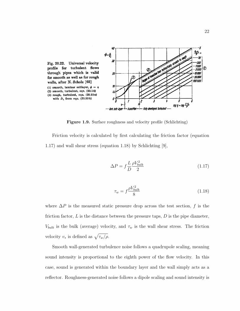
are shown in figures 1.8 and 1.9, reproduced from Schlichting’s Boundary Layer

Theory [9], where it can be seen that smoother surfaces, due to decreased drag

production, produce a steeper velocity profile.

Blake (1970) [13] has shown experimentally that roughness separation affects

large-scale turbulence structures in the outer boundary layer while roughness

height affects medium and small scale turbulence closer to the wall. The roughness

length scales within the turbulent boundary layer can be calculated based on the

21

Figure 1.8. Surface roughness and velocity profile (Schlichting)

characteristics of the fluid and the flow conditions of the experiment. Schlicht-

ing’s equations 20.15 [9], reproduced here as equations 1.14 - 1.16, describe three

roughness regimes: hydraulically smooth, transitionally rough, and fully rough,

ksv∗/ν ≤ 5 (1.14)

5 < ksv∗/ν ≤ 70 (1.15)

ksv∗/ν > 70 (1.16)

where ks is the roughness height, v∗ is the friction velocity, and ν is the kinematic

viscosity.

22

Figure 1.9. Surface roughness and velocity profile (Schlichting)

Friction velocity is calculated by first calculating the friction factor (equation

1.17) and wall shear stress (equation 1.18) by Schlichting [9],

∆P = fL

D

ρV 2bulk

2(1.17)

τw = fρV 2

bulk

8(1.18)

where ∆P is the measured static pressure drop across the test section, f is the

friction factor, L is the distance between the pressure taps, D is the pipe diameter,

Vbulk is the bulk (average) velocity, and τw is the wall shear stress. The friction

velocity v∗ is defined as√τw/ρ.

Smooth wall-generated turbulence noise follows a quadrupole scaling, meaning

sound intensity is proportional to the eighth power of the flow velocity. In this

case, sound is generated within the boundary layer and the wall simply acts as a

reflector. Roughness-generated noise follows a dipole scaling and sound intensity is

23

proportional to the sixth power of the flow velocity. Roughness-generated sound is

generated at the surface boundary and is primarily due to scattering of convective

pressures which distributes energy to lower wavenumbers (Howe (1991) [22], Smith,

et al. (2008) [23], Anderson, et al. (2009) [24]). Anderson, et al. add that each

roughness element may be viewed as an individual dipole source where the resultant

sound is a summation of the noise generated over each element. However, direct

noise radiation from low Mach number turbulent flow is very weak, and an increase

in surface roughness will not greatly enhance this noise. It is likely the scattering

of convective pressures to lower wavenumbers by surface roughness which may

increase fluid-structure interaction that is particularly important.

Roughness effects may be more significant in water flow than in air for a given

element size, where boundary layers are generally thinner due to increased fluid

density which increases relative roughness heights. The present study seeks to

quantify smooth, transitionally rough, and fully rough surfaces, and how varying

surface roughness affects the pressure spectrum in a turbulent boundary layer,

particularly at low wavenumbers.

1.2.3.2 Response to a step change in roughness

The 1.2 m test section interior was roughened and the adjacent piping segments

were left untreated, introducing a step change in surface roughness. The response

of a turbulent boundary layer to a step change in roughness has been described by

Antonia and Luxton (1971) [26] [27] and Cheng and Castro (2002) [28]. Measure-

ments suggest an inner layer which forms on the leading edge of the roughness step

and propagates downstream into the mean flow. Thus, effects on the mean flow

24

take some time to reach a steady state, while small scale turbulence production

and scattering of convective structures happens immediately. This scattering is

the primary source of increased low-wavenumber pressures.

Chapter 2Experimental methods and

mathematical formulations

2.1 Pipe configuration

A cylindrical aluminum test section is used to inversely measure low-wavenumber

fluctuating turbulent wall-pressures in pipe flow. The thin aluminum shell is placed

in series within a longer piping system and its response to flow is measured by a

series of circumferentially positioned accelerometers. At low Mach number, low-

wavenumber pressures do not radiate strongly compared to convective pressures,

but do couple well to structures in flow when the structural length scale is compara-

ble to the wavelength of the fluctuating pressures. Therefore, in the present setup,

the cylinder acts as a structural wavevector filter to measure the low-wavenumber

pressure spectrum at a series of discrete frequencies corresponding to the resonant

modes of the shell.

Performing the experiment in water rather than air allows the low-wavenumber

26

region of the pressure spectrum to be more easily measured for two reasons. The

convective region is shifted up due to the decrease in practical flow speeds compared

to air flow, and the acoustic domain is shifted down due to the higher sound speed

in water (1480 m/s) than air (340 m/s). Both of these effects extend the effective

range of the low-wavenumber region.

1.2m aluminum pipe14m = 93 pipe diameters To reserve tank

48” Water Tunnel = 400 kL reservoir

Upstream flow conditioning plate 61 cm test section

Figure 2.1. Pipe flow configuration

Integral to the present experiment is the utilization of static head to drive water

flow through the measurement apparatus, eliminating the need for noisy machinery

to move the fluid. As shown in figure 2.1, a 400,000 L reservoir drives water through

the 61 cm long, 150 mm diameter test section producing fully developed turbulent

pipe flow with an average free stream velocity of approximately 6 m/s. The present

configuration provides approximately 93 pipe diameters from the upstream flow

27

conditioning plate to the start of the test section. A perforated 1-7-13 Laws type

flow conditioning plate (Laws (1990) [29]) is installed after the upstream gate

valve to minimize the effect of the valve and preceding 90◦ bend on the mean flow.

Care is taken to fare the transition at the flange between the test section and the

upstream pipe section to minimize any potential discontinuity.

a

t

L

ttg

tS40

3 2 1

Figure 2.2. Test section and wall detail

The 61 cm long cylindrical aluminum test section is machined into the center

of a 1.2 m long, 150 mm diameter schedule 40 aluminum pipe to a thickness of

3.2 mm with grooves machined at each end to a thickness of 0.64 mm to simulate

simply supported boundary conditions (see figures 2.2 and 2.3 and table 2.1). The

28

Table 2.1. Test section parameters

Parameter Symbol ValueLength L 61 cmRadius a 76 mm

Schedule 40 pipe thickness tS40 7.2 mmWall thickness t 3.2 mm

Groove thickness tg 0.64 mmYoung’s modulus E 69 GPa

Poisson’s ratio ν 0.3Aluminum density ρ 2700 kg/m3

test section is outfitted with three circumferential rings of 12 accelerometers (PCB

Piezotronics model 352C67; see figures 2.2 and 2.6). The test section arrangement

is intended to minimize translation and extraneous vibration of the test section.

The supporting structure is outfitted with six PCB 607A11 accelerometers for

noise removal purposes (reference accelerometers), one oriented in each direction

on the upstream and downstream supports (see figures 2.4 and 2.5). Pressures

from the turbulent boundary layer are the only intended vibration input to the

cylindrical test section, so any coherent signals between the circumferential mea-

surement accelerometers and the reference accelerometers can be removed. Two

flush mounted hydrophones (PCB 105M147) record the boundary layer pressures

directly and provide the point pressure spectrum in the middle and high frequency

ranges. Each hydrophone has an adjacent reference accelerometer to facilitate the

removal of vibration induced noise from the point pressure spectrum.

To mitigate the effects of any possible uneven mass-loading from the accelerom-

eters, each location on the aluminum test section not occupied by an accelerometer

is outfitted with a small aluminum mass. This allows the 156-point measurement

29

grid over the whole cylinder to be evenly loaded, where a flat spot has been ma-

chined at each grid point to aid in the placement of accelerometers and masses.

Flow speeds are measured via a pitot-static probe at the centerline of the pipe,

just downstream of the test section. A pitot-static tube measures total (stagnation)

and static pressure through openings on the front and side of the tube, respectively.

The stagnation pressure is related to the static and dynamic pressures by equation

2.1,

Ptotal = Pstatic +1

2ρv2 (2.1)

where the second term on the right is the dynamic pressure and can be solved for

velocity.

All flow measurements are recorded simultaneously in the time domain onto

a National Instruments PXI 1033 data acquisition system and are processed in

Matlab.

2.2 Modal analysis

A thin aluminum cylinder is utilized in this experiment as a spatial filter. In order

to extract the fluctuating turbulent boundary layer pressures from flow-induced

vibration levels, its modal parameters must first be measured. The parameters

of interest include the resonant frequency, modal mass, damping loss factor, and

mode shape function for each mode. Radiation loss factors are assumed to be

negligible for the modes of interest. A roving force hammer modal analysis was

performed on the fluid-filled pipe under each of the three roughness conditions; a

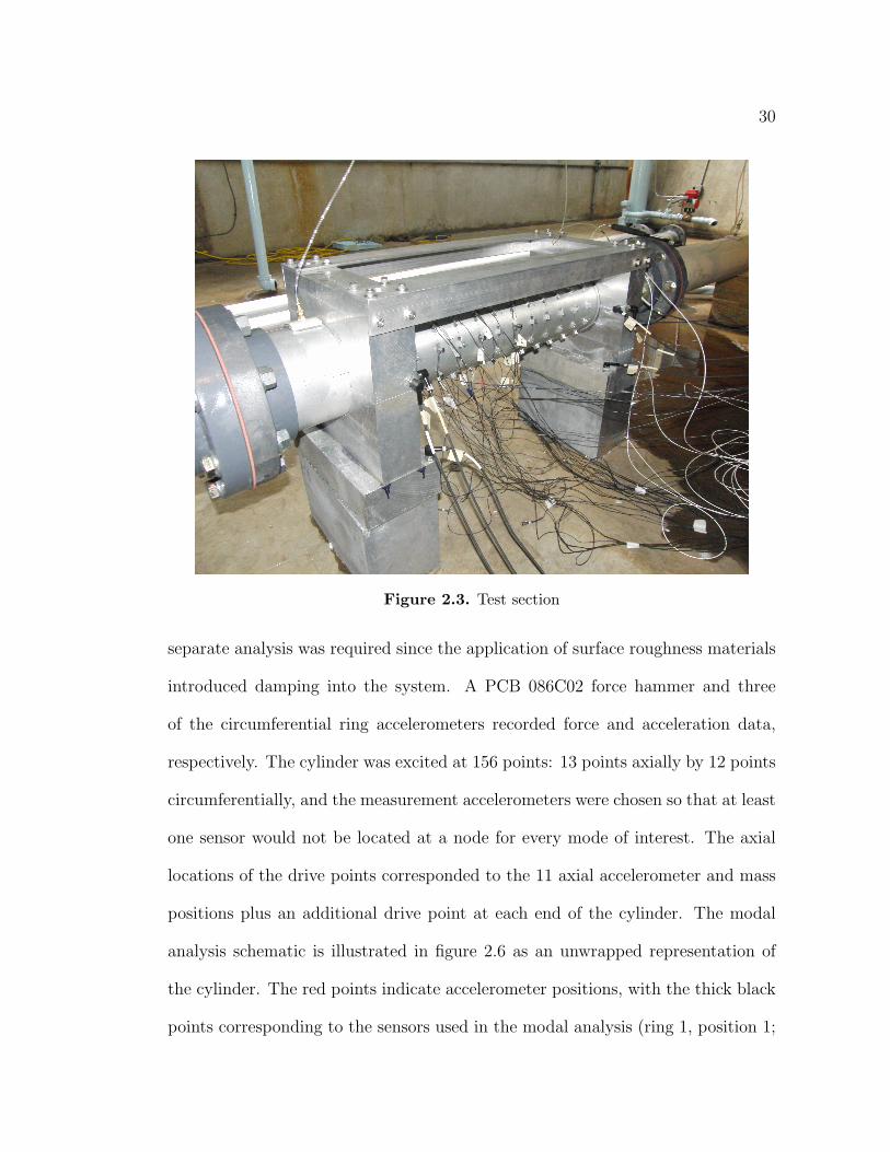
30

Figure 2.3. Test section

separate analysis was required since the application of surface roughness materials

introduced damping into the system. A PCB 086C02 force hammer and three

of the circumferential ring accelerometers recorded force and acceleration data,

respectively. The cylinder was excited at 156 points: 13 points axially by 12 points

circumferentially, and the measurement accelerometers were chosen so that at least

one sensor would not be located at a node for every mode of interest. The axial

locations of the drive points corresponded to the 11 axial accelerometer and mass

positions plus an additional drive point at each end of the cylinder. The modal

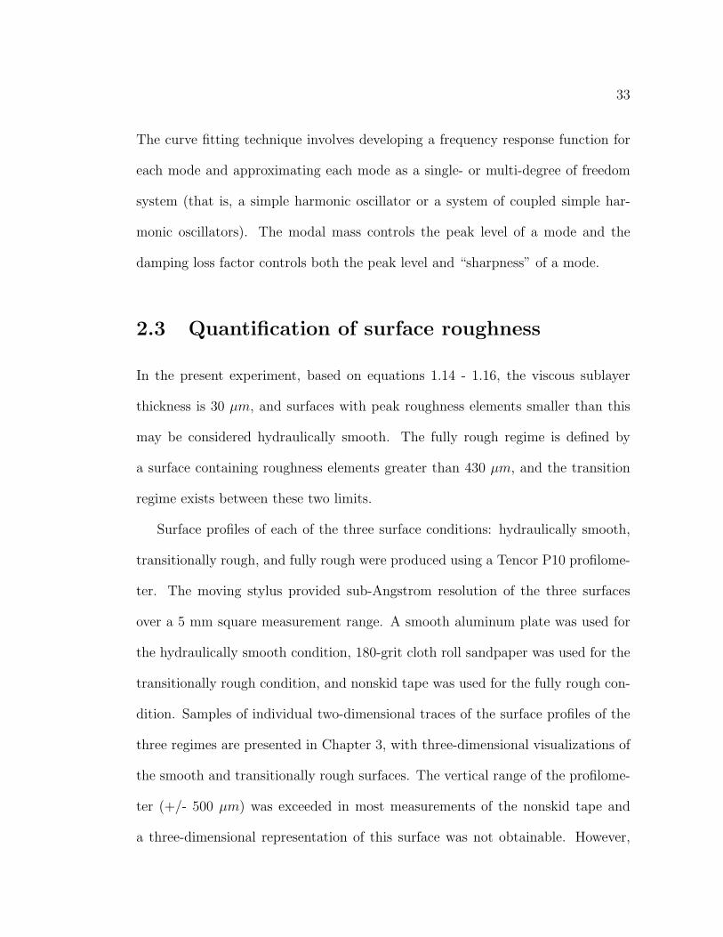
analysis schematic is illustrated in figure 2.6 as an unwrapped representation of

the cylinder. The red points indicate accelerometer positions, with the thick black

points corresponding to the sensors used in the modal analysis (ring 1, position 1;

31

Figure 2.4. Upstream reference accelerometers

Figure 2.5. Downstream reference accelerometers

32

ring 2 position 4; and ring 3 position 8), and the grey points indicate the locations

of the aluminum masses.

13 12 11 10 9 8 7 6 5 4 3 2 1

2

3

4

5

6

7

8

9

10

11

12

Ring 1Ring 2Ring 3

1

Figure 2.6. Unwrapped cylinder measurement grid

Modal parameters were extracted using standard modal analysis curve fitting

techniques on the frequency domain modal data. Extracted parameters included

the resonant frequency ω, modal mass m, damping loss factor η, and mode shape

function Ψ for each mode of interest. The modal mass is related to the mode shape

function by equation 2.2.

m =1

|Ψmax|2(2.2)

33

The curve fitting technique involves developing a frequency response function for

each mode and approximating each mode as a single- or multi-degree of freedom

system (that is, a simple harmonic oscillator or a system of coupled simple har-

monic oscillators). The modal mass controls the peak level of a mode and the

damping loss factor controls both the peak level and “sharpness” of a mode.

2.3 Quantification of surface roughness

In the present experiment, based on equations 1.14 - 1.16, the viscous sublayer

thickness is 30 µm, and surfaces with peak roughness elements smaller than this

may be considered hydraulically smooth. The fully rough regime is defined by

a surface containing roughness elements greater than 430 µm, and the transition

regime exists between these two limits.

Surface profiles of each of the three surface conditions: hydraulically smooth,

transitionally rough, and fully rough were produced using a Tencor P10 profilome-

ter. The moving stylus provided sub-Angstrom resolution of the three surfaces

over a 5 mm square measurement range. A smooth aluminum plate was used for

the hydraulically smooth condition, 180-grit cloth roll sandpaper was used for the

transitionally rough condition, and nonskid tape was used for the fully rough con-

dition. Samples of individual two-dimensional traces of the surface profiles of the

three regimes are presented in Chapter 3, with three-dimensional visualizations of

the smooth and transitionally rough surfaces. The vertical range of the profilome-

ter (+/- 500 µm) was exceeded in most measurements of the nonskid tape and

a three-dimensional representation of this surface was not obtainable. However,

34

based on limited measurements and the limitation of the profilometer, it can be

stated with confidence that the nonskid tape provides a fully rough surface, with

elements consistently greater than 430 µm in height, and often greater than 1 mm

peak-to-peak.

A spatial transform of the three-dimensional surface profile provides a visual-

ization of the distribution of roughness element sizes. A random distribution of

roughness element sizes would transform to a flat surface, similar to the flat fre-

quency response of a random time series. Conversely, a surface sinusoidal in one

dimension would exhibit a ridge in the spatial transform, and a surface sinusoidal

in both dimensions (producing a series of uniform bumps) would have two perpen-

dicular ridges, representing the length scales of the elements in each dimension.

Surface profile figures are presented in Chapter 3.

2.4 Inverse method of determining turbulent

boundary layer fluctuating pressure levels

In addition to measuring the turbulent wall-pressure point spectra directly via

hydrophones, the cylindrical test section’s modal response to the turbulent pipe

flow excitation is recorded via three circumferential rings of 12 accelerometers each.

Based on the modal parameters obtained from the experimental modal analysis,

the turbulent wall-pressure levels required to cause the observed vibration can be

determined. A circumferential modal decomposition is performed on the vibration

data, in which the recorded time series for each ring is transformed to the frequency

35

domain. The use of 12 accelerometers per ring and the positioning of the three

rings allow modes up to order n = 6 and m = 5 to be resolved before aliasing

occurs.

The mass-normalized spatial mode shape functions Ψn(x1, x3), having a max-

imum value of one, can be translated to sensitivity functions Sn(k1, k3) in the

wavenumber domain via a spatial transform, shown in equation 2.3. Hwang and

Maidanek (1990) [30] provide a relation for the turbulent boundary layer fluctuat-

ing pressures, the sensitivity functions, and the modal force, shown in equation 2.4,

where the normalized pressure spectrum P (k1, k3) is defined by equation 2.5. The

modal force Fn is related to the cylinder displacement and modal parameters by

equation 2.6, based on the Frequency Response Function (FRF) given by equation

2.7 (Ewins [31]) and the relation to the force at a point β, Fn(ω) = Ψn(β)F (β, ω),

S(k1, k3) =

∫ ∫A

Ψn(x1, x3)eik1x1eik3x3dx1dx3 (2.3)

|Fn(ω)|2 =

∫ ∫∞P (k1, k3, ω)|Sn(k1, k3)|2dk1dk3 (2.4)

P (k1, k3, ω) = P (k1, k3)Φpp(ω) (2.5)

un(α, ω) =1

mn

Ψn(α)Fn(ω)[− ω2 + ω2

n + iηnωnω] (2.6)

un(α, ω)

F (β, ω)=

1

mn

Ψn(α)Ψn(β)[− ω2 + ω2

n + iηnωnω] (2.7)

36

where un is the displacement, mn, ηn, and ωn are the modal mass, loss factor,

and resonant frequency of each mode, respectively, and α and β are points on the

structure. The FRF relates the displacement at a point α to the force at a point

β as a function of frequency.

Accelerance can be computed from equation 2.7 by relating displacement and

acceleration through a factor of ω2 and compared to the accelerance obtained

from the roving force hammer modal analysis. The modal parameters are then

adjusted until the two sets of response curves match, where the calculated curve

is a sum of the FRFs of all modes. Once the modal parameters are known, the

modal force can be calculated using the measured peak displacements un from flow-

induced vibration using equation 2.6 and compared to the modal force computed

by equation 2.4, where P (k1, k3, ω) is assumed to be wavenumber-white. This

wavenumber-white, or constant amplitude pressure level is given by equation 2.8

[32],

P (k1, k3, ω) = H0ρ2u4

τU2c ω−3e−2.2(ων/uτ ) (2.8)

where H0 is the constant level, 10−4.1, based on an assumed level of -41 dB. Fi-

nally, this input pressure level is adjusted until the forcing function based on the

measured vibration equals the predicted level based on the wavenumber-frequency

pressure spectrum.

The value of the streamwise wavenumber at each mode corresponding to the

peak pressure level is computed from the sensitivity function, which is a function

of both streamwise and cross-stream wavenumbers, k1 and k3. Pressure levels are

37

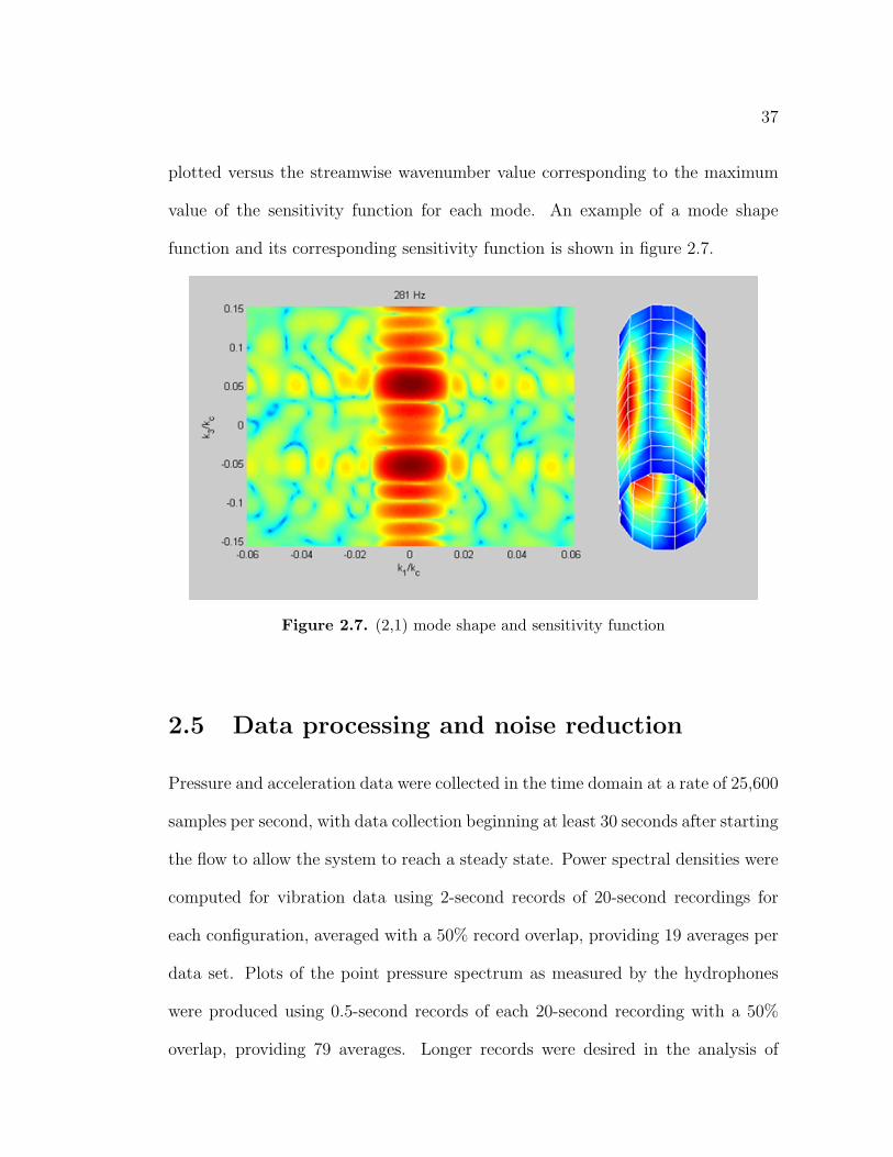
plotted versus the streamwise wavenumber value corresponding to the maximum

value of the sensitivity function for each mode. An example of a mode shape

function and its corresponding sensitivity function is shown in figure 2.7.

Figure 2.7. (2,1) mode shape and sensitivity function

2.5 Data processing and noise reduction

Pressure and acceleration data were collected in the time domain at a rate of 25,600

samples per second, with data collection beginning at least 30 seconds after starting

the flow to allow the system to reach a steady state. Power spectral densities were

computed for vibration data using 2-second records of 20-second recordings for

each configuration, averaged with a 50% record overlap, providing 19 averages per

data set. Plots of the point pressure spectrum as measured by the hydrophones

were produced using 0.5-second records of each 20-second recording with a 50%

overlap, providing 79 averages. Longer records were desired in the analysis of

38

vibration data to provide higher frequency resolution for the determination of

peak vibration amplitudes.

The complex linear spectrum Xm is computed from the time domain signal

x(t) by equation 2.9 (Gabrielson (2010) [33]) and the autospectral density, or

autospectrum, is computed by equation 2.10 where T is the record length. The

cross-spectral density, or cross-spectrum, is computed from two linear spectra by

equation 2.11 where * denotes a complex conjugate, and the transfer function

is defined by equation 2.12 where the overbar denotes an average. The transfer

function has a maximum value of one, and is scaled by using equation 2.13.

Xm(f) =

∫∞x(t)e−i2πftdt (2.9)

Gxx(f) =2

T|Xm(f)|2 (2.10)

Gxy(f) =2

TX(f)∗Y (f) (2.11)

Hxy(f) =Gxx(f)

Gxy(f)(2.12)

Hxy(f) =Gxy(f)

Gxx(f)

√|Gxx(f)| (2.13)

This analysis is performed on each ring of 12 accelerometers, iteratively tak-

ing each accelerometer as the reference signal Gxx. This produces 12 sets of 12

39

transfer functions for each ring of accelerometers which are each decomposed into

their Fourier components by equation 2.14 (Bonness (2009) [32]) and averaged to

produce the modal response of the cylinder,

Hn(f) =1

N

N∑y=1

Hxy(f)e−i2π(n−1)(y−1)/N (2.14)

where y is the accelerometer number, N is the number of accelerometers, and n is

the mode number.

A noise cancellation technique described by Bendat and Piersol [34] was em-

ployed in which coherent signals between measurement and reference transducers

can be removed. This process involves computing the cross-spectral density matrix

between each measurement transducer and reference transducer, iteratively remov-

ing the coherent noise component from each signal. The form of this cross-spectral

density matrix for an arbitrary number of measurement and reference transducers

is shown in equation 2.15,

Gxy(n)!(f) = Gxy(n−1)!(f)−Gxn(n−1)!(f)Gny(n−1)!(f)

Gnn(n−1)!(f)(2.15)

where Gxy represents the cross-spectrum between transducers x and y and Gnn

represents the autospectrum of a noise transducer.

This procedure is followed for each of the 36 accelerometers measuring the flow-

induced vibration of the cylinder, iteratively removing noise measured by the six

reference accelerometers on the supporting structure. The process is repeated for

the two hydrophones, removing noise measured by the corresponding adjacent ref-

erence accelerometer. An additional technique can be applied to the hydrophones:

40

acoustic noise is made up of primarily plane waves and is coherent between the

hydrophones, whereas hydrodynamic boundary layer pressures consist of random

eddies of various wavelengths, and are largely incoherent between the two sensors.

Thus, the above procedure can be applied between the hydrophones themselves.

The two-sensor model is provided by Bendat and Piersol and is shown in equation

2.16,

Gxx(f) = Gxmxm(f)− |Gxmnm(f)|2

Gnmnm(f)(2.16)

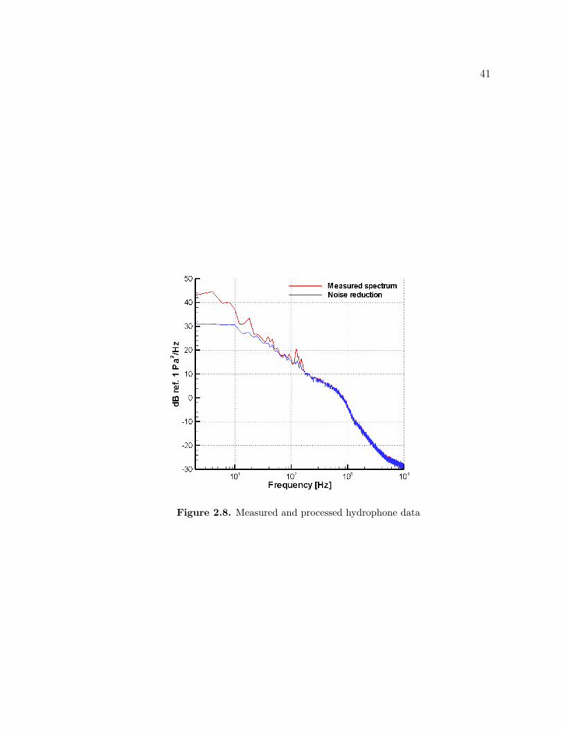
These noise cancellation procedures allow the signal to noise ratio in both the

vibration and pressure data to be improved, primarily in the low frequency region,

and help ensure that the measured vibrations are mainly caused by turbulent pipe

flow pressures. The result of this procedure is shown in figure 2.8 which shows

measured and processed point pressure spectra (for the smooth flow condition).

41

Figure 2.8. Measured and processed hydrophone data

Chapter 3Results

3.1 Measurement results

The present experiment utilizes a number of measurement transducers including

hydrophones which record the turbulent wall-pressure point spectra directly, ac-

celerometers which measure the cylinder’s vibration response due to the turbu-

lent pipe flow pressures and the ambient vibration of the support structure, and

a pitot-static probe for measuring flow speed. A multi-step analysis procedure

is implemented involving the circumferential modal decomposition of the cylin-

der’s response to flow and a roving force hammer modal analysis of the structure.

These procedures are required to determine the physical parameters of the fluid-

pipe system and will enable the calculation of the turbulent boundary layer forcing

function. Some of the raw measured data are presented along with results of inter-

mediate processes and calculations. Final results of the computed low-wavenumber

pressure levels are presented for the smooth and fully rough cases.

Flow is initiated by opening the upstream gate valve and downstream butterfly

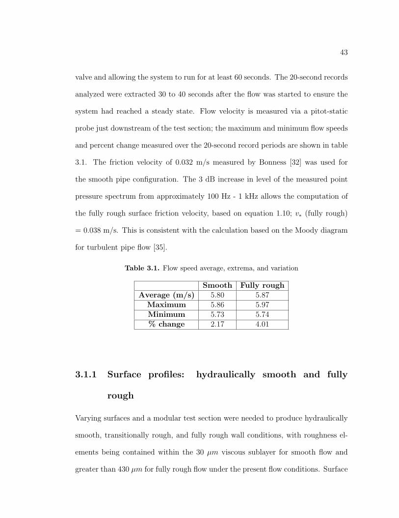
43

valve and allowing the system to run for at least 60 seconds. The 20-second records

analyzed were extracted 30 to 40 seconds after the flow was started to ensure the

system had reached a steady state. Flow velocity is measured via a pitot-static

probe just downstream of the test section; the maximum and minimum flow speeds

and percent change measured over the 20-second record periods are shown in table

3.1. The friction velocity of 0.032 m/s measured by Bonness [32] was used for

the smooth pipe configuration. The 3 dB increase in level of the measured point

pressure spectrum from approximately 100 Hz - 1 kHz allows the computation of

the fully rough surface friction velocity, based on equation 1.10; v∗ (fully rough)

= 0.038 m/s. This is consistent with the calculation based on the Moody diagram

for turbulent pipe flow [35].

Table 3.1. Flow speed average, extrema, and variation

Smooth Fully roughAverage (m/s) 5.80 5.87

Maximum 5.86 5.97Minimum 5.73 5.74% change 2.17 4.01

3.1.1 Surface profiles: hydraulically smooth and fully

rough

Varying surfaces and a modular test section were needed to produce hydraulically

smooth, transitionally rough, and fully rough wall conditions, with roughness el-

ements being contained within the 30 µm viscous sublayer for smooth flow and

greater than 430 µm for fully rough flow under the present flow conditions. Surface

44

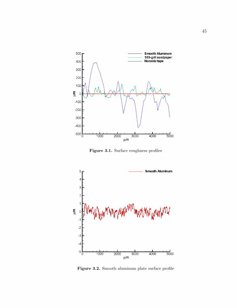
profiles of the smooth aluminum plate, 180-grit sandpaper, and nonskid tape are

shown for comparison in figure 3.1 and the smooth plate and nonskid tape are

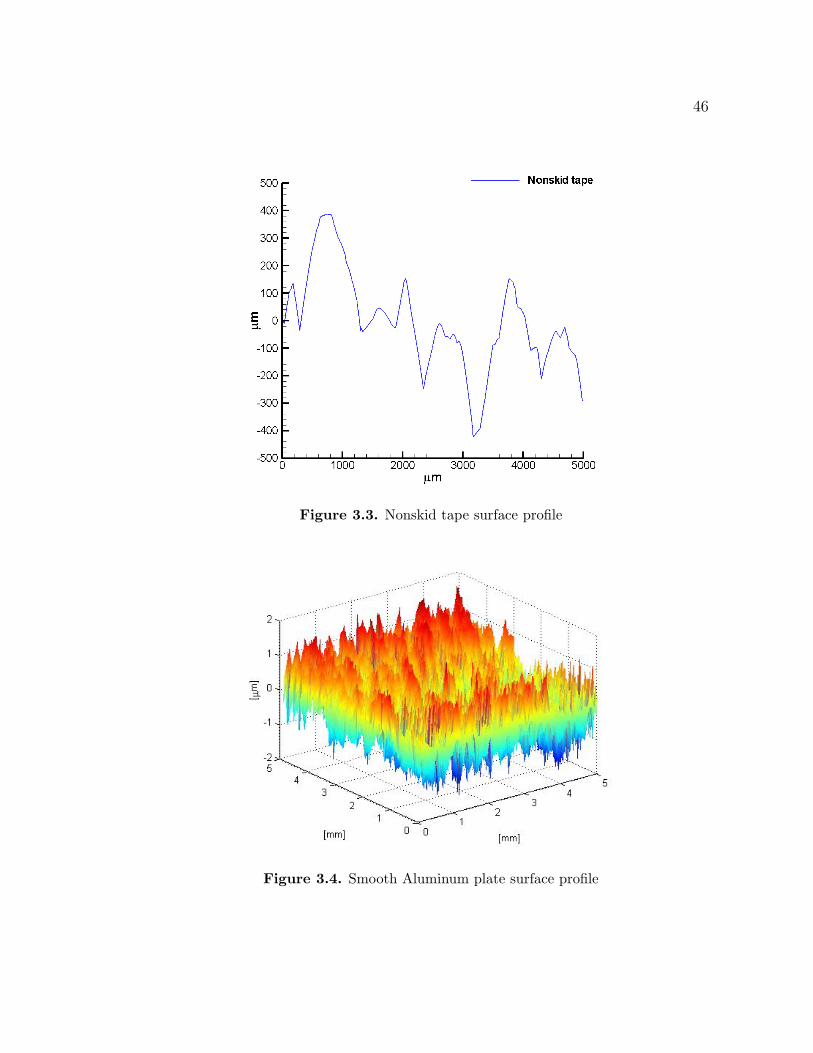
shown separately in figures 3.2 and 3.3. A typical measurement of the smooth

aluminum plate showed roughness elements of about 2µm peak-to-peak, and the

surface did not display a range greater than 4 µm peak-to-peak for any measure-

ment, keeping well within the viscous subrange. The nonskid tape has elements

greater than 800 µm peak-to-peak on the displayed measurement and exceeded

the profilometer’s 1 mm maximum excursion several times.

A number of adjacent traces were recorded of the smooth aluminum plate and

were combined to form a three-dimensional visualization of the surface, shown

in figure 3.4. Most measurements of the nonskid tape exceeded the 1 mm peak-

to-peak range of the profilometer, therefore a three-dimensional representation of

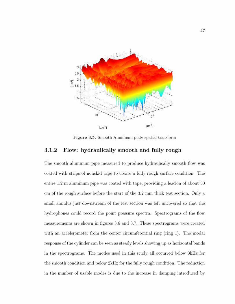
this surface could not be obtained. The spatial Fourier transform of the smooth

aluminum plate is shown in figure 3.5, where the mostly flat response indicates a

uniform surface and a wide distribution of element sizes.

45

Figure 3.1. Surface roughness profiles

Figure 3.2. Smooth aluminum plate surface profile

46

Figure 3.3. Nonskid tape surface profile

Figure 3.4. Smooth Aluminum plate surface profile

47

Figure 3.5. Smooth Aluminum plate spatial transform

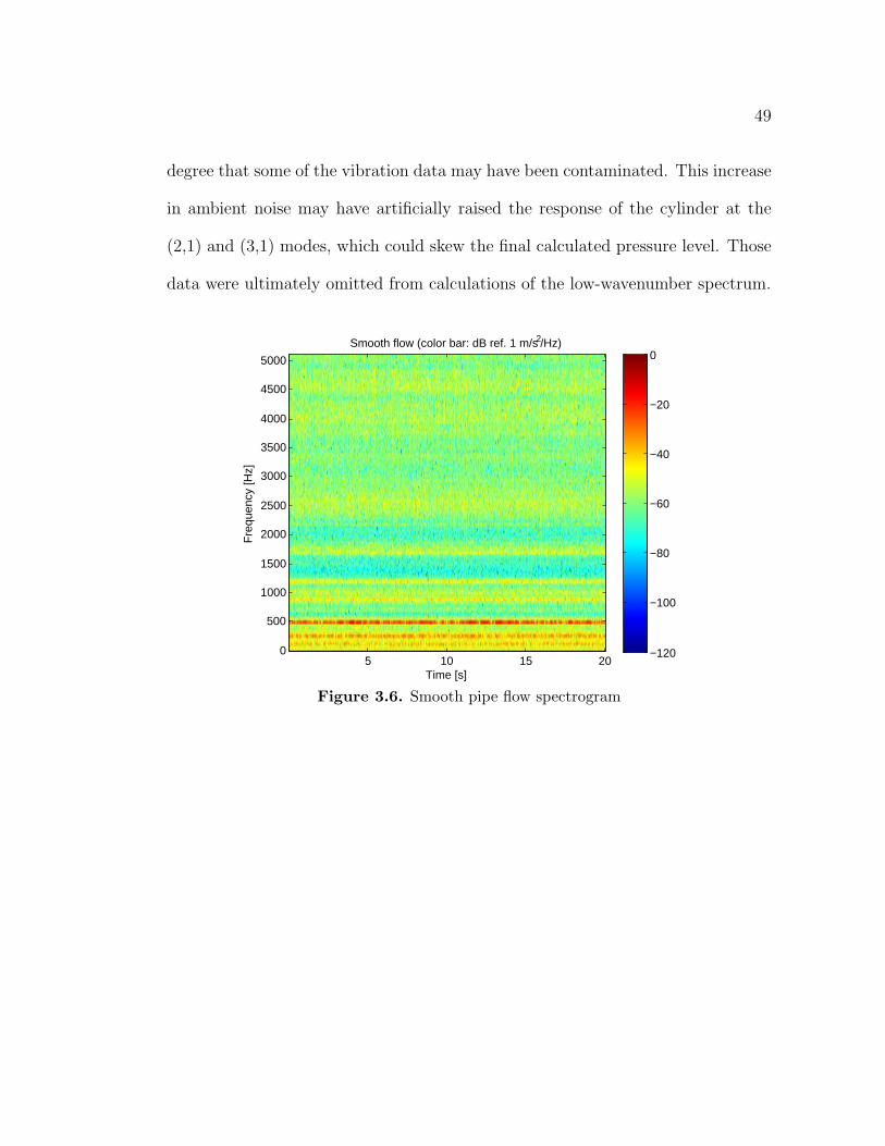
3.1.2 Flow: hydraulically smooth and fully rough

The smooth aluminum pipe measured to produce hydraulically smooth flow was

coated with strips of nonskid tape to create a fully rough surface condition. The

entire 1.2 m aluminum pipe was coated with tape, providing a lead-in of about 30

cm of the rough surface before the start of the 3.2 mm thick test section. Only a

small annulus just downstream of the test section was left uncovered so that the

hydrophones could record the point pressure spectra. Spectrograms of the flow

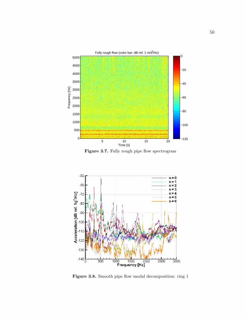
measurements are shown in figures 3.6 and 3.7. These spectrograms were created

with an accelerometer from the center circumferential ring (ring 1). The modal

response of the cylinder can be seen as steady levels showing up as horizontal bands

in the spectrograms. The modes used in this study all occurred below 3kHz for

the smooth condition and below 2kHz for the fully rough condition. The reduction

in the number of usable modes is due to the increase in damping introduced by

48

the nonskid tape and its adhesive onto the structure. The broadband transient

structures just visible at higher frequencies are the response of the accelerometer

to cavitation bursts within the pipe.

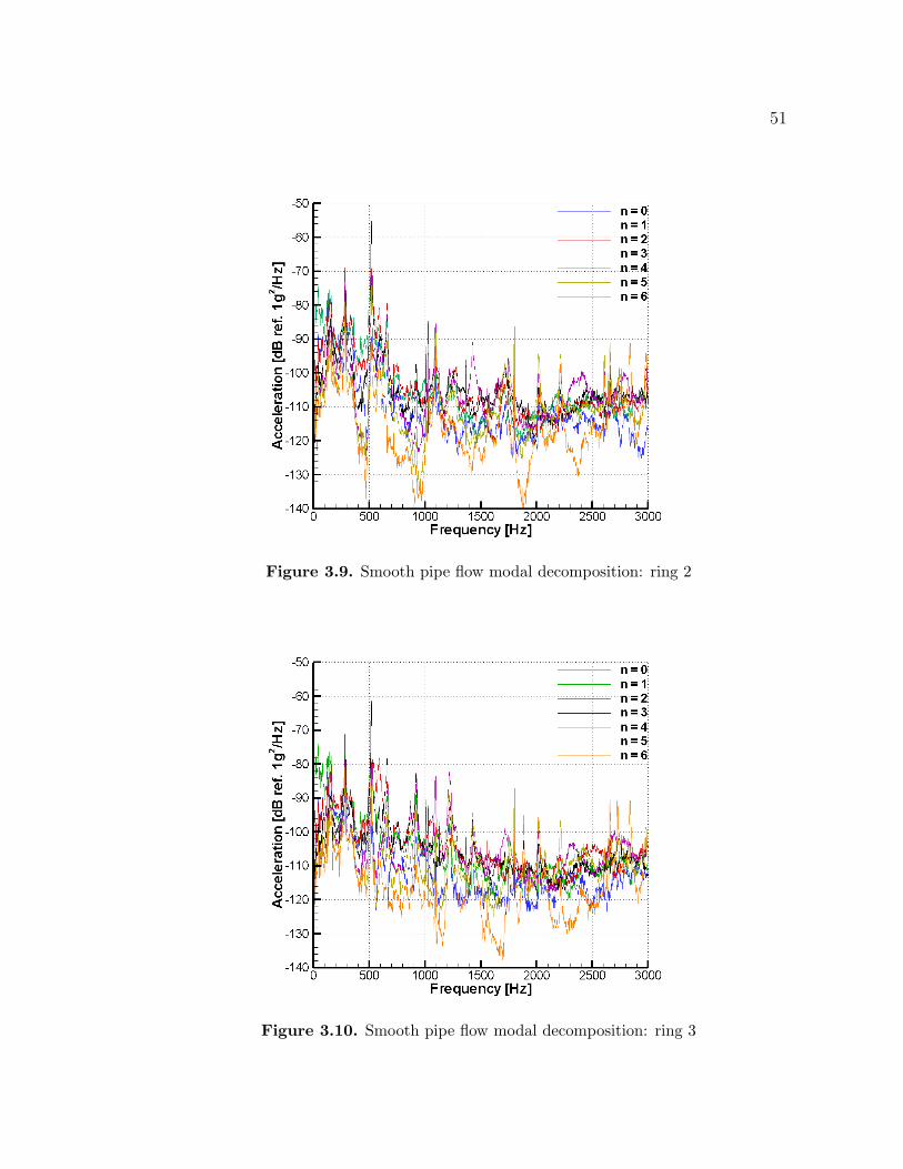
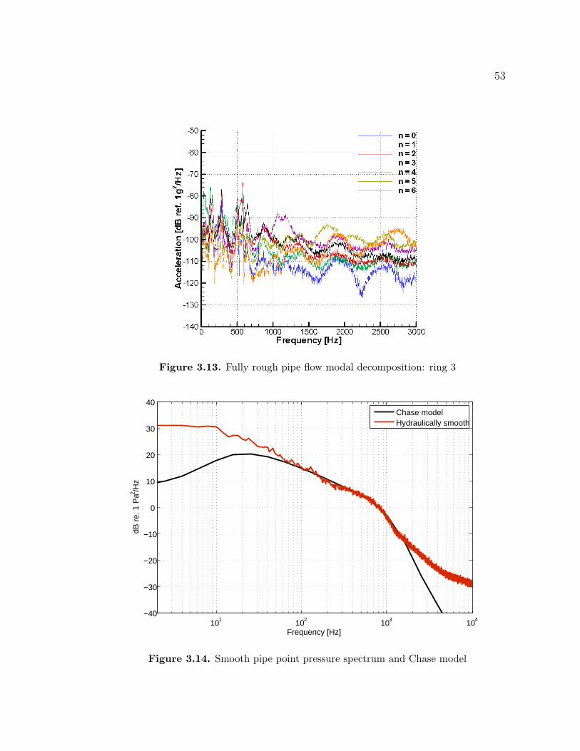
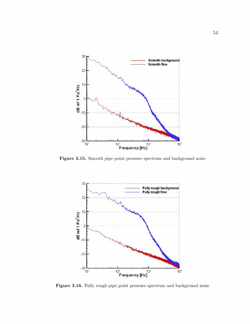
Circumferential modal decompositions of the aluminum cylindrical test sec-

tion’s vibration from the two flow conditions are shown in figures 3.8 - 3.13, where

n indicates the circumferential mode order. n = 0 is known as the breathing

mode and n = 1 is a translational mode; higher order modes, starting with n = 3

were used in the calculation of low-wavenumber pressures. The smooth wall point

pressure spectrum as measured by one hydrophone is shown in figure 3.14 along

with the point pressure spectrum of the 1987 Chase model [3], including the ef-

fects of transducer area averaging by Ko [5] and Lysak’s [21] decay due to viscous

effects. The measured point pressure spectrum matches the model well in the

mid-frequency range; high and low frequency ranges are limited by the noise floor

and by ambient vibration, respectively. The background noise during each of the

measurement periods is plotted along with the recorded spectra in figures 3.15 and

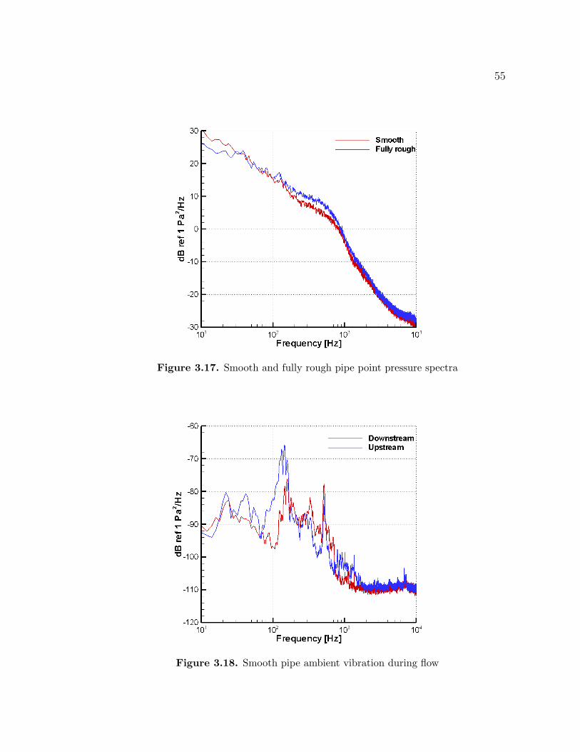
3.16. Figure 3.17 shows a comparison of the smooth and fully rough point pressure

spectra, where a slight increase in level is observed over the rough surface due to

increased turbulence production.

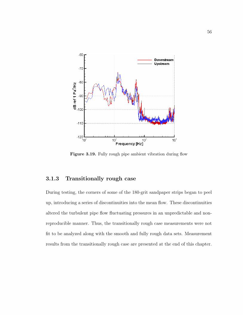
Ambient vibrational noise was measured by three upstream and three down-

stream accelerometers, attached to the structure supporting the test section and

oriented in each coordinate direction. Vibration measured perpendicular to the

floor, corresponding to an up and down translation of the system, is shown for the

smooth and fully rough cases in figures 3.18 and 3.19. The measured vibrational

noise displays an increase from about 100 - 600 Hz from an unknown source, to the

49

degree that some of the vibration data may have been contaminated. This increase

in ambient noise may have artificially raised the response of the cylinder at the

(2,1) and (3,1) modes, which could skew the final calculated pressure level. Those

data were ultimately omitted from calculations of the low-wavenumber spectrum.

Fre

quen

cy [H

z]

Time [s]

Smooth flow (color bar: dB ref. 1 m/s2/Hz)

5 10 15 200

500

1000

1500

2000

2500

3000

3500

4000

4500

5000

−120

−100

−80

−60

−40

−20

0

Figure 3.6. Smooth pipe flow spectrogram

50

Fre

quen

cy [H

z]

Time [s]

Fully rough flow (color bar: dB ref. 1 m/s2/Hz)

5 10 15 200

500

1000

1500

2000

2500

3000

3500

4000

4500

5000

−120

−100

−80

−60

−40

−20

0

Figure 3.7. Fully rough pipe flow spectrogram

Figure 3.8. Smooth pipe flow modal decomposition: ring 1

51

Figure 3.9. Smooth pipe flow modal decomposition: ring 2

Figure 3.10. Smooth pipe flow modal decomposition: ring 3

52

Figure 3.11. Fully rough pipe flow modal decomposition: ring 1

Figure 3.12. Fully rough pipe flow modal decomposition: ring 2

53

Figure 3.13. Fully rough pipe flow modal decomposition: ring 3

101 102 103 104−40

−30

−20

−10

0

10

20

30

40

Frequency [Hz]

dB r

e. 1

Pa2 /H

z

Chase modelHydraulically smooth

Figure 3.14. Smooth pipe point pressure spectrum and Chase model

54

Figure 3.15. Smooth pipe point pressure spectrum and background noise

Figure 3.16. Fully rough pipe point pressure spectrum and background noise

55

Figure 3.17. Smooth and fully rough pipe point pressure spectra

Figure 3.18. Smooth pipe ambient vibration during flow

56

Figure 3.19. Fully rough pipe ambient vibration during flow

3.1.3 Transitionally rough case

During testing, the corners of some of the 180-grit sandpaper strips began to peel

up, introducing a series of discontinuities into the mean flow. These discontinuities

altered the turbulent pipe flow fluctuating pressures in an unpredictable and non-

reproducible manner. Thus, the transitionally rough case measurements were not

fit to be analyzed along with the smooth and fully rough data sets. Measurement

results from the transitionally rough case are presented at the end of this chapter.

57

3.1.4 Modal analysis: hydraulically smooth and fully

rough

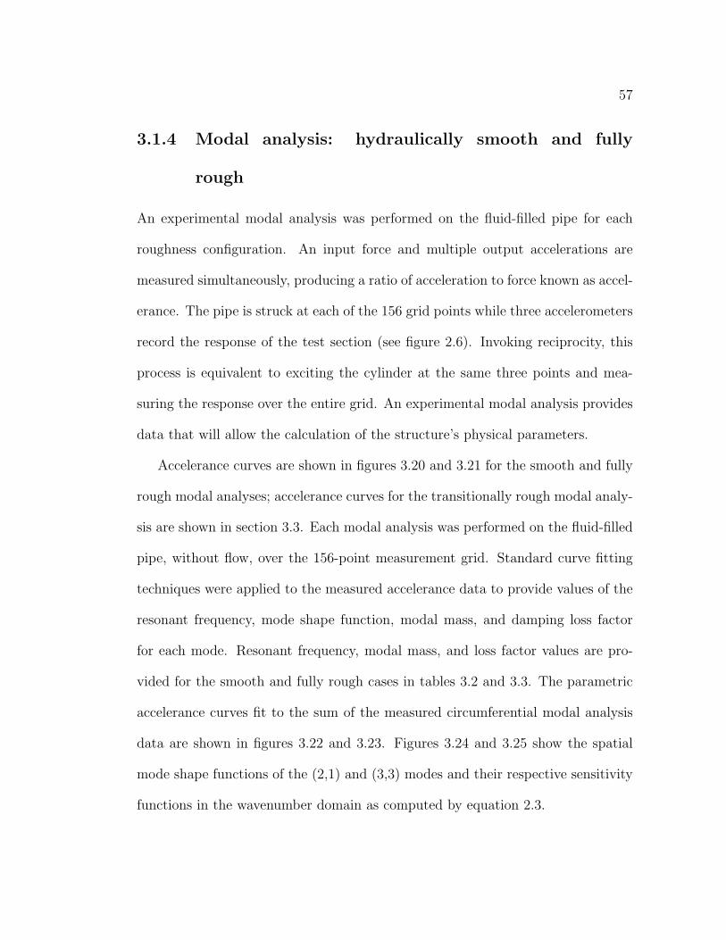
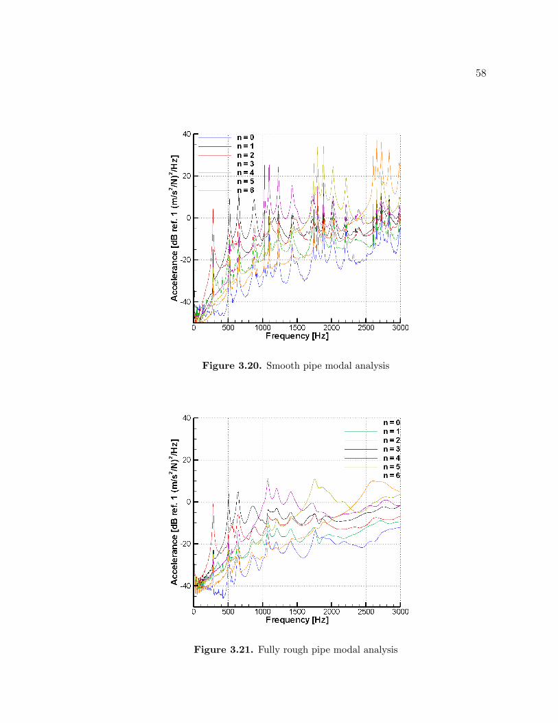
An experimental modal analysis was performed on the fluid-filled pipe for each

roughness configuration. An input force and multiple output accelerations are

measured simultaneously, producing a ratio of acceleration to force known as accel-

erance. The pipe is struck at each of the 156 grid points while three accelerometers

record the response of the test section (see figure 2.6). Invoking reciprocity, this

process is equivalent to exciting the cylinder at the same three points and mea-

suring the response over the entire grid. An experimental modal analysis provides

data that will allow the calculation of the structure’s physical parameters.

Accelerance curves are shown in figures 3.20 and 3.21 for the smooth and fully

rough modal analyses; accelerance curves for the transitionally rough modal analy-

sis are shown in section 3.3. Each modal analysis was performed on the fluid-filled

pipe, without flow, over the 156-point measurement grid. Standard curve fitting

techniques were applied to the measured accelerance data to provide values of the

resonant frequency, mode shape function, modal mass, and damping loss factor

for each mode. Resonant frequency, modal mass, and loss factor values are pro-

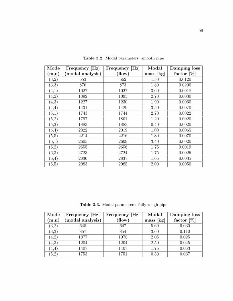
vided for the smooth and fully rough cases in tables 3.2 and 3.3. The parametric

accelerance curves fit to the sum of the measured circumferential modal analysis

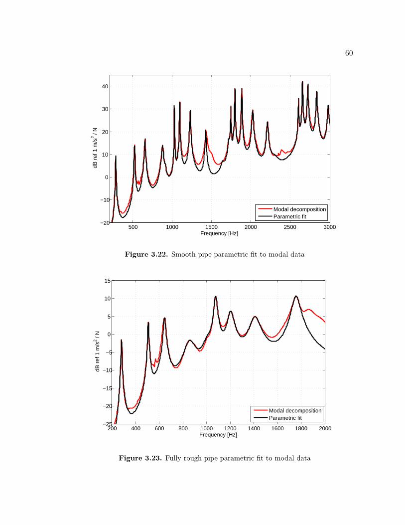
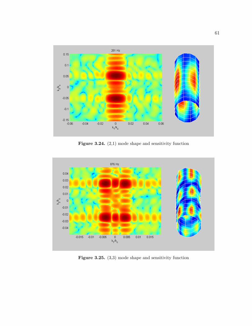
data are shown in figures 3.22 and 3.23. Figures 3.24 and 3.25 show the spatial

mode shape functions of the (2,1) and (3,3) modes and their respective sensitivity

functions in the wavenumber domain as computed by equation 2.3.

58

Figure 3.20. Smooth pipe modal analysis

Figure 3.21. Fully rough pipe modal analysis

59

Table 3.2. Modal parameters: smooth pipe

Mode Frequency [Hz] Frequency [Hz] Modal Damping loss(m,n) (modal analysis) (flow) mass [kg] factor [%](3,2) 653 662 1.30 0.0120(3,3) 876 873 1.80 0.0200(4,1) 1027 1027 3.60 0.0018(4,2) 1092 1093 2.70 0.0030(4,3) 1227 1230 1.90 0.0060(4,4) 1431 1429 3.50 0.0070(5,1) 1743 1744 2.70 0.0022(5,2) 1797 1801 1.20 0.0020(5,3) 1883 1883 0.40 0.0020(5,4) 2022 2019 1.00 0.0065(5,5) 2214 2216 1.80 0.0070(6,1) 2605 2609 3.40 0.0020(6,2) 2655 2656 1.75 0.0019(6,3) 2723 2724 1.75 0.0026(6,4) 2836 2837 1.65 0.0035(6,5) 2983 2985 2.00 0.0050

Table 3.3. Modal parameters: fully rough pipe

Mode Frequency [Hz] Frequency [Hz] Modal Damping loss(m,n) (modal analysis) (flow) mass [kg] factor [%](3,2) 645 647 5.60 0.030(3,3) 857 854 3.60 0.110(4,2) 1077 1078 2.05 0.025(4,3) 1204 1204 2.50 0.045(4,4) 1407 1407 1.75 0.063(5,2) 1753 1751 0.50 0.037

60

500 1000 1500 2000 2500 3000−20

−10

0

10

20

30

40

Frequency [Hz]

dB r

ef 1

m/s

2 / N

Modal decompositionParametric fit

Figure 3.22. Smooth pipe parametric fit to modal data

200 400 600 800 1000 1200 1400 1600 1800 2000−25

−20

−15

−10

−5

0

5

10

15

Frequency [Hz]

dB r

ef 1

m/s

2 / N

Modal decompositionParametric fit

Figure 3.23. Fully rough pipe parametric fit to modal data

61

Figure 3.24. (2,1) mode shape and sensitivity function

Figure 3.25. (3,3) mode shape and sensitivity function

62

3.2 Calculated low-wavenumber pressure levels

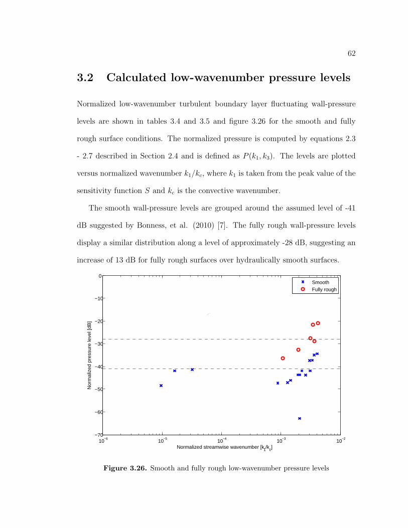
Normalized low-wavenumber turbulent boundary layer fluctuating wall-pressure

levels are shown in tables 3.4 and 3.5 and figure 3.26 for the smooth and fully

rough surface conditions. The normalized pressure is computed by equations 2.3

- 2.7 described in Section 2.4 and is defined as P (k1, k3). The levels are plotted

versus normalized wavenumber k1/kc, where k1 is taken from the peak value of the

sensitivity function S and kc is the convective wavenumber.

The smooth wall-pressure levels are grouped around the assumed level of -41

dB suggested by Bonness, et al. (2010) [7]. The fully rough wall-pressure levels

display a similar distribution along a level of approximately -28 dB, suggesting an

increase of 13 dB for fully rough surfaces over hydraulically smooth surfaces.

10−6

10−5

10−4

10−3

10−2

−70

−60

−50

−40

−30

−20

−10

0

Normalized streamwise wavenumber [k1/kc]

Nor

mal

ized

pre

ssur

e le

vel [

dB]

SmoothFully rough

Figure 3.26. Smooth and fully rough low-wavenumber pressure levels

63

Table 3.4. Smooth pipe low-wavenumber normalized pressure levels

Mode Normalized streamwise Normalized pressure(m,n) wavenumber [1000k1/kc] level [dB](3,2) 3.401 -35(3,3) 4.105 -35(4,1) 0.016 -43(4,2) 2.095 -44(4,3) 3.094 -43(4,4) 3.629 -35(5,1) 0.010 -46(5,2) 1.294 -48(5,3) 2.070 -61(5,4) 2.622 -44(5,5) 3.035 -36(6,1) 0.032 -41(6,2) 0.888 -47(6,3) 1.456 -46(6,4) 1.905 -44(6,5) 2.249 -42

Table 3.5. Fully rough pipe low-wavenumber normalized pressure levels

Mode Normalized streamwise Normalized pressure(m,n) wavenumber [1000k1/kc] level [dB](3,2) 3.436 -23(3,3) 4.209 -21(4,2) 1.965 -33(4,3) 3.164 -28(4,4) 3.691 -29(5,2) 1.071 -36

3.3 Transitionally rough case

3.3.1 Surface profile

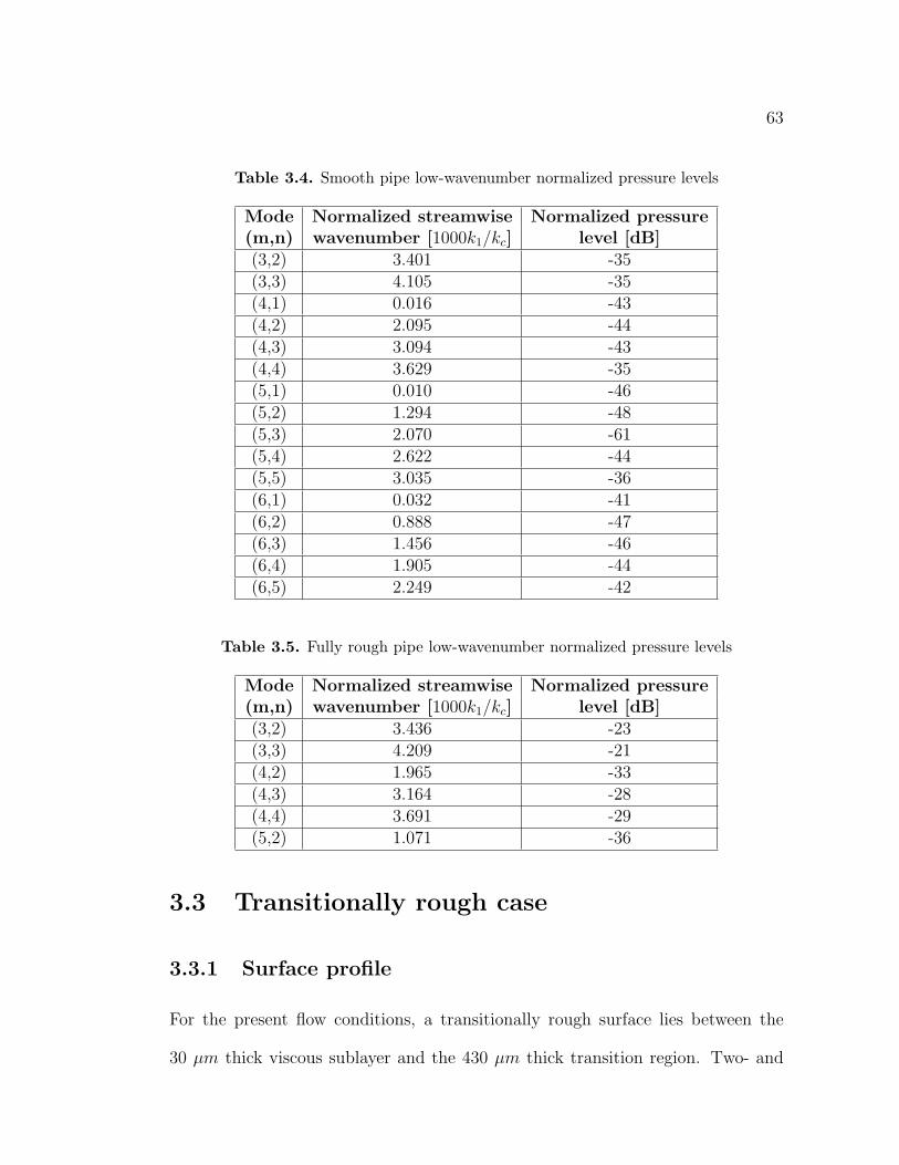
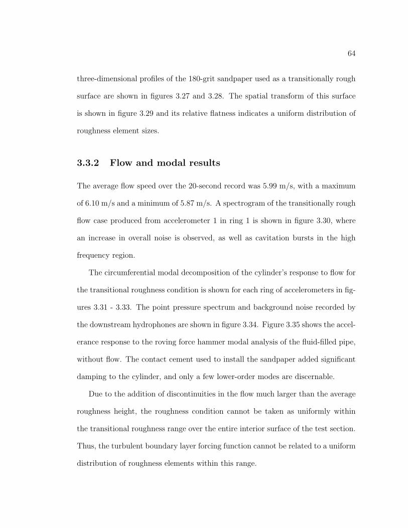
For the present flow conditions, a transitionally rough surface lies between the

30 µm thick viscous sublayer and the 430 µm thick transition region. Two- and

64

three-dimensional profiles of the 180-grit sandpaper used as a transitionally rough

surface are shown in figures 3.27 and 3.28. The spatial transform of this surface

is shown in figure 3.29 and its relative flatness indicates a uniform distribution of

roughness element sizes.

3.3.2 Flow and modal results

The average flow speed over the 20-second record was 5.99 m/s, with a maximum

of 6.10 m/s and a minimum of 5.87 m/s. A spectrogram of the transitionally rough

flow case produced from accelerometer 1 in ring 1 is shown in figure 3.30, where

an increase in overall noise is observed, as well as cavitation bursts in the high

frequency region.

The circumferential modal decomposition of the cylinder’s response to flow for

the transitional roughness condition is shown for each ring of accelerometers in fig-

ures 3.31 - 3.33. The point pressure spectrum and background noise recorded by

the downstream hydrophones are shown in figure 3.34. Figure 3.35 shows the accel-

erance response to the roving force hammer modal analysis of the fluid-filled pipe,

without flow. The contact cement used to install the sandpaper added significant

damping to the cylinder, and only a few lower-order modes are discernable.

Due to the addition of discontinuities in the flow much larger than the average

roughness height, the roughness condition cannot be taken as uniformly within

the transitional roughness range over the entire interior surface of the test section.

Thus, the turbulent boundary layer forcing function cannot be related to a uniform

distribution of roughness elements within this range.

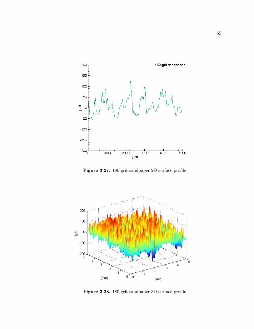
65

Figure 3.27. 180-grit sandpaper 2D surface profile

Figure 3.28. 180-grit sandpaper 3D surface profile

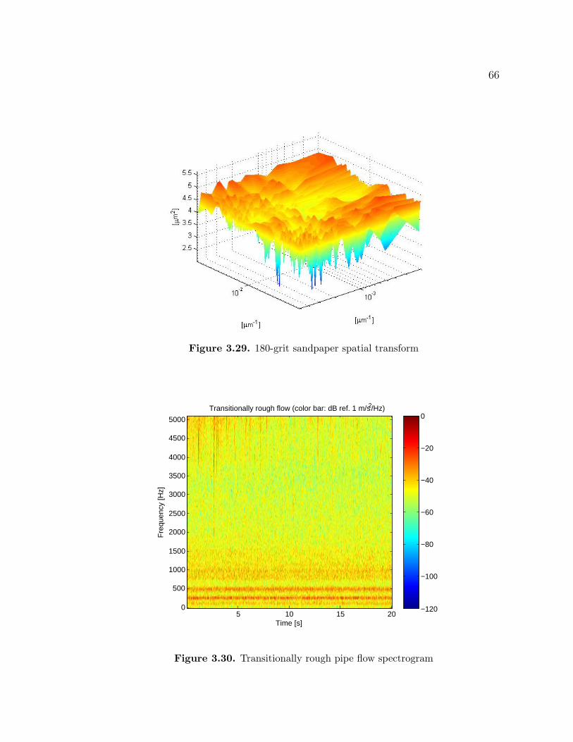
66

Figure 3.29. 180-grit sandpaper spatial transform

Fre

quen

cy [H

z]

Time [s]

Transitionally rough flow (color bar: dB ref. 1 m/s2/Hz)

5 10 15 200

500

1000

1500

2000

2500

3000

3500

4000

4500

5000

−120

−100

−80

−60

−40

−20

0

Figure 3.30. Transitionally rough pipe flow spectrogram

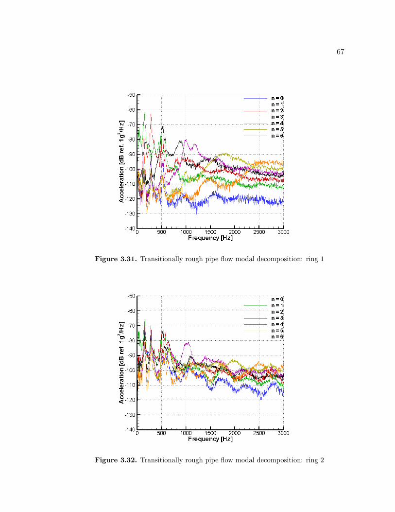
67

Figure 3.31. Transitionally rough pipe flow modal decomposition: ring 1

Figure 3.32. Transitionally rough pipe flow modal decomposition: ring 2

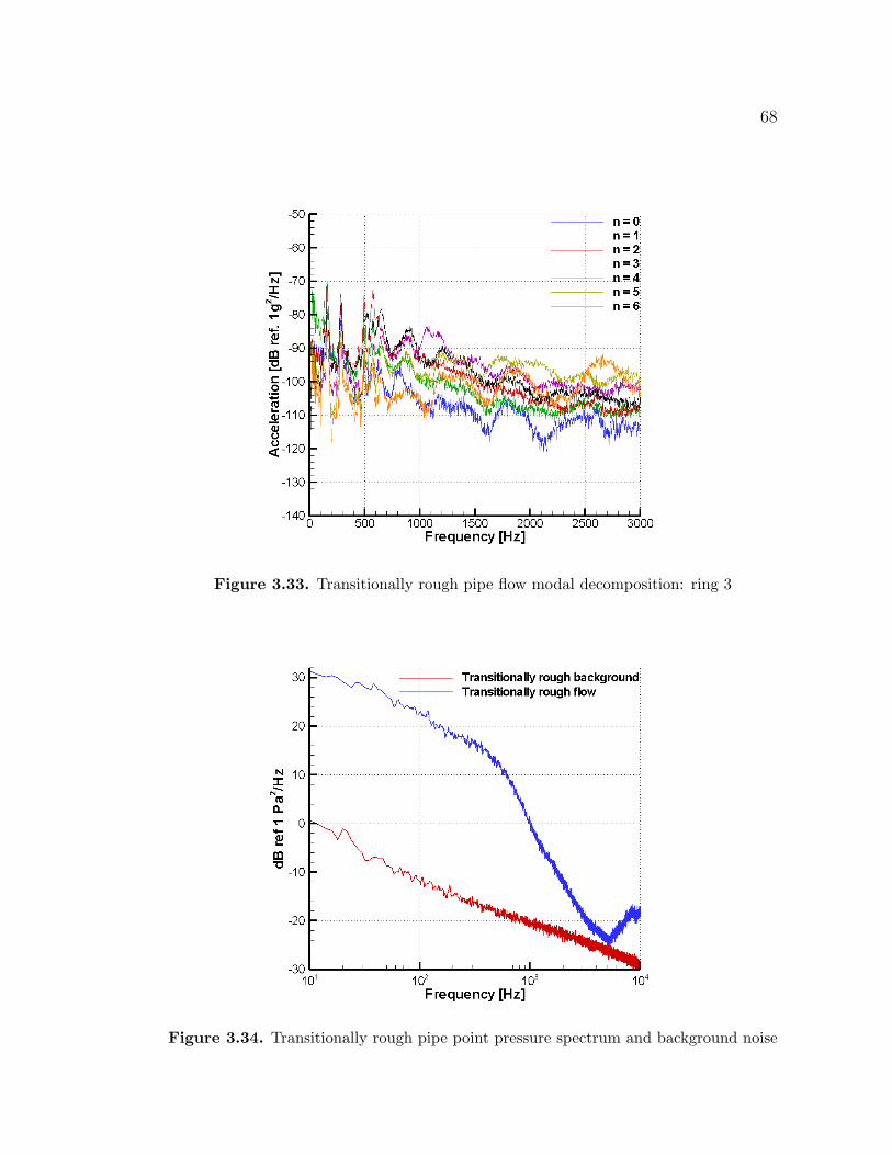
68

Figure 3.33. Transitionally rough pipe flow modal decomposition: ring 3

Figure 3.34. Transitionally rough pipe point pressure spectrum and background noise

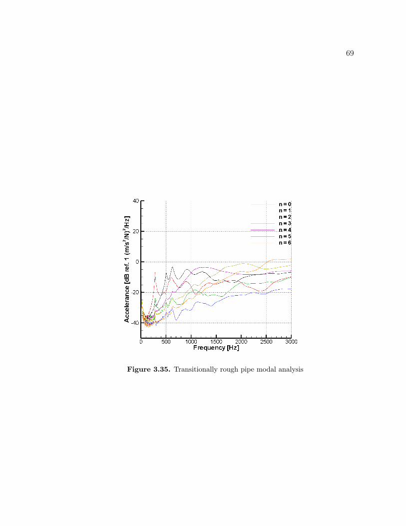
69

Figure 3.35. Transitionally rough pipe modal analysis

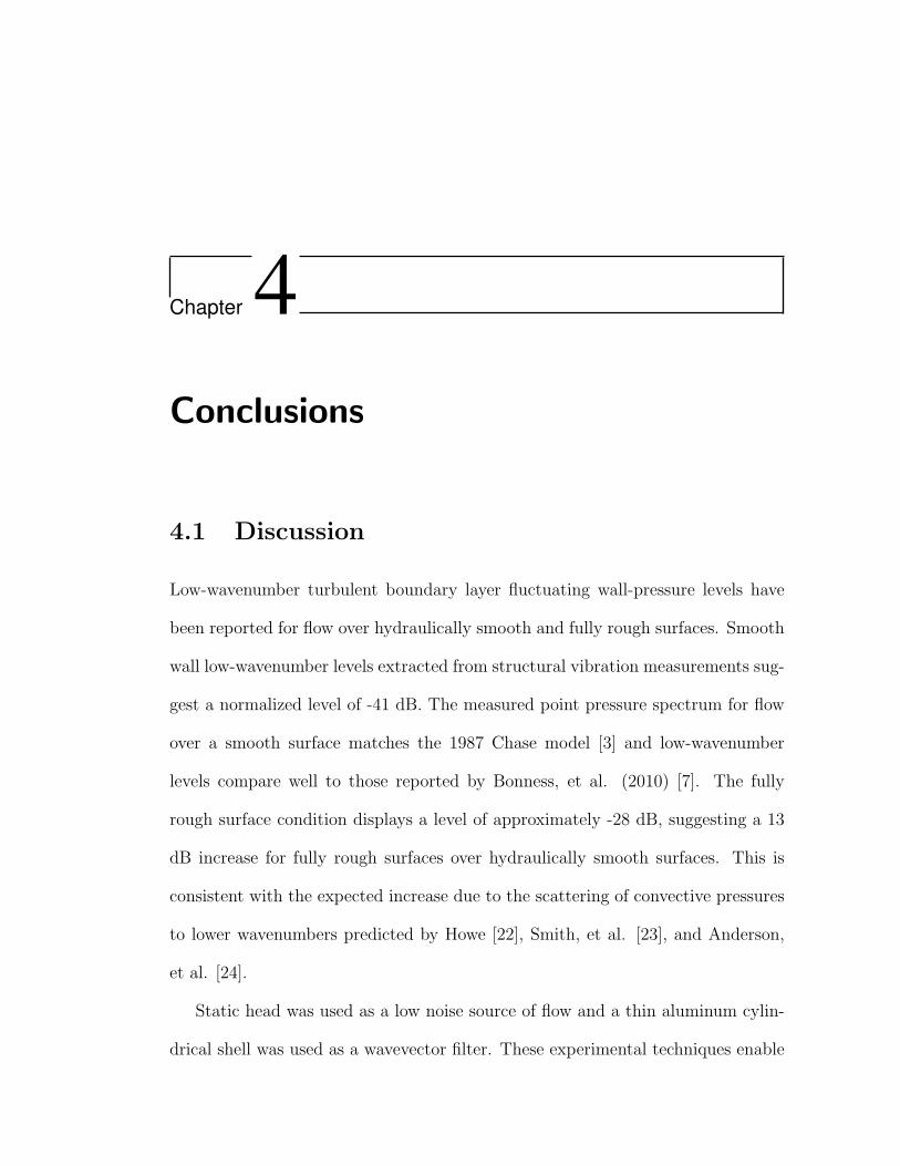
Chapter 4Conclusions

4.1 Discussion

Low-wavenumber turbulent boundary layer fluctuating wall-pressure levels have

been reported for flow over hydraulically smooth and fully rough surfaces. Smooth

wall low-wavenumber levels extracted from structural vibration measurements sug-

gest a normalized level of -41 dB. The measured point pressure spectrum for flow

over a smooth surface matches the 1987 Chase model [3] and low-wavenumber

levels compare well to those reported by Bonness, et al. (2010) [7]. The fully

rough surface condition displays a level of approximately -28 dB, suggesting a 13

dB increase for fully rough surfaces over hydraulically smooth surfaces. This is

consistent with the expected increase due to the scattering of convective pressures

to lower wavenumbers predicted by Howe [22], Smith, et al. [23], and Anderson,

et al. [24].

Static head was used as a low noise source of flow and a thin aluminum cylin-

drical shell was used as a wavevector filter. These experimental techniques enable

71

the measurement of the low-wavenumber region of the turbulent boundary layer

pressure spectrum which is otherwise difficult to extract due to masking by convec-

tive pressures. The experiment may have some limitations, however. The use of

a spatial filter is necessary in the extraction of low-wavenumber, long wavelength

pressures which are difficult to measure directly but couple well to structures. Us-

ing a structural wavevector filter provides pressure levels at a few discrete points,

related to structural resonances, and not as a continuous spectrum. Thus, the

actual form of the spectrum must be inferred from these observed discrete points.

As more data describing the low-wavenumber region come forth, the form of the

turbulent boundary layer pressure spectrum is pieced together and extended to

lower wavenumbers and additional surface conditions.

Even when care is taken, it is difficult to create a turbulent flow system without

any discontinuities or unintended surface roughness elements, both of which im-

pact the structure of the turbulent boundary layer and the pressures it produces.

For example, the interior surface of a wind tunnel or piping system may not be

uniformly hydraulically smooth, or pipe segments may not have perfectly flush

joints.

The use of static head to drive flow through the test apparatus decreases facility

noise considerably over a wind or water tunnel experiment, but background noise

from sources such as nearby road traffic and other facility operations is still present.

Low-wavenumber pressures by nature must be measured inversely and care must

be taken to minimize background noise. A valid experiment must optimize a given

scenario to ensure its validity.

Despite any inherent difficulties, the present experiment has provided measure-

72

ments of low-wavenumber pressure levels down to normalized streamwise wavenum-

bers k1/kc of the order 10−5 for smooth conditions and 10−3 for fully rough condi-

tions. These wavenumbers are lower than previously reported data for fully rough

conditions. The fully rough levels track the hydraulically smooth levels well, and

suggest a 13 dB correction factor.

4.2 Suggestions for future work

Future experiments may be implemented to quantify the low-wavenumber effects

of larger, discrete surface roughness elements and discontinuities, to augment the

study of uniformly distributed roughness elements investigated here. Measure-

ments of a transitionally rough surface could be revisited, which may show a spec-

tral level somewhere between hydraulically smooth and fully rough surfaces.

The addition of sandpaper and nonskid tape as forms of surface roughness

introduced damping into the system, and thus fewer modes were resolved for the

rough condition. It would be ideal if the damping were unchanged between the

smooth and rough conditions and a one to one comparison of every mode could be

made. Alternate methods of roughening the aluminum surface were investigated,

such as abrasing the surface or allowing it to corrode, however these methods did

not produce the desired degree of roughness and may not have been uniform over

the entire pipe interior. A future option for creating roughness that does not add

damping to the structure could involve machining a series of holes or grooves of

various sizes and depths into the surface.

The present data should be incorporated in the refinement of the low-

73

wavenumber region of turbulent boundary layer models, which were developed

before adequate low-wavenumber data were available and are primarily concerned

with smooth surfaces. Alternatively, a new model could be developed that accu-

rately reflects both the well-described convective region and the recently measured

low-wavenumber region. Until a full theory of turbulence is produced, parametric

models motivated by experiments will continue to prevail, and it is through the

incremental work of experimentalists that such knowledge of the structure of the

turbulent boundary layer will be advanced.

Bibliography

[1] Skudrzyk, E. J. and G. P. Haddle (1958) “Noise production in a turbu-lent boundary layer by smooth and rough surfaces,” Journal of the AcousticalSociety of America, 32(1), pp. 19–34.

[2] Corcos, G. M. (1963) “Resolution of pressure in turbulence,” Journal ofthe Acoustical Society of America, 35(2), pp. 192–199.

[3] Chase, D. M. (1987) “The character of the turbulent wall pressure at sub-convective wavenumbers and a suggested comprehensive model,” Journal ofSound and Vibration, 112(1), pp. 125–147.

[4] Smol’yakov, A. V. (2000) “Calculation of the spectra of pseudosound wall-pressure fluctuations in turbulent boundary layers,” Acoustical Physics, 46(3),pp. 401–407.

[5] Ko, S. H. (1993) “Performance of various shapes of hydrophones in the re-duction of turbulent flow noise,” Journal of the Acoustical Society of America,93(3), pp. 1041–1047.

[6] Bull, M. K. (1967) “Wall-pressure fluctuations associated with subsonicturbulent boundary layer flow,” Journal of Fluid Mechanics, 28(4), pp. 719–754.

[7] Bonness, W. K., D. E. Capone, and S. A. Hambric (2010) “Low-wavenumber turbulent boundary layer wall-pressure measurements from vi-bration data on a cylinder in pipe flow,” Journal of Sound and Vibration,329, pp. 4166–4180.

[8] Fox, R. W., A. T. McDonald, and P. J. Pritchard (2004) Introductionto Fluid Mechanics, ‘Wiley’.

[9] Schlichting, H. (1987) Boundary Layer Theory, 7th ed., ‘McGraw-Hill’.

75

[10] Kirsten, H. (1927) Experimentelle untersuchungen der entwicklungder geschwindigkeitsverteilung der turbulenten rohrstromung, Ph.D. thesis,Leipzig.

[11] Nikuradse, J. (1932) “Gesetzmassigkeit der turbulenten stromung in glattenrohren,” Forschg. Arb. Ing.-Wes., (356).

[12] Farabee, T. M. and F. E. Geib Jr. (1991) “Measurements of boundarylayer pressure fluctuations at low wavenumbers on smooth and rough walls,”Flow Noise Modeling, Measurement, and Control, 11(H00713).

[13] Blake, W. K. (1970) “Turbulent boundary-layer wall-pressure fluctuationson smooth and rough walls,” Journal of Fluid Mechanics, 44(4), pp. 637–659.

[14] Willmarth, W. W. and C. E. Woolridge (1962) “Measurements of thefluctuating pressure at the wall beneath a thick turbulent boundary layer,”Journal of Fluid Mechanics, 14(2), pp. 187–210.

[15] Maidanik, G. and T. Eisler (1982) “Reasons and means for measuringthe spectral density of the pressure in a subsonic turbulent boundary layer,”Journal of Sound and Vibration, 84(3), pp. 397–416.

[16] Martin, N. C. and P. Leehey (1977) “Low wavenumber wall pressuremeasurements using a rectangular membrane as a spatial filter,” Journal ofSound and Vibration, 52(1), pp. 95–120.

[17] Panton, R. L., A. L. Goldman, R. L. Lowery, and M. M. Reis-chman (1980) “Low-frequency pressure fluctuations in axisymmetric turbu-lent boundary layers,” Journal of Fluid Mechanics, 97(2), pp. 299–319.

[18] Farabee, T. M. and F. E. Geib Jr. (1975) “Measurement of boundarylayer pressure fields with an array of pressure transducers in subsonic flow,”ICIASF ’75 Record, pp. 311–319.

[19] Chase, D. M. (1980) “Modeling the wavevector-frequency spectrum of tur-bulent boundary layer wall pressure,” Journal of Sound and Vibration, 70(1),pp. 29–67.

[20] Howe, M. S. (1979) “The role of surface shear stress fluctuations in thegeneration of boundary layer noise,” Journal of Sound and Vibration, 65(2),pp. 159–164.

[21] Lysak, P. D. (2006) “Modeling the wall pressure spectrum in turbulent pipeflows,” Transactions of the ASME, 128, pp. 216–222.

76

[22] Howe, M. S. (1991) “Surface pressures and sound produced by turbulent flowover smooth and rough walls,” Journal of the Acoustical Society of America,90(2), pp. 1041–1047.

[23] Smith, B. S., W. N. Alexander, W. Devenport, S. A. L. Glegg,and D. L. Grissom (May 2008) “The relationship between roughness noiseand the near-field pressure spectrum (AIAA paper no. 2008-2904),” 14thAIAA/CEAS Aeroacoustics Conference (29th AIAA Aeroacoustics Confer-ence), Vancouver, British Columbia Canada.

[24] Anderson, J. M., D. O. Stewart, and W. K. Blake (November 2009)“Experimental investigations of sound from flow over rough surfaces,” Pro-ceedings of the ASME 2009 International Mechanical Engineering Congressand Exposition, Lake Buena Vista, Florida, USA.

[25] Glegg, S. and W. Devenport (2009) “The far-field sound from rough-wallboundary layers,” Proceedings of the Royal Society, 465, pp. 1717–1734.

[26] Antonia, R. A. and R. E. Luxton (1971) “The response of a turbu-lent boundary layer to a step change in surface roughness Part 1. Smooth torough,” Journal of Fluid Mechanics, 48(4), pp. 721–761.

[27] Antonia, R. A. and R. Luxton (1971) “The response of a turbulent bound-ary layer to an upstanding step change in surface roughness,” Transaction ofthe ASME, pp. 22–32.

[28] Cheng, H. and I. P. Castro (2002) “Near-wall flow development aftera step change in surface roughness,” Boundary-Layer Meteorology, 105, pp.411–432.

[29] Laws, E. M. (1990) “Flow conditioning - a new development,” Flow Mea-surement Instrumentation, 1, pp. 165–170.

[30] Hwang, Y. F. and G. Maidanik (1990) “A wavenumber analysis of thecoupling of a structural mode and flow turbulence,” Journal of Sound andVibration, 142(1), pp. 135–152.

[31] Ewins, D. J. (1984) Modal Testing: Theory and Practice, ‘Research StudiesPress Ltd.’.

[32] Bonness, W. K. (2009) Low wavenumber turbulent boundary layer wall pres-sure and shear stress measurements from vibration data on a cylinder in pipeflow, Ph.D. thesis, The Pennsylvania State University, State College, Penn-sylvania.

77

[33] Gabrielson, T. (2010), “Course Notes: ACS 516, Acoustical Data Mea-surement and Analysis,” The Pennsylvania State University.

[34] Bendat, J. S. and A. G. Piersol (1986) Random Data Analysis and Mea-surement Procedures, ‘Wiley-Interscience’.

[35] Cengel, Y. A. and J. M. Cimbala (2006) Fluid Mechanics: Fundamentalsand applications, ‘McGraw-Hill’.