The New Keynesian Model - SSCC - Home

The New Keynesian Model

Noah Williams

University of Wisconsin-Madison

Noah Williams (UW Madison) New Keynesian model 1 / 51

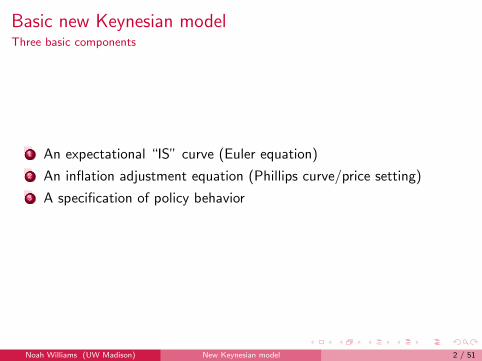
Basic new Keynesian modelThree basic components

1 An expectational “IS” curve (Euler equation)

2 An inflation adjustment equation (Phillips curve/price setting)

3 A specification of policy behavior


Overview of the Model

The model consists of households who supply labor, purchase goodsfor consumption, and hold money and bonds, and firms who hirelabor and produce and sell differentiated products in monopolisticallycompetitive goods markets.

The basic model of monopolistic competition is drawn from Dixit andStiglitz (1977).

Each firm set the price of the good it produces, but not all firms resettheir price each period.

Households and firms behave optimally: households maximize theexpected present value of utility and firms maximize profits.


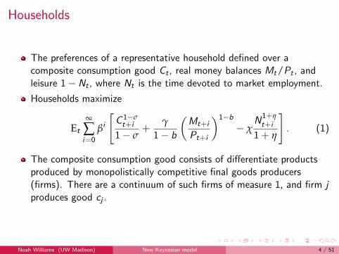
Households

The preferences of a representative household defined over acomposite consumption good Ct , real money balances Mt/Pt , andleisure 1−Nt , where Nt is the time devoted to market employment.

Households maximize

Et

∞

∑i=0

βi

[C 1−σt+i

1− σ+

γ

1− b

(Mt+i

Pt+i

)1−b− χ

N1+ηt+i

1 + η

]. (1)

The composite consumption good consists of differentiate productsproduced by monopolistically competitive final goods producers(firms). There are a continuum of such firms of measure 1, and firm jproduces good cj .


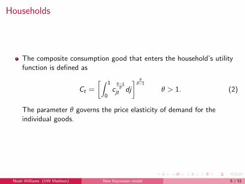
Households

The composite consumption good that enters the household’s utilityfunction is defined as

Ct =

[∫ 1

0c

θ−1θ

jt dj

] θθ−1

θ > 1. (2)

The parameter θ governs the price elasticity of demand for theindividual goods.


Households

The household’s decision problem can be dealt with in two stages.

1 Regardless of the level of Ct , it will always be optimal to purchase thecombination of the individual goods that minimize the cost ofachieving this level of the composite good.

2 Given the cost of achieving any given level of Ct , the householdchooses Ct , Nt , and Mt optimally.


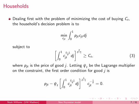
Households

Dealing first with the problem of minimizing the cost of buying Ct ,the household’s decision problem is to

mincjt

∫ 1

0pjtcjtdj

subject to [∫ 1

0c

θ−1θ

jt dj

] θθ−1≥ Ct , (3)

where pjt is the price of good j . Letting ψt be the Lagrange multiplieron the constraint, the first order condition for good j is

pjt − ψt

[∫ 1

0c

θ−1θ

jt dj

] 1θ−1

c− 1

θjt = 0.


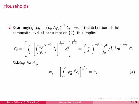
Households

Rearranging, cjt = (pjt/ψt)−θ Ct . From the definition of the

composite level of consumption (2), this implies

Ct =

∫ 1

0

[(pjtψt

)−θ

Ct

] θ−1θ

dj

θ

θ−1

=

(1

ψt

)−θ [∫ 1

0p1−θjt dj

] θθ−1

Ct .

Solving for ψt ,

ψt =

[∫ 1

0p1−θjt dj

] 11−θ

≡ Pt . (4)


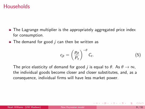
Households

The Lagrange multiplier is the appropriately aggregated price indexfor consumption.

The demand for good j can then be written as

cjt =

(pjtPt

)−θ

Ct . (5)

The price elasticity of demand for good j is equal to θ. As θ → ∞,the individual goods become closer and closer substitutes, and, as aconsequence, individual firms will have less market power.


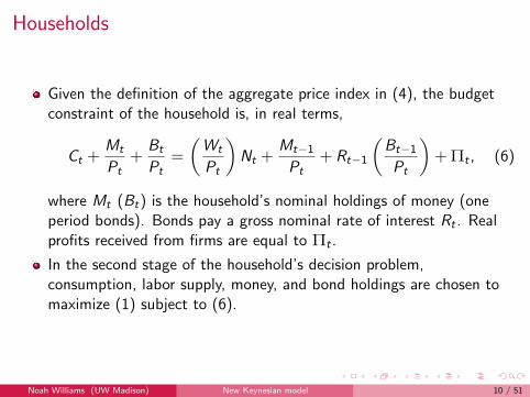
Households

Given the definition of the aggregate price index in (4), the budgetconstraint of the household is, in real terms,

Ct +Mt

Pt+

Bt

Pt=

(Wt

Pt

)Nt +

Mt−1Pt

+ Rt−1

(Bt−1Pt

)+ Πt , (6)

where Mt (Bt) is the household’s nominal holdings of money (oneperiod bonds). Bonds pay a gross nominal rate of interest Rt . Realprofits received from firms are equal to Πt .

In the second stage of the household’s decision problem,consumption, labor supply, money, and bond holdings are chosen tomaximize (1) subject to (6).


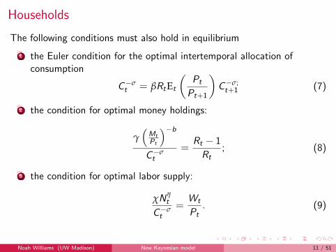
Households

The following conditions must also hold in equilibrium

1 the Euler condition for the optimal intertemporal allocation ofconsumption

C−σt = βRtEt

(Pt

Pt+1

)C−σ;t+1 (7)

2 the condition for optimal money holdings:

γ(MtPt

)−bC−σt

=Rt − 1

Rt; (8)

3 the condition for optimal labor supply:

χNηt

C−σt

=Wt

Pt. (9)


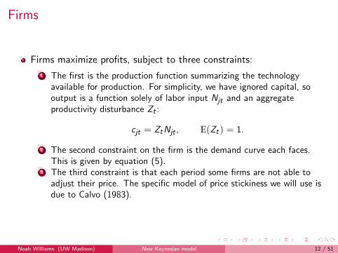
Firms

Firms maximize profits, subject to three constraints:

1 The first is the production function summarizing the technologyavailable for production. For simplicity, we have ignored capital, sooutput is a function solely of labor input Njt and an aggregateproductivity disturbance Zt :

cjt = ZtNjt , E(Zt) = 1.

2 The second constraint on the firm is the demand curve each faces.This is given by equation (5).

3 The third constraint is that each period some firms are not able toadjust their price. The specific model of price stickiness we will use isdue to Calvo (1983).


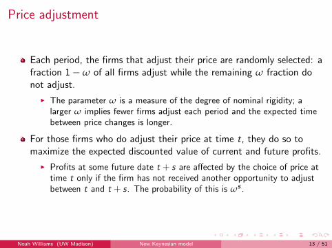
Price adjustment

Each period, the firms that adjust their price are randomly selected: afraction 1−ω of all firms adjust while the remaining ω fraction donot adjust.

I The parameter ω is a measure of the degree of nominal rigidity; alarger ω implies fewer firms adjust each period and the expected timebetween price changes is longer.

For those firms who do adjust their price at time t, they do so tomaximize the expected discounted value of current and future profits.

I Profits at some future date t + s are affected by the choice of price attime t only if the firm has not received another opportunity to adjustbetween t and t + s. The probability of this is ωs .


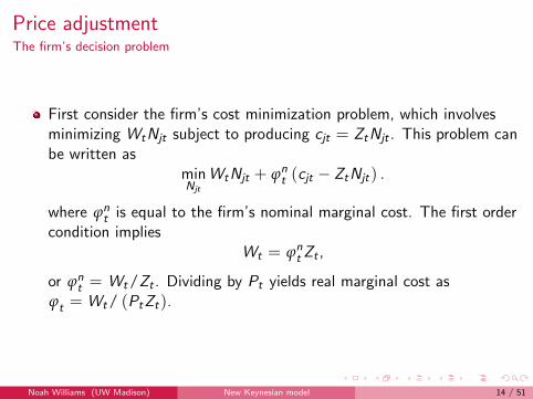
Price adjustmentThe firm’s decision problem

First consider the firm’s cost minimization problem, which involvesminimizing WtNjt subject to producing cjt = ZtNjt . This problem canbe written as

minNjt

WtNjt + ϕnt (cjt − ZtNjt) .

where ϕnt is equal to the firm’s nominal marginal cost. The first order

condition impliesWt = ϕn

tZt ,

or ϕnt = Wt/Zt . Dividing by Pt yields real marginal cost as

ϕt = Wt/ (PtZt).


Price adjustmentThe firm’s decision problem

The firm’s pricing decision problem then involves picking pjt tomaximize

Et

∞

∑i=0

ωi∆i ,t+iΠ(

pjtPt+i

, ϕt+i , ct+i

)=

Et

∞

∑i=0

ωi∆i ,t+i

[(pjtPt+i

)1−θ

− ϕt+i

(pjtPt+i

)−θ]Ct+i ,

where the discount factor ∆i ,t+i is given by βi (Ct+i/Ct)−σ andprofits are

Π(pjt) =

[(pjtPt+i

)cjt+i − ϕt+icjt+i

]


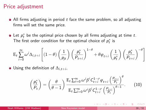
Price adjustment

All firms adjusting in period t face the same problem, so all adjustingfirms will set the same price.

Let p∗t be the optimal price chosen by all firms adjusting at time t.The first order condition for the optimal choice of p∗t is

Et

∞

∑i=0

ωi∆i ,t+i

[(1− θ)

(1

pjt

)(p∗tPt+i

)1−θ

+ θϕt+i

(1

p∗t

)(p∗tPt+i

)−θ]Ct+i = 0.

Using the definition of ∆i ,t+i ,

(p∗tPt

)=

(θ

θ − 1

) Et ∑∞i=0 ωi βiC 1−σ

t+i ϕt+i

(Pt+i

Pt

)θ

Et ∑∞i=0 ωi βiC 1−σ

t+i

(Pt+i

Pt

)θ−1 . (10)


The case of flexible prices

If all firms are able to adjust their prices every period (ω = 0):(p∗tPt

)=

(θ

θ − 1

)ϕt = µϕt . (11)

Each firm sets its price p∗t equal to a markup µ > 1 over nominalmarginal cost Pt ϕt .

When prices are flexible, all firms charge the same price, andϕt = µ−1.


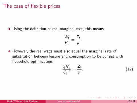
The case of flexible prices

Using the definition of real marginal cost, this means

Wt

Pt=

Zt

µ.

However, the real wage must also equal the marginal rate ofsubstitution between leisure and consumption to be consist withhousehold optimization:

χNηt

C−σt

=Zt

µ. (12)


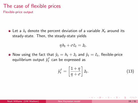
The case of flexible pricesFlexible-price output

Let a xt denote the percent deviation of a variable Xt around itssteady-state. Then, the steady-state yields

ηnt + σct = zt .

Now using the fact that yt = nt + zt and yt = ct , flexible-priceequilibrium output y ft can be expressed as

y ft =

[1 + η

η + σ

]zt . (13)


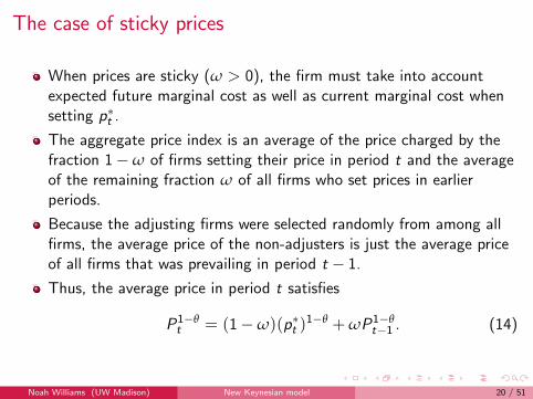
The case of sticky prices

When prices are sticky (ω > 0), the firm must take into accountexpected future marginal cost as well as current marginal cost whensetting p∗t .

The aggregate price index is an average of the price charged by thefraction 1−ω of firms setting their price in period t and the averageof the remaining fraction ω of all firms who set prices in earlierperiods.

Because the adjusting firms were selected randomly from among allfirms, the average price of the non-adjusters is just the average priceof all firms that was prevailing in period t − 1.

Thus, the average price in period t satisfies

P1−θt = (1−ω)(p∗t )

1−θ + ωP1−θt−1 . (14)


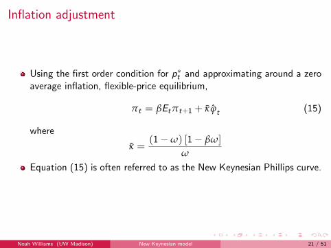
Inflation adjustment

Using the first order condition for p∗t and approximating around a zeroaverage inflation, flexible-price equilibrium,

πt = βEtπt+1 + κ ϕt (15)

where

κ =(1−ω) [1− βω]

ω

Equation (15) is often referred to as the New Keynesian Phillips curve.


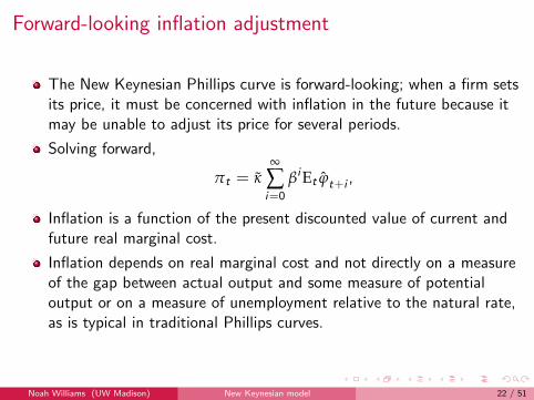
Forward-looking inflation adjustment

The New Keynesian Phillips curve is forward-looking; when a firm setsits price, it must be concerned with inflation in the future because itmay be unable to adjust its price for several periods.

Solving forward,

πt = κ∞

∑i=0

βiEt ϕt+i ,

Inflation is a function of the present discounted value of current andfuture real marginal cost.

Inflation depends on real marginal cost and not directly on a measureof the gap between actual output and some measure of potentialoutput or on a measure of unemployment relative to the natural rate,as is typical in traditional Phillips curves.


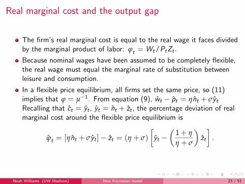
Real marginal cost and the output gap

The firm’s real marginal cost is equal to the real wage it faces dividedby the marginal product of labor: ϕt = Wt/PtZt .

Because nominal wages have been assumed to be completely flexible,the real wage must equal the marginal rate of substitution betweenleisure and consumption.

In a flexible price equilibrium, all firms set the same price, so (11)implies that ϕ = µ−1. From equation (9), wt − pt = ηnt + σytRecalling that ct = yt , yt = nt + zt , the percentage deviation of realmarginal cost around the flexible price equilibrium is

ϕt = [ηnt + σyt ]− zt = (η + σ)

[yt −

(1 + η

η + σ

)zt

].


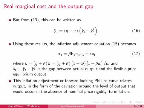
Real marginal cost and the output gap

But from (13), this can be written as

ϕt = (η + σ)(yt − y ft

). (16)

Using these results, the inflation adjustment equation (15) becomes

πt = βEtπt+1 + κxt (17)

where κ = (η + σ) κ = (η + σ) (1−ω) [1− βω] /ω andxt ≡ yt − y ft is the gap between actual output and the flexible-priceequilibrium output.

This inflation adjustment or forward-looking Phillips curve relatesoutput, in the form of the deviation around the level of output thatwould occur in the absence of nominal price rigidity, to inflation.


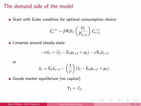
The demand side of the model

Start with Euler condition for optimal consumption choice

C−σt = βRtEt

(Pt

Pt+1

)C−σt+1

Linearize around steady-state:

−σct = (ıt − Etpt+1 + pt)− σEt ct+1

or

ct = Et ct+1 −(

1

σ

)(ıt − Etpt+1 + pt) .

Goods market equilibrium (no capital)

Yt = Ct .


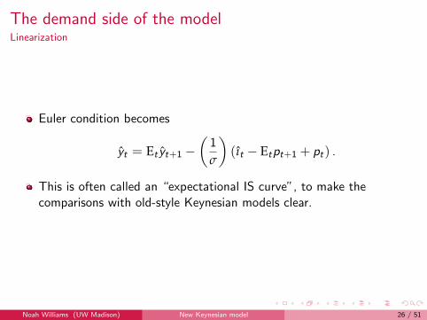
The demand side of the modelLinearization

Euler condition becomes

yt = Et yt+1 −(

1

σ

)(ıt − Etpt+1 + pt) .

This is often called an “expectational IS curve”, to make thecomparisons with old-style Keynesian models clear.


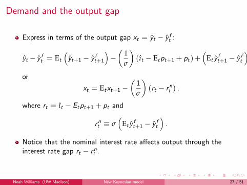
Demand and the output gap

Express in terms of the output gap xt = yt − y ft :

yt − y ft = Et

(yt+1 − y ft+1

)−(

1

σ

)(ıt − Etpt+1 + pt)+

(Et y

ft+1 − y ft

),

or

xt = Etxt+1 −(

1

σ

)(rt − rnt ) ,

where rt = ıt − Etpt+1 + pt and

rnt ≡ σ(

Et yft+1 − y ft

).

Notice that the nominal interest rate affects output through theinterest rate gap rt − rnt .


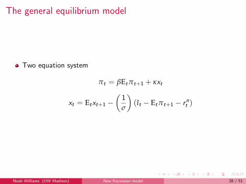
The general equilibrium model

Two equation system

πt = βEtπt+1 + κxt

xt = Etxt+1 −(

1

σ

)(ıt − Etπt+1 − rnt )


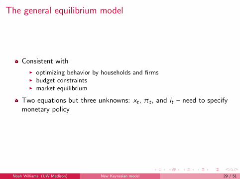
The general equilibrium model

Consistent with

I optimizing behavior by households and firmsI budget constraintsI market equilibrium

Two equations but three unknowns: xt , πt , and it – need to specifymonetary policy


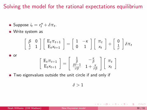
Solving the model for the rational expectations equilibrium

Suppose it = rnt + δπt .

Write system as[β 01σ 1

] [Etπt+1

Etxt+1

]=

[1 −κ0 1

] [πt

xt

]+

[01σ

]δπt

or [Etπt+1

Etxt+1

]=

[1β − κ

ββδ−1

σβ 1 + κσβ

] [πt

xt

]Two eigenvalues outside the unit circle if and only if

δ > 1


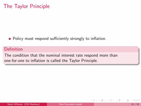
The Taylor Principle

Policy must respond sufficiently strongly to inflation.

Definition

The condition that the nominal interest rate respond more thanone-for-one to inflation is called the Taylor Principle.


Lessons

Policy based on responding to exogenous disturbances does notensure a unique equilibrium.

Policy must respond to endogenous variables.

In particular, the Taylor Principle needs to be satisfied.


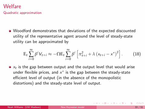
WelfareQuadratic approximation

Woodford demonstrates that deviations of the expected discountedutility of the representative agent around the level of steady-stateutility can be approximated by

Et

∞

∑i=0

βiVt+i ≈ −ΩEt

∞

∑i=0

βi[π2t+i + λ (xt+i − x∗)2

]. (18)

xt is the gap between output and the output level that would ariseunder flexible prices, and x∗ is the gap between the steady-stateefficient level of output (in the absence of the monopolisticdistortions) and the steady-state level of output.


Comparison to a standard loss function

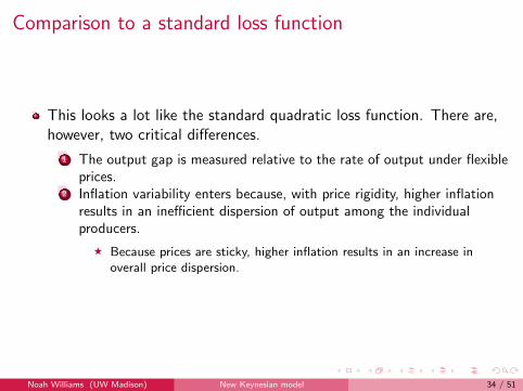
This looks a lot like the standard quadratic loss function. There are,however, two critical differences.

1 The output gap is measured relative to the rate of output under flexibleprices.

2 Inflation variability enters because, with price rigidity, higher inflationresults in an inefficient dispersion of output among the individualproducers.

F Because prices are sticky, higher inflation results in an increase inoverall price dispersion.


Policy weights

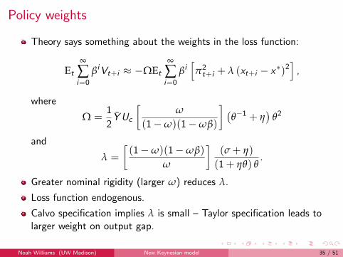
Theory says something about the weights in the loss function:

Et

∞

∑i=0

βiVt+i ≈ −ΩEt

∞

∑i=0


],

where

Ω =1

2Y Uc

[ω

(1−ω)(1−ωβ)

] (θ−1 + η

)θ2

and

λ =

[(1−ω)(1−ωβ)

ω

](σ + η)

(1 + ηθ) θ.

Greater nominal rigidity (larger ω) reduces λ.

Loss function endogenous.

Calvo specification implies λ is small – Taylor specification leads tolarger weight on output gap.


Policy Implication of forward-looking models

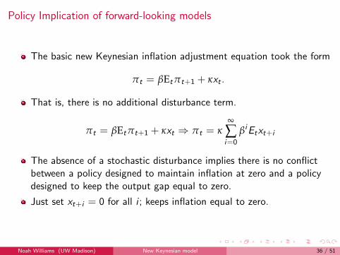
The basic new Keynesian inflation adjustment equation took the form

πt = βEtπt+1 + κxt .

That is, there is no additional disturbance term.

πt = βEtπt+1 + κxt ⇒ πt = κ∞

∑i=0

βiEtxt+i

The absence of a stochastic disturbance implies there is no conflictbetween a policy designed to maintain inflation at zero and a policydesigned to keep the output gap equal to zero.

Just set xt+i = 0 for all i ; keeps inflation equal to zero.


Optimal policy in forward-looking models

Thus, the key implication of the basic new Keynesian model is thatprice stability is the appropriate objective of monetary policy.

No policy conflicts.

When prices are sticky but wages are flexible, the nominal wage canadjust to ensure labor market equilibrium is maintained in the face ofproductivity shocks. Optimal policy should then aim to keep the pricelevel stable.


Policy implications of price stickiness

Models that combine optimizing agents and sticky prices have verystrong policy implications.

When the price level fluctuates, and not all firms are able to adjust,price dispersion results. This causes the relative prices of the differentgoods to vary. If the price level rises, for example, two things happen.

1 The relative price of firms who have not set their prices for a whilefalls. They experience in increase in demand and raise output, whilefirms who have just reset their prices reduce output. This productiondispersion is inefficient.

2 Consumers increase their consumption of the goods whose relativeprice has fallen and reduce consumption of those goods whose relativeprice has risen. This dispersion in consumption reduces welfare.


Cost shocks

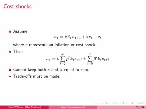
Assumeπt = βEtπt+1 + κxt + et

where e represents an inflation or cost shock.

Then

πt = κ∞

∑i=0

βiEtxt+i +∞

∑i=0

βiEtet+i

Cannot keep both x and π equal to zero.

Trade-offs must be made.


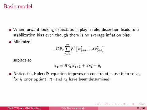
Basic model

When forward-looking expectations play a role, discretion leads to astabilization bias even though there is no average inflation bias.

Minimize

−ΩEt

∞

∑i=0

βi[π2t+i + λx2t+i

]subject to

πt = βEtπt+1 + κxt + et .

Notice the Euler/IS equation imposes no constraint – use it to solvefor it once optimal πt and xt have been determined.


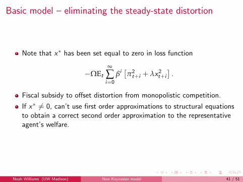
Basic model – eliminating the steady-state distortion

Note that x∗ has been set equal to zero in loss function

−ΩEt

∞

∑i=0

βi[π2t+i + λx2t+i

].

Fiscal subsidy to offset distortion from monopolistic competition.

If x∗ 6= 0, can’t use first order approximations to structural equationsto obtain a correct second order approximation to the representativeagent’s welfare.


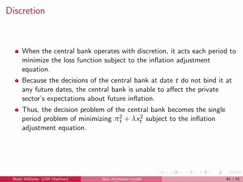
Discretion

When the central bank operates with discretion, it acts each period tominimize the loss function subject to the inflation adjustmentequation.

Because the decisions of the central bank at date t do not bind it atany future dates, the central bank is unable to affect the privatesector’s expectations about future inflation.

Thus, the decision problem of the central bank becomes the singleperiod problem of minimizing π2

t + λx2t subject to the inflationadjustment equation.


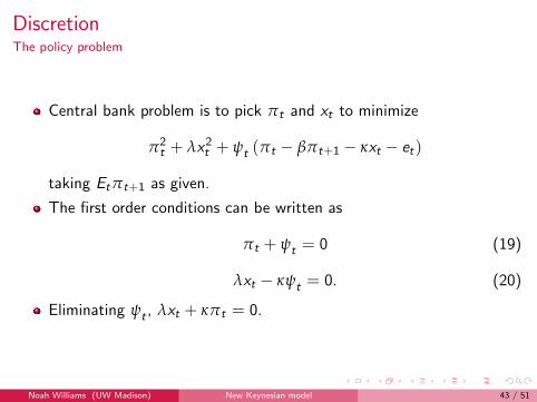
DiscretionThe policy problem

Central bank problem is to pick πt and xt to minimize

π2t + λx2t + ψt (πt − βπt+1 − κxt − et)

taking Etπt+1 as given.

The first order conditions can be written as

πt + ψt = 0 (19)

λxt − κψt = 0. (20)

Eliminating ψt , λxt + κπt = 0.


DiscretionEquilibrium

xt and πt satisfyλxt + κπt = 0.


Then

πt = βEtπt+1 −κ2

λπt + et ⇒ πt =

λβEtπt+1 + λetλ + κ2

.


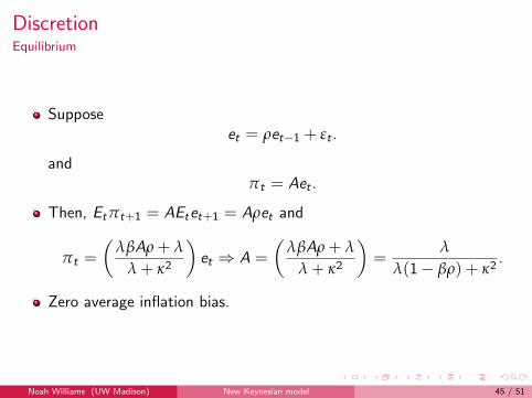
DiscretionEquilibrium

Supposeet = ρet−1 + εt .

andπt = Aet .

Then, Etπt+1 = AEtet+1 = Aρet and

πt =

(λβAρ + λ

λ + κ2

)et ⇒ A =

(λβAρ + λ

λ + κ2

)=

λ

λ(1− βρ) + κ2.

Zero average inflation bias.


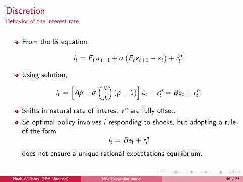
DiscretionBehavior of the interest rate

From the IS equation,

it = Etπt+1 + σ (Etxt+1 − xt) + rnt .

Using solution,

it =[Aρ− σ

( κ

λ

)(ρ− 1)

]et + rnt = Bet + rnt .

Shifts in natural rate of interest rn are fully offset.

So optimal policy involves i responding to shocks, but adopting a ruleof the form

it = Bet + rnt

does not ensure a unique rational expectations equilibrium.


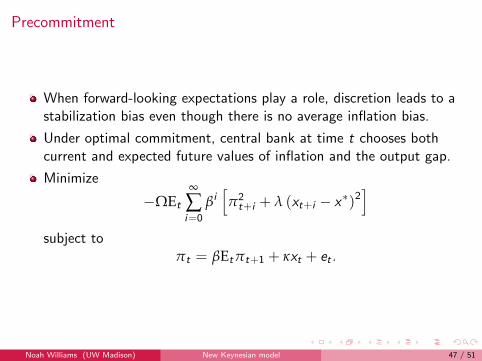
Precommitment

When forward-looking expectations play a role, discretion leads to astabilization bias even though there is no average inflation bias.

Under optimal commitment, central bank at time t chooses bothcurrent and expected future values of inflation and the output gap.

Minimize

−ΩEt

∞

∑i=0


]subject to



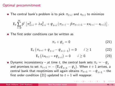
Optimal precommitment

The central bank’s problem is to pick πt+i and xt+i to minimize

Et

∞

∑i=0

βi[π2t+i + λx2t+i + ψt+i (πt+i − βπt+i+1 − κxt+i − et+i )

].

The first order conditions can be written as

πt + ψt = 0 (21)

Et

(πt+i + ψt+i − ψt+i−1

)= 0 i ≥ 1 (22)

Et

(λxt+i − κψt+i

)= 0 i ≥ 0. (23)

Dynamic inconsistency – at time t, the central bank sets πt = −ψt

and promises to set πt+1 = −(Etψt+1 − ψt

). When t + 1 arrives, a

central bank that reoptimizes will again obtains πt+1 = −ψt+1 – thefirst order condition (21) updated to t + 1 will reappear.


Timeless precommitment

An alternative definition of an optimal precommitment policy requiresthe central bank to implement conditions (22) and (23) for allperiods, including the current period so that

πt+i + ψt+i − ψt+i−1 = 0 i ≥ 0

λxt+i − κψt+i = 0 i ≥ 0.

Woodford (1999) has labeled this the “timeless perspective” approachto precommitment.


Timeless precommitment

Under the timeless perspective optimal commitment policy, inflationand the output gap satisfy

πt+i = −(

λ

κ

)(xt+i − xt+i−1) (24)

for all i ≥ 0.

Woodford (1999) has stressed that, even if ρ = 0, so that there is nonatural source of persistence in the model itself, a > 0 and theprecommitment policy introduces inertia into the output gap andinflation processes.

This commitment to inertia implies that the central bank’s actions atdate t allow it to influence expected future inflation. Doing so leadsto a better trade-off between gap and inflation variability than wouldarise if policy did not react to the lagged gap.


Improved trade-off under commitment

The difference in the stabilization response under commitment anddiscretion is the stabilization bias due to discretion.

Consider a positive inflation shock, e > 0.

A given change in current inflation can be achieved with a smaller fallin x if expected future inflation can be reduced:

πt = βEtπt+1 + κxt + et

Requires a commitment to future deflation.

By keeping output below potential (a negative output gap) for severalperiods into the future after a positive cost shock, the central bank isable to lower expectations of future inflation. A fall in Etπt+1 at thetime of the positive inflation shock improves the trade-off betweeninflation and output gap stabilization faced by the central bank.


Documents

The New Keynesian Model - SSCC - Home