The New Keynesian Model: Main Functions

The New Keynesian Model: Main Functions

Vivaldo M. Mendes

ISCTE � Lisbon University Institute

November 2018

(Vivaldo M. Mendes) The New Keynesian Model: Main Functions November 2018 1 / 34

I �What�s is the New Keynesian Model?


What is the New Keynesian Model?

The Old and the New Keynesian Models

1 The new model is the old Keynesian model2 With the usual nominal and/or real rigidities in price setting

Prices are sticky (the baseline version)Nominal wages are rigid downwardsStaggered contractsCapacity utilization constraints

3 Without the problems that pushed the model to serious trouble inthe early 70s

1 "forward looking/rational expectations" instead of "adaptiveexpectations"

2 built upon sound microeconomic foundations3 no permanent trade-o¤ between in�ation and unemployment4 no room for stag�ation

4 A new message: rules instead of discretion by Central Banks in themanagement of monetary policy



Four basic predictions

1 The same usual functions (IS, LM, Aggregate Supply) ...2 Quantitative simulations: crucial element like in the Real BusinessCycle literature

3 Contrary to RBC, there is a key role to monetary policy and a minorrole for �scal policy

4 Four basic predictions (the old model up-side-down):1 the instrument of monetary policy ought to be the short term interestrate,

2 policy should be focused on the control of in�ation,3 in�ation can be reduced by aggressively increasing short term interestrates (see next �gure).

4 the central bank should conduct monetary policy adopting a strategy ofcommitment in a forward-looking environment, instead of discretion.



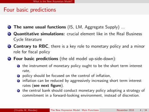
Active interest rate policy by the Fed

The FED now reacts much more aggressively to in�ation than in the "oldtimes"



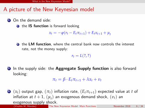
A picture of the New Keynesian model

1 On the demand side:1 the IS function is forward looking

xt = �ϕ(rt � Etπt+1) + Etxt+1 + µt

2 the LM function, where the central bank now controls the interestrate, not the money supply:

rt = L(?, ?)

2 In the supply side: the Aggregate Supply function is also forwardlooking:

πt = β � Etπt+1 + λxt + υt

3 (xt) output gap, (πt) in�ation rate, (Etπt+1) expected value at t ofin�ation at t+ 1, (µt) an exogenous demand shock, (υt) anexogenous supply shock.(Vivaldo M. Mendes) The New Keynesian Model: Main Functions November 2018 6 / 34

The New IS function

The New IS function


The New IS function

The IS function in three steps

1 You may �nd a very ellaborate way of deriving the IS function2 There is a simple and intuitive way to derive it

1 Firstly, get the Euler equation2 Second, log-linearize the Euler equation3 Third, express the Euler equation in terms of percentage deviationsfrom the steady state


The New IS function

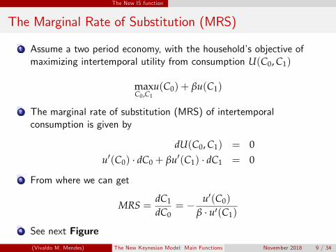
The Marginal Rate of Substitution (MRS)

1 Assume a two period economy, with the household�s objective ofmaximizing intertemporal utility from consumption U(C0, C1)

maxC0,C1

u(C0) + βu(C1)

2 The marginal rate of substitution (MRS) of intertemporalconsumption is given by

dU(C0, C1) = 0u0(C0) � dC0 + βu0(C1) � dC1 = 0

3 From where we can get

MRS =dC1

dC0= � u0(C0)

β � u0(C1)

4 See next Figure(Vivaldo M. Mendes) The New Keynesian Model: Main Functions November 2018 9 / 34

The New IS function

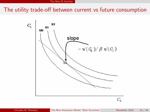
The utility trade-o¤ between current vs future consumption


The New IS function

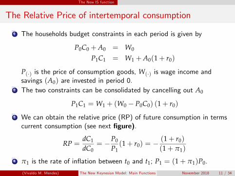
The Relative Price of intertemporal consumption

1 The households budget constraints in each period is given by

P0C0 +A0 = W0

P1C1 = W1 +A0(1+ r0)

P(�) is the price of consumption goods, W(�) is wage income andsavings (A0) are invested in period 0.

2 The two constraints can be consolidated by cancelling out A0

P1C1 = W1 + (W0 � P0C0) (1+ r0)

3 We can obtain the relative price (RP) of future consumption in termscurrent consumption (see next �gure).

RP =dC1

dC0= �P0

P1(1+ r0) = �

(1+ r0)

(1+ π1)

4 π1 is the rate of in�ation between t0 and t1; P1 = (1+ π1)P0.


The New IS function

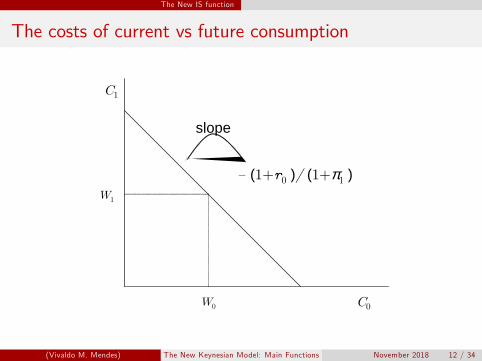
The costs of current vs future consumption

W1

W0

slope

C1

C0

� (1+r0 )/ (1+π1 )


The New IS function

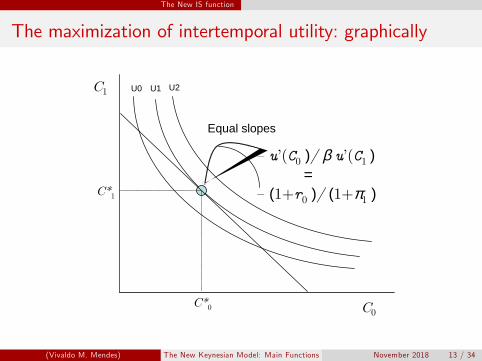
The maximization of intertemporal utility: graphically

� u�(C0 )/ β u�(C1 )

Equal slopes

C1

C0

U0 U1 U2

=� (1+r0 )/ (1+π1 )C*1

C*0


The New IS function

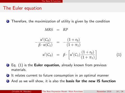
The Euler equation

1 Therefore, the maximization of utility is given by the condition

MRS = RP

� u0(C0)

β � u(C1)= � (1+ r0)

(1+ π1)

u0(C0) = β ��

u0(C1)(1+ r0)

(1+ π1)

�(1)

2 Eq. (1) is the Euler equation, already known from previousmaterials.

3 It relates current to future consumption in an optimal manner4 And as we will show, it is also the basis for the new IS function


The New IS function

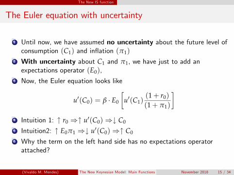
The Euler equation with uncertainty

1 Until now, we have assumed no uncertainty about the future level ofconsumption (C1) and in�ation (π1)

2 With uncertainty about C1 and π1, we have just to add anexpectations operator (E0),

3 Now, the Euler equation looks like

u0(C0) = β � E0

�u0(C1)

(1+ r0)

(1+ π1)

�4 Intuition 1: " r0 )" u0(C0))# C0

5 Intuition2: " E0π1 )# u0(C0))" C0

6 Why the term on the left hand side has no expectations operatorattached?


The New IS function

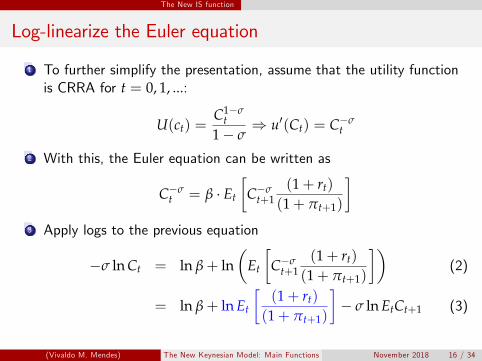
Log-linearize the Euler equation

1 To further simplify the presentation, assume that the utility functionis CRRA for t = 0, 1, ...:

U(ct) =C1�σ

t1� σ

) u0(Ct) = C�σt

2 With this, the Euler equation can be written as

C�σt = β � Et

�C�σ

t+1(1+ rt)

(1+ πt+1)

�3 Apply logs to the previous equation

�σ ln Ct = ln β+ ln�

Et

�C�σ

t+1(1+ rt)

(1+ πt+1)

��(2)

= ln β+ ln Et

�(1+ rt)

(1+ πt+1)

�� σ ln EtCt+1 (3)


The New IS function

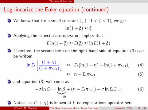
Log-linearize the Euler equation (continued)

1 We know that for a small constant ξ, (�1 < ξ < 1), we get

ln(1+ ξ) � ξ

2 Applying the expectations operator, implies that

E ln(1+ ξ) � E(ξ) � ln E(1+ ξ)

3 Therefore, the second term on the right hand-side of equation (3) canbe written

ln Et

�(1+ rt)

(1+ πt+1)

�� Et [ln(1+ rt)� ln(1+ πt+1)] (4)

� rt � Etπt+1 (5)

4 and equation (3) will come as

�σ ln Ct = ln β|{z}+�0

(rt � Etπt+1)� σ ln EtCt+1 (6)

5 Notice: as (1+ rt) is known at t, no expectations operator here.(Vivaldo M. Mendes) The New Keynesian Model: Main Functions November 2018 17 / 34

The New IS function

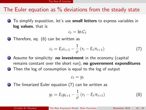
The Euler equation as % deviations from the steady state

1 To simplify exposition, let�s use small letters to express variables inlog values, that is

ct = ln Ct

2 Therefore, eq. (6) can be written as

ct = Etct+1 �1σ(rt � Etπt+1) (7)

3 Assume for simplicity: no investment in the economy (capitalremains constant over the short run), no government expenditures

4 Then the log of consumption is equal to the log of output

ct = yt

5 The linearized Euler equation (7) can be written as

yt = Etyt+1 �1σ(rt � Etπt+1) (8)


The New IS function

The Euler eq. as % deviations from the steady state (II)

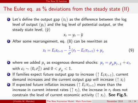
1 Let�s de�ne the output gap (xt) as the di¤erence between the loglevel of output (yt) and the log level of potential output, or thesteady state level, (y)

xt = yt � y2 After some rearrangement, eq. (8) can be rewritten as

xt = Etxt+1 �1σ(rt � Etπt+1) + µt (9)

3 where we added µt as exogenous demand shocks: µt = ρµµt�1 + εt,

with εt � (0, σ2ε) and 0 < ρµ < 1.

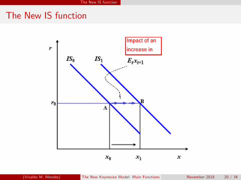
4 If families expect future output gap to increase (" Etxt+1), currentdemand increases and the current output gap will increase (" xt)

5 If expected future in�ation increases (" Etπt+1) more than theincrease in current interest rates (" rt), the increase in rt does notconstrain the level of current economic activity (" xt). See Fig.5.(Vivaldo M. Mendes) The New Keynesian Model: Main Functions November 2018 19 / 34

The New IS function

The New IS function


The New IS function

The New AS function (or theNew Keynesian Phillips Curve)


The New IS function

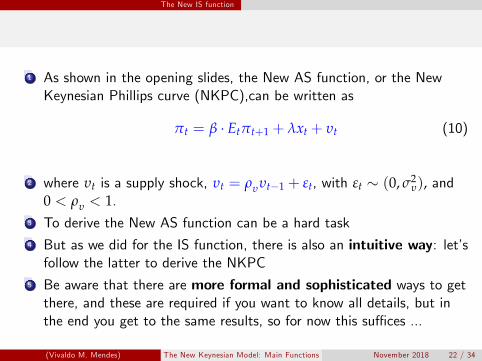
1 As shown in the opening slides, the New AS function, or the NewKeynesian Phillips curve (NKPC),can be written as

πt = β � Etπt+1 + λxt + υt (10)

2 where υt is a supply shock, υt = ρυυt�1 + εt, with εt � (0, σ2υ), and

0 < ρυ < 1.3 To derive the New AS function can be a hard task4 But as we did for the IS function, there is also an intuitive way: let�sfollow the latter to derive the NKPC

5 Be aware that there are more formal and sophisticated ways to getthere, and these are required if you want to know all details, but inthe end you get to the same results, so for now this su¢ ces ...


The New IS function

Assumptions of the New AS function

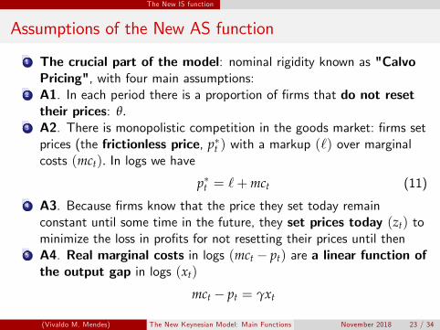
1 The crucial part of the model: nominal rigidity known as "CalvoPricing", with four main assumptions:

2 A1. In each period there is a proportion of �rms that do not resettheir prices: θ.

3 A2. There is monopolistic competition in the goods market: �rms setprices (the frictionless price, p�t ) with a markup (`) over marginalcosts (mct). In logs we have

p�t = `+mct (11)

4 A3. Because �rms know that the price they set today remainconstant until some time in the future, they set prices today (zt) tominimize the loss in pro�ts for not resetting their prices until then

5 A4. Real marginal costs in logs (mct � pt) are a linear function ofthe output gap in logs (xt)

mct � pt = γxt


The New IS function Minimizing the Loss function

Minimizing the Loss function

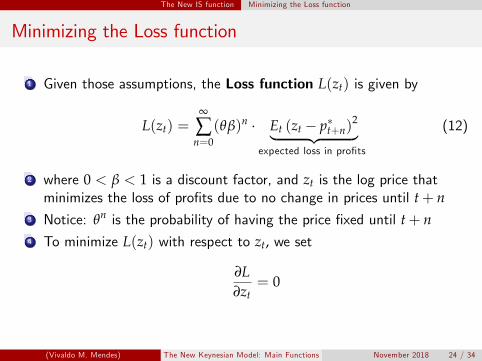
1 Given those assumptions, the Loss function L(zt) is given by

L(zt) =∞

∑n=0(θβ)n � Et (zt � p�t+n)

2| {z }expected loss in pro�ts

(12)

2 where 0 < β < 1 is a discount factor, and zt is the log price thatminimizes the loss of pro�ts due to no change in prices until t+ n

3 Notice: θn is the probability of having the price �xed until t+ n4 To minimize L(zt) with respect to zt, we set

∂L∂zt

= 0



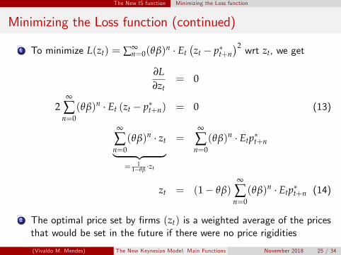
Minimizing the Loss function (continued)

1 To minimize L(zt) = ∑∞n=0(θβ)n � Et

�zt � p�t+n

�2 wrt zt, we get

∂L∂zt

= 0

2∞

∑n=0(θβ)n � Et (zt � p�t+n) = 0 (13)

∞

∑n=0(θβ)n � zt| {z }= 1

1�θβ �zt

=∞

∑n=0(θβ)n � Etp�t+n

zt = (1� θβ)∞

∑n=0(θβ)n � Etp�t+n (14)

2 The optimal price set by �rms (zt) is a weighted average of the pricesthat would be set in the future if there were no price rigidities




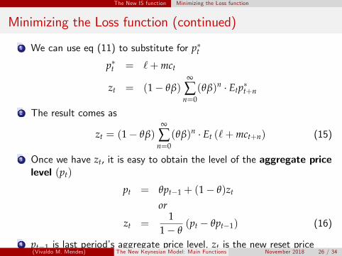
1 We can use eq (11) to substitute for p�tp�t = `+mct

zt = (1� θβ)∞

∑n=0(θβ)n � Etp�t+n

2 The result comes as

zt = (1� θβ)∞

∑n=0(θβ)n � Et (`+mct+n) (15)

3 Once we have zt, it is easy to obtain the level of the aggregate pricelevel (pt)

pt = θpt�1 + (1� θ)zt

or

zt =1

1� θ(pt � θpt�1) (16)

4 pt�1 is last period�s aggregate price level, zt is the new reset price(Vivaldo M. Mendes) The New Keynesian Model: Main Functions November 2018 26 / 34



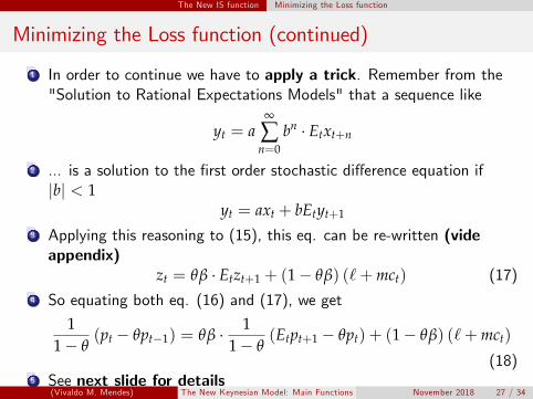
1 In order to continue we have to apply a trick. Remember from the"Solution to Rational Expectations Models" that a sequence like

yt = a∞

∑n=0

bn � Etxt+n

2 ... is a solution to the �rst order stochastic di¤erence equation ifjbj < 1

yt = axt + bEtyt+1

3 Applying this reasoning to (15), this eq. can be re-written (videappendix)

zt = θβ � Etzt+1 + (1� θβ) (`+mct) (17)4 So equating both eq. (16) and (17), we get

11� θ

(pt � θpt�1) = θβ � 11� θ

(Etpt+1 � θpt) + (1� θβ) (`+mct)

(18)5 See next slide for details




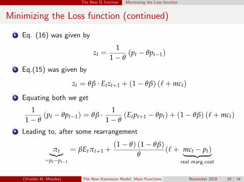
1 Eq. (16) was given by

zt =1

1� θ(pt � θpt�1)

2 Eq.(15) was given by

zt = θβ � Etzt+1 + (1� θβ) (`+mct)

3 Equating both we get

11� θ

(pt � θpt�1) = θβ � 11� θ

(Etpt+1 � θpt) + (1� θβ) (`+mct)

4 Leading to, after some rearrangement

πt|{z}=pt�pt�1

= βEtπt+1 +(1� θ) (1� θβ)

θ(`+ mct � pt)| {z }

real marg.cost




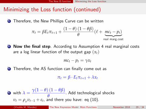
1 Therefore, the New Phillips Curve can be written

πt = βEtπt+1 +(1� θ) (1� θβ)

θ(`+ mct � pt)| {z }

real marg.cost

2 Now the �nal step. According to Assumption 4 real marginal costsare a log linear function of the output gap (xt)

mct � pt = γxt

3 Therefore, the AS function can �nally come out as

πt = β � Etπt+1 + λxt

4 with λ =γ(1� θ) (1� θβ)

θ. Add technological shocks

υt = ρυυt�1 + εt, and there you have: eq (10).



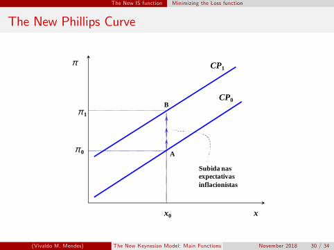
The New Phillips Curve

π

x

CP1

x0

π 0

B

A

CP0

π 1

Subida nasexpectativasinflacionistas



The Central Bank behavior



The Central Bank behavior

1 Until now, we have 3 endogenous variables fxt+s, πt+s, rt+sgs=∞s=0 , but

only two equations (IS, AS or the New Phillips curve).2 So we need another equation in order to have the model determined.3 There are two major ways to close the model:

1 The central bank controls the money supply, and the marketdetermines rt, (the old view)

2 The central bank controls the rt, and the market determines the levelof money in the market (the new view).

4 Next: what is better, the old view or the new view.



Appendix



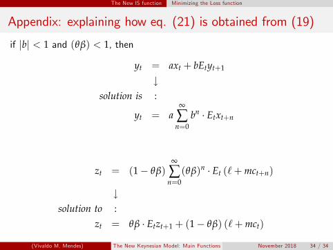
Appendix: explaining how eq. (21) is obtained from (19)

if jbj < 1 and (θβ) < 1, then

yt = axt + bEtyt+1

#solution is :

yt = a∞

∑n=0

bn � Etxt+n

zt = (1� θβ)∞

∑n=0(θβ)n � Et (`+mct+n)

#solution to :

zt = θβ � Etzt+1 + (1� θβ) (`+mct)


Documents

The New Keynesian Model: Main Functions