Embed Size (px)
Citation preview

C E N T R ED ’ É T U D E S P R O S P E C T I V E SE T D ’ I N F O R M A T I O N SI N T E R N A T I O N A L E S
No 2013 � 01
January
DO
CU
ME
NT
DE
TR
AV
AI
L
The Solow Growth Model
with Keynesian Involuntary Unemployment
Riccardo Magnani
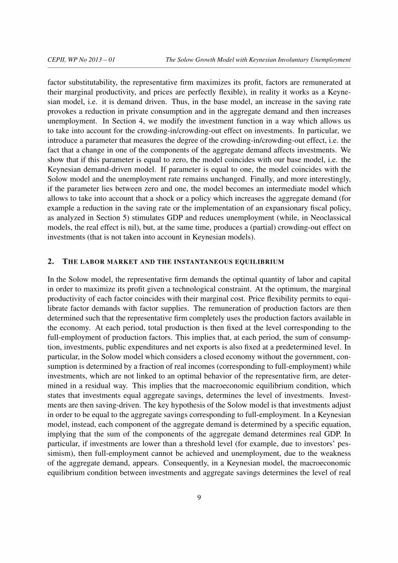
CEPII, WP No 2013 – 01 The Solow Growth Model with Keynesian Involuntary Unemployment
TABLE OF CONTENTS
Non-technical summary . . . . . . . . . . . . . . . . . . . . . . . . . . . 3Abstract . . . . . . . . . . . . . . . . . . . . . . . . . . . . . . . . . 4Résumé non technique . . . . . . . . . . . . . . . . . . . . . . . . . . . 5Résumé court . . . . . . . . . . . . . . . . . . . . . . . . . . . . . . . 61. Introduction and motivation . . . . . . . . . . . . . . . . . . . . . . . . 72. The labor market and the instantaneous equilibrium . . . . . . . . . . . . . . 9
2.1. Under-unemployment equilibrium and factor prices . . . . . . . . . . . . 122.2. The Walras Law. . . . . . . . . . . . . . . . . . . . . . . . . . . 14
3. The Solow model with endogenous unemployment . . . . . . . . . . . . . . 153.1. Instantaneous equilibrium . . . . . . . . . . . . . . . . . . . . . . . 163.2. The steady state and the transition phase towards the long-run equilibrium . . . 183.3. The effect of a change in the saving rate . . . . . . . . . . . . . . . . . 19
4. Introduction of a crowding-in/crowding-out effect on investments . . . . . . . . . 194.1. Instantaneous equilibrium . . . . . . . . . . . . . . . . . . . . . . . 204.2. The steady state . . . . . . . . . . . . . . . . . . . . . . . . . . . 21
5. Introduction of public expenditures . . . . . . . . . . . . . . . . . . . . . 225.1. Instantaneous equilibrium . . . . . . . . . . . . . . . . . . . . . . . 235.2. The steady state . . . . . . . . . . . . . . . . . . . . . . . . . . . 23
6. Introduction of public expenditures with (partial) crowding-out effect on investments . 246.1. Instantaneous equilibrium . . . . . . . . . . . . . . . . . . . . . . . 256.2. The steady state . . . . . . . . . . . . . . . . . . . . . . . . . . . 26
7. Numerical simulations . . . . . . . . . . . . . . . . . . . . . . . . . . 277.1. Transition of an under-capitalized economy . . . . . . . . . . . . . . . . 277.2. Increase in the saving rate . . . . . . . . . . . . . . . . . . . . . . . 277.3. Introduction of public expenditures . . . . . . . . . . . . . . . . . . . 29
8. Conclusions . . . . . . . . . . . . . . . . . . . . . . . . . . . . . . 30References . . . . . . . . . . . . . . . . . . . . . . . . . . . . . . . . 31Appendix . . . . . . . . . . . . . . . . . . . . . . . . . . . . . . . . 32List of working papers released by CEPII . . . . . . . . . . . . . . . . . . . . 34
2
CEPII, WP No 2013 – 01 The Solow Growth Model with Keynesian Involuntary Unemployment
THE SOLOW GROWTH MODELWITH KEYNESIAN INVOLUNTARY UNEMPLOYMENT
Riccardo Magnani
NON-TECHNICAL SUMMARY
Unemployment, which is undoubtedly a fundamental macroeconomic issue, is treated as a short termphenomenon affecting fluctuations, but, surprisingly, is completely neglected in Neoclassical growthmodels. It is also surprising that a fiscal policy or, more generally, a shock which affects one of thecomponents of the aggregate demand, produces completely different effects on GDP and employmentusing Neoclassical supply-driven models or Keynesian demand-driven models. The different visionof the functioning of the economy is translated to the disagreement concerning the implementation ofausterity policies in order to face the current double problem of high public debts and low economicgrowth.
The aim of this paper is to extend the Solow growth model by taking into account for the Keynesianunemployment, i.e. unemployment due to the weakness of aggregate demand. In order to introduce aKeynesian unemployment in the Solow model, we relax the hypothesis that investments are determinedby aggregate savings in order to achieve full-employment. More precisely, the only difference withrespect to the standard Solow model is that we introduce in our model one supplementary equation,the investment function, and one supplementary variable, the unemployment rate. In particular, using avery simple investment function, we show that the instantaneous equilibrium may be characterized bythe presence of involuntary unemployment if investments are below a threshold value. We also showthat, for an under-capitalized economy, the capital per unit of effective labor and the unemployment rateincrease over time during the transition phase, until the economy reaches its steady state which may becharacterized by a positive value of the unemployment rate.
Then, we show that an increase in the saving rate produces a negative effect on unemployment and onGDP, both in the short and in the long run. This result is due to the fact that our base model, even ifit presents many features of Neoclassical models (i.e. the production function allows for factor substi-tutability, the representative firm maximizes its profit, factors are remunerated at their marginal produc-tivity, and prices are perfectly flexible), in reality it works as a Keynesian model, i.e. it is demand driven.Thus, in the base model, an increase in the saving rate provokes a reduction in private consumption andin the aggregate demand and then increases unemployment.
Then, we modify the investment function in a way which allows us to take into account for the crowding-
3

CEPII, WP No 2013 – 01 The Solow Growth Model with Keynesian Involuntary Unemployment
in/crowding-out effect on investments. In particular, we introduce a parameter that measures the degreeof the crowding-in/crowding-out effect, i.e. the fact that a change in one of the components of theaggregate demand affects investments. We show that if this parameter is equal to zero, the model coin-cides with our base model, i.e. the Keynesian demand-driven model. If the parameter is equal to one,the model coincides with the Solow model and the unemployment rate remains unchanged. Finally, andmore interestingly, if the parameter lies between zero and one, the model becomes an intermediate modelwhich allows to take into account that a shock or a policy which increases the aggregate demand (for ex-ample a reduction in the saving rate or the implementation of an expansionary fiscal policy) stimulatesGDP and reduces unemployment (while, in Neoclassical models, the real effect is nil), but, at the sametime, produces a (partial) crowding-out effect on investments (that is not taken into account in Keynesianmodels).
ABSTRACT
The aim of this paper is to extend the Solow model in a way that permits to endogenize unemployment.Starting from a Neoclassical growth model, as the Solow model, we introduce a mechanism that allowsus to determine the Keynesian unemployment, i.e. unemployment that is caused by the weakness of theaggregate demand. Using our base model, that works as a Keynesian demand-driven model, we find thatan increase in the aggregate demand (due to a reduction in the saving rate or to an increase in publicexpenditures) reduces unemployment and stimulates the GDP. Then, we modify the investment functionin order to take into account for the crowding-in/crowding-out effect on investments. This allows usto build a model which is between Neoclassical supply-driven models and Keynesian demand-drivenmodels.
JEL Classification: O40; E13; E12; J60
Keywords: Growth models; Neoclassical models; Keynesian models; Involuntary unemploy-ment.
4

CEPII, WP No 2013 – 01 The Solow Growth Model with Keynesian Involuntary Unemployment
THE SOLOW GROWTH MODELWITH KEYNESIAN INVOLUNTARY UNEMPLOYMENT
Riccardo Magnani
RESUME NON TECHNIQUE
Le chômage, qui est sans nul doute un sujet fondamental en macro-économie, est traité comme un phéno-mène de court terme et, de façon surprenante, est complètement négligé dans les modèles néoclassiquesde croissance. Il est également étonnant de constater que la politique budgétaire ou, plus généralement,un choc affectant l’une des composantes de la demande agrégée produisent des effets complètement dif-férents sur le PIB et l’emploi selon qu’on se situe dans un cadre néoclassique ou keynésien. Cette visiondifférente du fonctionnement de l’économie explique le désaccord qui existe aujourd’hui entre les éco-nomistes quant à l’efficacité à attendre des politiques d’austérité ou de relance pour faire face au doubleproblème posé par les niveaux élevés des dettes publiques et par la faiblesse de la croissance.
Le but de ce papier est de proposer une extension du modèle de croissance de Solow en prenant en comptele chômage keynésien, c’est-à-dire le chômage provoqué par la faiblesse de la demande agrégée. Afind’introduire le chômage keynésien, nous relâchons l’hypothèse du modèle de Solow selon laquelle l’in-vestissement est déterminé par l’épargne agrégée de façon à garantir le plein-emploi. Plus précisément,nous introduisons dans un modèle de Solow standard une équation supplémentaire, la fonction d’inves-tissement, et une variable supplémentaire, le taux de chômage. Avec une fonction d’investissement trèssimple, nous montrons en particulier que l’équilibre instantané de l’économie peut être caractérisé par laprésence de chômage involontaire lorsque les investissements sont en dessous d’une valeur seuil. Nousmontrons aussi que, pour une économie sous-capitalisée, le capital par unité de travail et le taux de chô-mage augmentent au cours de la phase de transition, jusqu’au moment où l’économie atteint son étatd’équilibre qui peut être caractérisé par une valeur positive du taux de chômage.
Nous montrons également que l’augmentation du taux d’épargne produit un effet négatif sur le chômageet le PIB, à la fois à court et à long terme. Ce résultat est dû au fait que notre modèle de base, mêmes’il présente de nombreuses caractéristiques des modèles néoclassiques (la fonction de production est àfacteurs substituables, l’entreprise représentative maximise son profit, les facteurs sont rémunérés à leurproductivité marginale et les prix sont parfaitement flexibles), fonctionne en réalité comme un modèlekeynésien, c’est à dire que la production est déterminée par la demande. Ainsi, une augmentation du tauxd’épargne provoque une réduction de la consommation privée et de la demande agrégée, ce qui affectenégativement le chômage.
5
CEPII, WP No 2013 – 01 The Solow Growth Model with Keynesian Involuntary Unemployment
Nous modifions alors la fonction d’investissement de façon à prendre en considération l’ampleur del’effet d’éviction, c’est à dire la mesure dans laquelle un changement dans l’une des composantes dela demande agrégée affecte les investissements. Pour cela, nous introduisons un paramètre mesurant ledegré d’éviction. Si ce paramètre est égal à zéro, le modèle coïncide avec notre modèle de base, à savoirun modèle keynésien où la production est déterminée par la demande. Si le paramètre est égal à un, lemodèle coïncide avec le modèle de Solow et le taux de chômage reste inchangé. Enfin, si le paramètreest compris entre zéro et un, le modèle devient un modèle intermédiaire qui permet à la fois de prendreen compte le fait qu’un choc ou une stimulation de la demande agrégée (par exemple une réductiondu taux d’épargne ou une politique budgétaire expansionniste) provoquent un effet positif sur le PIBet réduisent le chômage (dans un modèle néoclassique, l’effet réel serait nul), mais qu’ils produisenten même temps un effet d’éviction (partielle) sur les investissements (effet qui n’existerait pas dans unmodèle keynésien).
RESUME COURT
Le but de ce papier est de proposer une extension du modèle de croissance de Solow qui permet d’endogénéiserle chômage. A partir du modèle de Solow, nous introduisons un mécanisme qui nous permet de déter-miner le chômage keynésien, c’est-à-dire le chômage provoqué par la faiblesse de la demande agrégée.Notre modèle de base fonctionne alors comme un modèle keynésien où la production est déterminée parla demande : l’augmentation de la demande agrégée (due à une réduction du taux d’épargne ou à uneaugmentation des dépenses publiques) réduit le chômage et stimule le PIB. Ensuite, nous modifions lafonction d’investissement, afin de tenir compte de l’effet d’éviction sur les investissements. Cela nouspermet de construire un modèle qui se situe entre les modèles néoclassiques où la production est déter-minée par l’offre des facteurs et les modèles keynésiens où la production est déterminée par la demande.
Classification JEL : F40 ; C63 ; C68
Mots clés : Modèles de croissance ; Modèles Néoclassiques ; Modèles Keynésiens ; Chômageinvolontaire.
6
CEPII, WP No 2013 – 01 The Solow Growth Model with Keynesian Involuntary Unemployment
THE SOLOW GROWTH MODELWITH KEYNESIAN INVOLUNTARY UNEMPLOYMENT
Riccardo Magnani∗
1. INTRODUCTION AND MOTIVATION
It is quite surprising that Neoclassical growth models have completely neglected a fundamentalmacroeconomic issue such as unemployment. Unemployment is treated as a short term phe-nomenon affecting fluctuations, but not as a long term issue. In contrast, empirical data (forexample for the US) show that not only GDP growth rates but also unemployment rates fluctu-ate around a trend that would deserve to be taken into account in growth models.
It is also surprising that a macroeconomic shock such a change in public expenditures or, moregenerally, in one of the components of the aggregate demand, produces completely differenteffects whether using a Neoclassical supply-driven model or a Keynesian demand-driven model.In particular, the different vision of the functioning of the economy reflects the disagreementconcerning the implementation of austerity policies in order to face the current double problemof high public debts and low economic growth.
The aim of this paper is to propose a growth model which extends the standard Solow modelby taking into account for the unemployment. Starting from the Solow model, we introducea mechanism that allows us to endogenize the unemployment rate. In particular, the kind ofunemployment considered in our paper is the Keynesian unemployment. For Keynesian unem-ployment we mean the unemployment that is caused by the weakness of the aggregate demand.
In order to introduce a Keynesian unemployment in the Solow model it is necessary to relax thefundamental hypothesis made in the Classical and Neoclassical theory, i.e. the full-utilizationof the production factors. Very few works have considered the possibility of under-utilization ofproduction factors in a Neoclassical framework. Concerning the utilization of capital, Chatter-jee (2005) examines the implications of capital utilization for the dynamics of economic growthand convergence. Starting from the evidence that in the economies there is less than full uti-lization of capital and that the depreciation rate is not constant, he shows that endogenizing therate of capital utilization can lead to empirically plausible speeds of convergence in economicgrowth models. Concerning the utilization of labor, the only paper in the literature that in ourknowledge analyzed a Solow model with endogenous Keynesian unemployment is by Back-house (1981). He presented a model where the long-run equilibrium growth path is the "Solow∗CEPN, Université de Paris 13, and CEPII. E-mail: [email protected]. I am grateful to Benjamin
Carton for his useful comments. The usual disclaimer applies.
7

CEPII, WP No 2013 – 01 The Solow Growth Model with Keynesian Involuntary Unemployment
steady state" and where the short-run equilibrium, described by the IS-LM curves, permits thepresence of unemployment. According to the author, the short-run equilibrium, defined "in theKeynesian manner" by assuming that the nominal wage and the capital stock are constant, ischaracterized by two types of disequilibrium that differentiate the Keynesian model from theNeoclassical model: the presence of unemployment (caused by wage stickiness) and the factthat the rate of interest is different from the marginal product of capital (since the capital stockis fixed in the short run). Then, the author shows that the economy converges towards a steadystate characterized by full-employment.
We do not agree with the view that Keynesian unemployment is caused to wage rigidity. Even ifone of the Keynesian arguments is that flexible money wages produces destabilizing effects inthe economy,1 it is wrong to argue that in the Keynesian view unemployment is caused by wagerigidity. In fact, if unemployment was provoked by wage rigidity, full-employment could beachieved by reducing the wage level. But this is exactly the contrary of the Keynesian view: areduction in the wage level reduces households’ income, contracts consumption, and producesnegative effects on the real activity and employment. Of course, wage rigidity is one of thecauses of unemployment but, in the Keynesian view, the key element explaining unemploymentis the weakness of the aggregate demand and not wage rigidity.
In our paper, we first discuss in Section 2 the characteristics of the labor market and of the in-stantaneous equilibrium in the presence of Keynesian unemployment, i.e. in the case in whichthe weakness of the aggregate demand provokes involuntary unemployment. In particular, wecompare our view of the labor market with the one of Patinkin (1965) and of the disequilib-rium theory (Benassy, 1975, Malinvaud, 1977, and Barro and Grossman, 1971). In Section3, we present our base model which extends the Solow model in order to endogenize the un-employment rate. More precisely, we relaxe the hypothesis that investments are determined byaggregate savings in order to achieve full-employment. Thus, the only difference with respect tothe standard Solow model is that we introduce one supplementary equation, i.e. the investmentfunction, and one supplementary variable, i.e. the unemployment rate. In particular, using avery simple investment function, we show that the instantaneous equilibrium may be character-ized by the presence of involuntary unemployment if investments are below a threshold value.Concerning the dynamics, we show that an under-developed economy converges towards itssteady-state equilibrium that may be characterized by a positive value of the unemploymentrate and, during the transition phase, the capital per unit of effective labor increases and theunemployment rate increases over time, until the economy reaches its steady state. Then, weshow that an increase in the saving rate produces a negative effect on employment and on GDP,both in the short and in the long run. This result is due to the fact that our base model, evenif it presents many features of Neoclassical models (i.e. the production function allows for
1Keynes observed that a policy of flexible money wages "would be to cause a great instability of prices, so violentperhaps as to make business calculations futile in an economic society functioning after the manner of that in whichwe live. To suppose that a flexible wage policy is a right and proper adjunct of a system which on the whole is oneof laissez-faire, is the opposite of the truth" (1936, p. 269).
8
CEPII, WP No 2013 – 01 The Solow Growth Model with Keynesian Involuntary Unemployment
factor substitutability, the representative firm maximizes its profit, factors are remunerated attheir marginal productivity, and prices are perfectly flexible), in reality it works as a Keyne-sian model, i.e. it is demand driven. Thus, in the base model, an increase in the saving rateprovokes a reduction in private consumption and in the aggregate demand and then increasesunemployment. In Section 4, we modify the investment function in a way which allows usto take into account for the crowding-in/crowding-out effect on investments. In particular, weintroduce a parameter that measures the degree of the crowding-in/crowding-out effect, i.e. thefact that a change in one of the components of the aggregate demand affects investments. Weshow that if this parameter is equal to zero, the model coincides with our base model, i.e. theKeynesian demand-driven model. If parameter is equal to one, the model coincides with theSolow model and the unemployment rate remains unchanged. Finally, and more interestingly,if the parameter lies between zero and one, the model becomes an intermediate model whichallows to take into account that a shock or a policy which increases the aggregate demand (forexample a reduction in the saving rate or the implementation of an expansionary fiscal policy,as analyzed in Section 5) stimulates GDP and reduces unemployment (while, in Neoclassicalmodels, the real effect is nil), but, at the same time, produces a (partial) crowding-out effect oninvestments (that is not taken into account in Keynesian models).
2. THE LABOR MARKET AND THE INSTANTANEOUS EQUILIBRIUM
In the Solow model, the representative firm demands the optimal quantity of labor and capitalin order to maximize its profit given a technological constraint. At the optimum, the marginalproductivity of each factor coincides with their marginal cost. Price flexibility permits to equi-librate factor demands with factor supplies. The remuneration of production factors are thendetermined such that the representative firm completely uses the production factors available inthe economy. At each period, total production is then fixed at the level corresponding to thefull-employment of production factors. This implies that, at each period, the sum of consump-tion, investments, public expenditures and net exports is also fixed at a predetermined level. Inparticular, in the Solow model which considers a closed economy without the government, con-sumption is determined by a fraction of real incomes (corresponding to full-employment) whileinvestments, which are not linked to an optimal behavior of the representative firm, are deter-mined in a residual way. This implies that the macroeconomic equilibrium condition, whichstates that investments equal aggregate savings, determines the level of investments. Invest-ments are then saving-driven. The key hypothesis of the Solow model is that investments adjustin order to be equal to the aggregate savings corresponding to full-employment. In a Keynesianmodel, instead, each component of the aggregate demand is determined by a specific equation,implying that the sum of the components of the aggregate demand determines real GDP. Inparticular, if investments are lower than a threshold level (for example, due to investors’ pes-simism), then full-employment cannot be achieved and unemployment, due to the weaknessof the aggregate demand, appears. Consequently, in a Keynesian model, the macroeconomicequilibrium condition between investments and aggregate savings determines the level of real
9
CEPII, WP No 2013 – 01 The Solow Growth Model with Keynesian Involuntary Unemployment
GDP. In other words, the introduction of a macroeconomic investment function, which is notdirectly related to the optimal behavior of the representative firm, implies that the competitiveequilibrium may be characterized by the presence of unemployment.
Consider now the labor market. Patinkin (1965) asserted that the equilibrium real wage rate isthe level that equates the amounts demanded and supplied of labor, i.e. the level that guaran-tees the labor market clearing (1965, p. 203). Given that in the Keynesian theory the presenceof involuntary unemployment implies that the labor market is not cleared, Patinkin states that"Keynesian economics is the economics of unemployment disequilibrium" (1965, pp. 337-338).Patinkin (1965) and Barro and Grossman (1971) analyzed, in this context of general disequilib-rium, the effect of a reduction in aggregate demand.2 This induces a reduction in employmentand, in the case in which the wage rate remains unchanged, the quantity of labor demandedbecomes lower than the full-employment level. However, in their analysis, the quantity of labordemanded does not belong to the marginal productivity of labor curve. In particular, this off-demand-curve analysis defended by Patinkin (1965) and Barro and Grossman (1971) impliesthat, for a given level of employment lower than full-employment, the real wage is lower thanthe marginal productivity of labor, which is completely incoherent with the firm’s profit maxi-mization. It is interesting to note that even Keynes asserted that in a competitive economy thereal wage is equal to the marginal product of labor (1936, pp. 5 and 17).
The Patinkin’s view of Keynesian unemployment has been widely criticized by Davidson (1967and 1983). According to Davidson, the marginal productivity of labor used by Patinkin and, ingeneral, by Neoclassical economists does not represent the labor demand curve in an economybased on Keynes’s theory. In particular, Davidson states that the intersection of the aggregatesupply and demand curves determines the equilibrium level of employment and the marginalproductivity of labor has to be interpreted as a market equilibrium curve which determines, fora given the level of employment, the equilibrium real wage.
Following Davidson (1967 and 1983), once the production level is determined by the aggregatedemand, the level of employment is given by the inverse of the production function, Ld =F−1(Y ), i.e. employment represents the quantity of labor necessary to produce Y . Given thenumber of individuals employed, it is possible to determine the unemployment rate: u = Ls−Ld
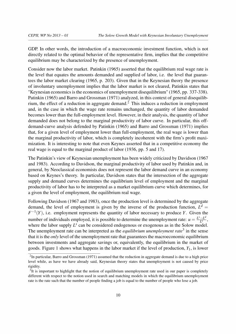
Ls ,where the labor supply Ls can be considered endogenous or exogenous as in the Solow model.The unemployment rate can be interpreted as the equilibrium unemployment rate3 in the sensethat it is the only level of the unemployment rate that guarantees the macroeconomic equilibriumbetween investments and aggregate savings or, equivalently, the equilibrium in the market ofgoods. Figure 1 shows what happens in the labor market if the level of production, Y1, is lower
2In particular, Barro and Grossman (1971) assumed that the reduction in aggregate demand is due to a high pricelevel while, as have we have already said, Keynesian theory states that unemployment is not caused by pricerigidity.
3It is important to highlight that the notion of equilibrium unemployment rate used in our paper is completelydifferent with respect to the notion used in search and matching models in which the equilibrium unemploymentrate is the rate such that the number of people finding a job is equal to the number of people who lose a job.
10
CEPII, WP No 2013 – 01 The Solow Growth Model with Keynesian Involuntary Unemployment
Figure 1 – Involuntary unemployment in thelabor market (first interpretation)
�� ��
�����
��� = �� ��� = �� ∙ 1 − ���
Involuntary unemployment
��
�
�
��
�
Figure 2 – Involuntary unemployment in thelabor market (second interpretation)
�� ��
�����
���
Involuntary unemployment
��
�
�
�
� ∙ 1 − ���
than the full-employment level. The level of employment, LdB, is determined by the inverse of the
production function corresponding to the production level Y1. The real wage rate is determinedalong with the labor demand curve, and the difference between labor supply, supposed to beexogenous and equal to L, and labor demand determines involuntary unemployment.
The mechanisms of the labor market that we have described are essentially equivalent to thatdiscussed by Davidson (1967 and 1983), i.e. the aggregate demand determines the level of pro-duction which in turn determines the level of employment, while the marginal productivity oflabor determines the level of the real wage. However, we think that the fact that the wage rateis determined by the level of the marginal productivity of labor is not completely satisfactory inorder to explain the functioning of the labor market. In fact, the equality between the marginalproductivity of labor and the real wage indicates that, in order to maximize profits, the quantityof labor demanded by the representative firm must be such that the marginal productivity oflabor coincides with the real wage. Thus, this equality cannot determine the real wage. In addi-tion, if the quantity of labor demanded has already been determined (given that the productionlevel is determined by the aggregate demand), then firms have nothing to maximize implyingthat the first order condition for profit maximization is useless.
An alternative way to analyze the labor market, presented in Figure 2, consists to consider thatthe macroeconomic condition determines the equilibrium unemployment rate, uB. Then, it ispossible to plot the (vertical) curve representing the total quantity of labor supplied, L · (1−uB). The profit-maximization condition determines the labor demand function, Ld = f
(wp
),
as in standard Neoclassical models. The intersection between the labor demand curve andthe vertical curve representing the effective quantity of labor supplied determines the quantityof labor employed, Ld
B = L · (1− uB), and the "equilibrium" wage rate(
wp
)B. Finally, the
production function determines the level of production level depending on the quantity of labor
11
CEPII, WP No 2013 – 01 The Solow Growth Model with Keynesian Involuntary Unemployment
employed, Y1 = F(LdB,K).
A very important aspect to note is that point A in both figures, i.e. the intersection between labordemand and labor supply, does not represent an equilibrium in the case in which the aggregatedemand (and then the production level) is equal to Y1, i.e. lower than the full-employment level.In fact, at point A, aggregate saving is greater than investments or, equivalently, production isgreater than aggregate demand. In contrast, point B in both figures represents the equilibriumof the economy in the case in which aggregate demand (and then the production level) is equalto Y1 < Y . This equilibrium can be defined as an under-employment equilibrium, in the sensethat the weakness of the aggregate demand provokes involuntary unemployment. Nevertheless,it is an equilibrium: the market of goods and services is in equilibrium since the production isequal to the aggregate demand, and the labor market is in equilibrium since the demand of laboris equal to the effective quantity of labor supplied.
2.1. Under-unemployment equilibrium and factor prices
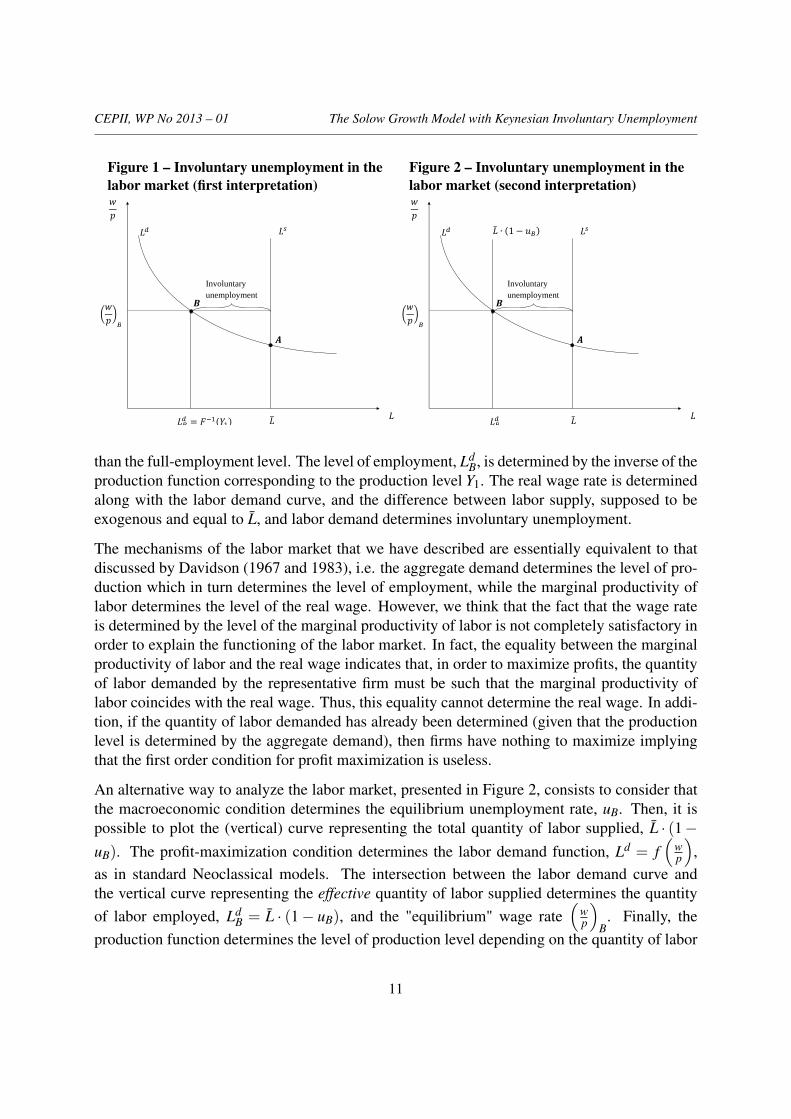
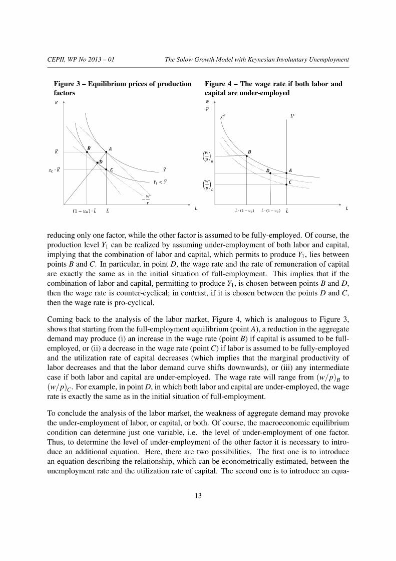
Figures 1 and 2 in the previous section have illustrated that the wage rate is greater in a sit-uation of under-employment equilibrium than in a situation of full-employment equilibrium.In other words, starting from full-employment, a reduction in the aggregate demand provokesinvoluntary unemployment and increases the level of the wage rate. The wage rate is thencounter-cyclical. The same result can be obtained by considering the isoquants of production(see Figure 3). Consider, first, a full-employment situation in which the production level is Yand the disposable capital (K) and labor (L) are completely used. In this case, the equilibriumprices of the production factors are given by the slope of the line tangent to the isoquant at pointA. Then, consider a reduction in the aggregate demand which reduces production (Y1 < Y ) andprovokes involuntary unemployment, with the unemployment rate equal to uB. By supposingthat capital is still full-employed, the equilibrium prices of the production factors are given bythe slope of the line tangent to the new isoquant at point B. The new slope is clearly greater,in absolute value, with respect to the previous one, implying that, with respect to the initialsituation of full-employment, the wage rate is greater and the rate of remuneration of capital islower. This result, which is perfectly analogous to that presented in the previous section, is dueto the fact that capital is supposed to be fully-employed. It is then interesting to analyze theeffect on the equilibrium prices of the production factors in the case in which the hypothesis offull-employment of capital is relaxed.
Suppose that the production level Y1 is realized with full-employment of labor and under-employment of capital. The economy produces Y1 by using L and zC ·K, where z representsthe utilization rate of capital. In this case, the equilibrium prices of the production factors aregiven by the slope of the line tangent to the new isoquant at point C, implying that, with respectto the initial situation of full-employment, the wage rate is lower and the rate of remunerationof capital is greater. In this case, the wage rate is pro-cyclical.
Points B and C represent two extreme cases in which the reduction in production is obtained by
12
CEPII, WP No 2013 – 01 The Solow Growth Model with Keynesian Involuntary Unemployment
Figure 3 – Equilibrium prices of productionfactors
��
�
�
�
��
� ��
�� < ��
1 − �� ∙ ��
� �� ∙ ��
−�
�
�
Figure 4 – The wage rate if both labor andcapital are under-employed
�� ��
�����
� ∙ �1 − ���
��
�
�
�
�
� �����
�
� ∙ �1 − ���
reducing only one factor, while the other factor is assumed to be fully-employed. Of course, theproduction level Y1 can be realized by assuming under-employment of both labor and capital,implying that the combination of labor and capital, which permits to produce Y1, lies betweenpoints B and C. In particular, in point D, the wage rate and the rate of remuneration of capitalare exactly the same as in the initial situation of full-employment. This implies that if thecombination of labor and capital, permitting to produce Y1, is chosen between points B and D,then the wage rate is counter-cyclical; in contrast, if it is chosen between the points D and C,then the wage rate is pro-cyclical.
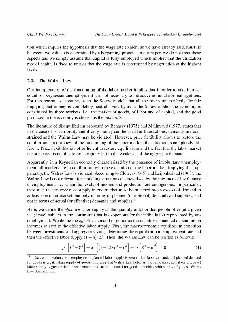
Coming back to the analysis of the labor market, Figure 4, which is analogous to Figure 3,shows that starting from the full-employment equilibrium (point A), a reduction in the aggregatedemand may produce (i) an increase in the wage rate (point B) if capital is assumed to be full-employed, or (ii) a decrease in the wage rate (point C) if labor is assumed to be fully-employedand the utilization rate of capital decreases (which implies that the marginal productivity oflabor decreases and that the labor demand curve shifts downwards), or (iii) any intermediatecase if both labor and capital are under-employed. The wage rate will range from (w/p)B to(w/p)C. For example, in point D, in which both labor and capital are under-employed, the wagerate is exactly the same as in the initial situation of full-employment.
To conclude the analysis of the labor market, the weakness of aggregate demand may provokethe under-employment of labor, or capital, or both. Of course, the macroeconomic equilibriumcondition can determine just one variable, i.e. the level of under-employment of one factor.Thus, to determine the level of under-employment of the other factor it is necessary to intro-duce an additional equation. Here, there are two possibilities. The first one is to introducean equation describing the relationship, which can be econometrically estimated, between theunemployment rate and the utilization rate of capital. The second one is to introduce an equa-
13
CEPII, WP No 2013 – 01 The Solow Growth Model with Keynesian Involuntary Unemployment
tion which implies the hypothesis that the wage rate (which, as we have already said, must liebetween two values) is determined by a bargaining process. In our paper, we do not treat theseaspects and we simply assume that capital is fully-employed which implies that the utilizationrate of capital is fixed to unit or that the wage rate is determined by negotiation at the highestlevel.
2.2. The Walras Law
Our interpretation of the functioning of the labor market implies that in order to take into ac-count for Keynesian unemployment it is not necessary to introduce nominal nor real rigidities.For this reason, we assume, as in the Solow model, that all the prices are perfectly flexibleimplying that money is completely neutral. Finally, as in the Solow model, the economy isconstituted by three markets, i.e. the market of goods, of labor and of capital, and the goodproduced in the economy is chosen as the numéraire.
The literature of disequilibrium proposed by Benassy (1975) and Malinvaud (1977) states thatin the case of price rigidity and if only money can be used for transactions, demands are con-strained and the Walras Law may be violated. However, price flexibility allows to restore theequilibrium. In our view of the functioning of the labor market, the situation is completely dif-ferent. Price flexibility is not sufficient to restore equilibrium and the fact that the labor marketis not cleared is not due to price rigidity but to the weakness of the aggregate demand.
Apparently, in a Keynesian economy characterized by the presence of involuntary unemploy-ment, all markets are in equilibrium with the exception of the labor market, implying that, ap-parently, the Walras Law is violated. According to Clower (1965) and Leijonhufvud (1968), theWalras Law is not relevant for modeling situations characterized by the presence of involuntaryunemployment, i.e. when the levels of income and production are endogenous. In particular,they state that an excess of supply in one market must be matched by an excess of demand inat least one other market, but only in terms of planned (or notional) demands and supplies, andnot in terms of actual (or effective) demands and supplies.4
Here, we define the effective labor supply as the quantity of labor that people offer (at a givenwage rate) subject to the constraint (that is exogenous for the individuals) represented by un-employment. We define the effective demand of goods as the quantity demanded depending onincomes related to the effective labor supply. First, the macroeconomic equilibrium conditionbetween investments and aggregate savings determines the equilibrium unemployment rate andthen the effective labor supply (1−u) ·Ls. Then, the Walras Law can be written as follows:
p ·[Y s−Y d
]+w ·
[(1−u) ·Ls−Ld
]+ r ·
[Ks−Kd
]= 0 (1)
4In fact, with involuntary unemployment, planned labor supply is greater than labor demand, and planned demandfor goods is greater than supply of goods, implying that Walras Law hold. At the same time, actual (or effective)labor supply is greater than labor demand, and actual demand for goods coincides with supply of goods. WalrasLaw does not hold.
14
CEPII, WP No 2013 – 01 The Solow Growth Model with Keynesian Involuntary Unemployment
In particular, by supposing that a fraction 1− s of the real income is consumed and by notingby I investments, the effective demand of goods is given by
Y d = (1− s) ·[
wp· (1−u) ·Ls +
rp·Ks]+ I.
In contrast, the following Walras Law is violated:
p ·[Y s−Y d
]+w ·
[Ls−Ld
]+ r ·
[Ks−Kd
]6= 0 (2)
In fact, if Ls = Ld and Ks =Kd , then (1−s) ·(
wp ·L
s + rp ·K
s)+I represents the notional demand
Y d , that is different from Y s.
Walras Law defined in equation 1 always holds, with equilibrium prices or with disequilibriumprices. One of the three equilibrium conditions, i.e. Y s = Y d , or (1−u) ·Ls = Ld , or Ks = Kd ,is redundant, and the good produced in the economy can be used as numéraire, implying p = 1.An interesting case of disequilibrium prices is the case in which the real wage is fixed at the(disequilibrium) level that permits to achieve the full-employment Ld = Ls. In this case, the realwage is then fixed at a level lower than the equilibrium level. Then, there is an excess demandof labor, i.e. Ld > (1−u) ·Ls, and an excess supply of goods, i.e. Y s > Y d .
3. THE SOLOW MODEL WITH ENDOGENOUS UNEMPLOYMENT
Here we present our base model which extends the Solow model by introducing Keynesian un-employment and by supposing that capital is fully-employed. From one hand, our model is aNeoclassical model in the sense that the production function allows for factor substitutability,the representative firm maximizes its profit, factors are remunerated at their marginal produc-tivity, and all prices are perfectly flexible.5 On the other hand, the model works as a Keynesianmodel. Even if the money market is not taken into account, our model is demand-driven and, inparticular, if the level of aggregate demand is low, unemployment appears.
As in the Solow model, the production function is a Cobb-Douglas function with labor-augmentingproductivity:
Y (t) = K(t)α · [A(t) ·L(t) · (1−u(t))]1−α (3)
where K(t) represents the capital stock, A(t) represents the productivity level assumed to growat a constant rate gA, L(t) represents the working-age population assumed to grow at a constant
5Given that prices are assumed to be perfectly flexible, money is completely neutral. It is then useless to introducein our model the Keynesian LM curve M
p = Md
p (r,Y ). This equation would determine the price level implying thata change in money supply M provokes a proportional change in p, no change in relative prices and then no realeffects.
15
CEPII, WP No 2013 – 01 The Solow Growth Model with Keynesian Involuntary Unemployment
rate n, and u(t) represents the unemployment rate. L(t) · (1− u(t)) represents the number ofworkers6 and A(t) ·L(t) · (1− u) represents the number of units of effective labor. The initiallevel of productivity and of the working-age population are normalized to 1, then: A(t) = egAt
and L(t) = ent . Finally, we define A(t) ·L(t) as the number of units of effective potential labor,in the sense that it represents the number of units of effective labor in the case full-employment,u(t) = 0.
Before presenting the resolution of the model, it is important to detail the notation used:
• The capital per unit of effective potential labor is defined as:
k(t) =K(t)
A(t) ·L(t)
• The capital per unit of effective labor is defined as:
k(t) =K(t)
A(t) ·L(t) · (1−u(t))=
k(t)1−u(t)
• Real GDP is then given by:
Y (t) =
[K(t)
A(t) ·L(t) · (1−u(t))
]α
·A(t) ·L(t) · (1−u(t)) = k(t)α ·A(t) ·L(t) · (1−u(t))
=
[K(t)
A(t) ·L(t)
]α
·A(t) ·L(t) · (1−u(t))1−α = k(t)α ·A(t) ·L(t) · (1−u(t))1−α
• Real GDP per unit of effective potential labor is given by:
y(t) =Y (t)
A(t) ·L(t)= k(t)α · (1−u(t))1−α
3.1. Instantaneous equilibrium
The macroeconomic equilibrium condition states that investments are equal to aggregate sav-ings. In a closed economy without government and by assuming that the representative agentsaves a constant fraction s of his revenue Y , the macroeconomic equilibrium condition is:
I(t) = s ·Y (t)
The key assumption of our model is that investments are not determined by the macroeco-nomic equilibrium condition, i.e. investments are not saving-driven, but they are determined
6Note that even in standard Neoclassical models L(t) · (1− u(t)) represents the number of workers. The onlydifference is that in standard Neoclassical models (1−u(t)) is exogenous and constant and then it does not appearin the analytical resolution.
16
CEPII, WP No 2013 – 01 The Solow Growth Model with Keynesian Involuntary Unemployment
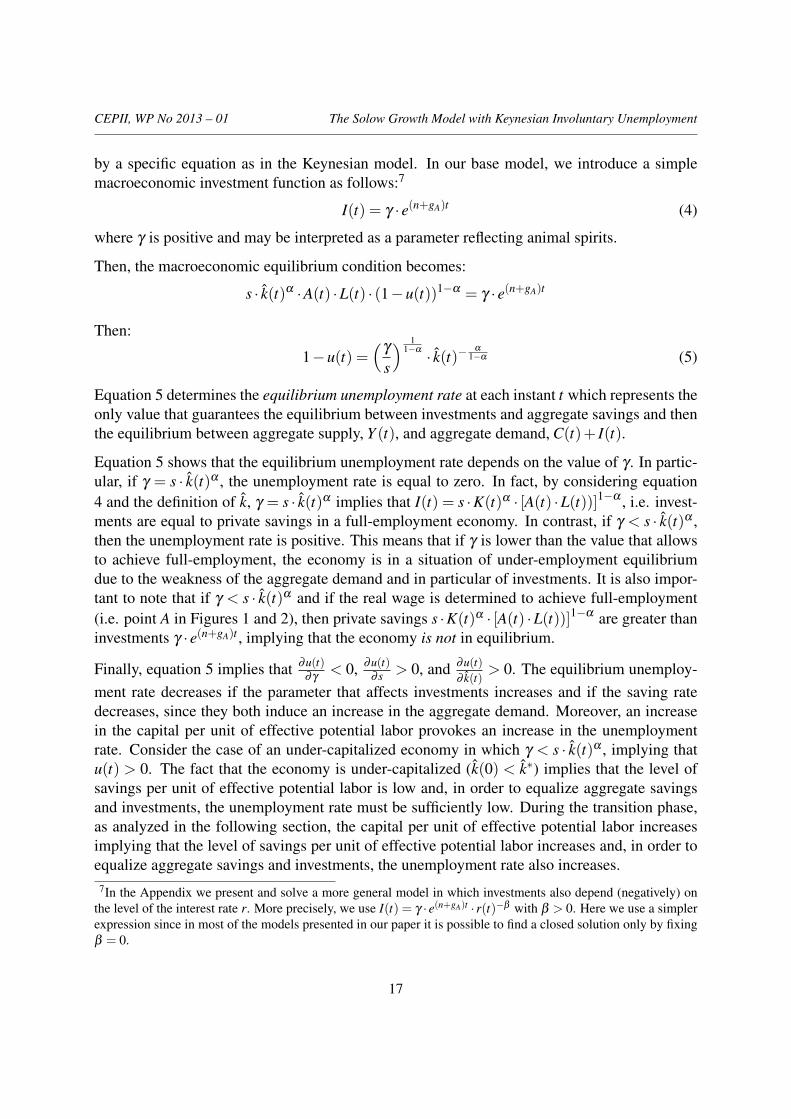
by a specific equation as in the Keynesian model. In our base model, we introduce a simplemacroeconomic investment function as follows:7
I(t) = γ · e(n+gA)t (4)
where γ is positive and may be interpreted as a parameter reflecting animal spirits.
Then, the macroeconomic equilibrium condition becomes:
s · k(t)α ·A(t) ·L(t) · (1−u(t))1−α = γ · e(n+gA)t
Then:
1−u(t) =(
γ
s
) 11−α · k(t)−
α
1−α (5)
Equation 5 determines the equilibrium unemployment rate at each instant t which represents theonly value that guarantees the equilibrium between investments and aggregate savings and thenthe equilibrium between aggregate supply, Y (t), and aggregate demand, C(t)+ I(t).
Equation 5 shows that the equilibrium unemployment rate depends on the value of γ . In partic-ular, if γ = s · k(t)α , the unemployment rate is equal to zero. In fact, by considering equation4 and the definition of k, γ = s · k(t)α implies that I(t) = s ·K(t)α · [A(t) ·L(t))]1−α , i.e. invest-ments are equal to private savings in a full-employment economy. In contrast, if γ < s · k(t)α ,then the unemployment rate is positive. This means that if γ is lower than the value that allowsto achieve full-employment, the economy is in a situation of under-employment equilibriumdue to the weakness of the aggregate demand and in particular of investments. It is also impor-tant to note that if γ < s · k(t)α and if the real wage is determined to achieve full-employment(i.e. point A in Figures 1 and 2), then private savings s ·K(t)α · [A(t) ·L(t))]1−α are greater thaninvestments γ · e(n+gA)t , implying that the economy is not in equilibrium.
Finally, equation 5 implies that ∂u(t)∂γ
< 0, ∂u(t)∂ s > 0, and ∂u(t)
∂ k(t)> 0. The equilibrium unemploy-
ment rate decreases if the parameter that affects investments increases and if the saving ratedecreases, since they both induce an increase in the aggregate demand. Moreover, an increasein the capital per unit of effective potential labor provokes an increase in the unemploymentrate. Consider the case of an under-capitalized economy in which γ < s · k(t)α , implying thatu(t) > 0. The fact that the economy is under-capitalized (k(0) < k∗) implies that the level ofsavings per unit of effective potential labor is low and, in order to equalize aggregate savingsand investments, the unemployment rate must be sufficiently low. During the transition phase,as analyzed in the following section, the capital per unit of effective potential labor increasesimplying that the level of savings per unit of effective potential labor increases and, in order toequalize aggregate savings and investments, the unemployment rate also increases.
7In the Appendix we present and solve a more general model in which investments also depend (negatively) onthe level of the interest rate r. More precisely, we use I(t) = γ · e(n+gA)t · r(t)−β with β > 0. Here we use a simplerexpression since in most of the models presented in our paper it is possible to find a closed solution only by fixingβ = 0.
17
CEPII, WP No 2013 – 01 The Solow Growth Model with Keynesian Involuntary Unemployment
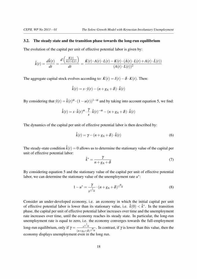
3.2. The steady state and the transition phase towards the long-run equilibrium
The evolution of the capital per unit of effective potential labor is given by:
˙k(t) =dk(t)
dt=
d(
K(t)A(t)·L(t)
)dt
=K(t) ·A(t) ·L(t)−K(t) · (A(t) ·L(t)+A(t) · L(t))
(A(t) ·L(t))2
The aggregate capital stock evolves according to: K(t) = I(t)−δ ·K(t). Then:
˙k(t) = s · y(t)− (n+gA +δ ) · k(t)
By considering that y(t) = k(t)α · (1−u(t))1−α and by taking into account equation 5, we find:
˙k(t) = s · k(t)α · γs· k(t)−α − (n+gA +δ ) · k(t)
The dynamics of the capital per unit of effective potential labor is then described by:
˙k(t) = γ− (n+gA +δ ) · k(t) (6)
The steady-state condition ˙k(t) = 0 allows us to determine the stationary value of the capital perunit of effective potential labor:
k∗ =γ
n+gA +δ(7)
By considering equation 5 and the stationary value of the capital per unit of effective potentiallabor, we can determine the stationary value of the unemployment rate u∗:
1−u∗ =γ
s1
1−α
· (n+gA +δ )α
1−α (8)
Consider an under-developed economy, i.e. an economy in which the initial capital per unitof effective potential labor is lower than its stationary value, i.e. k(0) < k∗. In the transitionphase, the capital per unit of effective potential labor increases over time and the unemploymentrate increases over time, until the economy reaches its steady state. In particular, the long-rununemployment rate is equal to zero, i.e. the economy converges towards the full-employment
long-run equilibrium, only if γ = s1
1−α
(n+gA+δ )α
1−α
. In contrast, if γ is lower than this value, then the
economy displays unemployment even in the long run.
18
CEPII, WP No 2013 – 01 The Solow Growth Model with Keynesian Involuntary Unemployment
3.3. The effect of a change in the saving rate
Consider now an increase in the saving rate. If the increase in the saving rate is not accompaniedby an increase in the parameter γ , the steady state value of the capital per unit of effectivepotential labor remains unchanged (∂ k∗
∂ s = 0), while the unemployment rate increases (∂ (1−u∗)∂ s <
0).
The direct effect of an increase in the saving rate is a reduction in private consumption and,if investments do not increase to compensate the reduction in private consumption, the shortrun effect is a reduction in the aggregate demand and in real GDP, and then an increase inunemployment. If we consider the dynamics, the increase in the saving rate permits a greatercapital accumulation. However, the unemployment rate remains greater than before the shock.By considering that real GDP is given by Y (t) = k(t)α · (1− u(t))1−α ·A(t) · L(t), the short-run effect is negative since k(t) is a predetermined variable and u(t) increases. The long-runeffect is also negative since a change in the saving rate has no effect on k∗ (see equation 7)and increases the unemployment rate (see equation 8). Of course, this result is due to the factthat the specification of the investment function (see equation 4) implies that an increase in thesaving rate produces no effect on investments. This assumption is relaxed in the next section.
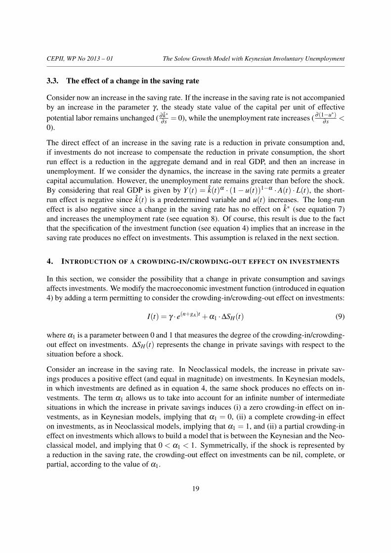
4. INTRODUCTION OF A CROWDING-IN/CROWDING-OUT EFFECT ON INVESTMENTS
In this section, we consider the possibility that a change in private consumption and savingsaffects investments. We modify the macroeconomic investment function (introduced in equation4) by adding a term permitting to consider the crowding-in/crowding-out effect on investments:
I(t) = γ · e(n+gA)t +α1 ·∆SH(t) (9)
where α1 is a parameter between 0 and 1 that measures the degree of the crowding-in/crowding-out effect on investments. ∆SH(t) represents the change in private savings with respect to thesituation before a shock.
Consider an increase in the saving rate. In Neoclassical models, the increase in private sav-ings produces a positive effect (and equal in magnitude) on investments. In Keynesian models,in which investments are defined as in equation 4, the same shock produces no effects on in-vestments. The term α1 allows us to take into account for an infinite number of intermediatesituations in which the increase in private savings induces (i) a zero crowding-in effect on in-vestments, as in Keynesian models, implying that α1 = 0, (ii) a complete crowding-in effecton investments, as in Neoclassical models, implying that α1 = 1, and (ii) a partial crowding-ineffect on investments which allows to build a model that is between the Keynesian and the Neo-classical model, and implying that 0 < α1 < 1. Symmetrically, if the shock is represented bya reduction in the saving rate, the crowding-out effect on investments can be nil, complete, orpartial, according to the value of α1.
19
CEPII, WP No 2013 – 01 The Solow Growth Model with Keynesian Involuntary Unemployment
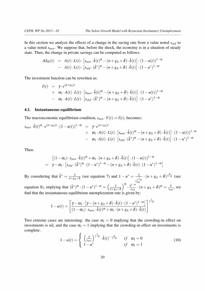
In this section we analyze the effects of a change in the saving rate from a value noted sold toa value noted snew. We suppose that, before the shock, the economy is in a situation of steadystate. Then, the change in private savings can be computed as follows:
∆SH(t) = A(t) ·L(t) ·[snew · k(t)α − (n+gA +δ ) · k(t)
]· (1−u(t))1−α
− A(t) ·L(t) ·[sold · (k∗)α − (n+gA +δ ) · k(t)
]· (1−u∗)1−α
The investment function can be rewritten as:
I(t) = γ · e(n+gA)t
+ α1 ·A(t) ·L(t) ·[snew · k(t)α − (n+gA +δ ) · k(t)
]· (1−u(t))1−α
− α1 ·A(t) ·L(t) ·[sold · (k∗)α − (n+gA +δ ) · k(t)
]· (1−u∗)1−α
4.1. Instantaneous equilibrium
The macroeconomic equilibrium condition, snew ·Y (t) = I(t), becomes:
snew · k(t)α · e(n+gA)t · (1−u(t))1−α = γ · e(n+gA)t
+ α1 ·A(t) ·L(t) ·[snew · k(t)α − (n+gA +δ ) · k(t)
]· (1−u(t))1−α
− α1 ·A(t) ·L(t) ·[sold · (k∗)α − (n+gA +δ ) · k(t)
]· (1−u∗)1−α
Then: [(1−α1) · snew · k(t)α +α1 · (n+gA +δ ) · k(t)
]· (1−u(t))1−α
= γ−α1 ·[sold · (k∗)α · (1−u∗)1−α − (n+gA +δ ) · k(t) · (1−u∗)1−α
]By considering that k∗ = γ
n+gA+δ(see equation 7) and 1− u∗ = γ
s1
1−α
old
· (n+ gA + δ )α
1−α (see
equation 8), implying that (k∗)α · (1− u∗)1−α =(
γ
n+gA+δ
)α
· γ1−α
sold· (n+ gA + δ )α = γ
sold, we
find that the instantaneous equilibrium unemployment rate is given by:
1−u(t) =
[γ−α1 ·
[γ− (n+gA +δ ) · k(t) · (1−u∗)1−α
](1−α1) · snew · k(t)α +α1 · (n+gA +δ ) · k(t)
] 11−α
Two extreme cases are interesting: the case α1 = 0 implying that the crowding-in effect oninvestments is nil, and the case α1 = 1 implying that the crowding-in effect on investments iscomplete:
1−u(t) =
(
γ
snew
) 11−α · k(t)−
α
1−α i f α1 = 01−u∗ i f α1 = 1
(10)
20
CEPII, WP No 2013 – 01 The Solow Growth Model with Keynesian Involuntary Unemployment
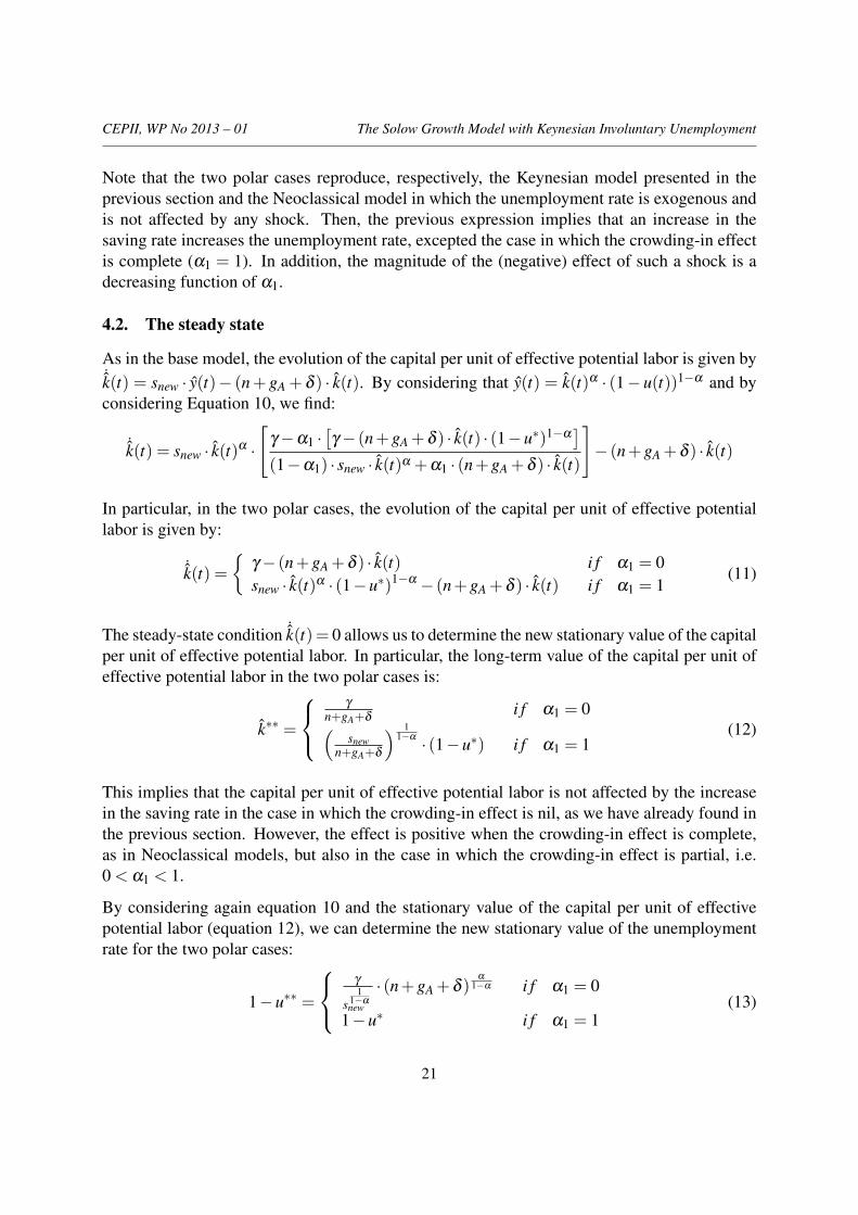
Note that the two polar cases reproduce, respectively, the Keynesian model presented in theprevious section and the Neoclassical model in which the unemployment rate is exogenous andis not affected by any shock. Then, the previous expression implies that an increase in thesaving rate increases the unemployment rate, excepted the case in which the crowding-in effectis complete (α1 = 1). In addition, the magnitude of the (negative) effect of such a shock is adecreasing function of α1.
4.2. The steady state
As in the base model, the evolution of the capital per unit of effective potential labor is given by˙k(t) = snew · y(t)− (n+ gA + δ ) · k(t). By considering that y(t) = k(t)α · (1− u(t))1−α and byconsidering Equation 10, we find:
˙k(t) = snew · k(t)α ·
[γ−α1 ·
[γ− (n+gA +δ ) · k(t) · (1−u∗)1−α
](1−α1) · snew · k(t)α +α1 · (n+gA +δ ) · k(t)
]− (n+gA +δ ) · k(t)
In particular, in the two polar cases, the evolution of the capital per unit of effective potentiallabor is given by:
˙k(t) ={
γ− (n+gA +δ ) · k(t) i f α1 = 0snew · k(t)α · (1−u∗)1−α − (n+gA +δ ) · k(t) i f α1 = 1
(11)
The steady-state condition ˙k(t)= 0 allows us to determine the new stationary value of the capitalper unit of effective potential labor. In particular, the long-term value of the capital per unit ofeffective potential labor in the two polar cases is:
k∗∗ =
γ
n+gA+δi f α1 = 0(
snewn+gA+δ
) 11−α · (1−u∗) i f α1 = 1
(12)
This implies that the capital per unit of effective potential labor is not affected by the increasein the saving rate in the case in which the crowding-in effect is nil, as we have already found inthe previous section. However, the effect is positive when the crowding-in effect is complete,as in Neoclassical models, but also in the case in which the crowding-in effect is partial, i.e.0 < α1 < 1.
By considering again equation 10 and the stationary value of the capital per unit of effectivepotential labor (equation 12), we can determine the new stationary value of the unemploymentrate for the two polar cases:
1−u∗∗ =
γ
s1
1−αnew
· (n+gA +δ )α
1−α i f α1 = 0
1−u∗ i f α1 = 1(13)
21
CEPII, WP No 2013 – 01 The Solow Growth Model with Keynesian Involuntary Unemployment
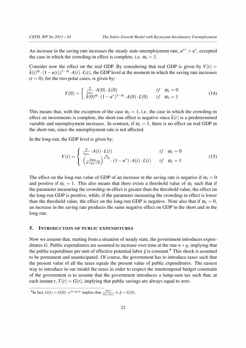
An increase in the saving rate increases the steady state unemployment rate, u∗∗ > u∗, exceptedthe case in which the crowding-in effect is complete, i.e. α1 = 1.
Consider now the effect on the real GDP. By considering that real GDP is given by Y (t) =k(t)α ·(1−u(t))1−α ·A(t) ·L(t), the GDP level at the moment in which the saving rate increases(t = 0), for the two polar cases, is given by:
Y (0) ={ γ
snew·A(0) ·L(0) i f α1 = 0
k(0)α · (1−u∗)1−α ·A(0) ·L(0) i f α1 = 1(14)
This means that, with the exception of the case α1 = 1, i.e. the case in which the crowding-ineffect on investments is complete, the short-run effect is negative since k(t) is a predeterminedvariable and unemployment increases. In contrast, if α1 = 1, there is no effect on real GDP inthe short-run, since the unemployment rate is not affected.
In the long-run, the GDP level is given by:
Y (t) =
γ
snew·A(t) ·L(t) i f α1 = 0(snew
n+gA+δ
) α
1−α · (1−u∗) ·A(t) ·L(t) i f α1 = 1(15)
The effect on the long-run value of GDP of an increase in the saving rate is negative if α1 = 0and positive if α1 = 1. This also means that there exists a threshold value of α1 such that ifthe parameter measuring the crowding-in effect is greater than the threshold value, the effect onthe long-run GDP is positive, while, if the parameter measuring the crowding-in effect is lowerthan the threshold value, the effect on the long-run GDP is negative. Note also that if α1 = 0,an increase in the saving rate produces the same negative effect on GDP in the short and in thelong run.
5. INTRODUCTION OF PUBLIC EXPENDITURES
Now we assume that, starting from a situation of steady state, the government introduces expen-ditures G. Public expenditures are assumed to increase over time at the rate n+g, implying thatthe public expenditure per unit of effective potential labor g is constant.8 This shock is assumedto be permanent and unanticipated. Of course, the government has to introduce taxes such thatthe present value of all the taxes equals the present value of public expenditures. The easiestway to introduce in our model the taxes in order to respect the intertemporal budget constraintof the government is to assume that the government introduces a lump-sum tax such that, ateach instant t, T (t) = G(t), implying that public savings are always equal to zero.
8In fact, G(t) = G(0) · e(n+gA)t implies that G(t)A(t)·L(t) ≡ g = G(0).
22
CEPII, WP No 2013 – 01 The Solow Growth Model with Keynesian Involuntary Unemployment
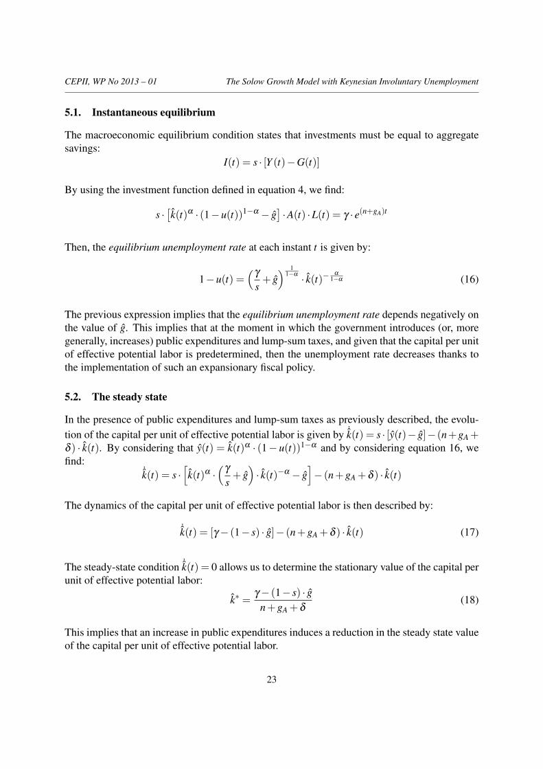
5.1. Instantaneous equilibrium
The macroeconomic equilibrium condition states that investments must be equal to aggregatesavings:
I(t) = s · [Y (t)−G(t)]
By using the investment function defined in equation 4, we find:
s ·[k(t)α · (1−u(t))1−α − g
]·A(t) ·L(t) = γ · e(n+gA)t
Then, the equilibrium unemployment rate at each instant t is given by:
1−u(t) =(
γ
s+ g) 1
1−α · k(t)−α
1−α (16)
The previous expression implies that the equilibrium unemployment rate depends negatively onthe value of g. This implies that at the moment in which the government introduces (or, moregenerally, increases) public expenditures and lump-sum taxes, and given that the capital per unitof effective potential labor is predetermined, then the unemployment rate decreases thanks tothe implementation of such an expansionary fiscal policy.
5.2. The steady state
In the presence of public expenditures and lump-sum taxes as previously described, the evolu-tion of the capital per unit of effective potential labor is given by ˙k(t) = s · [y(t)− g]− (n+gA+δ ) · k(t). By considering that y(t) = k(t)α · (1− u(t))1−α and by considering equation 16, wefind:
˙k(t) = s ·[k(t)α ·
(γ
s+ g)· k(t)−α − g
]− (n+gA +δ ) · k(t)
The dynamics of the capital per unit of effective potential labor is then described by:
˙k(t) = [γ− (1− s) · g]− (n+gA +δ ) · k(t) (17)
The steady-state condition ˙k(t) = 0 allows us to determine the stationary value of the capital perunit of effective potential labor:
k∗ =γ− (1− s) · g
n+gA +δ(18)
This implies that an increase in public expenditures induces a reduction in the steady state valueof the capital per unit of effective potential labor.
23
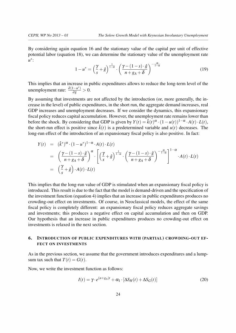
CEPII, WP No 2013 – 01 The Solow Growth Model with Keynesian Involuntary Unemployment
By considering again equation 16 and the stationary value of the capital per unit of effectivepotential labor (equation 18), we can determine the stationary value of the unemployment rateu∗:
1−u∗ =(
γ
s+ g) 1
1−α ·(
γ− (1− s) · gn+gA +δ
)− α
1−α
(19)
This implies that an increase in public expenditures allows to reduce the long-term level of theunemployment rate: ∂ (1−u∗)
∂ g > 0.
By assuming that investments are not affected by the introduction (or, more generally, the in-crease in the level) of public expenditures, in the short run, the aggregate demand increases, realGDP increases and unemployment decreases. If we consider the dynamics, this expansionaryfiscal policy reduces capital accumulation. However, the unemployment rate remains lower thanbefore the shock. By considering that GDP is given by Y (t) = k(t)α · (1−u(t))1−α ·A(t) ·L(t),the short-run effect is positive since k(t) is a predetermined variable and u(t) decreases. Thelong-run effect of the introduction of an expansionary fiscal policy is also positive. In fact:
Y (t) = (k∗)α · (1−u∗)1−α ·A(t) ·L(t)
=
(γ− (1− s) · g
n+gA +δ
)α
·
[(γ
s+ g) 1
1−α ·(
γ− (1− s) · gn+gA +δ
)− α
1−α
]1−α
·A(t) ·L(t)
=(
γ
s+ g)·A(t) ·L(t)
This implies that the long-run value of GDP is stimulated when an expansionary fiscal policy isintroduced. This result is due to the fact that the model is demand-driven and the specification ofthe investment function (equation 4) implies that an increase in public expenditures produces nocrowding-out effect on investments. Of course, in Neoclassical models, the effect of the samefiscal policy is completely different: an expansionary fiscal policy reduces aggregate savingsand investments; this produces a negative effect on capital accumulation and then on GDP.Our hypothesis that an increase in public expenditures produces no crowding-out effect oninvestments is relaxed in the next section.
6. INTRODUCTION OF PUBLIC EXPENDITURES WITH (PARTIAL) CROWDING-OUT EF-FECT ON INVESTMENTS
As in the previous section, we assume that the government introduces expenditures and a lump-sum tax such that T (t) = G(t).
Now, we write the investment function as follows:
I(t) = γ · e(n+gA)t +α1 · [∆SH(t)+∆SG(t)] (20)
24
CEPII, WP No 2013 – 01 The Solow Growth Model with Keynesian Involuntary Unemployment
where α1 is again a parameter between 0 and 1 that measures the degree of the crowding-in/crowding-out effect on investments, ∆SH(t) represents the change in private savings withrespect to the situation before a shock, and ∆SG(t) represents the change in public savings withrespect to the situation before a shock. The investment function defined in equation 20 allowsto take into account for the crowding-out effect provoked by an increase in public expenditures.
Starting from a situation of steady state, the introduction of public expenditures, accompaniedby the introduction of a lump-sum tax such that T (t) = G(t), has no effect on public savings(∆SG(t) = 0) and produces the following change in private savings:
∆SH(t) =[s ·(k(t)α · (1−u(t))1−α − g
)− (n+gA +δ ) · k(t)
]·A(t) ·L(t)
−[s · (k∗)α − (n+gA +δ ) · k(t)
]· (1−u∗)1−α ·A(t) ·L(t)
6.1. Instantaneous equilibrium
The macroeconomic equilibrium condition can be written as follows:
s ·[k(t)α · (1−u(t))1−α − g
]= γ
+ α1 ·[s ·(k(t)α · (1−u(t))1−α − g
)− (n+gA +δ ) · k(t)
]− α1 ·
[s · (k∗)α − (n+gA +δ ) · k(t)
]· (1−u∗)1−α
Then: [(1−α1) · s · k(t)α +α1 · (n+gA +δ ) · k(t)
]· (1−u(t))1−α
= γ + s · (1−α1) · g−α1 ·[s · (k∗)α · (1−u∗)1−α − (n+gA +δ ) · k(t) · (1−u∗)1−α
]By considering that, without public expenditures, k∗ = γ
n+gA+δ(see equation 7) and 1− u∗ =
γ
s1
1−α
· (n+gA +δ )α
1−α (see equation 8), implying that (k∗)α · (1−u∗)1−α = γ
s , we find that the
instantaneous equilibrium unemployment rate is given by:
1−u(t) =
[γ + s · (1−α1) · g−α1 ·
[γ− (n+gA +δ ) · k(t) · (1−u∗)1−α
](1−α1) · s · k(t)α +α1 · (n+gA +δ ) · k(t)
] 11−α
(21)
In particular, the unemployment rate in the two polar cases is:
1−u(t) =
{ (γ
s + g) 1
1−α · k(t)α
1−α i f α1 = 01−u∗ i f α1 = 1
(22)
The previous expression implies that the introduction of public expenditures, accompanied bya simultaneous introduction of a lump-sum tax, permits to reduce the level of unemployment,excepted in the case α1 = 1.
25
CEPII, WP No 2013 – 01 The Solow Growth Model with Keynesian Involuntary Unemployment
6.2. The steady state
The introduction of public expenditures and lump-sum taxes as previously described, impliesthat the evolution of the capital per unit of effective potential labor is given by ˙k(t) = s · [y(t)−g]− (n+ gA + δ ) · k(t). By considering that y(t) = k(t)α · (1− u(t))1−α and by consideringequation 21, the dynamics of the capital per unit of effective potential labor is described by:
˙k(t) = s ·
[k(t)α ·
γ + s · (1−α1) · g−α1 ·[γ− (n+gA +δ ) · k(t) · (1−u∗)1−α
](1−α1) · s · k(t)α +α1 · (n+gA +δ ) · k(t)
− g
]− (n+gA +δ ) · k(t)
In particular, in the two polar cases, the evolution of the capital per unit of effective potentiallabor is given by:
˙k(t) =
{(γ +(1− s) · g)− (n+gA +δ ) · k(t) i f α1 = 0
s ·[k(t)α · (1−u∗)1−α − g
]− (n+gA +δ ) · k(t) i f α1 = 1
(23)
The steady-state condition, ˙k(t) = 0, allows us to determine the new stationary value of thecapital per unit of effective potential labor. It is possible to determine a closed solution for thelong-term value of the capital per unit of effective potential labor only if α1 = 0. In any cases,the long-term value of the capital per unit of effective potential labor is negatively affected bythe introduction of public expenditures. In the case of α1 = 0, the new stationary value of thecapital per unit of effective potential labor is:
k∗∗ ={
γ−(1−s)·gn+gA+δ
i f α1 = 0 (24)
By considering again equation 21 and the stationary value of the capital per unit of effectivepotential labor (equation 24), we can determine the new stationary value of the unemploymentrate for the two polar cases:
1−u∗∗ =
{γ−·g
s1
1−α
· (n+gA +δ )α
1−α i f α1 = 0
1−u∗ i f α1 = 1(25)
This implies that the expansionary fiscal policy permits a reduction of the long-term unemploy-ment rate, excepted in the case α1 = 1.
26
CEPII, WP No 2013 – 01 The Solow Growth Model with Keynesian Involuntary Unemployment
7. NUMERICAL SIMULATIONS
In this section we present numerical simulations in order to analyze the evolution of (i) anunder-developed economy, (ii) of an economy in which the saving rate increases, and (iii) aneconomy in which public expenditures are introduced.
We first calibrate our model at the steady state without public expenditures and taxes. Oureconomy is characterized by a population growth rate (n) of 0.5%, a productivity growth rate(g) of 1.5%, and a depreciation rate (δ ) of 4%. Moreover, α in the Cobb-Douglas productionfunction is fixed at 1/3, the saving rate (s) is equal to 20% and the parameter γ in the investmentequation has been calibrated in order to obtain a stationary unemployment rate equal to 10%.
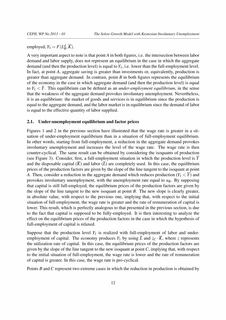
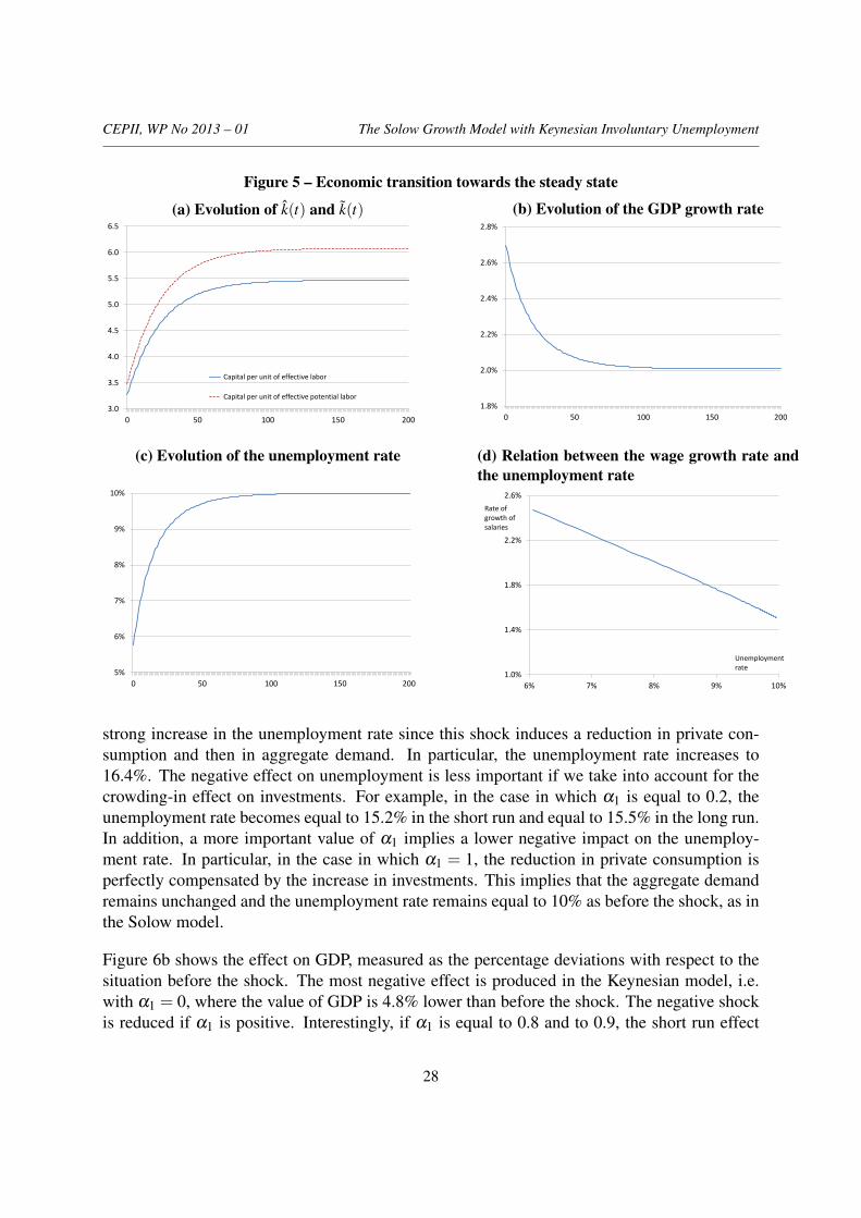
7.1. Transition of an under-capitalized economy
In the first simulation, we assume that the initial capital per unit of effective labor is equal to60% of the long-run value, implying that the economy is under-capitalized. Figure 5 showsthe economic transition towards the steady state. In particular, the evolution of the capitalper unit of effective labor and per unit of effective potential labor is presented in Figure 5a,the rate of growth of real GDP in Figure 5b, and the unemployment rate in Figure 5c. Thesimulation results indicate that the under-developed economy converges towards the steadystate. In particular, the unemployment rate increases over time from an initial value of 5.8%to the long-run value of 10%. One interesting aspect of this simulation is the relation betweenthe growth rate of real wages and the unemployment rate. Figure 5d shows the negative relationbetween these two variables that is coherent with the Phillips curve.9
7.2. Increase in the saving rate
In the second simulation we assume that the economy is already at the steady state and that theprivate saving rate increases from 20% to 21%.
We first solve the model using the Solow model, i.e. by assuming that investments are deter-mined by aggregate savings instead of by the investment function defined in equation 4 and byfixing the unemployment rate at 10% or, equivalently, by assuming that the number of workersis equal, at each period, to 90% of the active population. Then, we solve the model by intro-ducing equation 4 and by endogenizing the unemployment rate. Finally, we solve the model byconsidering different values of α1, i.e. different degrees of the crowding-in/crowding-out effecton investments.
The results are reported in Figure 6. In particular, Figure 6a shows the effect on the unemploy-ment rate. In the Keynesian model, i.e. with α1 = 0, the increase in the saving rate produces a
9The curve presented in Figure 5d coincides with the traditional Phillips curve only if the inflation rate is equal tozero. However, if the inflation rate is constant or sufficiently stable over time, the curve representing the relationbetween the growth rate of nominal wages and the unemployment rate is the same as the one depicted in Figure5d, with the only difference that it is shifted upward.
27
CEPII, WP No 2013 – 01 The Solow Growth Model with Keynesian Involuntary Unemployment
Figure 5 – Economic transition towards the steady state
(a) Evolution of k(t) and k(t)
3.0
3.5
4.0
4.5
5.0
5.5
6.0
6.5
0 50 100 150 200
Capital per unit of effective labor
Capital per unit of effective potential labor
(b) Evolution of the GDP growth rate
1.8%
2.0%
2.2%
2.4%
2.6%
2.8%
0 50 100 150 200
(c) Evolution of the unemployment rate
5%
6%
7%
8%
9%
10%
0 50 100 150 200
(d) Relation between the wage growth rate andthe unemployment rate
1.0%
1.4%
1.8%
2.2%
2.6%
6% 7% 8% 9% 10%
Rate of growth of salaries
Unemployment rate
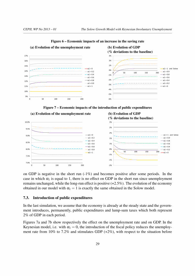
strong increase in the unemployment rate since this shock induces a reduction in private con-sumption and then in aggregate demand. In particular, the unemployment rate increases to16.4%. The negative effect on unemployment is less important if we take into account for thecrowding-in effect on investments. For example, in the case in which α1 is equal to 0.2, theunemployment rate becomes equal to 15.2% in the short run and equal to 15.5% in the long run.In addition, a more important value of α1 implies a lower negative impact on the unemploy-ment rate. In particular, in the case in which α1 = 1, the reduction in private consumption isperfectly compensated by the increase in investments. This implies that the aggregate demandremains unchanged and the unemployment rate remains equal to 10% as before the shock, as inthe Solow model.
Figure 6b shows the effect on GDP, measured as the percentage deviations with respect to thesituation before the shock. The most negative effect is produced in the Keynesian model, i.e.with α1 = 0, where the value of GDP is 4.8% lower than before the shock. The negative shockis reduced if α1 is positive. Interestingly, if α1 is equal to 0.8 and to 0.9, the short run effect
28
CEPII, WP No 2013 – 01 The Solow Growth Model with Keynesian Involuntary Unemployment
Figure 6 – Economic impacts of an increase in the saving rate
(a) Evolution of the unemployment rate
9%
10%
11%
12%
13%
14%
15%
16%
17%
0 50 100 150 200
α1 = 0
α1 = 0.2
α1 = 0.4
α1 = 0.6
α1 = 0.8
α1 = 0.9
α1 = 1
(b) Evolution of GDP(% deviations to the baseline)
-6%
-5%
-4%
-3%
-2%
-1%
0%
1%
2%
3%
0 50 100 150 200
α1 = 1 and Solow
α1 = 0.9
α1 = 0.8
α1 = 0.6
α1 = 0.4
α1 = 0.2
α1 = 0
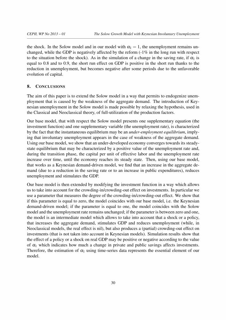
Figure 7 – Economic impacts of the introduction of public expenditures
(a) Evolution of the unemployment rate
7.0%
7.5%
8.0%
8.5%
9.0%
9.5%
10.0%
0 50 100 150 200
α1 = 0
α1 = 0.2
α1 = 0.4
α1 = 0.6
α1 = 0.8
α1 = 0.9
α1 = 1
(b) Evolution of GDP(% deviations to the baseline)
-2%
-1%
-1%
0%
1%
1%
2%
2%
3%
0 50 100 150 200
α1 = 1 and Solow
α1 = 0.9
α1 = 0.8
α1 = 0.6
α1 = 0.4
α1 = 0.2
α1 = 0
on GDP is negative in the short run (-1%) and becomes positive after some periods. In thecase in which α1 is equal to 1, there is no effect on GDP in the short run since unemploymentremains unchanged, while the long-run effect is positive (+2.5%). The evolution of the economyobtained in our model with α1 = 1 is exactly the same obtained in the Solow model.
7.3. Introduction of public expenditures
In the last simulation, we assume that the economy is already at the steady state and the govern-ment introduces, permanently, public expenditures and lump-sum taxes which both represent2% of GDP in each period.
Figures 7a and 7b show respectively the effect on the unemployment rate and on GDP. In theKeynesian model, i.e. with α1 = 0, the introduction of the fiscal policy reduces the unemploy-ment rate from 10% to 7.2% and stimulates GDP (+2%), with respect to the situation before
29
CEPII, WP No 2013 – 01 The Solow Growth Model with Keynesian Involuntary Unemployment
the shock. In the Solow model and in our model with α1 = 1, the unemployment remains un-changed, while the GDP is negatively affected by the reform (-1% in the long run with respectto the situation before the shock). As in the simulation of a change in the saving rate, if α1 isequal to 0.8 and to 0.9, the short run effect on GDP is positive in the short run thanks to thereduction in unemployment, but becomes negative after some periods due to the unfavorableevolution of capital.
8. CONCLUSIONS
The aim of this paper is to extend the Solow model in a way that permits to endogenize unem-ployment that is caused by the weakness of the aggregate demand. The introduction of Key-nesian unemployment in the Solow model is made possible by relaxing the hypothesis, used inthe Classical and Neoclassical theory, of full-utilization of the production factors.
Our base model, that with respect the Solow model presents one supplementary equation (theinvestment function) and one supplementary variable (the unemployment rate), is characterizedby the fact that the instantaneous equilibrium may be an under-employment equilibrium, imply-ing that involuntary unemployment appears in the case of weakness of the aggregate demand.Using our base model, we show that an under-developed economy converges towards its steady-state equilibrium that may be characterized by a positive value of the unemployment rate and,during the transition phase, the capital per unit of effective labor and the unemployment rateincrease over time, until the economy reaches its steady state. Then, using our base model,that works as a Keynesian demand-driven model, we find that an increase in the aggregate de-mand (due to a reduction in the saving rate or to an increase in public expenditures), reducesunemployment and stimulates the GDP.
Our base model is then extended by modifying the investment function in a way which allowsus to take into account for the crowding-in/crowding-out effect on investments. In particular weuse a parameter that measures the degree of the crowding-in/crowding-out effect. We show thatif this parameter is equal to zero, the model coincides with our base model, i.e. the Keynesiandemand-driven model; if the parameter is equal to one, the model coincides with the Solowmodel and the unemployment rate remains unchanged; if the parameter is between zero and one,the model is an intermediate model which allows to take into account that a shock or a policy,that increases the aggregate demand, stimulates GDP and reduces unemployment (while, inNeoclassical models, the real effect is nil), but also produces a (partial) crowding-out effect oninvestments (that is not taken into account in Keynesian models). Simulation results show thatthe effect of a policy or a shock on real GDP may be positive or negative according to the valueof α1 which indicates how much a change in private and public savings affects investments.Therefore, the estimation of α1 using time-series data represents the essential element of ourmodel.
30
CEPII, WP No 2013 – 01 The Solow Growth Model with Keynesian Involuntary Unemployment
REFERENCES
Backhouse, Roger E., (1981), Keynesian Unemployment and the One-Sector Neoclassical Growth Model,Economic Journal, 91, issue 361, p. 174-87.
Barro, Robert J. and Grossman, Herschel., (1971), A General Disequilibrium Model of Income andEmployment, American Economic Review, 61, issue 1, p. 82-93.
Benassy, Jean-Pascal, (1975), Neo-Keynesian Disequilibrium Theory in a Monetary Economy, Reviewof Economic Studies, 42, issue 4, p. 503-23.
Chatterjee, Santanu, (2005), Capital Utilization, Economic Growth and Convergence, Journal of Eco-nomic Dynamics and Control, 29, issue 12, p. 2093-2124.
Clower, Robert, The Keynesian Counter-Revolution: a Theoretical Appraisal, in Hahn and Brechling,The Theory of Interest Rates, Macmillan, London, 1965, p. 103-125.
Davidson, Paul, (1967), A Keynesian View of Patinkin’s Theory of Employment, The Economic Journal,77, issue 307, p. 559-578.
Davidson, Paul, (1983), The Marginal Product Curve Is Not the Demand Curve for Labor and Lucas’sLabor Supply Function Is Not the Supply Curve for Labor in the Real World, Journal of Post KeynesianEconomics, 6, Issue 1, p. 105-117.
Keynes, John Maynard, (1936), The General Theory of Employment, Interest and Money, New York.
Leijonhufvud, Axel. (1968), On Keynesian Economics and the Economics of Keynes: A Study in Mone-tary Theory, New York: Oxford University Press.
Malinvaud, Edmond (1977), The Theory of Unemployment Reconsidered, Oxford, Basil Blackwell.
Mankiw, N. Gregory, (1989), Real Business Cycles: A New Keynesian Perspective, Journal of EconomicPerspectives, 3, issue 3, p. 79-90.
Patinkin, Don (1965), Money, Interest and Prices, 2nd edition. New York.
Solow, Robert, (1956), A Contribution to the Theory of Economic Growth, The Quarterly Journal ofEconomics, 70, issue 1, p. 65-94.
31
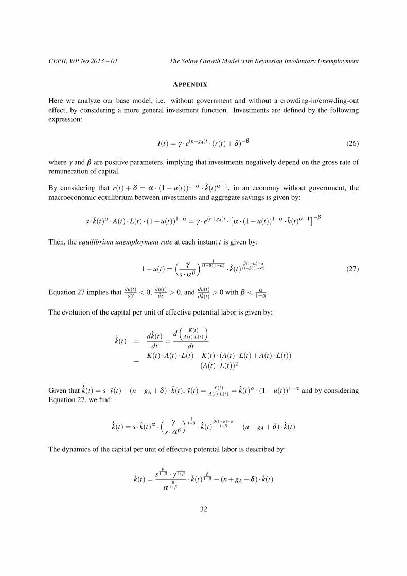
CEPII, WP No 2013 – 01 The Solow Growth Model with Keynesian Involuntary Unemployment
APPENDIX
Here we analyze our base model, i.e. without government and without a crowding-in/crowding-outeffect, by considering a more general investment function. Investments are defined by the followingexpression:
I(t) = γ · e(n+gA)t · (r(t)+δ )−β (26)
where γ and β are positive parameters, implying that investments negatively depend on the gross rate ofremuneration of capital.
By considering that r(t) + δ = α · (1− u(t))1−α · k(t)α−1, in an economy without government, themacroeconomic equilibrium between investments and aggregate savings is given by:
s · k(t)α ·A(t) ·L(t) · (1−u(t))1−α = γ · e(n+gA)t ·[α · (1−u(t))1−α · k(t)α−1]−β
Then, the equilibrium unemployment rate at each instant t is given by:
1−u(t) =(
γ
s ·αβ
) 1(1+β )(1−α) · k(t)
β (1−α)−α
(1+β )(1−α) (27)
Equation 27 implies that ∂u(t)∂γ
< 0, ∂u(t)∂ s > 0, and ∂u(t)
∂ k(t)> 0 with β < α
1−α.
The evolution of the capital per unit of effective potential labor is given by:
˙k(t) =dk(t)
dt=
d(
K(t)A(t)·L(t)
)dt
=K(t) ·A(t) ·L(t)−K(t) · (A(t) ·L(t)+A(t) · L(t))
(A(t) ·L(t))2
Given that ˙k(t) = s · y(t)− (n+gA + δ ) · k(t), y(t) = Y (t)A(t)·L(t) = k(t)α · (1−u(t))1−α and by considering
Equation 27, we find:
˙k(t) = s · k(t)α ·(
γ
s ·αβ
) 11+β · k(t)
β (1−α)−α
1+β − (n+gA +δ ) · k(t)
The dynamics of the capital per unit of effective potential labor is described by:
˙k(t) =s
β
1+β · γ1
1+β
αβ
1+β
· k(t)β
1+β − (n+gA +δ ) · k(t)
32
CEPII, WP No 2013 – 01 The Solow Growth Model with Keynesian Involuntary Unemployment
The steady-state condition ˙k(t) = 0 allows us to determine the stationary value of the capital per unit ofeffective potential labor:
k∗ =sβ · γ
αβ · (n+gA +δ )1+β(28)
By considering again equation 27 and the stationary value of the capital per unit of effective potentiallabor, we can determine the stationary value of the unemployment rate u∗:10
1−u∗ =γ
s ·αβ·(
sn+gA +δ
)β− α
1−α
(29)
The equilibrium exists, is unique,11 and is stable if β < 1.
In the transition phase, an under-developed economy with k(0) < k∗, the capital par unit of effectivepotential labor increase over time and, with β sufficiently low, the unemployment rate increases overtime, until the economy reaches its steady state.
10See the Appendix for the detailed computation.11Without taking into account for the case k∗ = 0.
33
CEPII, WP No 2013-01 The Salow Growth Model with kenesian Involuntary Unemployment
34
LIST OF WORKING PAPERS RELEASED BY CEPII
An Exhaustive list is available on the website: \\www.cepii.fr.
No Title Authors
2012-38 Does Migration Foster Exports? An African Perspective
H. Ehrhart, M. Le Goff,E. Rocher & R. J. Singh
2012-37 The ECB Unconventional Monetary Policies: Have they Lowered Market Borrowing Costs for Banks and Governments?
U. Szczerbowicz
2012-36 The Impact of Market Regulations on Intra-European Real Exchange Rages
A. Bénassy-Quéré& D. Coulibaly
2012-35 Exchange Rate volatility, Financial Constraints and Trade: Empirical Evidence from Chinese Firms
J. Héricourt & S. Poncet
2012-34 Multinational Retailers and Home Country Exports A. Cheptea, C. Emlinger& K. Latouche
2012-33 Food Prices and Inflation Targeting in Emerging Economies
M. Pourroy, B. Carton& D. Coulibaly
2012-32 Fiscal Consolidations and Banking Stability J. Cimadomo, S. Hauptmeier
& T. Zimmermann
2012-31 The Contribution of the Yen Appreciation since 2007 to the Japanese Economic Debacle
W. Thorbecke
2012-30 Are the Benefits of Exports Support Durable? O. Cadot,A. M. Fernandes,
J. Gourdon & A. Mattoo
CEPII, WP No 2013-01 The Salow Growth Model with kenesian Involuntary Unemployment
35
No Title Authors
2012-29 Les dessous de la dette publique japonaise E. Dourille-Feer
2012-28 Invoicing Currency, Firm Size, and Hedging J. Martin & I. Méjean
2012-27 Product Relatedness and Firm Exports in China S. Poncet & F. Starosta de Waldemar
2012-26 Export Upgrading and Growth: the Prerequisite of Domestic Embeddedness
S. Poncet & F. Starosta de Waldemar
2012-25 Time to Ship During Financial Crises N. Berman, J. de SousaP. Martin & T. Mayer
2012-24 Foreign Ownership Wage Premium: Does financial Health Matter?
M. Bas
2012-23 Tax Reform and Coordination in a Currency Union B. Carton
2012-22 The Unequal Effects of Financial Development on Firms’ Growth in India
M. Bas & A. Berthou
2012-21 Pegging Emerging Currencies in the Face of Dollar Swings
V. Coudert, C. Couharde& V. Mignon
2012-20 On the Links between Stock and Comodity Markets’ Volatility
A. Creti, M. Joëts& V. Mignon
2012-19 European Export Performance, Angela Cheptea A. Cheptea, L. Fontagné& S. Zignago
2012-18 The Few Leading the Many: Foreign Affiliates and Business Cycle Comovement
J. Kleinert, J. Martin& F. Toubal
2012-17 Native Language, Spoken Language, Translation and Trade
J. Melitz & F. Toubal
2012-16 Assessing the Price-Raising Effect of Non-Tariff Measures in Africa
O.Cadot & J.Gourdon
2012-15 International Migration and Trade Agreements: the New Role of PTAs
G. Orefice
CEPII, WP No 2013-01 The Salow Growth Model with kenesian Involuntary Unemployment
36
No Title Authors
2012-14 Scanning the Ups and Downs of China’s Trade Imbalances
F. Lemoine & D. Ünal
2012-13 Revisiting the Theory of Optimum Currency Areas: Is the CFA Franc Zone Sustainable?
C. Couharde, I. Coulibaly, D. Guerreiro
& V. Mignon
2012-12 Macroeconomic Transmission of Eurozone Shocks to Emerging Economies
B. Erten
2012-11 The fiscal Impact of Immigration in France: a Generational Accounting Approach
X. Chojnicki
2012-10 MAcMap-HS6 2007, an Exhaustive and Consistent Measure of Applied Protection in 2007
H. Guimbard, S. Jean,M. Mimouni & X. Pichot
2012-09 Regional Integration and Natural Resources: Who Benefits? Evidence from MENA
C. Carrère, J. Gourdon& M. Olarreaga
2012-08 A Foreign Direct Investment Database for Global CGE Models
C. Gouël, H. Guimbard& D. Laborde
2012-07 On Currency Misalignments within the Euro Area V. Coudert, C. Couharde & V. Mignon
2012-06 How Frequently Firms Export? Evidence from France G. Békés, L. Fontagné,B. Muraközy & V. Vicard
2012-05 Fiscal Sustainability in the Presence of Systemic Banks: the Case of EU Countries
A. Bénassy-Quéré& G. Roussellet
2012-04 Low-Wage Countries’ Competition, Reallocation across Firms and the Quality Content of Exports
J. Martin & I. Méjean
2012-03 The Great Shift: Macroeconomic Projections for the World Economy at the 2050 Horizon
J. Fouré,A. Bénassy-Quéré
& L. Fontagné
2012-02 The Discriminatory Effect of Domestic Regulations on International Services Trade: Evidence from Firm-Level Data
M. Crozet, E. Milet& D. Mirza

CEPII, WP No 2013-01 The Salow Growth Model with kenesian Involuntary Unemployment
37
No Title Authors
2012-01 Optimal food price stabilization in a small open developing country
C. Gouël & S. Jean

Organisme public d’étude et de recherche en économie internationale, le CEPII est placé auprès du Centre d’Analyse Stratégique. Son programme de travail est fixé par un conseil composé de responsables de l’administration et de personnalités issues des entreprises, des organisations syndicales et de l’Université.
Les documents de travail du CEPII mettent à disposition du public professionnel des travaux effectués au CEPII, dans leur phase d’élaboration et de discussion avant publication définitive. Les documents de travail sont publiés sous la responsabilité de la direction du CEPII et n’engagent ni le conseil du Centre, ni le Centre d’Analyse Stratégique. Les opinions qui y sont exprimées sont celles des auteurs.
Les documents de travail du CEPII sont disponibles sur le site : http//www.cepii.fr.