1

Economics 405 Linda KamasSanta Clara University April 22, 24, 2014 

  NOTES ON THE SIMPLE KEYNESIAN MODEL   I. Aggregate Demand or Planned Expenditure (Ep): Ep = C + Ip + G + NX  Aggregate demand or planned expenditure determines the level of GDP.  Aggregate demand and planned expenditure are the same thing. We will call it aggregate demand AD when we graph it with varying prices and aggregate expenditure when we ignore price changes. Firms respond to demand: Decrease in Aggregate Expenditure: excess supply of goods; firms see sales decline and inventories increase. They respond to undesired increase in inventories by decreasing production. GDP declines, employment declines. and unemployment rises. (Firms may also lower prices; we will cover this later.) Increase in Aggregate Expenditure: excess demand for goods; causes an undesired decline in inventories and firms respond by producing more and GDP increases, employment increases, and unemployment falls.

2

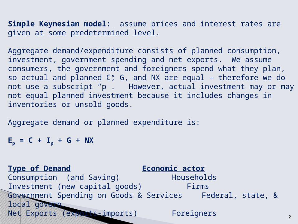
Simple Keynesian model: assume prices and interest rates are given at some predetermined level. Aggregate demand/expenditure consists of planned consumption, investment, government spending and net exports. We assume consumers, the government and foreigners spend what they plan, so actual and planned C, G, and NX are equal – therefore we do not use a subscript “p”. However, actual investment may or may not equal planned investment because it includes changes in inventories or unsold goods. Aggregate demand or planned expenditure is:

 Ep = C + Ip + G + NX  

Type of Demand Economic actorConsumption (and Saving) HouseholdsInvestment (new capital goods) FirmsGovernment Spending on Goods & Services Federal, state, & local govern.Net Exports (exports-imports) Foreigners

3

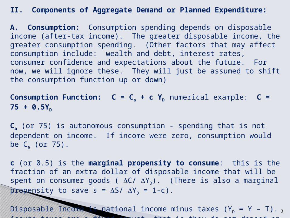
II. Components of Aggregate Demand or Planned Expenditure: A. Consumption: Consumption spending depends on disposable income (after-tax income). The greater disposable income, the greater consumption spending. (Other factors that may affect consumption include: wealth and debt, interest rates, consumer confidence and expectations about the future. For now, we will ignore these. They will just be assumed to shift the consumption function up or down)

Consumption Function: C = Ca + c YD numerical example: C = 75 + 0.5YD

 Ca (or 75) is autonomous consumption - spending that is not dependent on income. If income were zero, consumption would be Ca (or 75). c (or 0.5) is the marginal propensity to consume: this is the fraction of an extra dollar of disposable income that will be spent on consumer goods ( C/ YD). (There is also a marginal propensity to save s = S/ YD = 1-c). Disposable Income is national income minus taxes (YD = Y – T). Assume taxes are a fixed amount, that is they do not depend on income so they are autonomous:  Taxes: T = Ta Ta= 100. 

Consumption function is: C = Ca + c(Y-Ta) C = 75 + 0.5(Y - 100)

4

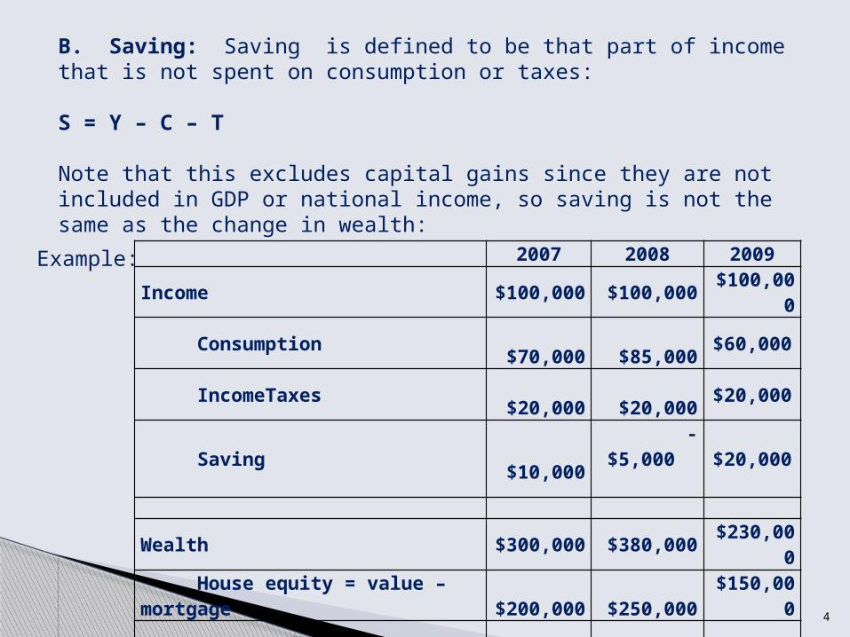
2007 2008 2009Income $100,000 $100,000 $100,000 Consumption $70,000 $85,000 $60,000 IncomeTaxes $20,000 $20,000 $20,000

Saving $10,000 - $5,000 $20,000

Wealth $300,000 $380,000 $230,000 House equity = value – mortgage $200,000 $250,000 $150,000

Stock $80,000 $110,000 $60,000

Other assets (bonds, money, etc.) $20,000 $20,000 $20,000

B. Saving: Saving is defined to be that part of income that is not spent on consumption or taxes: S = Y – C – T Note that this excludes capital gains since they are not included in GDP or national income, so saving is not the same as the change in wealth:

Example:

5

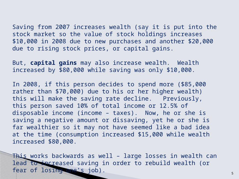
Saving from 2007 increases wealth (say it is put into the stock market so the value of stock holdings increases $10,000 in 2008 due to new purchases and another $20,000 due to rising stock prices, or capital gains. But, capital gains may also increase wealth. Wealth increased by $80,000 while saving was only $10,000.

In 2008, if this person decides to spend more ($85,000 rather than $70,000) due to his or her higher wealth) this will make the saving rate decline. Previously, this person saved 10% of total income or 12.5% of disposable income (income – taxes). Now, he or she is saving a negative amount or dissaving, yet he or she is far wealthier so it may not have seemed like a bad idea at the time (consumption increased $15,000 while wealth increased $80,000.

This works backwards as well – large losses in wealth can lead to increased saving in order to rebuild wealth (or fear of losing one’s job).

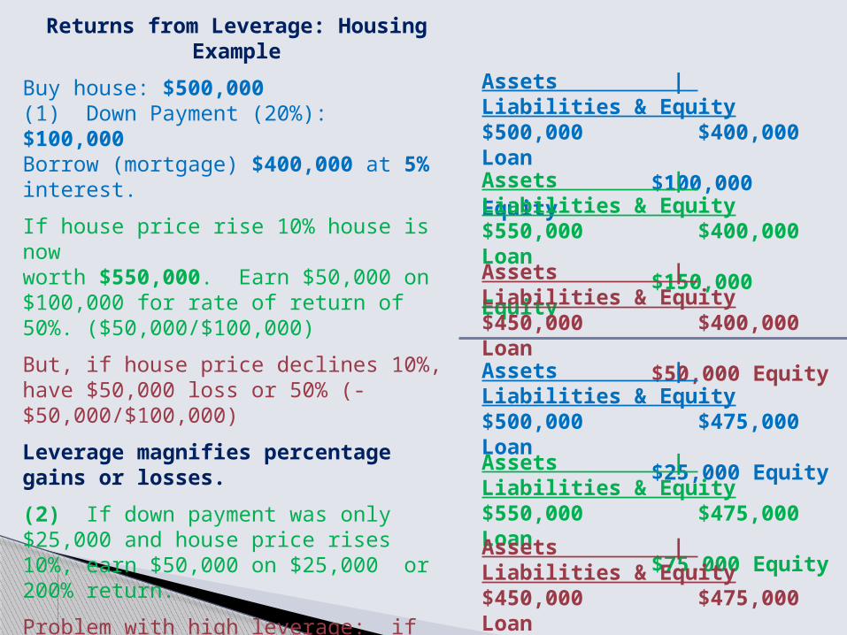
Returns from Leverage: Housing ExampleBuy house: $500,000 (1) Down Payment (20%): $100,000Borrow (mortgage) $400,000 at 5% interest.

If house price rise 10% house is nowworth $550,000. Earn $50,000 on $100,000 for rate of return of 50%. ($50,000/$100,000)

But, if house price declines 10%, have $50,000 loss or 50% (- $50,000/$100,000)

Leverage magnifies percentage gains or losses. (2) If down payment was only $25,000 and house price rises 10%, earn $50,000 on $25,000 or 200% return.

Problem with high leverage: if house price falls 5% or more (below $475,000), the homeowner will owe more than the house is worth – house is “underwater”. Housing prices fell 20-30% or more in many cases.

Assets | Liabilities & Equity$500,000 $400,000 Loan

$100,000 Equity

Assets | Liabilities & Equity$550,000 $400,000 Loan

$150,000 Equity

Assets | Liabilities & Equity$450,000 $400,000 Loan

$50,000 Equity

Assets | Liabilities & Equity$500,000 $475,000 Loan

$25,000 Equity

Assets | Liabilities & Equity$550,000 $475,000 Loan

$75,000 EquityAssets | Liabilities & Equity$450,000 $475,000 Loan

- $25,000 Equity

7

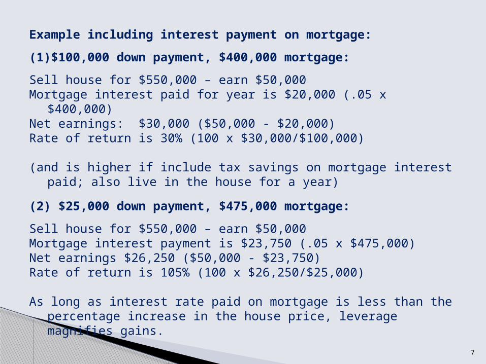
Example including interest payment on mortgage:

(1) $100,000 down payment, $400,000 mortgage:

Sell house for $550,000 – earn $50,000Mortgage interest paid for year is $20,000 (.05 x $400,000)Net earnings: $30,000 ($50,000 - $20,000)Rate of return is 30% (100 x $30,000/$100,000)

(and is higher if include tax savings on mortgage interest paid; also live in the house for a year)

(2) $25,000 down payment, $475,000 mortgage:

Sell house for $550,000 – earn $50,000Mortgage interest payment is $23,750 (.05 x $475,000)Net earnings $26,250 ($50,000 - $23,750)Rate of return is 105% (100 x $26,250/$25,000)

As long as interest rate paid on mortgage is less than the percentage increase in the house price, leverage magnifies gains.

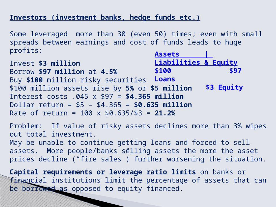
Investors (investment banks, hedge funds etc.)

Some leveraged more than 30 (even 50) times; even with small spreads between earnings and cost of funds leads to huge profits:

Invest $3 million Borrow $97 million at 4.5%Buy $100 million risky securities$100 million assets rise by 5% or $5 millionInterest costs .045 x $97 = $4.365 million Dollar return = $5 – $4.365 = $0.635 millionRate of return = 100 x $0.635/$3 = 21.2%

Problem: If value of risky assets declines more than 3% wipes out total investment.May be unable to continue getting loans and forced to sell assets. More people/banks selling assets the more the asset prices decline (“fire sales”) further worsening the situation.

Capital requirements or leverage ratio limits on banks or financial institutions limit the percentage of assets that can be borrowed as opposed to equity financed.

Assets | Liabilities & Equity$100 $97 Loans

$3 Equity

9

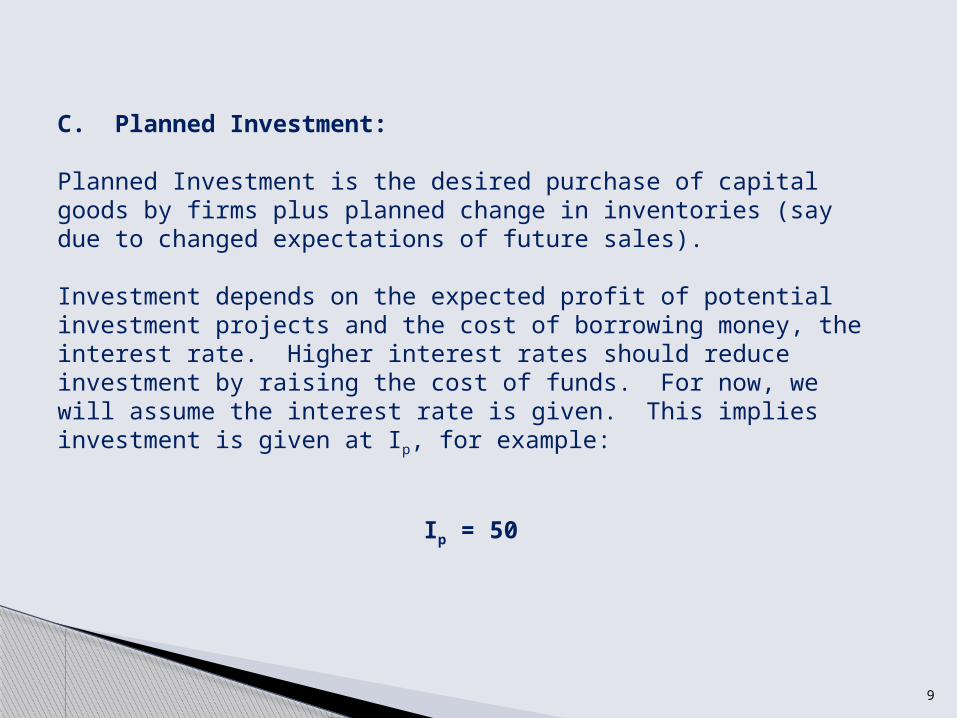
C. Planned Investment: Planned Investment is the desired purchase of capital goods by firms plus planned change in inventories (say due to changed expectations of future sales).  Investment depends on the expected profit of potential investment projects and the cost of borrowing money, the interest rate. Higher interest rates should reduce investment by raising the cost of funds. For now, we will assume the interest rate is given. This implies investment is given at Ip, for example:  

Ip = 50 

10

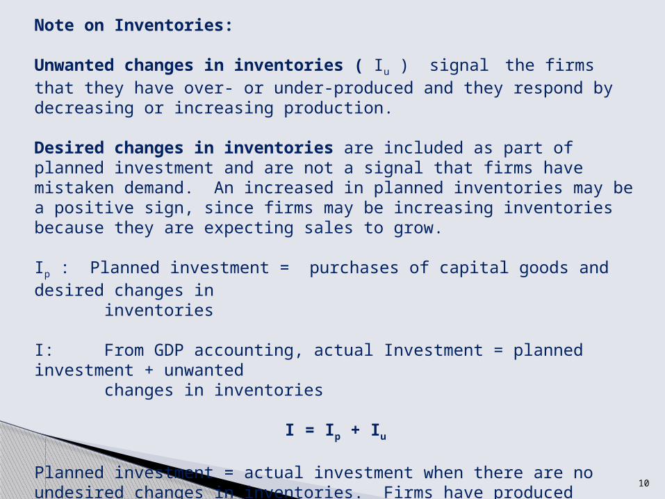
Note on Inventories:

Unwanted changes in inventories ( Iu ) signal the firms that they have over- or under-produced and they respond by decreasing or increasing production.  Desired changes in inventories are included as part of planned investment and are not a signal that firms have mistaken demand. An increased in planned inventories may be a positive sign, since firms may be increasing inventories because they are expecting sales to grow. Ip : Planned investment = purchases of capital goods and desired changes in inventories I: From GDP accounting, actual Investment = planned investment + unwanted changes in inventories 

I = Ip + Iu

 Planned investment = actual investment when there are no undesired changes in inventories. Firms have produced exactly what is demanded so there is no reason for them to increase or decrease production

11

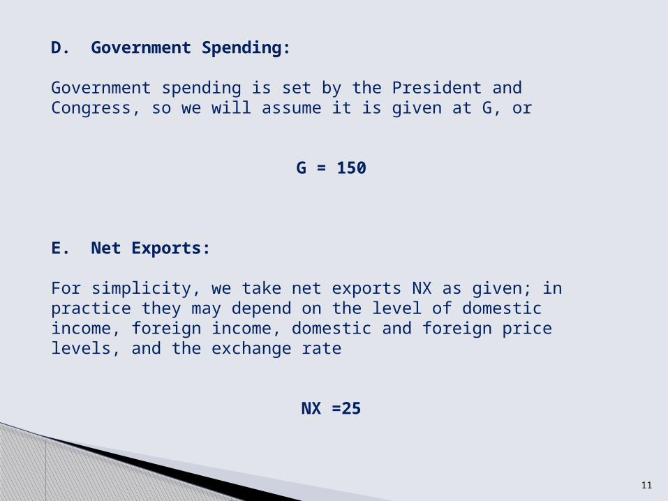
D. Government Spending: Government spending is set by the President and Congress, so we will assume it is given at G, or  

G = 150   E. Net Exports: For simplicity, we take net exports NX as given; in practice they may depend on the level of domestic income, foreign income, domestic and foreign price levels, and the exchange rate  

NX =25 

12

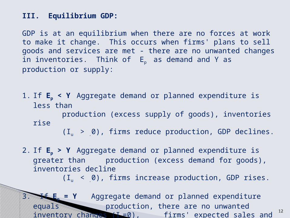
III. Equilibrium GDP: GDP is at an equilibrium when there are no forces at work to make it change. This occurs when firms' plans to sell goods and services are met - there are no unwanted changes in inventories. Think of Ep as demand and Y as production or supply:  1. If Ep < Y Aggregate demand or planned expenditure is less than

production (excess supply of goods), inventories rise (Iu > .0), firms reduce production, GDP declines.

 2. If Ep > Y Aggregate demand or planned expenditure is greater than

production (excess demand for goods), inventories decline (Iu < .0), firms increase production, GDP rises.

 3. If Ep = Y Aggregate demand or planned expenditure equals

production, there are no unwanted inventory changes (Iu=0), firms' expected sales and planned investment are met (I = Ip), there is no reason for them to change production. GDP is constant. This is the equilibrium GDP.

13

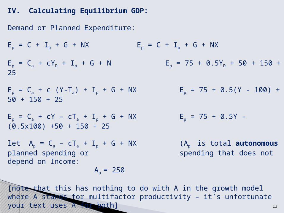
IV. Calculating Equilibrium GDP: Demand or Planned Expenditure: Ep = C + Ip + G + NX Ep = C + Ip + G + NX Ep = Ca + cYD + Ip + G + N Ep = 75 + 0.5YD + 50 + 150 + 25 Ep = Ca + c (Y-Ta) + Ip + G + NX Ep = 75 + 0.5(Y - 100) + 50 + 150 + 25 Ep = Ca + cY – cTa + Ip + G + NX Ep = 75 + 0.5Y - (0.5x100) +50 + 150 + 25 let Ap = Ca – cTa + Ip + G + NX (Ap is total autonomous planned spending or

spending that does not depend on Income:

Ap = 250

[note that this has nothing to do with A in the growth model where A stands for multifactor productivity – it’s unfortunate your text uses A for both] Ep = Ap + cY Ep = 250 + 0.5Y 

This is the equation of the planned expenditure curve . The intercept is Ap = 250 and the slope is c = 0.5.

14

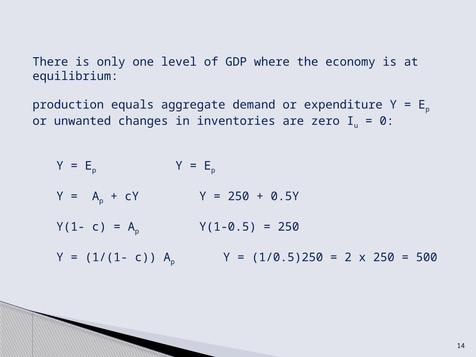
There is only one level of GDP where the economy is at equilibrium:  production equals aggregate demand or expenditure Y = Ep or unwanted changes in inventories are zero Iu = 0:  

Y = Ep Y = Ep

 Y = Ap + cY Y = 250 + 0.5Y

Y(1- c) = Ap Y(1-0.5) = 250 

Y = (1/(1- c)) Ap Y = (1/0.5)250 = 2 x 250 = 500

15

Y 2 Y 45 0

Y 3 Y 1

Ep

2

3 1

500 Equilibrium

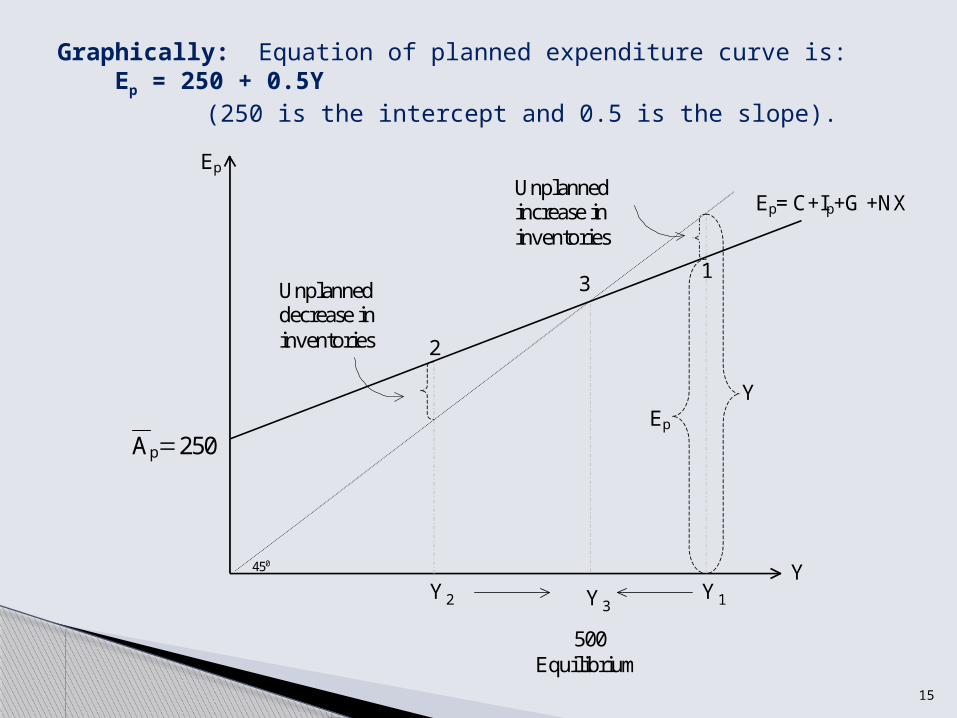
Unplanned decrease in inventories

Ep= C+Ip+G +NX

Y Ep

250 Ap

Unplanned increase in inventories

Graphically: Equation of planned expenditure curve is: Ep = 250 + 0.5Y (250 is the intercept and 0.5 is the slope).

16

Explanation of the 45 degree line: Equation of 45 degree line: Ep = Y (intercept is zero and slope is one)whatever is measured on the vertical axis equals what is measured on the horizontal axis (e.g. points (0,0), (100,100), (200,200), etc.). Here, the point where the Ep curve crosses the 45 degree line is where Ep = Y or it is equilibrium GDP.

17

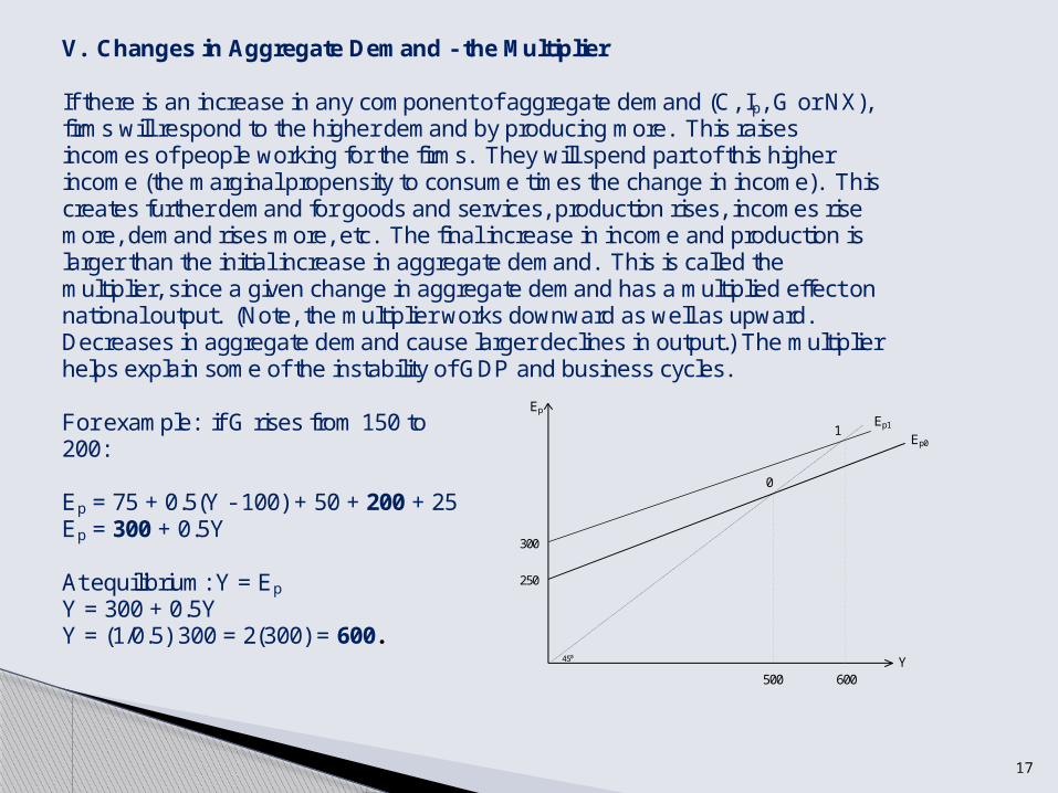
V. Changes in Aggregate Demand - the Multiplier If there is an increase in any component of aggregate demand (C, Ip, G or NX), firms will respond to the higher demand by producing more. This raises incomes of people working for the firms. They will spend part of this higher income (the marginal propensity to consume times the change in income). This creates further demand for goods and services, production rises, incomes rise more, demand rises more, etc. The final increase in income and production is larger than the initial increase in aggregate demand. This is called the multiplier, since a given change in aggregate demand has a multiplied effect on national output. (Note, the multiplier works downward as well as upward. Decreases in aggregate demand cause larger declines in output.) The multiplier helps explain some of the instability of GDP and business cycles. For example: if G rises from 150 to 200: Ep = 75 + 0.5(Y - 100) + 50 + 200 + 25 Ep = 300 + 0.5Y At equilibrium: Y = Ep Y = 300 + 0.5Y Y = (1/0.5) 300 = 2(300) = 600.

Ep0 Ep1 1

250

300

Y 45 0

Ep

0

500 600

18

The multiplier is the change in GDP for each $1 change in government spending:Y/ G GDP increased from $500 to $600 for a change of $100.Government spending rose from $150 to $200 for a change of $50.

Therefore, the multiplier is $100/$50 = 2. The coefficient on Ap in the equilibrium equation above is the multiplier: 1/(1- c). This is because a $1 increase in Ap will cause GDP to increase by 1/(1- c). If c = 0.5 as in our example above, the multiplier is 1/(1-0.5) = 1/0.5 = 2. This means that a $1 increase in Ap will cause a $2 increase in equilibrium GDP. The larger the marginal propensity to consume, the larger the multiplier, because if people spend more when their incomes rise, aggregate demand will rise more and so will production. Since the marginal propensity to save s = (1-c), the multiplier is also 1/s) Note: the multiplier for changes in taxes is smaller than that for other components of autonomous spending, such as G, because people do not spend every dollar of tax cuts, some is saved. They spend the marginal propensity to consume times the tax change. This implies that the tax multiplier is the marginal propensity to consume times the government multiplier: - c (1/(1-c). Expenditures rise less for a tax cut than for an increase in government spending, so GDP rises less.

19

VI. Taxes Proportional to Income: T = tY A more realistic model takes taxes to be proportional to income: T = tY (where T is dollar tax revenues and t is the tax rate) for example: T = 0.2Y General Case: Numerical Example:C = Ca + cYD C = 75 + 0.5YD

YD = Y - T = Y - tY YD= Y - 0.2YIp, G, NX given Ip = 50 G = 150 NX = 25 Aggregate demand or planned expenditure is: Ep = C + Ip + G + NX

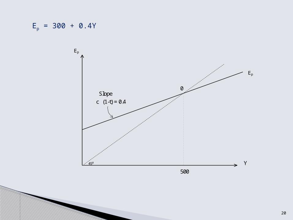
Ep = Ca + c(Y - tY) + Ip + G + NX Ep = 75 + 0.5(Y - 0.2Y) + 50 + 150 + 25 Ep = Ca + c(1-t)Y + Ip + G + + NX  equation of Ep curve, where autonomous spending Ap = Ca + Ip + G + NX: Ep = Ap + c(1-t)Y Ep = 300 + 0.4Y

Graphically (intercept of Ep is Ap = 300 and slope is c(1-t) = 0.4). The slope is smaller because when households get $1 more income, they pay $0.20 as taxes, disposable income is up $0.80 and they spend 0.5 (= mpc) of that or 0.4.

20

Y 45 0

Ep

Slope

c (1-t) = 0.4

Ep

0

500

Ep = 300 + 0.4Y

21

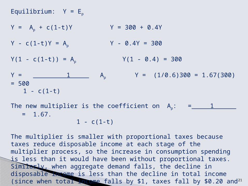
Equilibrium: Y = Ep

 Y = Ap + c(1-t)Y Y = 300 + 0.4Y Y - c(1-t)Y = Ap Y - 0.4Y = 300 Y(1 - c(1-t)) = Ap Y(1 - 0.4) = 300 Y = 1 Ap Y = (1/0.6)300 = 1.67(300) = 500

1 - c(1-t) The new multiplier is the coefficient on Ap: = 1 = 1.67.

1 - c(1-t) The multiplier is smaller with proportional taxes because taxes reduce disposable income at each stage of the multiplier process, so the increase in consumption spending is less than it would have been without proportional taxes. Similarly, when aggregate demand falls, the decline in disposable income is less than the decline in total income (since when total income falls by $1, taxes fall by $0.20 and disposable income declines $.80). Consumption declines less, so the multiplier is smaller.

22

Taxes act as an automatic stabilizer – when GDP declines, the decline in tax collections reduces the decline in expenditure so GDP falls less than it would otherwise; when GDP rises, the increase in taxes reduces the increase in expenditure so GDP rises less than it would otherwise.  A change in the tax rate will change the slope of the aggregate demand curve. The slope is c(1 - t). Therefore, an increase in the tax rate will make the slope flatter and reduce the equilibrium level of GDP. A higher tax rate will also reduce the multiplier because people will have less disposable income to spend at each stage of the multiplier process.  The Keynesian model can be made more and more complex by including other variables in the equations. For example, the consumption function may depend on interest rates and wealth, the investment demand may depend on interest rates and expected sales (proxied by GDP growth), and net exports may be affected by domestic income, foreign income, prices and the exchange rate. In addition, we may distinguish between different types of consumption (non-durables, durables or services) and different types of investment (plant and equipment or residential) and have a separate equation for each one. The basic structures of the models are the same but the equations are more complicated. Some macro models have more than 200 equations.

23

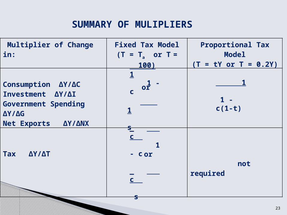
SUMMARY OF MULIPLIERS

Multiplier of Change in: Fixed Tax Model(T = Ta or T = 100)

Proportional Tax Model(T = tY or T = 0.2Y)

Consumption ∆Y/∆CInvestment ∆Y/∆IGovernment Spending ∆Y/∆GNet Exports ∆Y/∆NX

Tax ∆Y/∆T not required

1 1 - c(1-t)

1 1 - c

_ c s

1 s

_ c 1 - c

or

or