The Multinational Return Premium: Investor’s Perspective

Yeejin Jang*

Xue Wang

Xiaoyan Zhang

Abstract

Using monthly returns of 18,996 U.S. stocks over 1973-2015 and 23,965 stocks in 22 countries over 1990-2015, we find that multinational companies earn significantly higher returns than domestic companies by 23bps per month. We further investigate whether the return difference is driven by risk or known asset pricing anomalies, and find that none of them can fully explain the return premium of multinationals. The magnitude of the multinational return premium depends on the location of foreign operations. The return premium is more prominent for multinationals operating in countries where higher costs are incurred - countries with lower GDP growth, lower private credit, lower R&D export, higher labor cost, and larger geographic distance.

Keywords: multinational companies, international diversification, returns

JEL Classification: G11, G12, G15

____________________________

* We thank seminar participants at Purdue University, 2016 CICF, and 2016 SIF for helpful comments. All authors are affiliated with Krannert School of Management, Purdue University. Correspondence should be directed to Yeejin Jang, email: jang67@purdue.edu.

The Multinational Return Premium: Investor’s Perspective

Abstract

Using monthly returns of 18,996 U.S. stocks over 1973-2015 and 23,965 stocks in 22 countries over 1990-2015, we find that multinational companies earn significantly higher returns than domestic companies by 23bps per month. We further investigate whether the return difference is driven by risk or known asset pricing anomalies, and find that none of them can fully explain the return premium of multinationals. The magnitude of the multinational return premium depends on the location of foreign operations. The return premium is more prominent for multinationals operating in countries where higher costs are incurred - countries with lower GDP growth, lower private credit, lower R&D export, higher labor cost, and larger geographic distance.

Keywords: multinational companies, international diversification, returns

JEL Classification: G11, G12, G15

1

Introduction

The past few decades have witnessed the globalization of markets and the dramatic

growth in international business activities. In the U.S., between 1973 and 2015, the fraction of

public firms with foreign operations increased from 21% to 52%. From the firm’s perspective,

whether to expand operations internationally or to remain domestic is an important decision

because the geographical structure of a firm necessarily affects its future cash flows and risk

exposures. On the other hand, investors, who provide capital to the firm, focus more on the

returns of their investments in the firm.

Although many international business and strategy studies have tried to understand why

and how firms expand their operations abroad, there is only limited evidence on how the

international activities of firms affect stock returns, which investors care about the most. In this

paper, we fill this gap by asking the following questions from the perspective of investors: do

multinational companies have higher or lower returns than domestic companies, and therefore

are multinational companies more or less attractive to investors? If stock return differences exist

between multinationals and domestic firms, how is the geographic choice for foreign operations

related to the magnitude of the return differences? Following Pinkowitz, Stulz and Williamson

(2012), we define multinational companies (hereafter MNCs) as firms with significant operations

outside their home countries, and domestic companies (hereafter DCs) as firms with most of

their operations concentrated in domestic markets.

Based on previous literature, we establish a set of hypotheses on how the returns of

MNCs and DCs would differ.1 The first set of studies predicts that MNCs would earn lower

returns than DCs — the “MNC return discount” hypothesis. MNCs are better able to access

capital (Reeb et al. 2001), have a higher proportion of intangible assets (Morck and Young 1992),

and operate in more concentrated industries than DCs (Antras and Yeaple 2013). These distinct

characteristics of MNCs that motivate firms to have foreign operations are known to be

associated with lower stock returns. In addition, in imperfectly integrated global capital markets,

investors can diversify their portfolios internationally by holding MNCs, enhancing the stock

price of MNCs (Errunza and Senbet 1981, 1984). Therefore, MNCs are traded at higher prices

compared to DCs and hence have lower returns.

1 We briefly discuss the hypotheses in the introduction and a detailed literature review follows in section I.

2

A second set of studies takes the opposite position and supports the “MNC return

premium” hypothesis that MNC returns would be higher than DC returns. The main argument is

that operations in foreign countries incur additional risks that DCs do not have to bear such as

currency risks (Jorion 1990) or entry costs (Fillat and Garetto 2015). Thus, MNCs should have

higher returns than DCs as a result of the higher risk exposures. Meanwhile, because of the

complicated corporate structure, investors might demand a premium for processing information

on MNCs’ operations (Cohen and Lou 2012). Finally, the MNC return premium could be related

to two empirical asset pricing anomalies: the idiosyncratic volatility and profitability puzzles. As

MNCs have lower idiosyncratic volatility (Ang et al. 2006) and higher profitability (Novy-Marx

2013), MNCs should have higher returns than DCs.

We further develop our hypotheses by relating the return difference between MNC and

DC to MNCs’ location structures. When firms consider whether to become multinational, they

jointly make a decision on where to locate foreign operations. Previous studies have argued that

the location choice of foreign operations is determined by the key motivation of the international

expansion. For instance, firms that exhaust growth opportunities in domestic markets are more

likely to find a new product market to utilize their superior products and skills. Therefore, those

firms would enter countries with high growth opportunities (Errunza and Senbet 1981). On the

other hand, firms with limited capital would prefer to enter financially developed countries to

obtain access to capital in foreign countries (Baker, Foley, and Wurgler 2009, Houston,

Itzkowitz, and Naranjo 2007, Jang 2016). Next, the tax avoidance motivation would incentivize

firms to locate operations in countries with low corporate income tax (Desai, Foley, and Hines

2006). In this paper, to better understand the underlying reasons behind why MNCs deliver a

return premium or discount, we exploit the differences in characteristics and market conditions

of host countries where MNCs operate in explaining the magnitude of the return difference.

We start by testing the hypothesis on the return difference between MNCs and DCs. We

first examine the U.S. sample over 1973-2015 and document a strong pattern that the monthly

returns of MNCs are significantly higher than those of DCs by 23bps per month, after controlling

for size, value, momentum, and betas on Fama-French three factors and a foreign exchange rate

factor. The MNC return premium is robust across firm size groups, different time periods, and

most industries using both cross-sectional and time-series tests. When we extend our sample to

23,965 stocks in 22 developed countries over 1990-2015, the same pattern persists.

3

Why would MNCs have higher returns than DCs? We first identify alternative channels

that could possibly explain the return difference between MNCs and DCs. We consider the

following candidates: foreign exchange risk exposures, idiosyncratic volatility, skewness, default

risk, profitability, asset growth, industrial diversification, industry concentration, and foreign

institutional ownership. After controlling for each of the preceding return determinants, however,

the MNC return premium remains large and significant. We find that idiosyncratic volatility,

idiosyncratic skewness, gross profitability and asset growth significantly interact with the

magnitude of the MNC return premium, but neither diminishes the significance of MNC return

premium.

We next link the MNC return premium to the location choice of foreign operations.

Using a comprehensive dataset on MNCs’ country-level foreign sales, we examine the relation

between the return premium and host country characteristics such as GDP growth, labor cost,

financial market development, and corporate tax rate. We find that the higher operational costs

MNCs tend to pay in foreign countries, the higher the MNC return premium is. Specifically, the

MNC return premium is more prominent for MNCs operating in countries with lower GDP

growth, lower private credit, and lower R&D export. Using a global sample, we additionally find

evidence that MNCs have a higher premium if they operate in countries with higher labor costs

and in geographically more distant countries. These results imply that the MNC premium exists

to compensate for higher uncertainty in performance when MNCs enter the countries with higher

costs of foreign business.

Our paper relates to the international corporate diversification literature which focuses on

the valuation effect of corporate international diversification from a corporation’s perspective.

Previous studies evaluate the costs and benefits of international corporate diversification and

discuss what the optimal corporate structure is to maximize firm value. The usual empirical

approach is to compare the Tobin’s Q of a multinational firm to that of a portfolio of comparable

domestic firms operating in the same foreign countries as each foreign segment of the MNC. For

example, Denis, Denis and Yost (2002) and Fauver, Houston, and Naranjo (2004) show that

firms’ international diversification decisions are associated with lower Qs, or the so-called

4

“international diversification discount.”2 The Tobin’s Q measure is reasonable to test whether

having geographically diversified segments within a firm creates or diminishes the overall firm

value, but it is not an adequate measure for the purposes of our paper.

Our study focuses on the difference in stock returns between MNCs and DCs, rather than

Tobin’s Q, because a typical investor, presumably an outsider of the firm, would care more about

the stock returns. In addition, investors would directly compare returns of individual MNC and

DC stocks, because trading a portfolio of domestic firms in multiple foreign countries that

mimics an individual MNC stock requires high transaction costs. In this paper, we take the

investor’s perspective and answer the following question: if everything else remains equal, and

the firm’s multinational status is publicly available information, should a typical investor invest

in a multinational firm or a domestic firm? Our results clearly show that MNCs exhibit higher

returns than DCs over the past 40 years not only in the U.S. but also in 22 developed countries.

We examine alternative explanations and confirm that none fully explains the magnitude of the

MNC return premium. Therefore, we make distinct and significant contributions to the literature

by documenting that the multinational status of the firm is relevant information for investors. In

addition, we conduct a thorough analysis on how the locations of the foreign operations affect

the MNC return premiums, which provides deeper insights on how the MNC return premiums

are generated.

One closely related work is Fillat and Garetto (2015), who propose a theoretical model

and provide brief empirical results on the return difference between MNCs and DCs. They focus

on the high entry cost to foreign countries as one of the explanations on why MNCs earn higher

returns than DCs. Our paper provides a more comprehensive examination of the return difference

observed between MNCs and DCs, based on previous studies on why and how firms expand

operations abroad. We also consider alternative explanations for MNC return premiums, and

confirm that a large portion of the MNC return premium cannot be fully explained after

controlling for various risk factors. Further, by using international data and MNCs’ foreign

location information, we document that the magnitude of the MNC premium depends on a

variety of host country characteristics that reflect the benefits and costs of foreign operations.

2 Actually, the evidence of corporate international diversification discount is not conclusive. Creal et al. (2014) find that MNCs are traded at a premium, rather than a discount, when using a different benchmark. Hund, Munk and Tice (2014) argue that the existence of the diversification discount depends on the benchmark and methodology.

5

The remainder of the paper is organized as follows. Section I provides a comprehensive

literature review on why MNCs and DCs might have different returns, and how the MNCs make

the location decisions. Section II describes our data sample and reports summary statistics.

Section III and IV present our main empirical results for the U.S, and the global sample,

respectively. Section V concludes.

I. Literature Review and Hypothesis

The theoretical and empirical evidence on the determinants of firms’ international

diversification decisions provides insights on how these factors can lead to return differences

between MNCs and DCs. In this section, we first review related studies and categorize them into

two hypotheses: one predicting a MNC return discount and the other predicting a MNC return

premium. Then we review the theories that explain the choice of MNC foreign locations.

A. MNC Return Discount

Corporate diversification studies argue that because multinational firms diversify their

operations “geographically”, MNCs have lower cash flow volatility than DCs, which results in

lower default risks and more positively skewed cash flow distributions. Therefore, a MNC has a

put option like feature especially during an economic downturn. The lower default risk of MNCs

implies lower returns compared to DCs. For example, Vassalou and Xing (2004) and Chava and

Purnanandam (2010) both find a positive cross-sectional relationship between stock returns and

default risks.

A company can gain financial advantages in both internal and external capital markets

from diversifying operations (see Stein (2003) for a review). MNCs can allocate capital across

different divisions through internal capital markets when one of the subsidiaries performs poorly.

In addition, a lower default probability increases overall debt capacity and lowers the cost of debt

in external capital markets, according to Reeb et al. (2001). Consequently, with better access to

internal and external capital markets, MNCs are less financially constrained than DCs. Lamont et

al. (2001) and Whited and Wu (2006) argue that the extent to which firms are financially

constrained is negatively priced in stock returns because financially constrained firms are more

subject to common shocks such as a credit crunch or liquidity shock. Therefore, we expect to

observe lower returns for MNCs, which are less financially constrained, compared to DCs.

6

Early studies in international economics document that the intensity of a firm’s

international activity is industry-specific. In particular, empirical evidence shows that MNCs are

in highly concentrated industries, whereas DCs are in competitive industries (e.g. Antràs and

Yeaple (2013)). Hou and Robinson (2006) argue that firms in concentrated industries earn lower

returns than firms in competitive industries, because higher entry barriers in concentrated

industries decrease the probability of default of existing firms in those industries. The different

industry characteristics between MNCs and DCs imply that MNCs mostly operating in

concentrated industries would be traded at a discount compared to DCs in competitive industries. The internalization theory says that firms have incentives to expand their operations

abroad when they have a substantial amount of proprietary assets such as R&D. As intangible

assets have public good features, firms can increase value by exploiting these assets in broader

markets. Consistently, Morck and Yeung (1992) find that the values of MNCs are positively

associated with firms’ spending on R&D and advertisements. From an asset pricing perspective,

it has been shown that the market does not promptly revise its pessimistic expectation for firms

with higher intangible assets such as R&D (e.g. Chan, Lakonishock, and Sougiannis (2001)).

Therefore, MNCs’ long-term investments in intangible assets would be associated with lower

returns relative to DCs.

Finally, foreign operations across different countries can affect the base of investors who

provide capital to the companies. Early studies, such as Errunza and Senbet (1981, 1984),

focusing on investors’ portfolio diversification choices, argue that investors can indirectly

diversify their portfolios internationally by adding a MNC stock instead of individual foreign

stocks. This argument assumes that capital markets are not perfectly integrated, and there are

frictions in terms of information asymmetry and transaction costs when purchasing foreign

stocks. In imperfect global capital markets, if marginal investors are domestic investors who

prefer MNCs, they would highly value MNCs. Thus, we expect lower returns for MNCs than for

DCs.

B. MNC Return Premium

The first rationale for MNCs having higher returns is the higher risk exposure of MNCs

from their foreign operations. For instance, given that MNCs generate cash flows in different

currencies, MNCs are more likely to be exposed to foreign exchange rate risks than DCs. As a

7

result, investors may require rewards for bearing exchange rate risks. Previous papers, such as

Jorion (1990) and Griffin and Stulz (2001), find consistent evidence that the exposure to

currency risks is priced in returns. Therefore, we expect MNCs to have higher foreign exchange

betas and thus higher returns. In addition to foreign currency risks, firms operating abroad may

also face political or cultural risks in foreign countries, which may result in higher operational

costs, as indicated in Adler and Dumas (1975) and Reeb, Kwok, and Baek (1998). A recent paper

by Fillat and Garetto (2015) develops a real option value model and explains that MNCs are

highly exposed to negative shocks in foreign markets, because they are reluctant to cease

overseas operations due to the significant amount of sunk costs that have already been incurred.

We expect these foreign operations to have higher levels of risk exposures. Accordingly, we also

anticipate that MNCs will negate higher returns compared to DCs.

The transaction cost theory in international economics emphasizes production efficiency

as a main motivation for foreign direct investment (Caves 1971, Dunning 1973, Vernon 1979,

Buckley 1988, and Kogut and Zander 1993). The argument is that cross-border expansion occurs

when a firm can attain lower costs or higher productivity by directly owning foreign operations

than by importing/exporting to foreign markets (Hennart 1982). Therefore, MNCs tend to be

more productive and efficient compared to DCs (Fishwick 1982). A recent paper by Novy-Marx

(2013) documents that profitable firms generate significantly higher returns than unprofitable

firms. In this sense, we expect that the higher profitability of MNCs could result in higher returns

compared to DCs.

As MNCs operate in various countries with different regulations and legal treatments,

they have more complex organizational structures than DCs. MNCs usually consolidate financial

statements of multiple foreign subsidiaries and only report aggregated business information.

Hence, any detailed accounting information on the subsidiary-level operations or on transfers of

resources across subsidiaries is not readily available to investors through public sources. Because

of this complexity, it might be difficult for investors to evaluate the future prospects of a

business or to incorporate industry-specific or country-specific news to stock prices. Therefore,

investors would require higher returns for holding MNC stocks to compensate for bearing the

information uncertainty or inefficiency of information dissemination, as documented in Zhang

(2006), Cohen and Lou (2012) and Huang (2015).

8

Lastly, home bias literature provides a prediction on how domestic investors treat MNCs

differently from DCs. Domestic investors prefer to invest disproportionately in domestic stocks

rather than diversifying their portfolios internationally, which is called the “home bias” puzzle

(French and Poterba 1991). On the other hand, foreign investors show a preference for

multinational stocks (Dahlquist and Robertsson 2001). Previous papers try to explain the home

bias puzzle based on an information story: home investors have superior access to information

about domestic firms and economic conditions for domestic markets. If domestic investors

determine the prices at the margin and if they have superior information about DCs compared to

MNCs, they are willing to hold DCs despite their low average returns. Therefore, we would

expect to see a higher return for MNCs.

C. Choice of MNC Locations

Previous studies have stated that the location choice of foreign operations is related to the

reasons why firms expand their operations abroad, which potentially would affect the returns of

MNCs. A firm’s decision to become a MNC is an equilibrium outcome of multiple factors, and

host country characteristics and market conditions. Ultimately, where MNCs choose to operate

provides us with relevant information on the benefits and costs of those foreign operations

(Hanson, Matoloni, and Slaughter 2001). We summarize previous theoretical arguments for the

motivation of firms’ decision to be multinational into five groups, and link each motivation to

MNC’s location decisions.

First, theories of industrial organization justify foreign direct investment in the context of

imperfect product and factor markets. With imperfect competition, MNCs can achieve a

competitive advantage relative to local firms by selling superior products or producing their

goods by providing capital, technology, or managerial skills and using cheap labor and natural

resources in foreign countries (see, for example, Errunza and Senbet (1981)). An implication of

imperfect product markets is that firms that exhaust growth opportunities in domestic markets

are more likely to internationally expand to find a new product market to utilize their superior

products and skills. Thus, those firms will tend to enter fast-growing countries. Similarly, if the

goal of foreign investment is to lower the input costs, we would expect firms to expand

operations to countries with lower labor costs.

9

Second, if financial markets are imperfectly integrated, firms enter foreign countries to

gain access to financing and thus to lower the cost of capital. By having assets in foreign

countries, MNCs are able to access to local financing through their foreign subsidiaries; thus,

they can lower their cost of capital by exploiting the variation in financial market conditions

across countries (Baker, Foley, and Wurgler 2009, Houston, Itzkowitz, and Naranjo 2007, Jang

2016). If the main motivation of foreign expansion is to obtain access to financing, MNCs would

prefer to enter financially developed countries.

Third, under the U.S. tax law, profits from foreign operations of multinational companies

are taxed at the foreign tax rates in countries in which the profits are generated, and they may

additionally incur U.S. tax liabilities when repatriated. Operating in tax havens or low-tax

jurisdictions provides opportunities for tax avoidance, especially for firms that face high tax

burdens in home country (Desai, Foley, and Hines 2006). Thus, MNCs prefer to establish

operations in tax havens or countries with low corporate taxes to reallocate taxable foreign

incomes.

Fourth, internalization theory posits that firms internalize markets for their intangible

assets by directly investing in foreign countries (Caves 1971, Dunning 1973). Intangible assets

such as technologies, patents, and managerial skills are difficult to exchange or trade at arm’s

length because they are mostly based on firm-specific proprietary information. Thus, firms that

intend to exploit their intangible assets outside home countries are more likely to enter countries

where their intangible assets can be actively traded.

Lastly, the location choice can be affected by country-specific costs that would be

incurred when a firm establishes foreign operations. Previous studies suggest that firms prefer to

expand to the countries that are more familiar in terms of culture and those with low information

asymmetry. Geographic distance is one of the critical factors in the location decisions as higher

geographic distance would increase information asymmetry and limit active transfer of

knowledge that is required to succeed in foreign investment. In addition, political risks cannot be

easily hedged away so that firms are more likely to choose countries with lower political risks.

It is clear that a firms’ location choice reflects the benefits and costs of foreign operations

and the main motivations for foreign investment. However, previous studies explained above do

not provide direct predictions on whether the location decisions would be positively or

negatively associated with MNC returns, which is thus an empirical question. In the next section,

10

we directly examine whether the above hypotheses on location choices are associated with the

magnitude of MNC returns.

II. U.S. Data

A. Multinational vs. Domestic

Our U.S. sample includes U.S. publicly traded firms listed on the New York Stock

Exchange, American Stock Exchange, and NASDAQ, excluding firms incorporated outside the

U.S. We include ordinary common shares only and exclude ADRs. The monthly return data are

obtained from CRSP and accounting data from Compustat. Our sample period begins in January

1973 and ends in December 2015. We apply the following filters to the data: firms are required

to have positive total assets and non-missing total income at the end of the previous fiscal-year

end; market value of equity is more than $1 million; book value of equity is positive; monthly

return is between -100% and 1,000%; and B/M ratio is not in the top or bottom 1% in the country.

Following Pinkowitz, Stulz and Williamson (2012), we classify firms into MNC and DC

based on foreign income and foreign income taxes reported in annual financial statements. The

SEC (SEC Regulation §210.4-08(h)) requires any U.S. public firms to disclose pre-tax income

and deferred taxes for domestic and foreign operations separately, if any of those measures for

non-U.S. operations exceed 5% of the consolidated total. We define a firm as a MNC in a given

fiscal year if it reports non-missing foreign income (Compustat item: PIFO) or foreign income

taxes (Compustat item: TXFO) in any of the previous three years.3 It is possible that firms even

with large scale foreign operations sometimes do not report foreign income, especially when they

earn relatively low or negative foreign income. By using the information from the previous three

years, we alleviate the concern that firms that have a large foreign presence but earn low foreign

income in a specific year could be defined as domestic.

Other studies use alternative ways of defining multinationals. For instance, Denis, Denis,

and Yost (2002) rely on foreign sales information obtained from the Compustat Geographic

Segment database to define internationally diversified firms. There are several advantages of

using foreign income information instead of foreign sales to identify multinationals. First, we

have a broader sample of MNCs as the threshold for reporting foreign income is much lower (5%)

3 Foreign income tax variable (TXFO) is available starting from fiscal year 1969, while the pre-tax foreign income (PIFO) variable becomes available from fiscal year 1984. We use foreign income tax information only to define a MNC prior to 1984, but use both variables after 1985.

11

than that for reporting foreign sales (10%). Second, foreign sales reported in the Compustat

Geographic Segment database include exports of goods, whereas foreign income takes into

account the income generated in foreign subsidiaries. Therefore, non-missing foreign income

confirms the physical presence of firms in foreign countries. Third, we can use the consistent

definitions both for the U.S. and for the global sample. Lastly, foreign income information is

available from the early 1970s, allowing us to use a much longer time-series period than when

using foreign sales.4

Figure 1 reports the distribution of MNCs and DCs for the U.S. sample. In Panel A, about

34% of the U.S. firms are defined as MNCs on average over the sample period. The proportion

of MNCs has gradually increased during the 1980s and 1990s, reaching 32% in 2000 and 52% in

2015. In Panel B, we observe that the number of MNCs increased from 637 in 1973 to 1,895 in

2015. On the other hand, the number of DCs gradually increased from 2,340 since 1973, peaked

at 5,064 in 1997, and decreased to 1,721 in 2015. In Panel C, we report the average market

capitalization of MNCs and DCs. As expected, MNCs are significantly larger than DCs: the

average market capitalization of MNCs is $3,177 million, whereas that of DCs is $825 million.

The difference in market capitalization has increased over time.

In Table 1 Panel A, we compare the differences in firm-level characteristics and risk

exposures between MNCs and DCs. We report the basic stock characteristics for the firm-month

sample in Table 1 A1. Not surprisingly, compared to DCs, MNCs have higher market values and

lower B/M ratios. These findings suggest that if size and value effects dominate, MNCs would

have lower returns than DCs. The previous 6-month return is computed by summing up the

monthly returns for the past six months, and the difference between MNCs and DCs is negligible.

Next, we present the summary statistics on factor loadings for both MNCs and DCs in

Table 1 A2. We first use the Fama-French 3 factor model to obtain loadings on the market, size

and value factors. All factors for the U.S. are obtained from the Kenneth R. French Data Library.

To estimate the factor loadings of each stock, we estimate a time-series regression in each month

using daily returns, which allows the loadings to be time-varying. We require at least 15

observations in each month for estimation. Compared to DCs, MNCs have significantly higher

factor loadings on the market factor but lower loadings on both size and value factors, possibly

4 We find that our main results are quantitatively similar alternative definitions for MNCs based on the percentage of foreign sales and the percentage of foreign income. In Appendix A3, we discuss the robustness of our results for different definitions of MNC.

12

because the MNCs tend to be larger firms with lower B/M ratios. To estimate the foreign

currency risk, we construct a foreign exchange factor (FX) using the return of the trade-weighted

U.S. dollar index (major currencies) from the Federal Reserve Bank of St. Louis. The loading on

FX is estimated from the regression of excess return on MKT and FX using daily returns. The

mean currency beta for DCs is 0.019, and the mean currency beta for MNCs is 0.008. The MNCs’

loadings on currency risk are significantly lower than those of the DCs, which is contrary to our

prior. Choi and Jiang (2009) provide a reasonable explanation for MNCs’ lower currency betas:

MNCs manage foreign exchange risks more actively and effectively than DCs, and therefore it is

not clear that MNCs would necessarily have higher currency betas.

Next, we collect information on a few other characteristics that are related to stock

returns. Following Ang et al. (2006), we compute idiosyncratic volatility as the annualized

volatility of the residuals from the regressions of daily excess returns using the Fama-French 3

factor model. We estimate expected idiosyncratic skewness as in Boyer, Mitton, and Vorkink

(2010). Default probability is computed according to Vassalou and Xing (2004). Following

Novy-Marx (2013), we define gross profit as revenues minus cost of goods sold scaled by total

assets. Following Cooper, Gulen, and Schill (2008), we define asset growth as the change in total

assets scaled by lagged total assets. These accounting variables are computed on an annual basis,

and we exclude observations at the top and bottom 1%. We also measure whether a firm is

industrially diversified using the Compustat industrial segment database. Industry diversification

is defined as one if a firm reports more than one industrial segment in a given fiscal year.

Following Hou and Robinson (2006), we calculate a sales-based Herfindahl index to measure

industry concentration, where we use three-digit SIC industry classifications. A higher value of

the Herfindahl index indicates that an industry is more concentrated and thus less competitive.

Finally, we calculate the percentage of foreign institutional holdings out of the total shares

outstanding (% Foreign Holding) using quarterly 13-F filings. The foreign institutional holding

data are available for a much shorter time-series window, which start in 2000 rather than 1973.

We provide descriptive statistics of the above characteristics for the firm-year sample in

Table 1 A3. MNCs are significantly different from DCs in multiple dimensions, and the

differences are statistically significant. Consistent with diversification effects, MNCs have

significantly lower idiosyncratic volatility, idiosyncratic skewness and default probability

relative to those of DCs. MNCs are on average more profitable: the average gross profit of

13

MNCs is about 40%, while the DCs’ gross profit is 29%. The average asset growth rate for DCs

is 16.1%, and the average growth rate for MNCs is 13.7%, indicating the DCs have higher asset

growth rate. MNCs are more likely to be industrially diversified than DCs. In addition, MNCs

tend to operate in more concentrated industries as measured by the Herfindahl index of industry-

level sales, whereas DCs operate in more competitive industries. Lastly, for the subsample of

firms with institutional ownership information available, we find that the percentage of foreign

institutional holdings is lower for DCs, which potentially reflects the home bias of investors.

Given the prominence of accounting multiples in the valuation literature, we report two

key accounting ratios in Table 1 A4: P/E ratios and P/CF ratios. The average P/E ratio of DCs is

14.04, while that of MNCs is 16.51, with a large and significant difference of 2.47. The pattern

of P/CF ratios is quite similar. Following the accounting literature, high valuation ratios, such as

P/E, lead to a lower future return, which implies that MNCs might have lower returns than DCs.

B. Locations of Foreign Operations

We obtain the data on foreign operations of MNCs from the Compustat Geographic

Segment database, which provides information on the geographic segment-level sales. 5

Compustat Segment data are primarily sourced from the SEC 10-K filings. Although firms are

required to separately report sales into each geographic segment in their financial statement, the

country by country categorization of the segments is not mandatory. For this reason, sometimes

firms report geographic segments at the regional level or they aggregate multiple countries as

one geographic segment. For those cases, we are not able to obtain detailed information on

foreign operations at the country level. To better match country-level characteristics to each

geographic segment, in this section, we restrict the sample to MNCs that report positive amount

of foreign sales at the country level. About 62% of MNCs in our U.S. sample are matched to the

Compustat geographic segment database, and around 34% of them are dropped because they do

not report foreign sales at the country level. We find that MNCs that do not report foreign sales

at the country level tend to be smaller and have lower B/M ratios, lower previous returns, and

higher market and size betas than MNCs that report county-level sales information. However, we

5 It might be ideal to use the information on the location of MNCs’ assets to identify where MNCs operate. Unfortunately, as sales and profits are the only items that are required to be reported at the geographic segment level, the asset variable is mostly missing in the Compustat geographic segment database. Thus, we rely on foreign segment sales information to identify the location of foreign operations.

14

do not find any significant difference in returns after controlling for basic stock variables and

betas. Thus, we believe that restricting our sample to the MNCs with country-level foreign sales

information would not significantly bias our results.

In Table 1 Panel B, we report the top 20 host countries from which MNCs have foreign

sales. For each host country in each year, we calculate the percentage MNCs that generate

positive sales from the host country and the percentage of foreign sales from the host county

(conditional on reporting positive sales from the host country). We then report the time-series

averages. Sales to Canada and U.K. account for more than 40% of foreign sales. Emerging

markets such as China, Mexico and Brazil also contribute a large proportion of foreign sales to

U.S. MNCs. The distribution of MNCs’ foreign sales across countries demonstrates a large

variation in terms of sources of foreign income even within MNCs.

We consider various country-level characteristics based on the five categories of foreign

expansion motivations explained in Section I.C. First, if firms expand to foreign countries to take

advantage of different product market factors, MNCs would prefer to enter countries with high

growth opportunities and cheap labor costs. We use GDP growth from World Bank to estimate

growth opportunity. To estimate the labor input cost, we use the average monthly labor costs per

employee adjusted for PPI in USD, which are sourced from OECD, International Labor

Organization, or various government agencies located through web search. Second, if the main

motivation of foreign investment is to achieve access to foreign capital, firms would expand to

countries with developed financial markets. We consider two country-level measures for the

financial development in stock and bank loan markets: the first is market capitalization of listed

domestic companies as the percentage of GDP, and the second is domestic credit to private

sectors as the percentage of GDP. Both are obtained from World Bank. Third, to estimate the tax

advantage of having foreign operations, we collect the data on the corporate tax rate of host

countries from various sources including OECD and Worldwide Tax Summaries from PwC.

Fourth, the internalization theory predicts that firms with high intangible assets would have

operations in foreign countries where those assets can be actively traded. To estimate the

intensity of trade in intangible assets, we use the proportion of high-technology exports out of

manufacturing exports, sourced from World Bank. Lastly, firms prefer to locate in foreign

countries with low operational costs. To estimate the country-specific costs for establishing

business, we consider geographic distance, trade openness defined as the maximum of exports

15

and imports of goods and services as the percentage of GDP between home and host countries,

and political stability. The political stability variable is obtained from Political Risk Services

International Country Risk Guide.

In Appendix Table A2, we report the summary statistics on the country characteristics

variables over 1997 to 2015. There is a large variation in the host country characteristics across

countries. For example, while China has the highest GDP growth of 9.47%, Italy has the lowest

GDP growth at 0.43%. For labor cost, India has the lowest labor cost at $140.87 per month, and

Switzerland has the highest at $5487.30 per month. In terms of corporate tax rate, it ranges

between Hong Kong (16.58%) and Japan (42%). Overall, the host country characteristic

variables show great cross-country variation and may reflect the different costs and benefits of

foreign operations in a specific country.

III. The U.S. Evidence

In this section, we examine whether MNCs and DCs deliver different stock returns using

a sample of U.S. stocks from 1973 to 2015. We report the main results in Section III.A. and

robustness checks in Section III.B. Results on foreign operation are discussed in Section III.C.

A. Main Results

To establish the link between the firm’s MNC status and returns, we rely on a Fama-

MacBeth (1973) regression approach. In each month, we estimate a cross-sectional regression of

monthly excess returns on a MNC dummy and a variety of firm characteristics and risk

properties as follows:

𝑟𝑟𝑖𝑖,𝑡𝑡 = 𝑎𝑎𝑡𝑡 + 𝑏𝑏𝑡𝑡𝑀𝑀𝑀𝑀𝑀𝑀𝑖𝑖,𝑡𝑡−1 + 𝑐𝑐𝑡𝑡′𝑐𝑐𝑐𝑐𝑐𝑐𝑐𝑐𝑟𝑟𝑐𝑐𝑐𝑐𝑐𝑐𝑖𝑖,𝑡𝑡−1 + 𝑢𝑢𝑖𝑖,𝑡𝑡 . (1)

The MNC dummy and control variables are lagged by a month or a year (depending on the data

frequency), meaning that all this information is available at the end of previous month. After we

estimate the coefficients, 𝑎𝑎𝑡𝑡 , 𝑏𝑏𝑡𝑡, 𝑐𝑐𝑡𝑡 for each month, we average the monthly time-series of the

coefficients over the entire sample period. We compute the time-series standard errors for the

coefficients with a Newey-West (1987) adjustment with 3 lags to take into account time-series

dependence. If there is no link between the firms’ status as a MNC and future returns, after

16

controlling for firm characteristics and risk properties, we expect that the coefficient on the MNC

dummy would not be statistically different from zero.

Table 2 presents our estimation results for equation (1). We report six regressions in

Panel A. For each regression, we report the coefficients and their t-statistics. At the bottom of the

table, we report the adjusted R squared and the average fraction of MNCs. For all regressions,

we include standard firm-level characteristics that might affect future returns, such as Ln(size),

B/M, and past 6-month return. We also include firm-level risk exposures, including market beta,

size beta, value beta, and currency risk beta.6 All regressions include industry fixed effects based

on the Fama-French 30 industry specifications.

Regression I is our baseline regression. The coefficient on the MNC dummy is 0.226,

with a highly significant t-statistic of 5.02. Our results suggest a MNC return premium: after we

control for firm-level characteristics and risk exposures, MNCs deliver significantly higher

returns than DCs by 0.23% per month or around 2.71% per year. In addition, we find a negative

coefficient on firm size and positive coefficients on B/M and the past 6-month return. Those

coefficients on the firm-level characteristics are all statistically significant, and the signs are

consistent with previous literature. Out of market, size, value, and currency betas, only the size

beta is significant with a negative sign.

To confirm that our results are robust to different definitions for MNCs, in Appendix

Table A3, we estimate the regressions with continuous variables indicating the magnitude of

foreign operations instead of the dummy variable for MNCs. We use the percentage of foreign

sales and the percentage of foreign income. The coefficients on the % of foreign sales and % of

foreign income are positive and statistically significant, suggesting that the MNC premium

increases in the importance of foreign operations. The more a firm relies on foreign operations,

the higher the return premium is.

From the summary statistics in Table 1, we know that MNCs are on average larger than

DCs in terms of total assets and market capitalization. To make sure that the results are robust

across different size groups, we re-estimate equation (1) for firms with different sizes to allow

greater flexibility along the size dimension in the Fama-MacBeth framework. We first sort stocks

into quintiles each month, based on the market capitalization in the previous month, with group 1

6 As an alternative specification, we also estimate the regressions including the momentum beta. With this specification, the magnitude of the MNC coefficient decreases slightly to 0.214.

17

being the smallest and group 5 being the largest. Then we re-estimate equation (1) within each

size group. In this way we allow all coefficients, including the coefficient on the MNC dummy,

to vary across different size groups.

For regressions II to VI for firms within each size quintile, the MNC dummy remains

positive and statistically significant for all size groups, indicating that the MNC return premium

is robust across size. Interestingly, the MNC premium is much larger for small and medium-size

firms than for large firms. For the smallest size quintile, the coefficient on the MNC dummy is

0.358 with a t-statistic of 3.65. The three medium size quintiles have slightly smaller MNC

dummy coefficients ranging from 0.205 to 0.206. For the largest 20% of firms, the coefficient on

the MNC dummy decreases to 0.115 with a t-statistic of 2.04.

The bottom of the table presents the distribution of MNCs among the five size quintiles.

For the smallest size group, about 16.28% of firms are MNCs, while for the largest size group,

about 56.34% of firms are MNCs. This is consistent with the summary statistic indicating that

large firms are more likely to be MNCs. Overall, we find a MNC return premium for all size

groups, and the effect is much larger for smaller firms. The analysis by size groups also confirms

that our results are not driven by a specific subset of large or small stocks.

B. Alternative Explanations and Robustness

B1. Asset Pricing Anomalies vs. MNC Return Premium

Given the large literature in asset pricing on various return anomalies, it is natural to ask

whether the MNC return premium is driven by well-known empirical patterns. In this section, we

consider eight previously-documented empirical anomalies that predict cross-sectional stock

returns.

To examine whether these anomalies can explain away the MNC return premium, for

each pattern/anomaly, we include the key variable of the anomaly in equation (1) as an additional

control. If the MNC return premium is driven by the anomalies, the additional control

presumably would absorb the return difference associated with the MNC status, and the MNC

dummy coefficient would become smaller and insignificant. These results are reported in Table 3

Panel A. In the first 8 regressions, we include asset pricing anomalies one by one, and we include

all of them in the last regression. The number of months included in the regressions changes

across different specifications due to the data availability of each control variable added.

18

From summary statistics in Table 1, we observe that MNCs have lower idiosyncratic

volatility, lower idiosyncratic skewness, lower default probability, higher profitability and higher

asset growth. The above five characteristics are directly linked to five well-known patterns in

asset pricing literature. Ang et al. (2006) document the idiosyncratic volatility effect that firms

with higher idiosyncratic volatility have lower returns. Boyer, Mitton, and Vorkink (2010) claim

that investors prefer “lottery-like” stocks, which might be overpriced. Therefore, the

idiosyncratic skewness effect implies that firms with positive skewness would have lower returns

in the future. Campbell, Hilscher and Szilagyi (2008) find that the default probability coefficient

is negatively related with stock return. A recent study by Novy-Marx (2013) finds that gross

profit is positively related to expected return, which is called the profitability puzzle. Finally,

Cooper, Gulen, and Schill (2008) find the asset growth anomaly, documenting that asset growth

is negatively associated with subsequent abnormal returns.

In regression I to V, we include the above five variables as an additional control one by one

to examine whether the MNC dummy would decrease in significance and/or magnitude. In the

benchmark regression in Table 2, the MNC dummy coefficient is 0.226 with a t-statistic of 5.02.

For regression I to V, the MNC dummy coefficient varies between 0.157 and 0.272, all with t-

statistics above 3.50. The results suggest that none of the five anomalies can explain away the

MNC return premium. Consistent with previous studies, the above five control variables are all

significant themselves with consistent signs. This indicates that the five previously known

anomalies found in the literature also exist in our sample.

Firms normally consider two alternative diversification strategies: geographical

diversification and industrial diversification. As in Denis et al (2002), these two diversification

strategies are not substitutes for each other, and they might have different impacts on stock

returns. Table 1 shows that internationally diversified firms tend to be industrially diversified at

the same time. This raises the possibility that MNCs earn higher returns than DCs because they

are industrially diversified. Meanwhile, as documented in Cohen and Lou (2012), the industry-

level diversification could be positively associated with future returns due to the complex firm

structures. In regression VI, we consider whether industry diversification affects the return

difference related to geographic diversification. The coefficient on the industry diversification is

insignificantly different from zero, which indicates that after controlling for other characteristics,

19

the industry diversification does not affect stock returns. The coefficient on the MNC dummy

remains at 0.211 with a t-statistic of 4.73.

Hou and Robinson (2006) find that firms in concentrated industries (i.e. less competitive

industries) exhibit a return discount. In Table 1, we observe that MNCs appear more frequently

in less competitive industries. In regression VII, the coefficient on the industry concentration

variable is negative but not significant. The lack of significance is because we include industry

dummies, which is highly correlated with the concentration index at the industry level.7 The

coefficient on the MNC dummy is still 0.226 with a t-statistic of 5.00.

Finally, we examine whether foreign institutional investor holdings lead to return

differences between MNCs and DCs. We include the percentage of foreign institutional holdings

out of the total number of shares outstanding to indirectly control for home bias.8 Notice that

data for foreign holdings are available for a much shorter period, restricting the sample to 186

months of observations. After controlling for foreign institutional investor holdings, the MNC

dummy coefficient becomes slightly smaller but still significant at 0.217 with a t-statistic of

2.38.9

In the last regression in Table 3 Panel A, we include all the control variables mentioned

above except the percentage of foreign institutional holding due to the short period of data

availability. With all seven additional controls, the MNC dummy coefficient is 0.156, which is

still 69% of the magnitude in the baseline regression, and the t-statistic is highly significant at

2.48. Out of the six controls, idiosyncratic volatility, default probability, and asset growth are

significant with signs in line with our expectations. By and large, we confirm that the MNC

return premium cannot be entirely explained by previously documented anomalies.10

7 When we estimate regression VII without industry dummies as an alternative specification, the coefficient on industry concentration becomes more negative (-0.362) and significant at 5% level. 8 From regressions not reported, when we examine the percentage of foreign institutional holdings out of total institutional holdings, the results are similar. 9 We also consider the real option value theory in Fillat and Garetto (2015). However, the theory is based on the sunk cost incurred associated with entering a foreign market, which is not directly observable. We use fixed costs at both firm and industry levels as a proxy for sunk cost, but the fixed cost variables fail to explain the MNC premium. 10When we include the MNC dummy and the other control variables in the same regression, it proves robustness rather than causality. To understand channels through which MNCs earn higher returns than DCs, we further examine the possible driving forces for the higher returns associated with MNCs in more depth by using a two-stage approach. To save space, results are reported Appendix Table A4. We find that none of the nine channels can explain more than half of the MNC return premiums.

20

B2. Sub-period Patterns

Is it possible that main results are driven by specific time-periods? To estimate the

magnitude of MNC return premiums by sub-period, we divide our sample period into four sub-

periods: 1973-1983, 1984-1993, 1994-2003 and 2004-2015. The results are presented in Panel B

of Table 3. For the four 10-year sub-periods, the coefficient for the MNC dummy starts at 0.115

for 1973-1983, increases to 0.211 for 1984-1993, peaks at 0.426 for 1994-2003, and drops to

0.173 for 2004-2015. All coefficients are statistically significant over all sub-periods except in

the last 12 years. In Figure 2, we plot the time-series coefficients on the MNC dummy over the

entire U.S. sample period. The coefficient on the MNC dummy stays mostly positive over 1973

to 2015. However, consistent with our results by sub-periods, we observe the worst performance

for the MNC premium during the recent financial crisis: the coefficient on the MNC dummy is

strongly negative.

To examine the reason for the lower premium in the most recent period, we separately

look at the financial crisis period between 2007Q3 and 2009Q1. Part of the drop in the MNC

return premium and the lower statistical significance over the last 12 years is due to the financial

crisis. During 2007Q3 and 2009Q1, the MNC dummy has a negative coefficient of -0.279, yet is

statistically insignificant, possibly due to the short and noisy sample period. If we exclude the

financial crisis periods, MNCs earn significantly higher returns by 0.250% than DCs during the

period of 2004-2015. We also separate our samples based on the NBER economic recession

periods. We find that the coefficient for MNC dummy in a non-recession period is at 0.279 with

a t-statistic of 6.25, while during NBER recession periods, the MNC dummy coefficient is

insignificantly different from zero.

Combining all results in Panel B, we observe a clear pattern that MNCs have higher

returns than DCs over the past 43 years except during the financial crisis period and NBER

recessions. The theoretical model in Fillat and Garreto (2015) indicates that MNCs have higher

exposures to downside market risks, and thus they should have higher returns. Our empirical

results suggest that MNCs have lower returns than DCs during a financial crisis, which is

consistent with their model. However, the higher market risk exposures of MNCs may not be the

ultimate reason for the high returns of MNCs, because we allow market betas to vary over time

within the Fama-MacBeth framework. After controlling for the increased market risk exposures

21

of MNCs during recessions, we still find that the MNCs return premium is positive and

significant.

B3. A Portfolio Approach

The MNC return premium documented in Table 2 implies that a firm’s multinational

status might be useful information for investors to form their investment portfolios. Does a

trading strategy of taking long positions on MNCs and short positions on DCs create abnormal

returns? To answer this question, we first construct MNC and DC portfolios based on their MNC

status in the past year. Next, we calculate the monthly value-weighted excess returns of each

portfolio, and then obtain the abnormal returns (alphas) from a time-series regression of portfolio

excess returns on Fama-French three factors (FF3) and a momentum factor (FF4).

We present the portfolio returns, alphas, and their differences in Table 3 Panel C. The

average monthly excess return for MNCs is 0.921%, while the excess return for DCs is 0.806%.

The difference is 0.115% with a t-statistic of 1.57. Using the Fama-French three factor model,

we find that the monthly alphas of the MNC and DC portfolios are 0.059% and -0.098%,

respectively. The difference in alphas between MNC and DC portfolios is 0.156%, which is

statistically significant with a t-statistic of 2.16. When we add the momentum factor, the

difference in alphas is very similar at 0.155% per month with a t-statistic of 2.09. This result

implies that a trading strategy that exploits information on firms’ multinational status generates

significant and positive abnormal returns, especially after controlling for risk factors.

In the right half-panel of Panel C of Table 3, we sort firms into size quintiles and

construct MNC and DC portfolios within each size quintile. For the smallest firms, the excess

return difference is 0.392%, and the alpha for the FF4 model is 0.545%, both of which are highly

significant. For the next three size groups, the return differences are all significant and positive,

but the magnitude of returns to the MNC portfolios gradually decreases in firm size. For the

largest size group, the excess return difference is 0.128%, positive but insignificant, while the

alphas from the FF3 and FF4 models are 0.156% and 0.152%, both positive and significant.11

11 In Appendix A5, we present the return difference between MNC and DC by various industries, and we find that MNC return premiums are more prominent for tradable industries than for non-tradable industries.

22

C. Locations of Foreign Operations

To examine whether and how the locations of MNCs’ foreign operations are related to

the magnitude of MNC’s return differences, we estimate the Fama-MacBeth regression as

follows:

𝑟𝑟𝑖𝑖,𝑡𝑡 = 𝑎𝑎𝑡𝑡 + 𝑏𝑏1𝑡𝑡𝑀𝑀𝑀𝑀𝑀𝑀𝑖𝑖,𝑡𝑡−1 + 𝑏𝑏2𝑡𝑡𝑀𝑀𝑀𝑀𝑀𝑀 × 𝐻𝐻𝑐𝑐𝑐𝑐𝑐𝑐 𝑀𝑀𝑐𝑐𝑢𝑢𝑐𝑐𝑐𝑐𝑟𝑟𝐶𝐶 𝐼𝐼𝑐𝑐𝐼𝐼𝐼𝐼𝑐𝑐𝑎𝑎𝑐𝑐𝑐𝑐𝑟𝑟 + 𝑐𝑐𝑡𝑡′𝑐𝑐𝑐𝑐𝑐𝑐𝑐𝑐𝑟𝑟𝑐𝑐𝑐𝑐𝑐𝑐𝑖𝑖,𝑡𝑡−1 + 𝑢𝑢𝑖𝑖,𝑡𝑡 (2)

In addition to the MNC dummy, we add the interaction terms between the MNC dummy and the

indicator of host-country characteristics. For example, in the case of GDP growth, each host

country is defined as high GDP growth country if its GDP growth is above the median among

the 70 host countries over the sample period. For each MNC, in a given year, High GDP Growth

is defined as one if the firm has more than 50% of foreign sales in high GDP growth countries.

Thus, High GDP Growth represents MNCs that have most of their foreign operations in

countries with high growth opportunities. 12 If a specific host country characteristic is an

important driver of the MNC premium, we expect the coefficient on the interaction term (𝑏𝑏2𝑡𝑡) to

be statistically significant.

The results are reported in Table 4. First of all, the coefficients on the MNC dummy itself

are positive and significant, which is consistent with our main results, and provide the baseline

for the interaction terms. When we look at the interaction terms with various host country

characteristics, we find that the magnitude of the MNC premium depends on some of the

location choice variables with statistical significance.

The first set of location choice variables is related to economic conditions and the cost of

inputs such as labor, which are included in regression I and II. In regression I, the interaction

term of the MNC dummy with High GDP Growth is -0.270 with t-stat of -2.10. The result

implies that if MNCs have operations mostly in low GDP growth countries, they have higher

returns than DCs by 0.293% per month. In regression II, the interaction between the MNC

dummy and the Low Labor Cost dummy is -0.168, but statistically insignificant. The MNCs that

have selected the location for their foreign operations based on lowering labor costs do not have

significantly different returns from other MNCs.

12 We use alternative cutoffs other than 50% for the foreign sales, and the results are quantitatively similar.

23

Second, we consider the financial development of host countries. In regression III, the

interaction term for the MNC dummy with the high market capitalization variable is statistically

insignificant. In regression IV, when we consider the bank capital development of host countries,

we find that the coefficient on the interaction term is -0.136 with a t-stat of -1.97. This result

implies that the MNC premium is 0.280% per month compared to a DC, on average, but the

magnitude of MNC premium decreases by 0.136% per month for the MNCs that mostly locate in

countries with high private credit.

If the main motivation of expanding foreign operations is to avoid high corporate taxes in

a home country, MNCs would locate foreign operations in low corporate tax countries. We find

that in regression V, the interaction term is negative but insignificant.

Based on the internalization theory, we consider the risks of trading intangible assets.

Firms with more intangible assets have a stronger incentive to invest in foreign countries,

especially in the countries that have active markets for their main assets. In regression VI, we

find that the interaction term with the MNC dummy and the indicator for firms operating in

countries with high R&D exports is -0.184, which is statistically significant. That is, when firms

locate their foreign operations in countries with higher R&D exports, the MNC return premiums

would be lower by 0.18% per month.

Lastly, we look at additional proxies for the costs of foreign operations: geographic

distance, trade openness, and political stability. Conditional on the decision to be multinational,

firms might prefer to enter countries with lower trade costs (i.e. lower geographic distance and

higher trade openness) and with lower political risks (i.e. high political stability). In regressions

VII to IX, we do not find the coefficients of interaction terms statistically significant.

Overall, by using the detailed data on the geographic structures of MNCs, we find that

the return premium becomes more prominent for MNCs operating in countries with lower GDP

growths, lower private credit, and lower R&D exports. These results suggest that MNC return

premium is higher if the foreign operations are located in countries with lower benefits of foreign

operations, and the high return is probably compensation for the high uncertainty related to

performance in these countries.

24

IV. The Global Evidence

Is the MNC premium U.S. specific or does it exist in other countries outside the U.S. as

well? To answer this question, we examine the return difference between MNCs and DCs in non-

U.S. countries. We introduce the data in Section IV.A. The main results for the global sample are

presented in Section IV.B. In Section IV.C, we investigate possible explanations for the MNC

return premium in the global sample.

A. Global Sample Data

For the global sample, we include 23 countries that are classified as developed markets

by MSCI as of December 2015, which includes Australia, Austria, Belgium, Canada, Denmark,

Finland, France, Germany, Hong Kong, Ireland, Israel, Italy, Japan, the Netherlands, New

Zealand, Norway, Portugal, Singapore, Spain, Sweden, Switzerland, United Kingdom, and the

U.S. For countries outside of U.S., we obtain U.S. dollar-denominated monthly stock returns

from Datastream and annual accounting data from Worldscope. We include ordinary common

stocks only and exclude depositary receipts (DRs), real estate investment trusts (REITs), and

preferred stocks.13 Our sample period begins in January 1990 and ends in December 2015. The

sample starts from 1990 because Worldscope data coverage on international firms is limited

before 1990 for several countries.14 As in the U.S. sample, we classify firms into MNCs and DCs

in the global sample based on the foreign income variable (Worldscope item: WC08741). A firm

is defined as a MNC if it reports non-missing foreign income in any of the previous three years.

Summary statistics on the global sample are reported in Table 5. In Panel A, we report

the average number of MNCs and DCs each year, as well as their average market capitalization

by country. The proportion of MNCs in other countries is much lower compared to the U.S.

sample. The proportion of MNCs varies considerably across countries (8.82% to 37.77%), and

MNCs are substantially larger in terms of market capitalization than DCs as in the U.S.

Specifically, firms in Hong Kong, Ireland, Singapore and U.K. are more globalized (more than

13 Following Karolyi and Wu (2012), we also exclude stocks with name including “REIT”, “REAL EST”, “GDR”, “PF”, “PREF”, “PRF”, “ADS”, “CERTIFICATES”, “RESPT”, “Rights”, “Paid in”, “UNIT”, “INCOME FD”, “INCOME FUND”, “HIGH INCOME”, “INC.&GROWTH”, “INC.&GW”, “UTS”, “RTS”, “CAP.SHS”, “SBVTG”, “STG.SAS”, “GW.FD”, “RTN.INC”, “VCT”, “ORTF”, “HI.YIELD”, “GUERNSEY”, “DUPLICATE”, “DUAL PURPOSES”, and “NOT Rank for Dividend”. 14 Here we list the countries which enter our sample after 1990: the Netherlands (1992), New Zealand (1992), Switzerland (1994), Germany (1996), Sweden (1996), Israel (1997), Norway (1997), Austria (2002), Denmark (2003), Belgium (2004), Finland (2005), Portugal (2005), Italy (2006), Spain (2006).

25

30% of firms are MNCs), while firms in Norway, Sweden, and Israel are more likely to focus on

domestic operations (less than 10% of firms are MNCs).

Panel B reports summary statistics on firm level characteristics and risk exposures. There

are two differences between the global sample and the U.S. sample. First, we construct a “global

accessibility” variable to measure the extent to which globalization of financial markets affects

the return difference between MNCs and DCs. As documented in Karolyi and Wu (2012),

globally accessible firms might have different risk properties than locally accessible firms, which

could drive the difference in returns between MNCs and DCs. We compute the global

accessibility dummy, which equals one if the firm is globally accessible and zero otherwise,

following Karolyi and Wu (2012).15

The second difference for the global sample is that we compute the betas differently. For

the U.S. analysis, we only consider the U.S. risk factor exposures by including betas on market,

size, and value factors measured in the U.S. market. In the global sample analysis, following

Bekaert, Hodrick and Zhang (2009), we include risk exposures to both local and global risk

factors to accommodate for all possible levels of integration in global financial markets. If the

global capital markets are fully integrated, then only the global factors are relevant. If the global

capital markets are fully segmented, then only the local factors are relevant. If they are partially

integrated, then we would expect both global and local factors to be relevant. Following Bekaert

et al. (2009), we consider the global-local Fama-French 3 factor model, where we control for

both global and local market, size, and value factors. We first calculate a country-level market

factor as the value-weighted return of all firms in that country. To obtain country-level size

factors, for each month we sort firms into three size groups within the country based on the 6-

month lagged market value, and then compute the value-weighted return difference between

firms in the bottom tercile (smallest) and firms in the top tercile (biggest). Similarly, we calculate

the country value factor as the value-weighted return difference between firms in the highest

B/M tercile and the lowest B/M tercile. The global factors are calculated as the value-weighted

15 A firm is defined as globally accessible if one of its securities is listed in any of the following markets: (i) U.S., including NYSE/AMEX, NASDAQ, and the Non-NASDAQ OTC markets; (ii) U.K., including the London Stock Exchange, London OTC Exchange, London Plus Market, and SEAQ International; (iii) Europe, including Euronext at Amsterdam, Brussels, Lisbon, Paris, and EASDAQ; (iv) Germany in which the Frankfurt Stock Exchange is located; (v) Luxembourg in which the Luxembourg Stock Exchange is located; (vi) Singapore, including the Singapore Stock Exchange, Singapore OTC Capital, and Singapore Catalist; and (vii) Hong Kong in which the Hong Kong Stock Exchange is located. Under this definition, all the firms in the U.S., Belgium, Portugal, and Singapore are globally accessible.

26

sum of country level factors, where the weight equals the lagged market value of all stocks in

each country. For the currency risk, we construct the same foreign exchange factor (FX), as with

the U.S. testing, using the return of the trade-weighted U.S. dollar index (major currencies) from

the Federal Reserve Bank of St. Louis. The loading on FX is estimated from the regression of

excess returns on the global market, local market and FX. The betas are estimated at the firm

level with time-series regressions in each month using daily returns, which allow the loadings to

be time-varying. For the global sample, idiosyncratic volatility is estimated from the regression

of daily excess return on the global and local market, size and value factors. We exclude

observations in the top and bottom 1% of factor loadings in each month to exclude outliers.

We report the summary statistics of our global sample in Panel B of Table 5. Similar to

the U.S. sample, we find that MNCs are larger, have lower B/M ratios and higher past returns

than DCs. MNCs also have lower idiosyncratic volatility, higher profitability, and lower asset

growth than DCs, and they are more globally accessible. In terms of betas, MNCs have higher

exposures to both global- and local-market risks and lower global- and local-size factors than

DCs while the exposures to value factors are mixed. For the currency betas, as opposed to the

U.S. sample, MNCs in non-U.S. countries have significantly higher currency betas than DCs.

We obtain locations of foreign operations of MNCs in the global sample from Capital IQ.

Capital IQ collects the data on sales by geographic segments of companies in major countries

from various sources, and the primary source is financial statements of firms, which are

equivalent to 10-Ks of U.S. firms. As for the U.S. sample, for an analysis of MNCs’ foreign

locations, we restrict our global sample to the MNCs that report at least one positive amount for

foreign sales at the country level. We consider nine country-level variables for host country

characteristics, similar to the U.S. analysis: GDP growth, labor cost, market capitalization,

private credit, corporate tax, R&D exports, geographic distance, trade openness, and political

stability.

In Table 5 Panel C, we report the top 20 host countries of our global sample. The list of

popular countries for non-U.S. MNCs is similar to that of U.S. MNCs. The U.S. is the top

country that hosts a number of foreign MNCs, followed by the U.K., Japan and Canada.

27

B. Main Results on the Global Sample

For the global sample, we re-estimate the benchmark equation (1) with both country fixed

effect and industry fixed effect. The industry classification is based on the FTSE level-4 industry

identifications and SIC, as in Bekaert, Hodrick and Zhang (2009).

Table 6 reports the Fama-MacBeth regression results for the global sample. To save

space, we present results for firms in all countries, U.S. only, and non-U.S. countries separately.

We use factor loadings from the global-local Fama-French three factor model. As before, we

control for firm characteristics such as B/M, Ln (size), past 6-month return, and global and local

factor loadings.

For all firms in the global sample in regression I, the MNC dummy coefficient is 0.237

with a t-statistic of 4.59. This suggests that in the global sample, MNCs have higher returns than

DCs by 0.237% per month, and the difference is highly significant. Compared to 0.259 in the

U.S. sample (regression II) over the same sample period, the magnitude of the MNC dummy

coefficient using the global sample is slightly smaller, but they are similarly significant. When

we move on to the non-U.S. sample in regression III, the coefficient on the MNC dummy

becomes 0.145 with a t-statistic of 2.85, which indicates that the MNC premium is also sizable

and significant in non-U.S. countries. For the control variables, size, BM, and past returns are all

significant with expected signs. For the betas, the size betas are significant but with negative

signs.

C. Alternative Explanations for the MNC Return Premium

For the global sample, due to data limitations, we are unable to conduct a thorough

robustness check as in the U.S. sample, but we focus on the idiosyncratic volatility, gross

profitability, asset growth, and global accessibility as additional controls. As before, if any of the

controls is the reason for the MNC premium, we expect that the MNC dummy would lose its

significance by controlling for these anomalies.

Results are presented in Table 7. In regressions I to IV, we include the idiosyncratic

volatility, profitability, asset growth and global accessibility variable one by one, and in

regression V, we include all four controls. The MNC dummy coefficient varies between 0.159

and 0.254, and is always statistically significant. Among the four controls, the coefficient on

idiosyncratic volatility is negative as expected, but it is statistically insignificant. The coefficient

28

on gross profit is positive and significant, and the coefficient on asset growth is negative and

significant, both of which are the same as in the U.S. sample. Finally, the coefficient on global

accessibility is 0.637 and statistically significant, indicating that access to the global capital

market is an important determinant of stock returns.

In column V, when we include all control variables, the MNC premium decreases to

0.159% per month, but it remains statistically significant with a t-statistic of 2.32. That is to say,

the MNC return premium is positive and significant in the global sample, and the magnitude of

the MNC premium cannot be explained by the idiosyncratic volatility, gross profit, asset growth

and global accessibility effects.

D. Locations of Foreign Operations

Parallel to the U.S. results, here we examine how the location of the foreign operation

affects the return premium associated with MNCs in the global sample. We re-estimate the

Fama-MacBeth regressions as in equation (2) with the global sample.

Instead of using the whole sample median to determine whether a country has high or

low GDP growth as in the U.S. analysis, with the global sample, we are able to compare the

relative country characteristics between home and host countries. For each country-level

characteristic except geographic distance, host countries are sorted into the high (low) group if

the value of the host country is above (below) the value of the home country. For geographic

distance, host countries are sorted into the high (low) group if the distance between the host and

home country is above (below) the median. For each MNC, high (low) host country

characteristic equals 1 if more than 50% of foreign sales come from host countries in the high

(low) group.16 In addition, the regressions for the global sample include country dummies.

The results are reported in Table 8. First of all, the coefficients on the MNC dummy itself

are all positive and significant, indicating the baseline MNC return premium is also positive and

significant.

For the economic condition variables in regression I and II, we find that the interaction

coefficient between the MNC dummy and high GDP growth is -0.264 with a t-statistic of -3.44.

That is to say, if a firm’s foreign operation is located in a country with lower GDP growth, the

MNC return premium is reduced by 0.26% per month, while the unconditional MNC return

16 We also estimate regressions using the same specifications for the U.S. sample, and the results are similar.

29

premium is 0.42% per month. Similarly, if a firm’s foreign operation is located in a country with

lower labor cost, the MNC return premium is reduced by 0.12% per month, and the coefficient is

marginally significant. The results are similar to those for the U.S. sample.

For the country financial development variables in regression III and IV, the interaction

coefficients on high market cap and high private credit are both negative and significant,

indicating that the MNC premium is more prominent for the MNCs operating in countries with

less financial development.

When we look at the corporate tax rate in regression V, the coefficient on the interaction

term is small and insignificant, which implies that tax considerations do not have a significant

impact on return differences. For intangibility of assets, we find in regression VI, the MNC

return premium would be significantly reduced if the foreign operation is located in countries

with higher R&D exports.

Finally, from the perspective of operational cost, the interaction between the MNC

dummy and low geographic distance is -0.159 and statistically significant. The MNC return

premium is more prominent if the foreign operations are distant from the home country.

To summarize, MNCs operating in foreign countries with lower GDP growth, higher

labor costs, lower financial development, and greater geographic distance are associated with a

higher MNC premium, consistent with the U.S. results.

V. Conclusions

Using the monthly returns of 18,996 individual U.S. stocks from 1973 to 2015, we find

strong evidence that multinational stocks earn significantly higher returns by 23bps over

domestic stocks. This MNC return premium is persistent for different size groups and over

different time periods, while the magnitude of the MNC premium is much stronger in smaller

firms and during non-recession times. The higher returns of MNCs are not associated with

previously known return determinants. We consider various determinants, including

idiosyncratic volatility, idiosyncratic skewness, default probability, profitability, asset growth,

industry diversification, industry concentration, and foreign investors’ holdings. After controlling

for these potential factors, we confirm the strong and reliable explanatory power of a firm’s

multinational status in stock returns.

30

Based on previous studies on the determinants of international corporate diversification

strategies, we also examines various alternative explanations by which MNCs yield higher

returns than DCs. Interestingly, foreign exchange risk does not seem to be an important channel

explaining a MNC’s higher returns. None of the existing risk factors or know anomalies can fully

explain the magnitude of MNC premium. We find a similar pattern of higher monthly stock

returns for MNCs compared to DCs when we use a sample of 23,965 stocks in 22 developed

countries over the period 1990-2015. The results using the global stock returns are robust to

various specifications controlling for both local- and global-factors.

The return premium is clearly associated with the location of MNC’s foreign operations.

We find that the MNC return premiums become more prominent for MNCs operating in

countries with lower GDP growth, lower private credit, and lower R&D exports. Overall, the

MNC return premium is higher if MNCs’ foreign operations are located in foreign countries with

lower benefits (higher costs). The analysis of MNC’s foreign operations suggests a potential

source for the MNC return premium: investors are compensated for the high uncertainty related

to firm performance in countries with high foreign operational costs through higher stock returns.

Our findings provide strong evidence that the existence of firms’ international activities is

relevant in determining stock returns. One implication of our results is that as firms’ operations

become more globalized, international expansion decisions would affect how investors recognize

those firms in the global stock markets. Therefore, understanding why and how firms expand

their operations abroad would provide insights on how investors incorporate that information

into stock prices.

31

References

Adler, Michael, and Bernard Dumas, 1975, Optimal international acquisitions, Journal of Finance 30, 1-19.

Antràs, Pol, and Stephen R Yeaple, 2013, Multinational firms and the structure of international trade (No. w18775). National Bureau of Economic Research.

Ang, Andrew, Robert J. Hodrick, Yuhang Xing, and Xiaoyan Zhang, 2006, The cross-section of volatility and expected returns, Journal of Finance 61, 259-299.

Ang, Andrew, Robert J. Hodrick, Yuhang Xing, and Xiaoyan Zhang, 2009, High idiosyncratic volatility and low returns: International and further US evidence, Journal of Financial Economics 91, 1-23.

Baker, M., Foley, C.F. and Wurgler, J., 2009. Multinationals as arbitrageurs: The effect of stock market valuations on foreign direct investment. Review of Financial Studies, 22(1), pp.337-369.

Bekaert, Geert, Robert J. Hodrick, and Xiaoyan Zhang, 2009, International stock return comovements, Journal of Finance 64, 2591-2626.

Boyer, Brian, Todd Mitton, and Keith Vorkink, 2010, Expected idiosyncratic skewness, Review of Financial Studies 23, 169–202.

Buckley, Peter J., 1988, The limits of explanation: Testing the internalization theory of the multinational enterprise, Journal of International Business Studies 19, 181-193.

Campbell, John Y., Jens Hilscher, and Jan Szilagyi, 2008, In search of distress risk, Journal of Finance 63, 2899-2939.

Caves, Richard E, 1971, International corporations: The industrial economics of foreign investment, Economica 38, 1-27.

Chan, Louis KC, Josef Lakonishok, and Theodore Sougiannis, 2001, The stock market valuation of research and development expenditures, Journal of Finance 56, 2431-2456.

Chava, Sudheer, and Amiyatosh Purnanandam, 2010, Is default risk negatively related to stock returns, Review of Financial Studies 23, 2523-2559.

Choi, Jongmoo Jay, and Cao Jiang, 2009, Does multinationality matter? Implications of operational hedging for the exchange risk exposure, Journal of Banking & Finance 33, 1973-1982.

Cohen, Lauren, and Dong Lou, 2012, Complicated firms, Journal of Financial Economics 104, 383-400.

Cooper, Michael J., Huseyin Gulen, and Michael J. Schill, 2008, Asset growth and the cross-section of stock returns, Journal of Finance 63, 1609-1651.

Creal, Drew D., Leslie A. Robinson, Jonathan L. Rogers, and Sarah L. C. Zechman, 2014, The multinational advantage, Working paper, University of Chicago.

32

Dahlquist, Magnus, and Göran Robertsson, 2001, Direct foreign ownership, institutional investors, and firm characteristics, Journal of Financial Economics 59.3, 413-440.

Denis, David J., Diane K. Denis, and Keven Yost, 2002, Global diversification, industrial diversification, and firm value, Journal of Finance 57, 1951-1979.

Desai, M.A., Foley, C.F. and Hines, J.R., 2004. Foreign direct investment in a world of multiple taxes. Journal of Public Economics, 88(12), pp.2727-2744.

Dunning, John H, 1973, The determinants of international production, Oxford Economic Papers 25, 289-336.

Errunza, Vihang R., and Lemma W. Senbet, 1981, The effects of international operations on the market value of the firm: Theory and evidence, Journal of Finance 36, 401-417.

Errunza, Vihang R., and Lemma W. Senbet, 1984, International corporate diversification, market valuation, and size-adjusted evidence, Journal of Finance 39, 727-743.

Fama, Eugene F., and James D. MacBeth, 1973, Risk, return, and equilibrium: Empirical tests. The Journal of Political Economy, 607-636.

Fauver, Larry, Joel F. Houston, and Andy Naranjo, 2004, Cross-country evidence on the value of corporate industrial and international diversification, Journal of Corporate Finance 10, 729-752.

Fillat, José L., and Stefania Garetto, 2015, Risk, returns, and multinational production, The Quarterly Journal of Economics, forthcoming.

Fishwick, Frank, 1982, Multinational companies and economic concentration in Europe (Gower).

French, Kenneth R., and James M. Poterba, 1991, Investor diversification and international equity markets, American Economic Review 81, 222-26.

Griffin, John M., and René M. Stulz, 2001, International competition and exchange rate shocks: a cross-country industry analysis of stock returns, Review of Financial Studies 14, 215-241.

Hanson, G.H., Mataloni Jr, R.J. and Slaughter, M.J., 2001. Expansion strategies of US multinational firms (No. w8433). National bureau of economic research.

Hennart, Jean-Francois, 1982, A theory of multinational enterprise (University of Michigan Press).

Hou, Kewei, and David T. Robinson, 2006, Industry concentration and average stock returns, Journal of Finance 61, 1927-1956.

Houston, J.F., Itzkowitz, J. and Naranjo, A., 2007. Borrowing beyond borders: The geography and pricing of syndicated bank loans. Available at SSRN 969735.

Huang, Xiang, 2015 Thinking Outside the Borders: Investors’ Underreaction to Foreign Operations Information, Review of Financial Studies 28, 3109-3152.

Hund, John, Donald Monk, and Sheri Tice, 2014, Manufactured diversification discount, Working paper, Rice University.

33

Jang, Yeejin, 2016, International Corporate Diversification and Financial Flexibility, Working paper, Purdue University

Jorion, Philippe, 1990, The exchange-rate exposure of US multinationals, Journal of business 63, 331-345.

Karolyi, George Andrew, and Ying Wu, 2015, The role of investability restrictions on size, value, and momentum in international stock returns, Johnson School Research Paper Series

Kogut, Bruce, and Udo Zander, 1993, Knowledge of the firm and the evolutionary theory of the multinational corporation, Journal of Iinternational Business Sstudies, 625-645.

Lamont, Owen, Christopher Polk, and Jesus Saa-Requejo, 2001, Financial constraints and stock returns, Review of Financial Studies 14, 529-554.

Mian, Atif, and Amir Sufi, 2014, What explains the 2007-2009 drop in employment?, Working paper, Chicago Booth Research Paper

Morck, Randall, and Bernard Yeung, 1992, Internalization: an event study test, Journal of International Economics 33, 41-56.

Newey, Whitney, and Kenneth West, 1987, A simple, positive semi-definite, heteroscedasticity and autocorrelation consistent covariance matrix, Econometrica 55, 703-708.

Novy-Marx, Robert, 2013, The other side of value: The gross profitability premium, Journal of Financial Economics 108, 1-28.

Pinkowitz, Lee, René M. Stulz, and Rohan Williamson, 2012, Multinationals and the high cash holdings puzzle, NBER Working Paper.

Reeb, David M., Chuck CY Kwok, and H. Young Baek, 1998, Systematic risk of the multinational corporation, Journal of International Business Studies 29, 263-279.

Reeb, David M., Sattar A. Mansi, and John M. Allee, 2001, Firm internationalization and the cost of debt financing: Evidence from non-provisional publicly traded debt, Journal of Financial and Quantitative Analysis 36, 395-414.

Stein, Jeremy, 2003, Agency, Information and Corporate Investment, Edited by George Constantinides, Milt Harris, and Rene Stulz, Handbook of the Economics of Finance (North Holland).

Vassalou, Maria, and Yuhang Xing, 2004, Default risk in equity returns, Journal of Finance 59, 831-868.

Vernon, Raymond, 1979, The product cycle hypothesis in a new international environment, Oxford Bulletin of Economics and Statistics 41, 255-267.

Whited, Toni M., and Guojun Wu, 2006, Financial constraints risk, Review of Financial Studies 19, 531-559.

Zhang, X. Frank, 2006, Information uncertainty and stock returns, Journal of Finance 61, 105-137.

34

Figure 1. Distribution of MNC and DC 1973-2015: U.S. Sample

This figure shows the number and market capitalization of MNCs and DCs over time. In each year over the sample period between 1973 and 2015, we obtain the number and average market capitalization of MNCs and DCs, and calculate the percentage of MNCs. Panel A presents the percentage of MNC in terms of numbers. Panel B presents the number of MNCs (solid line) and DCs (dashed line). Panel C presents the average market capitalization in $ millions of MNCs (solid line) and DCs (dashed line).

Panel A. The percentage of MNC

Panel B. The number of MNC and DC

0.00%

10.00%

20.00%

30.00%

40.00%

50.00%

60.00%

1973

1975

1977

1979

1981

1983

1985

1987

1989

1991

1993

1995

1997

1999

2001

2003

2005

2007

2009

2011

2013

2015

0

1000

2000

3000

4000

5000

6000

1973

1975

1977

1979

1981

1983

1985

1987

1989

1991

1993

1995

1997

1999

2001

2003

2005

2007

2009

2011

2013

2015

MNC DC

35

Panel C. The average market capitalization of MNC and DC (in $ Millions)

0

2000

4000

6000

8000

10000

12000

1973

1975

1977

1979

1981

1983

1985

1987

1989

1991

1993

1995

1997

1999

2001

2003

2005

2007

2009

2011

2013

2015

MNC DC

36

Figure 2. Time-Series Plot of MNC Coefficient: U.S. Sample

This figure plots the time-series coefficients on the MNC dummy from the Fama-MacBeth regression for the U.S. sample (Table 3, Model I) over the sample period. The U.S. sample period is from February 1973 to December 2015.

-5

-4

-3

-2

-1

0

1

2

3

4

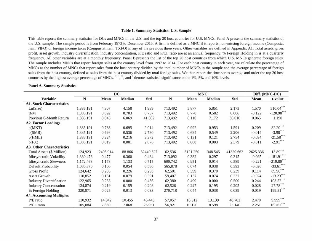
37

Table 1. Summary Statistics: U.S. Sample

This table reports the summary statistics for DCs and MNCs in the U.S. and the top 20 host countries for U.S. MNCs. Panel A presents the summary statistics of the U.S. sample. The sample period is from February 1973 to December 2015. A firm is defined as a MNC if it reports non-missing foreign income (Compustat item: PIFO) or foreign income taxes (Compustat item: TXFO) in any of the previous three years. Other variables are defined in Appendix A1. Total assets, gross profit, asset growth, industry diversification, industry concentration, P/E ratio and P/CF ratio are at an annual frequency. % Foreign Holding in is at a quarterly frequency. All other variables are at a monthly frequency. Panel B presents the list of the top 20 host countries from which U.S. MNCs generate foreign sales. The sample includes MNCs that report foreign sales at the country level from 1997 to 2014. For each host country in each year, we calculate the percentage of MNCs as the number of MNCs that report sales from the host country divided by the total number of MNCs in the sample and the average percentage of foreign sales from the host country, defined as sales from the host country divided by total foreign sales. We then report the time-series average and order the top 20 host countries by the highest average percentage of MNCs. ***, **, and * denote statistical significance at the 1%, 5% and 10% levels.

Panel A. Summary Statistics

DC MNC Diff. (MNC-DC) Variable N Mean Median Std N Mean Median Std Mean t-value

A1. Stock Characteristics Ln(Size) 1,385,191 4.307 4.158 1.989 713,492 5.877 5.851 2.173 1.570 510.04*** B/M 1,385,191 0.892 0.703 0.737 713,492 0.770 0.582 0.666 -0.122 -120.98*** Previous 6-Month Return 1,385,191 8.045 6.069 41.082 713,492 8.110 7.172 36.010 0.065 1.190

A2. Factor Loadings b(MKT) 1,385,191 0.783 0.695 2.014 713,492 0.992 0.953 1.591 0.209 82.20*** b(SMB) 1,385,191 0.698 0.536 2.730 713,492 0.684 0.549 2.206 -0.014 -3.98*** b(HML) 1,385,191 0.224 0.216 3.372 713,492 0.131 0.121 2.754 -0.094 -21.58*** b(FX) 1,385,191 0.019 0.001 2.876 713,492 0.008 0.003 2.379 -0.011 -2.91***

A3. Other Characteristics Total Assets ($ Million) 124,923 2495.914 88.866 32440.527 62,536 5121.250 348.545 41320.662 2625.336 13.89*** Idiosyncratic Volatility 1,380,476 0.477 0.360 0.434 713,092 0.382 0.297 0.315 -0.095 -181.91*** Idiosyncratic Skewness 1,172,463 1.173 1.133 0.715 600,742 0.951 0.914 0.589 -0.221 -219.80*** Default Probability 1,080,370 0.100 0.054 0.586 565,878 0.074 0.038 0.393 -0.026 -33.61*** Gross Profit 124,642 0.285 0.226 0.293 62,501 0.399 0.370 0.239 0.114 89.96*** Asset Growth 110,852 0.161 0.079 0.391 59,407 0.137 0.074 0.337 -0.024 -13.23*** Industry Diversification 122,965 0.255 0.000 0.436 62,380 0.499 0.000 0.500 0.244 103.52*** Industry Concentration 124,874 0.219 0.159 0.203 62,526 0.247 0.195 0.205 0.028 27.78*** % Foreign Holding 320,871 0.025 0.013 0.033 270,718 0.044 0.038 0.039 0.019 199.51***

A4. Accounting Multiples P/E ratio 110,932 14.042 10.455 46.443 57,057 16.512 13.139 48.702 2.470 9.999*** P/CF ratio 105,084 7.869 7.068 26.951 56,921 10.120 8.598 25.140 2.251 16.767***

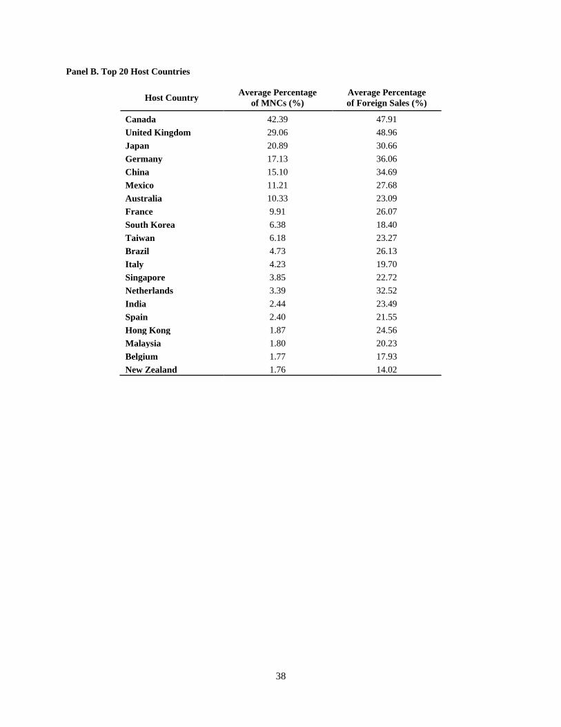
38

Panel B. Top 20 Host Countries

Host Country Average Percentage of MNCs (%)

Average Percentage of Foreign Sales (%)

Canada 42.39 47.91 United Kingdom 29.06 48.96 Japan 20.89 30.66 Germany 17.13 36.06 China 15.10 34.69 Mexico 11.21 27.68 Australia 10.33 23.09 France 9.91 26.07 South Korea 6.38 18.40 Taiwan 6.18 23.27 Brazil 4.73 26.13 Italy 4.23 19.70 Singapore 3.85 22.72 Netherlands 3.39 32.52 India 2.44 23.49 Spain 2.40 21.55 Hong Kong 1.87 24.56 Malaysia 1.80 20.23 Belgium 1.77 17.93 New Zealand 1.76 14.02

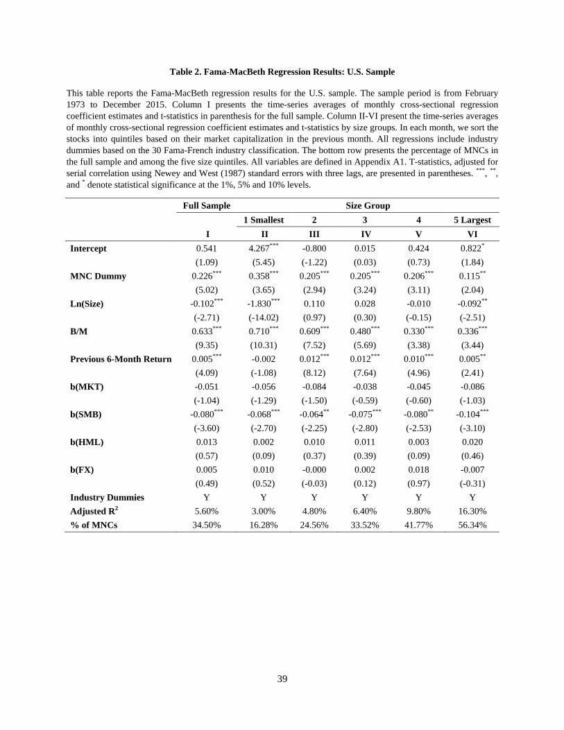
39

Table 2. Fama-MacBeth Regression Results: U.S. Sample

This table reports the Fama-MacBeth regression results for the U.S. sample. The sample period is from February 1973 to December 2015. Column I presents the time-series averages of monthly cross-sectional regression coefficient estimates and t-statistics in parenthesis for the full sample. Column II-VI present the time-series averages of monthly cross-sectional regression coefficient estimates and t-statistics by size groups. In each month, we sort the stocks into quintiles based on their market capitalization in the previous month. All regressions include industry dummies based on the 30 Fama-French industry classification. The bottom row presents the percentage of MNCs in the full sample and among the five size quintiles. All variables are defined in Appendix A1. T-statistics, adjusted for serial correlation using Newey and West (1987) standard errors with three lags, are presented in parentheses. ***, **, and * denote statistical significance at the 1%, 5% and 10% levels.

Full Sample Size Group

1 Smallest 2 3 4 5 Largest

I II III IV V VI Intercept 0.541 4.267*** -0.800 0.015 0.424 0.822*

(1.09) (5.45) (-1.22) (0.03) (0.73) (1.84) MNC Dummy 0.226*** 0.358*** 0.205*** 0.205*** 0.206*** 0.115**

(5.02) (3.65) (2.94) (3.24) (3.11) (2.04) Ln(Size) -0.102*** -1.830*** 0.110 0.028 -0.010 -0.092**

(-2.71) (-14.02) (0.97) (0.30) (-0.15) (-2.51) B/M 0.633*** 0.710*** 0.609*** 0.480*** 0.330*** 0.336***

(9.35) (10.31) (7.52) (5.69) (3.38) (3.44) Previous 6-Month Return 0.005*** -0.002 0.012*** 0.012*** 0.010*** 0.005**

(4.09) (-1.08) (8.12) (7.64) (4.96) (2.41) b(MKT) -0.051 -0.056 -0.084 -0.038 -0.045 -0.086

(-1.04) (-1.29) (-1.50) (-0.59) (-0.60) (-1.03) b(SMB) -0.080*** -0.068*** -0.064** -0.075*** -0.080** -0.104***

(-3.60) (-2.70) (-2.25) (-2.80) (-2.53) (-3.10) b(HML) 0.013 0.002 0.010 0.011 0.003 0.020

(0.57) (0.09) (0.37) (0.39) (0.09) (0.46) b(FX) 0.005 0.010 -0.000 0.002 0.018 -0.007

(0.49) (0.52) (-0.03) (0.12) (0.97) (-0.31) Industry Dummies Y Y Y Y Y Y Adjusted R2 5.60% 3.00% 4.80% 6.40% 9.80% 16.30% % of MNCs 34.50% 16.28% 24.56% 33.52% 41.77% 56.34%

40

Table 3. Alternative Explanations and Robustness: U.S. Sample

This table examines alternative explanations and robustness of MNC return premium for the U.S. sample. Panel A reports the Fama-MacBeth regression results with additional control variables, including idiosyncratic volatility, idiosyncratic skewness, default probability, gross profit, asset growth, industry diversification, industry concentration and % foreign holding. Panel B presents the coefficients and t-stats of the MNC dummy, the average number of firms, and the average percentage of MNCs for each 10-year subperiod, the financial crisis period between 2007Q3 and 2009Q1, the non-financial crisis period during 2004-2015 and (non) NBER recessions, based on Model I in Table 2. Panel C presents the performance of MNC and DC portfolios from time-series regressions for the full sample and by size group. In each month, we form portfolios based on the MNC status in the previous month and calculate the value-weighted excess returns, FF3 alpha, and FF4 alpha. FF3 alpha is the intercept from a regression of monthly excess return on Fama-French three factors. FF4 alpha is the intercept from a regression of monthly excess return on Fama-French three factors and momentum. All variables are defined in Appendix A1. T-statistics, adjusted for serial correlation using Newey and West (1987) standard errors with three lags, are presented in parentheses. ***, **, and * denote statistical significance at the 1%, 5% and 10% levels.

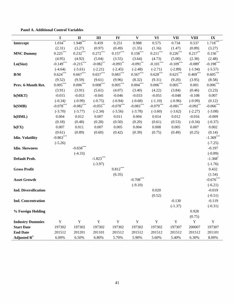
41

Panel A. Additional Control Variables

I II III IV V VI VII VIII IX Intercept 1.034** 1.948*** 0.459 0.251 0.988 0.575 0.734 0.537 1.718***

(2.31) (3.27) (0.97) (0.49) (1.35) (1.16) (1.47) (0.89) (3.27) MNC Dummy 0.225*** 0.232*** 0.272*** 0.157*** 0.158*** 0.211*** 0.226*** 0.217** 0.156**

(4.95) (4.92) (5.04) (3.55) (3.64) (4.73) (5.00) (2.38) (2.48) Ln(Size) -0.149*** -0.215*** -0.082** -0.093** -0.091** -0.101*** -0.109*** -0.089* -0.198***

(-4.64) (-5.61) (-2.21) (-2.45) (-2.48) (-2.71) (-2.89) (-1.94) (-5.57) B/M 0.624*** 0.667*** 0.657*** 0.683*** 0.567*** 0.628*** 0.625*** 0.469*** 0.605***

(9.52) (9.59) (9.61) (9.96) (8.32) (9.31) (9.20) (3.95) (8.58) Prev. 6-Month Ret. 0.005*** 0.006*** 0.008*** 0.005*** 0.004*** 0.006*** 0.005*** 0.001 0.006***

(3.91) (3.91) (5.61) (4.07) (3.40) (4.22) (3.84) (0.46) (3.23) b(MKT) -0.015 -0.053 -0.041 -0.046 -0.033 -0.055 -0.048 -0.108 0.007

(-0.34) (-0.99) (-0.75) (-0.94) (-0.68) (-1.10) (-0.96) (-0.99) (0.12) b(SMB) -0.078*** -0.082*** -0.055** -0.078*** -0.083*** -0.079*** -0.081*** -0.092** -0.066***

(-3.70) (-3.77) (-2.34) (-3.56) (-3.78) (-3.60) (-3.62) (-2.27) (-3.08) b(HML) 0.004 0.012 0.007 0.011 0.004 0.014 0.012 -0.016 -0.009

(0.18) (0.48) (0.28) (0.50) (0.20) (0.61) (0.53) (-0.34) (-0.37) b(FX) 0.007 0.011 0.007 0.005 0.004 0.008 0.005 0.007 0.002

(0.61) (0.89) (0.60) (0.42) (0.39) (0.75) (0.49) (0.25) (0.14) Idio. Volatility -0.863*** -1.369***

(-5.26) (-7.25) Idio. Skewness -0.658*** -0.197

(-4.33) (-0.89) Default Prob. -1.823*** -1.368*

(-3.97) (-1.76) Gross Profit 0.812*** 0.432

(6.35) (1.54) Asset Growth -0.708*** -0.676*** (-9.10) (-6.21) Ind. Diversification 0.020 -0.019

(0.52) (-0.51) Ind. Concentration -0.130 -0.119

(-1.37) (-0.31) % Foreign Holding 0.928 (0.75) Industry Dummies Y Y Y Y Y Y Y Y Y Start Date 197302 197302 197302 197302 197302 197302 197307 200007 197307 End Date 201512 201201 201101 201512 201512 201512 201512 201512 201101 Adjusted R2 6.00% 6.50% 6.80% 5.70% 5.90% 5.60% 5.40% 6.30% 8.00%

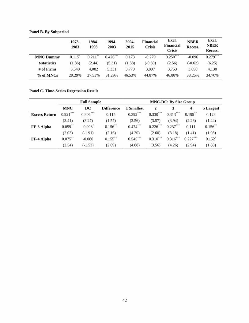
42

Panel B. By Subperiod

1973-1983

1984-1993

1994-2003

2004-2015

Financial Crisis

Excl. Financial

Crisis

NBER Recess.

Excl. NBER Recess.

MNC Dummy 0.115* 0.211** 0.426*** 0.173 -0.279 0.250*** -0.096 0.279*** t-statistics (1.86) (2.44) (5.31) (1.58) (-0.60) (2.56) (-0.62) (6.25) # of Firms 3,349 4,082 5,331 3,779 3,897 3,753 3,690 4,138

% of MNCs 29.29% 27.53% 31.29% 46.53% 44.87% 46.88% 33.25% 34.70%

Panel C. Time-Series Regression Result

Full Sample MNC-DC: By Size Group

MNC DC Difference 1 Smallest 2 3 4 5 Largest Excess Return 0.921*** 0.806*** 0.115 0.392*** 0.330*** 0.313*** 0.199** 0.128

(3.41) (3.27) (1.57) (3.56) (3.57) (3.94) (2.26) (1.44) FF-3 Alpha 0.059** -0.098* 0.156** 0.474*** 0.226*** 0.237*** 0.111 0.156**

(2.03) (-1.91) (2.16) (4.30) (2.60) (3.18) (1.41) (1.98) FF-4 Alpha 0.075** -0.080 0.155** 0.545*** 0.310*** 0.316*** 0.227*** 0.152* (2.54) (-1.53) (2.09) (4.88) (3.56) (4.26) (2.94) (1.88)

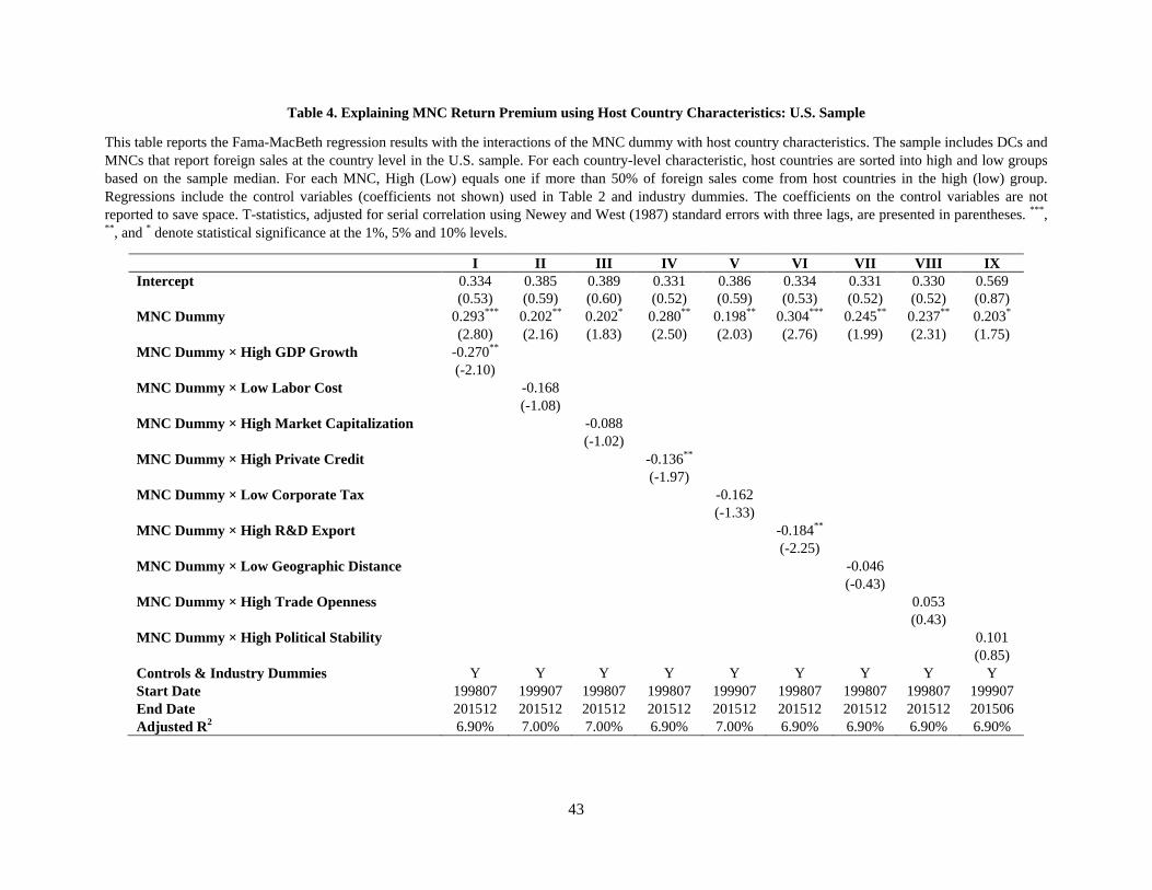
43

Table 4. Explaining MNC Return Premium using Host Country Characteristics: U.S. Sample

This table reports the Fama-MacBeth regression results with the interactions of the MNC dummy with host country characteristics. The sample includes DCs and MNCs that report foreign sales at the country level in the U.S. sample. For each country-level characteristic, host countries are sorted into high and low groups based on the sample median. For each MNC, High (Low) equals one if more than 50% of foreign sales come from host countries in the high (low) group. Regressions include the control variables (coefficients not shown) used in Table 2 and industry dummies. The coefficients on the control variables are not reported to save space. T-statistics, adjusted for serial correlation using Newey and West (1987) standard errors with three lags, are presented in parentheses. ***, **, and * denote statistical significance at the 1%, 5% and 10% levels.

I II III IV V VI VII VIII IX Intercept 0.334 0.385 0.389 0.331 0.386 0.334 0.331 0.330 0.569

(0.53) (0.59) (0.60) (0.52) (0.59) (0.53) (0.52) (0.52) (0.87) MNC Dummy 0.293*** 0.202** 0.202* 0.280** 0.198** 0.304*** 0.245** 0.237** 0.203*

(2.80) (2.16) (1.83) (2.50) (2.03) (2.76) (1.99) (2.31) (1.75) MNC Dummy × High GDP Growth -0.270**

(-2.10)

MNC Dummy × Low Labor Cost -0.168

(-1.08) MNC Dummy × High Market Capitalization -0.088

(-1.02) MNC Dummy × High Private Credit -0.136**

(-1.97) MNC Dummy × Low Corporate Tax -0.162

(-1.33) MNC Dummy × High R&D Export -0.184**

(-2.25) MNC Dummy × Low Geographic Distance -0.046

(-0.43) MNC Dummy × High Trade Openness 0.053

(0.43) MNC Dummy × High Political Stability 0.101 (0.85) Controls & Industry Dummies Y Y Y Y Y Y Y Y Y Start Date 199807 199907 199807 199807 199907 199807 199807 199807 199907 End Date 201512 201512 201512 201512 201512 201512 201512 201512 201506 Adjusted R2 6.90% 7.00% 7.00% 6.90% 7.00% 6.90% 6.90% 6.90% 6.90%

44

Table 5. Summary Statistics: Global Sample

This table reports the summary statistics of the global sample. Panel A presents the number of MNCs and DCs, the percentage of MNCs, the percentage of globally accessible firms, and the average of market capitalization by country. The global sample includes firms from 23 developed markets as defined by MSCI. The sample period is from January 1990 to December 2015. A firm is defined as a MNC if it reports non-missing foreign income (Worldscope item: WC08741) in any of the previous three years. For each country in each year, we obtain the number of MNCs and DCs, the percentage of MNCs in terms of numbers, the percentage of globally accessible firms, and the average market capitalization of MNCs and DCs (in $ millions), and the percentage of MNCs in terms of market capitalization. We then report the time-series average over the sample period for each country. Panel B presents the summary statistics for the global sample. All variables are defined in the Appendix A1. Gross profit, asset growth, and globally accessible are reported at an annual frequency. All other variables are at a monthly frequency. ***, **, and * denote statistical significance at the 1%, 5% and 10% levels. Panel C presents the list of top 20 host countries from which MNCs in the global sample generate foreign sales. The sample includes MNCs that report foreign sales at the country level from 2000 to 2015. For each host country in each year, we calculate the percentage of MNCs that have positive foreign sales from each host country and the percentage of foreign sales from the host country. We then report the time-series averages and host countries are sorted in the descending order of the percentage of MNCs with foreign sales. Panel A. The percentage of MNCs

Number of Firms Market Capitalization (in $Millions)

Country MNC DC % of MNCs

% of Globally Accessible MNC DC % of MNCs

Australia 183.81 651.81 29.32 47.84 1391.21 539.53 72.21 Austria 23.07 58.86 28.34 65.90 2194.56 987.17 69.67 Belgium 18.42 87.00 17.48 100.00 8005.08 1570.41 82.73 Canada 151.04 933.42 22.28 69.31 3006.26 578.42 74.48 Denmark 16.75 133.42 11.16 26.99 1693.98 1185.77 57.87 Finland 17.64 102.09 14.79 54.93 1073.84 1639.35 36.78 France 76.27 497.50 12.53 97.17 6282.04 1762.26 75.48 Germany 68.75 592.60 9.89 86.68 9660.38 1330.38 84.72 Hong Kong 218.23 462.62 36.78 99.81 1636.77 1122.79 54.77 Ireland 18.24 33.24 35.02 88.50 1689.91 734.19 73.88 Israel 14.47 209.42 8.82 44.07 1366.76 476.94 69.13 Italy 28.20 208.20 11.99 49.96 4842.97 2229.80 66.48 Japan 540.60 2696.95 16.67 25.96 3165.18 678.77 81.99 Netherlands 21.45 103.05 18.62 99.35 10235.25 3472.28 74.98 New Zealand 19.83 57.33 26.74 36.78 615.41 367.08 61.02 Norway 17.00 153.79 9.53 49.77 1861.36 1019.62 63.87 Portugal 10.55 34.91 23.45 100.00 3211.96 1417.23 65.42 Singapore 95.00 295.46 33.92 100.00 1339.48 588.57 62.80 Spain 22.60 101.60 18.17 61.66 11373.91 3901.28 73.84 Sweden 30.50 284.56 8.87 38.67 2661.53 1107.62 70.28 Switzerland 28.64 174.59 13.44 61.79 10411.99 3046.77 77.65 United Kingdom 423.31 868.12 32.59 98.90 3387.89 686.58 83.28 United States 1739.46 3105.77 37.77 100.00 4810.53 1289.91 79.39

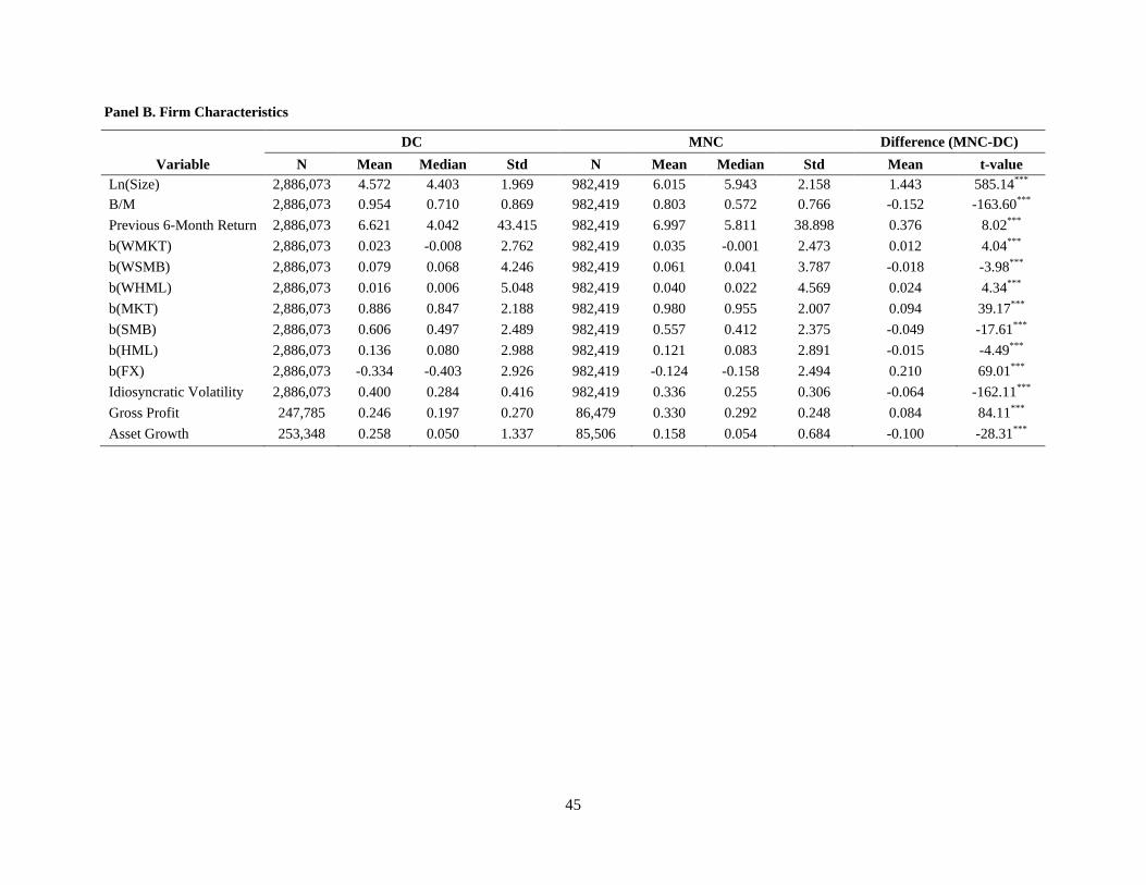
45

Panel B. Firm Characteristics

DC MNC Difference (MNC-DC) Variable N Mean Median Std N Mean Median Std Mean t-value

Ln(Size) 2,886,073 4.572 4.403 1.969 982,419 6.015 5.943 2.158 1.443 585.14*** B/M 2,886,073 0.954 0.710 0.869 982,419 0.803 0.572 0.766 -0.152 -163.60*** Previous 6-Month Return 2,886,073 6.621 4.042 43.415 982,419 6.997 5.811 38.898 0.376 8.02*** b(WMKT) 2,886,073 0.023 -0.008 2.762 982,419 0.035 -0.001 2.473 0.012 4.04*** b(WSMB) 2,886,073 0.079 0.068 4.246 982,419 0.061 0.041 3.787 -0.018 -3.98*** b(WHML) 2,886,073 0.016 0.006 5.048 982,419 0.040 0.022 4.569 0.024 4.34*** b(MKT) 2,886,073 0.886 0.847 2.188 982,419 0.980 0.955 2.007 0.094 39.17*** b(SMB) 2,886,073 0.606 0.497 2.489 982,419 0.557 0.412 2.375 -0.049 -17.61*** b(HML) 2,886,073 0.136 0.080 2.988 982,419 0.121 0.083 2.891 -0.015 -4.49*** b(FX) 2,886,073 -0.334 -0.403 2.926 982,419 -0.124 -0.158 2.494 0.210 69.01*** Idiosyncratic Volatility 2,886,073 0.400 0.284 0.416 982,419 0.336 0.255 0.306 -0.064 -162.11*** Gross Profit 247,785 0.246 0.197 0.270 86,479 0.330 0.292 0.248 0.084 84.11*** Asset Growth 253,348 0.258 0.050 1.337 85,506 0.158 0.054 0.684 -0.100 -28.31***

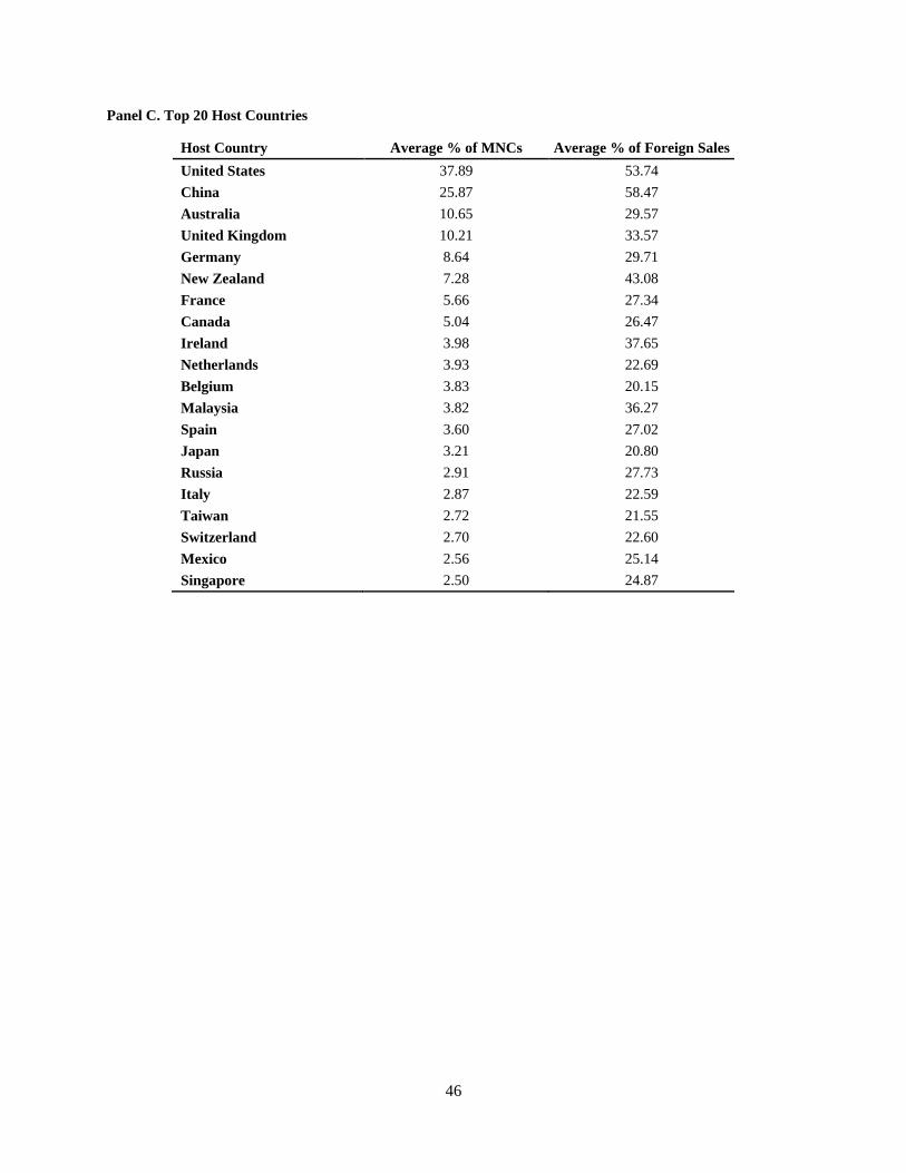
46

Panel C. Top 20 Host Countries

Host Country Average % of MNCs Average % of Foreign Sales United States 37.89 53.74 China 25.87 58.47 Australia 10.65 29.57 United Kingdom 10.21 33.57 Germany 8.64 29.71 New Zealand 7.28 43.08 France 5.66 27.34 Canada 5.04 26.47 Ireland 3.98 37.65 Netherlands 3.93 22.69 Belgium 3.83 20.15 Malaysia 3.82 36.27 Spain 3.60 27.02 Japan 3.21 20.80 Russia 2.91 27.73 Italy 2.87 22.59 Taiwan 2.72 21.55 Switzerland 2.70 22.60 Mexico 2.56 25.14 Singapore 2.50 24.87

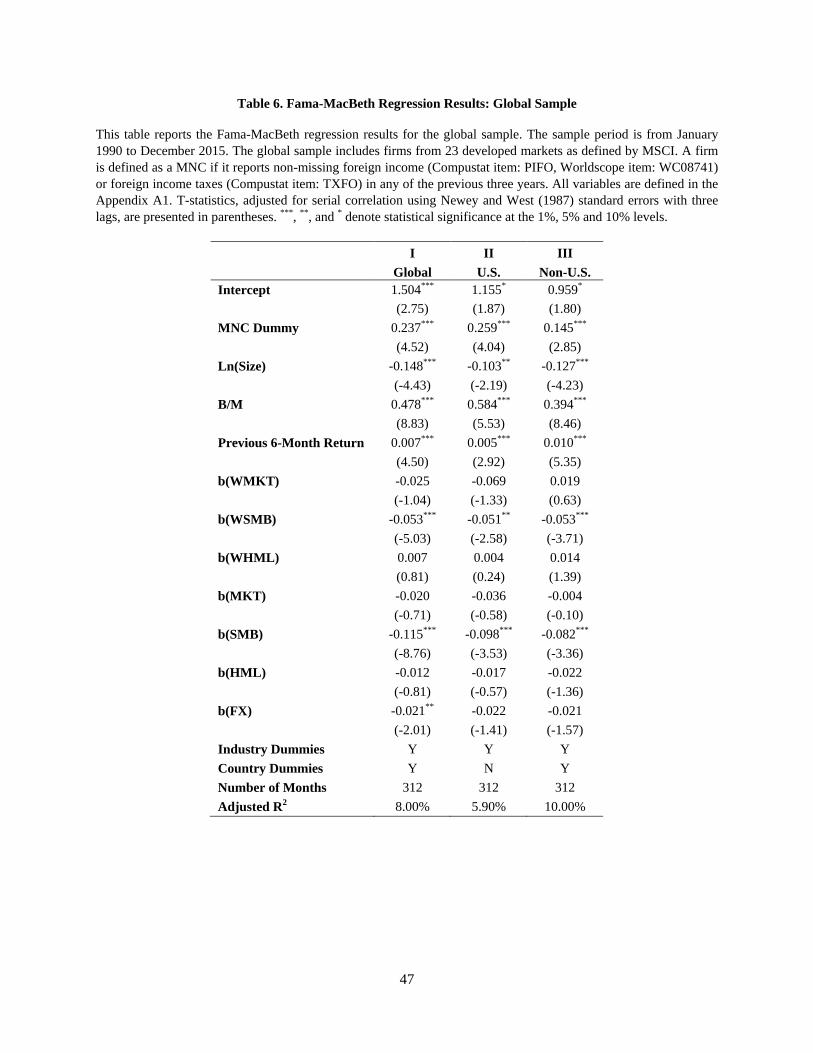
47

Table 6. Fama-MacBeth Regression Results: Global Sample

This table reports the Fama-MacBeth regression results for the global sample. The sample period is from January 1990 to December 2015. The global sample includes firms from 23 developed markets as defined by MSCI. A firm is defined as a MNC if it reports non-missing foreign income (Compustat item: PIFO, Worldscope item: WC08741) or foreign income taxes (Compustat item: TXFO) in any of the previous three years. All variables are defined in the Appendix A1. T-statistics, adjusted for serial correlation using Newey and West (1987) standard errors with three lags, are presented in parentheses. ***, **, and * denote statistical significance at the 1%, 5% and 10% levels.

I II III

Global U.S. Non-U.S.

Intercept 1.504*** 1.155* 0.959*

(2.75) (1.87) (1.80) MNC Dummy 0.237*** 0.259*** 0.145*** (4.52) (4.04) (2.85) Ln(Size) -0.148*** -0.103** -0.127***

(-4.43) (-2.19) (-4.23) B/M 0.478*** 0.584*** 0.394***

(8.83) (5.53) (8.46) Previous 6-Month Return 0.007*** 0.005*** 0.010***

(4.50) (2.92) (5.35) b(WMKT) -0.025 -0.069 0.019

(-1.04) (-1.33) (0.63) b(WSMB) -0.053*** -0.051** -0.053***

(-5.03) (-2.58) (-3.71) b(WHML) 0.007 0.004 0.014

(0.81) (0.24) (1.39) b(MKT) -0.020 -0.036 -0.004

(-0.71) (-0.58) (-0.10) b(SMB) -0.115*** -0.098*** -0.082***

(-8.76) (-3.53) (-3.36) b(HML) -0.012 -0.017 -0.022

(-0.81) (-0.57) (-1.36) b(FX) -0.021** -0.022 -0.021

(-2.01) (-1.41) (-1.57) Industry Dummies Y Y Y Country Dummies Y N Y Number of Months 312 312 312 Adjusted R2 8.00% 5.90% 10.00%

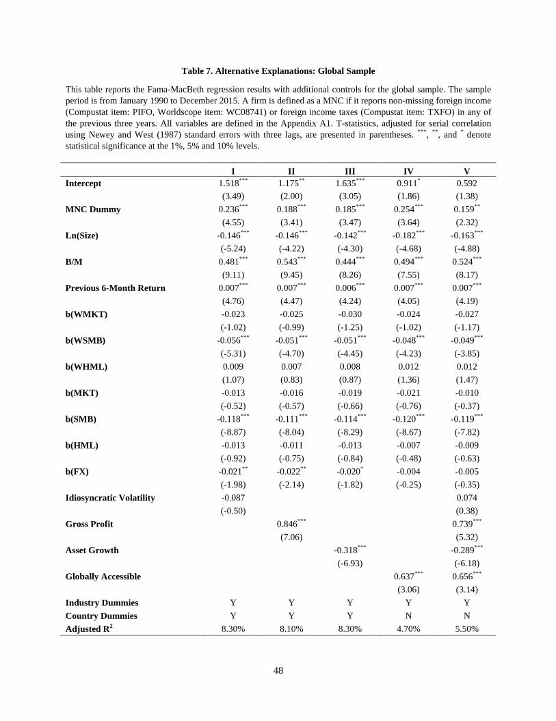
48

Table 7. Alternative Explanations: Global Sample

This table reports the Fama-MacBeth regression results with additional controls for the global sample. The sample period is from January 1990 to December 2015. A firm is defined as a MNC if it reports non-missing foreign income (Compustat item: PIFO, Worldscope item: WC08741) or foreign income taxes (Compustat item: TXFO) in any of the previous three years. All variables are defined in the Appendix A1. T-statistics, adjusted for serial correlation using Newey and West (1987) standard errors with three lags, are presented in parentheses. ***, **, and * denote statistical significance at the 1%, 5% and 10% levels.

I II III IV V Intercept 1.518*** 1.175** 1.635*** 0.911* 0.592

(3.49) (2.00) (3.05) (1.86) (1.38) MNC Dummy 0.236*** 0.188*** 0.185*** 0.254*** 0.159**

(4.55) (3.41) (3.47) (3.64) (2.32) Ln(Size) -0.146*** -0.146*** -0.142*** -0.182*** -0.163***

(-5.24) (-4.22) (-4.30) (-4.68) (-4.88) B/M 0.481*** 0.543*** 0.444*** 0.494*** 0.524***

(9.11) (9.45) (8.26) (7.55) (8.17) Previous 6-Month Return 0.007*** 0.007*** 0.006*** 0.007*** 0.007***

(4.76) (4.47) (4.24) (4.05) (4.19) b(WMKT) -0.023 -0.025 -0.030 -0.024 -0.027

(-1.02) (-0.99) (-1.25) (-1.02) (-1.17) b(WSMB) -0.056*** -0.051*** -0.051*** -0.048*** -0.049***

(-5.31) (-4.70) (-4.45) (-4.23) (-3.85) b(WHML) 0.009 0.007 0.008 0.012 0.012

(1.07) (0.83) (0.87) (1.36) (1.47) b(MKT) -0.013 -0.016 -0.019 -0.021 -0.010

(-0.52) (-0.57) (-0.66) (-0.76) (-0.37) b(SMB) -0.118*** -0.111*** -0.114*** -0.120*** -0.119***

(-8.87) (-8.04) (-8.29) (-8.67) (-7.82) b(HML) -0.013 -0.011 -0.013 -0.007 -0.009

(-0.92) (-0.75) (-0.84) (-0.48) (-0.63) b(FX) -0.021** -0.022** -0.020* -0.004 -0.005

(-1.98) (-2.14) (-1.82) (-0.25) (-0.35) Idiosyncratic Volatility -0.087 0.074

(-0.50) (0.38) Gross Profit 0.846*** 0.739***

(7.06) (5.32) Asset Growth -0.318*** -0.289*** (-6.93) (-6.18) Globally Accessible 0.637*** 0.656***

(3.06) (3.14) Industry Dummies Y Y Y Y Y Country Dummies Y Y Y N N Adjusted R2 8.30% 8.10% 8.30% 4.70% 5.50%

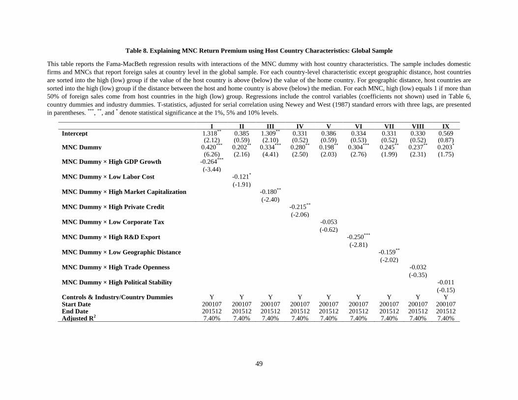
49

Table 8. Explaining MNC Return Premium using Host Country Characteristics: Global Sample

This table reports the Fama-MacBeth regression results with interactions of the MNC dummy with host country characteristics. The sample includes domestic firms and MNCs that report foreign sales at country level in the global sample. For each country-level characteristic except geographic distance, host countries are sorted into the high (low) group if the value of the host country is above (below) the value of the home country. For geographic distance, host countries are sorted into the high (low) group if the distance between the host and home country is above (below) the median. For each MNC, high (low) equals 1 if more than 50% of foreign sales come from host countries in the high (low) group. Regressions include the control variables (coefficients not shown) used in Table 6, country dummies and industry dummies. T-statistics, adjusted for serial correlation using Newey and West (1987) standard errors with three lags, are presented in parentheses. ***, **, and * denote statistical significance at the 1%, 5% and 10% levels.

I II III IV V VI VII VIII IX Intercept 1.318** 0.385 1.309** 0.331 0.386 0.334 0.331 0.330 0.569 (2.12) (0.59) (2.10) (0.52) (0.59) (0.53) (0.52) (0.52) (0.87) MNC Dummy 0.420*** 0.202** 0.334*** 0.280** 0.198** 0.304*** 0.245** 0.237** 0.203* (6.26) (2.16) (4.41) (2.50) (2.03) (2.76) (1.99) (2.31) (1.75) MNC Dummy × High GDP Growth -0.264***

(-3.44)

MNC Dummy × Low Labor Cost -0.121*

(-1.91) MNC Dummy × High Market Capitalization -0.180**

(-2.40) MNC Dummy × High Private Credit -0.215**

(-2.06) MNC Dummy × Low Corporate Tax -0.053

(-0.62) MNC Dummy × High R&D Export -0.250***

(-2.81) MNC Dummy × Low Geographic Distance -0.159**

(-2.02) MNC Dummy × High Trade Openness -0.032

(-0.35) MNC Dummy × High Political Stability -0.011 (-0.15) Controls & Industry/Country Dummies Y Y Y Y Y Y Y Y Y Start Date 200107 200107 200107 200107 200107 200107 200107 200107 200107 End Date 201512 201512 201512 201512 201512 201512 201512 201512 201512 Adjusted R2 7.40% 7.40% 7.40% 7.40% 7.40% 7.40% 7.40% 7.40% 7.40%

50

Appendix

A1. Variable Description

Variable Description

MNC Dummy For U.S. firms, this variable equals 1 if the firm reports non-missing foreign income (Compustat item: PIFO) or foreign income taxes (Compustat item: TXFO) in any of the previous three years and 0 otherwise. For non-U.S. firms, this variable equals 1 if the firm reports non-missing foreign income (Worldscope item: WC08741) in any of the previous three years, and 0 otherwise.

Excess Return U.S. dollar-denominated stock return (from Datastream) minus U.S. T-bill rate (from Kenneth R. French Data Library), multiplied by 100.

Ln (Size) The natural logarithm of market value, in US$ millions. B/M Book equity divided by market value of equity. The market value of equity from July of

year t to June of year t + 1 is matched to the book equity at the end of year t − 1.

Previous 6-Month Return The sum of monthly returns in the previous 6 months. Idiosyncratic Volatility For the U.S. sample, idiosyncratic volatility is the annualized volatility of the residuals

from the regressions using the Fama-French three factor model (Ang et al. (2009)).

For the global sample, idiosyncratic volatility is estimated from the regressions using the global-local Fama-French three factor model as in Bekaert, Hodrick and Zhang (2009).

Idiosyncratic Skewness Expected idiosyncratic skewness, from Brian Boyer’s website

http://marriottschool.net/emp/boyer/Research/skewdata.html

Default Probability Measure of default risk from Vassalou and Xing (2004). b(MKT), b(SMB), b(HML), b(WMKT), b(WSMB), b(WHML)

For the U.S. sample, b(MKT), b(SMB), and b(HML), are the loadings on MKT, SMB, and HML factors, respectively, from the monthly regression of daily excess return on the Fama-French three factors (from the Kenneth R. French Data Library).

For the global sample, b(MKT) , b(SMB), b(HML), b(WMKT) , b(WSMB), and b(WHML) are the loadings on the local and global factors, respectively, from the monthly regression of daily excess return on global and local MKT factors or from the monthly regression of daily excess return on the global and local Fama-French three factors.

Local MKT factor is the value-weighted return of all firms in the country, where the weight equals the lagged market value of each stock in that country. The global MKT factor, WMKT, is the value weighted sum of local MKT factors for all countries, where the weight equals the lagged market value of all stocks in each country.

To obtain the local SMB factors at country level, we sort all firms in that country into three size groups in each month based on the 6-month lagged market value and calculate SMB as the value-weighted return difference between firms in size group 1 (smallest) and size group 3 (largest). The global SMB factor, WSMB, is the value weighted sum of local SMB factors for all countries, where the weight equals the lagged market value of all stocks in each country.

Similarly, the local HML factor is the value-weighted return difference between firms in B/M group 3 (highest) and B/M group 1 (lowest). The global HML factor, WHML, is the value weighted sum of local HML factors for all countries, where the weight equals the lagged market value of all stocks in each country.

51

b(FX) For the U.S. sample, b(FX) is the loading on the foreign exchange factor, FX, from the monthly regression of daily excess return on the MKT factor and FX factor.

For the global sample, b(FX) is the loading on the FX factor from the monthly regression of daily excess return on the local MKT factor, global MKT factor (WMKT) and FX factor.

The FX factor is the return of the trade weighted U.S. dollar index (major currencies) from the Federal Reserve Bank of St. Louis.

Gross Profit For the U.S. sample, this variable is defined as revenues minus cost of goods sold (REVT − COGS) scaled by total assets (AT) (Source: Compustat). For the global sample, it is defined as (WC01001 – WC01051)/WC02999 (Source: Worldscope).

Industry Diversification An indicator variable equal to one if the firm has more than one industry segment. (Source: Compustat Segment)

Industry Concentration A sales-based Herfindahl index (Hou and Robinson (2006)). Industry Concentration = ∑ 𝑐𝑐𝑖𝑖𝑖𝑖2𝑁𝑁𝑖𝑖=1 , where sij is the market share (in terms of sales) of firm i in industry j. Industries

are classified based on three-digit SIC codes. A larger value implies a higher industry concentration. (Source: Compustat)

Asset Growth The change in total assets (AT) scaled by lagged total assets. % Foreign Holding The percentage of foreign institutional holdings out of the total shares outstanding.

(Source: Thomson Reuter’s quarterly 13-F filings).

P/E Ratio Price to earnings ratio, calculated as market value at the end of June of t divided by income before extraordinary items during the last fiscal year ended in t-1.

P/CF Ratio Price to cash flow ratio, calculated as market value at the end of June of t divided by income before extraordinary items and depreciation during the last fiscal year ended in t-1.

GDP Growth The annual real growth rate of GDP. (Source: World Bank) GDP per capita The annual GDP (in U.S. dollars) divided by population. (Source: World Bank) Labor Cost Mean monthly labor costs per employee by country adjusted for PPI in USD. (Source:

OECD, International Labor Organization, web search)

Market Capitalization Market capitalization of listed domestic companies (% of GDP). (Source: World Bank) Private Credit Domestic credit to private sector (% of GDP). (Source: World Bank) Corporate Tax Highest corporate marginal income tax rate. (Source: OECD, World Bank, Worldwide Tax

Summaries from PwC)

R&D Export High-technology exports (% of manufactured exports). (Source: World Bank) Trade Openness The maximum of exports and imports of goods and services (% of GDP). (Source: World

Bank)

Geographic Distance The negative of the great circle distance between the capitals of home(i) and host(j) countries. We obtain latitude and longitude of capital cities of each country. 3963 * arccos [sin(lati) * sin(latj) + cos(lati) * cos(latj) * cos (lonj – loni)], where lon and lat are the longitudes and latitudes of the capitals of country i and j.

Political Stability The score on the political stability and absence of violence, scaled from zero (unstable) to one (stable). (Source: Political Risk Services International Country Risk Guide (PRS))

52

Globally Accessible A firm is globally accessible if it has stocks listed in any of the following markets: (i) the U.S., which includes NYSE/AMEX, NASDAQ, and the Non-NASDAQ OTC markets; (ii) the U.K., which includes the London Stock Exchange, London OTC Exchange, London Plus Market, and SEAQ International; (iii) Europe, which includes Euronext at Amsterdam, Brussels, Lisbon, Paris, and EASDAQ; (iv) Germany in which the Frankfurt Stock Exchange is located; (v) Luxembourg in which the Luxembourg Stock Exchange is located; (vi) Singapore, which includes the Singapore Stock Exchange, Singapore OTC Capital, and Singapore Catalist; and (vii) Hong Kong in which the Hong Kong Stock Exchange is located (Karoyli and Wu, 2012).

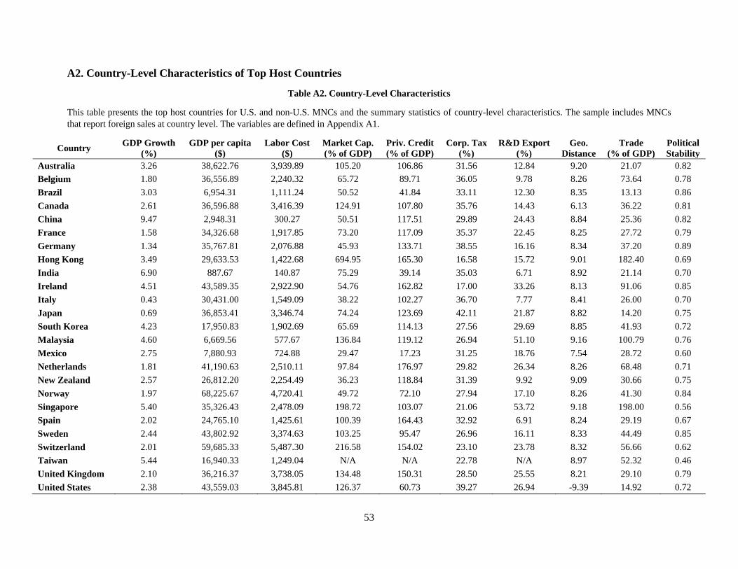
53

A2. Country-Level Characteristics of Top Host Countries

Table A2. Country-Level Characteristics

This table presents the top host countries for U.S. and non-U.S. MNCs and the summary statistics of country-level characteristics. The sample includes MNCs that report foreign sales at country level. The variables are defined in Appendix A1.

Country GDP Growth (%)

GDP per capita ($)

Labor Cost ($)

Market Cap. (% of GDP)

Priv. Credit (% of GDP)

Corp. Tax (%)

R&D Export (%)

Geo. Distance

Trade (% of GDP)

Political Stability

Australia 3.26 38,622.76 3,939.89 105.20 106.86 31.56 12.84 9.20 21.07 0.82 Belgium 1.80 36,556.89 2,240.32 65.72 89.71 36.05 9.78 8.26 73.64 0.78 Brazil 3.03 6,954.31 1,111.24 50.52 41.84 33.11 12.30 8.35 13.13 0.86 Canada 2.61 36,596.88 3,416.39 124.91 107.80 35.76 14.43 6.13 36.22 0.81 China 9.47 2,948.31 300.27 50.51 117.51 29.89 24.43 8.84 25.36 0.82 France 1.58 34,326.68 1,917.85 73.20 117.09 35.37 22.45 8.25 27.72 0.79 Germany 1.34 35,767.81 2,076.88 45.93 133.71 38.55 16.16 8.34 37.20 0.89 Hong Kong 3.49 29,633.53 1,422.68 694.95 165.30 16.58 15.72 9.01 182.40 0.69 India 6.90 887.67 140.87 75.29 39.14 35.03 6.71 8.92 21.14 0.70 Ireland 4.51 43,589.35 2,922.90 54.76 162.82 17.00 33.26 8.13 91.06 0.85 Italy 0.43 30,431.00 1,549.09 38.22 102.27 36.70 7.77 8.41 26.00 0.70 Japan 0.69 36,853.41 3,346.74 74.24 123.69 42.11 21.87 8.82 14.20 0.75 South Korea 4.23 17,950.83 1,902.69 65.69 114.13 27.56 29.69 8.85 41.93 0.72 Malaysia 4.60 6,669.56 577.67 136.84 119.12 26.94 51.10 9.16 100.79 0.76 Mexico 2.75 7,880.93 724.88 29.47 17.23 31.25 18.76 7.54 28.72 0.60 Netherlands 1.81 41,190.63 2,510.11 97.84 176.97 29.82 26.34 8.26 68.48 0.71 New Zealand 2.57 26,812.20 2,254.49 36.23 118.84 31.39 9.92 9.09 30.66 0.75 Norway 1.97 68,225.67 4,720.41 49.72 72.10 27.94 17.10 8.26 41.30 0.84 Singapore 5.40 35,326.43 2,478.09 198.72 103.07 21.06 53.72 9.18 198.00 0.56 Spain 2.02 24,765.10 1,425.61 100.39 164.43 32.92 6.91 8.24 29.19 0.67 Sweden 2.44 43,802.92 3,374.63 103.25 95.47 26.96 16.11 8.33 44.49 0.85 Switzerland 2.01 59,685.33 5,487.30 216.58 154.02 23.10 23.78 8.32 56.66 0.62 Taiwan 5.44 16,940.33 1,249.04 N/A N/A 22.78 N/A 8.97 52.32 0.46 United Kingdom 2.10 36,216.37 3,738.05 134.48 150.31 28.50 25.55 8.21 29.10 0.79 United States 2.38 43,559.03 3,845.81 126.37 60.73 39.27 26.94 -9.39 14.92 0.72

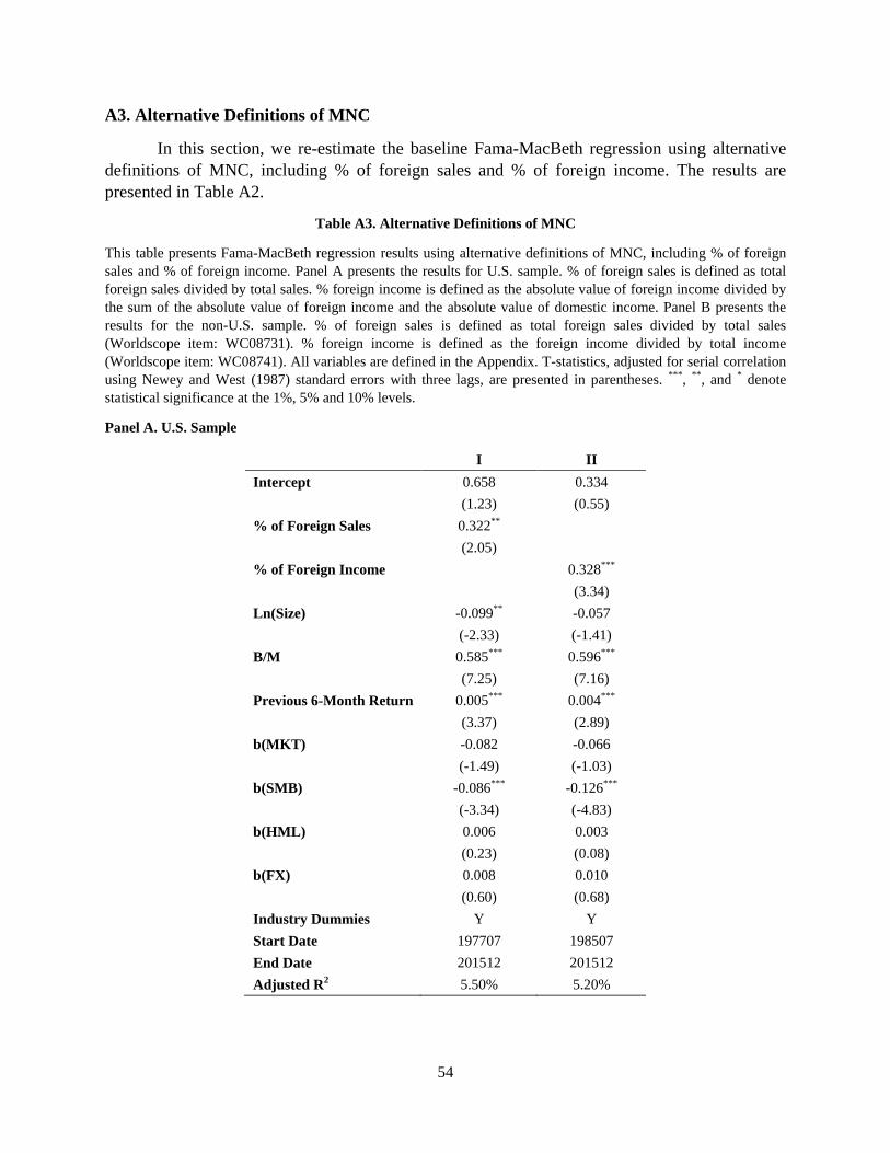
54

A3. Alternative Definitions of MNC

In this section, we re-estimate the baseline Fama-MacBeth regression using alternative definitions of MNC, including % of foreign sales and % of foreign income. The results are presented in Table A2.

Table A3. Alternative Definitions of MNC

This table presents Fama-MacBeth regression results using alternative definitions of MNC, including % of foreign sales and % of foreign income. Panel A presents the results for U.S. sample. % of foreign sales is defined as total foreign sales divided by total sales. % foreign income is defined as the absolute value of foreign income divided by the sum of the absolute value of foreign income and the absolute value of domestic income. Panel B presents the results for the non-U.S. sample. % of foreign sales is defined as total foreign sales divided by total sales (Worldscope item: WC08731). % foreign income is defined as the foreign income divided by total income (Worldscope item: WC08741). All variables are defined in the Appendix. T-statistics, adjusted for serial correlation using Newey and West (1987) standard errors with three lags, are presented in parentheses. ***, **, and * denote statistical significance at the 1%, 5% and 10% levels.

Panel A. U.S. Sample

I II Intercept 0.658 0.334

(1.23) (0.55) % of Foreign Sales 0.322** (2.05) % of Foreign Income 0.328*** (3.34) Ln(Size) -0.099** -0.057

(-2.33) (-1.41) B/M 0.585*** 0.596***

(7.25) (7.16) Previous 6-Month Return 0.005*** 0.004***

(3.37) (2.89) b(MKT) -0.082 -0.066

(-1.49) (-1.03) b(SMB) -0.086*** -0.126***

(-3.34) (-4.83) b(HML) 0.006 0.003

(0.23) (0.08) b(FX) 0.008 0.010

(0.60) (0.68) Industry Dummies Y Y Start Date 197707 198507 End Date 201512 201512 Adjusted R2 5.50% 5.20%

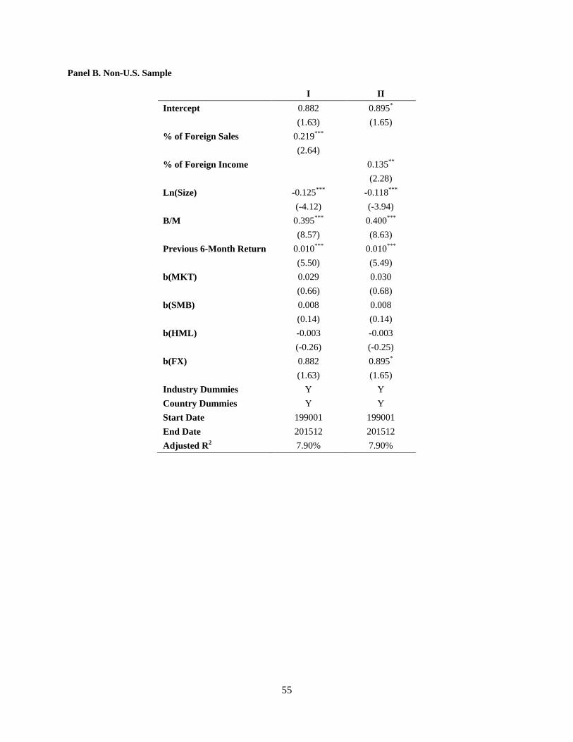
55

Panel B. Non-U.S. Sample

I II Intercept 0.882 0.895*

(1.63) (1.65) % of Foreign Sales 0.219***

(2.64) % of Foreign Income 0.135** (2.28) Ln(Size) -0.125*** -0.118***

(-4.12) (-3.94) B/M 0.395*** 0.400***

(8.57) (8.63) Previous 6-Month Return 0.010*** 0.010***

(5.50) (5.49) b(MKT) 0.029 0.030

(0.66) (0.68) b(SMB) 0.008 0.008

(0.14) (0.14) b(HML) -0.003 -0.003

(-0.26) (-0.25) b(FX) 0.882 0.895*

(1.63) (1.65) Industry Dummies Y Y Country Dummies Y Y Start Date 199001 199001 End Date 201512 201512 Adjusted R2 7.90% 7.90%

56

A4. Possible Channels of MNC Return Premium: Two-Stage Approach

When we include the MNC dummy and the other control variables in the same regression, it only

proves robustness rather than causality. To understand channels through which MNCs earn

higher returns than DCs, we further examine the possible driving forces for the higher returns

associated with MNCs in more depth by using a two-stage approach.

In the first stage, we project the MNC indicator variable on a possible channel as below:

𝑀𝑀𝑀𝑀𝑀𝑀𝑖𝑖,𝑡𝑡 = 𝑎𝑎𝑡𝑡 + 𝑏𝑏𝑡𝑡𝑝𝑝𝑟𝑟𝑐𝑐𝑝𝑝𝐶𝐶𝑖𝑖,𝑡𝑡 + 𝜀𝜀𝑖𝑖,𝑡𝑡 , (1)

where the proxy can be a variety of possible channels, such as idiosyncratic volatility or

profitability, that might be related or affect a firm’s multinational status. After we estimate the

specification above, we can decompose the MNC indicator into two parts:

𝑀𝑀𝑀𝑀𝑀𝑀𝑖𝑖,𝑡𝑡+1 = �𝑎𝑎�𝑡𝑡 + 𝑏𝑏�𝑡𝑡𝑝𝑝𝑟𝑟𝑐𝑐𝑝𝑝𝐶𝐶𝑖𝑖,𝑡𝑡+1� + 𝜀𝜀�̂�𝑖,𝑡𝑡+1 = 𝑋𝑋𝑀𝑀𝑀𝑀𝑀𝑀𝑖𝑖,𝑡𝑡+1 + 𝐸𝐸𝑀𝑀𝑀𝑀𝑀𝑀𝑖𝑖,𝑡𝑡+1. (2)

That is, XMNC represents the part of the MNC dummy predicted by (or associated with) a

potential channel, and EMNC is the part of the MNC dummy orthogonal to the potential channel.

At the second stage, we re-estimate the following predictive regression:

𝑟𝑟𝑖𝑖,𝑡𝑡 = 𝑐𝑐𝑡𝑡 + 𝐼𝐼𝑡𝑡𝑋𝑋𝑀𝑀𝑀𝑀𝑀𝑀𝑖𝑖,𝑡𝑡−1 + 𝑒𝑒𝑡𝑡𝐸𝐸𝑀𝑀𝑀𝑀𝑀𝑀𝑖𝑖,𝑡𝑡−1 + 𝑓𝑓𝑡𝑡′𝑐𝑐𝑐𝑐𝑐𝑐𝑐𝑐𝑟𝑟𝑐𝑐𝑐𝑐𝑐𝑐𝑖𝑖,𝑡𝑡−1 + 𝑢𝑢𝑖𝑖,𝑡𝑡 . (3)

From prior results, we already know that the MNC dummy itself has a significant positive

coefficient. If the proxy used in the first stage is an important component of the MNC’s

predictive power, we expect the coefficient, 𝐼𝐼𝑡𝑡 , to be significant. If the coefficient 𝑒𝑒𝑡𝑡 is

significant, it means that a potential channel in the first stage might not be the only important

reason for the MNC’s predictive power.

We can estimate the specifications in equations (1) and (3) using either the Fama-

MacBeth regression or the pooled panel regression. To be consistent with previous analysis and

to allow the predictive power of each potential channel to vary across time, we present our

results estimated using the Fama-MacBeth regression approach. The results using the pooled

panel regression are quantitatively similar.

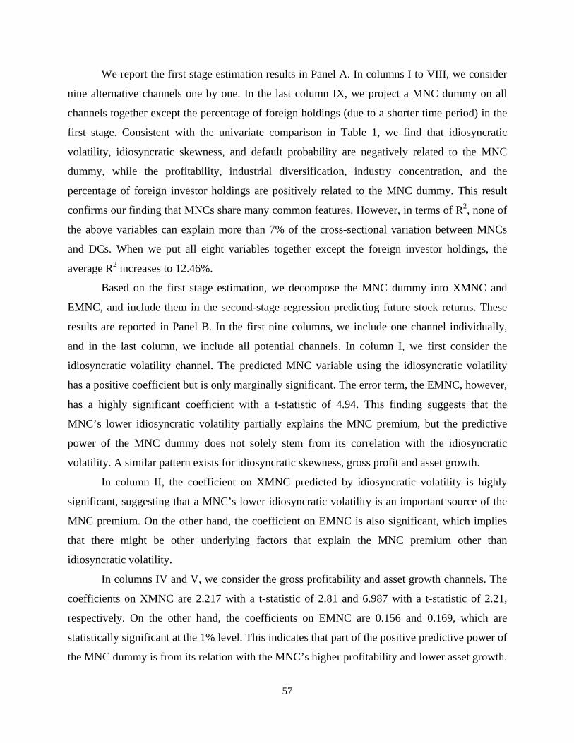
57

We report the first stage estimation results in Panel A. In columns I to VIII, we consider

nine alternative channels one by one. In the last column IX, we project a MNC dummy on all

channels together except the percentage of foreign holdings (due to a shorter time period) in the

first stage. Consistent with the univariate comparison in Table 1, we find that idiosyncratic

volatility, idiosyncratic skewness, and default probability are negatively related to the MNC

dummy, while the profitability, industrial diversification, industry concentration, and the

percentage of foreign investor holdings are positively related to the MNC dummy. This result

confirms our finding that MNCs share many common features. However, in terms of R2, none of

the above variables can explain more than 7% of the cross-sectional variation between MNCs

and DCs. When we put all eight variables together except the foreign investor holdings, the

average R2 increases to 12.46%.

Based on the first stage estimation, we decompose the MNC dummy into XMNC and

EMNC, and include them in the second-stage regression predicting future stock returns. These

results are reported in Panel B. In the first nine columns, we include one channel individually,

and in the last column, we include all potential channels. In column I, we first consider the

idiosyncratic volatility channel. The predicted MNC variable using the idiosyncratic volatility

has a positive coefficient but is only marginally significant. The error term, the EMNC, however,

has a highly significant coefficient with a t-statistic of 4.94. This finding suggests that the

MNC’s lower idiosyncratic volatility partially explains the MNC premium, but the predictive

power of the MNC dummy does not solely stem from its correlation with the idiosyncratic

volatility. A similar pattern exists for idiosyncratic skewness, gross profit and asset growth.

In column II, the coefficient on XMNC predicted by idiosyncratic volatility is highly

significant, suggesting that a MNC’s lower idiosyncratic volatility is an important source of the

MNC premium. On the other hand, the coefficient on EMNC is also significant, which implies

that there might be other underlying factors that explain the MNC premium other than

idiosyncratic volatility.

In columns IV and V, we consider the gross profitability and asset growth channels. The

coefficients on XMNC are 2.217 with a t-statistic of 2.81 and 6.987 with a t-statistic of 2.21,

respectively. On the other hand, the coefficients on EMNC are 0.156 and 0.169, which are

statistically significant at the 1% level. This indicates that part of the positive predictive power of

the MNC dummy is from its relation with the MNC’s higher profitability and lower asset growth.

58

However, the significance of the coefficient on EMNC implies that both of them are not the only

channels that affect the predictive power of a firm’s status as a MNC.

In the last regression, we include all potential channels except the percentage of foreign

holding. We find that both the XMNC and EMNC are positive and significant and the magnitude

of the coefficient on EMNC decreases to 0.101. The result in column X implies that the potential

channels we considered above partially explain why MNCs have higher future returns than DCs,

but many other factors are still not accounted for.

Overall, we examine nine alternative explanations for the MNC return premiums, and

none of the explanations can fully explain the MNC return premium.

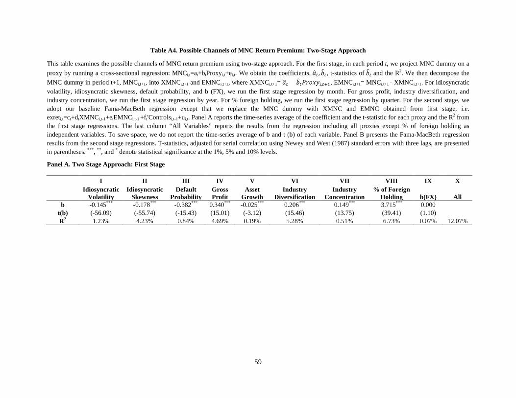
59

Table A4. Possible Channels of MNC Return Premium: Two-Stage Approach

This table examines the possible channels of MNC return premium using two-stage approach. For the first stage, in each period t, we project MNC dummy on a proxy by running a cross-sectional regression: MNCi,t=at+btProxyi,t+ei,t. We obtain the coefficients, 𝑎𝑎�𝑡𝑡 , 𝑏𝑏�𝑡𝑡, t-statistics of 𝑏𝑏�𝑡𝑡 and the R2. We then decompose the MNC dummy in period t+1, MNCi,t+1, into XMNCi,t+1 and EMNCi,t+1, where XMNCi,t+1= 𝑎𝑎�𝑡𝑡 + 𝑏𝑏�𝑡𝑡𝑃𝑃𝑟𝑟𝑐𝑐𝑝𝑝𝐶𝐶𝑖𝑖,𝑡𝑡+1, EMNCi,t+1= MNCi,t+1 - XMNCi,t+1. For idiosyncratic volatility, idiosyncratic skewness, default probability, and b (FX), we run the first stage regression by month. For gross profit, industry diversification, and industry concentration, we run the first stage regression by year. For % foreign holding, we run the first stage regression by quarter. For the second stage, we adopt our baseline Fama-MacBeth regression except that we replace the MNC dummy with XMNC and EMNC obtained from first stage, i.e. exreti,t=ct+dtXMNCi,t-1+etEMNCi,t-1 +ft'Controlsi,t-1+ui,t. Panel A reports the time-series average of the coefficient and the t-statistic for each proxy and the R2 from the first stage regressions. The last column “All Variables” reports the results from the regression including all proxies except % of foreign holding as independent variables. To save space, we do not report the time-series average of b and t (b) of each variable. Panel B presents the Fama-MacBeth regression results from the second stage regressions. T-statistics, adjusted for serial correlation using Newey and West (1987) standard errors with three lags, are presented in parentheses. ***, **, and * denote statistical significance at the 1%, 5% and 10% levels.

Panel A. Two Stage Approach: First Stage

I II III IV V VI VII VIII IX X

Idiosyncratic

Volatility Idiosyncratic

Skewness Default

Probability Gross Profit

Asset Growth

Industry Diversification

Industry Concentration

% of Foreign Holding b(FX) All

b -0.145*** -0.178*** -0.382*** 0.340*** -0.025*** 0.206*** 0.149*** 3.715*** 0.000 t(b) (-56.09) (-55.74) (-15.43) (15.01) (-3.12) (15.46) (13.75) (39.41) (1.10) R2 1.23% 4.23% 0.84% 4.69% 0.19% 5.28% 0.51% 6.73% 0.07% 12.07%

60

Panel B. Two Stage Approach: Second Stage

I II III IV V VI VII VIII IX X

Idio.

Volatility Idio.

Skewness Default

Probability Gross Profit

Asset Growth

Industry Div.

Industry Con.

% of Foreign Holding b(FX) All

Intercept -0.977 -1.241 -3.355 -0.218 -1.251 0.609 0.720 0.620 -5.213 -0.283

(-0.82) (-1.07) (-1.28) (-0.39) (-1.02) (1.14) (1.24) (1.02) (-0.70) (-0.53) XMNC 5.347* 6.917*** 12.670 2.217*** 6.987** 0.104 -0.150 0.404 15.995 1.703***

(1.87) (2.88) (1.58) (2.81) (2.12) (0.17) (-0.19) (1.19) (0.79) (7.20) EMNC 0.225*** 0.233*** 0.277*** 0.156*** 0.169*** 0.209*** 0.228*** 0.213** 0.226*** 0.101*

(4.94) (4.92) (5.13) (3.54) (3.92) (4.68) (4.94) (2.30) (5.02) (1.68) Ln(Size) -0.150*** -0.218*** -0.083** -0.093** -0.094** -0.101*** -0.110*** -0.095** -0.103*** -0.124***

(-4.68) (-5.74) (-2.23) (-2.44) (-2.56) (-2.70) (-2.87) (-2.05) (-2.75) (-3.36) B/M 0.622*** 0.664*** 0.653*** 0.683*** 0.583*** 0.627*** 0.616*** 0.460*** 0.630*** 0.626***

(9.49) (9.56) (9.57) (9.96) (8.53) (9.30) (8.99) (3.83) (9.32) (8.53) Prev. 6-Month Ret. 0.005*** 0.006*** 0.008*** 0.005*** 0.005*** 0.006*** 0.005*** 0.001 0.005*** 0.008***

(3.89) (3.89) (5.59) (4.06) (3.53) (4.21) (3.75) (0.27) (4.07) (5.14) b(MKT) -0.015 -0.053 -0.042 -0.046 -0.039 -0.055 -0.047 -0.109 -0.051 -0.032

(-0.34) (-0.99) (-0.76) (-0.94) (-0.79) (-1.11) (-0.92) (-0.98) (-1.04) (-0.56) b(SMB) -0.079*** -0.083*** -0.056** -0.078*** -0.083*** -0.079*** -0.084*** -0.080** -0.081*** -0.073***

(-3.74) (-3.80) (-2.37) (-3.55) (-3.75) (-3.59) (-3.70) (-2.03) (-3.63) (-3.05) b(HML) 0.004 0.012 0.007 0.011 0.006 0.014 0.012 -0.027 0.013 0.003

(0.18) (0.48) (0.29) (0.49) (0.28) (0.60) (0.50) (-0.59) (0.57) (0.11) b(FX) 0.006 0.010 0.007 0.005 0.004 0.008 0.006 0.005 0.002 -0.002

(0.59) (0.88) (0.60) (0.41) (0.37) (0.74) (0.48) (0.20) (0.82) (-0.16) Industry Dummies Y Y Y Y Y Y Y Y Y Y Start Date 197302 197302 197302 197302 197302 197302 197307 200007 197302 197307 End Date 201512 201201 201101 201512 201512 201512 201512 201512 201512 201101 Adjusted R2 5.90% 6.50% 6.80% 5.70% 5.90% 5.60% 5.40% 6.40% 5.50% 7.00%

61

A5. MNC Return Premium by Industry

Similar to the size dimension approach, we re-estimate the Fama-MacBeth regression in

equation (1) within each industry, allowing the coefficients to vary across industries, using

Fama-French 30 industry classifications.17 In Table A4, we first present the number of firms and

the percentage of MNCs within each industry. “Chemicals”, “Fabricated Products and

Machinery” and “Automobiles and Trucks” are the top three industries with the highest MNC

percentage around 65%, while “Utilities”, “Banking”, and “Retail” are the bottom three with the

MNC percentage under 20%. In the next two columns, we find that the coefficients for the MNC

dummy are positive for all but eight industries, varying between 0.036 and 0.468, indicating that

the MNC premium is not restricted to a subset of industries. For eight industries, the coefficient

is positive and statistically significant at 10% or lower. In particular, the “Chemicals” industry

has the largest coefficient, 0.468, on the MNC dummy of 0.468, followed by “Automobiles and

Trucks” and “Personal and Business Services”.

To further understand whether the different magnitude of MNC premium across

industries depends on the types of the products and services that firms produce, following Mian

and Sufi (2014), we categorize industries into tradable and non-tradable industries using the 4-

digit NAICS industry codes. While tradable industries are involved in intensive imports and

exports of goods, non-tradable industries including retail, food service, and construction produce

services that are not easily traded. At the bottom of the Table A4, we find that the MNC

coefficient of tradable industries is positive and highly significant, while the coefficient is

marginally significant for non-tradable industries. The results of higher returns for MNCs in

tradable industries are consistent with the hypothesis that MNCs are exposed to additional

foreign operational risks that domestic firms do not have to bear, resulting in higher returns.

17 To obtain relatively reliable estimates, we require each industry to have at least 20 firms each month, resulting in three industries dropped from the sample (Beer and Liquor, Tobacco Products, and Coal).

62

Table A5. MNC Return Premium by Industry: U.S. Sample

This table reports the Fama-MacBeth regression results by industry for the U.S. sample. The sample period is from February 1973 to December 2015. This table presents the average number of firms, and the average percentage of MNCs, the coefficients and t-stats of the MNC dummy by industry based on the Fama-French 30 industry classification. The results are sorted in descending order based on the size of the coefficient on MNC dummy. Industries with less than 20 firms are omitted. Tradable and non-tradable industries are based on Mian and Sufi (2014). T-statistics, adjusted for serial correlation using Newey and West (1987) standard errors with three lags, are presented in parentheses. ***, **, and * denote statistical significance at the 1%, 5% and 10% levels.

FF 30 Industry Description # of

Firms % of MNC

MNC Dummy t-stat

9 Chemicals 77 68.39% 0.468** (2.18) 15 Automobiles and Trucks 59 64.24% 0.456* (1.65) 22 Personal and Business Services 408 42.72% 0.443*** (3.95) 21 Communication 79 22.84% 0.441** (2.28) 8 Healthcare, Medical Equipment, Pharmaceutical Products 316 34.62% 0.421*** (2.80)

16 Aircraft, Ships, and Railroad Equipment 30 48.53% 0.391* (1.65) 13 Fabricated Products and Machinery 157 65.97% 0.374** (2.36) 23 Business Equipment 411 56.16% 0.329*** (2.83) 14 Electrical Equipment 94 50.40% 0.224 (1.15) 10 Textiles 33 45.64% 0.213 (0.77) 29 Banking, Insurance, Real Estate, Trading 642 9.24% 0.203 (1.52) 30 Others 98 37.29% 0.190 (1.06) 1 Food Products 95 39.41% 0.175 (1.19) 4 Recreation 86 39.09% 0.155 (0.82)

19 Petroleum and Natural Gas 163 34.89% 0.113 (0.85) 11 Construction and Construction Materials 159 39.51% 0.101 (0.74) 24 Business Supplies and Shipping Containers 66 55.59% 0.097 (0.62) 27 Retail 209 18.96% 0.069 (0.50) 6 Consumer Goods 85 53.83% 0.036 (0.19)

20 Utilities 151 3.57% -0.032 (-0.13) 7 Apparel 57 45.99% -0.075 (-0.35)

26 Wholesale 160 35.37% -0.079 (-0.68) 5 Printing and Publishing 59 39.25% -0.099 (-0.55)

17 Precious Metals, Non-Metallic, and Industrial Metal Mining 36 36.33% -0.100 (-0.36) 25 Transportation 89 28.76% -0.105 (-0.70) 28 Restaurants, Hotels, Motels 85 20.72% -0.138 (-0.74) 12 Steel Works 61 47.36% -0.157 (-0.98)

Tradable Industries 1,988 53.93% 0.372*** (4.77)

Non-tradable Industries 2,050 22.41% 0.139* (1.77)