Embed Size (px)
Citation preview
The Maxima Book
Paulo Ney de SouzaRichard J. Fateman
Joel MosesCliff Yapp
19th March 2003

1
Credits
Paulo Ney de SouzaJay BelangerRichard FatemanJoel MosesCliff Yapp
Contents
Preface 5
I The Maxima Program and Standard Packages 6
1 Introduction 71.1 What is Maxima?. . . . . . . . . . . . . . . . . . . . . . . . . . . . . . . . . . . . . . . . . . . . . 71.2 A Brief History of Macsyma. . . . . . . . . . . . . . . . . . . . . . . . . . . . . . . . . . . . . . . 8
2 Installing 102.1 Installing on Linux . . . . . . . . . . . . . . . . . . . . . . . . . . . . . . . . . . . . . . . . . . . .10
2.1.1 The Easy Way . . . . . . . . . . . . . . . . . . . . . . . . . . . . . . . . . . . . . . . . . .102.1.2 The Hard Way . . . . . . . . . . . . . . . . . . . . . . . . . . . . . . . . . . . . . . . . . .10
2.2 Installing on Windows . . . . . . . . . . . . . . . . . . . . . . . . . . . . . . . . . . . . . . . . . .122.2.1 The Easy Way - Installing the Windows Binary. . . . . . . . . . . . . . . . . . . . . . . . . 122.2.2 The Hard Way . . . . . . . . . . . . . . . . . . . . . . . . . . . . . . . . . . . . . . . . . .12
3 Available Interfaces to Maxima 133.1 The Terminal Interface. . . . . . . . . . . . . . . . . . . . . . . . . . . . . . . . . . . . . . . . . .133.2 The Emacs Interface. . . . . . . . . . . . . . . . . . . . . . . . . . . . . . . . . . . . . . . . . . .14
3.2.1 Installing the Maxima Emacs Mode. . . . . . . . . . . . . . . . . . . . . . . . . . . . . . . 143.2.2 Maxima-mode . . . . . . . . . . . . . . . . . . . . . . . . . . . . . . . . . . . . . . . . . .153.2.3 Enhanced Terminal Mode. . . . . . . . . . . . . . . . . . . . . . . . . . . . . . . . . . . . 173.2.4 Emaxima Mode. . . . . . . . . . . . . . . . . . . . . . . . . . . . . . . . . . . . . . . . . .17
3.3 Xmaxima . . . . . . . . . . . . . . . . . . . . . . . . . . . . . . . . . . . . . . . . . . . . . . . . .283.4 Symaxx . . . . . . . . . . . . . . . . . . . . . . . . . . . . . . . . . . . . . . . . . . . . . . . . . .303.5 TEXmacs . . . . . . . . . . . . . . . . . . . . . . . . . . . . . . . . . . . . . . . . . . . . . . . . .32
4 The Basics - What you need to know to operate in Maxima 344.1 The Very Beginning. . . . . . . . . . . . . . . . . . . . . . . . . . . . . . . . . . . . . . . . . . . .34
4.1.1 Our first Maxima Session. . . . . . . . . . . . . . . . . . . . . . . . . . . . . . . . . . . . 344.1.2 To Evaluate or Not to Evaluate. . . . . . . . . . . . . . . . . . . . . . . . . . . . . . . . . . 384.1.3 The Concept of Environment - Theev Command. . . . . . . . . . . . . . . . . . . . . . . . 384.1.4 Clearing values from the system - thekill command. . . . . . . . . . . . . . . . . . . . . . 43
4.2 Common Operators in Maxima. . . . . . . . . . . . . . . . . . . . . . . . . . . . . . . . . . . . . . 434.2.1 Assignment Operators. . . . . . . . . . . . . . . . . . . . . . . . . . . . . . . . . . . . . . 43
5 Trig through Calculus 475.1 Trigonometric Functions. . . . . . . . . . . . . . . . . . . . . . . . . . . . . . . . . . . . . . . . .475.2 Differentiation. . . . . . . . . . . . . . . . . . . . . . . . . . . . . . . . . . . . . . . . . . . . . . .485.3 Integration. . . . . . . . . . . . . . . . . . . . . . . . . . . . . . . . . . . . . . . . . . . . . . . . .50
2
CONTENTS 3
5.3.1 Theassume Command. . . . . . . . . . . . . . . . . . . . . . . . . . . . . . . . . . . . . . 515.3.2 Definite Integrals. . . . . . . . . . . . . . . . . . . . . . . . . . . . . . . . . . . . . . . . .525.3.3 changevar . . . . . . . . . . . . . . . . . . . . . . . . . . . . . . . . . . . . . . . . . . . .535.3.4 Behind the Black Box - Using Specific Approaches. . . . . . . . . . . . . . . . . . . . . . . 535.3.5 Other Examples. . . . . . . . . . . . . . . . . . . . . . . . . . . . . . . . . . . . . . . . . .53
6 Advanced Mathematics - ODEs and Beyond 556.1 Ordinary Differential Equations. . . . . . . . . . . . . . . . . . . . . . . . . . . . . . . . . . . . . 55
6.1.1 Defining Ordinary Differential Equations. . . . . . . . . . . . . . . . . . . . . . . . . . . . 556.1.2 Solving Ordinary Differential Equations:ode2 . . . . . . . . . . . . . . . . . . . . . . . . . 566.1.3 Solving Ordinary Differential Equations:desolve . . . . . . . . . . . . . . . . . . . . . . . 62
7 Matrix Operations and Vectors 65
8 Introduction to Maxima’s Programming Language 668.1 Some Examples. . . . . . . . . . . . . . . . . . . . . . . . . . . . . . . . . . . . . . . . . . . . . .668.2 Unconventional Conditionals. . . . . . . . . . . . . . . . . . . . . . . . . . . . . . . . . . . . . . . 678.3 Assumptions . . . . . . . . . . . . . . . . . . . . . . . . . . . . . . . . . . . . . . . . . . . . . . .678.4 Arbitrary Numbers of Parameters. . . . . . . . . . . . . . . . . . . . . . . . . . . . . . . . . . . . . 688.5 Arrays . . . . . . . . . . . . . . . . . . . . . . . . . . . . . . . . . . . . . . . . . . . . . . . . . . .688.6 Iteration . . . . . . . . . . . . . . . . . . . . . . . . . . . . . . . . . . . . . . . . . . . . . . . . . .698.7 Serious Business. . . . . . . . . . . . . . . . . . . . . . . . . . . . . . . . . . . . . . . . . . . . .698.8 Hardcopy . . . . . . . . . . . . . . . . . . . . . . . . . . . . . . . . . . . . . . . . . . . . . . . . .708.9 Return to Arrays and Functions. . . . . . . . . . . . . . . . . . . . . . . . . . . . . . . . . . . . . . 708.10 More Useful Examples. . . . . . . . . . . . . . . . . . . . . . . . . . . . . . . . . . . . . . . . . .708.11 Part Hacking . . . . . . . . . . . . . . . . . . . . . . . . . . . . . . . . . . . . . . . . . . . . . . .728.12 User Representation of Data. . . . . . . . . . . . . . . . . . . . . . . . . . . . . . . . . . . . . . . 73
9 Graphics and Forms of Output 759.1 Options on the Command Line. . . . . . . . . . . . . . . . . . . . . . . . . . . . . . . . . . . . . . 75
9.1.1 1D vs. 2D. . . . . . . . . . . . . . . . . . . . . . . . . . . . . . . . . . . . . . . . . . . . .759.1.2 TeX Strings as Output. . . . . . . . . . . . . . . . . . . . . . . . . . . . . . . . . . . . . . 759.1.3 Writing a Session to a File. . . . . . . . . . . . . . . . . . . . . . . . . . . . . . . . . . . . 76
9.2 Graphics. . . . . . . . . . . . . . . . . . . . . . . . . . . . . . . . . . . . . . . . . . . . . . . . . .789.2.1 2D function plotting . . . . . . . . . . . . . . . . . . . . . . . . . . . . . . . . . . . . . . . 789.2.2 3D Function Plotting. . . . . . . . . . . . . . . . . . . . . . . . . . . . . . . . . . . . . . . 78
9.3 Plot Options. . . . . . . . . . . . . . . . . . . . . . . . . . . . . . . . . . . . . . . . . . . . . . . .79
10 Maxims for the Maxima User 84
11 Help Systems and Debugging 86
12 Troubleshooting 87
13 Advanced Examples 88
II External, Additional, and Contributed Packages 91
14 The Concept of Packages - Expanding Maxima’s Abilities 92
15 Available Packages for Maxima 93
List of Figures 93
Index 94

CONTENTS 4
Bibliography 96
CONTENTS 5
Many hands and minds have contributed to Macsyma, in developing it as a research program, and tuning it for useby others. We have enjoyed constructing Macsyma and we hope that you will enjoy using it. We hope you will considercontributing your carefully polished and documented application programs to libraries at your local installation andother sites.
Examples
1. First Example 342. Quitting Maxima 353. End of Entry Characters 364. Line Labels 365. Labeling an Example Equation 37
6. Evaluation Toggle 387. Basic Use of ev Command 388. ev’s Expand Option 399. Float Example ??

Part I
The Maxima Program and StandardPackages
6
CHAPTER 1
Introduction
1.1 What is Maxima?
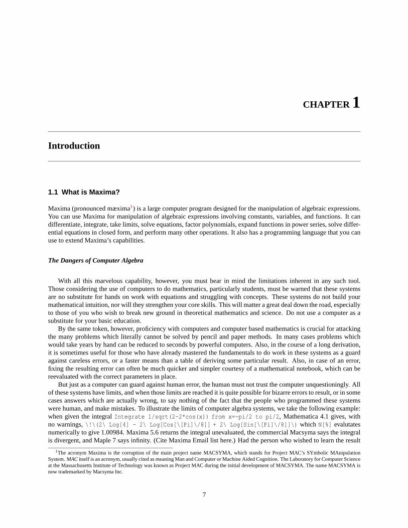
Maxima (pronounced mæxime1) is a large computer program designed for the manipulation of algebraic expressions.You can use Maxima for manipulation of algebraic expressions involving constants, variables, and functions. It candifferentiate, integrate, take limits, solve equations, factor polynomials, expand functions in power series, solve differ-ential equations in closed form, and perform many other operations. It also has a programming language that you canuse to extend Maxima’s capabilities.
The Dangers of Computer Algebra
With all this marvelous capability, however, you must bear in mind the limitations inherent in any such tool.Those considering the use of computers to do mathematics, particularly students, must be warned that these systemsare no substitute for hands on work with equations and struggling with concepts. These systems do not build yourmathematical intuition, nor will they strengthen your core skills. This will matter a great deal down the road, especiallyto those of you who wish to break new ground in theoretical mathematics and science. Do not use a computer as asubstitute for your basic education.
By the same token, however, proficiency with computers and computer based mathematics is crucial for attackingthe many problems which literally cannot be solved by pencil and paper methods. In many cases problems whichwould take years by hand can be reduced to seconds by powerful computers. Also, in the course of a long derivation,it is sometimes useful for those who have already mastered the fundamentals to do work in these systems as a guardagainst careless errors, or a faster means than a table of deriving some particular result. Also, in case of an error,fixing the resulting error can often be much quicker and simpler courtesy of a mathematical notebook, which can bereevaluated with the correct parameters in place.
But just as a computer can guard against human error, the human must not trust the computer unquestioningly. Allof these systems have limits, and when those limits are reached it is quite possible for bizarre errors to result, or in somecases answers which are actually wrong, to say nothing of the fact that the people who programmed these systemswere human, and make mistakes. To illustrate the limits of computer algebra systems, we take the following example:when given the integralIntegrate 1/sqrt(2-2*cos(x)) from x=-pi/2 to pi/2, Mathematica 4.1 gives, withno warnings,\!\(2\ Log[4] - 2\ Log[Cos[\[Pi]\/8]] + 2\ Log[Sin[\[Pi]\/8]]\) which N[%] evalutatesnumerically to give 1.00984. Maxima 5.6 returns the integral unevaluated, the commercial Macsyma says the integralis divergent, and Maple 7 says infinity. (Cite Maxima Email list here.) Had the person who wished to learn the result
1The acronym Maxima is the corruption of the main project name MACSYMA, which stands for Project MAC’s SYmbolic MAnipulationSystem.MAC itself is an acronym, usually cited as meaning Man and Computer or Machine Aided Cognition. The Laboratory for Computer Scienceat the Massachusetts Institute of Technology was known as Project MAC during the initial development of MACSYMA. The name MACSYMA isnow trademarked by Macsyma Inc.
7
CHAPTER 1. INTRODUCTION 8
blindly trusted most of the systems in question, he might have been misled. So remember to think about the resultsyou are given. The computer is not always necessarily right, and even if it gives a correct answer that answer is notnecessarily complete.
1.2 A Brief History of Macsyma
The birthplace of Macsyma, where much of the original coding took place, was Project MAC at MIT in the late 1960sand earlier 1970s. Project MAC was an MIT research unit, which was folded into the current Laboratory for ComputerScience. Research support for Macsyma included the Advanced Research Projects Agency(ARPA), Department ofDefense, the US Department of Energy, and other government and private sources.
The original idea, first voiced by Marvin Minsky, was to automate the kinds of manipulations done by mathe-maticians, as a step toward understanding the power of computers to exhibit a kind of intelligent behavior. [Pro63]The undertaking grew out of a previous effort at MITRE Corp called Mathlab, work of Carl Engelman and others,plus the MIT thesis work of Joel Moses on symbolic integration, and the MIT thesis work of William A. Martin. Thenew effort was dubbed Macsyma - Project MAC’s SYmbolic MAnipulator. The original core design was done in July1968, and coding began in July 1969. This was long before the days of personal computers and cheap memory - initialdevelopment was centered around a single computer shared with the Artificial Intelligence laboratory, a DEC PDP-6.This was replaced by newer more powerful machines over the years, and eventually the Mathlab group acquired itsown DEC-PDP-10, MIT-ML running the ITS operating system. This machine became a host on the early ARPANET,predecessor to the internet, which helped it gain a wider audience. As the effort grew in scope and ability the generalinterest it created led to attempts to "port" the code - that is, to take the series of instructions which had been writtenfor one machine and operating system and adapt them to run on another, different system. The earliest such effort wasthe running of Macsyma in a MacLisp environment on a GE/Honeywell Multics mainframe, another system at MIT.The Multics environment provided essentially unlimited address space, but for various reasons the system was notfavored by programmers and the Multics implementation was never popular. The next effort came about when a groupat MIT designed and implemented a machine which was based on the notion that hardware support of Lisp wouldmake it possible to overcome problems that inhibited the solution of many interesting problems. The Lisp machineclearly had to support Macsyma, the largest Lisp program of the day, and the effort paid off with probably the bestenvironment for Macsyma to date (although requiring something of an expert perspective). Lisp machines, as wellas other special purpose hardware, tended to become slow and expensive compared to off-the-shelf machines builtaround merchant-semiconductor CPUs, and so the two companies that were spun off from MIT (Symbolics Inc, andLMI) both eventually disappeared. Texas Instruments built a machine called the Explorer bases on the LMI design,but also stopped production.
Around 1980, the idea of porting Macsyma began to be more interesting, and the Unix based vaxima distribution,which ran on a Lisp system built at the University of California at Berkeley for VAX UNIX demonstrated that it wasboth possible and practical to run the software on less expensive systems. (This system, Franz Lisp, was implementedprimarily in Lisp with some parts written in C.) Once the code stabilized, the new version opened up porting possibili-ties, ultimately producing at least six variations on the theme which included Macsyma, Maxima, Paramax/Paramacs,Punimax, Aljbar, and Vaxima. These have followed somewhat different paths, and most were destined to fade into thesunset. The two which survived obscurity, Maxima and Macsyma, we will discuss below. Punimax was actually anoffshoot of Maxima - some time around 1994 Bruno Haible (author of clisp) ported maxima to clisp. Due to the legalconcerns of Richard Petti, then the owner of the commercial Macsyma, the name was changed to Punimax. It has notseen much activity since the initial port, and although it is still available the ability of the main Maxima distribution tocompile on Clisp makes further development of Punimax unlikely.
There is a certain surprising aspect in this multiplicity of versions and platforms, given how the code seemed tiedto the development environment, which included a unique operating system. Fortunately, Berkeley’s building a replicaof the Maclisp environment on the MIT-ML PDP-10, using tools available in almost any UNIX/C environment, helpedsolve this problem. Complicating the matter was the eventual demise of the PDP-10 and Maclisp systems as CommonLisp (resembling lisp-machine lisp), influenced by BBN lisp and researchers at Stanford, Carnegie Mellon University,and Xerox, began to take hold. It seemed sensible to re-target the code to make it compatible with what eventuallybecame the ANSI Common Lisp standard. Since almost everything needed for for Macsyma can be done in ANSICL, the trend toward standardization made many things simpler. There are a few places where the language is notstandardized, in particular connecting to modules written in other languages, but much of the power of the system canbe expressed within ANSI CL. It is a trend the Maxima project is planning to carry on, to maintain and expand on this
CHAPTER 1. INTRODUCTION 9
flexibility which has emerged.With all these versions, in recent history there are two which have been major players, due this time more to
economics than to code quality. 1982 was a watershed year in many respects for Macsyma - it marks clearly thebranching of Macsyma into two distinct products, and ultimately gave rise to the events which have made Maximaboth possible and desirable. MIT had decided, with the gradual spread of computers throughout the academic world, toput Macsyma on the market commercially, using as a marketing partner the firm of Arthur D. Little, Inc. This versionwas sold to the Symbolics Inc., which, depending on your perspective, either turned the project into a significantmarketing effort to help sell their high-priced lisp machines, or was a diversionary tactic to deny their competitors(LMI) this program. At the same time MIT forced UC Berkeley (Richard Fateman) to withdraw the copies fromabout 50 sites of the VAX/UNIX and VAX/VMS versions of Macsyma that he had distributed with MIT’s consent,until some agreement could be reached for technology transfer. Symbolics hired some of the MIT staff to work atSymbolics in order to improve the code,which was now proprietary. The MIT-ML PDP-10 also went off the Arpanetin 1983. (Interestingly, the closing of the MIT Lisp and Macsyma efforts was a key reason Richard Stallman decidedto form the Free Software Foundation.) Between the high prices, closed source code, and neglecting all platforms infavor of Lisp Machines pressure came to bear on MIT to release another version to accommodate these needs, whichthey did with some reluctance. The new version was distributed via the National Energy Software Center, and calledDOE Macsyma. It had been re-coded in a dialect of lisp written for the VAX at MIT called NIL. There was never acomplete implementation. At about the same time a VAX/UNIX version "VAXIMA" was put into the same libraryby Berkeley. This ran on any of hundreds of machines running the Berkeley version of VAX Unix, and through aUNIX simulator on VMS, on any VAX system. The DOE versions formed the basis of the subsequent non-Symbolicsdistributions. The code was made available through the National Energy Software Center, which in its attempt torecoup its costs, charged a significant fee($1-2k?). It provided full source, but in a concession to MIT, did not allowredistribution. This prohibition seems to have been disregarded, and especially so since NESC disappeared. Perhapsit didn’t recoup its costs! Among all the new activity centered around DOE Macsyma, Prof. William Schelter beganmaintaining a version of the code at UT Austin, calling his variation Maxima. He refreshed the NESC version with acommon-lisp compatible code version.
There were, from the earliest days, other computer algebra systems including Reduce, CAMAL, Mathlab-68, PM,and ALTRAN. More serious competition, however, did not arrive until Maple and Mathematica were released, Maplein 1985 (Cite list of dates) and Mathematica in 1988 (cite wolfram website). These systems were inspired by Macsymain terms of their capabilities, but they proved to be much better at the challenge of building mind-share. DOE-Macsyma, because of the nature of its users and maintainers, never responded to this challenge. Symbolics’ successorMacsyma Inc, having lost market share and unable to meet its expenses, was sold in the summer of 1999 after attemptsto find endowment and academic buyers failed. (Cite Richard Petti usenet post.) The purchaser withdrew Macsymafrom the market and the developers and maintainers of that system dispersed. Mathematica and Maple appeared tohave vanquished Macsyma.
It was at this point Maxima re-entered the game. Although it was not widely known in the general academic public,W. Schelter had been maintaining and extending his copy of the code ever since 1982. He had decided to see whathe could do about distributing it more widely. He attempted to contact the NESC to request permission to distributederivative works. The duties of the NESC had been assumed in 1991 by the Energy Science and Technology SoftwareCenter, which granted him virtually unlimited license to make and distribute derivative works, with some minor exportrelated caveats.
It was a significant breakthrough. While Schelter’s code had been available for downloading for years, this activitybecame legal with the release from DOE granted in Oct. 1998, and Maxima began to attract more attention. Whenthe Macsyma company abruptly vanished in 1999, with no warning or explanation, it left their customer base hanging.They began looking for a solution, and some drifted toward Maxima.
Dr. Schelter maintained the Maxima system until his untimely death in July, 2001. It was a hard and unexpectedblow, but Schelter’s obtaining the go-ahead to release the source code saved the project and possibly even the Macsymasystem itself. A group of users and developers who had been brought together by the email list for Maxima decided totry and form a working open source project around the Maxima system, rather than let it fade - which is where we aretoday.
CHAPTER 2
Installing
2.1 Installing on Linux
Note: This is written for version 5.6. With 5.9 things should change significantly, both for Windows and Linux, so arewrite will be performed at that time.
2.1.1. The Easy Way
If you are using Debian Linux, there are packages for Maxima in the Debian archives. Redhat users can find packagesat rpmfind.net and mirrors. To the best of my knowledge these packages are all compiled against GNU Common Lisp(GCL). GCL does not access the readline library, which makes using Maxima on the terminal somewhat cumbersome.There are various interfaces which address this issue, but in the case of these packages the left arrow key will not takeyou back to the middle of an expression and let you edit just what you want - you will have to delete everything backto the point where you made your error. See the interfaces section for more about this, or if you really want to usemaxima in the terminal I’d recommend compiling against CLISP.
2.1.2. The Hard Way
Compiling Maxima on Linux should go reasonably smoothly, although some distributions seem to have problems withthe makefiles. Redhat 7.1 is known to be a bit flaky in this regard.
Compiling with GCL
GCL is the version of Lisp Maxima has been maintained on for many years by William Schelter, and thus the defaultsystem on which to build Maxima. Maxima will typically be made to work with GCL, and then be fixed to work withother Lisps. If in doubt, start here, but again be warned that readline support is not present in GCL.
The first step in this process is to compile GCL. The files from the compiling of GCL are needed when buildingMaxima against it, so first download and decompress the most current version of GCL. Compiling it should be simple:
cd $HOME/gcl./configuremake
Once that is complete, download and decompress Maxima. Now the process gets a little more complicated - youwill have to hand edit the fileconfigure. What follows is the first part of the file, with the parts you must edit in bold:
#!/bin/sh
10
CHAPTER 2. INSTALLING 11
# edit next few lines# GCLDIR should be where gcl was built, and the o/*.o lsp/*.o etc must be# there to link with maximaGCLDIR=/home/cliff/gcl-2.3.8# the directory where this file is, and where you will build maxima# could useMAXDIR= /home/cliff/maxima-5.5MAXDIR=‘pwd‘# where to put some maxima .el filesEMACS_SITE_LISP=/usr/lib/emacs/site-lisp# determines where to install# PREFIX_DIR=/usr/local puts things in /usr/local/lib/maxima-x.y# and /usr/local/binPREFIX_DIR=/usr/localINFO_DIR=${PREFIX_DIR}/infoMAN_DIR=${PREFIX_DIR}/man/man1##### end editing #########
Once this is correctly done, run the configure script:./configure. If this succeeds without any problems, runmake. This could be a long process, depending on your machine. Once it is done, and if no errors result, runmaketest. If any errors appear in either stage, consult the trouble shooting section. Otherwise, you are ready to su into rootand runmake install. Once this process is completed, you should be able to runmaxima andxmaxima. Emacs modemay take a little more work, and the other interfaces are separate programs - see the Interfaces chapter for details.
Compiling with CLISP
Clisp has, among other features, the ability to use the readline library. This means that many of the limitations createdin the terminal by GCL are not relevant here, and for the beginner especially this is a good place to start. Unfortunately,compiling on a flavor of Lisp other than GCL is not quite as smooth - here are the steps.
Change into the directory $HOME/maxima/src (or $HOME/maxima-5.6/src - whatever your setup dictates.)For newer versions of clisp, you need to change a couple lines in the file compile-clisp.lisp:
< (lisp:gc)→ (ext:gc)< (lisp:saveinitmem "maxima-clisp.mem"→ (ext:saveinitmem "maxima-clisp.mem"
Then run the following commands:
make clisp-compile CLISP=clispmake maxima-clisp.mem CLISP=clispmake test-clisp CLISP=clisp
Once that is complete, you can either leave maxima where you built it, or move the directory to a more suitableplace. Once that is done, in order to set up a convenient way to run Maxima, you can create some shell scripts in/usr/local/bin (make sure to do chmod +x on both files):
===================maxima==============#!/bin/bashexport MAXIMA_DIRECTORY=/PATH_TO_NEW_DIRECTORY/maximaexec clisp -M ${MAXIMA_DIRECTORY}/src/maxima-clisp.mem=======================================
===============xmaxima==================#!/bin/bash
CHAPTER 2. INSTALLING 12
export MAXIMA_DIRECTORY=/PATH_TO_NEW_DIRECTORY/maximaexec ${MAXIMA_DIRECTORY}/bin/xmaxima -lisp clisp=======================================
Compiling with CMULISP
Other Lisps
2.2 Installing on Windows
2.2.1. The Easy Way - Installing the Windows Binary
This is the recommended way to use Maxima on Windows. The current binary release is technically a beta, but shouldserve most needs quite well. Here is how a basic install works:
1. Download the binary from http://www.ma.utexas.edu/maxima.html It should be named maxima55l-setup.exe
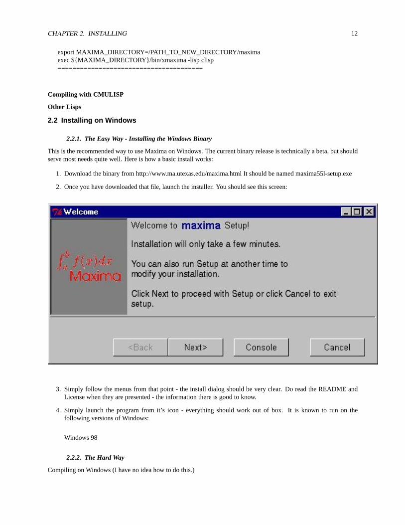
2. Once you have downloaded that file, launch the installer. You should see this screen:
3. Simply follow the menus from that point - the install dialog should be very clear. Do read the README andLicense when they are presented - the information there is good to know.
4. Simply launch the program from it’s icon - everything should work out of box. It is known to run on thefollowing versions of Windows:
Windows 98
2.2.2. The Hard Way
Compiling on Windows (I have no idea how to do this.)
CHAPTER 3
Available Interfaces to Maxima
Maxima is at heart a command line program, and by itself it is not capable of displaying formatted mathematicsbeyond the ascii text level. However there are other interfaces which may be used. Maxima has the ability to exportexpressions using the TEX syntax, and several programs use this device to help with output formatting. (None at thistime allow formatted input.) All have their strengths and weaknesses - the choice will likely depend on the skill ofthe user and the task at hand. We will discuss here all of the interfaces currently available, and the user can make thechoice him/herself which one to use.
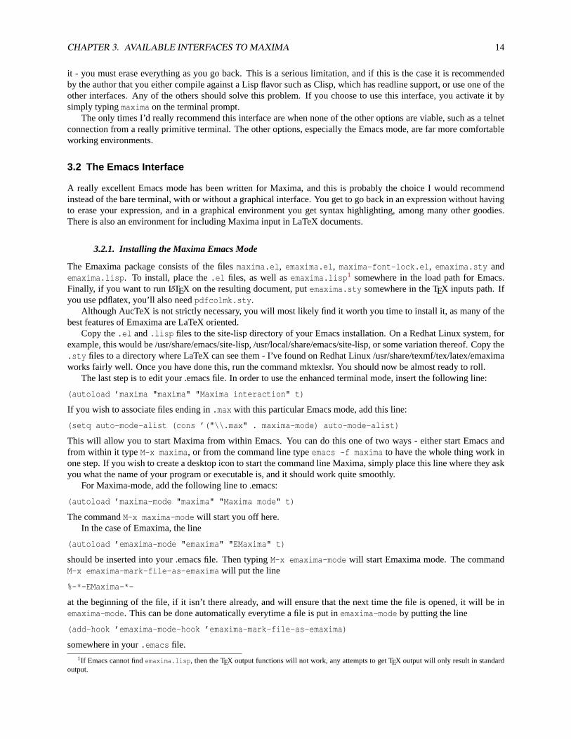
3.1 The Terminal Interface
The terminal interface is the original interface to Maxima. While in some sense all of the interfaces to Maximacould be termed Terminal interfaces, when we refer to it here we mean the command line, no frills interface you woulduse in an xterm or a nongraphical terminal. It is the least capable of all the alternatives in many respects, but it is alsothe least demanding.
How comfortable this interface is depends to a large extent on what Lisp you used to compile Maxima originally.If you used the default, which is gcl, (what all binary packages I am aware of use) you do not have readline support onthe terminal. This means you will not be able to use the back arrow key to go to the middle of an expression and change
13
CHAPTER 3. AVAILABLE INTERFACES TO MAXIMA 14
it - you must erase everything as you go back. This is a serious limitation, and if this is the case it is recommendedby the author that you either compile against a Lisp flavor such as Clisp, which has readline support, or use one of theother interfaces. Any of the others should solve this problem. If you choose to use this interface, you activate it bysimply typingmaxima on the terminal prompt.
The only times I’d really recommend this interface are when none of the other options are viable, such as a telnetconnection from a really primitive terminal. The other options, especially the Emacs mode, are far more comfortableworking environments.
3.2 The Emacs Interface
A really excellent Emacs mode has been written for Maxima, and this is probably the choice I would recommendinstead of the bare terminal, with or without a graphical interface. You get to go back in an expression without havingto erase your expression, and in a graphical environment you get syntax highlighting, among many other goodies.There is also an environment for including Maxima input in LaTeX documents.
3.2.1. Installing the Maxima Emacs Mode
The Emaxima package consists of the filesmaxima.el, emaxima.el, maxima-font-lock.el, emaxima.sty andemaxima.lisp. To install, place the.el files, as well asemaxima.lisp1 somewhere in the load path for Emacs.Finally, if you want to run LATEX on the resulting document, putemaxima.sty somewhere in the TEX inputs path. Ifyou use pdflatex, you’ll also needpdfcolmk.sty.
Although AucTeX is not strictly necessary, you will most likely find it worth you time to install it, as many of thebest features of Emaxima are LaTeX oriented.
Copy the.el and.lisp files to the site-lisp directory of your Emacs installation. On a Redhat Linux system, forexample, this would be /usr/share/emacs/site-lisp, /usr/local/share/emacs/site-lisp, or some variation thereof. Copy the.sty files to a directory where LaTeX can see them - I’ve found on Redhat Linux /usr/share/texmf/tex/latex/emaximaworks fairly well. Once you have done this, run the command mktexlsr. You should now be almost ready to roll.
The last step is to edit your .emacs file. In order to use the enhanced terminal mode, insert the following line:
(autoload ’maxima "maxima" "Maxima interaction" t)
If you wish to associate files ending in.max with this particular Emacs mode, add this line:
(setq auto-mode-alist (cons ’("\\.max" . maxima-mode) auto-mode-alist)
This will allow you to start Maxima from within Emacs. You can do this one of two ways - either start Emacs andfrom within it typeM-x maxima, or from the command line typeemacs -f maxima to have the whole thing work inone step. If you wish to create a desktop icon to start the command line Maxima, simply place this line where they askyou what the name of your program or executable is, and it should work quite smoothly.
For Maxima-mode, add the following line to .emacs:
(autoload ’maxima-mode "maxima" "Maxima mode" t)
The commandM-x maxima-mode will start you off here.In the case of Emaxima, the line
(autoload ’emaxima-mode "emaxima" "EMaxima" t)
should be inserted into your .emacs file. Then typingM-x emaxima-mode will start Emaxima mode. The commandM-x emaxima-mark-file-as-emaxima will put the line
%-*-EMaxima-*-
at the beginning of the file, if it isn’t there already, and will ensure that the next time the file is opened, it will be inemaxima-mode. This can be done automatically everytime a file is put inemaxima-mode by putting the line
(add-hook ’emaxima-mode-hook ’emaxima-mark-file-as-emaxima)
somewhere in your.emacs file.1If Emacs cannot findemaxima.lisp, then the TEX output functions will not work, any attempts to get TEX output will only result in standard
output.
CHAPTER 3. AVAILABLE INTERFACES TO MAXIMA 15
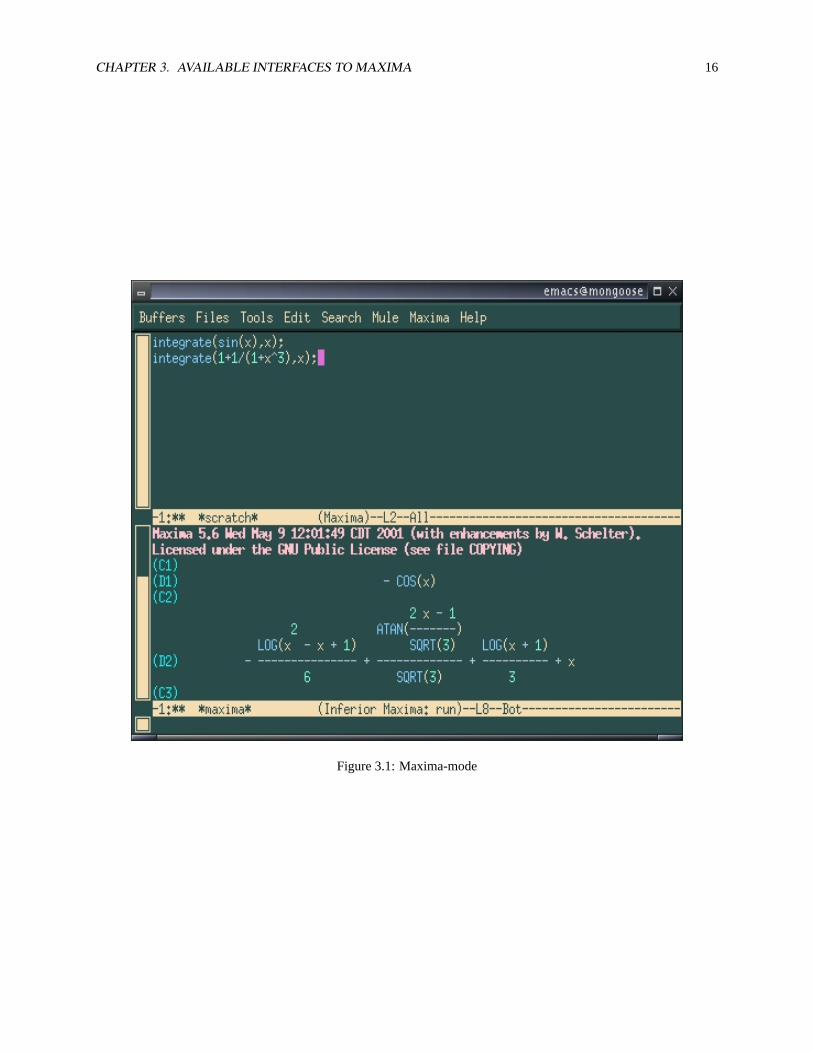
3.2.2. Maxima-mode
This mode is fairly basic, and is not dependant on LaTeX. It basically amounts to a text editor which allows you tosend lines to Maxima.
For moving around in the code, Maxima mode provides the followingMaxima mode has the following completions commands:
MotionKey DescriptionM-C-a Go to the beginning of the form.M-C-e Go to the end of the form.M-C-b Go to the beginning of the sexp.M-C-f Go to the end of the sexp.
ProcessKey DescriptionC-cC-p Start a Maxima process.C-cC-r Send the region to the Maxima process.C-cC-b Send the buffer to the Maxima process.C-cC-c Send the line to the Maxima process.C-cC-e Send the form to the Maxima process.C-cC-k Kill the Maxima process.C-cC-p Display the Maxima buffer.
Completion
Key DescriptionM-TAB Complete the Maxima symbol.
CommentsKey DescriptionC-c ; Comment the region.C-c : Uncomment the region.M-; Insert a short comment.C-c * Insert a comment environment.
IndentationKey DescriptionTAB Indent line.M-C-q Indent form.
Maxima help
Key DescriptionC-c C-d Get help on a (prompted for) subject.C-c C-m Read the manual.C-cC-h Get help with the symbol under point.C-cC-a Get apropos with the symbol under point.
MiscellaneousKey DescriptionM-h Mark the form.C-c) Check the region for balanced parentheses.C-c C-) Check the form for balanced parentheses.
When something is sent to Maxima, a buffer running an inferior Maxima process will appear. It can also be made toappear by using the commandC-c C-p. If an argument is given to a command to send information to Maxima, theregion (buffer, line, form) will first be checked to make sure the parentheses are balanced. The Maxima process canbe killed, after asking for confirmation withC-cC-k. To kill without confirmation, giveC-cC-k an argument.
The behaviour of indent can be changed by the commandM-x maxima-change-indent-style. The possibilitiesare:
Standard Standard indentation.
CHAPTER 3. AVAILABLE INTERFACES TO MAXIMA 16
Figure 3.1: Maxima-mode
CHAPTER 3. AVAILABLE INTERFACES TO MAXIMA 17
Perhaps smart Tries to guess an appropriate indentation, based on open parentheses, "do" loops, etc. A newline willre-indent the current line, then indent the new line an appropriate amount.
The default can be set by setting the value of the variablemaxima-newline-style to either’standard or’perhaps-smart.In all cases,M-x maxima-untab will remove a level of indentation.
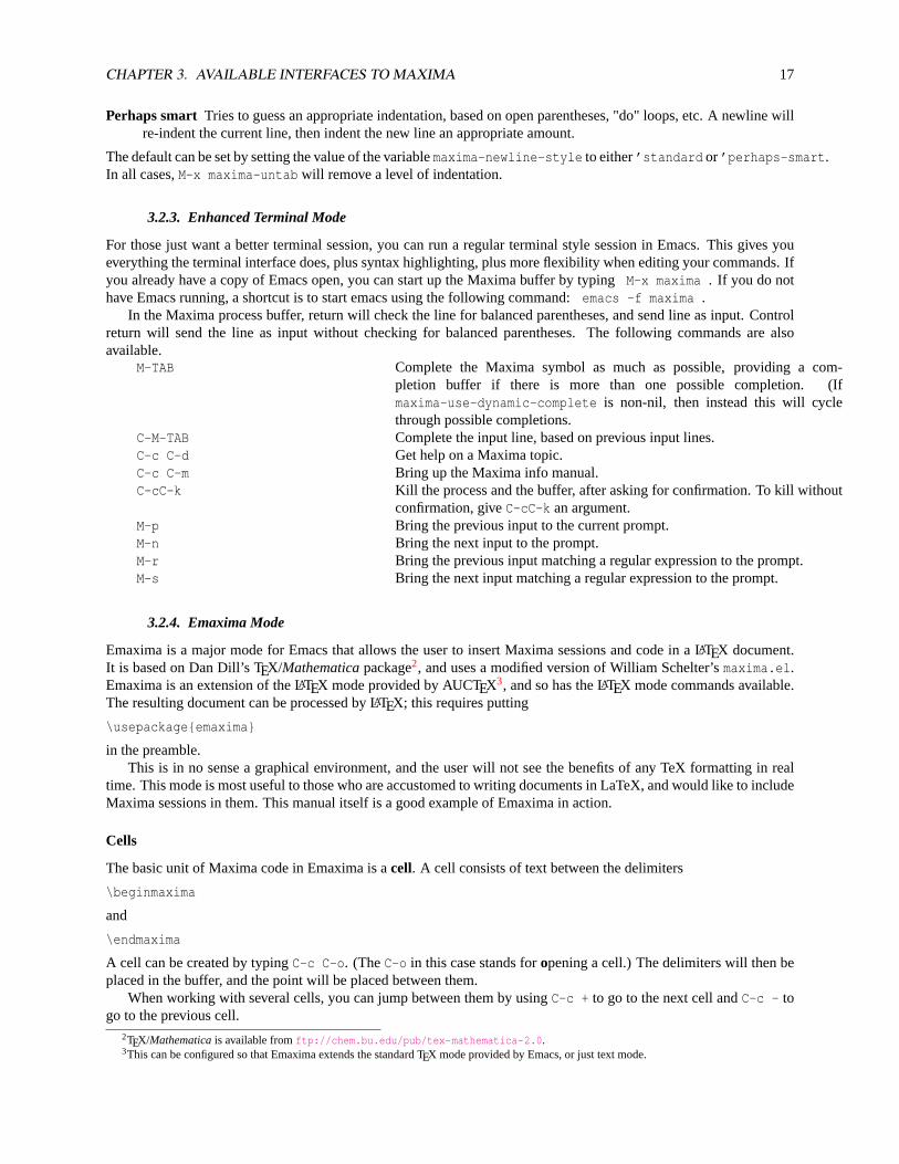
3.2.3. Enhanced Terminal Mode
For those just want a better terminal session, you can run a regular terminal style session in Emacs. This gives youeverything the terminal interface does, plus syntax highlighting, plus more flexibility when editing your commands. Ifyou already have a copy of Emacs open, you can start up the Maxima buffer by typingM-x maxima . If you do nothave Emacs running, a shortcut is to start emacs using the following command:emacs -f maxima .
In the Maxima process buffer, return will check the line for balanced parentheses, and send line as input. Controlreturn will send the line as input without checking for balanced parentheses. The following commands are alsoavailable.
M-TAB Complete the Maxima symbol as much as possible, providing a com-pletion buffer if there is more than one possible completion. (Ifmaxima-use-dynamic-complete is non-nil, then instead this will cyclethrough possible completions.
C-M-TAB Complete the input line, based on previous input lines.C-c C-d Get help on a Maxima topic.C-c C-m Bring up the Maxima info manual.C-cC-k Kill the process and the buffer, after asking for confirmation. To kill without
confirmation, giveC-cC-k an argument.M-p Bring the previous input to the current prompt.M-n Bring the next input to the prompt.M-r Bring the previous input matching a regular expression to the prompt.M-s Bring the next input matching a regular expression to the prompt.
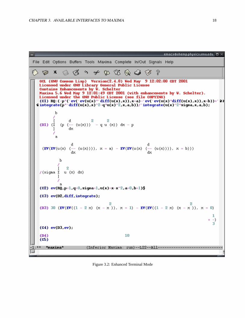
3.2.4. Emaxima Mode
Emaxima is a major mode for Emacs that allows the user to insert Maxima sessions and code in a LATEX document.It is based on Dan Dill’s TEX/Mathematicapackage2, and uses a modified version of William Schelter’smaxima.el.Emaxima is an extension of the LATEX mode provided by AUCTEX3, and so has the LATEX mode commands available.The resulting document can be processed by LATEX; this requires putting
\usepackage{emaxima}
in the preamble.This is in no sense a graphical environment, and the user will not see the benefits of any TeX formatting in real
time. This mode is most useful to those who are accustomed to writing documents in LaTeX, and would like to includeMaxima sessions in them. This manual itself is a good example of Emaxima in action.
Cells
The basic unit of Maxima code in Emaxima is acell. A cell consists of text between the delimiters
\beginmaxima
and
\endmaxima
A cell can be created by typingC-c C-o. (TheC-o in this case stands foropening a cell.) The delimiters will then beplaced in the buffer, and the point will be placed between them.
When working with several cells, you can jump between them by usingC-c + to go to the next cell andC-c - togo to the previous cell.
2TEX/Mathematicais available fromftp://chem.bu.edu/pub/tex-mathematica-2.0.3This can be configured so that Emaxima extends the standard TEX mode provided by Emacs, or just text mode.
CHAPTER 3. AVAILABLE INTERFACES TO MAXIMA 18
Figure 3.2: Enhanced Terminal Mode
CHAPTER 3. AVAILABLE INTERFACES TO MAXIMA 19
Figure 3.3: An Emaxima Session
CHAPTER 3. AVAILABLE INTERFACES TO MAXIMA 20
Evaluating cells
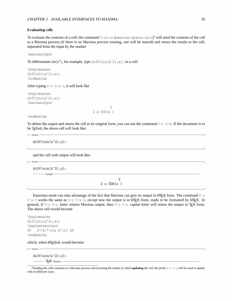
To evaluate the contents of a cell, the commandC-cC-uc (emaxima-update-cell)4 will send the contents of the cellto a Maxima process (if there is no Maxima process running, one will be started) and return the results to the cell,separated from the input by the marker
\maximaoutput
To differentiatesin(x2), for example, typediff(sin(xˆ2),x); in a cell:
\beginmaximadiff(sin(x^2),x);\endmaxima
After typingC-c C-u c, it will look like
\beginmaximadiff(sin(x^2),x);\maximaoutput
22 x COS(x )
\endmaxima
To delete the output and return the cell to its original form, you can use the commandC-c C-d. If the document is tobe TEXed, the above cell will look like:
Maxima
diff(sin(x^2),x);
and the cell with output will look like:
Maxima
diff(sin(x^2),x);
Output
22 x COS(x )
Emaxima mode can take advantage of the fact that Maxima can give its output in LATEX form. The commandC-cC-u C works the same asC-c C-u c, except now the output is in LATEX form, ready to be formatted by LATEX. Ingeneral, ifC-c C-u letter returns Maxima output, thenC-c C-u capital letter will return the output in TEX form.The above cell would become
\beginmaximadiff(sin(x^2),x);\maximatexoutput$$ 2\*x\*\cos x^{2} $$\endmaxima
which, when LATEXed, would become
Maxima
diff(sin(x^2),x);
TEX Output
4Sending the cells contents to a Maxima process and returning the results is calledupdating the cell, the prefixC-c C-u will be used to updatecells in different ways.
CHAPTER 3. AVAILABLE INTERFACES TO MAXIMA 21
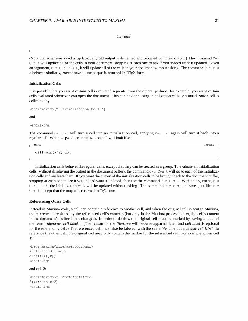
2x cosx2
(Note that whenever a cell is updated, any old output is discarded and replaced with new output.) The commandC-cC-u a will update all of the cells in your document, stopping at each one to ask if you indeed want it updated. Givenan argument,C-u C-c C-u a, it will update all of the cells in your document without asking. The commandC-c C-uA behaves similarly, except now all the output is returned in LATEX form.
Initialization Cells
It is possible that you want certain cells evaluated separate from the others; perhaps, for example, you want certaincells evaluated whenever you open the document. This can be done using initialization cells. An initialization cell isdelimited by
\beginmaxima[* Initialization Cell *]
and
\endmaxima
The commandC-c C-t will turn a cell into an initialization cell, applyingC-c C-t again will turn it back into aregular cell. When LATEXed, an initialization cell will look like
Maxima Initial
diff(sin(x^2),x);
Initialization cells behave like regular cells, except that they can be treated as a group. To evaluate all initializationcells (without displaying the output in the document buffer), the commandC-c C-u t will go to each of the initializa-tion cells and evaluate them. If you want the output of the initialization cells to be brought back to the document buffer,stopping at each one to see it you indeed want it updated, then use the commandC-c C-u i. With an argument,C-uC-c C-u i, the initialization cells will be updated without asking. The commandC-c C-u I behaves just likeC-cC-u i, except that the output is returned in TEX form.
Referencing Other Cells
Instead of Maxima code, a cell can contain a reference to another cell, and when the original cell is sent to Maxima,the reference is replaced by the referenced cell’s contents (but only in the Maxima process buffer, the cell’s contentin the document’s buffer is not changed). In order to do this, the original cell must be marked by having a label ofthe form<filename:cell label>. (The reason for thefilename will become apparent later, andcell label is optionalfor the referencing cell.) The referenced cell must also be labeled, with the samefilename but a uniquecell label. Toreference the other cell, the original cell need only contain the marker for the referenced cell. For example, given cell1:
\beginmaxima<filename:optional><filename:definef>diff(f(x),x);\endmaxima
and cell 2:
\beginmaxima<filename:definef>f(x):=sin(x^2);\endmaxima
CHAPTER 3. AVAILABLE INTERFACES TO MAXIMA 22
then the result of updating cell 1 (C-c C-u c) will be:
\beginmaxima<filename:optional><filename:definef>diff(f(x),x);\maximaoutput
2f(x) := SIN(x )
22 x COS(x )
\endmaxima
When LATEXed, the top line will contain a copy of the marker.
Maxima <filename:optional>
<filename:definef>diff(f(x),x);
Output
2f(x) := SIN(x )
22 x COS(x )
A cell can contain more than one reference, and referenced cells can themselves contain references.To aid in labelling the cells, the commandC-c C-x will prompt for a label name and label the cell. To aid in calling
references, the commandC-c C-TAB can be used for completing the thefilename andcell label parts of a reference,based on the current labels. Another option is to set the Emacs variableemaxima-abbreviations-allowed to t, say,by putting the line
(setq emaxima-abbreviations-allowed t)
in your .emacs file. This will allow thefilename andcell label parts of a reference to be abbreviated by enough of aprefix to uniquely identify it, followed by ellipses... For example, if there are cells labelled
<filename:long description><filename:lengthy description>
Then the reference
<...:le...>
will suffice to refer to the second label above.If you want the references in a cell to be replaced by the actual code, the commandC-c @ will expand all the
references and put the code into a separate buffer (so it will not affect the original document).
WEB
The reason for the ability to reference other cells is so that you can write what Donald Knuth calls literate programs.The idea is that the program is written in a form natural to the author rather than natural to the computer. (Anotheraspect of Knuth’s system is that the code is carefully documented, hence the name “literate programming”, but that isdone naturally in Emaxima.) Knuth called his original literate programming toolWEB, since, as he puts it, “the structureof a software program may be thought of as a web that is made up of many interconnected pieces.” Emaxima’s abilityin this respect is taken directly from TEX/Mathematica, and is ultimately based onWEB. To create a program, the “basecell” or “package cell” should contain a label of the form<filename:> (no cell label), and can contain references ofthe form<filename:part> (same file name as the base cell).
As a simple (and rather silly) example, suppose we want to create a program to sum the firstn squares. We couldstart:
CHAPTER 3. AVAILABLE INTERFACES TO MAXIMA 23
\beginmaxima<squaresum.max:>squaresum(n) := (
<squaresum.max:makelist><squaresum.max:squarelist><squaresum.max:addlist>);
\endmaxima
We would then need cells
\beginmaxima<squaresum.max:makelist>,L:makelist(k,k,1,n),\endmaxima
\beginmaxima<squaresum.max:squarelist><squaresum.max:definesquare>L:map(square,L),\endmaxima
\beginmaxima<squaresum.max:addlist>lsum(k,k,L)\endmaxima
and then we would also need:
\beginmaxima<squaresum.max:definesquare>square(k) := k^2,\endmaxima
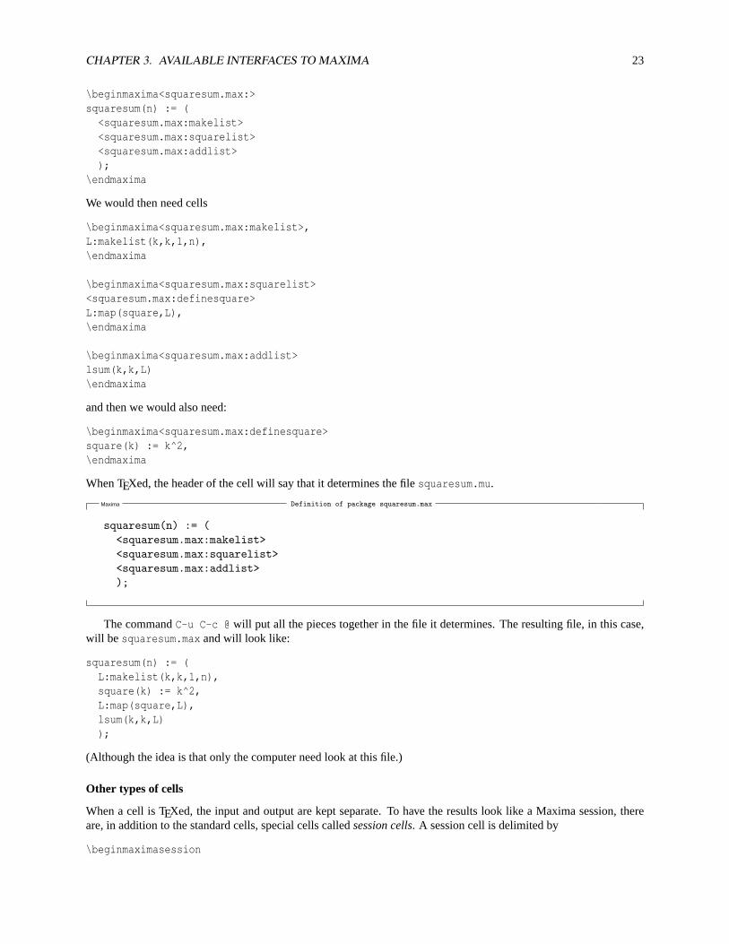
When TEXed, the header of the cell will say that it determines the filesquaresum.mu.
Maxima Definition of package squaresum.max
squaresum(n) := (<squaresum.max:makelist><squaresum.max:squarelist><squaresum.max:addlist>);
The commandC-u C-c @ will put all the pieces together in the file it determines. The resulting file, in this case,will be squaresum.max and will look like:
squaresum(n) := (L:makelist(k,k,1,n),square(k) := k^2,L:map(square,L),lsum(k,k,L));
(Although the idea is that only the computer need look at this file.)
Other types of cells
When a cell is TEXed, the input and output are kept separate. To have the results look like a Maxima session, thereare, in addition to the standard cells, special cells calledsession cells. A session cell is delimited by
\beginmaximasession
CHAPTER 3. AVAILABLE INTERFACES TO MAXIMA 24
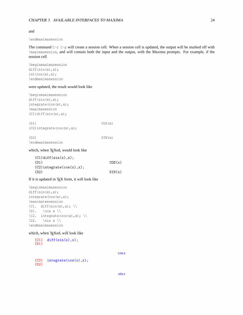
and
\endmaximasession
The commandC-c C-p will create a session cell. When a session cell is updated, the output will be marked off with\maximasession, and will contain both the input and the output, with the Maxima prompts. For example, if thesession cell
\beginmaximasessiondiff(sin(x),x);int(cos(x),x);\endmaximasession
were updated, the result would look like
\beginmaximasessiondiff(sin(x),x);integrate(cos(x),x);\maximasession(C1)diff(sin(x),x);
(D1) COS(x)(C2)integrate(cos(x),x);
(D2) SIN(x)\endmaximasession
which, when TEXed, would look like
(C1)diff(sin(x),x);(D1) COS(x)(C2)integrate(cos(x),x);(D2) SIN(x)
If it is updated in TEX form, it will look like
\beginmaximasessiondiff(sin(x),x);integrate(cos(x),x);\maximatexsession\C1. diff(sin(x),x); \\\D1. \cos x \\\C2. integrate(cos(x),x); \\\D2. \sin x \\\endmaximasession
which, when TEXed, will look like
(C1) diff(sin(x),x);(D1)
cosx
(C2) integrate(cos(x),x);(D2)
sinx

CHAPTER 3. AVAILABLE INTERFACES TO MAXIMA 25
For particularly long output lines inside the\maximatexsession part of a session cell, the command\DD willtypeset anything between the command and\\. Unfortunately, to take advantage of this, the output has to be brokenup by hand. If a session cell has not been updated, or has no output for some other reason, it will not appear when thedocument is TEXed.
There is one other type of cell, anoshow cell, which can be used to send Maxima a command, but won’t appear inthe TEXed output. A noshow cell can be created withC-c C-n, and will be delimited by
\beginmaximanoshow
and
\endmaximanoshow
Session cells and noshow cells cannot be initialization cells or part of packages.5
If the command to create one type of cell is called while inside another type of cell, the type of cell will be changed.So, for example, the commandC-c C-p from inside the cell
\beginmaximadiff(x*sin(x),x);\endmaxima
will result in
\beginmaximasessiondiff(x*sin(x),x);\endmaximasession
If a standard cell is an initialization cell or a package part, its type cannot be changed.
Miscellaneous
Some Maxima commands can be used even outside of cells. The commandC-c C-u l send the current line to aMaxima process, comment out the current line, and insert the Maxima output in the current buffer. The commandC-cC-u L will do the same, but return the result in LATEX form.
The commandC-c C-h will provide information on a prompted for function (like Maxima’sdescribe), andC-cC-i will give the Maxima info manual.
Finally, the Maxima process can be killed withC-c C-k.
Customizing EMaxima
There are a few things that you can do to customize Emaxima.By default, Emaxima is an extension of AUCTEX mode. This can be changed by changing the variableemaxima-use-tex.
The possible values are’auctex, ’tex andnil. Settingemaxima-use-tex (the default) to’auctex will make Emax-ima an extension of AUCTEX, setting it to’tex will make Emaxima an extension of Emacs’s default TEX mode, andsettingemaxima-use-tex to nil will make Emaxima an extension of text-mode. So, for example, putting
(setq emaxima-use-tex nil)
in your.emacs file will make Emaxima default to an extension of text mode.Whether or not the dots (. . . ) abbreviation is allowed in cell references is controlled by the elisp variableemaxima-abbreviations-allowed,
which is set tot by default. Setting this tonil will disallow the abbreviations, but will speed up package assembly.The LATEXed output can also be configured in a couple of ways. The lines that appear around cells when the
document is TEXed can be turned off with the command (in the LATEX document)
\maximalinesfalse
They can be turned back on with the command
5That could be changed, but I don’t know why it’d be useful.
CHAPTER 3. AVAILABLE INTERFACES TO MAXIMA 26
\maximalinestrue
The fonts used to display the Maxima input and output in a cell are by defaultcmtt10. They can be changed,seperately, by changing the TEX values of\maximainputfont and\maximaoutputfont. So, for example, to usecmtt12 as the input font, use the command
\font\maximainputfont = cmtt12
The spacing in the cells can be controlled by changing the TEX variables\maximainputbaselineskip and\maximaoutputbaselineskip,and so to increase the space between the lines of the output, the command
\maximaoutputbaselineskip = 14pt
could be used. The amount of space that appears before a cell can be changed by changing the value of\premaximaspace(by default, 0pt), and that after a cell can be changed by changing the value of\postmaximaspace (by default, 1.5ex).
Session cells can be configured similarly. Lines can be placed around a Maxima session with the command
\maximasessionlinestrue
and they can be turned back off with
\maximasessionlinesfalse
The font can be changed by changing the value of\maximasessionfont. The color of the prompts when the sessionis in TEX form is controlled by\maximapromptcolor, by default red, the colors of the input lines and output lines are controlled by\maximainputcolorand\maximaoutputcolor, respectively. So the command
\def\maximainputcolor{green}
would make the input in a TEXed session green. The session can be TEXed without the colors by using the command\maximasessionnocolor. The baselineskip is set by\maximasessionbaselineskip for normal session cells, andby \maixmatexsessionbaselineskip for TEX sessions. The amount of space that appears before a session cell canbe changed by changing the value of\premaximasessionspace (by default, 0pt), and that after a cell can be changedby changing the value of\postmaximasessionspace (by default, 1.5 ex).
Emaxima mode commands
Key DescriptionC-c C-o Create a (standard) cell.C-c C-p Create a session cell.C-c C-n Create a noshow cell.C-c + Go the the next cell.C-c - Go to the previous cell.C-c C-u a Update all of the cells. With an argument, don’t ask before updating.C-c C-u A Update all of the cells in TEX form. With an argument don’t ask before
updating.C-c C-u t Evaluate all of the initialization cells.C-c C-u i Update all of the initialization cells. With an argument, don’t ask before
updating.C-c C-u I Update all of the initialization cells in TEX form. With an argument, don’t
ask before updating.C-c C-u s Update all of the session cells in TEX form. With an argument, don’t ask
before updating.C-c C-k Kill the current Maxima core - this will lose all data entered into the maxima
system up until this point by other cells.
Commands only available in cells.
CHAPTER 3. AVAILABLE INTERFACES TO MAXIMA 27
Key DescriptionC-c C-v Send the current cell to the Maxima process.C-c C-u c Update the current cell.C-c C-u C Update the current cell in TEX form.C-c C-d Delete the output from the current cell.C-c C-t Toggle whether or not the current cell is an initialization cell.C-c C-x Insert a heading for the cell indicating that it’s part of a package.C-c @ Assemble the references contained in the cell. With an argument, assemble
the package that the cell defines.C-c C-TAB Complete a reference within a cell.
Commands only available outside of cells.
Key DescriptionC-c C-u l Send the current line to Maxima, and replace the line with the Maxima out-
put.C-c C-u L Send the current line to Maxima, and replace the line with the Maxima output
in TEX form.
AUCTEX commands
Inserting commands
Key DescriptionC-c C-e Insert an environment.C-c C-s Insert a section.C-c ] Close an environment.C-c C-j Insert an item into a list." Smart quote.$ Smart dollar sign.C-c @ Insert double brace.C-c C-m Insert TEX macro.M-TAB Complete TEX macro.
Formatting
Key DescriptionC-c C-q C-r Format region.C-c C-q C-s Format section.C-c C-q C-e Format environment.C-c . Mark an environment.C-c * Mark a section.
Commenting
Key DescriptionC-c ; Comment a region.C-u C-c ; Uncomment a region.C-c % Comment a paragraph.C-u C-c % Uncomment a paragraph.
Font selectionKey DescriptionC-c C-f C-b Bold.C-c C-f C-i Italics.C-c C-f C-r Roman.C-c C-f C-e Emphasized.C-c C-f C-t Typewriter.C-c C-f C-s Slanted.C-c C-f C-d Delete font.C-u C-c C-f Change font.
CHAPTER 3. AVAILABLE INTERFACES TO MAXIMA 28
Running TEX
(Commands:TeX, TeX Interactive, LaTeX, LaTeX Interactive, SliTeX, View, Print, BibTeX, Index, Check,File, Spell.)
Key DescriptionC-c C-c Run a command on the master file.C-c C-r Run a command on the current region.C-c C-b Run a command on the buffer.C-c ‘ Go to the next error.C-c C-k Kill the TEX process.C-c C-l Center the output buffer.C-c C-ˆ Switch to the master file.C-c C-w Toggle debug of overful boxes.
3.3 Xmaxima
CHAPTER 3. AVAILABLE INTERFACES TO MAXIMA 29
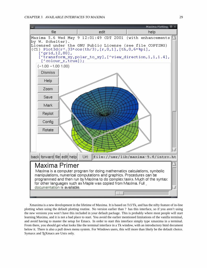
Xmaxima is a new development in the lifetime of Maxima. It is based on Tcl/Tk, and has the nifty feature of in-lineplotting when using the default plotting routine. No version earlier than ? has this interface, so if you aren’t usingthe new versions you won’t have this included in your default package. This is probably where most people will startlearning Maxima, and it is not a bad place to start. You avoid the earlier mentioned limitations of the vanilla terminal,and avoid having to master the setup for Emacs. In order to start this interface simply type xmaxima in a terminal.From there, you should get what looks like the terminal interface in a Tk window, with an introductory html documentbelow it. There is also a pull down menu system. For Windows users, this will more than likely be the default choice.Symaxx and TEXmacs are Unix only.

CHAPTER 3. AVAILABLE INTERFACES TO MAXIMA 30
3.4 Symaxx
In the words of its creator Markus Nentwig “Symaxx provides those 5% of features, that are needed to do 95% ofyour work.” Perhaps the best description of its display is that of a mathematical flowchart - it indicates relationshipsbetween cells with arrows, and allows free placement of expressions on a canvas. It is more graphical than any of theother Maxima interfaces, and although input is still ascii based the output is formatted. It is based on Perl and Tk,both of which are required to run it. This interface tends, at least in the experience of this author, to be a bit resourceintensive, but allows some page formatting possibilities which make it a very interesting program. We will show yousome of its features here, and if you decide to use this interfacethe Symaxx manual is a highly recommended read.
Symaxx uses a fairly basic display format - each unit of mathematical input and output is labeled with an IDnumber, which one can use to refer to that particular unit elsewhere in your document. There are three levels to eachunit - the input box, which displays the command input into Maxima, the output box, which displays the results, and
CHAPTER 3. AVAILABLE INTERFACES TO MAXIMA 31
the documentation box, where you can record information and descriptions which are not intended to be evaluated.This may take a little getting used to - pressing return once you are done creating the input expression doesn’t evaluateit, but only sends it to the formatter used by Symaxx to create a graphical representation of the input. To send thecommand to Maxima, you press the evaluate button.
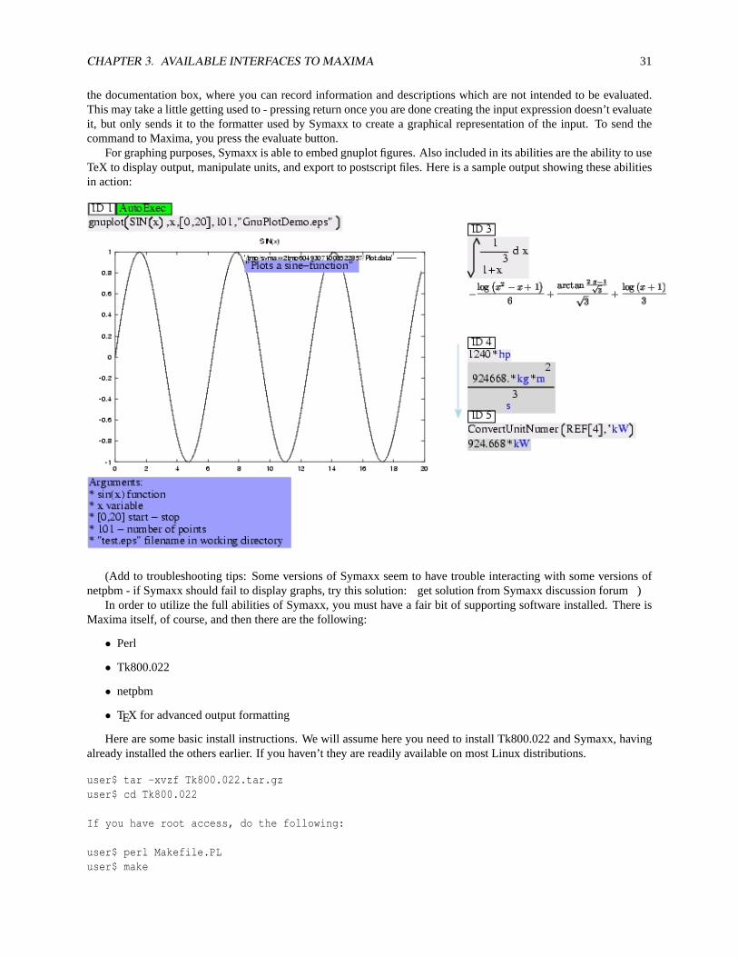
For graphing purposes, Symaxx is able to embed gnuplot figures. Also included in its abilities are the ability to useTeX to display output, manipulate units, and export to postscript files. Here is a sample output showing these abilitiesin action:
(Add to troubleshooting tips: Some versions of Symaxx seem to have trouble interacting with some versions ofnetpbm - if Symaxx should fail to display graphs, try this solution: get solution from Symaxx discussion forum )
In order to utilize the full abilities of Symaxx, you must have a fair bit of supporting software installed. There isMaxima itself, of course, and then there are the following:
• Perl
• Tk800.022
• netpbm
• TEX for advanced output formatting
Here are some basic install instructions. We will assume here you need to install Tk800.022 and Symaxx, havingalready installed the others earlier. If you haven’t they are readily available on most Linux distributions.
user$ tar -xvzf Tk800.022.tar.gzuser$ cd Tk800.022
If you have root access, do the following:
user$ perl Makefile.PLuser$ make
CHAPTER 3. AVAILABLE INTERFACES TO MAXIMA 32
user$ make test (optional)user$ suPassword:root$ make install
if you don’t have root access, use
user$ perl Makefile.PL LIB=/home/(place to install) oruser$ perl Makefile.PL PREFIX=/home/(place to install).user$ make; make install
Find the location of the folder ‘Tk’ in the folder you gave as argument to LIB or PREFIX. Now you’ll have tochange the first line in ‘symaxx’ and ‘Symaxx2/Watchdog’ to include the Tk library. Append a-I /home/(where you installed Tk)/(The folder that contains Tk) as in #!/usr/bin/perl -w -I /home/somewhere/
Then simply decompress Symaxx in the directory of your choice. If perl is not in /usr/bin, you’ll have to changethe first line of the files ‘symaxx’ and ‘Symaxx2/Watchdog’ to the location on your system, as found by ‘whereis perl’.
3.5 TEXmacs
TEXmacs is a new WYSIWYG scientific editor, and it has the ability to interface with many computer algebra systems,including Maxima. This program takes advantage of the TEX output Maxima can produce to format it’s output. Tolaunch Maxima inside of TEXmacs you go up to the menu and select Insert -> sessions -> maxima. Then things worklike they do in xmaxima or Emacs. This is probably the most visually appealing way to run Maxima. You can insert amaxima session in TeXmacs by selecting Insert->session->maxima from the menu. From there the interface will feelpretty much like a regular terminal.

CHAPTER 3. AVAILABLE INTERFACES TO MAXIMA 33
Figure 3.4: TeXmacs with a Maxima Session
CHAPTER 4
The Basics - What you need to know to operate in Maxima
Here we will attempt to address universal concepts which you will need to know when using Maxima for a widevariety of tasks.
4.1 The Very Beginning
All computer algebra systems have syntactical rules, i.e. a structured language by which the user communicates his/hercommands to the system. Without being able to communicate in this language, it is impossible to accomplish anythingin such as system. So we will attempt to describe herein the basics.
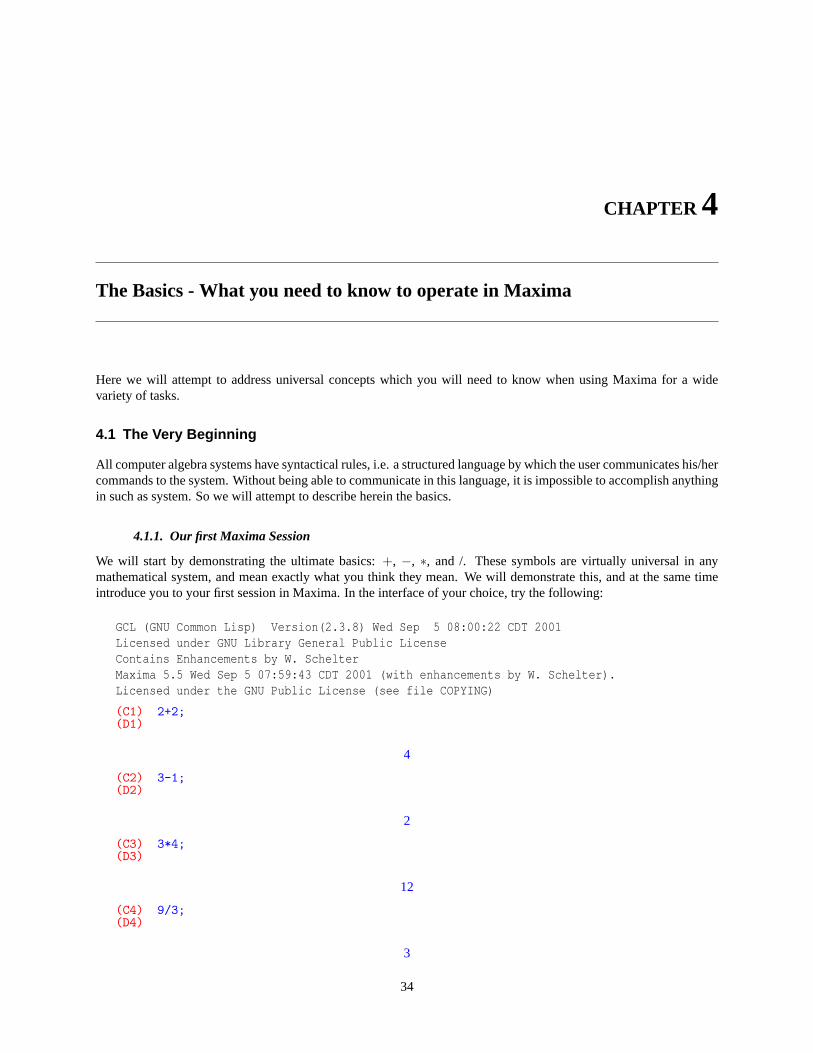
4.1.1. Our first Maxima Session
We will start by demonstrating the ultimate basics:+, −, ∗, and /. These symbols are virtually universal in anymathematical system, and mean exactly what you think they mean. We will demonstrate this, and at the same timeintroduce you to your first session in Maxima. In the interface of your choice, try the following:
GCL (GNU Common Lisp) Version(2.3.8) Wed Sep 5 08:00:22 CDT 2001Licensed under GNU Library General Public LicenseContains Enhancements by W. SchelterMaxima 5.5 Wed Sep 5 07:59:43 CDT 2001 (with enhancements by W. Schelter).Licensed under the GNU Public License (see file COPYING)
(C1) 2+2;(D1)
4
(C2) 3-1;(D2)
2
(C3) 3*4;(D3)
12
(C4) 9/3;(D4)
3
34
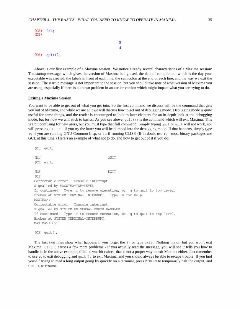
CHAPTER 4. THE BASICS - WHAT YOU NEED TO KNOW TO OPERATE IN MAXIMA 35
(C5) 9/4;(D5)
94
(C6) quit();
Above is our first example of a Maxima session. We notice already several characteristics of a Maxima session:The startup message, which gives the version of Maxima being used, the date of compilation, which is the day yourexecutable was created, the labels in front of each line, the semicolon at the end of each line, and the way we exit thesession. The startup message is not important to the session, but you should take note of what version of Maxima youare using, especially if there is a known problem in an earlier version which might impact what you are trying to do.
Exiting a Maxima Session
You want to be able to get out of what you get into. So the first command we discuss will be the command that getsyou out of Maxima, and while we are at it we will discuss how to get out of debugging mode. Debugging mode is quiteuseful for some things, and the reader is encouraged to look to later chapters for an in-depth look at the debuggingmode, but for now we will stick to basics. As you see above,quit(); is the command which will exit Maxima. Thisis a bit confusing for new users, but you must type that full command. Simply typingquit or exit will not work, norwill pressingCTRL-C - if you try the latter you will be dumped into the debugging mode. If that happens, simply type:q if you are running GNU Common Lisp, or:a if running CLISP. (If in doubt use:q - most binary packages useGCL at this time.) Here’s an example of what not to do, and how to get out of it if you do:
(C1) quit;
(D1) QUIT(C2) exit;
(D2) EXIT(C3)Correctable error: Console interrupt.Signalled by MACSYMA-TOP-LEVEL.If continued: Type :r to resume execution, or :q to quit to top level.Broken at SYSTEM:TERMINAL-INTERRUPT. Type :H for Help.MAXIMA> >Correctable error: Console interrupt.Signalled by SYSTEM:UNIVERSAL-ERROR-HANDLER.If continued: Type :r to resume execution, or :q to quit to top level.Broken at SYSTEM:TERMINAL-INTERRUPT.MAXIMA> > >:q
(C3) quit();
The first two lines show what happens if you forget the() or typeexit. Nothing major, but you won’t exitMaxima. CTRL-C causes a few more problems - if you actually read the message, you will see it tells you how tohandle it. In the above example,CTRL-C was hit twice - that is not a proper way to exit Maxima either. Just rememberto use:q to exit debugging andquit(); to exit Maxima, and you should always be able to escape trouble. If you findyouself trying to read a long output going by quickly on a terminal, pressCTRL-S to temporarily halt the output, andCTRL-Q to resume.
CHAPTER 4. THE BASICS - WHAT YOU NEED TO KNOW TO OPERATE IN MAXIMA 36
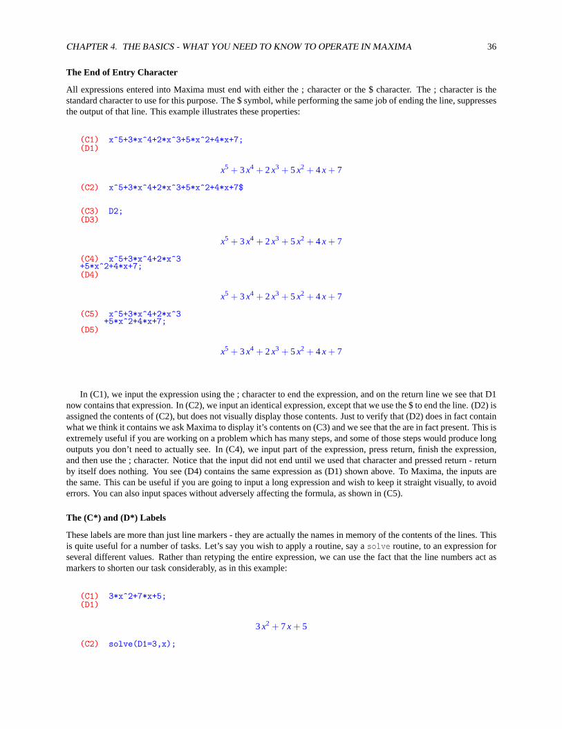
The End of Entry Character
All expressions entered into Maxima must end with either the ; character or the $ character. The ; character is thestandard character to use for this purpose. The $ symbol, while performing the same job of ending the line, suppressesthe output of that line. This example illustrates these properties:
(C1) x^5+3*x^4+2*x^3+5*x^2+4*x+7;(D1)
x5 + 3x4 + 2x3 + 5x2 + 4x + 7
(C2) x^5+3*x^4+2*x^3+5*x^2+4*x+7$
(C3) D2;(D3)
x5 + 3x4 + 2x3 + 5x2 + 4x + 7
(C4) x^5+3*x^4+2*x^3+5*x^2+4*x+7;(D4)
x5 + 3x4 + 2x3 + 5x2 + 4x + 7
(C5) x^5+3*x^4+2*x^3+5*x^2+4*x+7;
(D5)
x5 + 3x4 + 2x3 + 5x2 + 4x + 7
In (C1), we input the expression using the ; character to end the expression, and on the return line we see that D1now contains that expression. In (C2), we input an identical expression, except that we use the $ to end the line. (D2) isassigned the contents of (C2), but does not visually display those contents. Just to verify that (D2) does in fact containwhat we think it contains we ask Maxima to display it’s contents on (C3) and we see that the are in fact present. This isextremely useful if you are working on a problem which has many steps, and some of those steps would produce longoutputs you don’t need to actually see. In (C4), we input part of the expression, press return, finish the expression,and then use the ; character. Notice that the input did not end until we used that character and pressed return - returnby itself does nothing. You see (D4) contains the same expression as (D1) shown above. To Maxima, the inputs arethe same. This can be useful if you are going to input a long expression and wish to keep it straight visually, to avoiderrors. You can also input spaces without adversely affecting the formula, as shown in (C5).
The (C*) and (D*) Labels
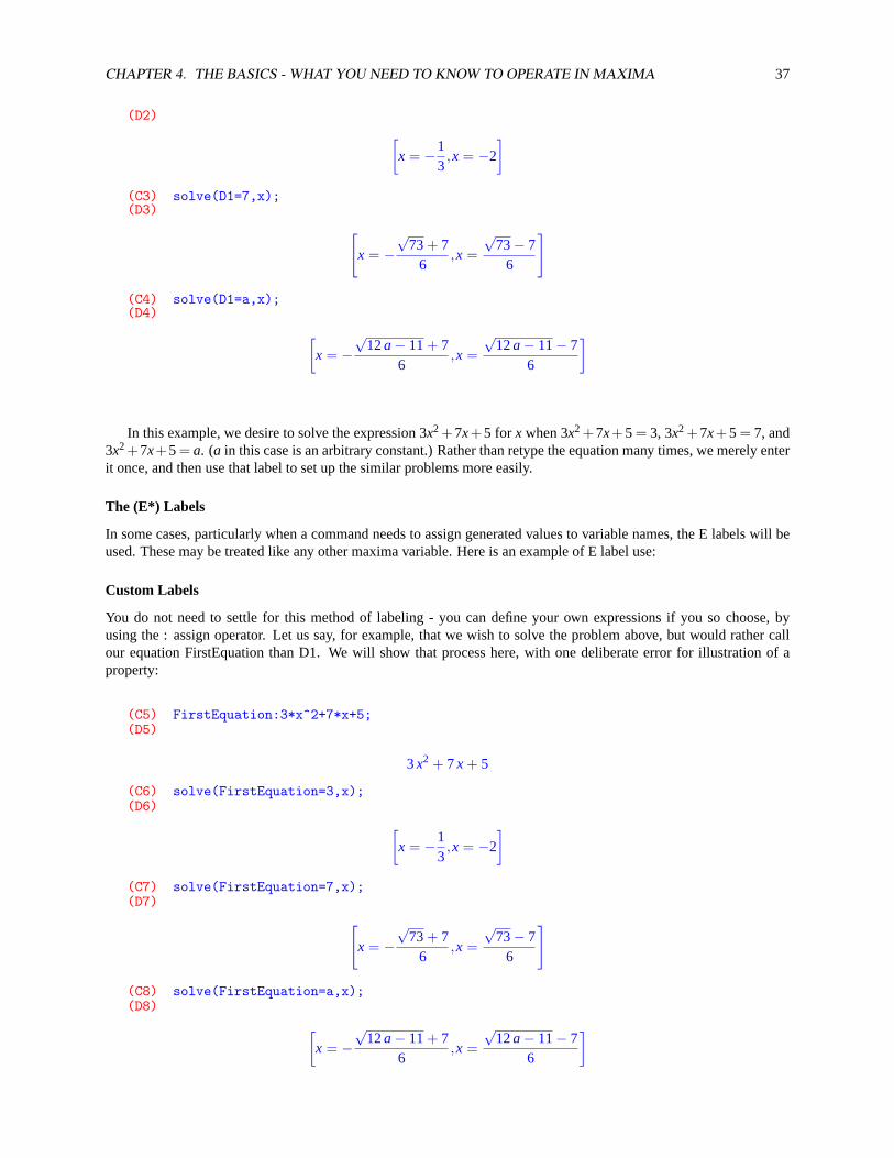
These labels are more than just line markers - they are actually the names in memory of the contents of the lines. Thisis quite useful for a number of tasks. Let’s say you wish to apply a routine, say asolve routine, to an expression forseveral different values. Rather than retyping the entire expression, we can use the fact that the line numbers act asmarkers to shorten our task considerably, as in this example:
(C1) 3*x^2+7*x+5;(D1)
3x2 + 7x + 5
(C2) solve(D1=3,x);
CHAPTER 4. THE BASICS - WHAT YOU NEED TO KNOW TO OPERATE IN MAXIMA 37
(D2) [x = −1
3,x = −2
](C3) solve(D1=7,x);(D3) [
x = −√
73+ 76
,x =√
73− 76
]
(C4) solve(D1=a,x);(D4) [
x = −√
12a− 11+ 76
,x =√
12a− 11− 76
]
In this example, we desire to solve the expression 3x2 +7x+5 for x when 3x2 +7x+5 = 3, 3x2 +7x+5 = 7, and3x2+7x+5= a. (a in this case is an arbitrary constant.) Rather than retype the equation many times, we merely enterit once, and then use that label to set up the similar problems more easily.
The (E*) Labels
In some cases, particularly when a command needs to assign generated values to variable names, the E labels will beused. These may be treated like any other maxima variable. Here is an example of E label use:
Custom Labels
You do not need to settle for this method of labeling - you can define your own expressions if you so choose, byusing the : assign operator. Let us say, for example, that we wish to solve the problem above, but would rather callour equation FirstEquation than D1. We will show that process here, with one deliberate error for illustration of aproperty:
(C5) FirstEquation:3*x^2+7*x+5;(D5)
3x2 + 7x + 5
(C6) solve(FirstEquation=3,x);(D6) [
x = −13,x = −2
](C7) solve(FirstEquation=7,x);(D7) [
x = −√
73+ 76
,x =√
73− 76
]
(C8) solve(FirstEquation=a,x);(D8) [
x = −√
12a− 11+ 76
,x =√
12a− 11− 76
]
CHAPTER 4. THE BASICS - WHAT YOU NEED TO KNOW TO OPERATE IN MAXIMA 38
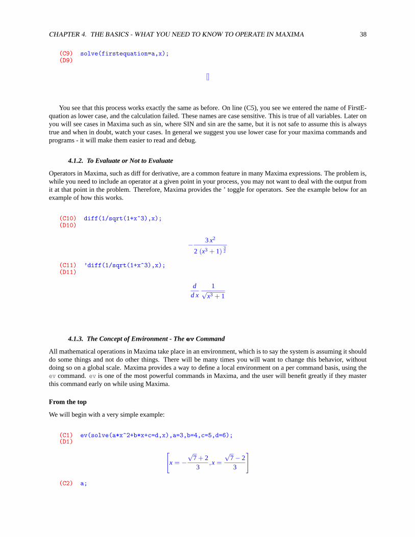
(C9) solve(firstequation=a,x);(D9)
[]
You see that this process works exactly the same as before. On line (C5), you see we entered the name of FirstE-quation as lower case, and the calculation failed. These names are case sensitive. This is true of all variables. Later onyou will see cases in Maxima such as sin, where SIN and sin are the same, but it is not safe to assume this is alwaystrue and when in doubt, watch your cases. In general we suggest you use lower case for your maxima commands andprograms - it will make them easier to read and debug.
4.1.2. To Evaluate or Not to Evaluate
Operators in Maxima, such as diff for derivative, are a common feature in many Maxima expressions. The problem is,while you need to include an operator at a given point in your process, you may not want to deal with the output fromit at that point in the problem. Therefore, Maxima provides the ’ toggle for operators. See the example below for anexample of how this works.
(C10) diff(1/sqrt(1+x^3),x);(D10)
− 3x2
2 (x3 + 1)32
(C11) ’diff(1/sqrt(1+x^3),x);(D11)
dd x
1√x3 + 1
4.1.3. The Concept of Environment - Theev Command
All mathematical operations in Maxima take place in an environment, which is to say the system is assuming it shoulddo some things and not do other things. There will be many times you will want to change this behavior, withoutdoing so on a global scale. Maxima provides a way to define a local environment on a per command basis, using theev command.ev is one of the most powerful commands in Maxima, and the user will benefit greatly if they masterthis command early on while using Maxima.
From the top
We will begin with a very simple example:
(C1) ev(solve(a*x^2+b*x+c=d,x),a=3,b=4,c=5,d=6);(D1) [
x = −√
7 + 23
,x =√
7− 23
]
(C2) a;
CHAPTER 4. THE BASICS - WHAT YOU NEED TO KNOW TO OPERATE IN MAXIMA 39
(D2)
a
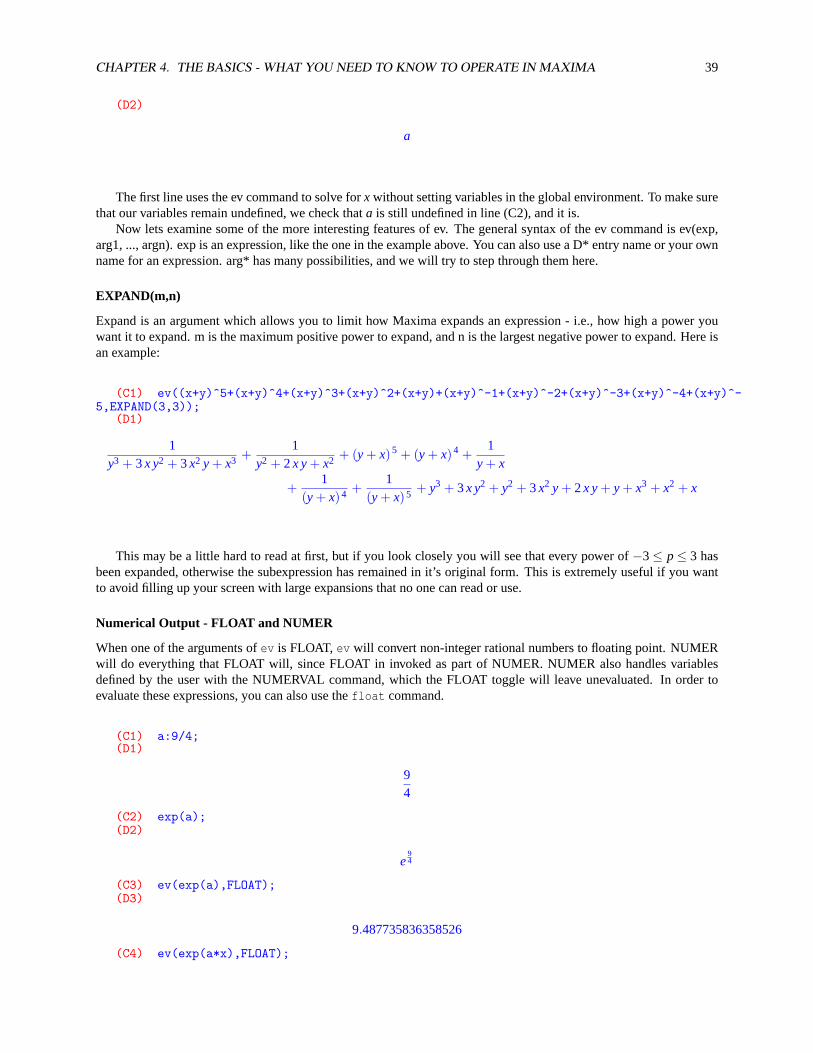
The first line uses the ev command to solve forx without setting variables in the global environment. To make surethat our variables remain undefined, we check thata is still undefined in line (C2), and it is.
Now lets examine some of the more interesting features of ev. The general syntax of the ev command is ev(exp,arg1, ..., argn). exp is an expression, like the one in the example above. You can also use a D* entry name or your ownname for an expression. arg* has many possibilities, and we will try to step through them here.
EXPAND(m,n)
Expand is an argument which allows you to limit how Maxima expands an expression - i.e., how high a power youwant it to expand. m is the maximum positive power to expand, and n is the largest negative power to expand. Here isan example:
(C1) ev((x+y)^5+(x+y)^4+(x+y)^3+(x+y)^2+(x+y)+(x+y)^-1+(x+y)^-2+(x+y)^-3+(x+y)^-4+(x+y)^-5,EXPAND(3,3));
(D1)
1y3 + 3x y2 + 3x2 y + x3 +
1y2 + 2x y+ x2 + (y + x)5 + (y + x)4 +
1y + x
+1
(y + x)4 +1
(y + x)5 + y3 + 3x y2 + y2 + 3x2 y + 2x y+ y + x3 + x2 + x
This may be a little hard to read at first, but if you look closely you will see that every power of−3≤ p≤ 3 hasbeen expanded, otherwise the subexpression has remained in it’s original form. This is extremely useful if you wantto avoid filling up your screen with large expansions that no one can read or use.
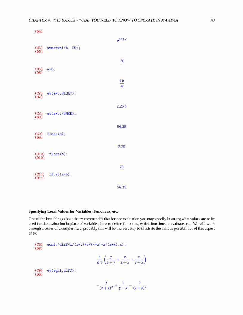
Numerical Output - FLOAT and NUMER
When one of the arguments ofev is FLOAT, ev will convert non-integer rational numbers to floating point. NUMERwill do everything that FLOAT will, since FLOAT in invoked as part of NUMER. NUMER also handles variablesdefined by the user with the NUMERVAL command, which the FLOAT toggle will leave unevaluated. In order toevaluate these expressions, you can also use thefloat command.
(C1) a:9/4;(D1)
94
(C2) exp(a);(D2)
e94
(C3) ev(exp(a),FLOAT);(D3)
9.487735836358526
(C4) ev(exp(a*x),FLOAT);
CHAPTER 4. THE BASICS - WHAT YOU NEED TO KNOW TO OPERATE IN MAXIMA 40
(D4)
e2.25x
(C5) numerval(b, 25);(D5)
[b]
(C6) a*b;(D6)
9b4
(C7) ev(a*b,FLOAT);(D7)
2.25b
(C8) ev(a*b,NUMER);(D8)
56.25
(C9) float(a);(D9)
2.25
(C10) float(b);(D10)
25
(C11) float(a*b);(D11)
56.25
Specifying Local Values for Variables, Functions, etc.
One of the best things about the ev command is that for one evaluation you may specify in an arg what values are to beused for the evaluation in place of variables, how to define functions, which functions to evaluate, etc. We will workthrough a series of examples here, probably this will be the best way to illustrate the various possibilities of this aspectof ev.
(C8) eqn1:’diff(x/(x+y)+y/(y+z)+z/(z+x),x);(D8)
dd x
(y
z+ y+
zz+ x
+x
y + x
)(C9) ev(eqn1,diff);(D9)
− z(z+ x)2 +
1y + x
− x(y + x)2

CHAPTER 4. THE BASICS - WHAT YOU NEED TO KNOW TO OPERATE IN MAXIMA 41
(C10) ev(eqn1,y=x+z);(D10)
dd x
(z+ x
2z+ x+
xz+ 2x
+z
z+ x
)(C11) ev(eqn1,y=x+z,diff);(D11)
12z+ x
− z+ x(2z+ x)2 +
1z+ 2x
− 2x(z+ 2x)2 −
z(z+ x)2
In this example, we define eqn1 to be the derivative of a function, but use the ’ character in front of the diff operatorto notify Maxima that we don’t want it to evaluate that derivative at this time. (More on that in the ?? section.) In thenext line, we use the ev with the diff argument, which instructs ev to take all derivatives in this expression. Now, let’ssay we want to definey as a function ofz andx, but again avoid evaluating the derivative. We supply our definitionof y as an argument to ev, and in (D3) we see that the substitution has been made. Now, let’s evaluate the derivativeafter the substitution has been made. We work as before, except this time we supply both the new definition ofy andthe diff argument, telling ev to make the substitution and then take the derivative. In this particular case, the order ofthe arguments does not matter. The case where it will matter is if you are making multiple substitutions - then they arehandled in sequence from left to right.
(need example here, one where the difference is noticeable).
We can also locally define functions:
(C12) eqn4:f(x,y)*’diff(g(x,y),x);(D12)
f (x,y)(
dd x
g(x,y))
(C13) ev(eqn4,f(x,y)=x+y,g(x,y)=x^2+y^2);(D13)
(y + x)(
dd x
(y2 + x2))
(C14) ev(eqn4,f(x,y)=x+y,g(x,y)=x^2+y^2,DIFF);(D14)
2x (y + x)
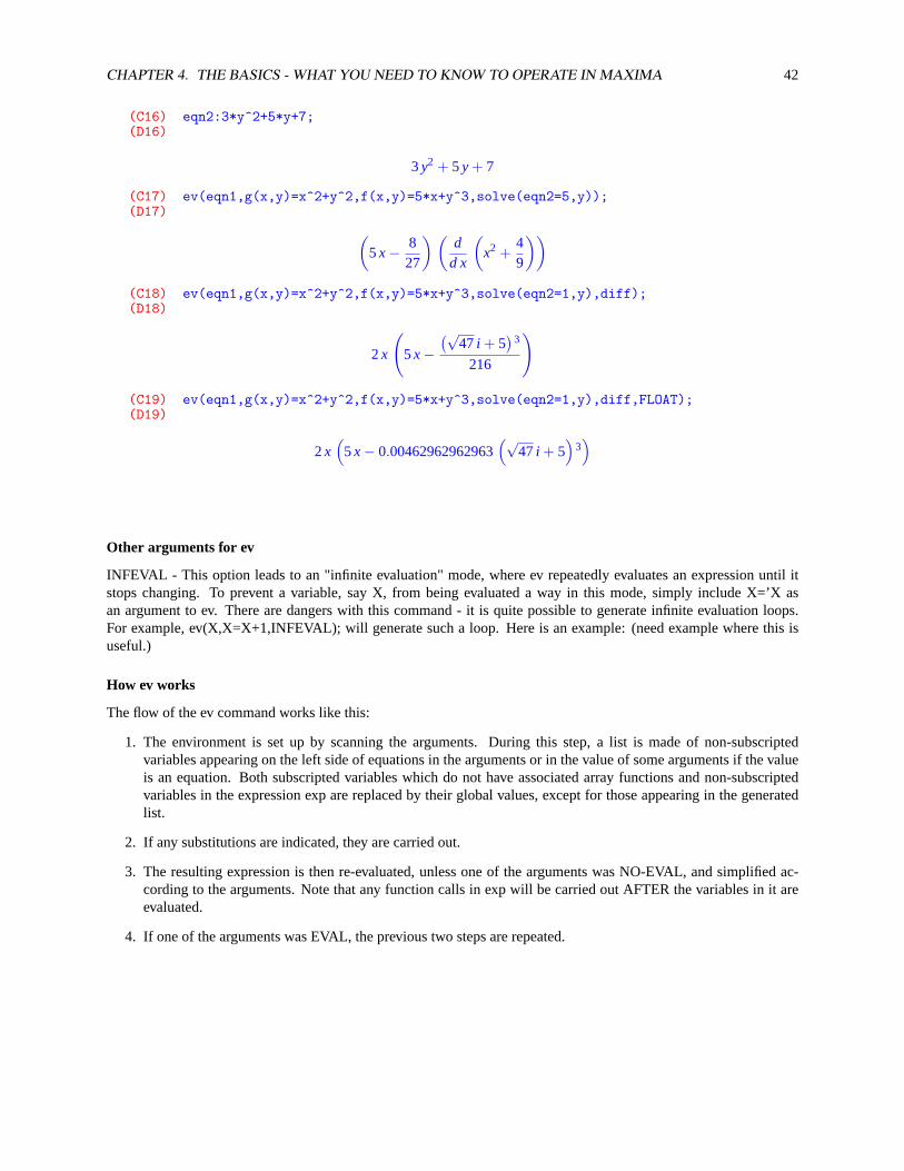
(At the moment, ev seems to take only the first argument in the following example from solve: the manual seemsto indicate it should be taking both as a list??)
(C15) eqn1:f(x,y)*’diff(g(x,y),x);(D15)
f (x,y)(
dd x
g(x,y))
CHAPTER 4. THE BASICS - WHAT YOU NEED TO KNOW TO OPERATE IN MAXIMA 42
(C16) eqn2:3*y^2+5*y+7;(D16)
3y2 + 5y + 7
(C17) ev(eqn1,g(x,y)=x^2+y^2,f(x,y)=5*x+y^3,solve(eqn2=5,y));(D17) (
5x− 827
) (d
d x
(x2 +
49
))(C18) ev(eqn1,g(x,y)=x^2+y^2,f(x,y)=5*x+y^3,solve(eqn2=1,y),diff);(D18)
2x
(5x−
(√47i + 5
)3
216
)
(C19) ev(eqn1,g(x,y)=x^2+y^2,f(x,y)=5*x+y^3,solve(eqn2=1,y),diff,FLOAT);(D19)
2x(
5x− 0.00462962962963(√
47i + 5)
3)
Other arguments for ev
INFEVAL - This option leads to an "infinite evaluation" mode, where ev repeatedly evaluates an expression until itstops changing. To prevent a variable, say X, from being evaluated a way in this mode, simply include X=’X asan argument to ev. There are dangers with this command - it is quite possible to generate infinite evaluation loops.For example, ev(X,X=X+1,INFEVAL); will generate such a loop. Here is an example: (need example where this isuseful.)
How ev works
The flow of the ev command works like this:
1. The environment is set up by scanning the arguments. During this step, a list is made of non-subscriptedvariables appearing on the left side of equations in the arguments or in the value of some arguments if the valueis an equation. Both subscripted variables which do not have associated array functions and non-subscriptedvariables in the expression exp are replaced by their global values, except for those appearing in the generatedlist.
2. If any substitutions are indicated, they are carried out.
3. The resulting expression is then re-evaluated, unless one of the arguments was NO-EVAL, and simplified ac-cording to the arguments. Note that any function calls in exp will be carried out AFTER the variables in it areevaluated.
4. If one of the arguments was EVAL, the previous two steps are repeated.
CHAPTER 4. THE BASICS - WHAT YOU NEED TO KNOW TO OPERATE IN MAXIMA 43
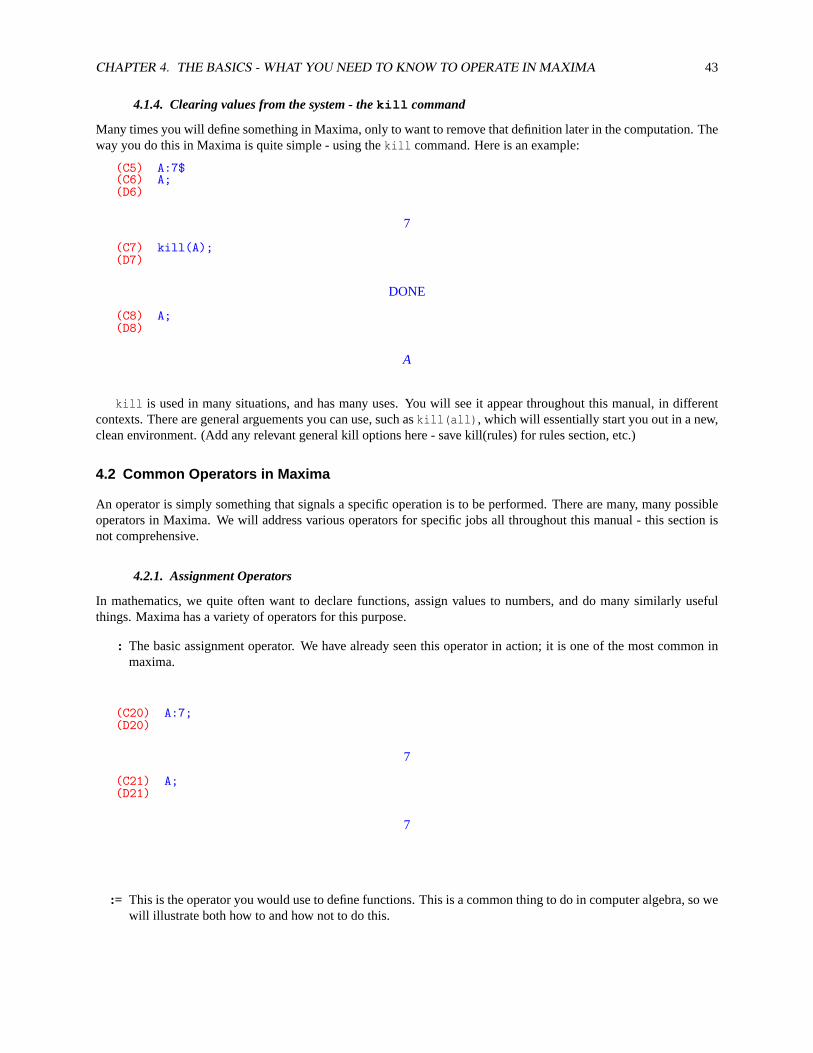
4.1.4. Clearing values from the system - thekill command
Many times you will define something in Maxima, only to want to remove that definition later in the computation. Theway you do this in Maxima is quite simple - using thekill command. Here is an example:
(C5) A:7$(C6) A;(D6)
7
(C7) kill(A);(D7)
DONE
(C8) A;(D8)
A
kill is used in many situations, and has many uses. You will see it appear throughout this manual, in differentcontexts. There are general arguements you can use, such askill(all), which will essentially start you out in a new,clean environment. (Add any relevant general kill options here - save kill(rules) for rules section, etc.)
4.2 Common Operators in Maxima
An operator is simply something that signals a specific operation is to be performed. There are many, many possibleoperators in Maxima. We will address various operators for specific jobs all throughout this manual - this section isnot comprehensive.
4.2.1. Assignment Operators
In mathematics, we quite often want to declare functions, assign values to numbers, and do many similarly usefulthings. Maxima has a variety of operators for this purpose.
: The basic assignment operator. We have already seen this operator in action; it is one of the most common inmaxima.
(C20) A:7;(D20)
7
(C21) A;(D21)
7
:= This is the operator you would use to define functions. This is a common thing to do in computer algebra, so wewill illustrate both how to and how not to do this.
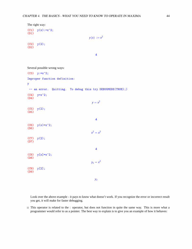
CHAPTER 4. THE BASICS - WHAT YOU NEED TO KNOW TO OPERATE IN MAXIMA 44
The right way:
(C1) y(x):=x^2;(D1)
y(x) := x2
(C2) y(2);(D2)
4
Several possible wrong ways:
(C3) y:=x^2;
Improper function definition:
y
-- an error. Quitting. To debug this try DEBUGMODE(TRUE);)
(C4) y=x^2;(D4)
y = x2
(C5) y(2);(D5)
4
(C6) y(x)=x^2;(D6)
x2 = x2
(C7) y(2);(D7)
4
(C8) y[x]=x^2;(D8)
yx = x2
(C9) y[2];(D9)
y2
Look over the above example - it pays to know what doesn’t work. If you recognize the error or incorrect resultyou get, it will make for faster debugging.
:: This operator is related to the : operator, but does not function in quite the same way. This is more what aprogrammer would refer to as a pointer. The best way to explain is to give you an example of how it behaves:
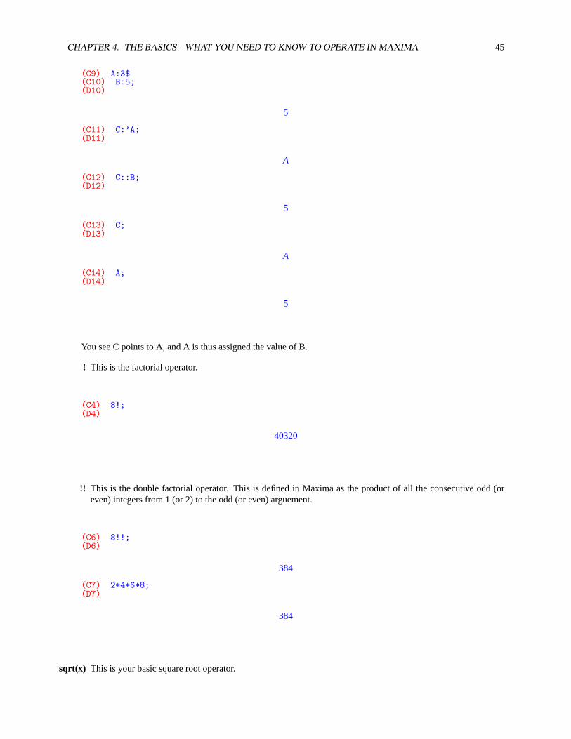
CHAPTER 4. THE BASICS - WHAT YOU NEED TO KNOW TO OPERATE IN MAXIMA 45
(C9) A:3$(C10) B:5;(D10)
5
(C11) C:’A;(D11)
A
(C12) C::B;(D12)
5
(C13) C;(D13)
A
(C14) A;(D14)
5
You see C points to A, and A is thus assigned the value of B.
! This is the factorial operator.
(C4) 8!;(D4)
40320
!! This is the double factorial operator. This is defined in Maxima as the product of all the consecutive odd (oreven) integers from 1 (or 2) to the odd (or even) arguement.
(C6) 8!!;(D6)
384
(C7) 2*4*6*8;(D7)
384
sqrt(x) This is your basic square root operator.
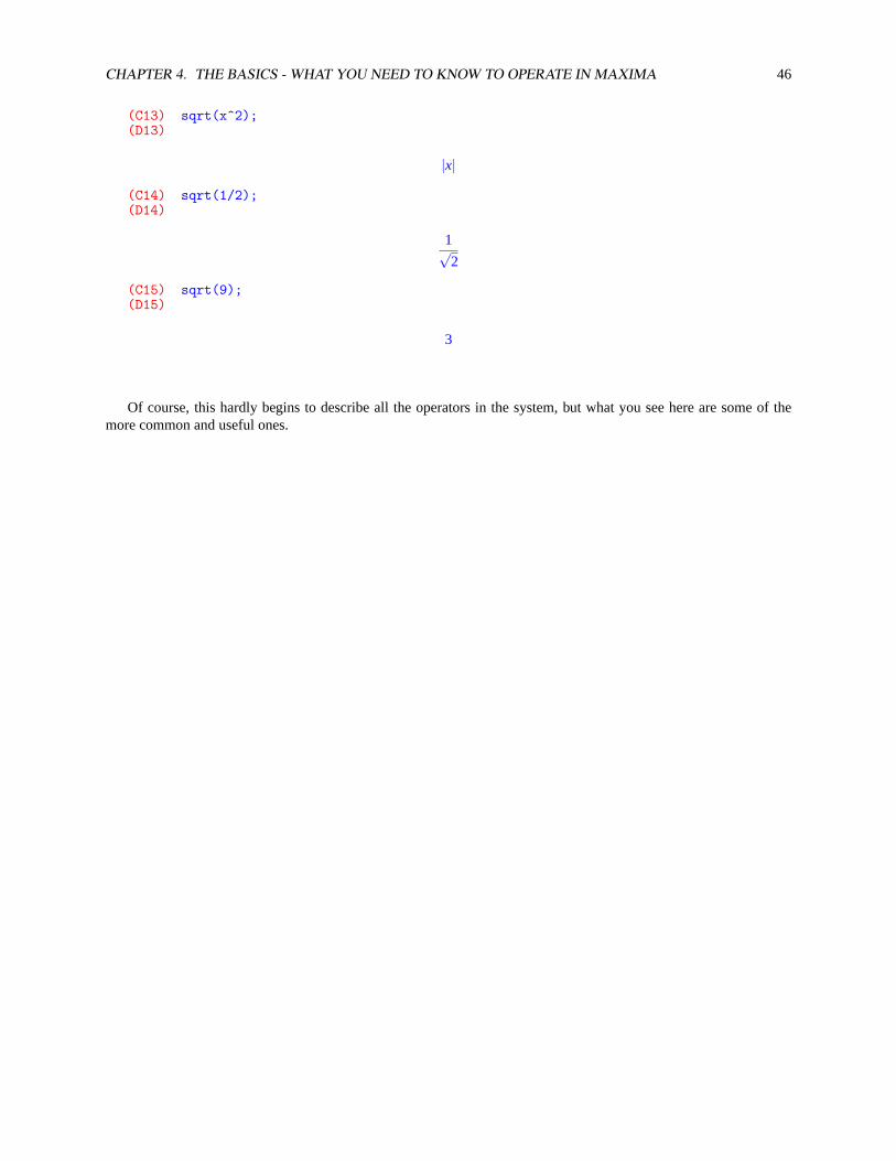
CHAPTER 4. THE BASICS - WHAT YOU NEED TO KNOW TO OPERATE IN MAXIMA 46
(C13) sqrt(x^2);(D13)
|x|
(C14) sqrt(1/2);(D14)
1√2
(C15) sqrt(9);(D15)
3
Of course, this hardly begins to describe all the operators in the system, but what you see here are some of themore common and useful ones.
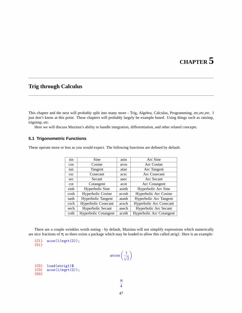
CHAPTER 5
Trig through Calculus
This chapter and the next will probably split into many more - Trig, Algebra, Calculus, Programming, etc,etc,etc. Ijust don’t know at this point. These chapters will probably largely be example based. Using things such as ratsimp,trigsimp, etc.
Here we will discuss Maxima’s ability to handle integration, differentiation, and other related concepts.
5.1 Trigonometric Functions
These operate more or less as you would expect. The following functions are defined by default:
sin Sine asin Arc Sinecos Cosine acos Arc Cosinetan Tangent atan Arc Tangentcsc Cosecant acsc Arc Cosecantsec Secant asec Arc Secantcot Cotangent acot Arc Cotangentsinh Hyperbolic Sine asinh Hyperbolic Arc Sinecosh Hyperbolic Cosine acosh Hyperbolic Arc Cosinetanh Hyperbolic Tangent atanh Hyperbolic Arc Tangentcsch Hyperbolic Cosecant acsch Hyperbolic Arc Cosecantsech Hyperbolic Secant asech Hyperbolic Arc Secantcoth Hyperbolic Cotangent acoth Hyperbolic Arc Cotangent
There are a couple wrinkles worth noting - by default, Maxima will not simplify expressions which numericallyare nice fractions ofπ, so there exists a package which may be loaded to allow this called atrig1. Here is an example:
(C1) acos(1/sqrt(2));(D1)
arccos
(1√2
)(C2) load(atrig1)$(C3) acos(1/sqrt(2));(D3)
π4
47
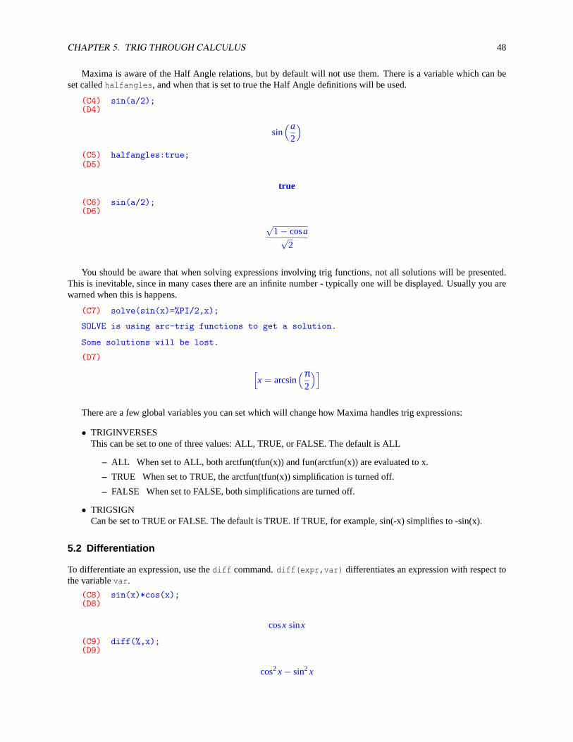
CHAPTER 5. TRIG THROUGH CALCULUS 48
Maxima is aware of the Half Angle relations, but by default will not use them. There is a variable which can beset calledhalfangles, and when that is set to true the Half Angle definitions will be used.
(C4) sin(a/2);(D4)
sin(a
2
)(C5) halfangles:true;(D5)
true
(C6) sin(a/2);(D6)
√1− cosa√
2
You should be aware that when solving expressions involving trig functions, not all solutions will be presented.This is inevitable, since in many cases there are an infinite number - typically one will be displayed. Usually you arewarned when this is happens.
(C7) solve(sin(x)=%PI/2,x);
SOLVE is using arc-trig functions to get a solution.
Some solutions will be lost.
(D7) [x = arcsin
(π2
)]There are a few global variables you can set which will change how Maxima handles trig expressions:
• TRIGINVERSESThis can be set to one of three values: ALL, TRUE, or FALSE. The default is ALL
– ALL When set to ALL, both arctfun(tfun(x)) and fun(arctfun(x)) are evaluated to x.
– TRUE When set to TRUE, the arctfun(tfun(x)) simplification is turned off.
– FALSE When set to FALSE, both simplifications are turned off.
• TRIGSIGNCan be set to TRUE or FALSE. The default is TRUE. If TRUE, for example, sin(-x) simplifies to -sin(x).
5.2 Differentiation
To differentiate an expression, use thediff command.diff(expr,var) differentiates an expression with respect tothe variablevar.
(C8) sin(x)*cos(x);(D8)
cosx sinx
(C9) diff(%,x);(D9)
cos2x− sin2x
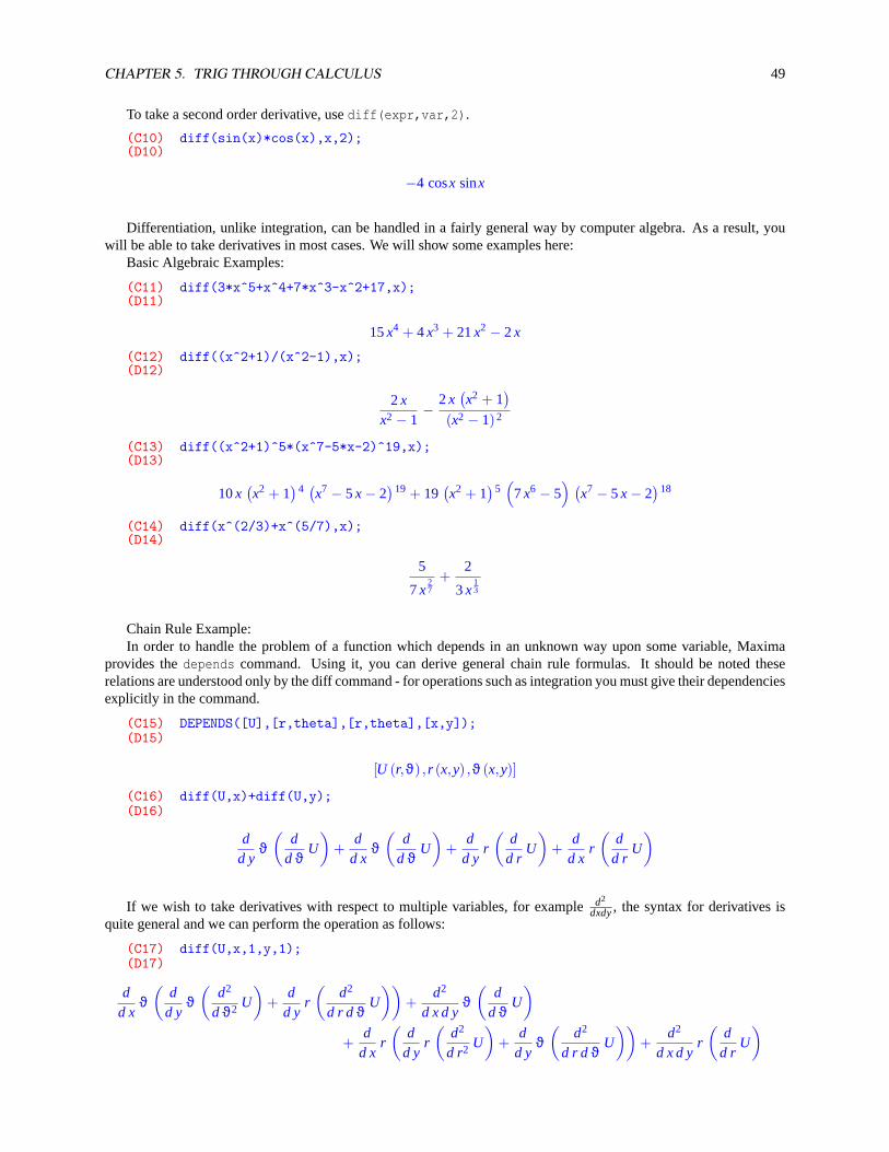
CHAPTER 5. TRIG THROUGH CALCULUS 49
To take a second order derivative, usediff(expr,var,2).
(C10) diff(sin(x)*cos(x),x,2);(D10)
−4 cosx sinx
Differentiation, unlike integration, can be handled in a fairly general way by computer algebra. As a result, youwill be able to take derivatives in most cases. We will show some examples here:
Basic Algebraic Examples:
(C11) diff(3*x^5+x^4+7*x^3-x^2+17,x);(D11)
15x4 + 4x3 + 21x2 − 2x
(C12) diff((x^2+1)/(x^2-1),x);(D12)
2xx2 − 1
−2x(x2 + 1
)(x2 − 1)2
(C13) diff((x^2+1)^5*(x^7-5*x-2)^19,x);(D13)
10x(x2 + 1
)4 (x7 − 5x− 2)19 + 19
(x2 + 1
)5(
7x6 − 5) (
x7 − 5x− 2)18
(C14) diff(x^(2/3)+x^(5/7),x);(D14)
5
7x27
+2
3x13
Chain Rule Example:In order to handle the problem of a function which depends in an unknown way upon some variable, Maxima
provides thedepends command. Using it, you can derive general chain rule formulas. It should be noted theserelations are understood only by the diff command - for operations such as integration you must give their dependenciesexplicitly in the command.
(C15) DEPENDS([U],[r,theta],[r,theta],[x,y]);(D15)
[U (r,ϑ) , r (x,y) ,ϑ(x,y)]
(C16) diff(U,x)+diff(U,y);(D16)
dd y
ϑ(
dd ϑ
U
)+
dd x
ϑ(
dd ϑ
U
)+
dd y
r
(d
d rU
)+
dd x
r
(d
d rU
)
If we wish to take derivatives with respect to multiple variables, for exampled2
dxdy, the syntax for derivatives isquite general and we can perform the operation as follows:
(C17) diff(U,x,1,y,1);(D17)
dd x
ϑ(
dd y
ϑ(
d2
d ϑ2 U
)+
dd y
r
(d2
d r d ϑU
))+
d2
d x d yϑ(
dd ϑ
U
)+
dd x
r
(d
d yr
(d2
d r2 U
)+
dd y
ϑ(
d2
d r d ϑU
))+
d2
d x d yr
(d
d rU
)

CHAPTER 5. TRIG THROUGH CALCULUS 50
This is the same thing as doing
(C18) diff(diff(U,x),y);(D18)
dd x
ϑ(
dd y
ϑ(
d2
d ϑ2 U
)+
dd y
r
(d2
d r d ϑU
))+
d2
d x d yϑ(
dd ϑ
U
)+
dd x
r
(d
d yr
(d2
d r2 U
)+
dd y
ϑ(
d2
d r d ϑU
))+
d2
d x d yr
(d
d rU
)
Trigonometric Derivatives:
(C25) diff(cos(x),x);(D25)
−sinx
(C26) diff(acos(x),x);(D26)
− 1√1− x2
(C27) diff(tan(x),x);(D27)
sec2x
(C28) diff(atan(x),x);(D28)
1x2 + 1
(C29) diff(sinh(x),x);(D29)
coshx
(C30) diff(asinh(x),x);(D30)
1√x2 + 1
5.3 Integration
Unlike differentiation, integration cannot be readily expressed in a general way. Maxima is quite capable when itcomes to to such problems, although like all computer algebra systems it has its limits.
In general,integrate is the command most users will use to perform various types of basic integrals. It istherefore a logical place to begin the introduction.
Beginning with a very basic example:
(C31) integrate(a*x^n,x);
Is n+1 zero or nonzero?
nonzero;
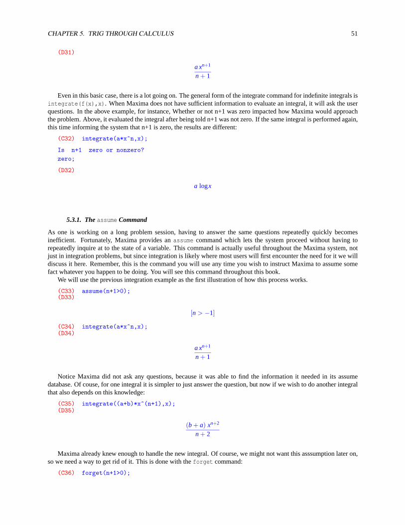
CHAPTER 5. TRIG THROUGH CALCULUS 51
(D31)
a xn+1
n + 1
Even in this basic case, there is a lot going on. The general form of the integrate command for indefinite integrals isintegrate(f(x),x). When Maxima does not have sufficient information to evaluate an integral, it will ask the userquestions. In the above example, for instance, Whether or not n+1 was zero impacted how Maxima would approachthe problem. Above, it evaluated the integral after being told n+1 was not zero. If the same integral is performed again,this time informing the system that n+1 is zero, the results are different:
(C32) integrate(a*x^n,x);
Is n+1 zero or nonzero?
zero;
(D32)
a logx
5.3.1. Theassume Command
As one is working on a long problem session, having to answer the same questions repeatedly quickly becomesinefficient. Fortunately, Maxima provides anassume command which lets the system proceed without having torepeatedly inquire at to the state of a variable. This command is actually useful throughout the Maxima system, notjust in integration problems, but since integration is likely where most users will first encounter the need for it we willdiscuss it here. Remember, this is the command you will use any time you wish to instruct Maxima to assume somefact whatever you happen to be doing. You will see this command throughout this book.
We will use the previous integration example as the first illustration of how this process works.
(C33) assume(n+1>0);(D33)
[n > −1]
(C34) integrate(a*x^n,x);(D34)
a xn+1
n + 1
Notice Maxima did not ask any questions, because it was able to find the information it needed in its assumedatabase. Of couse, for one integral it is simpler to just answer the question, but now if we wish to do another integralthat also depends on this knowledge:
(C35) integrate((a+b)*x^(n+1),x);(D35)
(b + a) xn+2
n + 2
Maxima already knew enough to handle the new integral. Of course, we might not want this asssumption later on,so we need a way to get rid of it. This is done with theforget command:
(C36) forget(n+1>0);
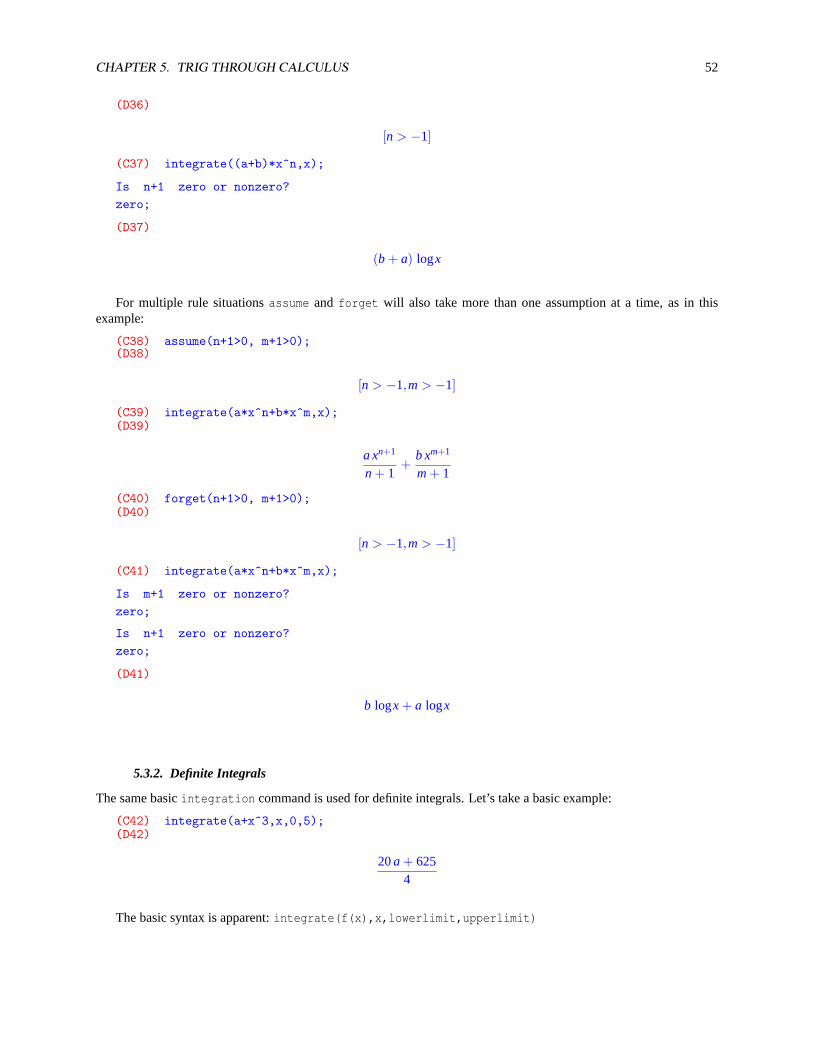
CHAPTER 5. TRIG THROUGH CALCULUS 52
(D36)
[n > −1]
(C37) integrate((a+b)*x^n,x);
Is n+1 zero or nonzero?
zero;
(D37)
(b + a) logx
For multiple rule situationsassume andforget will also take more than one assumption at a time, as in thisexample:
(C38) assume(n+1>0, m+1>0);(D38)
[n > −1,m > −1]
(C39) integrate(a*x^n+b*x^m,x);(D39)
a xn+1
n + 1+
b xm+1
m+ 1
(C40) forget(n+1>0, m+1>0);(D40)
[n > −1,m > −1]
(C41) integrate(a*x^n+b*x^m,x);
Is m+1 zero or nonzero?
zero;
Is n+1 zero or nonzero?
zero;
(D41)
b logx + a logx
5.3.2. Definite Integrals
The same basicintegration command is used for definite integrals. Let’s take a basic example:
(C42) integrate(a+x^3,x,0,5);(D42)
20a + 6254
The basic syntax is apparent:integrate(f(x),x,lowerlimit,upperlimit)
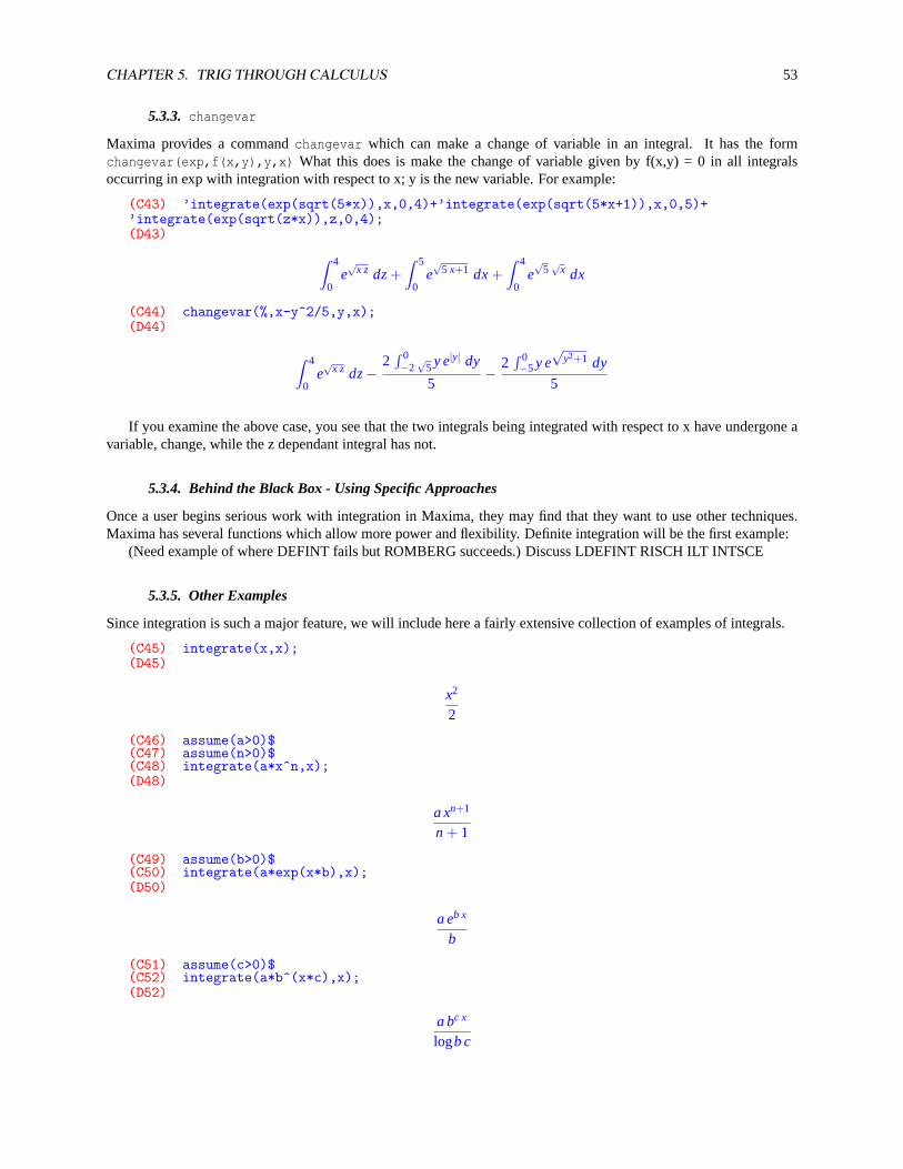
CHAPTER 5. TRIG THROUGH CALCULUS 53
5.3.3. changevar
Maxima provides a commandchangevar which can make a change of variable in an integral. It has the formchangevar(exp,f(x,y),y,x) What this does is make the change of variable given by f(x,y) = 0 in all integralsoccurring in exp with integration with respect to x; y is the new variable. For example:
(C43) ’integrate(exp(sqrt(5*x)),x,0,4)+’integrate(exp(sqrt(5*x+1)),x,0,5)+’integrate(exp(sqrt(z*x)),z,0,4);(D43) Z 4
0e√
x z dz+Z 5
0e√
5 x+1 dx+Z 4
0e√
5√
x dx
(C44) changevar(%,x-y^2/5,y,x);(D44)
Z 4
0e√
x z dz−2
R 0−2
√5y e|y| dy
5−
2R 0−5y e
√y2+1 dy
5
If you examine the above case, you see that the two integrals being integrated with respect to x have undergone avariable, change, while the z dependant integral has not.
5.3.4. Behind the Black Box - Using Specific Approaches
Once a user begins serious work with integration in Maxima, they may find that they want to use other techniques.Maxima has several functions which allow more power and flexibility. Definite integration will be the first example:
(Need example of where DEFINT fails but ROMBERG succeeds.) Discuss LDEFINT RISCH ILT INTSCE
5.3.5. Other Examples
Since integration is such a major feature, we will include here a fairly extensive collection of examples of integrals.
(C45) integrate(x,x);(D45)
x2
2
(C46) assume(a>0)$(C47) assume(n>0)$(C48) integrate(a*x^n,x);(D48)
a xn+1
n + 1
(C49) assume(b>0)$(C50) integrate(a*exp(x*b),x);(D50)
a eb x
b
(C51) assume(c>0)$(C52) integrate(a*b^(x*c),x);(D52)
a bc x
logb c
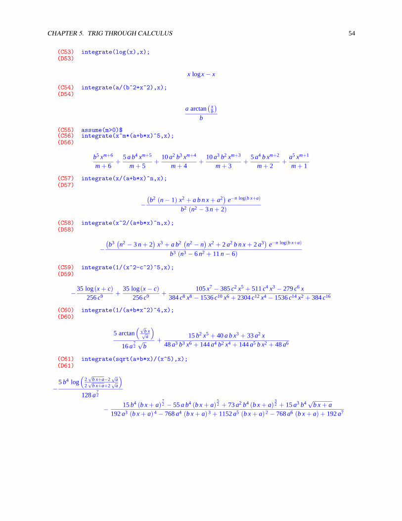
CHAPTER 5. TRIG THROUGH CALCULUS 54
(C53) integrate(log(x),x);(D53)
x logx− x
(C54) integrate(a/(b^2+x^2),x);(D54)
a arctan(
xb
)b
(C55) assume(m>0)$(C56) integrate(x^m*(a+b*x)^5,x);(D56)
b5 xm+6
m+ 6+
5a b4 xm+5
m+ 5+
10a2 b3 xm+4
m+ 4+
10a3 b2 xm+3
m+ 3+
5a4 b xm+2
m+ 2+
a5 xm+1
m+ 1
(C57) integrate(x/(a+b*x)^n,x);(D57)
−(b2 (n− 1) x2 + a b n x+ a2
)e−n log(b x+a)
b2 (n2 − 3n + 2)
(C58) integrate(x^2/(a+b*x)^n,x);(D58)
−(b3(n2 − 3n + 2
)x3 + a b2
(n2 − n
)x2 + 2a2 b n x+ 2a3
)e−n log(b x+a)
b3 (n3 − 6n2 + 11n− 6)
(C59) integrate(1/(x^2-c^2)^5,x);(D59)
−35 log(x + c)256c9 +
35 log(x− c)256c9 +
105x7 − 385c2 x5 + 511c4 x3 − 279c6 x384c8 x8 − 1536c10 x6 + 2304c12 x4 − 1536c14 x2 + 384c16
(C60) integrate(1/(a+b*x^2)^4,x);(D60)
5 arctan(√
b x√a
)16a
72√
b+
15b2 x5 + 40a b x3 + 33a2 x48a3 b3 x6 + 144a4 b2 x4 + 144a5 b x2 + 48a6
(C61) integrate(sqrt(a+b*x)/(x^5),x);(D61)
−5b4 log
(2√
b x+a−2√
a2√
b x+a+2√
a
)128a
72
− 15b4 (b x+ a)72 − 55a b4 (b x+ a)
52 + 73a2 b4 (b x+ a)
32 + 15a3 b4
√b x+ a
192a3 (b x+ a)4 − 768a4 (b x+ a)3 + 1152a5 (b x+ a)2 − 768a6 (b x+ a) + 192a7
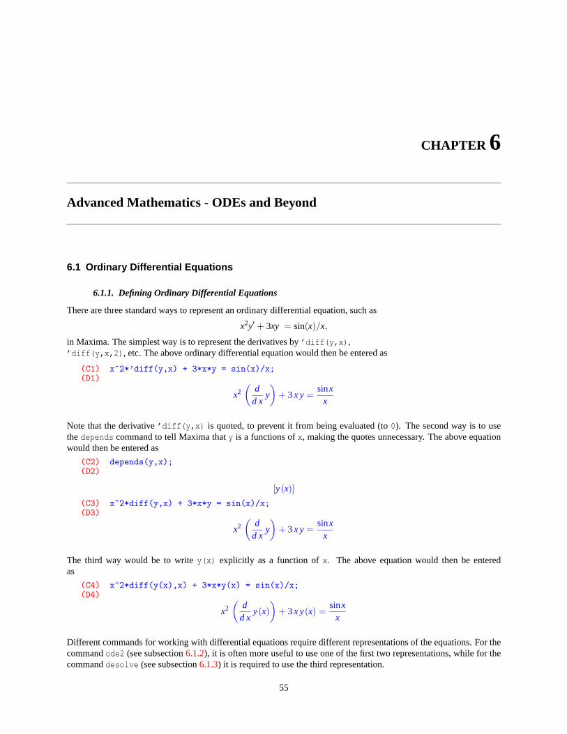
CHAPTER 6
Advanced Mathematics - ODEs and Beyond
6.1 Ordinary Differential Equations
6.1.1. Defining Ordinary Differential Equations
There are three standard ways to represent an ordinary differential equation, such as
x2y′ + 3xy = sin(x)/x,
in Maxima. The simplest way is to represent the derivatives by’diff(y,x),’diff(y,x,2), etc. The above ordinary differential equation would then be entered as
(C1) x^2*’diff(y,x) + 3*x*y = sin(x)/x;(D1)
x2(
dd x
y
)+ 3x y =
sinxx
Note that the derivative’diff(y,x) is quoted, to prevent it from being evaluated (to0). The second way is to usethedepends command to tell Maxima thaty is a functions ofx, making the quotes unnecessary. The above equationwould then be entered as
(C2) depends(y,x);(D2)
[y(x)]
(C3) x^2*diff(y,x) + 3*x*y = sin(x)/x;(D3)
x2(
dd x
y
)+ 3x y =
sinxx
The third way would be to writey(x) explicitly as a function ofx. The above equation would then be enteredas
(C4) x^2*diff(y(x),x) + 3*x*y(x) = sin(x)/x;(D4)
x2(
dd x
y(x))
+ 3x y(x) =sinx
x
Different commands for working with differential equations require different representations of the equations. For thecommandode2 (see subsection6.1.2), it is often more useful to use one of the first two representations, while for thecommanddesolve (see subsection6.1.3) it is required to use the third representation.
55
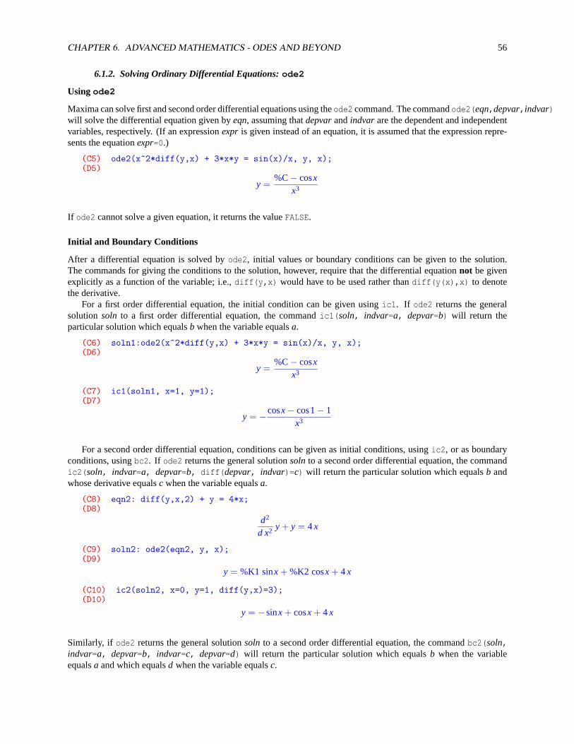
CHAPTER 6. ADVANCED MATHEMATICS - ODES AND BEYOND 56
6.1.2. Solving Ordinary Differential Equations:ode2
Usingode2
Maxima can solve first and second order differential equations using theode2 command. The commandode2(eqn,depvar,indvar)will solve the differential equation given byeqn, assuming thatdepvarandindvar are the dependent and independentvariables, respectively. (If an expressionexpr is given instead of an equation, it is assumed that the expression repre-sents the equationexpr=0.)
(C5) ode2(x^2*diff(y,x) + 3*x*y = sin(x)/x, y, x);(D5)
y =%C− cosx
x3
If ode2 cannot solve a given equation, it returns the valueFALSE.
Initial and Boundary Conditions
After a differential equation is solved byode2, initial values or boundary conditions can be given to the solution.The commands for giving the conditions to the solution, however, require that the differential equationnot be givenexplicitly as a function of the variable; i.e.,diff(y,x) would have to be used rather thandiff(y(x),x) to denotethe derivative.
For a first order differential equation, the initial condition can be given usingic1. If ode2 returns the generalsolution soln to a first order differential equation, the commandic1(soln, indvar=a, depvar=b) will return theparticular solution which equalsb when the variable equalsa.
(C6) soln1:ode2(x^2*diff(y,x) + 3*x*y = sin(x)/x, y, x);(D6)
y =%C− cosx
x3
(C7) ic1(soln1, x=1, y=1);(D7)
y = −cosx− cos1− 1x3
For a second order differential equation, conditions can be given as initial conditions, usingic2, or as boundaryconditions, usingbc2. If ode2 returns the general solutionsoln to a second order differential equation, the commandic2(soln, indvar=a, depvar=b, diff(depvar, indvar)=c) will return the particular solution which equalsb andwhose derivative equalsc when the variable equalsa.
(C8) eqn2: diff(y,x,2) + y = 4*x;(D8)
d2
d x2 y + y = 4x
(C9) soln2: ode2(eqn2, y, x);(D9)
y = %K1 sinx + %K2 cosx + 4x
(C10) ic2(soln2, x=0, y=1, diff(y,x)=3);(D10)
y = −sinx + cosx + 4x
Similarly, if ode2 returns the general solutionsoln to a second order differential equation, the commandbc2(soln,indvar=a, depvar=b, indvar=c, depvar=d) will return the particular solution which equalsb when the variableequalsa and which equalsd when the variable equalsc.
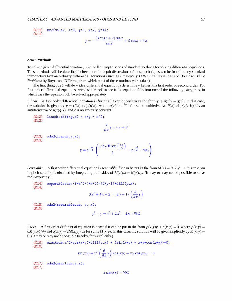
CHAPTER 6. ADVANCED MATHEMATICS - ODES AND BEYOND 57
(C11) bc2(soln2, x=0, y=3, x=2, y=1);(D11)
y = − (3 cos2+ 7) sinxsin2
+ 3 cosx + 4x
ode2 Methods
To solve a given differential equation,ode2 will attempt a series of standard methods for solving differential equations.These methods will be described below, more in-depth discussions of these techniques can be found in any standardintroductory text on ordinary differential equations (such asElementary Differential Equations and Boundary ValueProblems by Boyce and DiPrima, from which most of these routines were taken).
The first thingode2 will do with a differential equation is determine whether it is first order or second order. Forfirst order differential equations,ode2 will check to see if the equation falls into one of the following categories, inwhich case the equation will be solved appropriately.
Linear. A first order differential equation islinear if it can be written in the formy′ + p(x)y = q(x). In this case,the solution is given byy = (I(x)+c)/µ(x), whereµ(x) is eP(x) for some antiderivativeP(x) of p(x), I(x) is anantiderivative ofµ(x)q(x), andc is an arbitrary constant.
(C12) linode:diff(y,x) + x*y = x^2;(D12)
dd x
y + x y = x2
(C13) ode2(linode,y,x);(D13)
y = e−x22
√2√
π i erf(
i x√2
)2
+ x ex22 + %C
Separable. A first order differential equation isseparableif it can be put in the formM(x) = N(y)y′. In this case, animplicit solution is obtained by integrating both sides ofM(x)dx= N(y)dy. (It may or may not be possible to solvefor y explicitly.)
(C14) separableode:(3*x^2+4*x+2)=(2*y-1)*diff(y,x);(D14)
3x2 + 4x + 2 = (2y− 1)(
dd x
y
)(C15) ode2(separableode, y, x);(D15)
y2 − y = x3 + 2x2 + 2x + %C
Exact. A first order differential equation isexactif it can be put in the formp(x,y)y′ +q(x,y) = 0, wherep(x,y) =∂M(x,y)/∂y andq(x,y) = ∂M(x,y)/∂x for someM(x,y). In this case, the solution will be given implicitly byM(x,y) =0. (It may or may not be possible to solve fory explicitly.)
(C16) exactode:x^2*cos(x*y)*diff(y,x) + (sin(x*y) + x*y*cos(x*y))=0;(D16)
sin(x y) + x2(
dd x
y
)cos(x y) + x y cos(x y) = 0
(C17) ode2(exactode,y,x);(D17)
x sin(x y) = %C
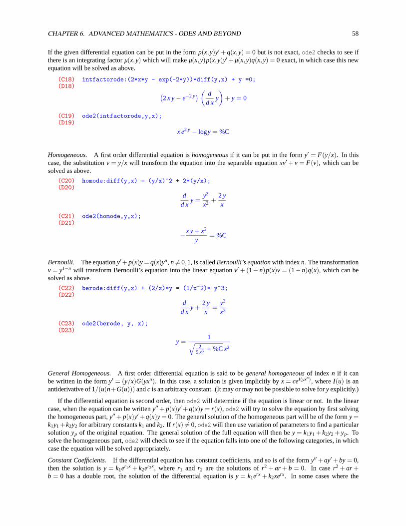
CHAPTER 6. ADVANCED MATHEMATICS - ODES AND BEYOND 58
If the given differential equation can be put in the formp(x,y)y′ +q(x,y) = 0 but is not exact,ode2 checks to see ifthere is an integrating factorµ(x,y) which will makeµ(x,y)p(x,y)y′+µ(x,y)q(x,y) = 0 exact, in which case this newequation will be solved as above.
(C18) intfactorode:(2*x*y - exp(-2*y))*diff(y,x) + y =0;(D18) (
2x y− e−2 y) ( dd x
y
)+ y = 0
(C19) ode2(intfactorode,y,x);(D19)
x e2 y − logy = %C
Homogeneous. A first order differential equation ishomogeneousif it can be put in the formy′ = F(y/x). In thiscase, the substitutionv = y/x will transform the equation into the separable equationxv′ + v = F(v), which can besolved as above.
(C20) homode:diff(y,x) = (y/x)^2 + 2*(y/x);(D20)
dd x
y =y2
x2 +2yx
(C21) ode2(homode,y,x);(D21)
−x y+ x2
y= %C
Bernoulli. The equationy′+ p(x)y= q(x)yn, n 6= 0,1, is calledBernoulli’s equationwith indexn. The transformationv = y1−n will transform Bernoulli’s equation into the linear equationv′ +(1−n)p(x)v = (1−n)q(x), which can besolved as above.
(C22) berode:diff(y,x) + (2/x)*y = (1/x^2)* y^3;(D22)
dd x
y +2yx
=y3
x2
(C23) ode2(berode, y, x);(D23)
y =1√
25 x5 + %Cx2
General Homogeneous.A first order differential equation is said to begeneral homogeneousof index n if it canbe written in the formy′ = (y/x)G(yxn). In this case, a solution is given implicitly byx = ceI(yxn), whereI(u) is anantiderivative of 1/(u(n+G(u))) andc is an arbitrary constant. (It may or may not be possible to solve fory explicitly.)
If the differential equation is second order, thenode2 will determine if the equation is linear or not. In the linearcase, when the equation can be writteny′′+ p(x)y′+q(x)y = r(x), ode2 will try to solve the equation by first solvingthe homogeneous part,y′′+ p(x)y′+q(x)y = 0. The general solution of the homogeneous part will be of the formy =k1y1+k2y2 for arbitrary constantsk1 andk2. If r(x) 6= 0,ode2 will then use variation of parameters to find a particularsolutionyp of the original equation. The general solution of the full equation will then bey = k1y1 + k2y2 + yp. Tosolve the homogeneous part,ode2 will check to see if the equation falls into one of the following categories, in whichcase the equation will be solved appropriately.
Constant Coefficients.If the differential equation has constant coefficients, and so is of the formy′′ +ay′ +by= 0,then the solution isy = k1er1x + k2er2x, wherer1 and r2 are the solutions ofr2 + ar + b = 0. In caser2 + ar +b = 0 has a double root, the solution of the differential equation isy = k1erx + k2xerx. In some cases where the

CHAPTER 6. ADVANCED MATHEMATICS - ODES AND BEYOND 59
equation doesn’t have constant coefficients,ode2 will attempt to use a simple transformation to reduce it to constantcoefficents.
(C24) ccode1: diff(y,x,2) - 3*diff(y,x) + 2*y=0;(D24)
d2
d x2 y− 3
(d
d xy
)+ 2y = 0
(C25) ccode2: diff(y,x,2) - 4*diff(y,x) + 4*y=0;(D25)
d2
d x2 y− 4
(d
d xy
)+ 4y = 0
(C26) ode2(ccode1, y, x);(D26)
y = %K1e2 x + %K2ex
(C27) ode2(ccode2, y, x);(D27)
y = (%K2x + %K1) e2 x
Exact. A second order differential equation isexactif it can be written in the form[ f (x)y′]′+[g(x)y]′ = 0. Integratingthis equation will reduce it to a first order differential equation, which can be solved as above.
(C28) exactode2: x^2*diff(y,x,2) + x*diff(y,x) - y =0;(D28)
x2(
d2
d x2 y
)+ x
(d
d xy
)− y = 0
(C29) ode2(exactode2, y,x);(D29)
y = %K2x− %K12x
Euler. The equationx2y′′ + axy′ + by= 0 is Euler’s equation. The solution is given byy = k1xr1 + k2xr2, wherer1
andr2 are solutions ofr(r−1)+ar+b= 0. In caser(r−1)+ar+b= 0 has a double root, the solution is given byy=k1xr +k2 ln(x)xr .
(C30) eulerode1: x^2*diff(y,x,2) + 4*x*diff(y,x) + 2*y = 0;(D30)
x2(
d2
d x2 y
)+ 4x
(d
d xy
)+ 2y = 0
(C31) eulerode2: x^2*diff(y,x,2) + 5*x*diff(y,x) + 4*y = 0;(D31)
x2(
d2
d x2 y
)+ 5x
(d
d xy
)+ 4y = 0
(C32) ode2(eulerode1, y, x);(D32)
y =%K1
x+
%K2x2
(C33) ode2(eulerode2, y, x);(D33)
y =%K2 logx + %K1
x2
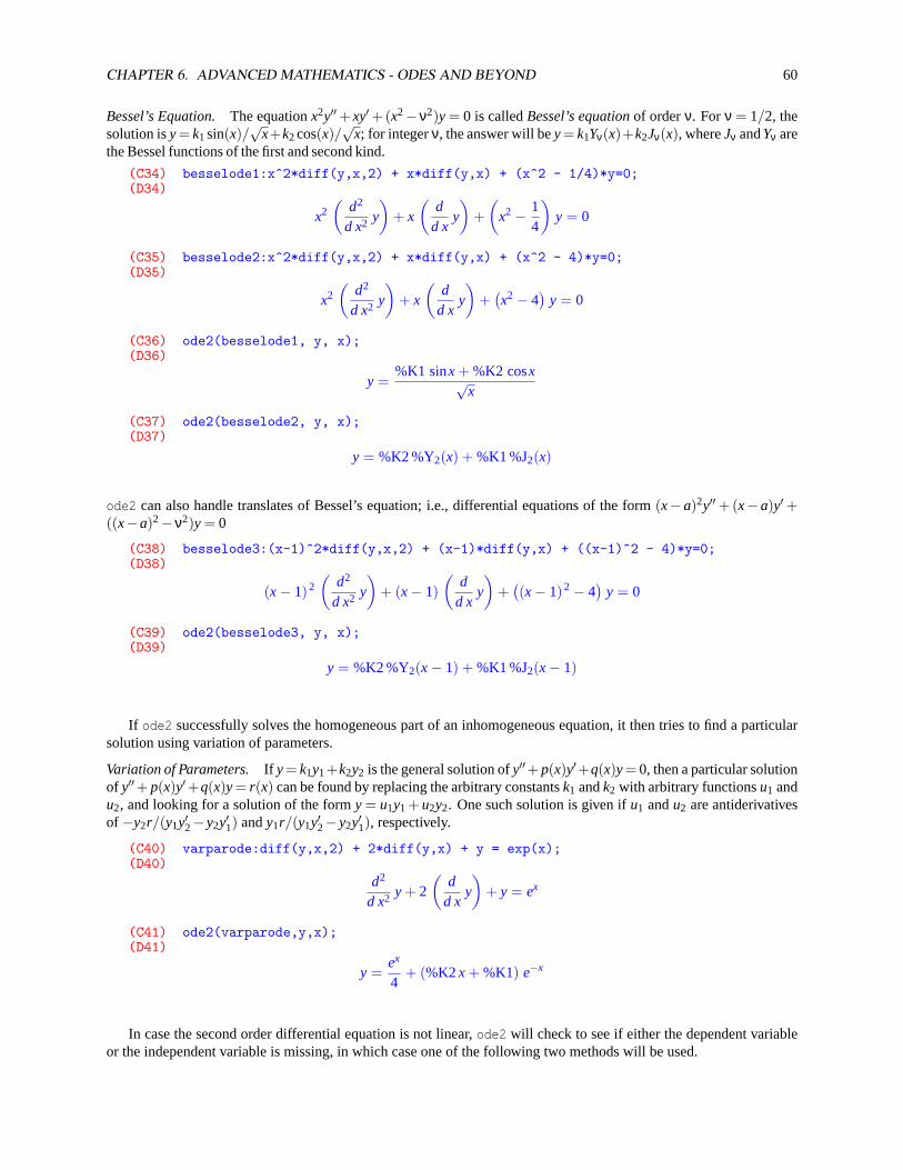
CHAPTER 6. ADVANCED MATHEMATICS - ODES AND BEYOND 60
Bessel’s Equation. The equationx2y′′+xy′+(x2−ν2)y = 0 is calledBessel’s equationof orderν. Forν = 1/2, thesolution isy= k1sin(x)/
√x+k2cos(x)/
√x; for integerν, the answer will bey= k1Yν(x)+k2Jν(x), whereJν andYν are
the Bessel functions of the first and second kind.
(C34) besselode1:x^2*diff(y,x,2) + x*diff(y,x) + (x^2 - 1/4)*y=0;(D34)
x2(
d2
d x2 y
)+ x
(d
d xy
)+(
x2 − 14
)y = 0
(C35) besselode2:x^2*diff(y,x,2) + x*diff(y,x) + (x^2 - 4)*y=0;(D35)
x2(
d2
d x2 y
)+ x
(d
d xy
)+(x2 − 4
)y = 0
(C36) ode2(besselode1, y, x);(D36)
y =%K1 sinx + %K2 cosx√
x
(C37) ode2(besselode2, y, x);(D37)
y = %K2 %Y2(x) + %K1 %J2(x)
ode2 can also handle translates of Bessel’s equation; i.e., differential equations of the form(x−a)2y′′ +(x−a)y′ +((x−a)2−ν2)y = 0
(C38) besselode3:(x-1)^2*diff(y,x,2) + (x-1)*diff(y,x) + ((x-1)^2 - 4)*y=0;(D38)
(x− 1)2(
d2
d x2 y
)+ (x− 1)
(d
d xy
)+((x− 1)2 − 4
)y = 0
(C39) ode2(besselode3, y, x);(D39)
y = %K2 %Y2(x− 1) + %K1 %J2(x− 1)
If ode2 successfully solves the homogeneous part of an inhomogeneous equation, it then tries to find a particularsolution using variation of parameters.
Variation of Parameters. If y= k1y1+k2y2 is the general solution ofy′′+ p(x)y′+q(x)y= 0, then a particular solutionof y′′+ p(x)y′+q(x)y= r(x) can be found by replacing the arbitrary constantsk1 andk2 with arbitrary functionsu1 andu2, and looking for a solution of the formy = u1y1 +u2y2. One such solution is given ifu1 andu2 are antiderivativesof −y2r/(y1y′2−y2y′1) andy1r/(y1y′2−y2y′1), respectively.
(C40) varparode:diff(y,x,2) + 2*diff(y,x) + y = exp(x);(D40)
d2
d x2 y + 2
(d
d xy
)+ y = ex
(C41) ode2(varparode,y,x);(D41)
y =ex
4+ (%K2x + %K1) e−x
In case the second order differential equation is not linear,ode2 will check to see if either the dependent variableor the independent variable is missing, in which case one of the following two methods will be used.
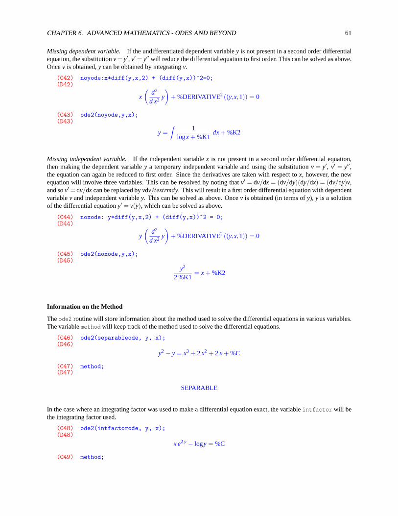
CHAPTER 6. ADVANCED MATHEMATICS - ODES AND BEYOND 61
Missing dependent variable.If the undifferentiated dependent variabley is not present in a second order differentialequation, the substitutionv= y′, v′ = y′′ will reduce the differential equation to first order. This can be solved as above.Oncev is obtained,y can be obtained by integratingv.
(C42) noyode:x*diff(y,x,2) + (diff(y,x))^2=0;(D42)
x
(d2
d x2 y
)+ %DERIVATIVE2 ((y,x,1)) = 0
(C43) ode2(noyode,y,x);(D43)
y =Z
1logx + %K1
dx+ %K2
Missing independent variable.If the independent variablex is not present in a second order differential equation,then making the dependent variabley a temporary independent variable and using the substitutionv = y′, v′ = y′′,the equation can again be reduced to first order. Since the derivatives are taken with respect tox, however, the newequation will involve three variables. This can be resolved by noting thatv′ = dv/dx = (dv/dy)(dy/dx) = (dv/dy)v,and sov′ = dv/dx can be replaced byvdv/textrmdy. This will result in a first order differential equation with dependentvariablev and independent variabley. This can be solved as above. Oncev is obtained (in terms ofy), y is a solutionof the differential equationy′ = v(y), which can be solved as above.
(C44) noxode: y*diff(y,x,2) + (diff(y,x))^2 = 0;(D44)
y
(d2
d x2 y
)+ %DERIVATIVE2 ((y,x,1)) = 0
(C45) ode2(noxode,y,x);(D45)
y2
2 %K1= x + %K2
Information on the Method
Theode2 routine will store information about the method used to solve the differential equations in various variables.The variablemethod will keep track of the method used to solve the differential equations.
(C46) ode2(separableode, y, x);(D46)
y2 − y = x3 + 2x2 + 2x + %C
(C47) method;(D47)
SEPARABLE
In the case where an integrating factor was used to make a differential equation exact, the variableintfactor will bethe integrating factor used.
(C48) ode2(intfactorode, y, x);(D48)
x e2 y − logy = %C
(C49) method;
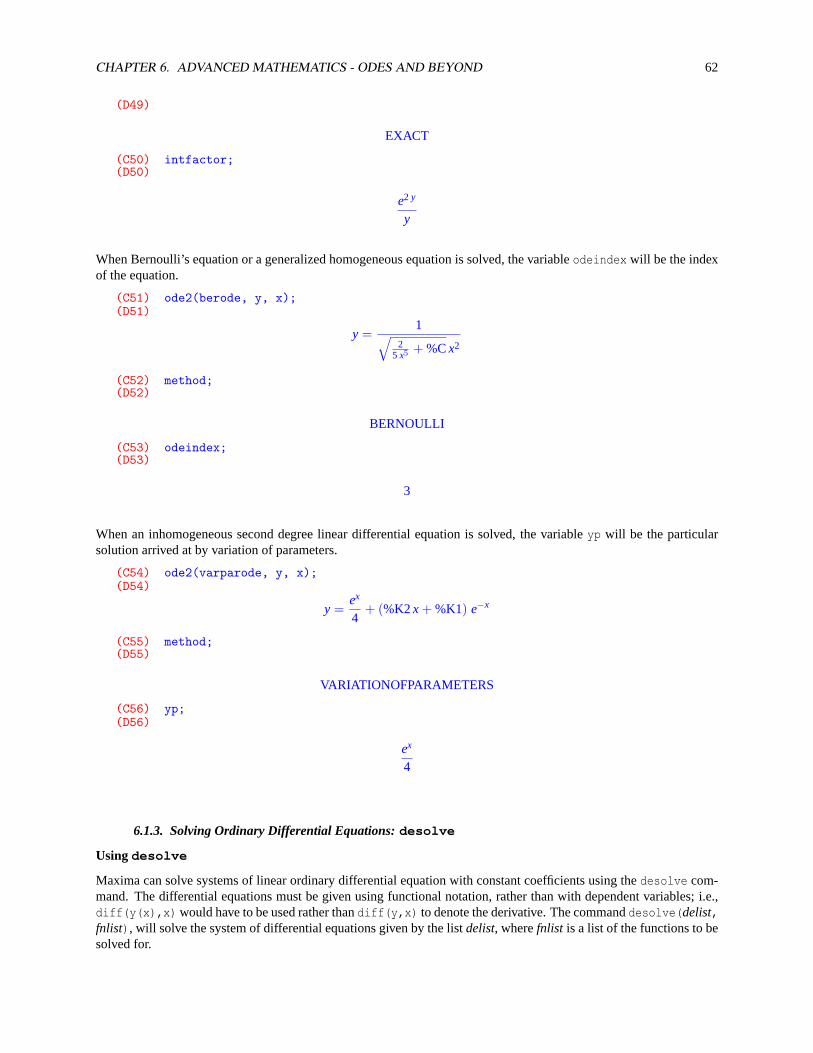
CHAPTER 6. ADVANCED MATHEMATICS - ODES AND BEYOND 62
(D49)
EXACT
(C50) intfactor;(D50)
e2 y
y
When Bernoulli’s equation or a generalized homogeneous equation is solved, the variableodeindex will be the indexof the equation.
(C51) ode2(berode, y, x);(D51)
y =1√
25 x5 + %Cx2
(C52) method;(D52)
BERNOULLI
(C53) odeindex;(D53)
3
When an inhomogeneous second degree linear differential equation is solved, the variableyp will be the particularsolution arrived at by variation of parameters.
(C54) ode2(varparode, y, x);(D54)
y =ex
4+ (%K2x + %K1) e−x
(C55) method;(D55)
VARIATIONOFPARAMETERS
(C56) yp;(D56)
ex
4
6.1.3. Solving Ordinary Differential Equations:desolve
Usingdesolve
Maxima can solve systems of linear ordinary differential equation with constant coefficients using thedesolve com-mand. The differential equations must be given using functional notation, rather than with dependent variables; i.e.,diff(y(x),x) would have to be used rather thandiff(y,x) to denote the derivative. The commanddesolve(delist,fnlist), will solve the system of differential equations given by the listdelist, wherefnlist is a list of the functions to besolved for.
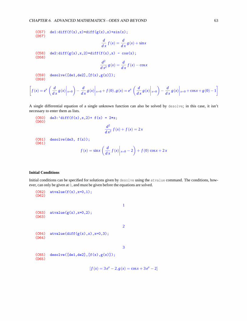
CHAPTER 6. ADVANCED MATHEMATICS - ODES AND BEYOND 63
(C57) de1:diff(f(x),x)=diff(g(x),x)+sin(x);(D57)
dd x
f (x) =d
d xg(x) + sinx
(C58) de2:diff(g(x),x,2)=diff(f(x),x) - cos(x);(D58)
d2
d x2 g(x) =d
d xf (x)− cosx
(C59) desolve([de1,de2],[f(x),g(x)]);(D59)[
f (x) = ex(
dd x
g(x)∣∣∣∣ x=0
)− d
d xg(x)
∣∣∣∣ x=0 + f (0) ,g(x) = ex(
dd x
g(x)∣∣∣∣ x=0
)− d
d xg(x)
∣∣∣∣ x=0 + cosx+ g(0)−1
]
A single differential equation of a single unknown function can also be solved bydesolve; in this case, it isn’tnecessary to enter them as lists.
(C60) de3:’diff(f(x),x,2)+ f(x) = 2*x;(D60)
d2
d x2 f (x) + f (x) = 2x
(C61) desolve(de3, f(x));(D61)
f (x) = sinx
(d
d xf (x)
∣∣∣∣ x=0 − 2
)+ f (0) cosx + 2x
Initial Conditions
Initial conditions can be specified for solutions given bydesolve using theatvalue command. The conditions, how-ever, can only be given at0, and must be given before the equations are solved.
(C62) atvalue(f(x),x=0,1);(D62)
1
(C63) atvalue(g(x),x=0,2);(D63)
2
(C64) atvalue(diff(g(x),x),x=0,3);(D64)
3
(C65) desolve([de1,de2],[f(x),g(x)]);(D65)
[ f (x) = 3ex − 2,g(x) = cosx + 3ex − 2]

CHAPTER 6. ADVANCED MATHEMATICS - ODES AND BEYOND 64
desolve Method
The desolve routine uses the LaPlace transform to solve the systems of differential equations. Iff (t) is definedfor all t ≥ 0, then the LaPlace transform off is given byF(s) = L{ f (t)} =
R ∞0 e−st f (t)dt. The LaPlace transform
has the useful property that a derivative is transformed into multiplication by the variable; ifL{ f (t)} = F(s), thenL{ f ′(t)} = sF(s)− f (0). The LaPlace transform can thus transform a system of linear differential equations into asystem of ordinary equations. (Note, however, that the LaPlace transform will transform multiplication by a variableinto differentiation; ifL{ f (t)} = F(s), thenL{t f (t)} = −F ′(s). The original differential equations need to haveconstant coefficients to prevent this.) If this new system can be solved, the LaPlace tranform can be inverted to givesolutions of the original system of differential equations.

CHAPTER 7
Matrix Operations and Vectors
Maxima has many matrix capabilities. Unfortunately it’s vector handling at the time of this writing is not terriblyrobust, and the reader is cautioned to use it with care.
65
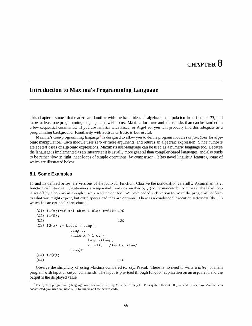
CHAPTER 8
Introduction to Maxima’s Programming Language
This chapter assumes that readers are familiar with the basic ideas of algebraic manipulation from Chapter??, andknow at least one programming language, and wish to use Maxima for more ambitious tasks than can be handled ina few sequential commands. If you are familiar with Pascal or Algol 60, you will probably find this adequate as aprogramming background. Familiarity with Fortran or Basic is less useful.
Maxima’s user-programming language1 is designed to allow you to define program modules orfunctionsfor alge-braic manipulation. Each module uses zero or more arguments, and returns an algebraic expression. Since numbersare special cases of algebraic expressions, Maxima’s user-language can be used as a numeric language too. Becausethe language is implemented as an interpreter it is usually more general than compiler-based languages, and also tendsto be rather slow in tight inner loops of simple operations, by comparison. It has novel linguistic features, some ofwhich are illustrated below.
8.1 Some Examples
f1 andf2 defined below, are versions of thefactorial function. Observe the punctuation carefully. Assignment is:,function definition is:=, statements are separated from one another by, (not terminatedby commas). The labelloopis set off by a comma as though it were a statement too. We have added indentation to make the programs conformto what you might expect, but extra spaces and tabs are optional. There is a conditional execution statement (theif)which has an optionalelse clause.
(C1) f1(x):=if x<1 then 1 else x*f1(x-1)$(C2) f1(5);(D2) 120(C3) f2(x) := block ([temp],
temp:1,while x > 1 do (
temp:x*temp,x:x-1), /*end while*/
temp)$(C4) f2(5);(D4) 120
Observe the simplicity of using Maxima compared to, say, Pascal. There is no need to write adriver or mainprogram with input or output commands. The input is provided through function application on an argument, and theoutput is the displayed value.
1The system-programming language used for implementing Maxima namely LISP, is quite different. If you wish to see how Maxima wasconstructed, you need to know LISP to understand the source code.
66
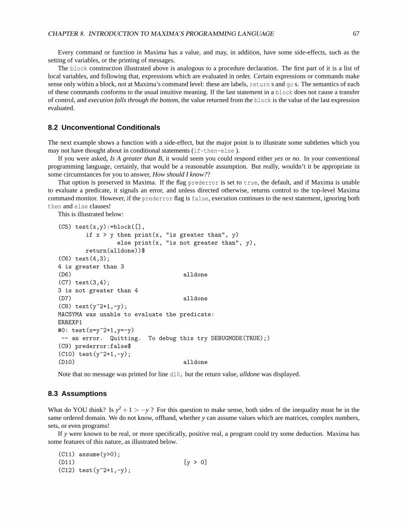
CHAPTER 8. INTRODUCTION TO MAXIMA’S PROGRAMMING LANGUAGE 67
Every command or function in Maxima has a value, and may, in addition, have some side-effects, such as thesetting of variables, or the printing of messages.
Theblock construction illustrated above is analogous to a procedure declaration. The first part of it is a list oflocal variables, and following that, expressions which are evaluated in order. Certain expressions or commands makesense only within a block, not at Maxima’s command level: these are labels,return s andgo s. The semantics of eachof these commands conforms to the usual intuitive meaning. If the last statement in ablock does not cause a transferof control, andexecution falls through the bottom, the value returned from theblock is the value of the last expressionevaluated.
8.2 Unconventional Conditionals
The next example shows a function with a side-effect, but the major point is to illustrate some subtleties which youmay not have thought about in conditional statements (if-then-else ).
If you were asked,Is A greater than B, it would seem you could respond eitheryesor no. In your conventionalprogramming language, certainly, that would be a reasonable assumption. But really, wouldn’t it be appropriate insome circumstances for you to answer,How should I know??
That option is preserved in Maxima. If the flagprederror is set totrue, the default, and if Maxima is unableto evaluate a predicate, it signals an error, and unless directed otherwise, returns control to the top-level Maximacommand monitor. However, if theprederror flag isfalse, execution continues to the next statement, ignoring boththen andelse clauses!
This is illustrated below:
(C5) test(x,y):=block([],if x > y then print(x, "is greater than", y)
else print(x, "is not greater than", y),return(alldone))$
(C6) test(4,3);4 is greater than 3(D6) alldone(C7) test(3,4);3 is not greater than 4(D7) alldone(C8) test(y^2+1,-y);MACSYMA was unable to evaluate the predicate:ERREXP1#0: test(x=y^2+1,y=-y)-- an error. Quitting. To debug this try DEBUGMODE(TRUE);)(C9) prederror:false$(C10) test(y^2+1,-y);(D10) alldone
Note that no message was printed for lined10, but the return value,alldonewas displayed.
8.3 Assumptions
What do YOU think? Isy2 + 1 > −y ? For this question to make sense, both sides of the inequality must be in thesame ordered domain. We do not know, offhand, whethery can assume values which are matrices, complex numbers,sets, or even programs!
If y were known to be real, or more specifically, positive real, a program could try some deduction. Maxima hassome features of this nature, as illustrated below.
(C11) assume(y>0);(D11) [y > 0](C12) test(y^2+1,-y);
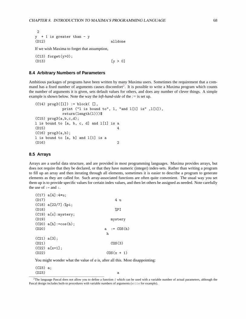
CHAPTER 8. INTRODUCTION TO MAXIMA’S PROGRAMMING LANGUAGE 68
2y + 1 is greater than - y(D12) alldone
If we wish Maxima to forget that assumption,
(C13) forget(y>0);(D13) [y > 0]
8.4 Arbitrary Numbers of Parameters
Ambitious packages of programs have been written by many Maxima users. Sometimes the requirement that a com-mand has a fixed number of arguments causes discomfort2. It is possible to write a Maxima program which countsthe number of arguments it is given, sets default values for others, and does any number of clever things. A simpleexample is shown below. Note the way theleft-hand-sideof the:= is set up.
(C14) prog3([l]) := block( [],print ("l is bound to", l, "and l[1] is" ,l[1]),return(length(l)))$
(C15) prog3(a,b,c,d);l is bound to [a, b, c, d] and l[1] is a(D15) 4(C16) prog3(a,b);l is bound to [a, b] and l[1] is a(D16) 2
8.5 Arrays
Arrays are a useful data structure, and are provided in most programming languages. Maxima provides arrays, butdoes not require that they be declared, or that they have numeric (integer) index-sets. Rather than writing a programto fill up an array and then iterating through all elements, sometimes it is easier to describe a program to generateelements as they are called for. Such array-associated functions are often quite convenient. The usual way you setthem up is to provide specific values for certain index values, and then let others be assigned as needed. Note carefullythe use of:= and:.
(C17) a[4]:4*u;(D17) 4 u(C18) a[22/7]:%pi;(D18) %PI(C19) a[x]:mystery;(D19) mystery(C20) a[h]:=cos(h);(D20) a := COS(h)
h(C21) a[3];(D21) COS(3)(C22) a[x+1];(D22) COS(x + 1)
You might wonder what the value ofa is, after all this. Most disappointing:
(C23) a;(D23) a
2The language Pascal does not allow you to define a functionf which can be used with a variable number of actual parameters, although thePascal design includes built-in procedures with variable numbers of arguments (write for example).
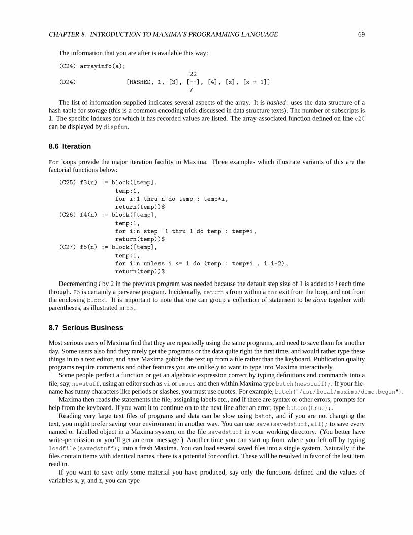
CHAPTER 8. INTRODUCTION TO MAXIMA’S PROGRAMMING LANGUAGE 69
The information that you are after is available this way:
(C24) arrayinfo(a);22
(D24) [HASHED, 1, [3], [--], [4], [x], [x + 1]]7
The list of information supplied indicates several aspects of the array. It ishashed: uses the data-structure of ahash-table for storage (this is a common encoding trick discussed in data structure texts). The number of subscripts is1. The specific indexes for which it has recorded values are listed. The array-associated function defined on linec20can be displayed bydispfun.
8.6 Iteration
For loops provide the major iteration facility in Maxima. Three examples which illustrate variants of this are thefactorial functions below:
(C25) f3(n) := block([temp],temp:1,for i:1 thru n do temp : temp*i,return(temp))$
(C26) f4(n) := block([temp],temp:1,for i:n step -1 thru 1 do temp : temp*i,return(temp))$
(C27) f5(n) := block([temp],temp:1,for i:n unless i <= 1 do (temp : temp*i , i:i-2),return(temp))$
Decrementingi by 2 in the previous program was needed because the default step size of 1 is added toi each timethrough.F5 is certainly a perverse program. Incidentally,return s from within afor exit from the loop, and not fromthe enclosingblock. It is important to note that one can group a collection of statement to bedonetogether withparentheses, as illustrated inf5.
8.7 Serious Business
Most serious users of Maxima find that they are repeatedly using the same programs, and need to save them for anotherday. Some users also find they rarely get the programs or the data quite right the first time, and would rather type thesethings in to a text editor, and have Maxima gobble the text up from a file rather than the keyboard. Publication qualityprograms require comments and other features you are unlikely to want to type into Maxima interactively.
Some people perfect a function or get an algebraic expression correct by typing definitions and commands into afile, say,newstuff, using an editor such asvi oremacs and then within Maxima typebatch(newstuff);. If your file-name has funny characters like periods or slashes, you must use quotes. For example,batch("/usr/local/maxima/demo.begin").
Maxima then reads the statements the file, assigning labels etc., and if there are syntax or other errors, prompts forhelp from the keyboard. If you want it to continue on to the next line after an error, typebatcon(true);.
Reading very large text files of programs and data can be slow usingbatch, and if you are not changing thetext, you might prefer saving your environment in another way. You can usesave(savedstuff,all); to save everynamed or labelled object in a Maxima system, on the filesavedstuff in your working directory. (You better havewrite-permission or you’ll get an error message.) Another time you can start up from where you left off by typingloadfile(savedstuff); into a fresh Maxima. You can load several saved files into a single system. Naturally if thefiles contain items with identical names, there is a potential for conflict. These will be resolved in favor of the last itemread in.
If you want to save only some material you have produced, say only the functions defined and the values ofvariables x, y, and z, you can type

CHAPTER 8. INTRODUCTION TO MAXIMA’S PROGRAMMING LANGUAGE 70
save(savfunxyz,functions,x,y,z);
A neat way to save a useful section of your environment is to (carefully) usekill to remove useless items first,and then saveall that is left. Doingkill(labels,...) after first making sure that any useful result also has a nameother than a c or d-label is sometimes a good start. You generally should not save every computation, since disk spaceis not infinite.
8.8 Hardcopy
If you print out the files produced bysave to show to your colleagues who are as yet unconvinced of the meritsof Maxima you will be disappointed. While such files areASCII character text, they do not make easy reading forpersons uninitiated in various arcane matters.
What you might want to do, then, is store human-readable versions of your output on a file. This is especiallyuseful if you have a display terminal, or a slow hardcopy printer. Maxima provides a way of opening a file for echoingboth input and output of the system. The commandwritefile(fn); where fn is a filename, starts the echoing, andclosefile(); stops the echoing. If you want the output to be human-readable after being run through a typesettingprogram (TEX, for example), you can experiment with the output produced by settingtypeset : true. (Suggestion:gcprint : false is a good idea.)
8.9 Return to Arrays and Functions
Maxima provides a fascinating trick: arrays of functions. Imagine an array, each of whose elements is a function. Forexample, Legendre polynomials have an index, and an argument. Thus we can refer toP4(z2). Just as arrays can havean associated function, function-arrays can have such an associated function.
Because we like to show off occasionally, and typesetting can be done by the Maxima system, we illustrate thisfeature here. This was produced by saving output in a file and running it through TEX.
(C31) p[n](x):=ratsimp(1/(2^n*n!)*diff((x^2-1)^n,x,n));(D31)
pn(x) :
= RATSIMP
(1
2n n!DIFF
((x2 − 1
)n,x,n))
(C32) p[4];(D32)
LAMBDA
([x] ,
35x4 − 30x2 + 38
)(C33) p[4](y+1);(D33)
35 (y + 1)4 − 30 (y + 1)2 + 38
The lambda(λ) notation for a raw function of one variable appears on linec29. This notation comes from theλ-calculus used to describe the programming language LISP, and illustrates the fact that Maxima can talk about suchstructures. You can generally ignore this fact, however.
8.10 More Useful Examples
As has been indicated earlier, procedures in Maxima can be used for almost any classical programming purposes (e.g.numerical techniques, combinatorial search). We have already indicated some differences from a purely numericallanguage, such as FORTRAN. We have seen that in Maxima there are no required type declarations, and floating-point
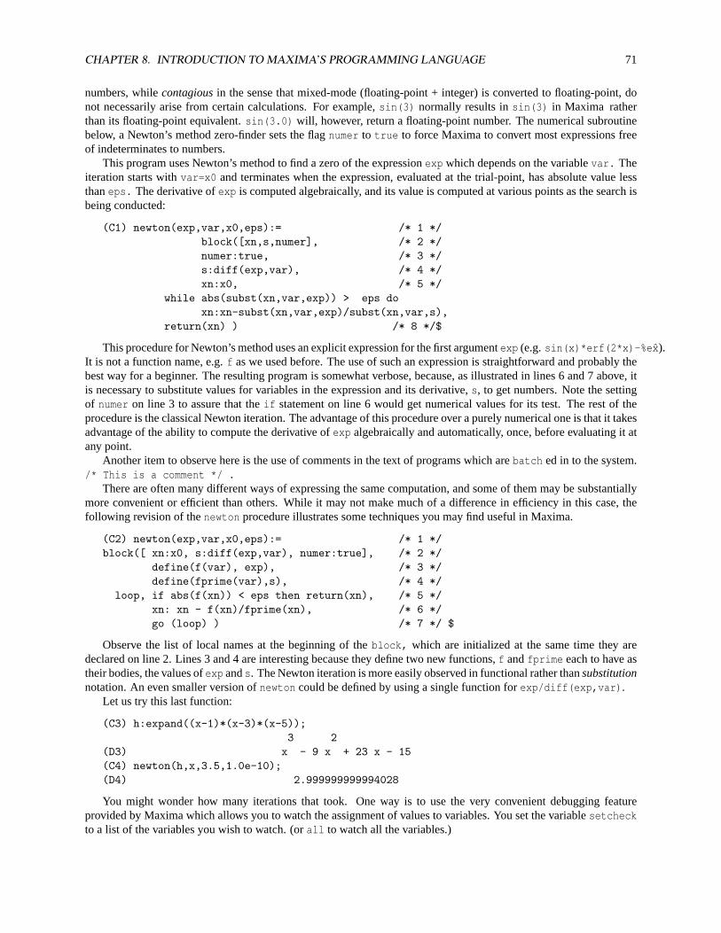
CHAPTER 8. INTRODUCTION TO MAXIMA’S PROGRAMMING LANGUAGE 71
numbers, whilecontagiousin the sense that mixed-mode (floating-point + integer) is converted to floating-point, donot necessarily arise from certain calculations. For example,sin(3) normally results insin(3) in Maxima ratherthan its floating-point equivalent.sin(3.0) will, however, return a floating-point number. The numerical subroutinebelow, a Newton’s method zero-finder sets the flagnumer to true to force Maxima to convert most expressions freeof indeterminates to numbers.
This program uses Newton’s method to find a zero of the expressionexp which depends on the variablevar. Theiteration starts withvar=x0 and terminates when the expression, evaluated at the trial-point, has absolute value lessthaneps. The derivative ofexp is computed algebraically, and its value is computed at various points as the search isbeing conducted:
(C1) newton(exp,var,x0,eps):= /* 1 */block([xn,s,numer], /* 2 */numer:true, /* 3 */s:diff(exp,var), /* 4 */xn:x0, /* 5 */
while abs(subst(xn,var,exp)) > eps doxn:xn-subst(xn,var,exp)/subst(xn,var,s),
return(xn) ) /* 8 */$
This procedure for Newton’s method uses an explicit expression for the first argumentexp (e.g.sin(x)*erf(2*x)-%ex̂).It is not a function name, e.g.f as we used before. The use of such an expression is straightforward and probably thebest way for a beginner. The resulting program is somewhat verbose, because, as illustrated in lines 6 and 7 above, itis necessary to substitute values for variables in the expression and its derivative,s, to get numbers. Note the settingof numer on line 3 to assure that theif statement on line 6 would get numerical values for its test. The rest of theprocedure is the classical Newton iteration. The advantage of this procedure over a purely numerical one is that it takesadvantage of the ability to compute the derivative ofexp algebraically and automatically, once, before evaluating it atany point.
Another item to observe here is the use of comments in the text of programs which arebatch ed in to the system./* This is a comment */ .
There are often many different ways of expressing the same computation, and some of them may be substantiallymore convenient or efficient than others. While it may not make much of a difference in efficiency in this case, thefollowing revision of thenewton procedure illustrates some techniques you may find useful in Maxima.
(C2) newton(exp,var,x0,eps):= /* 1 */block([ xn:x0, s:diff(exp,var), numer:true], /* 2 */
define(f(var), exp), /* 3 */define(fprime(var),s), /* 4 */
loop, if abs(f(xn)) < eps then return(xn), /* 5 */xn: xn - f(xn)/fprime(xn), /* 6 */go (loop) ) /* 7 */ $
Observe the list of local names at the beginning of theblock, which are initialized at the same time they aredeclared on line 2. Lines 3 and 4 are interesting because they define two new functions,f andfprime each to have astheir bodies, the values ofexp ands. The Newton iteration is more easily observed in functional rather thansubstitutionnotation. An even smaller version ofnewton could be defined by using a single function forexp/diff(exp,var).
Let us try this last function:
(C3) h:expand((x-1)*(x-3)*(x-5));3 2
(D3) x - 9 x + 23 x - 15(C4) newton(h,x,3.5,1.0e-10);(D4) 2.999999999994028
You might wonder how many iterations that took. One way is to use the very convenient debugging featureprovided by Maxima which allows you to watch the assignment of values to variables. You set the variablesetcheckto a list of the variables you wish to watch. (orall to watch all the variables.)
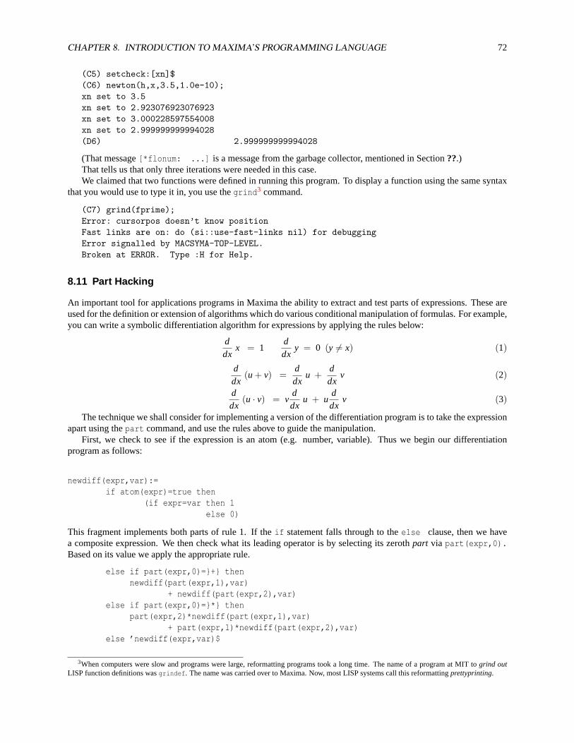
CHAPTER 8. INTRODUCTION TO MAXIMA’S PROGRAMMING LANGUAGE 72
(C5) setcheck:[xn]$(C6) newton(h,x,3.5,1.0e-10);xn set to 3.5xn set to 2.923076923076923xn set to 3.000228597554008xn set to 2.999999999994028(D6) 2.999999999994028
(That message[*flonum: ...] is a message from the garbage collector, mentioned in Section??.)That tells us that only three iterations were needed in this case.We claimed that two functions were defined in running this program. To display a function using the same syntax
that you would use to type it in, you use thegrind3 command.
(C7) grind(fprime);Error: cursorpos doesn’t know positionFast links are on: do (si::use-fast-links nil) for debuggingError signalled by MACSYMA-TOP-LEVEL.Broken at ERROR. Type :H for Help.
8.11 Part Hacking
An important tool for applications programs in Maxima the ability to extract and test parts of expressions. These areused for the definition or extension of algorithms which do various conditional manipulation of formulas. For example,you can write a symbolic differentiation algorithm for expressions by applying the rules below:
ddx
x = 1ddx
y = 0 (y 6= x) (1)
ddx
(u + v) =ddx
u +ddx
v (2)
ddx
(u · v) = vddx
u + uddx
v (3)
The technique we shall consider for implementing a version of the differentiation program is to take the expressionapart using thepart command, and use the rules above to guide the manipulation.
First, we check to see if the expression is an atom (e.g. number, variable). Thus we begin our differentiationprogram as follows:
newdiff(expr,var):=if atom(expr)=true then
(if expr=var then 1else 0)
This fragment implements both parts of rule 1. If theif statement falls through to theelse clause, then we havea composite expression. We then check what its leading operator is by selecting its zerothpart via part(expr,0).Based on its value we apply the appropriate rule.
else if part(expr,0)=}+} thennewdiff(part(expr,1),var)
+ newdiff(part(expr,2),var)else if part(expr,0)=}*} then
part(expr,2)*newdiff(part(expr,1),var)+ part(expr,1)*newdiff(part(expr,2),var)
else ’newdiff(expr,var)$
3When computers were slow and programs were large, reformatting programs took a long time. The name of a program at MIT togrind outLISP function definitions wasgrindef. The name was carried over to Maxima. Now, most LISP systems call this reformattingprettyprinting.
CHAPTER 8. INTRODUCTION TO MAXIMA’S PROGRAMMING LANGUAGE 73
Note the last clause which returns a ’newdiff form, that is, quoted, as a result when the program doesn’t know howto handle the leading operator. With some thought, you should now be able to extend newdiff to accommodateexpressions includingsin andcos as well as sums and products with more than two terms. (The Maxima languagedoes not at the moment have acase statement, which would make this particular program look better.) Is this stiil true
????
8.12 User Representation of Data
There is norecord or structuredata-typeconstructorin Maxima but there is a way of doing something similar. Ifyou have used a language like Pascal which has such a feature, you may appreciate its usefulness. Modern dialectsof LISP use such structures, but when Maxima was first designed and initially implemented (in 1967), this was not inwidespread use. It also influenced the user-level programming language.
It is natural to have to deal with collections of information in writing programs. For example, you might wish toprovide as input or output data, a pair of expressions representing a lower and an upper bound on a formula. One wayof handling this is by making up a newfunctionname, saybounds and using it as though it were a record designatoror constructor, but never associating it with an algorithm. Thusbounds(1,x) could be an expression representing theordered pair< 1,x >. Another example would be the use ofinteger_vector(1,3,5,7) to designate a sequence(presumably of arbitrary length, in general), of integers. There is a built-in form in Maxima namely alist, which can beused to deal with such collections. It is part of the LISP heritage indicated earlier that there was initially only one typeof structure: lists of any length or element type in Maxima. A list, when printed, looks like square-brackets enclosinga sequence of items. Thus you could express the bounds above as [1,x ]. However, if you used lists for all collections,you would not know, on the face of it, whether [1,2] was an instance ofbounds or integer_vector. Maximaallows you to designate functions you intend to treat as lists, although you can use a differentheaderlike boundswith each different type. Maxima makes available certain built-in functions which can then be used on such list-likeconstructions such asinteger_vector. These are declared by, for example,declare(integer_vector,list).The built-in operations includecons, append, member, endcons, map, rest.list2:cons(element,list1) returns a (new)list2 which has the given element inserted at the beginning oflist1; List1 andlist2 have a commonsharedtail.list3:append(list1,list2) returns a (new)list3 which is a combination of the two lists, sharing a common tailwith list2. Member(element,list) returns true or false depending on a test for membership.Endcons(element,list) returns an (unshared) list where the given element has been attached to the end of given listMap(fn,list) returns a new list where each element has had the function fn applied to it in turn.Rest(list,n) returns the part of the list beginning n items from the front.
These functions are parts of the fundamental repertoire of the programming language LISP.The use of list-like objects should be considered whenever you are dealing with a collection of elements: a set of
coordinates, a series of coefficients, a system of equations, a set of solutions, etc.Independent of thewhole listoperations above, Maxima has some selection and alteration operations which are
available on the same collections of data by the use of a numeric index. If you wish to use these indexing facilities,as we will illustrate for the notion ofcomplex below, youdeclare(complex,list). Then, if you define a complexnumber byx:complex(3,4) meaning thatx has real part 3, and imaginary part 4, the notationx[1]:10; is supported,and changes the value ofx to complex(10,4). The declaration explains to the Maxima system that the data structurefor complex will be implemented (in effect) as a list of items, and should be decomposable using the semantics of theMaxima list-handling commands. In fact, both selection and alteration is supported, and if you set the notation up by(real:1,imag:2)$ you can use the following command:x[imag]:-x[imag] to changex to its complex conjugate.
An important caution must be observed. When Maxima deals with compound structures, they are usually notrecopied, and if there are two names for the same object and the object is changed, then both names refer to the changedobject. If x andy refer to the samecomplex number, then changes tox[real] are also made to the correspondingcomponent ofy. If these items are to be kept separate,x:copylist(y); will give x a different representation, butwhose value is the same asy ’s. You can then change their components separately.
Maxima’s built-in lists mentioned earlier, which use square-brackets, can be altered and selected by indexing.There are two other compound structures in Maxima which we mention here, which may be useful for collections
of data: arrays and matrices. The matrix form is useful for two-dimensional rectangular tables of data. The matrixdata format is supported by a number of special commands oriented toward the conventional interpretation of matricesin mathematics: inverses, determinants, etc. Matrices can be used for other kinds of data, but you should be cautious
CHAPTER 8. INTRODUCTION TO MAXIMA’S PROGRAMMING LANGUAGE 74
about using them in a manner that is too far distant from the conventional: arithmetic operations in Maxima inparticular, have already been defined.
Arrays are unusual in their flexibility in Maxima. They are usually treated as global tables, although they can bedeclared to be local to a function; they cannot be passed around as parameters as is the case with matrices. The namesof arrays may be passed from program to program, but the data itself is not recopied, nor is it convenient to evenmake a copy of the data into another array.Hashedarrays are particularly ingenious, and have been illustrated earlier.Functions can be associated with arrays to provide new values for entries as they are required.
At this point you should be able to make use of the Maxima manual to learn more details for representation of newdata types as you develop your application.
The true programming buff may also be interested in the macro-expansion capabilities of Maxima and its extensiblesyntax. At this point we would discourage the use of these facilities by novices, but encourage their use by personswilling to experiment in providing the most versatile user-oriented packages within the Maxima framework.
There is acompilationfacility which allows users to translate Maxima code into potentially faster running code.Since most of the time in most programs is used by calls to LISP programs, this is usually ineffective. In general, thisshould be avoided by novices and most experienced users, since time spent on this is more wisely spent on mathemati-cal restructuring of the solution method, or (in the case of primarily numerical computation), using a numerical libraryroutine written in a suitable language.
CHAPTER 9
Graphics and Forms of Output
In addition to some options with respect to the mathematical output from Maxima on the command line, the systemis also capable of interfacing with external programs to provide graphing capabilities. You can also save Maximasessions to reload later.
9.1 Options on the Command Line
While for normal use the default settings are likely to be preferable, Maxima allows you to set some options withregards to how output is returned.
9.1.1. 1D vs. 2D
The default output Maxima gives you when you evaluate an expression is 2D output, which basically means you havesome visual feedback on the structure of things like fractions and integrals as ascii art, and the output expression is notone string. Normally this is a good thing, but if for any reason you wish to turn that feature off, it is quite possible to doso. Maxima has an internal variable regulating this feature calledDISPLAY2D. Ordinarily it is set to TRUE, providingthe typical ascii Maxima output you would get in a terminal session. Setting it to FALSE will cause returns to be asingle string. Here is an example:
(C1) 2*y*3*x/(4*x+y+3/4);6 x y
(D1) -----------3
y + 4 x + -4
(C2) DISPLAY2D:FALSE;(D2) FALSE(C3) 2*y*3*x/(4*x+y+3/4);(D3) 6*x*y/(y+4*x+3/4)
One important note here is that if you only wish to change the dimension of your output for one entry, you mustset this variable by hand both before and after the command - i.e.,ev(2/3,DISPLAY2D:FALSE) will not result in2/3unless the DISPLAY2D:FALSE command has already been entered - ev will not use it in its evaluation.
9.1.2. TeX Strings as Output
As you probably already know, Maxima is able to output expressions in TeX format. This ability is used transparentlyin several places, but you can also request this output manually, using thetex(expression) command.
75
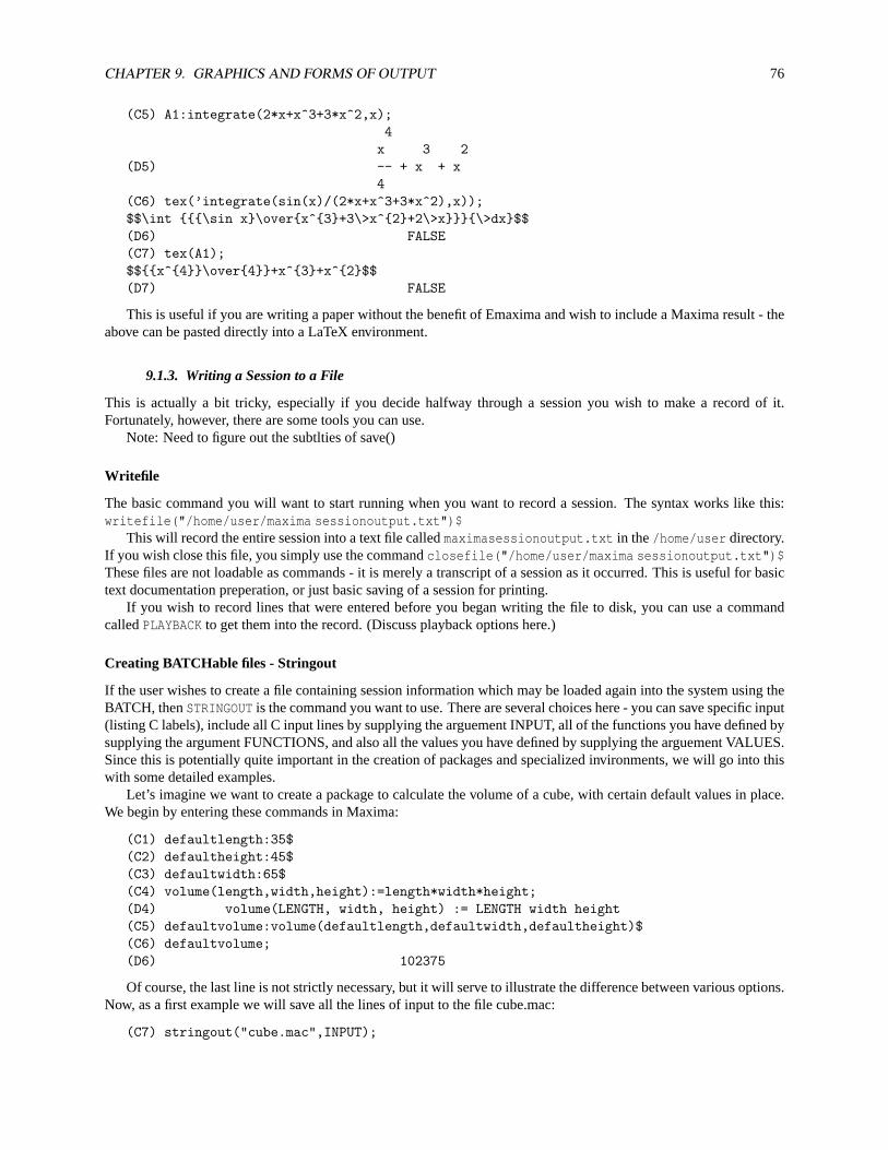
CHAPTER 9. GRAPHICS AND FORMS OF OUTPUT 76
(C5) A1:integrate(2*x+x^3+3*x^2,x);4
x 3 2(D5) -- + x + x
4(C6) tex(’integrate(sin(x)/(2*x+x^3+3*x^2),x));$$\int {{{\sin x}\over{x^{3}+3\>x^{2}+2\>x}}}{\>dx}$$(D6) FALSE(C7) tex(A1);$${{x^{4}}\over{4}}+x^{3}+x^{2}$$(D7) FALSE
This is useful if you are writing a paper without the benefit of Emaxima and wish to include a Maxima result - theabove can be pasted directly into a LaTeX environment.
9.1.3. Writing a Session to a File
This is actually a bit tricky, especially if you decide halfway through a session you wish to make a record of it.Fortunately, however, there are some tools you can use.
Note: Need to figure out the subtlties of save()
Writefile
The basic command you will want to start running when you want to record a session. The syntax works like this:writefile("/home/user/maxima sessionoutput.txt")$
This will record the entire session into a text file calledmaximasessionoutput.txt in the/home/user directory.If you wish close this file, you simply use the commandclosefile("/home/user/maxima sessionoutput.txt")$These files are not loadable as commands - it is merely a transcript of a session as it occurred. This is useful for basictext documentation preperation, or just basic saving of a session for printing.
If you wish to record lines that were entered before you began writing the file to disk, you can use a commandcalledPLAYBACK to get them into the record. (Discuss playback options here.)
Creating BATCHable files - Stringout
If the user wishes to create a file containing session information which may be loaded again into the system using theBATCH, thenSTRINGOUT is the command you want to use. There are several choices here - you can save specific input(listing C labels), include all C input lines by supplying the arguement INPUT, all of the functions you have defined bysupplying the argument FUNCTIONS, and also all the values you have defined by supplying the arguement VALUES.Since this is potentially quite important in the creation of packages and specialized invironments, we will go into thiswith some detailed examples.
Let’s imagine we want to create a package to calculate the volume of a cube, with certain default values in place.We begin by entering these commands in Maxima:
(C1) defaultlength:35$(C2) defaultheight:45$(C3) defaultwidth:65$(C4) volume(length,width,height):=length*width*height;(D4) volume(LENGTH, width, height) := LENGTH width height(C5) defaultvolume:volume(defaultlength,defaultwidth,defaultheight)$(C6) defaultvolume;(D6) 102375
Of course, the last line is not strictly necessary, but it will serve to illustrate the difference between various options.Now, as a first example we will save all the lines of input to the file cube.mac:
(C7) stringout("cube.mac",INPUT);
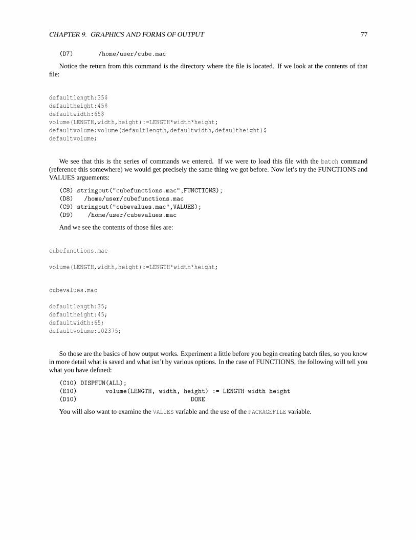
CHAPTER 9. GRAPHICS AND FORMS OF OUTPUT 77
(D7) /home/user/cube.mac
Notice the return from this command is the directory where the file is located. If we look at the contents of thatfile:
defaultlength:35$defaultheight:45$defaultwidth:65$volume(LENGTH,width,height):=LENGTH*width*height;defaultvolume:volume(defaultlength,defaultwidth,defaultheight)$defaultvolume;
We see that this is the series of commands we entered. If we were to load this file with thebatch command(reference this somewhere) we would get precisely the same thing we got before. Now let’s try the FUNCTIONS andVALUES arguements:
(C8) stringout("cubefunctions.mac",FUNCTIONS);(D8) /home/user/cubefunctions.mac(C9) stringout("cubevalues.mac",VALUES);(D9) /home/user/cubevalues.mac
And we see the contents of those files are:
cubefunctions.mac
volume(LENGTH,width,height):=LENGTH*width*height;
cubevalues.mac
defaultlength:35;defaultheight:45;defaultwidth:65;defaultvolume:102375;
So those are the basics of how output works. Experiment a little before you begin creating batch files, so you knowin more detail what is saved and what isn’t by various options. In the case of FUNCTIONS, the following will tell youwhat you have defined:
(C10) DISPFUN(ALL);(E10) volume(LENGTH, width, height) := LENGTH width height(D10) DONE
You will also want to examine theVALUES variable and the use of thePACKAGEFILE variable.
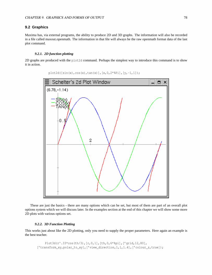
CHAPTER 9. GRAPHICS AND FORMS OF OUTPUT 78
9.2 Graphics
Maxima has, via external programs, the ability to produce 2D and 3D graphs. The information will also be recordedin a file called maxout.openmath. The information in that file will always be the raw openmath format data of the lastplot command.
9.2.1. 2D function plotting
2D graphs are produced with theplot2d command. Perhaps the simplest way to introduce this command is to showit in action.
plot2d([sin(x),cos(x),tan(x)],[x,0,2*%Pi],[y,-1,1]);
These are just the basics - there are many options which can be set, but most of them are part of an overall plotoptions system which we will discuss later. In the examples section at the end of this chapter we will show some more2D plots with various options set.
9.2.2. 3D Function Plotting
This works just about like the 2D plotting, only you need to supply the proper parameters. Here again an example isthe best teacher.
Plot3d(r^.33*cos(th/3),[r,0,1],[th,0,6*%pi],[’grid,12,80],[’transform_xy,polar_to_xy],[’view_direction,1,1,1.4],[’colour_z,true]);
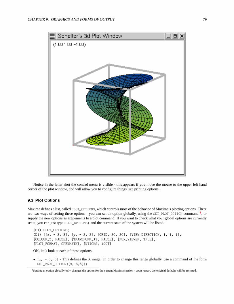
CHAPTER 9. GRAPHICS AND FORMS OF OUTPUT 79
Notice in the latter shot the control menu is visible - this appears if you move the mouse to the upper left handcorner of the plot window, and will allow you to configure things like printing options.
9.3 Plot Options
Maxima defines a list, calledPLOT_OPTIONS, which controls most of the behavior of Maxima’s plotting options. Thereare two ways of setting these options - you can set an option globally, using theSET_PLOT_OPTION command1, orsupply the new options as arguements to a plot command. If you want to check what your global options are currentlyset at, you can just typePLOT_OPTIONS; and the current state of the system will be listed.
(C1) PLOT_OPTIONS;(D1) [[x, - 3, 3], [y, - 3, 3], [GRID, 30, 30], [VIEW_DIRECTION, 1, 1, 1],[COLOUR_Z, FALSE], [TRANSFORM_XY, FALSE], [RUN_VIEWER, TRUE],[PLOT_FORMAT, OPENMATH], [NTICKS, 100]]
OK, let’s look at each of these options.
• [x, - 3, 3] - This defines the X range. In order to change this range globally, use a command of the formSET_PLOT_OPTION([x,-5,5]);
1Setting an option globally only changes the option for the current Maxima session - upon restart, the original defaults will be restored.
CHAPTER 9. GRAPHICS AND FORMS OF OUTPUT 80
• [y, - 3, 3] - This defines the Y range. In order to change this range globally, use a command of the formSET_PLOT_OPTION([y,-5,5]);
• [GRID, 30, 30] - This controls, in 3D plotting, the number of points used to draw the figure. The functionis only calculated at a certain number of points - after that, linear approximations are drawn. Globally, usee acommand of the formSET_PLOT_OPTION([GRID,40,35]);
• [VIEW_DIRECTION, 1, 1, 1] - This option is specific to the case when the plot command outputs directly topostscript in 3D(SeePLOT_FORMAT.) It determines the direction from which the ’camera’ looks at the function,which is along a line parallel to the line fromVIEW_DIRECTION to the origin. It only needs to be set in the caseof postscript output; it is ignored otherwise. Globally, use a command of the formSET_PLOT_OPTION([VIEW_DIRECTION,1.4,1.4,1.4]);
• [COLOUR_Z, FALSE] - This refers also to the postscript output - if set to TRUE it provides a little color shadingin the output. Form isSET_PLOT_OPTION([COLOUR_Z, TRUE]);
• [TRANSFORM_XY, FALSE] - This appears to provide the ability to produce plots with different coordinate sys-tems, but I am unsure of how to make it work. Need to get help here.
• [RUN_VIEWER, TRUE] - If you only wish Maxima to output the openmath file and not launch the graphicalviewer, set this option to false. Remember, however, that if you wish to run multiple commands to generatedata you will have to recover the information from the maxout.openmath file each time, because each new plotcommand will overwrite it. Form isSET_PLOT_OPTION([RUN_VIEWER, FALSE]);
• [NTICKS, 100] - Controls the number of points used to draw the 2D plots - the program will calculate the valueof the function at N points, and then draw lines between them. Form isSET_PLOT_OPTION([NTICKS, 200]);
• [PLOT_FORMAT, OPENMATH] - This controls which program gets the output from Maxima for display. Thereare currently four viable options - OPENMATH, GNUPLOT, GEOMVIEW, and PS. PS is simply direct outputto a postscript file, maxout.ps. All of these programs are freely available. Geomview is currently Unix only,and is available at http://geomview.sourceforge.net as both source and binary. Openmath is distributed as partof Maxima. Gnuplot is widely available, with a homepage at http://www.gnuplot.org and the most currentdevelopment version at http://sourceforge.net/projects/gnuplot. Gnuplot can run on both Windows and Linux.
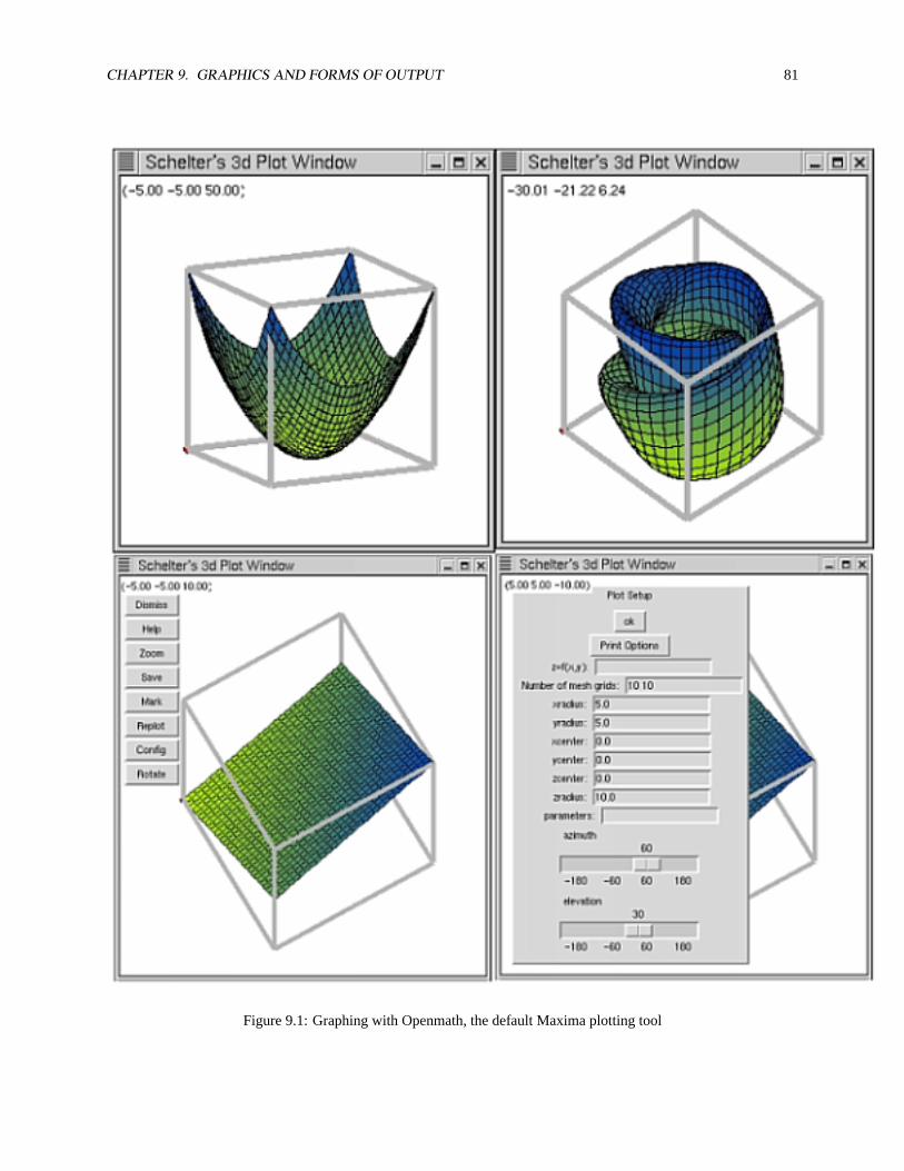
CHAPTER 9. GRAPHICS AND FORMS OF OUTPUT 81
Figure 9.1: Graphing with Openmath, the default Maxima plotting tool

CHAPTER 9. GRAPHICS AND FORMS OF OUTPUT 82
Figure 9.2: Graphing with gnuplot, using the mgnuplot utility
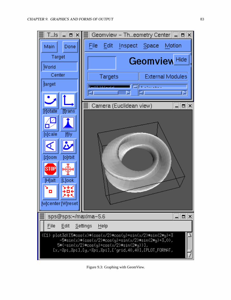
CHAPTER 9. GRAPHICS AND FORMS OF OUTPUT 83
Figure 9.3: Graphing with GeomView.
CHAPTER 10
Maxims for the Maxima User
Some beginning users of algebraic manipulation systems find that their previous experiences with traditional program-ming systems do not translate easily into algebraic programming; others find Maxima descriptions inadequate becausethe emphasis is on the mixture of mathematical notations and algorithms, and not onefficientuse of machine or humanresources (no one likes to wait longer than necessary for an answer!). While we cannot provide a complete educationin efficient and effective programming, we have collected a fewmaximsin an attempt to help you with some of thesestart-upproblems.
Algebraic manipulation is a new and different computational approach for which prior experience withcomputational methods may be misleading. You should attempt to learn the ways in which algebraicmanipulation differs from other approaches.
For example, consider the problem of inverting ann×n matrix. In numerical analysis we learn that the problemrequires on the order ofn3 operations. Theoreticians will point out that forn sufficiently large, one can reduce thenumber of multiplications belown3 to n2.8. This analysis is unfortunately not relevant in dealing with matrices withsymbolic entries. Consider the number of terms in the determinant of the generaln×n matrix whose elements arethe symbolsai, j . When the inverse is written out in a fully expanded form, just the determinant (a necessary part ofrepresenting the inverse) hasn! terms. It is impossible to compute this determinant in less thantime proportional to n!In fact, for largen, it is just not feasible to compute this form explicitly on existing computers. The combinatorial orexponential character that some algebraic manipulation problems have when they are approached with an inefficientalgorithm, makes for a vastly different game from, say, numerical computation, where the size of objects is generallyknown at the onset of the calculation, and does not increase.
Needlessly generalizing a problem usually results in unnecessary expense.
For example, if you wish to obtain determinants for a collection of matrices whose general pattern of entries is rep-resented by parametric formulas, you might consider obtaining the determinant of the general matrix and substitutingvarious values for the parameters into the result. This may work for matrices of low order, but is probably a poor planfor dealing with the exponential growth inherent in computing symbolic determinants. It would probably be better tosubstitute the parameters first, since this would drastically reduce the cost of the determinant calculation.
Sometimes, when humans are dealing with formulas, it is preferable to use an indeterminate, sayG in a formulawhich is really known to be, say, 3/5. On the other hand, it is likely (although not certain!) that the calculation using3/5 will take less time than the calculation withG. Since the cost inherent in some computations is usually a function ofthe number of variables in the expression,it pays to reduce the number of variables in a problem as much as possible.
You should be aware of the types of calculations which in the general case have exponential growth(e.g.many matrix calculations with symbolic entries, repeated differentiation of products or quotients, solutionof systems of polynomial equations).
Your should anticipate a certain amount of trial-and-error in calculations.
84
CHAPTER 10. MAXIMS FOR THE MAXIMA USER 85
Just as in other problem-solving activities, often the first technique that comes to mind is not the best. While itoccasionally happens that brute force carries the day, cleverness in computing can be as important as cleverness in handcalculations. It is natural, during hand calculations, to apply critical simplificiations or substitutions in computations.These simplifications include collecting terms selectively or striking out terms which do not ultimately contributeto the final answer because of physical interpretations. Computer algorithms which do not incorporate these sametricks may bog down surprisingly soon. Thinking about these shortcuts may be important. In fact, it is one of themore rewarding aspects of computer algebra systems that they give the problem solver an opportunity to organize,encapsulate and distribute a particularly clever piece of mathematical manipulation.
Try to reduce your problem so that it can be performed in a simpler domain.
For example, if your problem appears to involve trigonometric functions, logs, exponentials, etc. see if you can reduceit to a rational function (ratio of polynomials) problem. If it appears to be a rational function, see if you can, bysubstitutions, make it into a polynomial problem, or a truncated power-series problem. If it appears to be a probleminvolving rational numbers, consider the use of floating-point numbers as an alternative, if the growth in the size ofnumbers presents difficulties.
There are other special forms that are especially efficient. In a number of areas of investigationit pays to convertall expressions to the internal rational form (usingrat) or into Poisson-series form (usingintopois) to avoid theoverhead the the general representation. The price you may pay here is thtat the structure of the formulas maybe significantly different from those you began with: The canonical transformations used by these representationsdrastically re-order, expand, and modify the original expressions.
Sometimes someone else has already started on your problem.
You should look through thesharedirectory programs available to see if there are contributed packages that mightbe of use either as subroutines or as models for programming. You should also consider writing programs that youdevelop in solving your problems in a form suitable for sharing with others.
Pattern matching allows you to tune the system simplifier to your application, and develop rule-replacementprograms.
Learning to use the pattern-matching facilities effectively is a nontrivial task. Nevertheless if you have a fairlycomplex problem involvilng the recognition and application of identities, you should consider making an effort to usethese facilities. In recent years, advocates ofrule-based expert systemshave claimed that this type of formalism can orshould be used to incorporate varied types of knowledge. Algebraic manipulation programs have depended on patternmatching since at least 1961, for some of their power.
Finally, we would like to point out that algebraic manipulation systems, in spite of their pitfalls, can be of majorassistance in solving difficult problems. If you are willing to invest some time in learning, there may be enormousbenefits in using such a system. We think it is unfortunate that some users reserve Maxima for difficult problems.Those of us who have grown up with Maxima near at hand find it of great use in routine computations as well.
CHAPTER 11
Help Systems and Debugging
Using the debugger and the online help system.
86
CHAPTER 12
Troubleshooting
Common errors, their cause and solution.
87
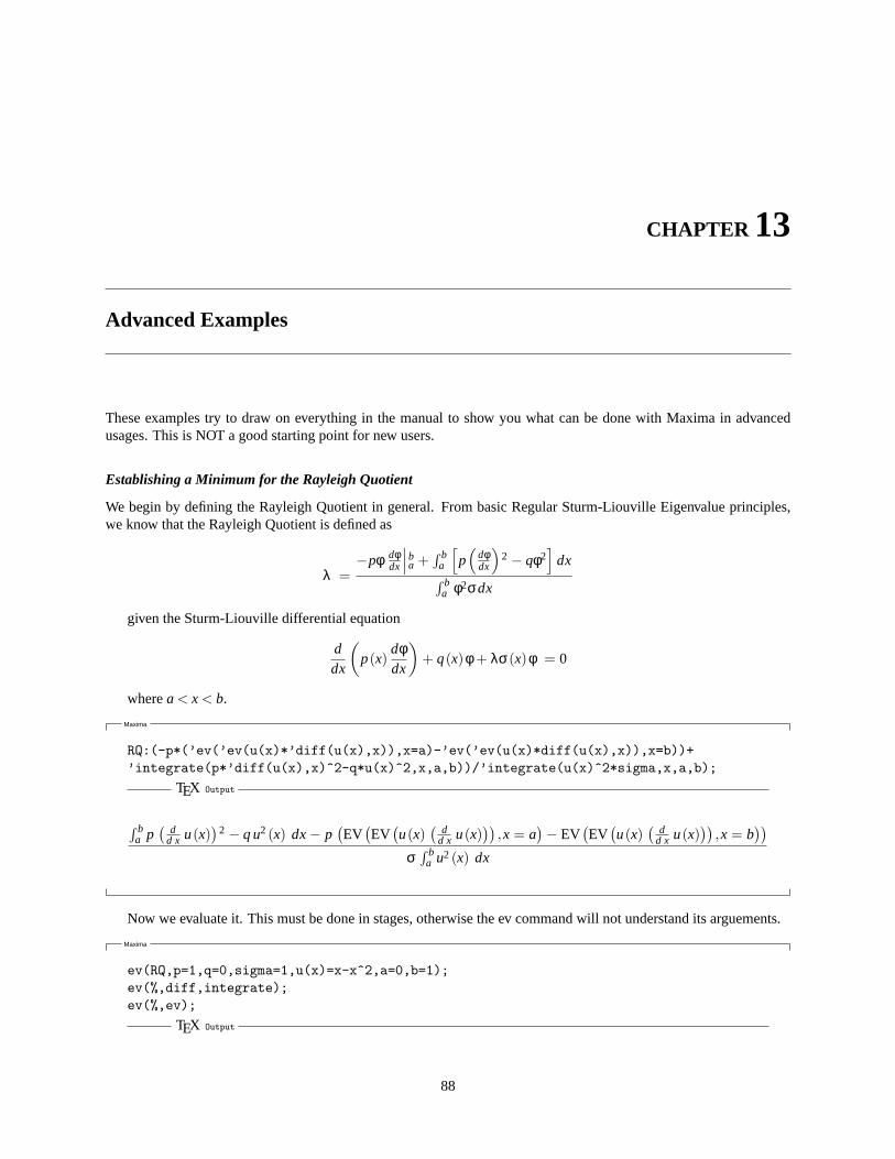
CHAPTER 13
Advanced Examples
These examples try to draw on everything in the manual to show you what can be done with Maxima in advancedusages. This is NOT a good starting point for new users.
Establishing a Minimum for the Rayleigh Quotient
We begin by defining the Rayleigh Quotient in general. From basic Regular Sturm-Liouville Eigenvalue principles,we know that the Rayleigh Quotient is defined as
λ =−pφ dφ
dx
∣∣∣ba +R b
a
[p(
dφdx
)2 − qφ2
]dxR b
a φ2σdx
given the Sturm-Liouville differential equation
ddx
(p(x)
dφdx
)+ q(x)φ + λσ(x)φ = 0
wherea < x < b.
Maxima
RQ:(-p*(’ev(’ev(u(x)*’diff(u(x),x)),x=a)-’ev(’ev(u(x)*diff(u(x),x)),x=b))+’integrate(p*’diff(u(x),x)^2-q*u(x)^2,x,a,b))/’integrate(u(x)^2*sigma,x,a,b);
TEX Output
R ba p(
dd x u(x)
)2 − q u2 (x) dx− p
(EV(EV(u(x)
(d
d x u(x)))
,x = a)− EV
(EV(u(x)
(d
d x u(x)))
,x = b))
σR b
a u2 (x) dx
Now we evaluate it. This must be done in stages, otherwise the ev command will not understand its arguements.
Maxima
ev(RQ,p=1,q=0,sigma=1,u(x)=x-x^2,a=0,b=1);ev(%,diff,integrate);ev(%,ev);
TEX Output
88
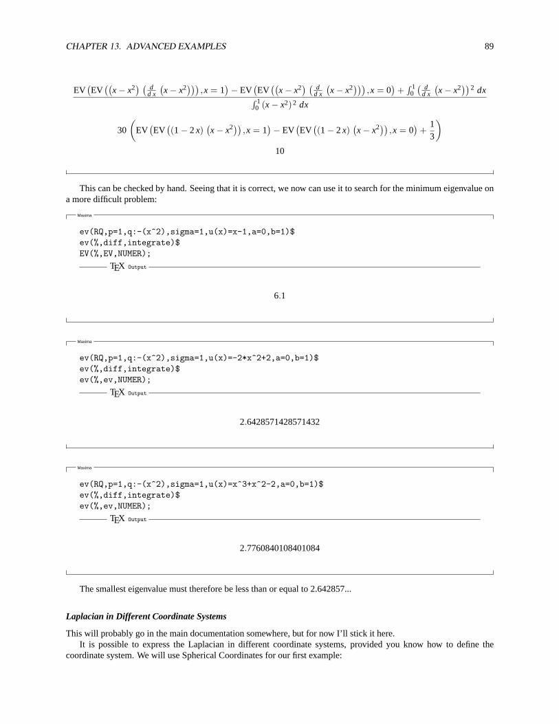
CHAPTER 13. ADVANCED EXAMPLES 89
EV(EV((
x− x2) (
dd x
(x− x2
))),x = 1
)− EV
(EV((
x− x2) (
dd x
(x− x2
))),x = 0
)+
R 10
(d
d x
(x− x2
))2 dxR 1
0 (x− x2)2 dx
30
(EV(EV((1− 2x)
(x− x2)) ,x = 1
)− EV
(EV((1− 2x)
(x− x2)) ,x = 0
)+
13
)10
This can be checked by hand. Seeing that it is correct, we now can use it to search for the minimum eigenvalue ona more difficult problem:
Maxima
ev(RQ,p=1,q:-(x^2),sigma=1,u(x)=x-1,a=0,b=1)$ev(%,diff,integrate)$EV(%,EV,NUMER);
TEX Output
6.1
Maxima
ev(RQ,p=1,q:-(x^2),sigma=1,u(x)=-2*x^2+2,a=0,b=1)$ev(%,diff,integrate)$ev(%,ev,NUMER);
TEX Output
2.6428571428571432
Maxima
ev(RQ,p=1,q:-(x^2),sigma=1,u(x)=x^3+x^2-2,a=0,b=1)$ev(%,diff,integrate)$ev(%,ev,NUMER);
TEX Output
2.7760840108401084
The smallest eigenvalue must therefore be less than or equal to 2.642857...
Laplacian in Different Coordinate Systems
This will probably go in the main documentation somewhere, but for now I’ll stick it here.It is possible to express the Laplacian in different coordinate systems, provided you know how to define the
coordinate system. We will use Spherical Coordinates for our first example:
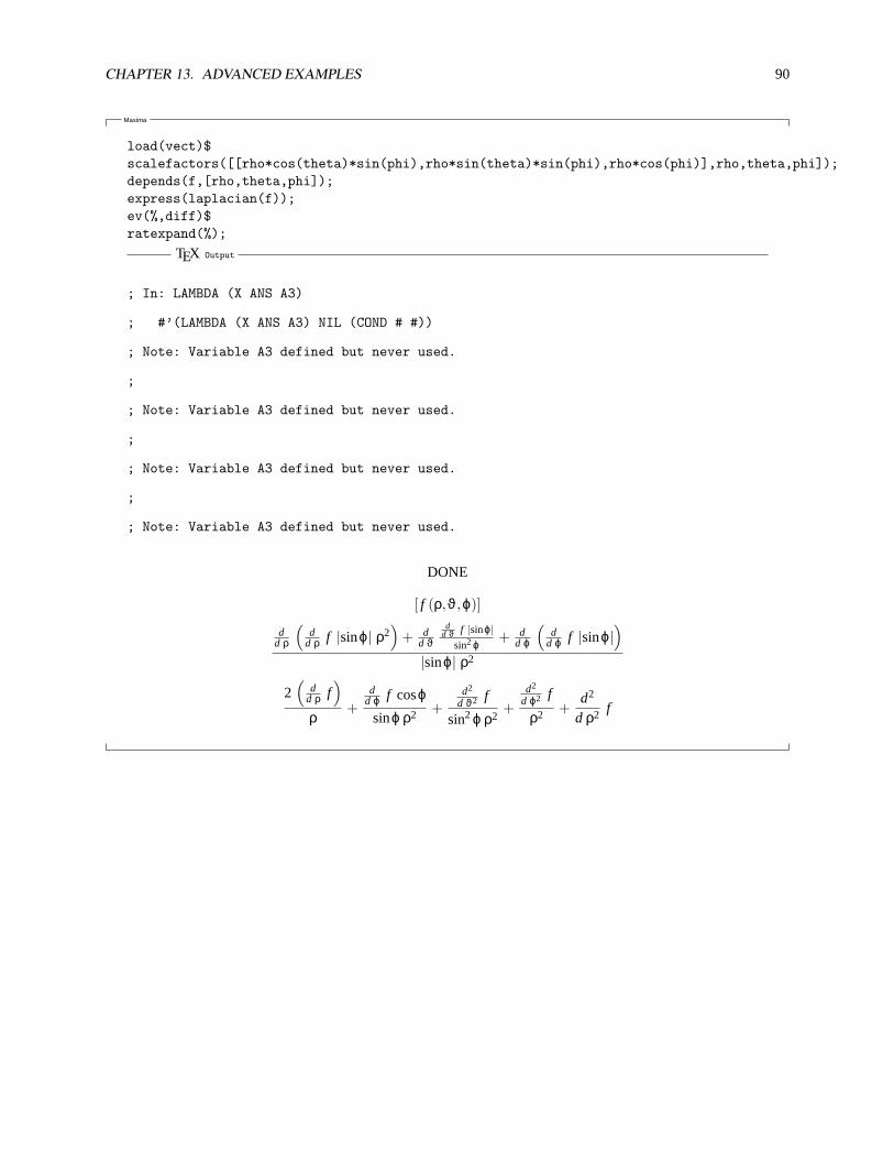
CHAPTER 13. ADVANCED EXAMPLES 90
Maxima
load(vect)$scalefactors([[rho*cos(theta)*sin(phi),rho*sin(theta)*sin(phi),rho*cos(phi)],rho,theta,phi]);depends(f,[rho,theta,phi]);express(laplacian(f));ev(%,diff)$ratexpand(%);
TEX Output
; In: LAMBDA (X ANS A3)
; #’(LAMBDA (X ANS A3) NIL (COND # #))
; Note: Variable A3 defined but never used.
;
; Note: Variable A3 defined but never used.
;
; Note: Variable A3 defined but never used.
;
; Note: Variable A3 defined but never used.
DONE
[ f (ρ,ϑ,ϕ)]
dd ρ
(d
d ρ f |sinϕ| ρ2)
+ dd ϑ
dd ϑ f |sinϕ|
sin2 ϕ+ d
d ϕ
(d
d ϕ f |sinϕ|)
|sinϕ| ρ2
2(
dd ρ f
)ρ
+d
d ϕ f cosϕsinϕ ρ2 +
d2
d ϑ2 f
sin2 ϕ ρ2+
d2
d ϕ2 f
ρ2 +d2
d ρ2 f
Part II
External, Additional, and ContributedPackages
91
CHAPTER 14
The Concept of Packages - Expanding Maxima’s Abilities
This chapter will try to give some in depth information on the why and how of Maxima packages. It is true that many“standard” abilities of Maxima, such as vectors, are due to packages, but this part of the book will deal with morespecialized contributed packages, such as elliptical integrals, special scientific packages, etc. That way the first part ofthe book can be rewritten less frequently, but we can still have all the information here.
92
CHAPTER 15
Available Packages for Maxima
Maybe we can do this in one chapter, maybe each package will warrant a chapter. Not sure. For now, I’ll assume oneSection per package, not one Chapter.
93
List of Figures
3.1 Maxima-mode. . . . . . . . . . . . . . . . . . . . . . . . . . . . . . . . . . . . . . . . . . . . . . .163.2 Enhanced Terminal Mode. . . . . . . . . . . . . . . . . . . . . . . . . . . . . . . . . . . . . . . . .183.3 An Emaxima Session. . . . . . . . . . . . . . . . . . . . . . . . . . . . . . . . . . . . . . . . . . .193.4 TeXmacs with a Maxima Session. . . . . . . . . . . . . . . . . . . . . . . . . . . . . . . . . . . . . 33
9.1 Graphing with Openmath, the default Maxima plotting tool. . . . . . . . . . . . . . . . . . . . . . . 819.2 Graphing with gnuplot, using the mgnuplot utility. . . . . . . . . . . . . . . . . . . . . . . . . . . . 829.3 Graphing with GeomView.. . . . . . . . . . . . . . . . . . . . . . . . . . . . . . . . . . . . . . . .83
94
Index
CompilingCLISP, 9CMULISP, 10GCL, 8
DebuggingExiting, 33
Exiting, 33
Hiding output, 34
Quitting, 33
95
Bibliography
[AAC93] AACC, editor. Proceedings of the 1993 American Control Conference: The Westin St. Francis Hotel,San Francisco, California, June 2–4, 1993, 1109 Spring Street, Suite 300, Silver Spring, MD 20910,USA, 1993. IEEE Computer Society Press. Three volumes.15
[ABC+88] O. Akhrif, G. L. Blankenship, P. Chancelier, C. Gomez, J. P. Quadrat, and A. Sulem. Integration ofsymbolic and numerical processing in control engineering design. In IEEE, editor,Digest of Papers:Compcon Spring ’88. Thirty-Third IEEE Computer Society International Conference, 29 February –3 March 1988, Cathedral Hill Hotel, San Francisco, California, pages 482–485, 1109 Spring Street,Suite 300, Silver Spring, MD 20910, USA, 1988. IEEE Computer Society Press.
[ACM85] Proceedings of the ACM SIGPLAN 85 Symposium on Language Issues in Programming Environments:papers presented at the symposium in Seattle, Washington, 25–28 June, 1985, New York, NY, USA,1985. ACM Press. Published in ACM SIGPLAN notices, volume 20, number 7.15
[ACM89] ACM, editor. Proceedings of the ACM-SIGSAM 1989 International Symposium on Symbolic andAlgebraic Computation, ISSAC ’89, 17–19 July 1989, Portland, OR, USA, New York, NY, USA, 1989.ACM Press. 15
[AG87] George C. Atallah and James Geer. Non-linear oscillations with multiple forcing terms.InternationalJournal of Non-Linear Mechanics, 22(6):439–449, 1987.
[Akm88] Varol Akman. Geometry and graphics applied to robotics. In Earnshaw [Ear88], pages 619–638.
[AM89] H. Ashrafiuon and N. K. Mani. Applications of symbolic computing for numerical analysis of mechan-ical systems.American Society of Mechanical Engineers, Design Engineering Division (Publication)DE, 19-3(pt 3):141–149, 1989.
[AM90] H. Ashrafiuon and N. K. Mani. Analysis and optimal design of spatial mechanical systems.Journalof Mechanisms, Transmissions, and Automation in Design, 112(2):200–207, June 1990.
[And84] George E. Andrews. Ramanujan and SCRATCHPAD. In Golden and Hussain [GH84], pages 383–??
[ANGK+87] V. C. Aguilera-Navarro, R. Guardiola, C. Keller, M. de Llano, M. Popovic, and M. Fortes. Van derWaals perturbation theory for Fermion and Boson ground-state matter.Phys. Rev. A, 35(9):3901–3910,May 1987.
[Ano75] Anonymous.MACSYMA primer. Massachusetts Institute of Technology, Mathlab Group, Cambridge,MA, USA, 1975.
[Ano78] Anonymous.MACSYMA primer. Massachusetts Institute of Technology, Mathlab Group, Cambridge,MA, USA, revised edition, 1978.
[Ano80] Anonymous, editor.Conference record of the 1980 LISP Conference: papers presented at StanfordUniversity, Stanford, California, August 25–27, 1980, New York, NY, USA, 1980. ACM Press.15
[Ano84] Anon. 54th symposium on shock and vibration.Shock and Vibration Bulletin, June 1984.
96

BIBLIOGRAPHY 97
[Ano88] Anonymous.MACSYMA user’s guide. Symbolics, Inc., 11 Cambridge Center, Cambridge MA 02142,USA, 1988.
[Ano92] Anonymous.MACSYMA user’s guide. Macsyma, Inc., Arlington, MA, USA, 1992.
[Ano95a] Anonymous. Mathematik — komfortabel und preiswert: Macsyma 2.0 für Windows.Elektronik,44(5):154–??, 1995.
[Ano95b] Anonymous. Software forum.Design news, 50(8):134–??, April 1995.
[AP90] M. D. Abouzahra and R. Pavelle. Computer algebra applied to radiation from microstrip discontinu-ities. Journal of Symbolic Computation, 10(5):525–528, November 1990.
[Ari89] N. Ari. Application of computer code MACSYMA for electromagnetics. In Hamza [Ham89], pages77–80.
[Baj86] Chanderjit Bajaj. Proving geometric algorithm non-solvability: An application of factoring polynomi-als. Journal of Symbolic Computation, 2(1):99–102, March 1986.
[Ban84] Kenneth A. Bannister. MACSYMA-aided large deformation analysis of a cylindrical shell under purebending. In Golden and Hussain [GH84], pages 140–??
[Bar90] Jon Barwise. Computers and mathematics.Notices Amer. Math. Soc., 37(1):7–??, January 1990.
[Bau88] H. H. Bau. Symbolic computation — an introduction for the uninitiated.American Society of Me-chanical Engineers, Heat Transfer Division, (Publication) HTD, 105:1–10, 1988.
[BBR85] N. Bessis, G. Bessis, and D. Roux. Closed-form expressions for the Dirac-Coulomb radialrt integrals.Phys. Rev. A, 32:2044–2050, 1985.
[Ber84] Robert H. Berman. Measuring the performance of a computational physics environment. In Goldenand Hussain [GH84], pages 244–??
[Bey79] W. A. Beyer. Lie group theory for symbolic integration of first order ordinary differential equations.In Lewis [Lew79], pages 362–384.
[Bey84] William A. Beyer. Solution of simultaneous polynomial equations by elimination in MACSYMA. InGolden and Hussain [GH84], pages 110–??
[BFBZ92] Eva Bozoki, Aharon Friedman, and Ilan Ben-Zvi. ASAP — A symbolic algebra package for acceler-ator design. In IEEE [IEE92a], pages 272–274. Five volumes. IEEE catalog no. 91CH3038-7.
[BFHS92] W. A. Beyer, L. R. Fawcett, L. P. Harten, and B. K. Swartz. The volume common to two congruentcircular cylinders.Journal of Symbolic Computation, 13(2):221–230, February 1992.
[BFMS87] W. A. Beyer, L. R. Fawcett, R. D. Mauldin, and B. K. Swartz. The volume common to two congruentcircular cones whose axes intersect symmetrically.Journal of Symbolic Computation, 4(3):381–390,December 1987.
[BG83] Richard Bogen and Jeffrey Golden.MACSYMA reference manual. Massachusetts Institute of Tech-nology, Mathlab Group, Cambridge, MA, USA, version 10, first printing edition, 1983.
[BGGD77] Richard Bogen, Jeffrey Golden, Michael Genesereth, and Alexander Doohovskoy.MACSYMA refer-ence manual: version nine. Massachusetts Institute of Technology, Cambridge, MA, USA, 1977.
[BH87] W. A. Beyer and L. Heller. A Steiner tree associated with tree quarks.Journal of Symbolic Computa-tion, 3(3):283–289, June 1987.
[BHY88] Haim H. Bau, Thorwald Herbert, and M. M. Yovanovich, editors.Symbolic Computation in Fluid Me-chanics and Heat Transfer, volume 105 ofAmerican Society of Mechanical Engineers, Heat TransferDivision, (Publication) HTD, 345 E. 47th St., New York, NY 10017, USA, 1988. American Societyof Mechanical Engineers.
BIBLIOGRAPHY 98
[BKK76] A. (Abraham) Bers, John Laurence Kulp, and C. F. F. (Charles F. F.) Karney. Symbolic computationof nonlinear wave interactions on MACSYMA. Plasma research report PRR 76/17, MassachusettsInstitute of Technology, Research Laboratory of Electronics, Cambridge, MA, USA, 1976.
[BMM90] John S. Baras, David C. MacEnany, and Robert L. Munach. Fast error-free algorithms for polynomialmatrix computations.Proceedings of the IEEE Conference on Decision and Control, 2:941–946, 1990.IEEE catalog number 90CH2917-3.
[BMS88] Christopher I. Byrnes, Clyde F. Martin, and Richard E. Saeks, editors.Analysis and Control of Non-linear Systems, Amsterdam, The Netherlands, 1988. North-Holland. Selected papers from the 8thInternational Symposium on the Mathematics of Networks and Systems, held in Phoenix, June 15–19,1987. 15
[Bog83] Richard Bogen.MACSYMA Reference Manual, Version 10. Massachusetts Institute of Technology,Computer Science Lab., Cambridge, MA, USA, December 1983. 2nd Printing, Vol. I.
[Bog86] Richard Bogen.MACSYMA reference manual. Symbolics, Inc., 11 Cambridge Center, CambridgeMA 02142, USA, version 12 edition, 1986.
[BR73] A. Bhushan and N. Ryan. RFC 578: Using MIT-Mathlab MACSYMA from MIT-DMS Muddle,October 1973.
[Bra89] Kevin F. Bratcher. Utilization of the MACSYMA software for instructional programming. Thesis (m.eng.), Department of Mechanical Engineering, University of Louisville, Louisville, KY, USA, 1989.
[Bre84] Richard L. Brenner. Simplifying large algebraic expressions by computer. In Golden and Hussain[GH84], pages 50–??
[BS84] Johnnie W. Baker and Oberta Slotterberg. Providing a complex number environment for MACSYMAand VAXIMA. In Golden and Hussain [GH84], pages 39–??
[BSZ93] J. Birk, J. Schaffner, and M. Zeitz. Rule-based selection of nonlinear observer design methods. InFliess [Fli93], pages 231–238.
[BT88] Berta Buttarazzi and Antonio Tornambe. Expert system for the asymptotic estimators. In IEEE[IEE88c], pages 1153–1156. Two volumes.
[Buc85] Bruno Buchberger, editor.Proceedings of Eurocal ’85, Vol. I, volume 203 ofLecture Notes in Com-puter Science, Berlin, Germany / Heidelberg, Germany / London, UK / etc., 1985. Springer Verlag.15
[Cah90] Kevin Cahill. How to use MACSYMA to write long FORTRAN codes for noncompact simulations ofgauge theories.Computers in Physics, 4(2):159–165, March-April 1990.
[Cal82] Jacques Calmet, editor.Computer algebra: EUROCAM’82, European Computer Algebra Confer-ence, Marseille, France, 5–7 April, 1982, volume 144 ofLecture Notes in Computer Science, Berlin,Germany / Heidelberg, Germany / London, UK / etc., 1982. Springer Verlag.
[Car84] George J. Carrette. Results in unexpected MACSYMA implementation environments. In Golden andHussain [GH84], pages 292–??
[CCF84] J. N. L. Connor, P. R. Curtis, and D. Farrelly. The uniform asymptotic swallowtail approximation:Practical methods for oscillating integrals with four coalescing saddle points.J. Phys. A, 17:283–310,1984.
[CD82] Daniel Claude and Pierre Dufresne. Application of Macsyma to nonlinear systems decoupling.LectureNotes in Computer Science, 144:294–301, 1982.
[CD87] Harvey Cohn and Jesse Ira Deutsch. Application of symbolic manipulation to the Hecke transforma-tions of modular forms in two variables, II.Journal of Symbolic Computation, 4(1):35–40, August1987.
BIBLIOGRAPHY 99
[CDA90] Henri Cabannes and Jean-Paul Duruisseau-Alyod. Construction, using Macsyma, of exact solutionsfor some equations of discrete kinetic theory of gases.American Society of Mechanical Engineers,Pressure Vessels and Piping Division (Publication) PVP, 205:277–284, 1990.
[CDW90] Shui-Nee Chow, Byron Drachman, and Duo Wang. Computation of normal forms.Journal of Com-putational and Applied Mathematics, 29(2):129–143, February 1990.
[Cel84] Pedro Celis. Remark: Corrections and errors in John Ivie’s some MACSYMA programs for solvingrecurrence relations.ACM Transactions on Mathematical Software, 10(4):477–478, December 1984.See [Ivi78]. 15
[CF80] J. A. Campbell and J. P. Fitch. Symbolic computing with and without LISP. In Anonymous [Ano80],pages viii + 247.
[CFG+84] B. Char, G. Fee, K. O. Geddes, G. H. Gonnet, M. B. Monagen, and S. M. Watt. On the design andperformance of the Maple system. In Golden and Hussain [GH84], pages 199–??
[CG90] G. Chen and I. Gil. Implementation of an algorithm in Macsyma. computing the formal solutions ofdifferential systems in the neighborhood of regular singular point. In Watanabe and Nagata [WN90],pages 307–??
[Cha86] Bruce W. Char, editor.Proceedings of the 1986 Symposium on Symbolic and Algebraic Computation:Symsac ’86, July 21–23, 1986, Waterloo, Ontario, New York, NY, USA, 1986. ACM Press.15
[Cha92] T. F. Chan. Analysis of self-excited induction generators using symbolic programming.InternationalJournal of Electrical Engineering Education, 29(4):329–338, October 1992.
[Che88] K. J. Cheng. Perturbation solution to heat transfer in wedge-type flow using the computer algebra sys-tem MACSYMA. American Society of Mechanical Engineers, Heat Transfer Division, (Publication)HTD, 105:47–55, 1988.
[CHH91] F. A. Chedid-Helou and J. H. Hemann. Mathematical modeling of wave propagation in anisotropicmedia.Materials Evaluation, 49(6):708–715, June 1991.
[CHW91] B. Champagne, W. Hereman, and P. Winternitz. The computer calculation of Lie point symmetriesof large systems of differential equations.Computer Physics Communications, 66(2-3):319–340,September-October 1991.
[Cla89a] M. Clarkson. MACSYMS’s inverse Laplace transform.SIGSAM Bulletin, 23(1):33–38, January 1989.
[Cla89b] M. E. Clarkson. An improved Laplace transform package for MACSYMA.SIGSAM Bulletin,19(2):31–33, May 1989.
[Cla90] M. E. Clarkson. Praxis: An expert system for Macsyma. In Miola [Mio90], pages 264–265.
[Coo84] Gene Cooperman. An alternative top-level for MACSYMA. In Golden and Hussain [GH84], pages356–??
[Cre89] M. R. M. Crespo da Silva. Analysis of the non-planar response of a cantilever, with the aid of com-puterized symbolic manipulation. In Nelson, Jr. [Nel89], pages 61–70.
[Cre90a] M. R. M. Crespo da Silva. Formulation and analysis of the nonlinear dynamics of a beam with the aidof symbolic computation.American Society of Mechanical Engineers, Pressure Vessels and PipingDivision (Publication) PVP, 205:149–174, 1990.
[Cre90b] M. R. M. Crespo da Silva. On the use of symbolic computation for automating the analysis of problemsin dynamics. In Kinzel et al. [KRB+90], pages 593–600. Two volumes.
[CS87] Jean-Philippe Chancelier and Agnes Sulem. MacroTEX: a LATEX code generator in Macsyma. Rap-ports techniques 93, INRIA (Institut National de Recherche en Informatique et en Automatique), LeChesnay, France, 1987.
BIBLIOGRAPHY 100
[CS89] J. Ph. Chancelier and A. Sulem. MACROTEX : un générateur de code LATEX implémenté en MAC-SYMA. Cahiers GUTenberg, 3:32–39, octobre 1989.
[CS90] L. S. Chien and C. T. Sun. Parallel computation using boundary elements in solid mechanics.Col-lection of Technical Papers — AIAA/ASME/ASCE/AHS Structures, Structural Dynamics & MaterialsConference, Pt 2:644–651, 1990.
[CTZY90] T. Y. Chang, H. Q. Tan, D. Zheng, and M. W. Yuan. Application of symbolic method to hybrid/mixedfinite elements and computer implementation.Computers and Structures, 35(4):293–299, 1990.
[Cut84] Elizabeth Cuthill. Evaluating infinite integrals using MACSYMA. In Golden and Hussain [GH84],pages 291–??
[CVG94] John Crow, Mario Vassallo, and Gustaf Gripenberg. Three software reviews comprise this month’scolumn. John Crow presents the second installment of his two-part comparative review of Mapleand Macsyma. Mario Vassallo reports on his experiences with spreadsheets and mathematics. GustafGripenberg takes a look at MAX.Notices Amer. Math. Soc., 41(4):299–306, April 1994.
[DCC85] Sandra J. DeLoatch, Langley Research Center, and Norfork State College. MACSYMA usage atLangley. Central Scientific Computing Complex document Z-1; NASA contractor report NASA CR172518, Norfolk State College, Norfolk, VA, USA, 1985.
[Dek83] Joseph Deken. Symbolic computing and statistics. In Heiner et al. [HSW83], pages 70–73.
[DeL87] Sandra J. DeLoatch. MACSYMA usage at Langley. NASA contractor report NASA-CR 172518,NASA, Washington, DC, USA, 1987.
[Del91] M. Delest. Enumeration of polyominoes using Macsyma.Theoret. Comput. Sci., 79(1):209–226,February 1991.
[Deu93] Jesse Ira Deutsch. Identities arising from Hecke transformations of modular forms overq(√
2) andq(√
3). Journal of Symbolic Computation, 15(3):315–324 (or 315–323??), March 1993.
[Dev94a] Keith Devlin. Computers and mathematics.Notices Amer. Math. Soc., 41(3):195–??, March 1994.
[Dev94b] Keith Devlin. Computers and mathematics.Notices Amer. Math. Soc., 41(4):299–??, April 1994.
[Dev94c] Keith Devlin. Computers and mathematics.Notices Amer. Math. Soc., 41(7):772–??, September 1994.
[DJ89] M. L. Dudley and R. W. James. Computer-aided derivation of spherical harmonic spectral equationsin astro-geophysics.Journal of Symbolic Computation, 8(4):423–427, October 1989.
[DM88] A. K. Dhingra and N. K. Mani. Finite and multiply separated kinematic synthesis of link and gearedmechanisms.American Society of Mechanical Engineers, Design Engineering Division (Publication)DE, 15-1(PT1):317–326, 1988.
[DM93] A. K. Dhingra and N. K. Mani. Finitely and multiply separated synthesis of link and geared mech-anisms using symbolic computing.Journal of Mechanical Design, Transactions Of the ASME,115(3):560–567, September 1993.
[Dri84] R. Drew Drinkard, Jr. A tutorial on particular uses of MACSYMA. In Golden and Hussain [GH84],pages 186–??
[DS81] R. Drew Drinkard and Nancy K. Sulinski.MACSYMA: a program for computer algebraic manipula-tion (Demonstrations and Analysis). Symbolics, Inc., 11 Cambridge Center, Cambridge MA 02142,USA, 1981.
[DST88] J. H. Davenport, Y. Siret, and E. Tournier.Computer Algebra: Systems and Algorithms for AlgebraicComputation. Academic Press, New York, USA, 1988. Translated from the French by A. Davenportand J. H. Davenport.
BIBLIOGRAPHY 101
[Ear88] Rae A. Earnshaw, editor.Theoretical foundations of computer graphics and CAD: Proceedings ofthe NATO Advanced Study Institute held at Il Ciocco, Italy, July 4-17, 1987, volume 40 ofNATO ASIseries. Series F, Computer and systems sciences, Berlin, Germany / Heidelberg, Germany / London,UK / etc., 1988. Springer Verlag.15
[EF89] T. H. Einwohner and R. J. Fateman. A MACSYMA package for the generation and manipulation ofChebyshev series. In ACM [ACM89], pages 180–185.
[EM87] C. Easwaran and S. R. Majumdar. Application of Macsyma in solving the laminar flow of micropolarfluid in a meandering channel.Canadian Journal of Chemical Engineering, 65(4):529–535, August1987.
[Eng84] Paul D. Engelman. Two to three dimensional mapping. In Golden and Hussain [GH84], pages 313–??
[ET88a] H. K. Eldeib and S. Tsai. Symbolic computing in computer-aided control system analysis and design.In IEEE, editor,Proceedings of the IEEE 1988 National Aerospace and Electronics Conference, NAE-CON 1988, 7–10 November 1988, Convention Center, Santa Clara, California, pages 488–491, 1109Spring Street, Suite 300, Silver Spring, MD 20910, USA, 1988. IEEE Computer Society Press. IEEEcatalog number 88CH2657-5.
[ET88b] H. K. Eldeib and S. Tsai. Symbolic computing in computer-aided control system analysis and de-sign. In IEEE, editor,Proceedings of the IEEE 1988 National Aerospace and Electronics Conference,1988. NAECON 1988, 23–27 May 1988, Dayton Convention Center, Dayton, OH, USA, volume 2,pages 428–433, 1109 Spring Street, Suite 300, Silver Spring, MD 20910, USA, 1988. IEEE ComputerSociety Press.
[ET89] H. K. Eldeib and S. Tsai. Applications of symbolic manipulation in control system analysis anddesign. In IEEE, editor,IEEE International Symposium on Intelligent Control, 1988. Proceedings,24–26 August 1988, Arlington, Virginia, pages 269–274, 1109 Spring Street, Suite 300, Silver Spring,MD 20910, USA, 1989. IEEE Computer Society Press.
[F+77] R. J. Fateman et al., editors.Proceedings of the 1977 MACSYMA Users’ Conference, held at Berkeley,California, July 27–29, 1977, number CP-2012 in NASA conference publication, Washington, DC,USA, July 1977. NASA.15
[Fab92] James A. Fabunmi. System parameters of output feedback controlled flexible structures.Journal ofIntelligent Material Systems and Structures, 3(2):316–332, April 1992.
[Fab93] James A. Fabunmi. Feedback gain sensitivities of closed-loop modal parameters of controlled struc-tures.Journal of Guidance, Control, and Dynamics, 16(5):892–898, September–October 1993.
[Far89] S. Faraji. Higher order theories for thick layers of transversely isotropic material with loading sym-metric about the middle plane. In Topping [Top89], pages 287–292.
[Fat82a] Richard J. Fateman. Addendum to the MACSYMA reference manual for the VAX. Technical report,Computer Science Division, University of California, Berkeley, 1982.
[Fat82b] Richard J. Fateman.MACSYMA primer for VAX/UNIX. Computing Services, University of California,Berkeley, Berkeley, CA, USA, 1982.
[Fat87] Richard J. Fateman. TEX output from MACSYMA-like systems.SIGSAM Bulletin, 21(4):1–5, Novem-ber 1987.
[Fat89] Richard J. Fateman. A review of Macsyma.IEEE Transactions on Knowledge and Data Engineering,1(1):133–145, March 1989.
[Fav79] John M. Favaro. An interactive symbolic executor based on MACSYMA. Master of science, planii., Department of Electrical Engineering and Computer Sciences, University of California, Berkeley,Berkeley, CA, USA, 1979.
BIBLIOGRAPHY 102
[FF81] J. K. Foderaro and R. J. Fateman. Characterization of VAX Macsyma. In Wang [Wan81], pages 14–??ACM order no. 505810.
[FFF+84] R. J. Fateman, J. Foderaro, G. Foster, R. McGeer, N. Soiffer, and C. J. Williamson. Research inalgebraic manipulation at the University of California, Berkeley. In Golden and Hussain [GH84],pages 188–??
[FG80] Richard J. Fateman and Mathlab Group.Addendum to the Mathlab/MIT MACSYMA reference manualfor VAX/UNIX “VAXIMA”. Computing Services, University of California, Berkeley, Berkeley, CA,USA, 1980.
[fHR93] Shi fang Han and K. G. Roesner. Unsteady flow of polymer fluid between coaxial cylinders.Journalof Hydrodynamics, 5(2):52–62, February 1993.
[Fit73] John Fitch. Problems #3 and #4 in REDUCE and MACSYMA.SIGSAM Bulletin, pages 10–11, 1973.
[FKM95] Robert Fournier, Norbert Kajler, and Bernard Mourrain. Visualization of mathematical surfaces: theIZIC server approach.Journal of Symbolic Computation, 19(1/2/3):159–174 (or 159–173??), January,February, March 1995. Design and implementation of symbolic computation systems (Gmunden,1993).
[Fli93] M. Fliess, editor.Nonliner control systems design 1992: selected papers from the IFAC symposium,Bordeaux, France, 24–26 June 1992, volume 7 ofIFAC symposia series, Oxford, UK, 1993. PergamonPress.15
[Fod78] John Keith Foderaro. Typesetting MACSYMA equations. Master of science, plan ii., Departmentof Electrical Engineering and Computer Sciences, University of California, Berkeley, Berkeley, CA,USA, 1978.
[Fra84] Joseph P. Frakes. Numeric-analytic solutions with the aid of MACSYMA of the Von Karman equa-tions for a circular plate under a concentrated load. Thesis (m.s.a. math.), University of Virginia,Charlottesville, VA, USA, 1984.
[Fre81] Daniel Freedman. An integrated plotting package for VAX/ Unix Macsyma. Master of science, planii., Department of Electrical Engineering and Computer Sciences, University of California, Berkeley,Berkeley, CA, USA, 1981.
[GA+86] G. Gupta, K. S. Ahluwalia, et al., editors.Computers in engineering, 1986: proceedings of the1986 ASME International Computers in Engineering Conference and Exhibition, July 20–24, 1986,Chicago, Illinois, 345 E. 47th St., New York, NY 10017, USA, 1986. American Society of MechanicalEngineers. Three volumes.15
[Gat84] Barbara Louise Gates. The design and implementation of an automatic RATFOR code generator forVAXIMA. Thesis (m.s.), Kent State University, Kent, OH, USA, 1984.
[GBC92] L. Gerbaud, J. Bigeon, and G. Champenois. Modular approach to describe electromechanical systems.using Macsyma to generate global approach simulation software.PESC record, II(??):1189–1196,1992.
[GBoT74] Mathlab Group, Richard Bogen, and Project Mac (Massachusetts Institute of Technology).MACSYMAreference manual. Massachusetts Institute of Technology, Project MAC, Cambridge, MA, USA, ver-sion 6 edition, 1974.
[GD93] Ronald E. Graham and Valerie J. DuFore. Arrow mode reboost analysis for space station freedom. InAACC [AAC93], pages 2485–2488. IEEE catalog number 93CH3225-0.
[GE94] G. C. Goodwin and R. J. Evans, editors.Automatic Control. World Congress 1993. Proceedings ofthe 12th Triennial World Congress of the International Federation of Automatic Control. Vol.2. RobustControl, Design and Software, Sydney, Australia, 18–23 July 1993, Oxford, UK, 1994. PergamonPress.15
BIBLIOGRAPHY 103
[Gen79] M. R. Genesereth. The role of plans in automated consultation. In IJCAI79 [IJC79], pages 311–319.User consultant for MACSYMA.
[Gen83] James E. Gentle, editor.Computer science and statistics: proceedings of the Fifteenth Symposium onthe Interface, Houston, Texas, March 1983, Amsterdam, The Netherlands, 1983. North-Holland.15
[GF80] Mathlab Group and Richard J. Fateman.An introduction to MACSYMA for VAX/UNIX. ComputingServices, University of California, Berkeley, Berkeley, CA, USA, 1980.
[GFB+93] L. Gerbaud, F. Pazos Flores, A. Bolopion, Y. Baudon, and J.-P. Ferrieux. On the use of MACSYMAsymbolic language to generate simulation softwares for the control of converter-machine drives. InIEE [IEE93], pages 396–401.
[GH84] V. Ellen Golden and M. A. Hussain, editors.Proceedings of the 1984 MACSYMA Users’ Conference:Schenectady, New York, July 23–25, 1984, Schenectady, NY, USA, 1984. General Electric.15
[Gil95] David E. Gilsinn. Constructing Galerkin’s approximations of invariant tori using MACSYMA.Non-linear Dynamics, 8(2):269–305, September 1995.
[GM82] V. Ellen Golden and Mathlab Group.Introductory MACSYMA documentation: a collection of papers:(a) An introduction to ITS for the Macsyma user, (b) ITS easy once ITS explained, and (c) Macsymaprimer. Massachusetts Institute of Technology, Laboratory for Computer Science, Cambridge, MA,USA, revised edition, 1982.
[Gol77a] J. P. Golden. MACSYMA’s differential equation solver. In Fateman et al. [F+77], pages xi + 501.
[Gol77b] V. Ellen Golden. An introduction to ITS for the MACSYMA user. Mathlab memo 3, MassachusettsInstitute of Technology, Mathlab Group, Cambridge, MA, USA, 1977.
[Gol79] V. Ellen Golden. An introduction to ITS for the MACSYMA user. Mathlab memo 3, MassachusettsInstitute of Technology, Mathlab Group, Cambridge, MA, USA, 1979.
[Gol82] V. Ellen Golden.An Introduction to ITS for the MACSYMA user. Massachusetts Institute of Technol-ogy, Laboratory for Computer Science, Cambridge, MA, USA, 1982.
[Gol84] V. Ellen Golden. Computational geography — the habitats of the migratory Macsyma. In Golden andHussain [GH84], pages 362–??
[Gol85] Jeffery P. Golden. Differentiation of unknown functions in MACSYMA.SIGSAM Bulletin, 19(2):19–24, May 1985.
[Gol86] J. P. Golden. An operator algebra for Macsyma. In Char [Cha86], pages 244–246.
[Gon83] Gail Gong. Letting Macsyma help. In Gentle [Gen83], pages 237–244.
[GoTLfCS83] Mathlab Group, Massachusetts Institute of Technology. Laboratory for Computer, and Science.MAC-SYMA reference manual. Massachusetts Institute of Technology, Cambridge, MA, USA, version tenedition, 1983.
[Gra94] L. P. Grayson, editor.Proceedings. Frontiers in Education. Twenty-Fourth Annual Conference. Edu-cating Engineers for World Competition (Cat. No.94CH35723), 1109 Spring Street, Suite 300, SilverSpring, MD 20910, USA, 1994. IEEE Computer Society Press.15
[Gro78] Mathlab Group.MACSYMA primer. Massachusetts Institute of Technology, Mathlab Group, Cam-bridge, MA, USA, 1978.
[Gui89] M. Guizani. A review of Macsyma. IEEE Transactions on Knowledge and Data Engineering,1(1):133, March 1989.
[GW84] B. L. Gates and Paul S. Wang. A LISP-based RATFOR code generator. In Golden and Hussain[GH84], pages 319–??
BIBLIOGRAPHY 104
[H+81] T. C. Huang et al., editors.Machinery dynamics and element vibrations: presented at the 1991 ASMEdesign technical conferences–13th Biennial Conference on Mechanical Vibration and Noise, Septem-ber 22–25, 1991, Miami, Florida, volume 36 ofDesign engineering, 345 E. 47th St., New York, NY10017, USA, 1981. American Society of Mechanical Engineers.15
[Ham89] M. H. Hamza, editor.Proceedings of the IASTED International Symposium. Expert Systems Theoryand Applications, Anaheim, CA, USA, 1989. Acta Press.15
[Har84] Leo Harten. Applications of MACSYMA in solving lineaar systems of differential equations. InGolden and Hussain [GH84], pages 122–??
[HC85] Leo P. Harten and George J. Carrette.Share Library in DOE-MACSYMA. ISA, Research TrianglePark, NC, USA, 1985.
[HCR91] Klaus A. Hoffmann, Ting-Lung Chiang, and Walter H. Rutledge. Computation of flowfields for pro-jectiles in hypersonic chemically reacting flows.Journal of Spacecraft and Rockets, 28(1):23–30,January–February 1991.
[Hei87] R. M. Heiberger, editor.Computer Science and Statistics: Proceedings of the 19th Symposium on theInterface, Alexandria, VA, USA, 1987. American Stat. Assoc.15
[Hel91] Barbara Heller.MACSYMA for statisticians. Wiley series in probability and mathematical statistics.Applied probability and statistics. John Wiley and Sons, New York, NY, USA; London, UK; Sydney,Australia, 1991.
[Her83] R. Hermann. Geometric construction and properties of some families of solutions of nonlinear partialdifferential equations.J. Math. Phys., 24(3):510–521, 1983.
[Her88] T. Herbert. Symbolic computations with spectral methods.American Society of Mechanical Engineers,Heat Transfer Division, (Publication) HTD, 105:25–31, 1988.
[Her91] Willy Hereman. Exact solitary wave solutions of coupled nonlinear evolution equations using MAC-SYMA. Computer Physics Communications, 65(1-3):143–150, April 1991.
[HFO94] Toshiaki Hata, Masashi Furumaki, and Kazuhumi Ohenoki. Transient analysis of stress wave penetra-tion in a plate subjected to a stress pulse (application of symbolic manipulation system to ray theory).Nippon Kikai Gakkai Ronbunshu, A Hen/Transactions of the Japan Society of Mechanical Engineers,Part A, 60(576):1800–1806, August 1994.
[HJL89] P. Hansen, B. Jaumard, and S. H. Lu. Automated procedure for globally optimal design.Journal ofMechanisms, Transmissions, and Automation in Design, 111(3):361–367, September 1989.
[HJL91] Pierre Hansen, Brigitte Jaumard, and Shi-Hui Lu. Analytical approach to global optimization.Math-ematical Programming, 52(2):227–254, August 1991.
[HLTH94] D. W. C. Ho, J. Lam, S. K. Tin, and C. Y. Han. Recent applications of symbolic computation in controlsystem design. In Goodwin and Evans [GE94], pages 567–570.
[HN83] M. A. Hussain and Ben Noble. Applications of MACSYMA to calculations in applied mathemat-ics. Corporate Research and Development Report 83CRD054 (Technical information series), GeneralElectric, Schenectady, NY, USA, 1983.
[HN85] M. A. Hussain and B. Noble. Equivalent formulation of equations of motion for complex dynam-ical systems using computer algebra.Computers in Engineering, Proceedings of the InternationalComputers in Engineering Conference and, 1:483–489, 1985.
[Hol86] Ulf Holmberg. Some MACSYMA functions for analysis of multivariable linear systems. Techni-cal Report LUFTD2/(TFRT-7333)/1040/(1986), Department of Automatic Control, Lund Institute ofTechnology, Lund, Sweden, 1986.
BIBLIOGRAPHY 105
[Hol88] M. H. Holmes. Application of symbolic manipulation in the study of soft tissues.American Society ofMechanical Engineers, Bioengineering Division (Publication) BED, 9:111–122, 1988.
[HSW83] Karl W. Heiner, Richard S. Sacher, and John W. Wilkinson, editors.Computer Science and Statistics:proceedings of the 14th Symposium on the Interface. Springer Verlag, Berlin, Germany / Heidelberg,Germany / London, UK / etc., 1983.15
[HSW94] J. W. Helton, M. Stankus, and J. Wavrik. Computer simplification of engineering systems formulas.In IEEE, editor,Proceedings of the 33rd IEEE Conference on Decision and Control, 14–16 December1994, volume 2, pages 1893–1898, 1109 Spring Street, Suite 300, Silver Spring, MD 20910, USA,1994. IEEE Computer Society Press. IEEE catalog number 94CH3460-3.
[HSW98] J. W. Helton, M. Stankus, and J. J. Wavrik. Computer simplification of formulas in linear systemstheory. IEEE Transactions on Automatic Control, 43(3):302–314, March 1998.
[HT84] P. Hollis and D. L. Taylor. Hopf bifurcation in multi-degree-of-freedom systems using MACSYMA.In Golden and Hussain [GH84], pages 169–??
[HT90a] W. Hereman and M. Takaoka. Solitary wave solutions of nonlinear evolution and wave equations usinga direct method and MACSYMA.J. Phys. A, 23(21):4805–??, November 1990.
[HT90b] P. Hollis and D. L. Taylor. Applications of computer algebra in journal bearing analysis. In Kinzelet al. [KRB+90], pages 601–606. Two volumes.
[HvH+83] B. Hulshof, A. van Hulzen, et al. REDUCE, 1983.
[HWH91] David Harper, Chris Wooff, and David Hodgkinson.A Guide to Computer Algebra Systems. JohnWiley and Sons, New York, NY, USA; London, UK; Sydney, Australia, 1991.
[IEE86] IEEE, editor.Proceedings / 1986 IEEE International Conference on Robotics and Automation, April7–10, 1986, the San Francisco Hilton and Tower, San Francisco, California, 1109 Spring Street, Suite300, Silver Spring, MD 20910, USA, 1986. IEEE Computer Society Press. Three volumes. IEEEComputer Society order number 695.15
[IEE88a] IEEE, editor.Proceedings / 1988 IEEE International Conference on Robotics and Automation, April24–29, 1988, Franklin Plaza Hotel, Philadelphia, Pennsylvania, 1109 Spring Street, Suite 300, SilverSpring, MD 20910, USA, 1988. IEEE Computer Society Press. Three volumes.15
[IEE88b] IEEE, editor. Proceedings / the Fourth Conference on Artificial Intelligence Applications. SheratonHarbor Island Hotel, San Diego, California, March 14–18, 1988, 1109 Spring Street, Suite 300, SilverSpring, MD 20910, USA, 1988. IEEE Computer Society Press. IEEE catalog number 88CH2552-8.15
[IEE88c] IEEE, editor.Proceedings of the 1988 IEEE International Conference on Systems, Man and Cybernet-ics, August 8–12, 1988, Beijing and Shenyang, China. Beijing, China, 1109 Spring Street, Suite 300,Silver Spring, MD 20910, USA, 1988. IEEE Computer Society Press. Two volumes.15
[IEE91] IEEE, editor.1991 IEEE International Joint Conference on Neural Networks: the Westin Stamford andWestin Plaza, 18–21 November 1991, Singapore, 1109 Spring Street, Suite 300, Silver Spring, MD20910, USA, 1991. IEEE Computer Society Press. Three volumes. IEEE catalog number 91CH3065-0. 15
[IEE92a] IEEE, editor. Conference record of the 1991 IEEE Particle Accelerator Conference: acceleratorscience and technology, May 6–9, 1991, San Francisco, California, 1109 Spring Street, Suite 300,Silver Spring, MD 20910, USA, 1992. IEEE Computer Society Press. Five volumes. IEEE catalog no.91CH3038-7.15
[IEE92b] IEEE, editor.Proceedings, Fourth International Conference on Software Engineering and KnowledgeEngineering: SEKE 92, June 15–20, 1992, Europa Palace Hotel, Capri, Italy, 1109 Spring Street,Suite 300, Silver Spring, MD 20910, USA, 1992. IEEE Computer Society Press. IEEE Catalog number92THO438-2. 15
BIBLIOGRAPHY 106
[IEE93] IEE, editor. Fifth European Conference on Power Electronics and Applications: 13–16 September1993: venue, Brighton Conference Centre, UK, volume Eight volumes., London, UK, 1993. IEE.15
[IJC79] IJCAI-79: Proceedings of the Sixth International Joint Conference on Artificial Intelligence (Tokyo,August 20–23, 1979), Tokyo, Japan, 1979. Joho Shori Gakkia. Two volumes.15
[IL88] R. A. Ibrahim and W. Li. Structural modal interaction with combination internal resonance underwide-band random excitation.Journal of Sound and Vibration, 123(3):473–495, June 1988.
[ILT87] D. Ionescu, P. Lethebinh, and I. Trif. Expert system for computer process control design. In Meysteland Luh [ML87], pages 185–193. IEEE Service Cent. Piscataway, NJ, USA.
[Ivi77] John Ivie. Some MACSYMA programs for solving recurrence relations: research project. Master ofscience, plan ii, Department of Electrical Engineering and Computer Sciences, University of Califor-nia, Berkeley, Berkeley, CA, USA, 1977.
[Ivi78] John Ivie. Some Macsyma programs for solving recurrence relations.ACM Transactions on Mathe-matical Software, 4(1):24–33, March 1978. See also [Cel84]. 15
[Jen74] R. D. Jenks, editor.Proceedings of Eurosam ’74, Royal Institute of Technology, Stockholm, Sweden,August 1–2, 1974, New York, NY, USA, 1974. ACM Press. Published in ACM SIGSAM Bulletin,volume 8, number 3.
[Jen84] Richard D. Jenks. The new SCRATCHPAD language and system for computer algebra. In Goldenand Hussain [GH84], pages 409–??
[JL94] M. Jerosolimski and L. Levacher. New method for fast calculation of Jacobian matrices: Automaticdifferentiation for power system simulation.IEEE Transactions on Power Systems, 9(2):700–706,May 1994.
[JM85] M. S. Ju and J. M. Mansour. Comparative studies of formulating the dynamics of rigid-body systemsusing Macsyma — a case study.Developments in Mechanics, 13:185–186, 1985.
[JM87] Ming-Shaung Ju and Joseph M. Mansour. Application of simulation sensitivity analysis to functionalneuromuscular stimulation of gait.AMD (Symposia Series) (American Society of Mechanical Engi-neers, Applied Mechanics Division), 84:327–330, 1987.
[JM88] Ming-Shaung Ju and J. M. Mansour. Simulation of the double limb support phase of human gait.Journal of Biomechanical Engineering, Transactions of the ASME, 110(3):223–229, August 1988.
[JS87] J. Jacky and D. Schuler, editors.Directions and Implications of Advanced Computing, Palo Alto, CA,USA, 1987. Comput. Professionals Social Responsibility.15
[Kea91] G. Keady. GENTRANs from REDUCE and from MACSYMA. Technical report, University ofWaikato, Mathematics Department, Waikato, New Zealand, September 1991.
[KLW90] Bernhard Kutzler, Franz Lichtenberger, and Franz Winkler.Softwaresysteme zur Formelmanipulation.Expert Verlag, Ehningen Bei Boeblingen, Germany, 1990.
[Koe92] Wolfram Koepf. Power series in computer algebra.Journal of Symbolic Computation, 13(6):581–604(or 581–603??), June 1992.
[Koe93] Wolfram Koepf. Examples for the algorithmic calculation of formal Puisieux, Laurent and powerseries.SIGSAM Bulletin, 27(1):20–32, January 1993.
[KoTRLoE77] John Laurence Kulp, Massachusetts Institute of Technology. Research Laboratory of, and Electron-ics. Ray trajectories in a torus — an application of MACSYMA to complex numerical computation.Plasma research report PRR 77/9, Massachusetts Institute of Technology, Research Laboratory ofElectronics, Cambridge, MA, USA, 1977.
BIBLIOGRAPHY 107
[Kow86] Janusz S. Kowalik.Knowledge based problem solving. Prentice-Hall, Englewood Cliffs, NJ 07632,USA, 1986. 15
[KRB+90] G. L. Kinzel, S. M. Rohde, D. W. Bennett, et al., editors.Computers in engineering, 1990: proceedingsof the 1990 ASME International Computers in Engineering Conference and Exposition, August 5–9,Boston, Massachusetts, 345 E. 47th St., New York, NY 10017, USA, 1990. American Society ofMechanical Engineers. Two volumes.15
[KSB92] A. K. Kaw, A. S. Sclvarathinaru, and G. H. Besterfield. Comparison of interphase models for a crack infiber reinforced composite.Theoretical and Applied Fracture Mechanics, 17(2):133–147, July 1992.
[Kut88] B. Kutzler. muMATH-algebra facilities on microcomputers.Mini Micro Magazin, 4(9):40–43,September 1988.
[Kwo91] Yue-Kuen Kwok. Application of MACSYMA to solutions of ordinary differential equations.Interna-tional journal of mathematical education in science and technology, 22(6):877–??, November 1991.
[KWW92] B. (Bernhard) Kutzler, Bernhard Wall, and Franz Winkler.Mathematische Expertensysteme: Prak-tisches Arbeiten mit den Computer Algebra-System MACSYMA, Mathematica und DERIVE. Number430 in Kontakt und Studium. Expert Verlag, Ehningen Bei Boeblingen, Germany, 1992.
[Lan80] Douglas H. Lanam. A package for generating and executing Fortran programs with Macsyma. Mas-ter of science, plan ii., Department of Electrical Engineering and Computer Sciences, University ofCalifornia, Berkeley, Berkeley, CA, USA, 1980.
[Lan87] S. Landau. The responsible use of ’expert’ systems. In Jacky and Schuler [JS87], pages 167–181.
[Lan88] R. H. Lance. Symbolic computation and the instruction of engineering undergraduates.AmericanSociety of Mechanical Engineers, Heat Transfer Division, (Publication) HTD, 105:21–24, 1988.
[Lan89] Richard H. Lance. Computer algebra and undergraduate engineering teaching.Frontiers in EducationConference, pages 180–186, 1989. IEEE catalog number 89CH2737-5.
[Lew75] Ellen Lewis. An introduction to ITS for the MACSYMA user. Massachusetts Institute of Technology,Mathlab Group, Cambridge, MA, USA, 1975.
[Lew76a] E. Lewis. An introduction to ITS for the MACSYMA user. Mathlab Memo 3, Massachusetts Instituteof Technology, A. I. Lab., Cambridge, MA, USA, April 1976.
[Lew76b] Ellen Lewis. An introduction to ITS for the MACSYMA user. Mathlab memo 3, MassachusettsInstitute of Technology, Mathlab Group, Cambridge, MA, USA, 1976.
[Lew78] Ellen Lewis. An introduction to ITS for the MACSYMA user. Massachusetts Institute of Technology,Mathlab Group, Cambridge, MA, USA, revised edition, 1978.
[Lew79] V. Ellen Lewis, editor.Proceedings of the 1979 MACSYMA Users Conference: [held in] Washington,DC, USA, June 20–22, 1979, Cambridge, MA, USA, 1979. Massachusetts Institute of Technology,Laboratory for Computer Science.15
[LF87] Zvi Ladin and Woodie Flowers. Propagation of kinematic disturbances in gait models.IEEE/Engineering in Medicine and Biology Society Annual Conference, pages 469–470, 1987. IEEEService Cent. Piscataway, NJ, USA.
[LG86] Francois LeGland and Antoine Gondel. Systematic numerical experiments in nonlinear filtering withautomatic Fortran code generation.Proceedings of the IEEE Conference on Decision and ControlIncluding The Symposium on Adaptive Pro, pages 638–642, 1986. IEEE Service Cent. Piscataway,NJ, USA.
[LH84] M. C. Leu and N. Hemati. Automated symbolic derivation of dynamic equations of motion for roboticmanipulators. In Stelson and Sweet [SS84], pages 193–206.

BIBLIOGRAPHY 108
[LH86] M. C. Leu and N. Hemati. Automated symbolic derivation of dynamic equations of motion for roboticmanipulators.Journal of Dynamic Systems, Measurement, and Control, 108(3):172–179, September1986.
[LHC92] Robert Y. Liang, Jialou Hu, and Fred Choy. Theoretical study of crack-induced eigenfrequencychanges on beam structures.Journal of Engineering Mechanics, 118(2):384–394, February 1992.
[Lit76] David Joseph Littleboy. An interactive primer for MACSYMA. Thesis (b.s.), Massachusetts Instituteof Technology, Dept. of Electrical Engineering, 1976.
[LMR90] Witold Litwin, Leo Mark, and Nick Roussopoulos. Interoperability of multiple autonomous databases.ACM Computing Surveys, 22(3):267–293, September 1990. Also published in/as: University of Mary-land, Systems Research Center, TR-89-12 and CS TR-2188, March 1989.
[LS96] X. Y. Lu and S. K. Spurgeon. Symbolic computation for dynamic sliding mode controller design. InIEE, editor,IEE Colloquium on Symbolic Computation for Control (Digest No: 1996/078), 2 April1996, pages 4/1–4/5, London, UK, 1996. IEE.
[Lue77] E. Lueken. Überlegungen zur Implementierung eines Formelmanipulationssystemes. Master’s thesis,Technische Universität Braunschweig (??), Braunschweig, Germany, 1977.
[Mac83] Glenn A. Macala. Symbod: a computer program for the automatic generation of symbolic equationsof motion for systems of hinge-connected rigid bodies.AIAA Paper, 1983.
[MAC84] MACSYMA Applications Newsletter, July 1984.
[Mac93a] Macsyma, Inc. Macsyma mathematics reference manual. Macsyma, Inc., Arlington, MA, USA,version 14 edition, 1993.
[Mac93b] Macsyma, Inc.Macsyma system reference manual. Macsyma, Inc., Arlington, MA, USA, version 14edition, 1993.
[Mac94] Macsyma, Inc. Macsyma, 1994. 8 computer disks.
[Mac95a] Macsyma, Inc.Macsyma graphics and user interface reference manual. Macsyma, Inc., Arlington,MA, USA, fifteenth edition, 1995.
[Mac95b] Macsyma, Inc.Macsyma mathematics and system reference manual. Macsyma, Inc., Arlington, MA,USA, fifteenth edition, 1995.
[Mac95c] Macsyma, Inc.Macsyma user’s guide. Macsyma, Inc., Arlington, MA, USA, second edition, 1995.
[Mae87] R. E. Maeder. Solving boundary-value problems with perturbations.SIGSAM Bulletin, 21(3):16–18,August 1987.
[Mag89] J. F. Magnan. A MACSYMA program for the multiple bifurcation analysis of double-diffusive con-vection.Journal of Symbolic Computation, 7(2):189–198 (or 189–197??), February 1989.
[Man93] Yiu-Kwong Man. Computing closed form solutions of first order ODEs using the Prelle-Singer pro-cedure.Journal of Symbolic Computation, 16(5):423–444 (or 423–443??), November 1993.
[Mar87] Jocelyne Helene Marrannes Marbeau. Towards symbolic Kriging with the help of MACSYMA. Thesis(m.a.), University of Denver, Denver, CO, USA, 1987.
[Mat71] Mathlab Group.The MACSYMA papers 1970. Massachusetts Institute of Technology, Mathlab Group,Cambridge, MA, USA, 1971.
[Mat74] Mathlab Group.MACSYMA primer: introductory section. Cambridge, MA, USA, 1974.
[Mat75] Mathlab Group. MACSYMA primer. Report, Massachusetts Institute of Technology, A. I. Lab.,Cambridge, MA, USA, October 1975.
BIBLIOGRAPHY 109
[Mat77] Mathlab Group. MACSYMA Reference Manual, Version 9. Massachusetts Institute of Technology,Computer Science Lab., Cambridge, MA, USA, December 1977.
[Mat80] Mathlab Group.Addendum to the Mathlab/MIT MACSYMA reference manual for VAX/UNIX versionand VAX/VMS version. Computing Services, University of California, Berkeley, Berkeley, CA, USA,1980.
[MAT83] MATHLAB Group. MACSYMA Reference Manual. Massachusetts Institute of Technology, ComputerScience Lab., Cambridge, MA, USA, tenth edition, January 1983.
[Mat89a] J. Mathews. Using a symbol manipulation program in statics to compute centroids and moments.CoED, 9(1):52–55, January-March 1989.
[Mat89b] J. H. Mathews. Using a computer algebra system to teach second order differential equations.CoED,9(4):7–10, October-December 1989.
[MB75] Mathlab Group and Richard A. Bogen.MACSYMA reference manual. Massachusetts Institute ofTechnology, Project MAC, Cambridge, MA, USA, version eight edition, 1975.
[MD88] Jane Macfarlane and Max Donath. Automated symbolic derivation of state equations for dynamicsystems. In IEEE [IEE88b], pages 215–222. IEEE catalog number 88CH2552-8.
[Meh86] Unmeel Mehta. Knowledge based systems for computational aerodynamics and fluid dynamics. InKnowledge based problem solving[Kow86], pages 183–212.
[Mej84] Raymond Mejia. Some applications of symbolic manipulation in biomathematics. In Golden andHussain [GH84], pages 35–??
[Mig87] Maurice Mignotte. Inequalities about factors of integer polynomials.SIGSAM Bulletin, 21(4):24–24,November 1987.
[Mil93] H. S. D. Mills. Symbolically precise solutions to a homogeneous second order matrix ordinary differ-ential equation with Macsyma.Journal of Symbolic Computation, 15(1):91–98, January 1993.
[Mio90] A. Miola, editor. Design and implementation of symbolic computation systems: International Sym-posium DISCO ’90, Capri, Italy, April 10–12, 1990: proceedings, volume 429 ofLecture Notes inComputer Science, Berlin, Germany / Heidelberg, Germany / London, UK / etc., 1990. Springer Ver-lag. 15
[ML87] A. Meystel and J. Y. S. Luh, editors.Proceedings / IEEE International Symposium on IntelligentControl 1987, 19–20 January 1987, Philadelphia, Pennsylvania, 1109 Spring Street, Suite 300, SilverSpring, MD 20910, USA, 1987. IEEE Computer Society Press.15
[MM70] W. A. Martin and J. Moses. Mathlab (MACSYMA). MAC Programming Report V, MassachusettsInstitute of Technology, A. I. Lab., Cambridge, MA, USA, July 1969 to December 1970 1970.
[Mon92] Michael B. Monagan. A heuristic irreducibility test for univariate polynomials.Journal of SymbolicComputation, 13(1):47–58 (or 47–57??), January 1992.
[Mos75] J. Moses. A MACSYMA primer. Mathlab Memo 2, Massachusetts Institute of Technology, ComputerScience Lab., 1975.
[MR85a] L. A. Month and R. H. Rand. Stability of a rigid body with an oscillating particle: an application ofMacsyma.American Society of Mechanical Engineers (Paper), 1985.
[MR85b] L. A. Month and R. H. Rand. Stability of a rigid body with an oscillating particle: an application ofMacsyma.Journal of Applied Mechanics, Transactions ASME, 52(3):686–692, September 1985.
[MSI90] Rafi Manor, Beni Shalom, and Adrian Ioinovici. Simulation of cyclically switching systems usingthe generalized alternor definition.International Journal of Systems Science, 21(7):1281–1287, July1990.
BIBLIOGRAPHY 110
[MT94] P. Mitic and P. G. Thomas. Pitfalls and limitations of computer algebra.Computers and Education,22(4):355–361, May 1994.
[Mur85] F. A. Murzin. Syntactic properties of the REFAL language.International J. Computer Mathematics,17:123–139, 1985.
[NA79] A. K. Noor and C. M. Andersen. Computerized symbolic manipulation in structural mechanics —progress and potential.Computers and Structures, 10:95–118, 1979.
[NC79] E. Ng and Bruce W. Char. Gradient and Jacobian computation for numerical applications. In Lewis[Lew79], pages 604–621.
[Nei80] Anne D. Neirynck. Partial fraction expansion routines for Vaxima. Master of science, plan ii., Depart-ment of Electrical Engineering and Computer Sciences, University of California, Berkeley, Berkeley,CA, USA, 1980.
[Nel89] James K. Nelson, Jr., editor.Computer utilization in structural engineering: proceedings of the ses-sions related to computer utilization at Structures Congress ’89: San Francisco Hilton, San Francisco,CA, May 1–5, 1989, New York, NY, USA, 1989. American Society of Civil Engineers.15
[NMM90] Glen C. Nielsen, Mark O. McLinden, and Graham Morrison. Use of computer algebra to locate criticalloci in fluid mixtures.Journal of Symbolic Computation, 10(5):499–508, November 1990.
[NNM91] J. F. Nayfeh, A. H. Nayfeh, and D. T. Mook. Nonlinear response of thick laminated composite plates.In Huang et al. [H+81], pages 321–??
[NTT86] S. Nicosia, P. Tomei, and A. Tornambe. Dynamic modelling of flexible robot manipulators. In IEEE[IEE86], pages 365–372. IEEE Service Cent. Piscataway, NJ, USA.
[NTT90] S. Nicosia, P. Tomei, and A. Tornambe. Discrete-time modeling of flexible robots.Proceedings of theIEEE Conference on Decision and Control, 2:539–544, 1990. IEEE catalog number 90CH2917-3.
[NW83] Arthur C. Norman and Paul S. Wang. A comparison of the Vaxima and REDUCE.SIGSAM Bulletin,17(1):28–30, February 1983.
[OA89] E. Oberaigner and K. Aziz. Use of symbolic computation in petroleum engineering.Society ofPetroleum Engineers of AIME, (Paper) SPE, 1989.
[OA91] Eduard Oberaigner and Khalid Aziz. Use of symbolic computation in petroleum engineering.Journalof Petroleum Science & Engineering, 5(3):237–246, April 1991.
[Ols92] Andrew M. Olson. Object-oriented analysis model of an iconic interface to Macsyma. In IEEE[IEE92b], pages 253–260. IEEE Catalog number 92THO438-2.
[OM92] Paul D. Orkwis and D. Scott McRae. Newton’s method solver for high-speed viscous separated flow-fields. American Institute of Aeronautics and Astronautics Journal, 30(1):78–85, January 1992.
[Ous91a] N. E. Oussous. Computation, on Macsyma, of the minimal differential representation of noncommu-tative polynomials.Theoret. Comput. Sci., 79(1):195–207, February 1991.
[Ous91b] N. E. Oussous. Macsyma computation of local minimal realization of dynamical systems of whichgenerating power series are finite.Journal of Symbolic Computation, 12(1):115–126, July 1991.
[Pai92] J. F. Painter. The matrix editor for symbolic jacobians in ALPAL. In Wang [Wan92], pages 312–319.ACM order number: 505920.
[Par84] Paradigm Associates. MACSYMA applications newsletter, 1984.
[Par86] Paradigm Associates, Inc. MACSYMA Applications Newsletter, 1986.
[Pav85a] R. Pavelle. Macsyma — capabilities and applications to problems in engineering and the sciences. InBuchberger [Buc85], pages 19–32.
BIBLIOGRAPHY 111
[Pav85b] Richard Pavelle.MACSYMA: capabilities and applications to problems in engineering and the sci-ences. Symbolics, Inc., 11 Cambridge Center, Cambridge MA 02142, USA, 1985.
[Pav86] Richard Pavelle. Computer algebra: Capabilities and applications to problems in engineering and thesciences. In Pierce and Hohne [PH86], pages 100–110.
[PEK91] D. W. Pepper, Ashley F. Emery, and Matthew B. Kelleher, editors.Computational techniques andnumerical heat transfer on PCs and workstations: presented at the Winter Annual Meeting of theAmerican Society of Mechanical Engineers, Atlanta, Georgia, December 1–6, 1991, volume 185 ofHeat Transfer Division, 345 E. 47th St., New York, NY 10017, USA, 1991. American Society ofMechanical Engineers.15
[Pet88] R. Petti. Role of symbolic mathematics software in mathematical modeling.American Society ofMechanical Engineers, Heat Transfer Division, (Publication) HTD, 105:13–20, 1988.
[PF95] Jerry Place and Sue Fitzgerald. Using a computer algebra system (Maple) to teach elementary queue-ing theory.Computer Applications in Engineering Education, 3(1):65–73, 1995.
[PH86] Thomas H. Pierce and Bruce A. Hohne, editors.Artificial intelligence applications in chemistry,volume 306 ofACS symposium series, Washington, DC, USA, 1986. American Chemical Society.15
[PK88] A. R. Phelps and A. J. Krener. Computation of observer normal form using Macsyma. In Byrnes et al.[BMS88], pages 475–482. Selected papers from the 8th International Symposium on the Mathematicsof Networks and Systems, held in Phoenix, June 15–19, 1987.
[PL87] Alkesh Punjabi and Maria Lam. Solutions of some problems in applied mathematics using MAC-SYMA. NASA contractor report NASA-CR 180299, NASA, Washington, DC, USA, 1987.
[Pow84] Carl Robert Powell. An automatic testing facility for Vaxima. Thesis (m.s.), Kent State University,Kent, OH, USA, 1984.
[Pro63] MIT ProjectMAC. Mathscope. Macsyma memo, Massachusetts Institute of Technology, Project MAC,1963. Part I: a proposal for a mathematical manipulation-display system. MIT, ProjectMAC, 1963.Part II was a program for visual inspection of solutions to first-order non-linear differential equations,AI memo no. 62. Artificial Intelligence Project and Project MAC, 1963.1.2
[Pro74] Project Mac (Massachusetts Institute of Technology). Mathlab Group.MACSYMA reference manual:version seven. Massachusetts Institute of Technology, Cambridge, MA, USA, 1974.
[Pur85] James Purtilo. Polylith: An environment to support management of tool interfaces. In ACM SIGPLAN85 [ACM85], pages 12–18. Published in ACM SIGPLAN notices, volume 20, number 7.
[PW85a] Richard Pavelle and Paul S. Wang. MACSYMA fromF to G. Journal of Symbolic Computation,1(1):69–100, March 1985.
[PW85b] Richard Pavelle and Paul S. Wang. MACSYMA from F to G.Journal of Symbolic Computation,1(1):69–100, March 1985.
[PW85c] Richard Pavelle and Paul S. Wang.MACSYMA from F to G. Academic Press, New York, USA, 1985.
[RA87] Richard H. Rand and Dieter Armbruster.Perturbation methods, bifurcation theory, and computer al-gebra. Number 65 in Applied mathematical sciences. Springer Verlag, Berlin, Germany / Heidelberg,Germany / London, UK / etc., 1987.
[Raj87] N. S. Rajaram. Expert systems development: Current problems, future needs.InTech, 34(4):25–26,April 1987.
[Ran84] R. H. (Richard H.) Rand.Computer algebra in applied mathematics: an introduction to MACSYMA.Number 94 in Research notes in mathematics. Pitman Publishing Ltd., London, UK, 1984.
[Ran87] R. H. Rand. Computer algebra applications using MACSYMA. In Heiberger [Hei87], pages 231–236.
BIBLIOGRAPHY 112
[Ran88] R. H. Rand. Use of symbolic computation in perturbation analysis.American Society of MechanicalEngineers, Heat Transfer Division, (Publication) HTD, 105:41–45, 1988.
[Ran94] Richard H. Rand.Topics in nonlinear dynamics with computer algebra, volume 1 ofComputation ineducation. Langhorne: Gordon and Breach Science, Newark, NJ, USA, 1994.
[Ray88] Mohamed Omar Rayes. Enhancement of the complex environment of MACSYMA. Thesis (m.a.),Dept. of Mathematical Sciences, Kent State University, Kent, OH, USA, 1988.
[RB91] G. J. Reid and A. Boulton. Reduction of systems of differential equations to standard form and theirintegration using directed graphs. In Watt [Wat91], pages 308–312.
[RDBE87] M. L. Rehak, F. L. Dimaggio, H. Benaroya, and I. Elishakoff. Random vibrations with Macsyma.Computer Methods in Applied Mechanics and Engineering, 61(1):61–70, March 1987.
[Rei81] Allan Reiman. Computer-aided closure of the Lie algebra associated with a nonlinear partial differen-tial equation.Computers and Mathematics with Applications, 7(5):387–393, ???? 1981.
[RH86] Raymond Rishel and Lawrence Harris. Algorithm for a solution of a stochastic adaptive linearquadratic optimal control problem.IEEE Transactions on Automatic Control, AC-31(12):1165–1170,December 1986.
[RK87] R. H. Rand and W. L. Keith. Determinacy of degenerate equilibria with linear partx′ = y andy′ = 0using Macsyma.Applied Mathematics and Computation, 21(1):1–20, January 1987.
[Roe95] K. G. Roesner. Verified solutions for parameters of an exact solution for non-Newtonian liquids usingcomputer algebra.Zeitschrift für Angewandte Mathematik und Mechanik, 75(suppl. 2):S435–438,1995.
[RS85] Patrick J. Roache and Stanly Steinberg. New approach to grid generation using a variational formula-tion. AIAA Paper, pages 360–370, 1985.
[RS89] K. T. Rowney and R. D. Silverman. Finite field manipulations in Macsyma.SIGSAM Bulletin,23(1):39–48, January 1989.
[RW86] D. W. Rand and P. Winternitz. Odepainleve — a Macsyma package for painleve analysis of ordinarydifferential equations.Computer Physics Communications, 33(12):359–383, December 1986.
[SB89] Wayne C. Schou and Kevin A. Broughan. The Risch algorithms of MACSYMA and SENAC.SIGSAMBulletin, 23(3):19–22, July 1989.
[SC87] A. F. Saleeb and T. Y. Chang. Efficient quadrilateral element for plate bending analysis.InternationalJournal for Numerical Methods in Engineering, 24(6):1123–1155, June 1987.
[SC90] Zhengwei Su and Philip Coppens. Closed-form expressions for fourier-bessel transform of slater-typefunctions.Journal of applied crystallography, 23(1):71–73, February 1990.
[SCG88] R. Shtokhamer, B. F. Caviness, and R. P. Gilbert. An introduction to applied symbolic computationusing MACSYMA, 1988.
[Sch84] F. Schwarz. Algebra mit dem Computer.GMD-SPIEGEL, 2:4–6, 1984.
[Sch00] William Schelter. Maxima Manual. Austin, TX, 200. Available on-line atUniversity of TexasandSourceForge, also available in French atMaxima French Docs.
[SH84] J. F. Schenck and M. A. Hussain. Application of MACSYMA to a boundary value problem arising innuclear magnetic resonance imaging. In Golden and Hussain [GH84], pages 38–??
[SK86] N. Sreenath and P. S. Krishnaprasad. Dynaman: a tool for manipulator design and analysis. In IEEE[IEE86], pages 836–842. IEEE Service Cent. Piscataway, NJ, USA.
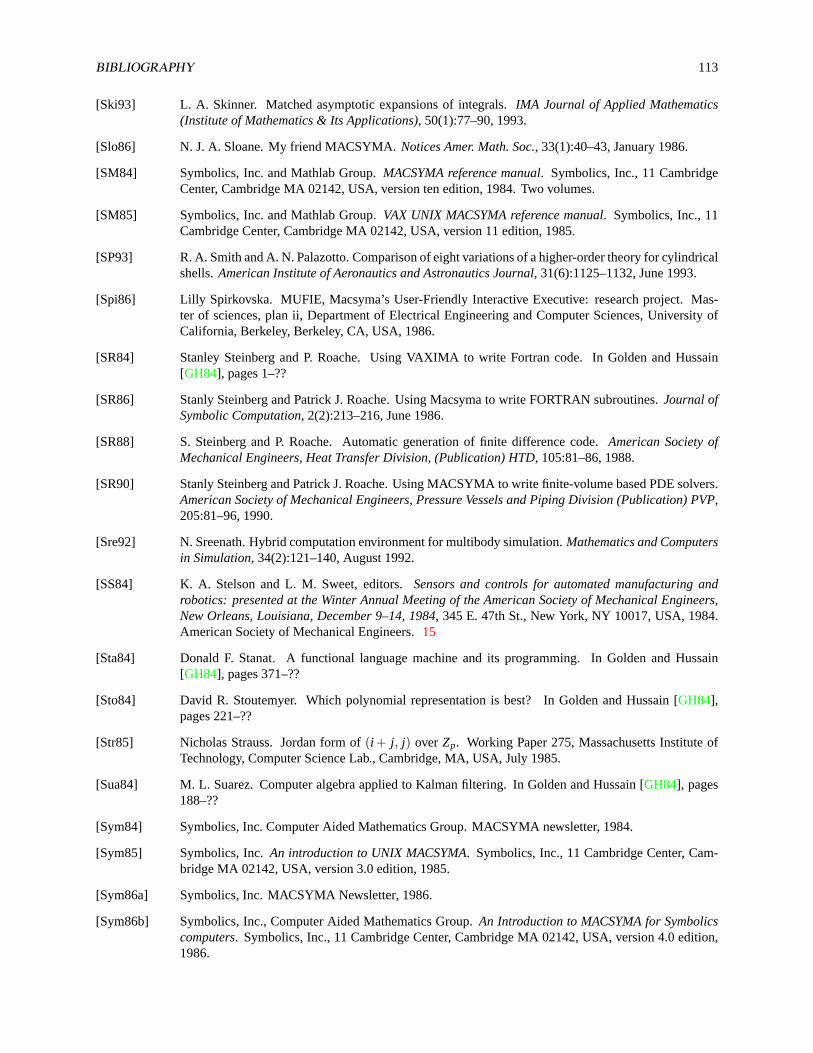
BIBLIOGRAPHY 113
[Ski93] L. A. Skinner. Matched asymptotic expansions of integrals.IMA Journal of Applied Mathematics(Institute of Mathematics & Its Applications), 50(1):77–90, 1993.
[Slo86] N. J. A. Sloane. My friend MACSYMA.Notices Amer. Math. Soc., 33(1):40–43, January 1986.
[SM84] Symbolics, Inc. and Mathlab Group.MACSYMA reference manual. Symbolics, Inc., 11 CambridgeCenter, Cambridge MA 02142, USA, version ten edition, 1984. Two volumes.
[SM85] Symbolics, Inc. and Mathlab Group.VAX UNIX MACSYMA reference manual. Symbolics, Inc., 11Cambridge Center, Cambridge MA 02142, USA, version 11 edition, 1985.
[SP93] R. A. Smith and A. N. Palazotto. Comparison of eight variations of a higher-order theory for cylindricalshells.American Institute of Aeronautics and Astronautics Journal, 31(6):1125–1132, June 1993.
[Spi86] Lilly Spirkovska. MUFIE, Macsyma’s User-Friendly Interactive Executive: research project. Mas-ter of sciences, plan ii, Department of Electrical Engineering and Computer Sciences, University ofCalifornia, Berkeley, Berkeley, CA, USA, 1986.
[SR84] Stanley Steinberg and P. Roache. Using VAXIMA to write Fortran code. In Golden and Hussain[GH84], pages 1–??
[SR86] Stanly Steinberg and Patrick J. Roache. Using Macsyma to write FORTRAN subroutines.Journal ofSymbolic Computation, 2(2):213–216, June 1986.
[SR88] S. Steinberg and P. Roache. Automatic generation of finite difference code.American Society ofMechanical Engineers, Heat Transfer Division, (Publication) HTD, 105:81–86, 1988.
[SR90] Stanly Steinberg and Patrick J. Roache. Using MACSYMA to write finite-volume based PDE solvers.American Society of Mechanical Engineers, Pressure Vessels and Piping Division (Publication) PVP,205:81–96, 1990.
[Sre92] N. Sreenath. Hybrid computation environment for multibody simulation.Mathematics and Computersin Simulation, 34(2):121–140, August 1992.
[SS84] K. A. Stelson and L. M. Sweet, editors.Sensors and controls for automated manufacturing androbotics: presented at the Winter Annual Meeting of the American Society of Mechanical Engineers,New Orleans, Louisiana, December 9–14, 1984, 345 E. 47th St., New York, NY 10017, USA, 1984.American Society of Mechanical Engineers.15
[Sta84] Donald F. Stanat. A functional language machine and its programming. In Golden and Hussain[GH84], pages 371–??
[Sto84] David R. Stoutemyer. Which polynomial representation is best? In Golden and Hussain [GH84],pages 221–??
[Str85] Nicholas Strauss. Jordan form of(i + j, j) over Zp. Working Paper 275, Massachusetts Institute ofTechnology, Computer Science Lab., Cambridge, MA, USA, July 1985.
[Sua84] M. L. Suarez. Computer algebra applied to Kalman filtering. In Golden and Hussain [GH84], pages188–??
[Sym84] Symbolics, Inc. Computer Aided Mathematics Group. MACSYMA newsletter, 1984.
[Sym85] Symbolics, Inc.An introduction to UNIX MACSYMA. Symbolics, Inc., 11 Cambridge Center, Cam-bridge MA 02142, USA, version 3.0 edition, 1985.
[Sym86a] Symbolics, Inc. MACSYMA Newsletter, 1986.
[Sym86b] Symbolics, Inc., Computer Aided Mathematics Group.An Introduction to MACSYMA for Symbolicscomputers. Symbolics, Inc., 11 Cambridge Center, Cambridge MA 02142, USA, version 4.0 edition,1986.
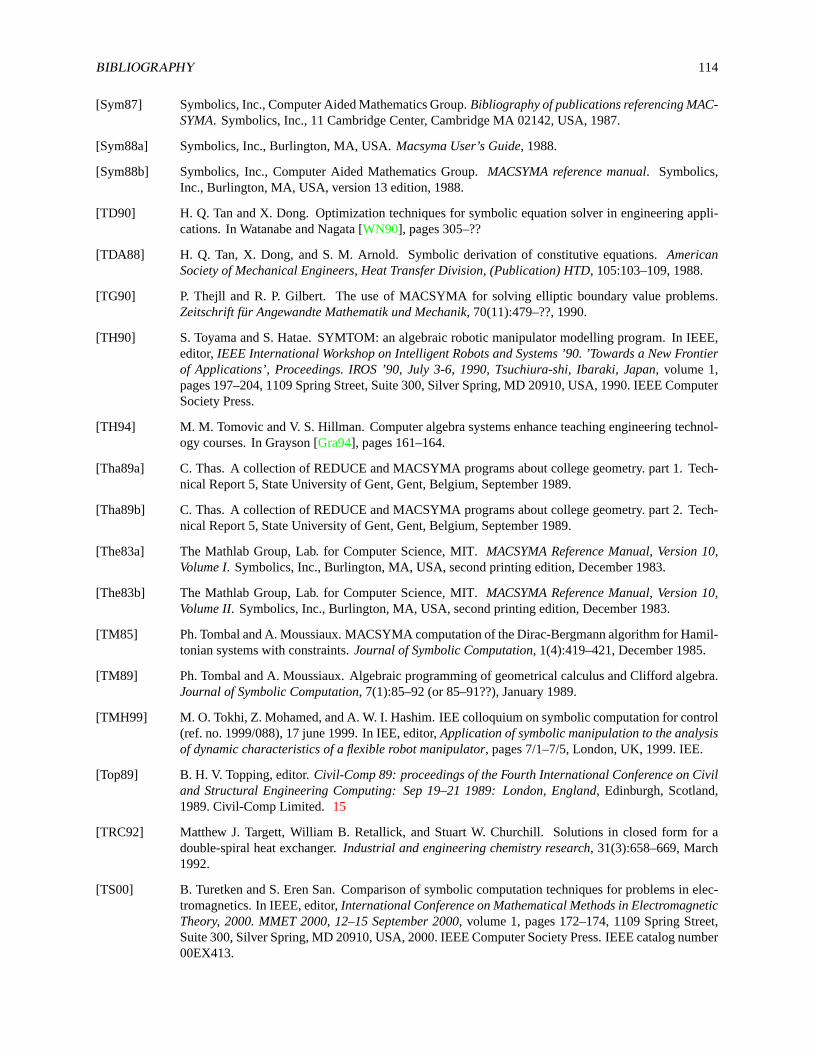
BIBLIOGRAPHY 114
[Sym87] Symbolics, Inc., Computer Aided Mathematics Group.Bibliography of publications referencing MAC-SYMA. Symbolics, Inc., 11 Cambridge Center, Cambridge MA 02142, USA, 1987.
[Sym88a] Symbolics, Inc., Burlington, MA, USA.Macsyma User’s Guide, 1988.
[Sym88b] Symbolics, Inc., Computer Aided Mathematics Group.MACSYMA reference manual. Symbolics,Inc., Burlington, MA, USA, version 13 edition, 1988.
[TD90] H. Q. Tan and X. Dong. Optimization techniques for symbolic equation solver in engineering appli-cations. In Watanabe and Nagata [WN90], pages 305–??
[TDA88] H. Q. Tan, X. Dong, and S. M. Arnold. Symbolic derivation of constitutive equations.AmericanSociety of Mechanical Engineers, Heat Transfer Division, (Publication) HTD, 105:103–109, 1988.
[TG90] P. Thejll and R. P. Gilbert. The use of MACSYMA for solving elliptic boundary value problems.Zeitschrift für Angewandte Mathematik und Mechanik, 70(11):479–??, 1990.
[TH90] S. Toyama and S. Hatae. SYMTOM: an algebraic robotic manipulator modelling program. In IEEE,editor,IEEE International Workshop on Intelligent Robots and Systems ’90. ’Towards a New Frontierof Applications’, Proceedings. IROS ’90, July 3-6, 1990, Tsuchiura-shi, Ibaraki, Japan, volume 1,pages 197–204, 1109 Spring Street, Suite 300, Silver Spring, MD 20910, USA, 1990. IEEE ComputerSociety Press.
[TH94] M. M. Tomovic and V. S. Hillman. Computer algebra systems enhance teaching engineering technol-ogy courses. In Grayson [Gra94], pages 161–164.
[Tha89a] C. Thas. A collection of REDUCE and MACSYMA programs about college geometry. part 1. Tech-nical Report 5, State University of Gent, Gent, Belgium, September 1989.
[Tha89b] C. Thas. A collection of REDUCE and MACSYMA programs about college geometry. part 2. Tech-nical Report 5, State University of Gent, Gent, Belgium, September 1989.
[The83a] The Mathlab Group, Lab. for Computer Science, MIT.MACSYMA Reference Manual, Version 10,Volume I. Symbolics, Inc., Burlington, MA, USA, second printing edition, December 1983.
[The83b] The Mathlab Group, Lab. for Computer Science, MIT.MACSYMA Reference Manual, Version 10,Volume II. Symbolics, Inc., Burlington, MA, USA, second printing edition, December 1983.
[TM85] Ph. Tombal and A. Moussiaux. MACSYMA computation of the Dirac-Bergmann algorithm for Hamil-tonian systems with constraints.Journal of Symbolic Computation, 1(4):419–421, December 1985.
[TM89] Ph. Tombal and A. Moussiaux. Algebraic programming of geometrical calculus and Clifford algebra.Journal of Symbolic Computation, 7(1):85–92 (or 85–91??), January 1989.
[TMH99] M. O. Tokhi, Z. Mohamed, and A. W. I. Hashim. IEE colloquium on symbolic computation for control(ref. no. 1999/088), 17 june 1999. In IEE, editor,Application of symbolic manipulation to the analysisof dynamic characteristics of a flexible robot manipulator, pages 7/1–7/5, London, UK, 1999. IEE.
[Top89] B. H. V. Topping, editor.Civil-Comp 89: proceedings of the Fourth International Conference on Civiland Structural Engineering Computing: Sep 19–21 1989: London, England, Edinburgh, Scotland,1989. Civil-Comp Limited. 15
[TRC92] Matthew J. Targett, William B. Retallick, and Stuart W. Churchill. Solutions in closed form for adouble-spiral heat exchanger.Industrial and engineering chemistry research, 31(3):658–669, March1992.
[TS00] B. Turetken and S. Eren San. Comparison of symbolic computation techniques for problems in elec-tromagnetics. In IEEE, editor,International Conference on Mathematical Methods in ElectromagneticTheory, 2000. MMET 2000, 12–15 September 2000, volume 1, pages 172–174, 1109 Spring Street,Suite 300, Silver Spring, MD 20910, USA, 2000. IEEE Computer Society Press. IEEE catalog number00EX413.
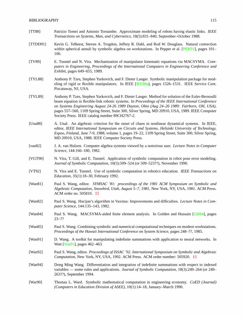
BIBLIOGRAPHY 115
[TT88] Patrizio Tomei and Antonio Tornambe. Approximate modeling of robots having elastic links.IEEETransactions on Systems, Man, and Cybernetics, 18(5):831–840, September–October 1988.
[TTDD91] Kevin G. TeBeest, Steven A. Trogdon, Jeffrey R. Dahl, and Rod W. Douglass. Natural convectionwithin spherical annuli by symbolic algebra on workstations. In Pepper et al. [PEK91], pages 101–106.
[TV89] E. Tunstel and N. Vira. Mechanization of manipulator kinematic equations via MACSYMA.Com-puters in Engineering, Proceedings of the International Computers in Engineering Conference andExhibit, pages 649–655, 1989.
[TYL88] Anthony P. Tzes, Stephen Yurkovich, and F. Dieter Langer. Symbolic manipulation package for mod-eling of rigid or flexible manipulators. In IEEE [IEE88a], pages 1526–1531. IEEE Service Cent.Piscataway, NJ, USA.
[TYL89] Anthony P. Tzes, Stephen Yurkovich, and F. Dieter Langer. Method for solution of the Euler-Bernoullibeam equation in flexible-link robotic systems. InProceedings of the IEEE International Conferenceon Systems Engineering August 24-26 1989 Dayton, Ohio (Aug 24–26 1989: Fairborn, OH, USA),pages 557–560, 1109 Spring Street, Suite 300, Silver Spring, MD 20910, USA, 1989. IEEE ComputerSociety Press. IEEE catalog number 89CH2767-2.
[Una88] A. Unal. An algebraic criterion for the onset of chaos in nonlinear dynamical systems. In IEEE,editor, IEEE International Symposium on Circuits and Systems, Helsinki University of Technology,Espoo, Finland, June 7-9, 1988, volume 1, pages 19–22, 1109 Spring Street, Suite 300, Silver Spring,MD 20910, USA, 1988. IEEE Computer Society Press.
[van82] J. A. van Hulzen. Computer algebra systems viewed by a notorious user.Lecture Notes in ComputerScience, 144:166–180, 1982.
[VGT90] N. Vira, T. Gill, and E. Tunstel. Application of symbolic computation in robot pose error modeling.Journal of Symbolic Computation, 10(5):509–524 (or 509–523??), November 1990.
[VT92] N. Vira and E. Tunstel. Use of symbolic computation in robotics education.IEEE Transactions onEducation, 35(1):18–30, February 1992.
[Wan81] Paul S. Wang, editor.SYMSAC ’81: proceedings of the 1981 ACM Symposium on Symbolic andAlgebraic Computation, Snowbird, Utah, August 5–7, 1981, New York, NY, USA, 1981. ACM Press.ACM order no. 505810.15
[Wan82] Paul S. Wang. Hacijan’s algorithm in Vaxima: Improvements and difficulties.Lecture Notes in Com-puter Science, 144:135–143, 1982.
[Wan84] Paul S. Wang. MACSYMA-aided finite element analysis. In Golden and Hussain [GH84], pages23–??
[Wan85] Paul S. Wang. Combining symbolic and numerical computational techniques on modern workstations.Proceedings of the Hawaii International Conference on System Science, pages 248–??, 1985.
[Wan91] D. Wang. A toolkit for manipulating indefinite summations with application to neural networks. InWatt [Wat91], pages 462–463.
[Wan92] Paul S. Wang, editor.Proceedings of ISSAC ’92. International Symposium on Symbolic and AlgebraicComputation, New York, NY, USA, 1992. ACM Press. ACM order number: 505920.15
[Wan94] Dong Ming Wang. Differentiation and integration of indefinite summations with respect to indexedvariables — some rules and applications.Journal of Symbolic Computation, 18(3):249–264 (or 249–263??), September 1994.
[War90] Thomas L. Ward. Symbolic mathematical computation in engineering economy.CoED (Journal)(Computers in Education Division of ASEE), 10(1):14–18, January–March 1990.
BIBLIOGRAPHY 116
[Wat91] Stephen M. Watt, editor.Proceedings of the 1991 International Symposium on Symbolic and AlgebraicComputation. ISSAC ’91, July 15–17, 1991, Bonn, Germany, New York, NY, USA, 1991. ACM Press.15
[Way90] Peter Wayner. Mainframe math on a PC: Macsyma, the grande dame of computer algebra, is finallyavailable for PCs.BYTE Magazine, 15(1):207–208, 210, January 1990.
[WH84] Ralph Wilcox and Leo Harten. Analytical solutions to some linear systems of differential equation. InGolden and Hussain [GH84], pages 138–??
[Whi77a] J. L. White. LISP: Data is program, a tutorial in LISP. In Fateman et al. [F+77], pages ??–??
[Whi77b] J. L. White. LISP: Program is data, a historical perspective on MACLISP. In Fateman et al. [F+77],pages ??–??
[WKB86] S. J. Watowich, J. L. Krause, and R. S. Berry. Stability analysis of an optimally controlled light-drivenengine.Journal of Symbolic Computation, 2(1):103–108, March 1986.
[WN90] Shunro Watanabe and Morio Nagata, editors.ISSAC ’90: proceedings of the International Symposiumon Symbolic and Algebraic Computation: August 20–24, 1990, Tokyo, Japan, New York, NY, USAand Reading, MA, USA, 1990. ACM Press and Addison-Wesley.15
[Wol79] Steve Wolfram. MACSYMA tools for Feynman diagram calculations. In Lewis [Lew79], pages ??–??
[Wol84] Steve Wolfram. Five years of SMP. In Golden and Hussain [GH84], pages 220–??
[Woo84] David L. Wood. An overdetermined system of partial differential equations. In Golden and Hussain[GH84], pages 121–??
[WS83] Michael Wester and Stanly Steinberg. An extension to MACSYMA’s concept of functional differenti-ation. SIGSAM Bulletin, 17(3/4):25–30, August/November 1983.
[WS84] Michael Wester and Stanly Steinberg. A survey of symbolic differentiation implementations. InGolden and Hussain [GH84], pages 330–??
[WS88] C. F. Weggel and D. P. Schwartz. New analytical formulas for calculating magnetic field.IEEETransactions on Magnetics, 24(2 (part 2)):1544–1547, March 1988.
[WS91a] D. Wang and B. Schurmann. Computer aided investigations of artificial neural systems. In IEEE,editor,International Joint Conference on Neural Networks, 1991., IJCNN-91-Seattle, 8–14 July 1991,volume 2, pages 981–981, 1109 Spring Street, Suite 300, Silver Spring, MD 20910, USA, 1991. IEEEComputer Society Press.
[WS91b] Dongming Wang and Bernd Schurmann. Computer aided investigations of artificial neural systems.In IEEE [IEE91], pages 2325–2330. Three volumes. IEEE catalog number 91CH3065-0.
[WS92] D. Wang and B. Schurmann. Computer aided analysis and derivation for artificial neural systems.IEEE Transactions on Software Engineering, 18(8):728–735, August 1992.
[Yag84] J. J. Yagla. Stability criteria for finite difference equations. In Golden and Hussain [GH84], pages294–??
[YP91] Robert J. Yamartino and Richard Pavelle. An application of computer algebra to a problem in stratifiedfluid flow. Journal of Symbolic Computation, 12(6):669–672, December 1991.
[yS88] Chiung yu Syu. An application of MACSYMA in fluid mechanics. Thesis (m.s.m.e.), University ofMassachusetts at Amherst, Amherst, MA, USA, 1988.
[YW85] Douglas A. Young and Paul S. Wang. An improved plotting package for Vaxima. In Buchberger[Buc85], page 431.

BIBLIOGRAPHY 117
[YW87] D. A. Young and P. S. Wang. GI/S: a graphical user interface for symbolic computation systems.Journal of Symbolic Computation, 4(3):365–380, December 1987.
[ZZ86] S. W. Zewari and J. M. Zugel. Prolog implementation in robot kinematics. In Gupta et al. [GA+86],pages 133–136. Three volumes.