The introduction to learning Poisson/Superfish & Astra codes

Sara ZareiWinter 96

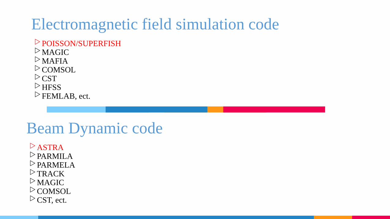
Electromagnetic field simulation code▷POISSON/SUPERFISH▷MAGIC▷MAFIA▷COMSOL▷CST▷HFSS▷FEMLAB, ect.

Beam Dynamic code▷ASTRA▷PARMILA▷PARMELA▷TRACK▷MAGIC▷COMSOL▷CST, ect.

Poisson Superfish

Los Alamos National Laboratory1976

Introduction I

▷ a collection of programs forcalculating static magnetic andelectric fields and radio-frequencyelectromagnetic fields in either 2-DCartesian coordinates or axiallysymmetric cylindrical coordinates.

▷ Getting Started with PoissonSuperfish: The best way to learnabout Poisson Superfish is to run thesample problems described in thedocumentation.

SFTOC.DOC This file, containing the table of contents and suggestions for viewing and

printing.

SFINTRO.DOC General information about the software installation, features in the codes,

references, history, SF.INI configuration, and technical support.

SFFILES.DOC Brief descriptions of all the input and output files used in the Poisson

Superfish codes.

SFCODES.DOC Information about the main programs Autofish, Automesh, Fish, CFish,

Poisson, and Pandira.

SFPOSTP.DOC Information about the postprocessor programs WSFplot, SFO, SF7, and

Force.

SFCODES2.DOC The automated tuning programs CCLfish, CDTfish, DTLfish, MDTfish,

ELLfish, and RFQfish.

SFCODES3.DOC General purpose plotting programs Quikplot and Tablplot, and utility

programs Beta, Kilpat, List35, ConvertF, SF8, FScale, SegField, and

SFOtable.

SFEXMPL1.DOC Discussion of rf-field example files for Fish, CFish, and Autofish contained

in the Examples\RadioFrequency subdirectories.

SFEXMPL2.DOC Discussion of the static-field example files for Poisson and Pandira

contained in the Examples\Magnetostatic and Examples\Electrostatic

subdirectories.

SFEXMPL3.DOC Discussion of the tuning-program example files contained in the

Examples\CavityTuning subdirectories.

SFPHYS1.DOC Theory of electrostatics and magnetostatics from John Warren’s treatment in

the 1987 Reference Manual

SFPHYS2.DOC Properties of static magnetic and electric fields from John Warren’s

treatment in the 1987 Reference Manual

SFPHYS3.DOC Boundary conditions and symmetries from John Warren’s treatment in the

1987 Reference Manual

SFPHYS4.DOC Numerical methods in Poisson and Pandira from John Warren’s treatment in

the 1987 Reference Manual

SFPHYS5.DOC RF cavity theory from John Warren’s treatment in the 1987 Reference

Manual

Example

Theory

Codes

description

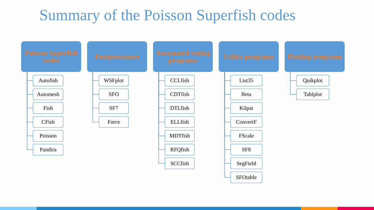
Summary of the Poisson Superfish codes

Poisson Superfishcodes

Autofish

Automesh

Fish

CFish

Poisson

Pandira

Postprocessors

WSFplot

SFO

SF7

Force

Automated tuning programs

CCLfish

CDTfish

DTLfish

ELLfish

MDTfish

RFQfish

SCCfish

Utility programs

List35

Beta

Kilpat

ConvertF

FScale

SF8

SegField

SFOtable

Plotting programs

Quikplot

Tablplot

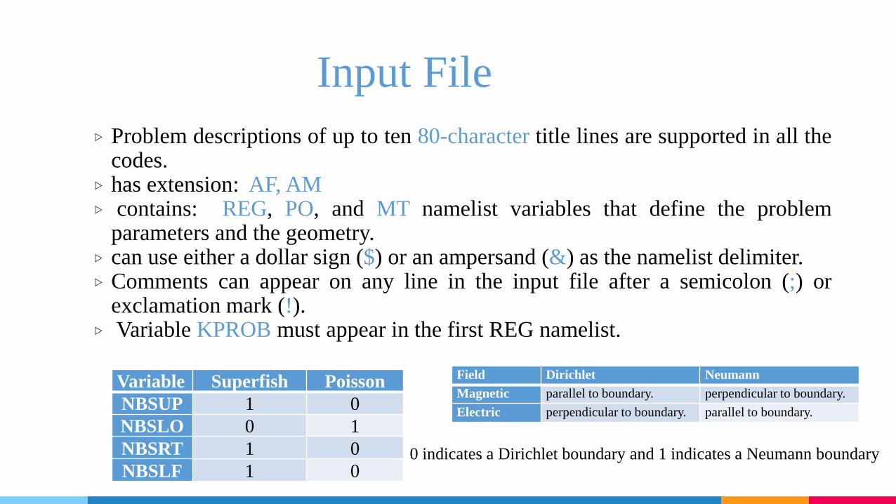
Input File

▷ Problem descriptions of up to ten 80-character title lines are supported in all thecodes.

▷ has extension: AF, AM▷ contains: REG, PO, and MT namelist variables that define the problem

parameters and the geometry.▷ can use either a dollar sign ($) or an ampersand (&) as the namelist delimiter.▷ Comments can appear on any line in the input file after a semicolon (;) or

exclamation mark (!).▷ Variable KPROB must appear in the first REG namelist.

Variable Superfish Poisson

NBSUP 1 0

NBSLO 0 1

NBSRT 1 0

NBSLF 1 00 indicates a Dirichlet boundary and 1 indicates a Neumann boundary

Field Dirichlet Neumann

Magnetic parallel to boundary. perpendicular to boundary.

Electric perpendicular to boundary. parallel to boundary.

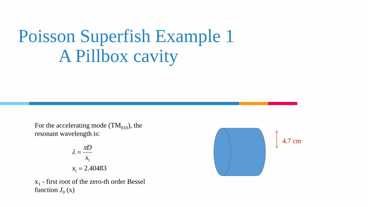
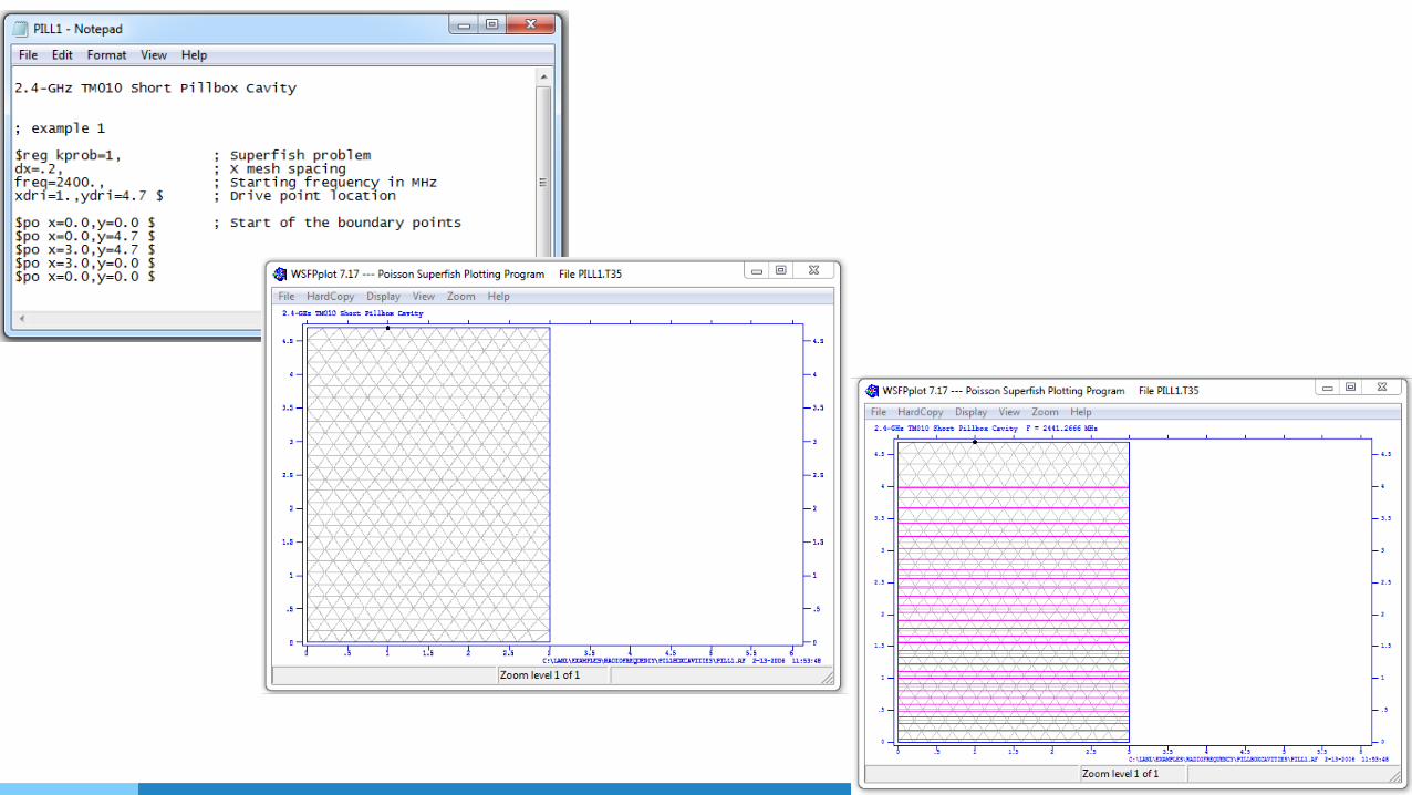
Poisson Superfish Example 1A Pillbox cavity

For the accelerating mode (TM010), the

resonant wavelength is:

40483.21

1

x

x

D

x1 - first root of the zero-th order Bessel

function J0 (x)

4.7 cm

SF 7

SFO

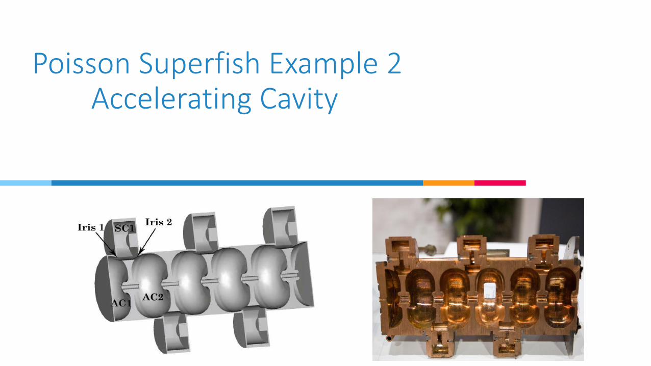
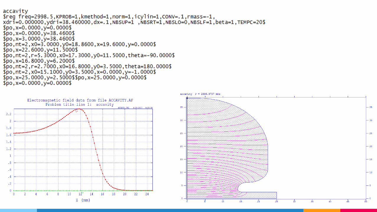
Poisson Superfish Example 2Accelerating Cavity

AstraA Space Charge Tracking Algorithm

DESY1997

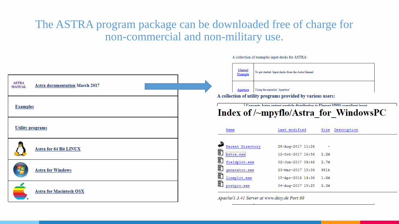
The ASTRA program package can be downloaded free of charge for non-commercial and non-military use.

Introduction I

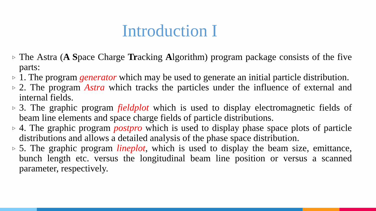
▷ The Astra (A Space Charge Tracking Algorithm) program package consists of the fiveparts:

▷ 1. The program generator which may be used to generate an initial particle distribution.▷ 2. The program Astra which tracks the particles under the influence of external and

internal fields.▷ 3. The graphic program fieldplot which is used to display electromagnetic fields of

beam line elements and space charge fields of particle distributions.▷ 4. The graphic program postpro which is used to display phase space plots of particle

distributions and allows a detailed analysis of the phase space distribution.▷ 5. The graphic program lineplot, which is used to display the beam size, emittance,

bunch length etc. versus the longitudinal beam line position or versus a scannedparameter, respectively.

Introduction II

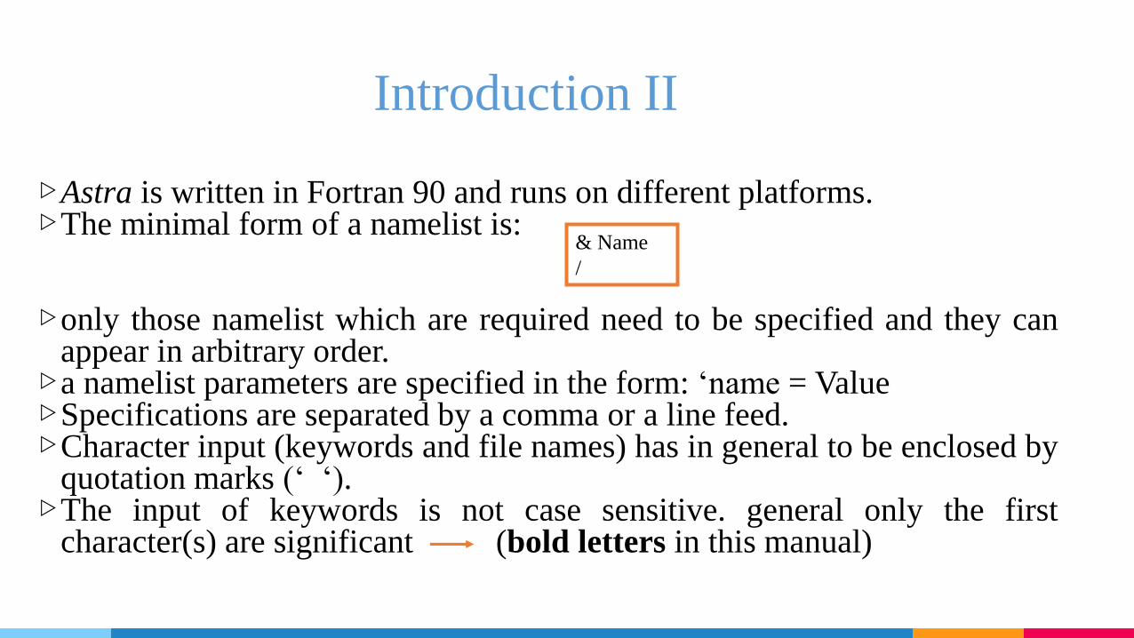
▷Astra is written in Fortran 90 and runs on different platforms.▷The minimal form of a namelist is:

▷only those namelist which are required need to be specified and they canappear in arbitrary order.▷a namelist parameters are specified in the form: ‘name = Value▷Specifications are separated by a comma or a line feed.▷Character input (keywords and file names) has in general to be enclosed by

quotation marks (‘ ‘).▷The input of keywords is not case sensitive. general only the first

character(s) are significant (bold letters in this manual)

& Name

/

Definition of the initial particle distribution

▷distribution file name should end with the extension ‘.ini’ or with ‘.zpos.run’. zpos =four digit number & run = three digit number specifying the run number▷Mix different kinds of particles as an initial particle distribution

input particle distribution

program generator user written programoutput distribution of Astra

(except Local_emit = T)

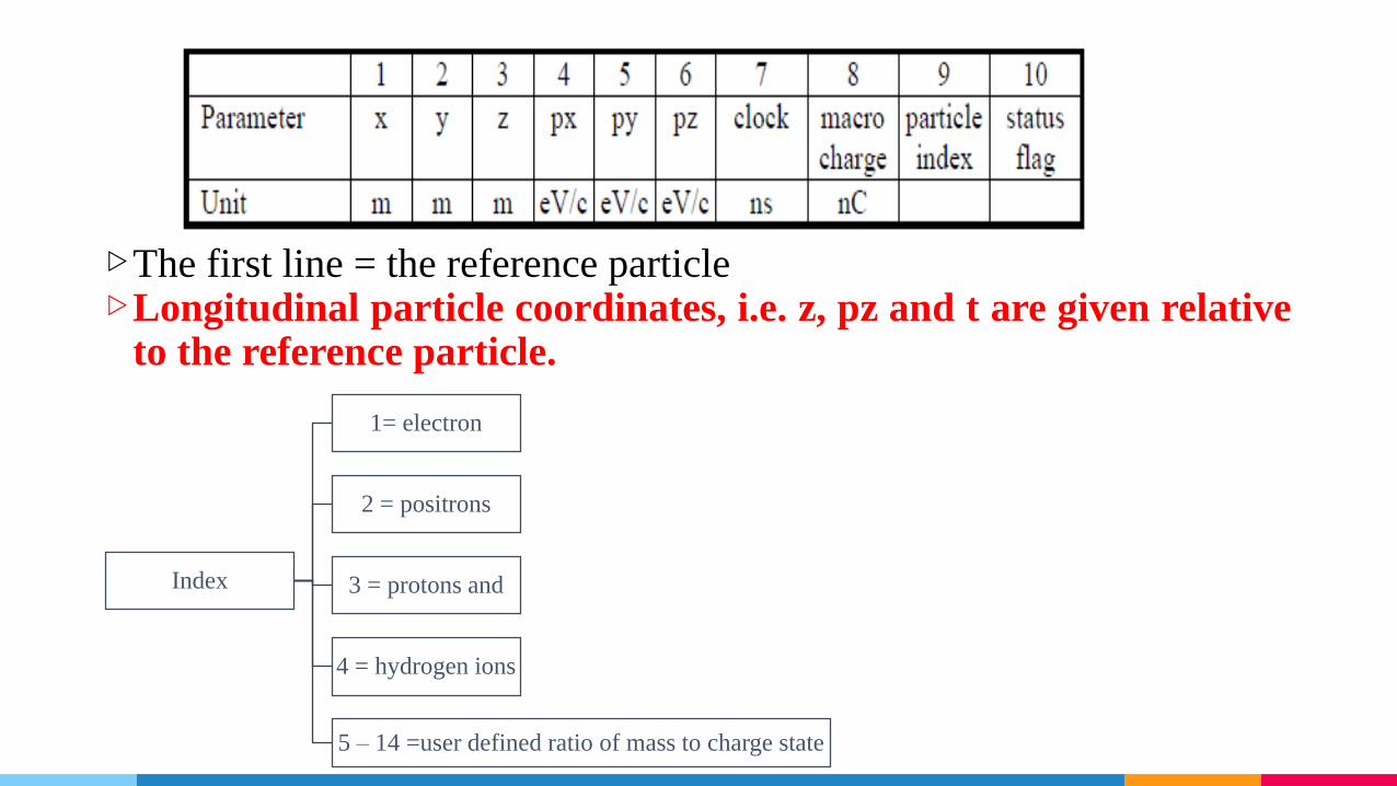
▷The first line = the reference particle▷Longitudinal particle coordinates, i.e. z, pz and t are given relative

to the reference particle.

Index

1= electron

2 = positrons

3 = protons and

4 = hydrogen ions

5 – 14 =user defined ratio of mass to charge state

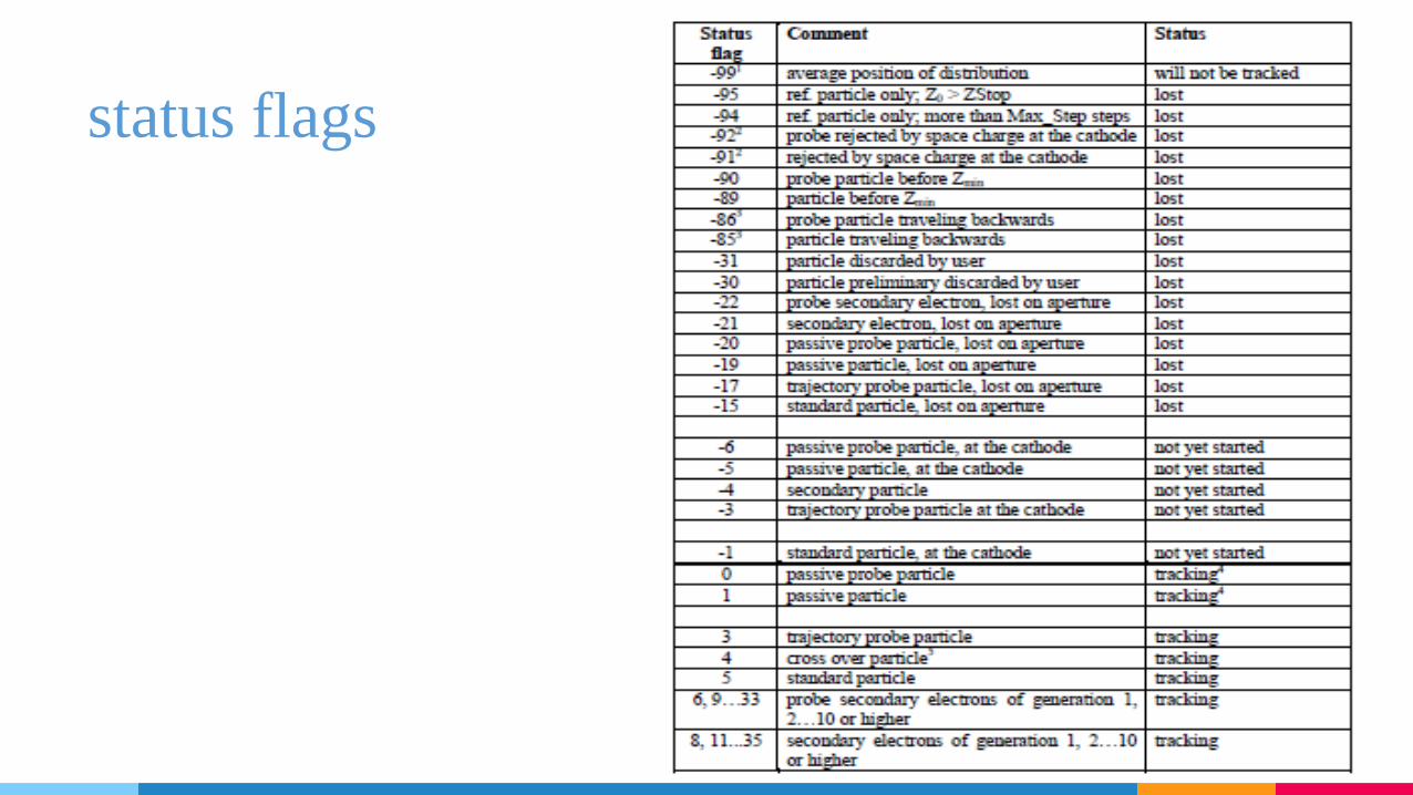
status flags

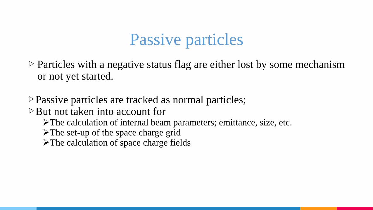
Passive particles

▷ Particles with a negative status flag are either lost by some mechanismor not yet started.

▷Passive particles are tracked as normal particles;▷But not taken into account for

The calculation of internal beam parameters; emittance, size, etc.The set-up of the space charge gridThe calculation of space charge fields

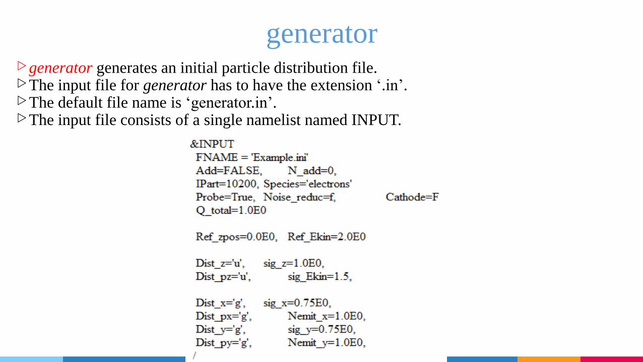
generator▷generator generates an initial particle distribution file.▷The input file for generator has to have the extension ‘.in’.▷The default file name is ‘generator.in’.▷The input file consists of a single namelist named INPUT.

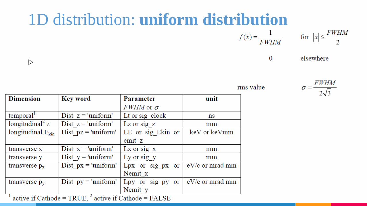
1D distribution: uniform distribution

▷

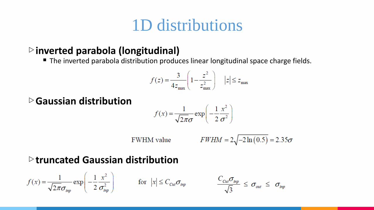
1D distributions

▷ inverted parabola (longitudinal) The inverted parabola distribution produces linear longitudinal space charge fields.

▷Gaussian distribution

▷ truncated Gaussian distribution

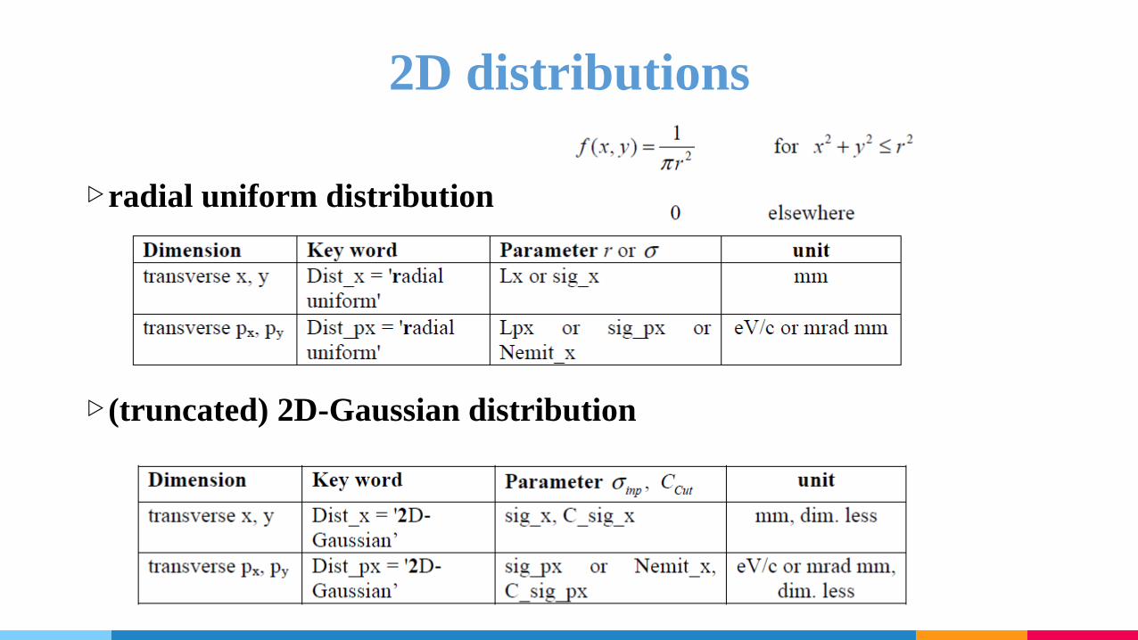
2D distributions

▷radial uniform distribution

▷ (truncated) 2D-Gaussian distribution

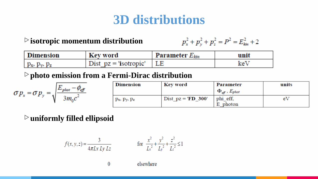
3D distributions

▷ isotropic momentum distribution

▷photo emission from a Fermi-Dirac distribution

▷uniformly filled ellipsoid

CAVITY I▷RF, static electric and magnetic fields and fields generated by linear

plasmas.▷cavity fields may be generated by analytical calculations,

measurements or numerical codes.▷ field table z-position (column 1 in m) & longitudinal on-axiselectric field amplitude (column 2 in arbitrary units)▷The transverse field components are calculated from the derivatives of

the on-axis field.▷The polynomial expansion extends to 1st order or 3st order .▷The polynomial expansion is perfect already in first order for a pure

sine-like spatial wave.

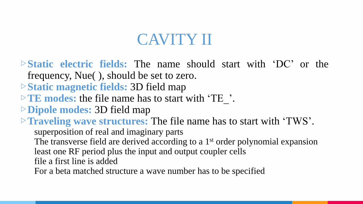
CAVITY II

▷Static electric fields: The name should start with ‘DC’ or thefrequency, Nue( ), should be set to zero.▷Static magnetic fields: 3D field map▷TE modes: the file name has to start with ‘TE_’.▷Dipole modes: 3D field map▷Traveling wave structures: The file name has to start with ‘TWS’.

superposition of real and imaginary partsThe transverse field are derived according to a 1st order polynomial expansionleast one RF period plus the input and output coupler cellsfile a first line is addedFor a beta matched structure a wave number has to be specified