0

Master Thesis

Master in Economics & Business – International Economics

The Impact of Trade Liberalization on the Aggregate Financial

Performance of Firms

A Theoretical and an Empirical Analysis of the Role of Resource, Market Share and Profit

Reallocations in Eastern Europe and Central Asia

ERASMUS UNIVERSITY ROTTERDAM

Erasmus School of Economics

Department of Economics

International Economics

Supervisor: Dr. Julian Emami Namini

Jasper Olivier van Schaik

Student Number: 325683

Contact Details: vanschaik.jasper@gmail.com

Submitted on: 20th of July 2012

1

Abstract

This research paper theoretically and empirically investigates the role of resource, market share and

profit reallocations in explaining the impact of trade liberalization on the aggregate performance of

firms. A theoretical model, which is largely based on the model by Melitz (2003) and incorporates

firm heterogeneity in the total factor productivity parameter, argues that the financial performance of

firms can be used as an accurate proxy for productivity. The theoretical results suggest a positive

impact of trade liberalization on the sector-wide aggregate financial performance of all firms active in

an industry, but an insignificant impact of trade liberalization on the average performance of exporters.

The empirical analysis, employing firm level data on 27 Eastern European and Central Asian countries

over the period 2002-2009, confirms the theoretical predictions. In particular, it is shown that,

independent of the different dependent variables used and the econometric estimation procedures

followed, trade liberalization has a significantly positive impact on the sector-wide average financial

performance of firms. Additionally, it is proven that among exporters, trade liberalization does not

have a significant impact on aggregate performance.

JEL Classification: F12, F15, F41, F43, O11, O41

Keywords: Trade Liberalization, Productivity, Economic Growth, Imperfect Competition, Firm

Heterogeneity in the Total Factor Productivity Parameter

2

Table of Contents

Abstract page 1

1. Introduction page 3

2. Literature Review page 6

2.1 Theoretical Literature page 6

2.2 Empirical Literature page 8

3. The Theoretical Analysis page 11

3.1 Setup of the Model page 11

3.2 Firm Entry and Exit page 15

3.3 Equilibrium in a Closed Economy page 17

3.4 Equilibrium in an Open Economy page 19

3.5 Overview of the Theoretical Results page 26

4. The Empirical Analysis page 27

4.1 Hypotheses page 27

4.2 Data page 27

4.3 Methodology page 36

4.4 Empirical Results page 39

4.5 Trade Liberalization and Performance: A Different Perspective page 53

4.6 Overview of the Empirical Results page 55

5. Conclusion page 57

6. References page 59

7. Appendix page 61

3

1 Introduction

Europe is in a financial and a political crisis. Financially, Europe is suffering from the large fiscal

deficits encountered by Southern European countries and a highly fragile international financial

system, which both put the stability of the common currency, the Euro (€), at risk. Politically, Europe

is suffering from many conflicts of interest due to the high degree of economic, financial and political

heterogeneity across European Union (EU) member states. Countries have their own strengths and

weaknesses and, accordingly, their own economic and political problems and priorities. Discontent

over Europe’s economic performance, with an average real economic growth rate close to only half a

percent, is the biggest factor hampering the implementation of an effective solution for the current

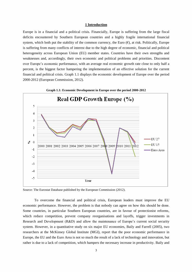
financial and political crisis. Graph 1.1 displays the economic development of Europe over the period

2000-2012 (European Commission, 2012).

Graph 1.1: Economic Development in Europe over the period 2000-2012

Source: The Eurostat Database published by the European Commission (2012).

To overcome the financial and political crisis, European leaders must improve the EU

economic performance. However, the problem is that nobody can agree on how this should be done.

Some countries, in particular Southern European countries, are in favour of protectionist reforms,

which reduce competition, prevent company reorganisations and layoffs, trigger investments in

Research and Development (R&D) and allow the maintenance of Europe’s current social security

system. However, in a quantitative study on six major EU economies, Baily and Farrell (2005), two

researchers at the McKinsey Global Institute (MGI), report that the poor economic performance in

Europe, the EU and the Euro Area is not so much the result of a lack of technology and innovation, but

rather is due to a lack of competition, which hampers the necessary increase in productivity. Baily and

4

Farrell (2005) emphasize the necessity of regulatory reforms, which boost competition, as they can

improve productivity by triggering firms to make smart and innovative investments. Firms that do so

successfully manage to perform better, expand their market shares and employ more workers. Less

productive firms are confronted with a dilemma of either improving their businesses, which is costly,

or exiting the market. Trade liberalization and the elimination of artificial protectionist laws and trade

barriers are considered as important steps towards a market increasingly determined by competitive

forces. Baily and Farrell (2005) conclude that classic, open economy and competitive market

mechanisms have a positive and structural impact on European economies by boosting the main

drivers of economic growth and allow Europe to overcome the current financial and political crisis

without abandoning its well-developed social security system.

The suggestion that classic, open economy and competitive market mechanisms have a

positive impact on firm and aggregate productivity serves as the main motivation for formally

studying and quantifying the impact of trade liberalization on the sector-wide average performance of

firms. There are many channels through which trade liberalization can affect productivity and

performance, including economies of scale, knowledge spillovers and innovative incentives. This

research paper will, in line with the quantitative assertions by Baily and Farrell (2005), primarily

investigate the role of resource, market share and profit reallocations from less to more productive

firms in explaining the influence of trade liberalization on aggregate performance. To this end, this

paper presents a theoretical and an empirical analysis of the aforementioned relationship.

The theoretical analysis largely builds upon the model by Melitz (2003), which assesses the

role of trade liberalization as a catalyst for inter-firm resource, market share and profit reallocations

within an industry. The theoretical model developed in this paper incorporates many of the features of

the model by Melitz (2003) and, in addition to Melitz (2003), argues that firm productivity can

objectively be proxied by indicators of financial performance. In particular, it is shown that there is a

direct positive relationship between the sector-wide average financial performance of firms and the

aggregate productivity, which supports the idea that financial performance is a reliable, objective and

accurately measurable proxy of productivity. The theoretical results in this paper suggest that trade

liberalization has a positive influence on the industry-wide average productivity and financial

performance level through processes of resource, market share and profit reallocations from less to

more productive firms. Among exporting firms, it is shown that trade liberalization does not have a

significant impact on the sector-wide average financial performance.

The theoretical results are used to formulate two hypotheses, which are tested empirically in

this paper. The empirical analysis employs firm level data on 27 Eastern European and Central Asian

countries over the period 2002-2009, provided by the Business Environment and Enterprise

Performance Surveys (BEEPS) and constructed by the joint effort of the World Bank and the

European Bank for Reconstruction and Development. The information gathered covers many different

aspects of a firm, including general information, infrastructure and services, sales and supplies, the

degree of competition, capacity, land and permits, crime, finance, business-government relations,

labour, the business environment, and performance. The panel regression results, based on different

model specifications and the implementation of various fixed effects estimation techniques, confirm

the hypotheses formulated on the basis of the theoretical analysis. In particular, the outcomes reveal a

stable, robust and significantly positive impact of the sector-wide export intensity on the industry-wide

5

average financial performance, which suggests that trade liberalization has a positive influence on the

aggregate performance of firms. Additionally, it is shown that there is an insignificant relationship

between the sector-wide average export intensity and the aggregate financial performance of exporters,

which supports the theoretical hypothesis that trade liberalization has no impact on the average

performance of exporters. These two outcomes support the idea that sector-wide improvements in

financial performance are the result of inter-firm resource, market share and profit reallocations

towards more efficient, mainly exporting firms within an industry. Overall, the results prove the

significant importance of resource, market share and profit reallocations from less to more productive

firms in explaining the positive influence of trade liberalization on the industry-wide average

performance of firms and, accordingly, country-wide welfare.

The remainder of this paper is structured as follows. An overview of the existing theoretical

and empirical literature on the impact of trade liberalization on productivity is presented in section 2.

Attention is also paid to the underlying mechanisms explaining the relationship. Section 3 presents a

theoretical analysis of the link between trade liberalization and the sector-wide average productivity

and financial performance, using a model that largely builds upon the pioneering research by Melitz

(2003) and serving as a framework for the formulation of empirical hypotheses. The model focuses on

the role of resource, market share and profit reallocations in explaining the influence of trade

liberalization on the industry-wide average performance of firms. Section 4 deals with the empirical

analysis, employing a panel regression setup and a sample of 27 Eastern European and Central Asian

countries to study the importance of resource, market share and profit reallocations in explaining the

impact of trade liberalization on the aggregate financial performance. Section 5 concludes.

6

2 Literature Review

Many economists have studied the impact of trade liberalization on firm performance, both from a

theoretical and an empirical point of view. In most cases, performance is assessed and estimated on the

basis of plant-level total factor productivity.

2.1 Theoretical Literature

Theoretically, economists have stressed the positive impact of trade liberalization on firm productivity

through a variety of channels. Grossman and Helpman (1991, 1993) analytically emphasize the

importance of knowledge spillover effects resulting from international trade of final and intermediate

products by means of a very simple and intuitive model. Production of different products takes place

with the help of land, labour, and knowledge capital, which is a public input factor. It is assumed that

knowledge accumulates as a by-product of production experience and is completely external to an

individual manufacturing firm. The general equilibrium outcome indicates that trade liberalization

improves plant-specific productivity through triggering innovations and access to a wider variety of

more advanced intermediate inputs and capital goods. Using these products and absorbing the more

advanced knowledge required to produce these kind of goods constitutes a process of technology

diffusion, allowing firms to update their production processes and capital stock. This, logically, has a

positive influence on plant performance, productivity, and economic growth.

Aghion et al. (2005) focus on a firm’s response in terms of innovative investments to the entry

threat of foreign firms imposed by trade liberalization. The researchers develop an adjusted version of

the Schumpeterian discrete-time model, assuming that a final good is manufactured by a competitive

industry using a continuum of intermediate goods, which are transformed by a technology and

productivity parameter. This technology and productivity parameter measures the quality of the inputs

and, thus, determines how much of these inputs needs to be used in production. The equilibrium

innovation investment level is determined on the basis of a relatively simple and straightforward profit

maximization exercise. The solution indicates that more advanced domestic firms will be encouraged

to invest more in innovation following the increased entry threat of foreign firms due to trade

liberalization. Less advanced firms, though, will be disincentivized to innovate, as their chance of

outperforming the foreign entrant is minimal. The consequently lower profits and market shares will

force these firms to exit the market. Overall, the model indicates that trade liberalization has a positive

effect on the surviving firms in the market through increased incentives to invest in innovation.

Goh (2000) emphasizes the importance of a fairly similar mechanism in explaining the

economic impacts of trade liberalization as the mechanism presented by Aghion et al. (2005). The

researcher explains the positive influence of trade liberalization on firm productivity through the

concepts of technological effort and opportunity costs. In particular, it is assumed that adopting new,

more efficient technologies is a time-consuming process, yielding forgone profits and thus an

opportunity cost. The model is based on an inverse relationship between the time spent on

technological search and the cost of production and follows a two-stage maximization setup. In the

first stage, the firm determines the optimal time spent on technological search. In the second stage, the

firm decides upon the optimal production level, given the technological search time and the

accompanying cost of production. The model is solved by backward induction. In particular, the firm’s

7

optimal time spent on technological search is based on a trade-off between marginal benefits,

consisting of a strategic effect and an efficiency effect, and marginal costs, being the opportunity cost

effect of technological effort. The researcher shows that international protection in the form of tariffs

and quota unambiguously reduces technological search effort due to higher opportunity costs. Namely,

in a protected environment, firms will always be able to serve a larger share of the market and earn

higher profits. Trade liberalization, however, tends to reduce this opportunity cost and to increase

technological effort, efficiency, and productivity under the commonly made assumptions of linear

marginal costs and demand functions.

Holmes and Schmitz (2001) assess the link between trade liberalization and firm productivity

by developing a theoretical model used to evaluate the time firms devote to productive and

unproductive entrepreneurial activities. The researchers develop an adjusted version of the model by

Grossman and Helpman (1991), described earlier. It assumes the existence of two firms, competing in

a technology ladder setup. The firms can divide their available time between two activities,

determining their ladder positions, namely research and attempts to block the innovative practices of

rivals. Solving the model, which is characterized by various scenarios in terms of technology ladder

positions, is based on a three step procedure. The main result derived indicates that trade liberalization,

i.e. ‘an improvement in the state of trade’ as it is referred to in the article, shifts the time spent on

unproductive activities towards productive activities as the relative returns change in favour of

research. This conclusion indicates a clear firm productivity improvement and holds for reductions in

domestic as well as foreign tariffs.

Trade is often said to give rise to scale economies, improving productivity of firms. Tybout

and Westbrook (1995) provide an overview of the sources of economies of scale that, through

increased openness to trade, improve efficiency. Increased production due to foreign sales

opportunities give rise to increasing returns to scale by spreading sunk costs, such as costs relating to

Research & Development (R&D) and training new workers to operate in new production lines.

Additionally, the increased sales potential may give rise to lower marginal costs due to specialization,

learning effects, and the use of larger, more efficient machines.

A final channel through which trade liberalization can positively influence productivity and

performance works via a process of resource, market share and profit reallocations from less to more

efficient firms. The mechanism has extensively been analysed by Melitz (2003) and will into detail be

discussed in section 3. The general idea is as follows. Opening up to trade and trade liberalization lead

to a firm selection process, in which the more productive firms are able to survive and to remain active

in the market due to increased foreign profit opportunities, whereas the less productive firms are

forced to quit production due to increased competition in the final goods market. Accordingly, the

process of resource, market share and profit reallocations from less to more productive firms causes an

improvement in the industry-wide productivity and performance level. This paper incorporates many

of the features of the model by Melitz (2003) and, in addition to Melitz (2003), argues that firm

productivity can objectively be proxied by indicators of financial performance, such as the profit ratio

or market share.

8

2.2 Empirical Literature

The empirical literature studying the impact of trade liberalization on firm productivity mainly

considers developing countries that abandoned their inward-looking development strategies in

exchange for drastic liberalization programmes during the 1980s. The implementation of these

economic reforms largely relied upon the idea that the additional import competition and easier access

to foreign technologies would positively influence domestic firm productivity. Popular cases

considered include Chile, Indonesia, Mexico, Cote d’Ivoire, Colombia, and India.

Tybout et al. (1991) were among the first to examine the intra-industry productivity effects of

the liberal trade reforms in Chile in the late 1970s and the early 1980s by making ‘before and after’

comparisons of a large sample of manufacturing plants. During the 1974 to 1979 period, Chile

implemented a substantial trade liberalization programme, eliminating most non-tariff barriers and

significantly reducing tariff rates. With a 10% ad valorem tariff in 1979, Chile had achieved one of the

lowest and most uniform economic protection structures in the world (Dornbusch and Edwards, 1994).

A glance at the data, comparing 1967, i.e. the pre-liberalization period, to 1979, i.e. the post-

liberalization period, indicates a clear positive influence of the drastic reduction in protection on

import shares, export shares, and intra-industry trade, and a negative impact of the reforms on total

factor productivity for the manufacturing sector as a whole. However, it is important to take into

account the major macroeconomic shocks Chile experienced over the period considered, including

hyperinflation, a two-year recession, a significant exchange rate appreciation, and a considerably

higher real interest rate, which could easily have masked the true effects of the trade reforms. To more

formally study and isolate the impact of the trade liberalization on the manufacturing industry

performance, measured according to different industry-specific proxies for productivity including

changes in returns to scale, average efficiency levels and the industry-wide dispersion in efficiency

levels, the researchers use Spearman rank correlations. The results indicate that the relatively large

reductions in protection are linked to significant increases in returns to scale, declines in variations in

efficiency levels among firms and substantial increases in average efficiency. Additionally, it is shown

that the reforms led to an increase in production of small firms towards a minimum efficient scale, a

reduction in labour input, a higher production level, and, accordingly, an increase in value-added and

labour efficiency. Overall, the researchers conclude that the drastic trade liberalization process forced

small inefficient plants to either improve their productivity towards a more efficient level or to drop

out, resulting in a higher industry-wide productivity level. The wide range of surviving firms,

accordingly, made use of on average more efficient technologies.

Pavcnik (2002) provides a more formal and accurate analysis of the impact of trade

liberalization on Chilean manufacturing plant productivity over the period 1979-1986, overcoming the

methodological drawbacks of pre- and post-liberalization comparisons due to macroeconomic

confounding factors. In particular, the study contributes to the existing literature by identifying the

trade effects through tracking productivity variation over time and across sectors, accurately

measuring plant-specific productivity, and incorporating plant exit and resource, market share and

profit reallocations among firms. Pavcnik (2002) employs the semiparametric estimation procedure

developed by Olley and Pakes (1996) to obtain a consistent measure of plant-level productivity. This

approach is focused on accurately measuring the parameters of a plant’s production function, free of

the econometric selection and simultaneity problems resulting from the unobserved character of plant-

9

specific efficiency. The procedure does not require a specific functional form, is tractable enough to

estimate, and allows market structure dynamics like plant exit to be incorporated. Productivity, then, is

simply modelled as the difference between a plant’s actual output level and a plant’s predicted output

level based on the consistent production function parameter estimates. Using a detailed plant-level

panel data set, Pavcnik (2002) reports three main results. Firstly, it is shown that the methodological

aspects of the analysis are important. The Olley and Pakes (1996) semiparametric procedure provides

more accurate estimates for the coefficients of a plant’s production function, reporting significantly

lower estimates for the labour input coefficient and significantly higher estimates for the capital input

coefficient in comparison with, for example, the simpler OLS estimation procedure. Secondly, the

results suggest a significantly positive impact of trade liberalization on plant productivity. In

particular, the regression analysis indicates that the productivity of import-competing firms increases

by, on average, 3% to 10% more than the productivity of non-trading firms. This finding points at a

firm’s efficiency-based reaction to increased foreign competition and decreased domestic market

concentration and is consistent with the results by Blundell et al. (1999). Thirdly, Pavcnik (2002)

concludes that channels other than scale economies produce intra-industry productivity improvements

following trade liberalization. In particular, an analysis of the Chilean market structure indicates that a

process of plant exit, with exiting plants being roughly 8% less productive than surviving plants, and

resource reallocations from less productive to more productive plants contributed to the aggregate,

industry-wide productivity gains.

Amiti and Konings (2007) manage to disentangle the productivity gains resulting from a

reduction of tariffs on final goods and of tariffs on intermediate goods, using Indonesian plant-level

data from 1991 to 2001. Production functions and, accordingly, plant-specific productivity levels are

again estimated by means of the Olley and Pakes (1996) semiparametric methodology. The empirical

results indicate that the largest productivity gains are due to reductions in input tariffs. Namely, a 10

percentage point decline in input tariffs produces a 12% increase in importing firm productivity, being

twice as high as the productivity improvement experienced by a similar reduction in final goods

tariffs. The impact of lower input tariffs is shown to be robust across different econometric

specifications and significant both for competitive and concentrated industries. The productivity

improvement due to a reduction in final goods tariffs can be attributed to an import-competition effect.

The substantial impact of the reduction of input tariffs on plant productivity can be explained by a

variety of mechanisms, including better access to a wider variety of higher quality intermediate

products, learning effects, and reallocation effects. However, due to the unavailability of appropriate

analytical measures, Amiti and Konings (2007) are not able to quantify the importance of these

different channels.

By using a plant-level panel data set, Fernandes (2007) reports a strong positive impact of

tariff liberalization on Colombian manufacturing plant productivity. Over the period 1977-1991,

Colombia experienced significant changes in its trade policy. Broadly speaking, three regimes can be

distinguished. The period 1977-1981 is referred to as the first liberalization period, with a significant

reduction in import tariffs. From 1982-1984, Colombia pursued a more protectionist regime,

increasing tariffs again. However, during the late 1980s and the early 1990s, the government switched

again towards a more liberal trade policy, significantly and persistently reducing tariffs. To determine

a plant’s production function and productivity, Fernandes (2007) employs an adjusted version of the

10

methodology developed by Levinsohn and Petrin (2003) and Olley and Pakes (1996). The results

suggest that tariffs negatively influence the total factor productivity of Colombian manufacturing

plants, even after taking into account the possible confounding impacts of plant and industry

heterogeneity, real exchange rate changes and industry-level cyclical effects. Additionally, Fernandes

(2007) is able to distinguish between the impacts of liberalized trade among different types of plants.

In particular, the researcher concludes that a reduction in import tariffs has a more significant impact

on larger plants and plants operating in less competitive industries. The channels that contribute to the

productivity improvement experienced by Colombian plants are linked to increased imports of foreign

inputs, being of a higher quality, changes in skill intensity, machinery investments, updating

technologies and market share reallocations from less to more productive firms.

Nataraj (2011) conducts unique research focused on the impact of trade liberalization on small

firms operating in the Indian informal sector, which account for about 80% of the Indian

manufacturing employment, during the 1990s. Productivity is measured according to an index number

method developed by Aw et al. (2001), which is different from the approach adopted by the papers

discussed previously. The statistical results support the hypothesis that it is important to consider these

small, informal firms when quantifying the productivity impact of trade liberalization. Namely, it is

shown that a 10 percentage point fall in final goods tariffs improves average productivity by roughly

3.5% and that this tendency is largely attributable to positive developments in the informal sector. In

accordance with the resource, market share and profit reallocation argument, productivity increases

most dramatically in the lowest quantiles, indicating that the least efficient firms exit the market.

A final empirical study worth mentioning is paper by Harrison (1994), focused on the impact

of liberal trade reforms on the nature of market competition in Cote d’Ivoire in the mid 1980s, which

could bias the measured change in plant-level productivity. Changes in market competition are

assessed on the basis of the price-cost margins characterizing firms and industries. Using a balanced

panel data set of 246 industrial firms, the results suggest that a decline in the price-cost margin, and

thus in market power, is present in only a few sectors following the trade liberalization process.

Taking into account adjustments in the price-cost margins, however, increases the positive impact of

trade liberalization on productivity growth. Harrison concludes that the automatic assumption of

perfect competition and constant returns to scale may potentially lead to underestimating the

productivity improvements as a result of liberal trade policy adjustments.

11

3 The Theoretical Analysis

In his paper ‘The Impact of Trade on Intra-Industry Reallocations and Aggregate Industry

Productivity’, Melitz (2003) develops a theoretical, dynamic industry model with Dixit-Stiglitz

preferences, increasing returns to scale and firm heterogeneity in the total factor productivity

parameter to assess the role of trade liberalization as a catalyst for inter-firm resource, market share

and profit reallocations within an industry. The inclusion of firm heterogeneity enables the explanation

of how industry-wide aggregate productivity is endogenously determined. The model illustrates how

trade liberalization, and thus an increase in the industry’s exposure to international trade, leads to

production factor, market share and profit reallocations from less to more productive firms, increasing

sector-wide productivity and contributing to a welfare gain which has not been examined theoretically

before. The results are consistent with some of empirical findings related to trade liberalization

reported in section 2, including the existence of firm selection and resource reallocation mechanisms.

The study by Melitz (2003) serves as an important platform for the theoretical model

developed in this section. In particular, this model, used to assess the theoretical impact of trade

liberalization on the aggregate financial performance, incorporates many of the features of the model

by Melitz (2003) and, in addition to Meltiz (2003), proves that firm productivity can objectively be

proxied by indicators of financial performance. As in the paper by Melitz (2003), this section starts

with an outline of the setup of the model and a description of the firm entry and exit procedure.

Consequently, two equilibria are derived, compared and discussed, namely one in a closed economy

setting and one in an open economy setting. This discussion allows a critical and theoretical

assessment of the impact of trade liberalization on the sector-wide financial performance of firms.

3.1 Setup of the Model

3.1.1 Demand

The representative consumer in the home country is characterized by so-called Dixit-Stiglitz

preferences (Dixit and Stiglitz, 1977), indicating that utility increases by the availability of a wider

variety of goods. With infinitely many varieties indexed by ω, the representative consumer’s utility

function, incorporating the ‘love of variety’ component and a constant elasticity of substitution

(C.E.S), is equal to:

(3.1)

where 0 < ρ < 1 and Ω is the mass of all available goods. Since U depends on all available varieties, U

can be interpreted as an aggregate consumption good. The price of the aggregate consumption good U,

or differently the price per unit utility P, can be derived by assuming cost-minimizing behaviour of

households and is equal to1:

(3.2)

1 The derivation of equation 3.2 is included in the Appendix, Proof A1.

1

,U q d

11

1,P p d

12

where σ = 1/(1-ρ) > 1 and stands for the elasticity of substitution between varieties. With only

homogenous goods, equation 3.2 can be simplified by replacing the continuum of goods by the total

number of homogenous varieties available, being M:

(3.3)

Analyzing equation 3.3 indicates a clear negative relationship between M and P since σ > 1. This

implies that as more varieties become available, the price per unit utility declines ceteris paribus since

a representative consumer has to consume less of each variety to obtain a constant level of utility.

To determine the total demand for a single variety ω, based on utility maximizing behaviour,

which is theoretically similar to cost-minimizing behaviour, of customers, a two-step procedure is

followed. Firstly, by applying Shephard’s Lemma to equation 3.2, it can be shown that the demand for

a single variety ω per unit utility is equal to:

(3.4)

Secondly, the total demand for a single variety q(ω) is equal to the product of the total utility and the

demand for a variety per unit utility. This yields:

(3.5)

where I = Q·P and equals total expenditures. Again, by assuming the existence of only homogenous

goods, one can assess how the total demand for a single variety responds to an increase in the total

number of varieties available. With M homogenous goods, equation 3.5 can be rewritten as:

(3.6)

Since σ > 1, the price per unit utility decreases as the total number of homogenous varieties M

increases. Then, as more varieties are consumed, the demand for each single variety decreases.

Based on equation 3.5, total revenues per variety r(ω) are equal to the product of the price per

variety and the total demand for that variety. Hence, analytically, this yields:

(3.7)

3.1.2 Production

The supply side of the economy is characterized by infinitely many firms, which each produce a

unique variety. Firms, thus, operate in a monopolistically competitive market. Firm technology is

represented by a cost function with constant marginal costs. Production only requires labour as an

input factor, such that production is equal to q=l·φ, with φ > 0 and representing a firm-specific

productivity parameter. The higher is φ, the more productive is the firm and the lower are the marginal

cost of production. The amount of labour used by a firm, accordingly, is equal to l=q·1/φ. In the

remainder of this theoretical analysis, firms are indexed by a company-specific productivity parameter

11 .P M p

11

1

111 .

1

Pp d p P p

p

1 ,q U P p Q P p I P p

111 .

p

Pr p q I P p I

11

11 1

.I

q I P p I M p pM p

13

φ rather than by a product-specific parameter ω. Labour is supplied inelastically to the market. The

size of the economy is determined by the total labour endowment L. All firms share the same fixed

production cost f > 0.

The optimal price charged by a firm selling its unique product can be derived by assuming

profit maximizing behaviour and, thus, by equating marginal revenues and marginal costs (MR =

MC). Using equation 3.5 and the amount of labour required for production, it can be shown that the

marginal revenues and the marginal costs are equal to2:

(3.8)

and

(3.9)

Equating equations 3.8 and 3.9 yields an optimal pricing rule, such that the profit maximizing price

per firm is equal to a mark-up over marginal costs:

(3.10)

After choosing labour as the numéraire and normalizing the wage rate to one, the optimal price p(φ) is

equal to:

(3.11)

Carefully analyzing equations 3.10 and 3.11 shows that the profit maximizing price decreases in

response to an increase in the elasticity of substitution σ3. Intuitively, this is perfectly reasonable since

the higher is the elasticity of substitution σ, the less unique is a particular variety and, hence, the lower

is the market power of a single firm. Accordingly, the mark-up charged over marginal costs is lower.

Optimal profits, assuming profit maximizing prices, are equal to the difference between total

revenues and total costs, which consist of two components, namely marginal costs and fixed

production costs. Using the inverted version of equation 3.11 to replace the marginal costs component

in the profit function, the profit function π(φ) can be written as follows4:

(3.12)

2 The derivation of equations 3.8 and 3.9 is included in the Appendix, Proofs A2 and A3.

3 The first-order derivative of the profit maximizing pricing with respect to the elasticity of substitution is strictly

negative:

2

10.

1

p w

4 The derivation of equation 3.12 is included in the Appendix, Proof A4.

111 1 1 1 1r

MR I P q pq

1.

TCMC w

q

11

.1

wMR MC p

wp

1

.1

p

.p q r

f f

14

Since the elasticity of substitution is assumed to be always larger than unity and total revenues depend

positively on a firm’s productivity parameter5, profits also increase in response to an improvement in a

firm’s productivity. The first order derivative of a firm’s profits with respect to the productivity

parameter φ is equal to:

(3.13)

For an elasticity of substitution larger than unity, the right-hand side of equation 3.13 is strictly

positive. This is the first indication supporting the idea that financial performance can be used as an

accurate proxy for productivity.

Using equation 3.6 for the total demand for a single variety and function 3.7 for total firm

revenues, respectively, it is possible to determine the ratio of outputs between two firms and the ratio

of revenues between two firms. Firstly, the ratio of firm outputs is equal to:

(3.14)

Secondly, the ratio of firm revenues is equal to:

(3.15)

Carefully analyzing these equations shows that, since the elasticity of substitution σ > 1, both the ratio

of outputs and the ratio of revenues between firm 1 and firm 2 increases as the productivity gap

between the companies widens.

3.1.3 Aggregation

In order to leave the model analytically solvable and tractable, it is important to derive the aggregate

price P and the average sector-wide productivity parameter . The aggregate price P depends on four

components, namely the profit maximizing price charged by an individual firm, the mass M of firms

active in the market (and, accordingly, the mass M of goods sold in the market), a distribution μ(φ) of

productivity levels over the interval [ ; ], representing the lower and upper bounds for productivity

respectively, and the elasticity of substitution σ. The aggregate price P, then, is equal to:

(3.16)

By rearranging terms and substituting equation 3.11 for the optimal price charged, this function can

further be simplified to:

(3.17)

5 Using equation 3.7 and 3.11 to substitute the profit maximizing price for p(φ), the firm’s revenues can be seen

to depend positively on φ, by rewriting 3.7 as follows: 1 1

1.r I P

1

1 1 1 1

12 2 22

.q I P p p

q pI P p

1 111

1 1 1 1

112 2 22

.r I P p p

r pI P p

11

1.P p M d

2 1

11

.I P

11

1 11 11 1

,1 1

P M d M

15

where is equal to a weighted average of all productivity levels and can explicitly be written as:

(3.18)

Equation 3.17, in essence, is exactly similar to the aggregate price level that would characterize an

economy with M average firms, i.e. firms with productivity levels equal to . Using this logic, it

can be inferred that changes in the composition of average firms in an average economy or changes in

the interval of possible productivity parameters in an economy with many different productivity levels

both give rise to similar changes in the aggregate productivity level . Based this reasoning, the total

demand for and the total revenue generated by a product produced by an average firm are equal to:

(3.19)

and

(3.20)

3.2 Firm Entry and Exit

Prior to market entry, there are infinitely many potential entrants into an industry and all firms are

identical. To enter the market, firms have to make a start-up investment in order to build up factories

and a retail channel, proxied by a fixed sunk market entry cost fe, which is strictly positive.

Subsequently to paying fe, firms randomly draw their specific productivity parameter φ from an

exogenous, common distribution g(φ), which is characterized by the interval [ ; ]. This is a

reasonable specification, since firms cannot have any information on the productivity of their

employees or the extent to which their unique products are accepted by the market. The existence of

the fixed sunk market entry cost makes sure firms only enter the market once.

After having drawn a specific productivity parameter, a firm will decide whether it starts

production or not. In case a firm has picked a low productivity parameter, it may decide to leave the

market again. Firms with a sufficiently high productivity parameter, meaning a productivity parameter

that allows a firm to earn non-negative profits, will decide to start producing. Hence, using equation

3.12, it is possible to derive a zero cut-off profit condition, which defines the minimum productivity

parameter φ* characterizing the firms that are active in the market:

(3.21)

The existence of this zero cut-off profit condition requires an adjustment of the distribution μ(φ) of

productivity by focusing only on the firms active in the market. Hence, from now onwards, μ(φ) is the

conditional distribution of g(φ) and is characterized by productivity levels over the interval [ ; ].

Since firms are exposed to periodic fixed production costs, both good and bad technologies can coexist

in equilibrium. Following the adjustment of the distribution of productivity levels, equation 3.18, used

to determine the average productivity parameter , should be updated by taking into account only the

productivity levels of active firms:

11

1 .d

1q I P p

11 .r I P p

0.r

f

16

(3.22)

To assess how the average productivity parameter reacts to a change in the cut-off productivity level

and, accordingly, to a change in the composition of productivity parameters characterizing the firms

active in the market, the Leibniz integral rule can be used to derive the first order derivative of

equation 3.22. This first order derivative is equal to:

(3.23)

which is strictly positive. This proves that an increase in the cut-off productivity parameter has a

positive impact on the sector-wide average productivity level.

Firms with a productivity parameter φ > φ* and which are certainly active in the market earn

strictly positive profits used to recover the initial fixed sunk market entry cost fe. During every period

they produce, firms may be hit by a negative shock with a probability θ, with forced exit from the

market as a consequence. The existence of this bad shock allows modelling a continuous flow of

market entrants that try to establish a profitable plant and to start producing.

Since the average productivity level is completely determined by the cut-off productivity

level , the average profit and revenue levels, both depending on the average productivity level, are

also linked to the cut-off productivity level. Analytically, this can be expressed as follows:

(3.24)

and

(3.25)

Equations 3.24 and 3.25 are useful for the determination of the closed economy equilibrium.

Returning to the assumption that firms have to pay a fixed sunk market entry cost prior to

entering the market, it is possible to make the analytical simplification that firms are indifferent

between paying the complete fixed sunk market entry cost fe initially or the per period equivalent of fe,

i.e. fPPE, in each period firms expect to survive and to earn positive profits. Accordingly, given the fact

that (1- θ) captures the probability that a firm will survive in case of a negative shock, this simplifying

assumption implies6:

(3.26)

Based on this definition of the per period equivalent of the fixed sunk market entry cost, it is possible

to determine a free entry condition, capturing the dynamic process of market entry. It defines the

situation in which a firm believes it is worth paying the market entry cost, and, thus, is willing to

accept the gamble of randomly drawing a productivity parameter that determines whether production

is profitable. In essence, a firm will only enter the market if the expected profits conditional on

6 The derivation of the simplification in equation 3.26 is included in the Appendix, Proof A5.

11

1 .d

.PPE ef f

1

r r r

1

.r

f

,1

g

G

17

successful market entry equal the per period equivalent of the fixed sunk market entry cost.

Analytically, this yields:

(3.27)

where the expected profits conditional on successful market entry are equal to the product of the

probability of successful market entry and the profits earned by a firm with average productivity,

being the best approximation a company can make of the profits earned in the future.

3.3 Equilibrium in a Closed Economy

3.3.1 The Equilibrium

The zero cut-off profit condition and the free entry condition outlined in equations 3.21, 3.24, 3.25 and

3.27 are the equations which are useful for the determination of a unique closed economy equilibrium,

linking and defining the average profit level with the cut-off and average productivity level. Rewriting

these equations as to relate average profits to the cut-off productivity level yields the following zero

cut-off profit condition and the free entry condition:

(3.28)

and

(3.29)

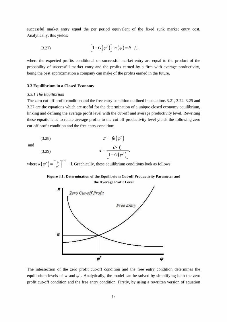
where . Graphically, these equilibrium conditions look as follows:

Figure 3.1: Determination of the Equilibrium Cut-off Productivity Parameter and

the Average Profit Level

The intersection of the zero profit cut-off condition and the free entry condition determines the

equilibrium levels of and . Analytically, the model can be solved by simplifying both the zero

profit cut-off condition and the free entry condition. Firstly, by using a rewritten version of equation

1 ,eG f

fk

.

1

ef

G

1

1k

18

3.15 to substitute for the cut-off revenue level in equation 3.21, the following transformed zero cut-off

profit condition can be derived7:

(3.30)

Secondly, using equation 3.30 to rewrite the average profit component in the free entry condition, the

free entry condition can be transformed into8:

(3.31)

Since the average productivity level depends on the cut-off productivity parameter as in equation

3.22, this model can be solved for both and . These firm-level variables are independent of the

country size L. A simplified example illustrating the derivation of the equilibrium is included in the

Appendix, Proof A10.

3.3.2 Comparative Statics Exercises

To assess the dynamics of the model in a closed economy setting, it is worth to perform some

comparative statics exercises and analytically check how the cut-off and average productivity levels

react to changes in exogenous variables. Three types of shocks can occur. Firstly, the fixed sunk

market entry costs fe can increase. In case this happens, the right-hand side of equation 3.31 increases.

To maintain balance in the rewritten free entry condition, the left-hand side in the equation needs to

increase, which requires the cut-off productivity level to decline. A lower cut-off productivity level

automatically yields a lower industry-wide average productivity level. Graphically, this shock moves

the upward-sloping free entry condition further up. Intuitively, an increase in fe makes it less attractive

for potential market entrants to enter the market, as each firm has to earn higher profits to recover the

increased fixed sunk market entry costs. Accordingly, fewer firms will enter the market, which reduces

the competitive pressure on existing firms active in the market. The existing active firms will ceteris

paribus earn higher average profits, independent of their productivity level. Thus, even initially less

productive firms are able to survive in the market, reducing the cut-off and industry-wide average

productivity levels.

Secondly, fixed production costs f can rise. In case this happens, the per period profits earned

by each firm ceteris paribus decline. This affects the zero cut-off profit condition by increasing the

productivity level necessary to earn non-negative profits, characterizing the productivity level that

makes it attractive to be active in the market. It yields a situation in which only firms with a

productivity parameter significantly higher than the initial cut-off productivity level are able to survive

in the market. Firms that can no longer cover their production costs and, thus, earn negative profits are

forced to exit the market. This selection mechanism has a positive impact on both the cut-off

productivity level and the industry-wide average productive level. Graphically, this result can be

understood by shifting the zero cut-off profit condition upward.

7 The derivation of equation 3.30 is included in the Appendix, Proof A6. 8 The derivation of equation 3.31 is included in the Appendix, Proof A7.

1

.r f

1

1 1 .eG f f

19

Thirdly, firms can be confronted with a lower death probability θ. This has exactly opposite

effects relative to an increase in the fixed sunk market entry costs. In this case, the right-hand side of

equation 3.31 declines. To maintain balance in the free entry condition, the left-hand side of the

equation needs to decrease, which requires the cut-off productivity level to increase. A higher cut-off

productivity level automatically yields a higher industry-wide average productivity level. Graphically,

this decline in the death probability moves the upward-sloping free entry condition down. Intuitively, a

lower θ makes it more attractive for potential market entrants to enter the market, as the chances of

survival in the market and earning positive profits are higher. Accordingly, more firms will enter the

market, which increases the competitive pressure on existing firms active in the market. The existing

active firms will ceteris paribus be confronted with lower market shares and lower profits. It will force

some initially active, less productive firms to exit the market, increasing the cut-off and industry-wide

average productivity levels. Only very productive firms are able to be active in the market.

3.4 Equilibrium in an Open Economy

3.4.1 Assumptions

In an open economy setting, it is assumed that n > 0 other identical countries exist, such that the world

consists of at least 2 very similar countries. Introducing trade to the model requires the inclusion three

types of export costs. Firstly, each firm exporting its product to a foreign market is confronted with

iceberg transportation costs τ, meaning that τ > 1 units of a good must be shipped in order for 1 unit to

arrive at the destination. In essence, the iceberg transportation costs cause the marginal costs of a firm

for supplying goods abroad to increase. Secondly, each firm has to pay periodic, fixed production

costs fx to produce goods for the foreign market. It is assumed that these foreign fixed production costs

are higher than the domestic fixed production costs, i.e. fx > f. Thirdly, each firm is required to pay a

fixed investment cost fex > 0 to be able to enter a foreign export market.

Defining these export costs is crucial for the development of a realistic theoretical, open

economy model. Omission would create an equilibrium outcome in which the introduction of trade in

an open economy setting has similar effects to an increase in the country size in an autarky setting. In

particular, the introduction of trade would not have effects on any of the firm level variables, including

the number of firms producing in each country, the levels of production, and the profits earned. The

existence of firm heterogeneity would not alter the impact of trade liberalization. Only consumers

would gain from the introduction of trade through the wider variety of products available in an open

economy setting.

Since the countries are identical to each other, all countries are characterized by the same

wage rate, which is still normalized to one, and country-wide aggregate variables. The profit

maximizing price for firms serving the domestic market pd(φ) is similar to one in the closed economy

setting and, hence, is equal to equation 3.11. Firms exporting goods set a profit maximizing price in

excess of the optimal domestic price, incorporating the higher marginal cost τ for serving foreign

markets. The optimal foreign price is equal to:

(3.32)

.1

x dp p

20

3.4.2 Firm Entry, Exit and Export Status

The firm entry and exit procedure described in section 3.2 remains unchanged in an open economy

setting. Prior to entering the domestic market, firms have to pay an initial fixed sunk market entry cost.

Subsequently, they discover their firm-specific productivity level and determine whether it is

profitable to start production. Firms that start production are subject to a periodic negative shock,

forcing them to exit the market immediately with probability θ.

The decision to export occurs only after firms know their productivity level and, thus, is not

subject to any export market uncertainty. Therefore, firms will only decide to export in case the profits

from serving the foreign market are non-negative. The profits earned from serving the foreign market

are equal to:

(3.33)

Using equations 3.7 and 3.32 to substitute for the revenues earned from exporting to the foreign

market, this equation can be simplified to:

(3.34)

Only firms with a productivity level high enough to earn non-negative profits from serving the foreign

market will decide to produce for the domestic market and to export. Hence, as in the closed economy

setting, it is possible to derive an adjusted zero cut-off profit condition, defining the minimum

productivity parameter φx* characterizing the firms that will be active in the foreign market. This zero

profit cut-off condition for serving the foreign market is equal to:

(3.35)

If φx* = φ

*, all firms in the industry export. In case φx

* > φ

*, there is a number of firms that solely

focuses on the domestic market. These firms, characterized by a productivity parameter φ* < φ < φx

*,

earn non-negative profits from selling their products domestically, but earn negative profits from

serving the foreign market. Firms with a productivity parameter in excess of φx* will earn profits to sell

goods both domestically and abroad.

Prior to entering the foreign market and exporting goods, firms have to assess whether it is

actually profitable to do so, given the upfront investment they have to make. As in the closed economy

setting, the dynamic process of market entry is defined by a free market entry condition. Firms will

decide to enter the foreign market in case the expected profits are sufficient to cover the per period

equivalent of the fixed sunk market entry cost. Compared to a closed economy setting, the expected

profits with trade consist of two components, namely the expected profits from serving the domestic

market and the expected profits from serving the foreign market. Again, conditional on successful

market entry, a firm’s best approximation of the future profits earned is the expected average profit

level in both the domestic and foreign market. The per period equivalent of the fixed sunk market

entry cost in the open economy setting can be derived similarly to the procedure followed in the closed

.x

x x x x x x

rp q c q f f

1 1

.F F

x x

p P If

1

1 1

.x F F

x

p P If

21

economy setting and, accordingly, is equal to equation 3.26. Then, the adjusted free entry condition in

an open economy setting is as follows:

(3.36)

where equals the average productivity parameter over all the exporting firms. Using equations 3.12

and 3.33 to substitute for the average profit levels, equation 3.36 can be simplified to:

(3.37)

3.4.3 The Link between Productivity and the Financial Performance of Firms

Before deriving, describing and discussing the open economy equilibrium, it can be proven that there

is a positive relationship between a firm’s productivity and its financial performance, supporting the

idea that financial performance is an accurate proxy for unobservable productivity in the empirical

analysis. Using equation 3.20, the sector-wide average profits earned by a firm with an average

productivity parameter, being the difference between revenues and costs, are equal to:

(3.38)

where P equals the aggregate price level in the domestic country, which in an open economy setting

depends on both the price level domestically and abroad. Foreign countries, namely, have access to

and can sell products in the domestic market. Accordingly, the foreign aggregate price level, which is

exogenous, should also be taken into account when determining the aggregate price level. Using the

inverse of equation 3.11 to substitute for the cost component in the profit function, equation 3.38 can

be rewritten as:

(3.39)

As in equations 3.16 and 3.17, the domestic aggregate sub-price index, here denoted by PD, is equal to:

(3.40)

Using the same logic, the aggregate foreign sub-price index, denoted by PF and being equal to the sum

of the individual foreign country price levels, can be expressed as follows:

(3.41)

where τ stands for the iceberg transportation costs and captures the difference between the prices

domestically and abroad. Combining equations 3.40 and 3.41 to replace for the aggregate price P,

equation 3.39 can be simplified to:

1 1 ,x x eG G f

x

1 1 .x

x x e

r rG f G f f

1

1 1,

I Ip p c

P P

1

1

11 .

Ip

P

1

1 .DP M p

1

1

1

,N

F i i

i

P M p

22

(3.42)

Assuming that in an open economy setting the domestic country trades with a sufficiently large

number of different foreign countries, the domestic aggregate price component can be removed from

equation 3.42 as it is dominated by the exogenous, aggregate foreign price level. Accordingly,

equation 3.42 can be approximated by:

(3.43)

Using equation 3.11 to substitute for the optimal average price level, equation 3.43 can further be

simplified to:

(3.44)

The first order derivative of equation 3.44 with respect to the sector-wide average productivity

parameter, which is useful to assess the link between the financial performance of firms and their

productivity level, is equal to:

(3.45)

The first order derivative of the sector-wide average profits with respect to the average productivity

parameter is strictly positive, indicating that in a setting as described above, the industry-wide average

profits earned by a firm with average efficiency react positively to a change in the average

productivity level. Intuitively, this relationship can be explained as follows. In case the sector-wide

average productivity level improves, the average profit maximizing price charged by a firm with an

average productivity level declines, as can be seen by analyzing the price specification incorporated in

equation 3.44. However, since the elasticity of substitution σ is greater than one, the decline in the

optimal price has a positive impact on the industry-wide average profit level. The combination of

higher average productivity and a lower profit maximizing price has an overall positive impact on the

sales potential of the average firm, improving the industry-wide average profitability. Hence, this

positive relationship supports the idea that the financial performance of firms can be used as an

accurate and objectively measurable proxy of productivity.

3.4.4 The Equilibrium

In equilibrium, two zero cut-off profit conditions, linking the average profits earned by firms active in

the market to the cut-off productivity level, need to hold. Firstly, as in the closed economy setting, the

1

1 1

1

.

N

i i

i

I p

M p M p

1

1

1

.

N

i i

i

I p

M p

1

1

1

1

1.

N

i i

i

I

M p

2

1

1

1 11 0.

1

N

i i

i

I

M p

23

zero cut-off profit condition determining the production status in the domestic market and derived in

equation 3.21 needs to be satisfied. Secondly, the zero cut-off profit condition determining the export

status and derived in equation 3.35 needs to hold. Analytically, the simplified, rewritten versions of

these zero profit cut-off conditions, linking the average profits earned to the cut-off productivity

parameter, look as follows9:

(3.46)

and

(3.47)

Where . Combining equations 3.46 and 3.47 yields an overall zero cut-off profit

condition characterizing the open economy setting:

(3.48)

where n stands for the total number of trading partners.

To check whether the cut-off productivity parameter defining the firms that serve both the

foreign market and the domestic market is higher than the minimum productivity parameter defining

the firms that are only active in the domestic market, it is possible to express φx* as a function of φ

*.

Namely, dividing the zero cut-off profit conditions derived in equations 3.21 and 3.35 and

incorporating the symmetry condition outlined in section 3.4.1 yields10

:

(3.49)

After substituting the optimal pricing rules derived in equations 3.11 and 3.32 for the optimal prices

charged by firms exporting goods and firms only serving the domestic market and rearranging terms,

equation 3.49 can be simplified to11

:

(3.50)

Since the assumptions are made that τ > 1 and fx > f, it can be concluded that φx* > φ

*, indicating that

not all firms export. Only the firms with a sufficiently high productivity parameter are able to produce

goods for the foreign market in a profitable way. Additionally, by carefully analyzing equation 3.50, it

can be inferred that the higher is τ or fx, the fewer firms are, apart from producing goods for the

domestic market, also serving the foreign market.

The procedure followed to determine a unique open economy equilibrium is similar to the one

followed in an autarky setting. Firstly, by using a rewritten version of equation 3.15 to substitute for

9 These simplifications are similar to the procedure followed in the closed economy setting and applied to

equation 3.28. 10

The derivation of equation 3.49 is included in the Appendix, Proof A8. 11

The derivation of equation 3.50 is included in the Appendix, Proof A8.

d fk

,x x x xf k

1

1k

1

1 .x x

p f

fp

11

.xx

f

f

, d x x x x x xp n fk p nf k

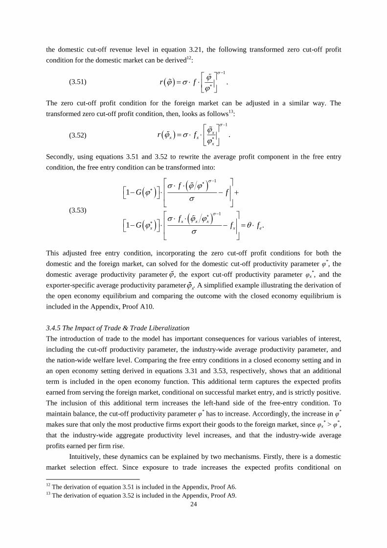
24

the domestic cut-off revenue level in equation 3.21, the following transformed zero cut-off profit

condition for the domestic market can be derived12

:

(3.51)

The zero cut-off profit condition for the foreign market can be adjusted in a similar way. The

transformed zero cut-off profit condition, then, looks as follows13

:

(3.52)

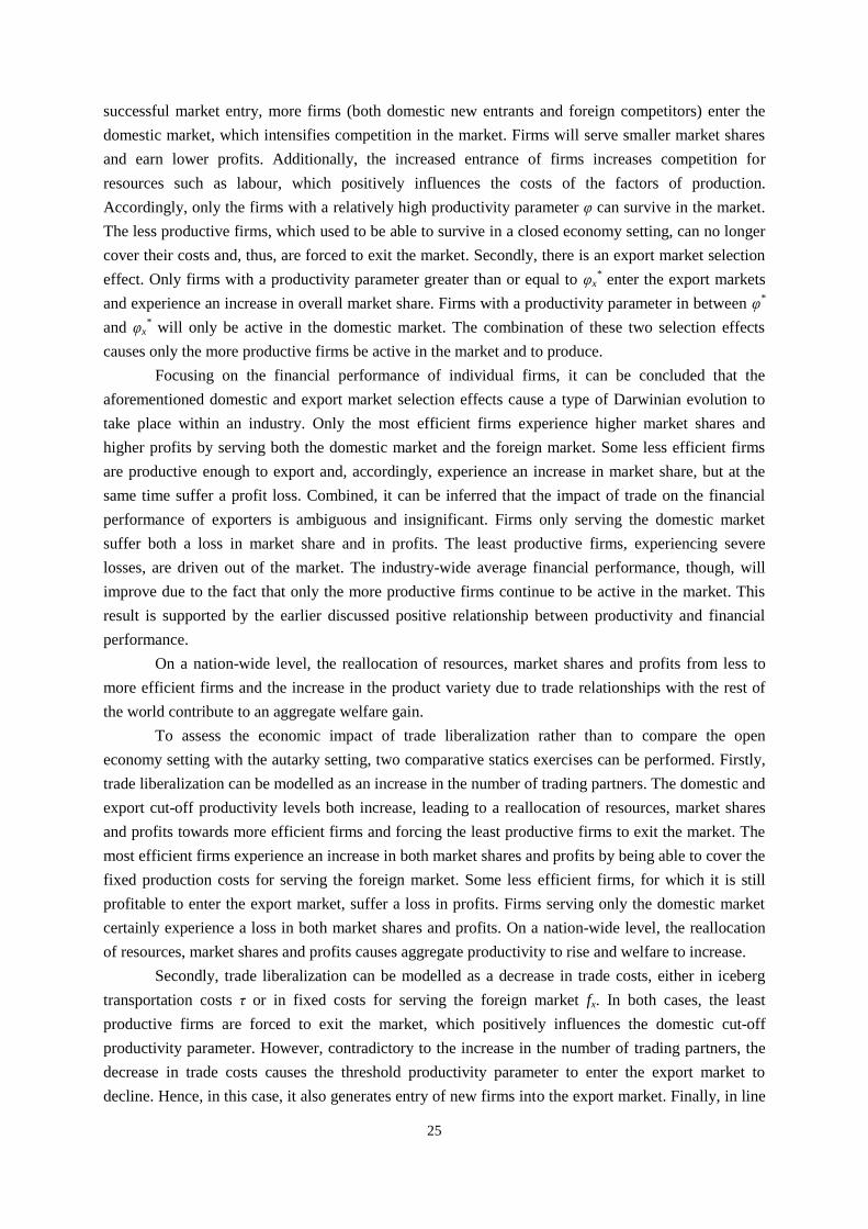
Secondly, using equations 3.51 and 3.52 to rewrite the average profit component in the free entry

condition, the free entry condition can be transformed into:

(3.53)

This adjusted free entry condition, incorporating the zero cut-off profit conditions for both the

domestic and the foreign market, can solved for the domestic cut-off productivity parameter φ*, the

domestic average productivity parameter , the export cut-off productivity parameter φx*, and the

exporter-specific average productivity parameter . A simplified example illustrating the derivation of

the open economy equilibrium and comparing the outcome with the closed economy equilibrium is

included in the Appendix, Proof A10.

3.4.5 The Impact of Trade & Trade Liberalization

The introduction of trade to the model has important consequences for various variables of interest,

including the cut-off productivity parameter, the industry-wide average productivity parameter, and

the nation-wide welfare level. Comparing the free entry conditions in a closed economy setting and in

an open economy setting derived in equations 3.31 and 3.53, respectively, shows that an additional

term is included in the open economy function. This additional term captures the expected profits

earned from serving the foreign market, conditional on successful market entry, and is strictly positive.

The inclusion of this additional term increases the left-hand side of the free-entry condition. To

maintain balance, the cut-off productivity parameter φ* has to increase. Accordingly, the increase in φ

*

makes sure that only the most productive firms export their goods to the foreign market, since φx* > φ

*,

that the industry-wide aggregate productivity level increases, and that the industry-wide average

profits earned per firm rise.

Intuitively, these dynamics can be explained by two mechanisms. Firstly, there is a domestic

market selection effect. Since exposure to trade increases the expected profits conditional on

12

The derivation of equation 3.51 is included in the Appendix, Proof A6. 13

The derivation of equation 3.52 is included in the Appendix, Proof A9.

1

.xx x

x

r f

1

1

1

1 .x x x

x x e

fG f

fG f f

x

1

.

r f

25

successful market entry, more firms (both domestic new entrants and foreign competitors) enter the

domestic market, which intensifies competition in the market. Firms will serve smaller market shares

and earn lower profits. Additionally, the increased entrance of firms increases competition for

resources such as labour, which positively influences the costs of the factors of production.

Accordingly, only the firms with a relatively high productivity parameter φ can survive in the market.

The less productive firms, which used to be able to survive in a closed economy setting, can no longer

cover their costs and, thus, are forced to exit the market. Secondly, there is an export market selection

effect. Only firms with a productivity parameter greater than or equal to φx* enter the export markets

and experience an increase in overall market share. Firms with a productivity parameter in between φ*

and φx* will only be active in the domestic market. The combination of these two selection effects

causes only the more productive firms be active in the market and to produce.

Focusing on the financial performance of individual firms, it can be concluded that the

aforementioned domestic and export market selection effects cause a type of Darwinian evolution to

take place within an industry. Only the most efficient firms experience higher market shares and

higher profits by serving both the domestic market and the foreign market. Some less efficient firms

are productive enough to export and, accordingly, experience an increase in market share, but at the

same time suffer a profit loss. Combined, it can be inferred that the impact of trade on the financial

performance of exporters is ambiguous and insignificant. Firms only serving the domestic market

suffer both a loss in market share and in profits. The least productive firms, experiencing severe

losses, are driven out of the market. The industry-wide average financial performance, though, will

improve due to the fact that only the more productive firms continue to be active in the market. This

result is supported by the earlier discussed positive relationship between productivity and financial

performance.

On a nation-wide level, the reallocation of resources, market shares and profits from less to

more efficient firms and the increase in the product variety due to trade relationships with the rest of

the world contribute to an aggregate welfare gain.

To assess the economic impact of trade liberalization rather than to compare the open

economy setting with the autarky setting, two comparative statics exercises can be performed. Firstly,

trade liberalization can be modelled as an increase in the number of trading partners. The domestic and

export cut-off productivity levels both increase, leading to a reallocation of resources, market shares

and profits towards more efficient firms and forcing the least productive firms to exit the market. The

most efficient firms experience an increase in both market shares and profits by being able to cover the

fixed production costs for serving the foreign market. Some less efficient firms, for which it is still

profitable to enter the export market, suffer a loss in profits. Firms serving only the domestic market

certainly experience a loss in both market shares and profits. On a nation-wide level, the reallocation

of resources, market shares and profits causes aggregate productivity to rise and welfare to increase.

Secondly, trade liberalization can be modelled as a decrease in trade costs, either in iceberg

transportation costs τ or in fixed costs for serving the foreign market fx. In both cases, the least

productive firms are forced to exit the market, which positively influences the domestic cut-off

productivity parameter. However, contradictory to the increase in the number of trading partners, the

decrease in trade costs causes the threshold productivity parameter to enter the export market to

decline. Hence, in this case, it also generates entry of new firms into the export market. Finally, in line

26

with the previous comparative statics exercise, trade liberalization modelled as a decrease in trade

costs generates an aggregate, nation-wide welfare gain.

3.5 Overview of the Theoretical Results

The main theoretical results based on the analysis in this section can be summarized as follows:

Trade liberalization has a positive influence on the cut-off productivity level and the industry-

wide average productivity level through processes of resource, market share and profit

reallocations. The least productive firms are forced to leave the market due to increased

competition in production factors and final goods markets. The more productive firms remain

active in the market, leading to the just mentioned higher threshold and industry-wide

productivity parameters.

Trade liberalization has a positive influence on the industry-wide average financial

performance through the aforementioned reallocation mechanisms and the direct, positive

relationship between productivity and financial performance. This theoretical result supports

the idea that financial performance is a reliable, objective and accurately measurable proxy of

productivity.

Trade liberalization has an ambiguous and insignificant impact influence on the average

productivity and financial performance of exporters. Among the group of exporters, the most

productive firms gain both in market share and profitability due to increased exposure to trade.

Some other firms, for which it is still attractive to sell goods in the foreign market, will only

experience the benefits of serving a higher market share, but suffer from a loss in profitability.

Combined, the impact of trade liberalization on the productivity and financial performance of

exporters is ambiguous and insignificant. Trade liberalization can have either a positive or a

negative impact on the threshold productivity level determining the export status of a firm,

depending on the way trade liberalization is modelled.

27

4 The Empirical Analysis

4.1 Hypotheses

The theoretical model derived and discussed in the previous section serves as a framework for

empirically analyzing the influence of trade liberalization on the industry-wide average performance

of firms due to a process of resource, market share and profit reallocations. Two central null-

hypotheses (H0) can be framed to assess the role of resource, market share and profit reallocations in

explaining the influence of trade liberalization on the industry-wide average performance of firms:

1. Trade liberalization has a positive influence on the industry-wide average performance of

firms.

2. Trade liberalization has an ambiguous and insignificant influence on the industry-wide

average performance of exporters.

The alternative hypotheses (Ha), accordingly, can be formulated as follows:

1. Trade liberalization has no influence on the industry-wide average performance of firms.

2. Trade liberalization has a significant influence on the industry-wide average performance of

exporters.

Significant evidence in favour of the two null-hypotheses supports the importance of resource, market

share and profit reallocation mechanisms, a channel which has not been analyzed intensively

empirically, in explaining how trade liberalization contributes to firm productivity and nation-wide

welfare improvements.

4.2 Data

4.2.1 Firm-Level Data & Sample

By construction, the empirical analysis requires data on the level of the firm, due to the existence of

firm heterogeneity in the total factor productivity parameter in the theoretical analysis, and over a

sufficiently long time period to facilitate the performance of a panel data analysis, the preferred

methodology. To this end, the empirical analysis employs a detailed, harmonized panel dataset with

comprehensive company-level data on the characteristics and performance of firms active in Eastern

European and Central Asian countries, gathered by the implementation of the Business Environment

and Enterprise Performance Surveys (BEEPS) and constructed by the joint effort of the World Bank

and the European Bank for Reconstruction and Development (2012).

The complete Enterprise Surveys dataset incorporates data on in total 27 countries: Albania,

Armenia, Azerbaijan, Belarus, Bosnia, Bulgaria, Croatia, Czech Republic, Estonia, the Former

Yugoslav Republic of Macedonia (FYROM), Georgia, Hungary, Kazakhstan, Kyrgyz, Latvia,

Lithuania, the Republic of Moldova, Montenegro, Poland, Romania, Russia, Serbia, Slovakia,

Slovenia, Tajikistan, Ukraine and Uzbekistan. With information collected on the basis of 150-1800

interviews per country, depending on the size of each country, and over a period of 4 years, in

particular 2002, 2005, 2007 and 200914

, the dataset constitutes a representative sample of an

economy’s private sector. In total, data on 23,570 firms has been collected.

14

The Enterprise Survey was published in 2002, 2005, 2007 and 2009, but reports information on one year

before the publishing year, i.e. 2001, 2004, 2006 and 2008.

28

The information gathered covers many different aspects of a firm, including general

information, infrastructure and services, sales and supplies, the degree of competition, capacity, land

and permits, crime, finance, business-government relations, labour, the business environment, and

performance. Relevant indicators required for the empirical analysis include total sales revenue, total

costs, the direct export intensity, firm age, foreign ownership shares, the use of foreign inputs, the

number of skilled employees, total employment, the use of foreign technologies, and 4-digit sector

affiliation (ISIC-Rev 3.1). Generally speaking, the sectors considered include both manufacturing and

services. The ISIC codes allow a more specific definition of the different sectors included in the

survey and indicate that the main activities considered are activities related to the processing of food,

textiles, garments, chemicals, plastics and rubber, non-metallic mineral products, basic metals,

fabricate metal products, machinery and equipment, electronics, other manufacturing, construction

services, other services, wholesale, retail, hotel and restaurants, transportation, and IT services. In

total, the sample includes 503 sectors, each defined by a unique 4-digit ISIC code (World Bank, 2012).

4.2.2 Sector-Level Variables

The empirical analysis extracts from the Enterprise Survey the firm-level information specified above

to construct country-specific, sector-level variables. The construction of sector-level variables is

necessary to investigate the role of resource, market share and profit reallocations in explaining the

influence of trade liberalization on the industry-wide average performance of firms. Namely, as

discussed earlier, theory suggests that trade liberalization has a positive influence on the sector-wide

cut-off productivity level and, accordingly, on the sector-wide average productivity level. To

empirically investigate this relationship, it is necessary to work with sector-wide average variables.

Hence, the unit of observation in the empirical analysis is the average firm active in an industry.

Taking the average firm as the unit of observation and analysis enables the elimination of any

structural differences in firm characteristics within a sector.

Eight country-specific, sector-level variables are constructed. Firstly, annual sector-wide

average productivity is assessed on the basis of the sector-wide average financial performance of

firms. The use of financial performance as a proxy of productivity is supported by the theoretical proof

outlined in section 3.4.3, which suggests that there is a positive relationship between productivity and

financial performance. The advantage of using financial performance instead of productivity is that

financial performance, specified in line with conventional finance literature (Berk and DeMarzo,

2007), is objectively and accurately measurable. Several researchers have attempted to accurately

measure productivity by estimating a firm’s production function. However, as discussed in section 2.2,

the estimation procedure is often problematic due to the existence of econometric selection and

simultaneity problems (Levinsohn and Petrin, 2002). In the analysis, two measures of financial

performance are constructed. The most common financial performance measure is the profit ratio.

Yearly firm-level profits are calculated by subtracting from the sales revenue the costs of labour, costs

of electricity, costs of fuel, costs of water, costs of finished goods and materials, costs of raw materials

and other intermediate goods, costs related to the purchases of fixed assets, and other costs not yet

specified. Firm-specific profit ratios are calculated by dividing the obtained profit levels by the total

annual sales revenues. The yearly sector-wide average profit over sales ratio is constructed by

averaging the firm-specific profit ratios of all firms active in a sector in a particular year, weighted by

29

each firm’s share in total sectoral employment. Employment is measured by means of the total number

of full-time workers hired by a particular firm. Using employment shares as a method for determining

weighted averages is a common procedure applied in many economic empirical studies, including

Aitken and Harrison (1999). The firm’s share in total sectoral employment, ESjct, is calculated as

follows:

(4.1)

where ESjct is the sectoral employment share characterizing sector j in country c at time t and FTEijct

stands for the number of full-time employees working at firm i active in sector j in country c at time t.

As mentioned earlier, sectors are characterized by 4-digit ISIC codes, allowing a highly specific

definition of different sectors. The annual profit over sales ratio is always in between -1 and +1. Firms

with a ratio outside this range are deleted from the dataset, as chances are high that the information

reported on these firms is subject to severe inaccuracies. Another widely used measure of financial

performance is the market share, quantifying the part of the market that is served by a firm. Since the

empirical analysis relies upon sector-wide average values, annual sector-wide average market shares

are constructed by determining the yearly sector-wide average sales revenues, and dividing these

revenue levels by the annual country-wide average sales. Again, sectors are characterized by 4-digit

ISIC codes, allowing a highly specific definition of different sectors. The calculated annual sector-

wide average market shares are by definition in between 0 and +1.

Secondly, yearly sector-wide export intensities are used to model the process of trade

liberalization and, thus, represent a crucial sector-level variable in the model. An increase in the

sector-wide export intensity over the period 2002-2009 is a clear indication of an economy opening up

to trade, with sectors trying to exploit the increased sales potential by selling products in foreign

markets. The yearly sector-wide export intensities are determined with the help of the survey

information on firm-specific direct export intensities. The assumption that the survey information on

export intensities is a representative basis for calculating sector-wide export intensities is supported by

a simple comparison exercise. Comparing the sector-wide export shares, calculated by dividing the

sector-wide export values by the country-wide export values, determined for a random subsample of

2-digit ISIC code specified sectors and countries in the Enterprise Survey with the official country-

specific export shares of the corresponding 2-digit HTS code specified sectors reported by the

International Trade Centre provides sufficient evidence for assuming that the Enterprise Survey is a

representative basis for estimating sector-wide export intensities. The Enterprise Survey defines the

firm-specific direct export intensity as the total value of goods directly exported to foreign markets as

a percentage of overall sales. The direct export intensities are used to determine the total annual firm-

specific export values. Using the 4-digit ISIC code sector definition, the firm-specific export values

are used as inputs to calculate the annual sector-wide export values. By dividing these export values

by the yearly nation-wide sales values, being the sum of the sector-wide sales values in a particular

year, the annual sector-wide average export intensities can be determined. By definition, the yearly

sector-wide export intensities are in between 0 and +1, with a value of +1 indicating that 100% of a

sector’s sales are exported to foreign markets.

,

ijct

jct

ijct

i

FTEES

FTE

30

Thirdly, the natural logarithm of the average age of firms active in 4-digit ISIC code specified

sectors is determined to control for structural differences between firms and industries that can

possibly bias the relationship between trade liberalization and performance. It may be argued that

more mature firms have established a dominant position in the market, are producing a unique product

and are using production, marketing and sales strategies that have proven to be efficient. These firms

may perform structurally better compared to less mature firms. Since the empirical analysis uses the

average firm active in a sector as the unit of observation, sector-wide average ages are used rather than

the firm-specific ages. The Enterprise Survey reports information on the year that a firm started its

operations, which can be used to calculate the firm-specific age. By taking the difference between the

survey year15

and the year a firm started its operations, the firm-specific age can be determined.

Accordingly, as in the case of the sector-wide profit ratio, the yearly sector-wide average age of firms

is constructed by averaging the firm-specific ages of all firms active in a 4-digit ISIC code defined

sector in a particular year, weighted by each firm’s share in total sectoral employment. Employment

shares are calculated as defined in equation 4.1.

Fourthly, since firm size might be a firm-specific characteristic that has a structural impact on

the financial performance, the natural logarithm of the average size of firms active in 4-digit ISIC code

defined sectors is calculated and included in the empirical analysis. In particular, it may be argued that

smaller firms are more flexible and have greater potential to grow, which allows them to fully benefit

from trade liberalization via entering new markets. In case this is true, firm size may have a

structurally positive impact on the performance of smaller companies in an open economy setting,

which can bias the empirical link between trade liberalization and performance. Firm size is assessed

on the basis of the total number of full-time employees hired by a company. A full-time employee is

defined as a worker who is contracted for a term of one or more fiscal years, who has a guaranteed

renewal of his or her employment contract and who works 8 or more hours per day (World Bank,

2012). As in the case of the sector-wide profit ratio and the average age, the sector-wide average firm

size is determined by averaging the firm-specific sizes of all firms active in a particular sector in a

specific year, weighted by each firm’s share in total sectoral employment. Employment shares are

calculated as defined in equation 4.1.

Fifthly, the share of foreign ownership, measured according to a sector-wide average

percentage, is determined. The reason for calculating this variable is that many researchers have

shown that there is a statistically significant and positive relationship between foreign direct

investments, which are often proxied by the share of foreign ownership, and the performance of firms

in emerging markets. In particular, Aitken and Harrison (1999) show that production plants clearly

benefit from the productive advantages of foreign owners through a process of technology diffusion

and learning effects, using a sample of Venezuelan firms. Therefore, firms and sectors receiving

significant amounts of foreign direct investments may structurally perform better, which can possibly

bias the relationship between trade liberalization and performance. Sector-wide average shares of

foreign ownership rather than firm-specific foreign ownership stakes are used since the empirical

analysis uses the average firm active in a sector as the unit of observation. The Enterprise Survey

provides information on the percentage of the firm that is owned by private foreign individuals,

15 The Enterprise Survey was published in 2002, 2005, 2007 and 2009, but reports information on one year

before the publishing year, i.e. 2001, 2004, 2006 and 2008.

31

companies or organisations. The yearly sector-wide average shares of foreign ownership are

constructed by averaging the firm-specific foreign ownership stakes of all firms active in a 4-digit

ISIC code defined sector in a particular year, weighted by each firm’s share in total sectoral

employment. Employment shares are calculated as defined in equation 4.1. By definition, the yearly

sector-wide average shares of foreign ownership are in between 0 and +1. A value of +1 indicates that,

on average, the companies active in a particular sector are completely owned by private foreign

individuals, companies or organisations.

Sixthly, the sector-wide average skill intensity is determined with the help of the information

on the number of skilled workers employed by a firm. Skill intensity is a relevant variable to include

as a control variable in the empirical analysis since factor market competition is an important feature

influencing a company’s ability to survive in an open economy market. Firms with good financial

performance can attract more skilled and talented workers, resulting in a relatively higher proportion

of skilled workers employed and having a positive influence on productivity and performance.

However, hiring more skilled workers also comes at the cost of paying higher wages. The Enterprise

Survey reports information on each firm’s number of skilled workers hired. Skilled workers are

defined as ‘workers engaged in fabricating, processing, assembling, inspecting, receiving, storing,

handling, packing, warehousing, shipping, maintenance, repair, product development, auxiliary

production for the plant’s own use, recordkeeping, and other services closely associated with these

production operations’. Workers with functions above the supervisory level are excluded from this

definition. Skilled workers are also workers that have some special knowledge or skill in their work. In

terms of education, a skilled worker attended a college, university or technical school (World Bank,

2012). Dividing the number of skilled workers by the total number of full-time workers employed by a

firm yields a firm-specific measure of skill intensity. This skill intensity measure is a ratio on the

interval [0, 1]. The closer is the ratio to 1, the higher is the proportion of skilled workers within the

complete firm-specific workforce. The yearly sector-wide average skill intensities are calculated by

averaging the firm-specific skill intensities of all firms active in a 4-digit ISIC code specified sector in

a particular year, weighted by each firm’s share in total sectoral employment. Employment shares are

calculated as defined in equation 4.1.

Seventhly, related to the share of foreign ownership, sector-wide average foreign technology

dummies are calculated. The idea behind inclusion of a foreign technology variable is essentially

similar to the one behind the inclusion of the earlier described foreign ownership variable. Again, the

use of sophisticated foreign technologies may have a positive influence on a firm’s performance.

Additionally, a process of technology diffusion and learning effects may boost technological

development in the foreign direct investment receiving country, enhancing economic growth and,

accordingly, also allowing firms that do not use foreign technologies to benefit. The Enterprise Survey

provides firm-specific foreign technology dummies, with a value 0 referring to firms not using any

foreign technologies and a value 1 defining firms that have implemented foreign technologies in their

production processes. Firm-specific dummies are converted into sector-wide average foreign

technology dummies by averaging the firm-specific foreign technology dummies of all firms active in

a 4-digit ISIC code specified sector in a particular year, weighted by each firm’s share in total sectoral

employment. Again, employment shares are calculated as defined in equation 4.1.

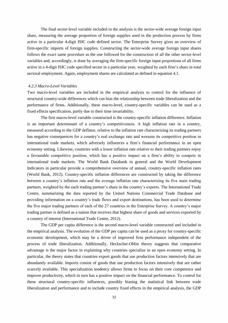
32

The final sector-level variable included in the analysis is the sector-wide average foreign input

share, measuring the average proportion of foreign supplies used in the production process by firms

active in a particular 4-digit ISIC code defined sector. The Enterprise Survey gives an overview of

firm-specific imports of foreign supplies. Constructing the sector-wide average foreign input shares

follows the exact same procedure as the one followed for the construction of all the other sector-level

variables and, accordingly, is done by averaging the firm-specific foreign input proportions of all firms

active in a 4-digit ISIC code specified sector in a particular year, weighted by each firm’s share in total

sectoral employment. Again, employment shares are calculated as defined in equation 4.1.

4.2.3 Macro-Level Variables

Two macro-level variables are included in the empirical analysis to control for the influence of

structural country-wide differences which can bias the relationship between trade liberalization and the

performance of firms. Additionally, these macro-level, country-specific variables can be used as a

fixed effects specification, partly due to their time invariability.

The first macro-level variable constructed is the country-specific inflation difference. Inflation

is an important determinant of a country’s competitiveness. A high inflation rate in a country,

measured according to the GDP deflator, relative to the inflation rate characterizing its trading partners

has negative consequences for a country’s real exchange rate and worsens its competitive position in

international trade markets, which adversely influences a firm’s financial performance in an open

economy setting. Likewise, countries with a lower inflation rate relative to their trading partners enjoy

a favourable competitive position, which has a positive impact on a firm’s ability to compete in

international trade markets. The World Bank Databank in general and the World Development

Indicators in particular provide a comprehensive overview of annual, country-specific inflation rates

(World Bank, 2012). Country-specific inflation differences are constructed by taking the difference

between a country’s inflation rate and the average inflation rate characterizing its five main trading

partners, weighted by the each trading partner’s share in the country’s exports. The International Trade

Centre, summarizing the data reported by the United Nations Commercial Trade Database and

providing information on a country’s trade flows and export destinations, has been used to determine

the five major trading partners of each of the 27 countries in the Enterprise Survey. A country’s major

trading partner is defined as a nation that receives that highest share of goods and services exported by

a country of interest (International Trade Centre, 2012).

The GDP per capita difference is the second macro-level variable constructed and included in

the empirical analysis. The evolution of the GDP per capita can be used as a proxy for country-specific

economic development, which may be a driver of improved firm performance independent of the

process of trade liberalization. Additionally, Heckscher-Ohlin theory suggests that comparative

advantage is the major factor in explaining why countries specialize in an open economy setting. In

particular, the theory states that countries export goods that use production factors intensively that are

abundantly available. Imports consist of goods that use production factors intensively that are rather

scarcely available. This specialization tendency allows firms to focus on their core competence and

improve productivity, which in turn has a positive impact on the financial performance. To control for

these structural country-specific influences, possibly biasing the statistical link between trade

liberalization and performance and to include country fixed effects in the empirical analysis, the GDP

33

per capita difference is constructed. The World Bank Databank in general and the World Development

Indicators in particular provide all the necessary information for calculating this macro-level variable

(World Bank, 2012). To eliminate the influence of price changes, the GDP per capita is measured in

US Dollars specific for the year 2000. Again, as in the case of the inflation difference, the GDP per

capita difference is constructed by subtracting from the GDP per capita a country in the Enterprise

Survey sample the average GDP per capita characterizing its five main trading partners, weighted by

the each trading partner’s share in the country’s exports. The five major trading partners are

determined on the basis of the export values and destination data provided by the International Trade

Centre (2012).

4.2.4 Descriptive Statistics

The data obtained and described are characterized by some interesting descriptive features. Table 4.1

presents a comprehensive overview of the descriptive statistics of the overall sample, providing

information on sector-wide sales, profits, aggregate financial performance, export intensities, shares of

foreign ownership, the use of foreign technologies, the use of foreign supplies, firm size, firm age, the

number of full-time workers employed and the two macro-level variables.

The average sales value for all countries considered, after deleting sales values that give rise to

profit ratios smaller than -1 or greater than +1, is approximately equal to $4.6 billion, with a maximum

of $100 trillion for a firm in Uzbekistan. The average profits earned, only taking into account profits

that produce reasonable profit ratios, are equal to $3.7 billion.

The mean of the sector-wide average profit ratio, a variable which is highly relevant for the

empirical analysis, is 0.410. The corresponding standard deviation of 0.335 indicates that there is quite

some dispersion among sectors and firms in terms of their financial performance. Out of the sample of

27 countries, fifteen countries are characterized by a higher profit ratio. These countries include

Belarus, Bosnia, Bulgaria, Croatia, Czech Republic, Estonia, Kyrgyz, Latvia, Lithuania, Romania,

Russia, Slovakia, Slovenia, Ukraine and Uzbekistan. The lowest aggregate profit ratio, equal to the

earlier defined lower bound of -1, is characterizing Azerbaijan, the Former Yugoslav Republic of

Macedonia, Lithuania and Russia.

Sector-wide exports vary widely among different industries. The mean of the sector-wide

average exports equals $429 million with a standard deviation of $43.8 billion. Again, sectors and

countries differ considerably in terms of average export values. The country with the largest sector-

wide exports is Uzbekistan, with an average industry-wide export value of $13.4 billion. Looking at

the sector-wide export intensity, the overall sample is characterized by an average export intensity of

0.124. Only sector-wide export intensities in between 0 and +1 are taken into account. Countries with

a higher sector-wide export intensity are Albania, Bosnia, Bulgaria, Croatia, Czech Republic, Estonia,

Hungary, Latvia, Lithuania, Moldova, Romania, Slovakia, Slovenia and Ukraine. The most open

economies are Bulgaria and Slovenia, with average sector-wide export intensities of 0.221 and 0.227,

respectively. Graph 4.1 on page 35 plots the development of the sector-wide average profit ratio and

the sector-wide average export intensity for the overall sample over the period 2002-2009.

Graph 4.1 shows that the sector-wide average profit ratio and the sector-wide average export

intensity follow a very similar trend, which possibly indicates a positive relationship between the

sector-wide export intensity and the aggregate financial performance. Both the profit ratio and the

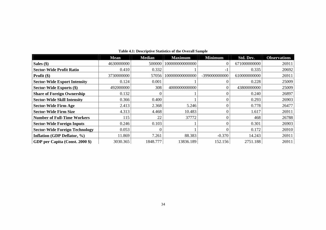
34

Table 4.1: Descriptive Statistics of the Overall Sample

Kolom1 Mean Median Maximum Minimum Std. Dev. Observations

Sales ($) 4630000000 500000 100000000000000 0 671000000000 26911

Sector-Wide Profit Ratio 0.410 0.332 1 -1 0.335 20692

Profit ($) 3730000000 57056 100000000000000 -399000000000 610000000000 26911

Sector-Wide Export Intensity 0.124 0.001 1 0 0.228 25009

Sector-Wide Exports ($) 492000000 308 4000000000000 0 43800000000 25009

Share of Foreign Ownership 0.132 0 1 0 0.240 26897

Sector-Wide Skill Intensity 0.366 0.400 1 0 0.293 26903

Sector-Wide Firm Age 2.413 2.368 5.246 0 0.778 26477

Sector-Wide Firm Size 4.313 4.468 10.483 0 1.617 26911

Number of Full-Time Workers 115 22 37772 0 468 26788

Sector-Wide Foreign Inputs 0.246 0.103 1 0 0.301 26903

Sector-Wide Foreign Technology 0.053 0 1 0 0.172 26910

Inflation (GDP Deflator, %) 11.869 7.261 88.383 -0.370 14.243 26911

GDP per Capita (Const. 2000 $) 3030.365 1848.777 13836.189 152.156 2751.188 26911

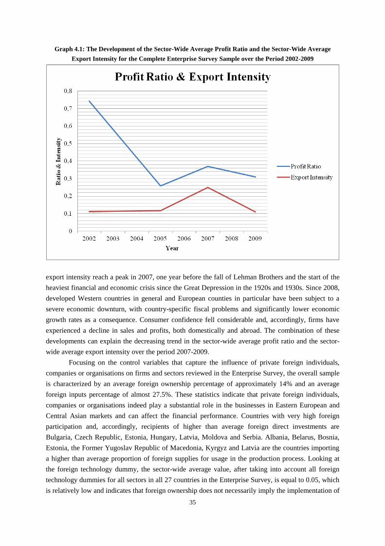
35

Graph 4.1: The Development of the Sector-Wide Average Profit Ratio and the Sector-Wide Average

Export Intensity for the Complete Enterprise Survey Sample over the Period 2002-2009

export intensity reach a peak in 2007, one year before the fall of Lehman Brothers and the start of the

heaviest financial and economic crisis since the Great Depression in the 1920s and 1930s. Since 2008,

developed Western countries in general and European counties in particular have been subject to a

severe economic downturn, with country-specific fiscal problems and significantly lower economic

growth rates as a consequence. Consumer confidence fell considerable and, accordingly, firms have

experienced a decline in sales and profits, both domestically and abroad. The combination of these

developments can explain the decreasing trend in the sector-wide average profit ratio and the sector-

wide average export intensity over the period 2007-2009.

Focusing on the control variables that capture the influence of private foreign individuals,

companies or organisations on firms and sectors reviewed in the Enterprise Survey, the overall sample

is characterized by an average foreign ownership percentage of approximately 14% and an average

foreign inputs percentage of almost 27.5%. These statistics indicate that private foreign individuals,

companies or organisations indeed play a substantial role in the businesses in Eastern European and

Central Asian markets and can affect the financial performance. Countries with very high foreign

participation and, accordingly, recipients of higher than average foreign direct investments are

Bulgaria, Czech Republic, Estonia, Hungary, Latvia, Moldova and Serbia. Albania, Belarus, Bosnia,

Estonia, the Former Yugoslav Republic of Macedonia, Kyrgyz and Latvia are the countries importing

a higher than average proportion of foreign supplies for usage in the production process. Looking at

the foreign technology dummy, the sector-wide average value, after taking into account all foreign

technology dummies for all sectors in all 27 countries in the Enterprise Survey, is equal to 0.05, which

is relatively low and indicates that foreign ownership does not necessarily imply the implementation of

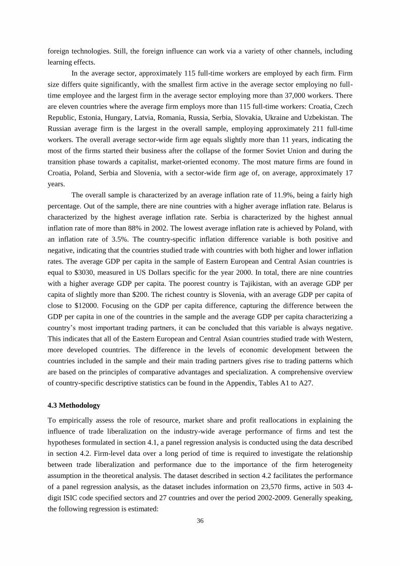
36

foreign technologies. Still, the foreign influence can work via a variety of other channels, including

learning effects.

In the average sector, approximately 115 full-time workers are employed by each firm. Firm

size differs quite significantly, with the smallest firm active in the average sector employing no full-

time employee and the largest firm in the average sector employing more than 37,000 workers. There

are eleven countries where the average firm employs more than 115 full-time workers: Croatia, Czech

Republic, Estonia, Hungary, Latvia, Romania, Russia, Serbia, Slovakia, Ukraine and Uzbekistan. The

Russian average firm is the largest in the overall sample, employing approximately 211 full-time

workers. The overall average sector-wide firm age equals slightly more than 11 years, indicating the

most of the firms started their business after the collapse of the former Soviet Union and during the

transition phase towards a capitalist, market-oriented economy. The most mature firms are found in

Croatia, Poland, Serbia and Slovenia, with a sector-wide firm age of, on average, approximately 17

years.

The overall sample is characterized by an average inflation rate of 11.9%, being a fairly high

percentage. Out of the sample, there are nine countries with a higher average inflation rate. Belarus is

characterized by the highest average inflation rate. Serbia is characterized by the highest annual

inflation rate of more than 88% in 2002. The lowest average inflation rate is achieved by Poland, with

an inflation rate of 3.5%. The country-specific inflation difference variable is both positive and

negative, indicating that the countries studied trade with countries with both higher and lower inflation

rates. The average GDP per capita in the sample of Eastern European and Central Asian countries is

equal to $3030, measured in US Dollars specific for the year 2000. In total, there are nine countries

with a higher average GDP per capita. The poorest country is Tajikistan, with an average GDP per

capita of slightly more than $200. The richest country is Slovenia, with an average GDP per capita of

close to $12000. Focusing on the GDP per capita difference, capturing the difference between the

GDP per capita in one of the countries in the sample and the average GDP per capita characterizing a

country’s most important trading partners, it can be concluded that this variable is always negative.

This indicates that all of the Eastern European and Central Asian countries studied trade with Western,

more developed countries. The difference in the levels of economic development between the

countries included in the sample and their main trading partners gives rise to trading patterns which

are based on the principles of comparative advantages and specialization. A comprehensive overview

of country-specific descriptive statistics can be found in the Appendix, Tables A1 to A27.

4.3 Methodology

To empirically assess the role of resource, market share and profit reallocations in explaining the

influence of trade liberalization on the industry-wide average performance of firms and test the

hypotheses formulated in section 4.1, a panel regression analysis is conducted using the data described

in section 4.2. Firm-level data over a long period of time is required to investigate the relationship

between trade liberalization and performance due to the importance of the firm heterogeneity

assumption in the theoretical analysis. The dataset described in section 4.2 facilitates the performance

of a panel regression analysis, as the dataset includes information on 23,570 firms, active in 503 4-

digit ISIC code specified sectors and 27 countries and over the period 2002-2009. Generally speaking,

the following regression is estimated:

37

(4.2)

where FPijt is the average financial performance of firms active in sector i in country j at time t, Expijt

is the sector-wide export intensity for sector i in country j at time t, and x’ijt is a vector of control

variables, including the sector-wide average firm age, the sector-wide average firm size, the sector-

wide average skill intensity, the sector-wide average foreign ownership share, sector-wide foreign

technology dummies, and the sector-wide average foreign input share. A significant and positive

coefficient β1 supports the hypothesis that trade liberalization has a positive impact on the performance

of firms through a process of resource, market share and profit reallocations from less to more

productive firms. An important assumption underlying the empirical analysis of equation 4.2 is the

independence of the sector-specific intercepts, the country-specific intercepts, the time-specific

intercepts and the sector-, country- and time-specific error term, resulting from the estimation. To

account for this, it is essential to model different sector-specific, country-specific and time-specific

intercepts rather than a general constant. Econometrically, this can be achieved via the fixed effects

estimation procedure (Verbeek, 2008). δi, δj and δt are dummies for the different 4-digit ISIC code

specified sectors, the 27 Eastern European and Central Asian countries studied and the 4 years

considered and are used to apply the fixed effects specification. Firm fixed effects are not necessary,

since all structural differences between firms are eliminated by taking the average firm as the unit of

observation and analysis.

Five different empirical specifications of the model outlined in equation 4.2 are estimated to

investigate the empirical link between trade liberalization and performance and to test the hypotheses

formulated in section 4.1. Firstly, a model is constructed that regresses the sector-wide average profit

ratio on the sector-wide export intensity, the sector-wide average firm age, the sector-wide average

firm size, the sector-wide average skill intensity, the sector-wide average foreign ownership share, the

sector-wide foreign technology dummies, and the sector-wide average foreign input share. Formally,

this regression model looks as follows:

(4.3)

where PRijt is the average profit ratio of firms active in sector i in country j at time t, Expijt is the

sector-wide export intensity for sector i in country j at time t, and x’ijt is a vector of control variables,

including the control variables specified above and related to firm age, size, foreign participation and

influence and skill intensity. The model is estimated using sector, country and time fixed effects by

including the industry-specific, country-specific and time-specific dummies δi, δj and δt.

Secondly, a model is estimated using a different fixed effects specification. This model serves

as a robustness check to the first model. Instead of including the country-specific dummies δj, country

fixed effects are applied by incorporating the two macro-level variables described in section 4.2.3,

namely the inflation difference and the GDP per capita difference, into the empirical model. Since the

inflation difference and GDP per capita difference are largely time invariant and country-specific,

these two variables can be used as alternatives for the conventional country dummies. Sector and time

fixed effects are captured by the conventional sector-specific and time-specific dummies δi and δt.

Formally, this regression model looks as follows:

'

1 , ijt ijt ijt i j t ijtFP Exp x

'

1 , ijt ijt ijt i j t ijtPR Exp x

38

(4.4)

where PRijt is the average profit ratio of firms active in sector i in country j at time t, Expijt is the

sector-wide export intensity for sector i in country j at time t, x’ijt is a vector of control variables,

including the control variables related to firm age, size, foreign participation and influence and skill

intensity, ΔInflationjt is the inflation difference between country j and five of its main trading partners

at time t, and ΔGDPpcjt is the GDP per capita difference between country j and five of its main trading

partners at time t. δi and δt are sector-specific and time-specific dummies, capturing sector and time

fixed effects.

Thirdly, a model in first differences is estimated. Estimating this model eliminates sector and

country fixed effects, though still incorporates time fixed effects and allows the inclusion of the

country-specific inflation difference and the GDP per capita difference as separate explanatory

variables. Again, this model specification serves as a robustness check to the first model. Formally,

this model looks as follows:

(4.5)

where ΔPRijt is the difference between the average profit ratio of firms active in sector i in country j at

time t and time t-1, ΔExpijt is the change in the sector-wide export intensity for sector i in country j

from time t-1 to time t, and Δx’ijt is a vector of control variables, specified in first differences and

including the control variables related to firm age, size, foreign participation and influence and skill

intensity. Δ(ΔInflationjt) is the change in the inflation difference between country j and five of its main

trading partners from time t-1 to time t, and Δ(ΔGDPpcjt) is the change in the GDP per capita

difference between country j and five of its main trading partners from time t-1 to time t. δt is a time-

specific dummy, capturing the time fixed effects. Due to the estimation in first differences, fewer

observations are taken into account in the empirical analysis. Instead of four, only three time periods

can be considered, namely the period 2002-2005, 2005-2007 and 2007-2009.

Fourthly, a model using the sector-wide average market share as the dependent variable is

estimated. As described in section 4.2.2, the sector-wide average market share is a widely-used

alternative for the profit ratio as a proxy of financial performance (Berk and DeMarzo, 2007) and

quantifies the part of the market that is served by an average firm active in a 4-digit ISIC code

specified sector. The use of an alternative dependent variable allows checking the stability and the

robustness of the results produced by the first two model specifications. The independent and

explanatory variables are similar to the ones employed in these two regression models. Formally, this

model is specified as follows:

(4.6)

where MSijt is the average market share of firms active in sector i in country j at time t, Expijt is the

sector-wide export intensity for sector i in country j at time t, and x’ijt is a vector of control variables,

including the control variables specified earlier and related to firm age, size, foreign participation and

influence and skill intensity. The model is estimated using sector, country and time fixed effects by

'

1 1 2 , ijt ijt ijt jt jt i t ijtPR Exp x Inflation GDPpc

'

1 1 2 , ijt ijt ijt jt jt t ijtPR Exp x Inflation GDPpc

'

1 , ijt ijt ijt i j t ijtMS Exp x

39

including the industry-specific, country-specific and time-specific dummies δi, δj and δt. The country-

specific macro-level variables are not included.

Fifthly, a model is estimated using a subsample of only exporting firms. Exporters are defined

as firms with strictly positive direct export intensities. Using the subsample of only exporters allows

testing the hypothesis that trade liberalization has an ambiguous and insignificant impact on the

aggregate performance of exporters. Supporting this hypothesis provides additional evidence for the

importance of resource, market share and profit reallocations from less to more productive firms in

explaining the relationship between trade liberalization and the sector-wide average performance. In

this model, the sector-wide average profit ratio is again used as a proxy for performance and as the

dependent variable. The independent variables are similar to the ones used in the first, the second and

the fourth model specification. Formally, this model is specified as follows:

(4.7)

where PRijt is the average profit ratio of exporting firms active in sector i in country j at time t, Expijt is

the sector-wide export intensity for sector i in country j at time t, and x’ijt is a vector of control

variables, including the control variables specified earlier and related to the exporter’s age, size,

foreign participation and influence and skill intensity. The model is estimated using sector, country

and time fixed effects by including the industry-specific, country-specific and time-specific dummies

δi, δj and δt. An insignificant coefficient β1 supports the hypothesis that trade liberalization has an

ambiguous and insignificant impact on the performance of exporters.

4.4 Empirical Results

4.4.1 Regression Results for the Sector-Wide Profit Ratio

The panel regressions as outlined in the previous section yield some very interesting results regarding

the role of resource, market share and profit reallocations in explaining the influence of trade

liberalization on the industry-wide average performance of firms. The results of the first regression

model explaining the sector-wide average profit ratio by means of the sector-wide average export

intensity and a group of control variables and applying sector-specific, country-specific and time-

specific dummies to capture sector, country and time fixed effects are summarized in Table 4.2.

By studying the reported results, it can be concluded that the sector-wide export intensity has a

significantly positive impact on the sector-wide average profit ratio, using both a 5% and a 10%

significance level and independent of the type of control variables included. The regression excluding

all control variables shows a positive relationship between the sector-wide export intensity and the

sector-wide average profit ratio at a 5% significance level. The models including control variables

related to the sector-wide average firm age, the sector-wide average firm size, the sector-wide average

skill intensity, the sector-wide average shares of foreign ownership, the sector-wide average foreign

technology variable and the sector-wide average foreign input shares reveal a positive impact of the

sector-wide export intensity on the sector-wide average profit ratio at a 5% significance level. The

most extensive model, including all control variables and being characterized by a high R2 statistic of

0.47, shows the most significant positive impact of the sector-wide export intensity on the sector-wide

'

1 , ijt ijt ijt i j t ijtPR Exp x

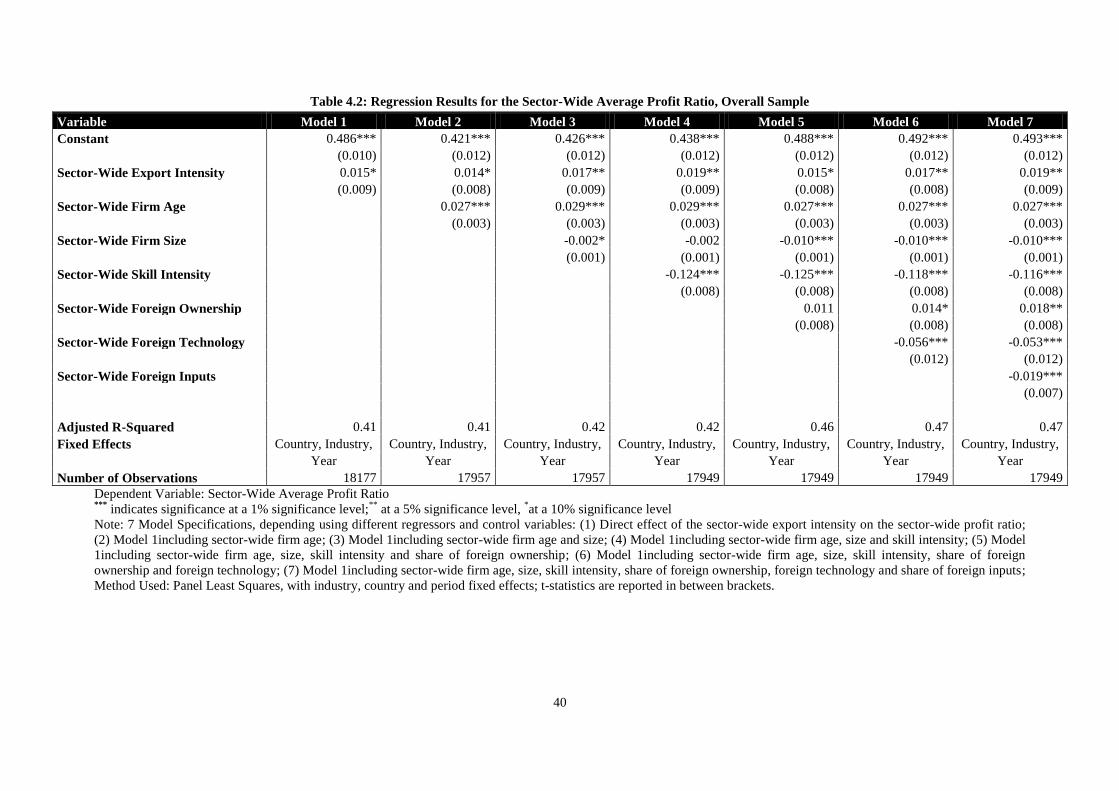
40

Table 4.2: Regression Results for the Sector-Wide Average Profit Ratio, Overall Sample

Dependent Variable: Sector-Wide Average Profit Ratio ***

indicates significance at a 1% significance level;**

at a 5% significance level, *at a 10% significance level

Note: 7 Model Specifications, depending using different regressors and control variables: (1) Direct effect of the sector-wide export intensity on the sector-wide profit ratio;

(2) Model 1including sector-wide firm age; (3) Model 1including sector-wide firm age and size; (4) Model 1including sector-wide firm age, size and skill intensity; (5) Model

1including sector-wide firm age, size, skill intensity and share of foreign ownership; (6) Model 1including sector-wide firm age, size, skill intensity, share of foreign

ownership and foreign technology; (7) Model 1including sector-wide firm age, size, skill intensity, share of foreign ownership, foreign technology and share of foreign inputs;

Method Used: Panel Least Squares, with industry, country and period fixed effects; t-statistics are reported in between brackets.

Variable Model 1 Model 2 Model 3 Model 4 Model 5 Model 6 Model 7

Constant 0.486*** 0.421*** 0.426*** 0.438*** 0.488*** 0.492*** 0.493***

(0.010) (0.012) (0.012) (0.012) (0.012) (0.012) (0.012)

Sector-Wide Export Intensity 0.015* 0.014* 0.017** 0.019** 0.015* 0.017** 0.019**

(0.009) (0.008) (0.009) (0.009) (0.008) (0.008) (0.009)

Sector-Wide Firm Age 0.027*** 0.029*** 0.029*** 0.027*** 0.027*** 0.027***

(0.003) (0.003) (0.003) (0.003) (0.003) (0.003)

Sector-Wide Firm Size -0.002* -0.002 -0.010*** -0.010*** -0.010***

(0.001) (0.001) (0.001) (0.001) (0.001)

Sector-Wide Skill Intensity -0.124*** -0.125*** -0.118*** -0.116***

(0.008) (0.008) (0.008) (0.008)

Sector-Wide Foreign Ownership 0.011 0.014* 0.018**

(0.008) (0.008) (0.008)

Sector-Wide Foreign Technology -0.056*** -0.053***

(0.012) (0.012)

Sector-Wide Foreign Inputs -0.019***

(0.007)

Adjusted R-Squared 0.41 0.41 0.42 0.42 0.46 0.47 0.47

Fixed Effects Country, Industry, Country, Industry, Country, Industry, Country, Industry, Country, Industry, Country, Industry, Country, Industry,

Year Year Year Year Year Year Year

Number of Observations 18177 17957 17957 17949 17949 17949 17949

41

average profit ratio. By calculating the point elasticity16

, using the coefficient of 0.019 for the

aggregate export intensity in the most extensive model and the means of the sector-wide profit ratio

and the sector-wide export intensity for the overall sample, it can be inferred that an increase in the

aggregate export intensity of 1% gives rise to a significant improvement in the aggregate financial

performance of firms of 0.006%.

These results indicate that trade liberalization has a positive impact on the sector-wide

financial performance of firms and, since the financial performance is used as a proxy for productivity,

on the sector-wide productivity level. This positive relationship proves that resource, market share and

profit reallocations from less to more productive firms play an important role in open economies and

may serve as drivers of productivity and nation-wide aggregate welfare improvements. The positive

impact of trade liberalization on the sector-wide average performance suggests that increasing trade

relationships and exports alter firm entry and exit dynamics, force the least productive firms to leave

the market due to increasing competition in both factor and final goods markets, give rise to a pool of

highly productive firms surviving and active in the market and produce aggregate efficiency

improvements. Overall, the results provide significant and robust evidence not to reject the first null-

hypothesis related to the complete sample and formulated in section 4.117

.

The results in Table 4.2 indicate that the natural logarithm of the sector-wide average firm age

has a robust and positive impact on the sector-wide financial performance of firms, significant at a 1%

significance level and independent of the exact model specification. The high significance of this

variable indicates that the sector-wide average firm age is an important control variable to be included

in the model. However, inclusion of the natural logarithm of the sector-wide average firm age has no

immediate effect on the explanatory power of the model, as the adjusted R2 statistic does not change

and still is equal to 0.41. The empirical outcome suggests that sectors with on average more mature

firms tend to perform better. Firms that have on average been in operations for a longer period of time

may have gained the expertise to produce and sell their products in an efficient and, accordingly, more

profitable way. These kinds of firms may rely upon production techniques, distribution networks and

marketing strategies that have proven to work in the past. Less mature firms may still be in a process

of development, which comes at the cost of efficiency and productivity. This outcome is in line with

the conclusions drawn by Hannan and Freeman (1984). They suggest that older firms tend to make use

of more efficient techniques, which allows them to make a reliable and accountable impression on

customers and, accordingly, to perform better.

The empirical results regarding the natural logarithm of the sector-wide average firm size are

not as robust as the results regarding the natural logarithm of the sector-wide average firm age. The

model including both the sector-wide firm age and the sector-wide firm size as the only control

variables shows a negative impact of firm size on average performance, significant at a 10%

significance level. The model that also includes sector-wide skill intensity as a control variable

indicates an insignificant relationship between aggregate firm size and the sector-wide average

financial performance. More extensive models, including control variables related to foreign

participation, produce more stable and robust results, indicating that the sector-wide average firm size

16

The point elasticity is calculated by means of the following formula: 1 .ijt ijt ijt

ijt ijt ijt

PR Exp Exp

Exp PR PR

17 H0: Trade liberalization has a positive influence on the industry-wide average performance of firms.

42

has a clear negative impact on aggregate performance, significant at a 1% level. Overall, it can be

concluded that the sector-wide average firm size has a negative impact on the sector-wide average

performance. Sectors with on average larger firms may be too inflexible to adjust to quickly changing

market conditions in an open economy setting. In an open economy setting, many factors, both

domestically and abroad, can influence an average firm’s position in the market. An average firm that

is relatively large may experience severe difficulties to adjust to changes in these factors, which

negatively impacts the sector-wide average performance. Sectors with on average smaller firms may

be much more flexible and, accordingly, can easily adjust to changing market conditions, which has a

positive impact on aggregate productivity and performance. This supports the empirical finding by

Tybout et al. (1991) that smaller establishments benefit the most from trade liberalization and

reductions in protection.

The sector-wide average skill intensity has a highly robust, stable and negative impact on the

sector-wide average profit ratio, significant at a 1% significance level and independent of the number

of control variables included. The significance of this variable shows that it is a relevant variable to

include in the analysis. In terms of explanatory power, however, the inclusion of the sector-wide

average skill intensity contributes only to a marginal improvement of the model with an adjusted R2 of

0.42. The negative coefficient indicates that a higher average proportion of skilled labour employed by

firms active in a particular sector adversely affects the sector-wide performance. Although skilled

labour tends to be more productive than unskilled labour, it can be such that the wages of skilled

workers are so much higher than the wages of unskilled workers, so that the productivity and

performance related benefits are outweighed by the costs. This can explain why the sector-wide

average skill intensity has a highly significant and negative impact on the aggregate performance of

firms in a sector. The negative impact of the aggregate skill intensity confirms the theoretical and

empirical findings by Abowd et al. (1999), which suggest that skilled workers tend to be high wage

recipients and, therefore, can negatively influence profitability.

Focusing on the participation of private foreign individuals, companies and organisations,

Table 4.2 indicates that the sector-wide average share of foreign ownership has an ambiguous impact

on the sector-wide average profit ratio. The inclusion of only the sector-wide average share of foreign

ownership, without any other variables describing the impact of foreign investors, indicates an

insignificantly positive relationship. The explanatory power of the model, however, increases

considerably by including average foreign ownership share, as can be seen by an R2 of 0.46. More

extensive models, incorporating other control variables related to foreign participation, produce more

significant, positive results for the sector-wide average share of foreign ownership. In particular, the

most extensive model reveals a clear positive relationship between the sector-wide average share of

foreign ownership and the sector-wide average financial performance, significant at a 5% significance

level. Overall, it can be concluded that the sector-wide average share of foreign ownership has a

marginally significant, positive impact on the sector-wide average profit ratio. This outcome is in line

with previous literature on foreign participation, foreign direct investments and the productivity of

firms. Most studies show productivity improvements following foreign participation and foreign direct

investments due to a combination of technology diffusion, productivity spillovers and learning effects

(Aitken and Harisson, 1999).

43

The sector-wide average foreign technology variable has a significantly negative impact on the

sector-wide average profit ratio. It is significant at a 1% significance level. The inclusion of this

variable shows that the sector-wide average share of foreign ownership has a significantly positive

effect on the aggregate performance of firms. The explanation for the negative relationship between

the implementation of foreign technologies and the sector-wide average profit ratio may be related to

the length of the time dimension incorporated in the empirical analysis. The period studied runs from

2002 to 2009, which is a period of only seven years and might be too short to accurately capture the

commonly documented productivity benefits from implementing sophisticated foreign technologies18

.

The implementation and adaptation of sophisticated foreign technologies is a costly and time-

consuming process. Workers need to be trained and productive mistakes can be made. This can come

at the cost of a lower profitability in the short run. Once correctly implemented, it can be the case that

the sophisticated foreign technologies pay off over a longer period of time, with a positive impact on

the average financial performance as a consequence. The reported result and the discussed explanation

are in line with conclusions drawn by Liu (2006), which indicate that technology transfer is a costly

process, where scarce resources must be devoted to learning, and that the actual productivity and

performance benefits of implementing advanced foreign technologies are only experienced over a

longer term.

The final control variable included, the sector-wide average share of foreign inputs, has a

negative impact on the sector-wide average financial performance, significant at a 1% significance

level. The inclusion of this variable contributes to a marginal increase in the explanatory power of the

model, producing an R2 of 0.47. The use of foreign inputs in the production process may have a

negative impact on aggregate profitability due to the higher costs related to purchasing them.

Purchasing foreign supplies requires additional expenses, related to for instance transportation and

tariffs. The higher is the average proportion of foreign supplies used within a sector, the higher are the

costs related to purchasing these supplies, and the lower is the sector-wide average profit ratio. This

reasoning is also addressed by Liu (2006).

4.4.2 Regression Results for the Sector-Wide Profit Ratio with the Macro-Level Variables

The second regression model explains the sector-wide average profit ratio by means of the sector-wide

average export intensity and a group of control variables and uses the country-specific inflation

difference and the GDP per capita difference to capture country fixed effects. Conventional sector-

specific and time-specific dummies are used to apply sector and time fixed effects. The results are

reported in Table 4.3.

The results largely confirm the previously documented statistical findings and, thus, serve as

evidence for the robustness of the aforementioned empirical conclusions. Most importantly, the sector-

wide average export intensity has a clear positive impact on the sector-wide average profit ratio,

significant at a 1% significance level and independent of the control variables included in the analysis.

By calculating the point elasticity19

, using the coefficient of 0.042 for the aggregate export intensity in

the most extensive model and the means of the sector-wide profit ratio and the sector-wide export

18 See, among others, Aitken and Harisson (1999) and Borensztein et al. (1998) for the same argument.

19 The point elasticity is calculated by means of the following formula: 1 .ijt ijt ijt

ijt ijt ijt

PR Exp Exp

Exp PR PR

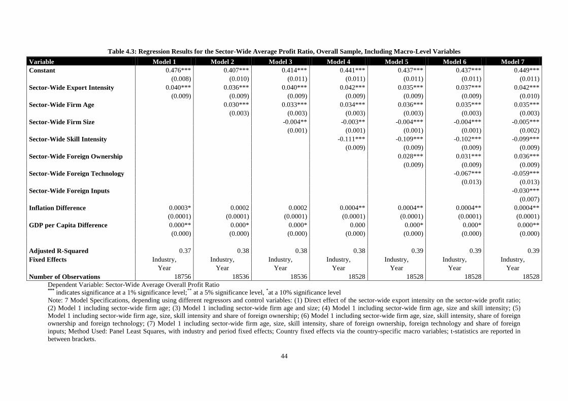
44

Table 4.3: Regression Results for the Sector-Wide Average Profit Ratio, Overall Sample, Including Macro-Level Variables

Dependent Variable: Sector-Wide Average Overall Profit Ratio ***

indicates significance at a 1% significance level;**

at a 5% significance level, *at a 10% significance level

Note: 7 Model Specifications, depending using different regressors and control variables: (1) Direct effect of the sector-wide export intensity on the sector-wide profit ratio;

(2) Model 1 including sector-wide firm age; (3) Model 1 including sector-wide firm age and size; (4) Model 1 including sector-wide firm age, size and skill intensity; (5)

Model 1 including sector-wide firm age, size, skill intensity and share of foreign ownership; (6) Model 1 including sector-wide firm age, size, skill intensity, share of foreign

ownership and foreign technology; (7) Model 1 including sector-wide firm age, size, skill intensity, share of foreign ownership, foreign technology and share of foreign

inputs; Method Used: Panel Least Squares, with industry and period fixed effects; Country fixed effects via the country-specific macro variables; t-statistics are reported in

between brackets.

Variable Model 1 Model 2 Model 3 Model 4 Model 5 Model 6 Model 7

Constant 0.476*** 0.407*** 0.414*** 0.441*** 0.437*** 0.437*** 0.449***

(0.008) (0.010) (0.011) (0.011) (0.011) (0.011) (0.011)

Sector-Wide Export Intensity 0.040*** 0.036*** 0.040*** 0.042*** 0.035*** 0.037*** 0.042***

(0.009) (0.009) (0.009) (0.009) (0.009) (0.009) (0.010)

Sector-Wide Firm Age 0.030*** 0.033*** 0.034*** 0.036*** 0.035*** 0.035***

(0.003) (0.003) (0.003) (0.003) (0.003) (0.003)

Sector-Wide Firm Size -0.004** -0.003** -0.004*** -0.004*** -0.005***

(0.001) (0.001) (0.001) (0.001) (0.002)

Sector-Wide Skill Intensity -0.111*** -0.109*** -0.102*** -0.099***

(0.009) (0.009) (0.009) (0.009)

Sector-Wide Foreign Ownership 0.028*** 0.031*** 0.036***

(0.009) (0.009) (0.009)

Sector-Wide Foreign Technology -0.067*** -0.059***

(0.013) (0.013)

Sector-Wide Foreign Inputs -0.030***

(0.007)

Inflation Difference 0.0003* 0.0002 0.0002 0.0004** 0.0004** 0.0004** 0.0004**

(0.0001) (0.0001) (0.0001) (0.0001) (0.0001) (0.0001) (0.0001)

GDP per Capita Difference 0.000** 0.000* 0.000* 0.000 0.000* 0.000* 0.000**

(0.000) (0.000) (0.000) (0.000) (0.000) (0.000) (0.000)

Adjusted R-Squared 0.37 0.38 0.38 0.38 0.39 0.39 0.39

Fixed Effects Industry, Industry, Industry, Industry, Industry, Industry, Industry,

Year Year Year Year Year Year Year

Number of Observations 18756 18536 18536 18528 18528 18528 18528

45

intensity for the overall sample, it can be inferred that an increase in the aggregate export intensity of

1% gives rise to a significant improvement in the aggregate financial performance of firms of 0.015%.

This result again points at the importance of resource, market share and profit reallocations from less

to more productive firms in explaining the positive impact of trade liberalization on the sector-wide

average performance of firms. It suggests that increasing exports alter firm entry and exit dynamics,

force the least productive firms to leave the market due to increasing competition in both factor and

final goods markets, give rise to a pool of highly productive firms surviving and active in the market

and produce aggregate efficiency improvements. Therefore, the results confirm the earlier conclusion

that there is significant and robust evidence not to reject the first null-hypothesis related to the

complete sample and formulated in section 4.120

.

The empirical findings on the impact of the control variables on the sector-wide average profit

ratio are similar to the earlier described results. The natural logarithm of the sector-wide average firm

age has a significantly positive impact on the aggregate financial performance, which indicates that

sectors with on average more mature firms tend to be more productive due to greater expertise and

experience with respect to efficient production, distribution and marketing strategies. This confirms

the earlier mentioned suggestions proposed by Hannan and Freeman (1984). The natural logarithm of

the sector-wide average firm size has a significantly negative impact on the aggregate financial

performance, which means that sectors with on average larger firms tend to be less productive. This

finding can be explained by the greater difficulties larger firms experience with respect to adjusting to

changing market conditions and supports the conclusions drawn by Tybout et al. (1991). This

inflexibility may serve as a barrier to adapt quickly and efficiently and, therefore, may hamper

improvements in performance. The sector-wide skill intensity has a significantly negative impact on

the sector-wide average financial performance, which can be explained by the higher costs associated

with hiring more skilled workers and confirms the findings by Abowd et al. (1999). In case the higher

costs of hiring skilled workers outweigh the productivity benefits of hiring them, the impact of a

higher sector-wide average skill intensity on the aggregate financial performance may be negative.

The sector-wide average share of foreign ownership has a significantly positive effect on the industry-

wide performance of firms, suggesting that foreign participation positively influences performance due

to technology diffusion and learning effects and confirming earlier documented literature21

. The

impacts of the sector-wide average foreign technology variable and the sector-wide average share of

foreign inputs used in production on the sector-wide average profit ratio are both significantly

negative. These results can be explained by the long time required for efficiently implementing

sophisticated foreign technologies and the higher costs associated with purchasing foreign inputs. Both

these results confirm the findings by Liu (2006).

The macro-level variables included to capture country fixed effects perform well as an

alternative to the conventional country-specific dummies. The explanatory power of the model

including the macro-level variables, with an adjusted R2 in between 0.37 and 0.39, is slightly lower

than to the model including country-specific dummies. The influence of the country-specific inflation

difference on the sector-wide profit ratio is ambiguous. The models that include the sector-wide export

intensity as the regressor and the sector-wide average firm age and/or the sector-wide average firm

20 H0: Trade liberalization has a positive influence on the industry-wide average performance of firms. 21

See, among others, Aitken and Harisson (1999) and Borensztein et al. (1998) for the same argument.

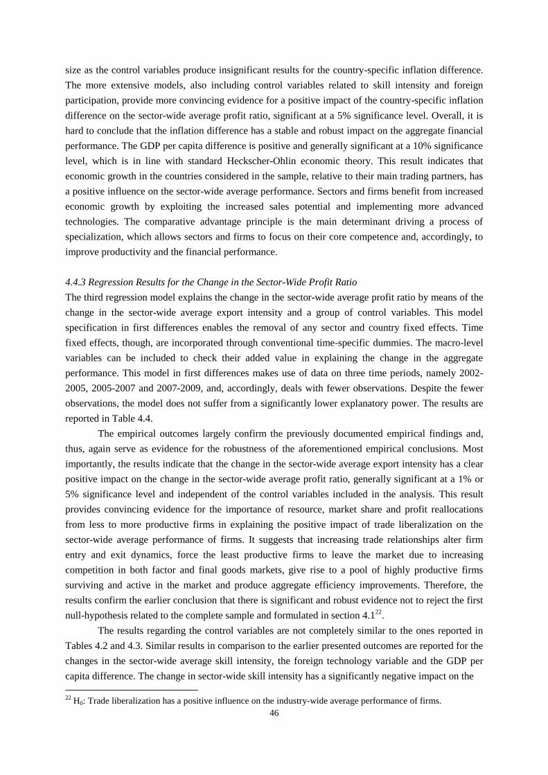
46

size as the control variables produce insignificant results for the country-specific inflation difference.

The more extensive models, also including control variables related to skill intensity and foreign

participation, provide more convincing evidence for a positive impact of the country-specific inflation

difference on the sector-wide average profit ratio, significant at a 5% significance level. Overall, it is

hard to conclude that the inflation difference has a stable and robust impact on the aggregate financial

performance. The GDP per capita difference is positive and generally significant at a 10% significance

level, which is in line with standard Heckscher-Ohlin economic theory. This result indicates that

economic growth in the countries considered in the sample, relative to their main trading partners, has

a positive influence on the sector-wide average performance. Sectors and firms benefit from increased

economic growth by exploiting the increased sales potential and implementing more advanced

technologies. The comparative advantage principle is the main determinant driving a process of

specialization, which allows sectors and firms to focus on their core competence and, accordingly, to

improve productivity and the financial performance.

4.4.3 Regression Results for the Change in the Sector-Wide Profit Ratio

The third regression model explains the change in the sector-wide average profit ratio by means of the

change in the sector-wide average export intensity and a group of control variables. This model

specification in first differences enables the removal of any sector and country fixed effects. Time

fixed effects, though, are incorporated through conventional time-specific dummies. The macro-level

variables can be included to check their added value in explaining the change in the aggregate

performance. This model in first differences makes use of data on three time periods, namely 2002-

2005, 2005-2007 and 2007-2009, and, accordingly, deals with fewer observations. Despite the fewer

observations, the model does not suffer from a significantly lower explanatory power. The results are

reported in Table 4.4.

The empirical outcomes largely confirm the previously documented empirical findings and,

thus, again serve as evidence for the robustness of the aforementioned empirical conclusions. Most

importantly, the results indicate that the change in the sector-wide average export intensity has a clear

positive impact on the change in the sector-wide average profit ratio, generally significant at a 1% or

5% significance level and independent of the control variables included in the analysis. This result

provides convincing evidence for the importance of resource, market share and profit reallocations

from less to more productive firms in explaining the positive impact of trade liberalization on the

sector-wide average performance of firms. It suggests that increasing trade relationships alter firm

entry and exit dynamics, force the least productive firms to leave the market due to increasing

competition in both factor and final goods markets, give rise to a pool of highly productive firms

surviving and active in the market and produce aggregate efficiency improvements. Therefore, the

results confirm the earlier conclusion that there is significant and robust evidence not to reject the first

null-hypothesis related to the complete sample and formulated in section 4.122

.

The results regarding the control variables are not completely similar to the ones reported in

Tables 4.2 and 4.3. Similar results in comparison to the earlier presented outcomes are reported for the

changes in the sector-wide average skill intensity, the foreign technology variable and the GDP per

capita difference. The change in sector-wide skill intensity has a significantly negative impact on the

22 H0: Trade liberalization has a positive influence on the industry-wide average performance of firms.

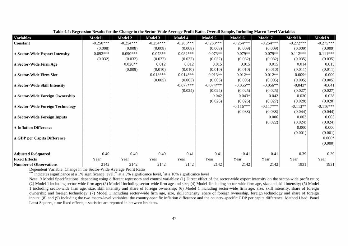
47

Table 4.4: Regression Results for the Change in the Sector-Wide Average Profit Ratio, Overall Sample, Including Macro-Level Variables

Dependent Variable: Change in the Sector-Wide Average Profit Ratio ***

indicates significance at a 1% significance level;**

at a 5% significance level, *at a 10% significance level

Note: 9 Model Specifications, depending using different regressors and control variables: (1) Direct effect of the sector-wide export intensity on the sector-wide profit ratio;

(2) Model 1 including sector-wide firm age; (3) Model 1including sector-wide firm age and size; (4) Model 1including sector-wide firm age, size and skill intensity; (5) Model

1 including sector-wide firm age, size, skill intensity and share of foreign ownership; (6) Model 1 including sector-wide firm age, size, skill intensity, share of foreign

ownership and foreign technology; (7) Model 1 including sector-wide firm age, size, skill intensity, share of foreign ownership, foreign technology and share of foreign

inputs; (8) and (9) Including the two macro-level variables: the country-specific inflation difference and the country-specific GDP per capita difference; Method Used: Panel

Least Squares, time fixed effects; t-statistics are reported in between brackets.

Variables Model 1 Model 2 Model 3 Model 4 Model 5 Model 6 Model 7 Model 8 Model 9

Constant -0.250*** -0.254*** -0.254*** -0.263*** -0.263*** -0.254*** -0.254*** -0.272*** -0.275***

(0.008) (0.008) (0.008) (0.008) (0.008) (0.009) (0.009) (0.009) (0.009)

Δ Sector-Wide Export Intensity 0.092*** 0.090*** 0.078** 0.082*** 0.073** 0.079** 0.079** 0.112*** 0.111***

(0.032) (0.032) (0.032) (0.032) (0.032) (0.032) (0.032) (0.035) (0.035)

Δ Sector-Wide Firm Age 0.020** 0.012 0.012 0.015 0.015 0.015 0.014 0.015

(0.009) (0.010) (0.010) (0.010) (0.010) (0.010) (0.011) (0.011)

Δ Sector-Wide Firm Size 0.013*** 0.014*** 0.013** 0.012** 0.012** 0.009* 0.009

(0.005) (0.005) (0.005) (0.005) (0.005) (0.005) (0.005)

Δ Sector-Wide Skill Intensity -0.077*** -0.074*** -0.055** -0.056** -0.043* -0.041

(0.024) (0.024) (0.025) (0.025) (0.027) (0.027)

Δ Sector-Wide Foreign Ownership 0.042 0.043* 0.042 0.030 0.028

(0.026) (0.026) (0.027) (0.028) (0.028)

Δ Sector-Wide Foreign Technology -0.116*** -0.117*** -0.113** -0.116***

(0.038) (0.038) (0.044) (0.044)

Δ Sector-Wide Foreign Inputs 0.006 0.003 0.003

(0.022) (0.024) (0.024)

Δ Inflation Difference 0.000 0.000

(0.001) (0.001)

Δ GDP per Capita Difference 0.000*

(0.000)

Adjusted R-Squared 0.40 0.40 0.40 0.41 0.41 0.41 0.41 0.39 0.39

Fixed Effects Year Year Year Year Year Year Year Year Year

Number of Observations 2142 2142 2142 2142 2142 2142 2142 1931 1931

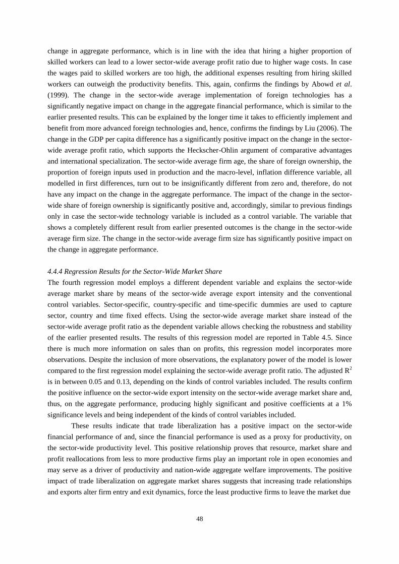
48

change in aggregate performance, which is in line with the idea that hiring a higher proportion of

skilled workers can lead to a lower sector-wide average profit ratio due to higher wage costs. In case

the wages paid to skilled workers are too high, the additional expenses resulting from hiring skilled

workers can outweigh the productivity benefits. This, again, confirms the findings by Abowd et al.

(1999). The change in the sector-wide average implementation of foreign technologies has a

significantly negative impact on change in the aggregate financial performance, which is similar to the

earlier presented results. This can be explained by the longer time it takes to efficiently implement and

benefit from more advanced foreign technologies and, hence, confirms the findings by Liu (2006). The

change in the GDP per capita difference has a significantly positive impact on the change in the sector-

wide average profit ratio, which supports the Heckscher-Ohlin argument of comparative advantages

and international specialization. The sector-wide average firm age, the share of foreign ownership, the

proportion of foreign inputs used in production and the macro-level, inflation difference variable, all

modelled in first differences, turn out to be insignificantly different from zero and, therefore, do not

have any impact on the change in the aggregate performance. The impact of the change in the sector-

wide share of foreign ownership is significantly positive and, accordingly, similar to previous findings

only in case the sector-wide technology variable is included as a control variable. The variable that

shows a completely different result from earlier presented outcomes is the change in the sector-wide

average firm size. The change in the sector-wide average firm size has significantly positive impact on

the change in aggregate performance.

4.4.4 Regression Results for the Sector-Wide Market Share

The fourth regression model employs a different dependent variable and explains the sector-wide

average market share by means of the sector-wide average export intensity and the conventional

control variables. Sector-specific, country-specific and time-specific dummies are used to capture

sector, country and time fixed effects. Using the sector-wide average market share instead of the

sector-wide average profit ratio as the dependent variable allows checking the robustness and stability

of the earlier presented results. The results of this regression model are reported in Table 4.5. Since

there is much more information on sales than on profits, this regression model incorporates more

observations. Despite the inclusion of more observations, the explanatory power of the model is lower

compared to the first regression model explaining the sector-wide average profit ratio. The adjusted R2

is in between 0.05 and 0.13, depending on the kinds of control variables included. The results confirm

the positive influence on the sector-wide export intensity on the sector-wide average market share and,

thus, on the aggregate performance, producing highly significant and positive coefficients at a 1%

significance levels and being independent of the kinds of control variables included.

These results indicate that trade liberalization has a positive impact on the sector-wide

financial performance of and, since the financial performance is used as a proxy for productivity, on

the sector-wide productivity level. This positive relationship proves that resource, market share and

profit reallocations from less to more productive firms play an important role in open economies and

may serve as a driver of productivity and nation-wide aggregate welfare improvements. The positive

impact of trade liberalization on aggregate market shares suggests that increasing trade relationships

and exports alter firm entry and exit dynamics, force the least productive firms to leave the market due

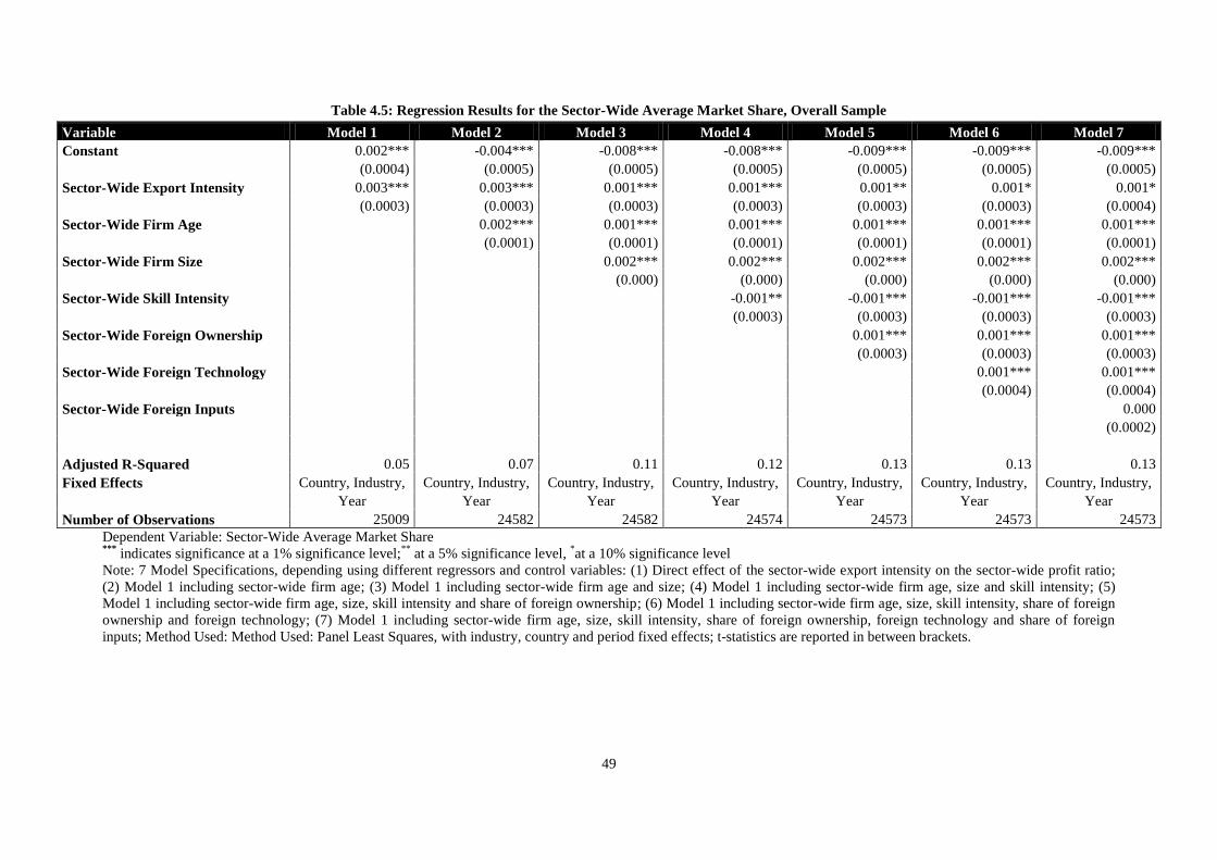
49

Table 4.5: Regression Results for the Sector-Wide Average Market Share, Overall Sample

Dependent Variable: Sector-Wide Average Market Share ***

indicates significance at a 1% significance level;**

at a 5% significance level, *at a 10% significance level

Note: 7 Model Specifications, depending using different regressors and control variables: (1) Direct effect of the sector-wide export intensity on the sector-wide profit ratio;

(2) Model 1 including sector-wide firm age; (3) Model 1 including sector-wide firm age and size; (4) Model 1 including sector-wide firm age, size and skill intensity; (5)

Model 1 including sector-wide firm age, size, skill intensity and share of foreign ownership; (6) Model 1 including sector-wide firm age, size, skill intensity, share of foreign

ownership and foreign technology; (7) Model 1 including sector-wide firm age, size, skill intensity, share of foreign ownership, foreign technology and share of foreign

inputs; Method Used: Method Used: Panel Least Squares, with industry, country and period fixed effects; t-statistics are reported in between brackets.

Variable Model 1 Model 2 Model 3 Model 4 Model 5 Model 6 Model 7

Constant 0.002*** -0.004*** -0.008*** -0.008*** -0.009*** -0.009*** -0.009***

(0.0004) (0.0005) (0.0005) (0.0005) (0.0005) (0.0005) (0.0005)

Sector-Wide Export Intensity 0.003*** 0.003*** 0.001*** 0.001*** 0.001** 0.001* 0.001*

(0.0003) (0.0003) (0.0003) (0.0003) (0.0003) (0.0003) (0.0004)

Sector-Wide Firm Age 0.002*** 0.001*** 0.001*** 0.001*** 0.001*** 0.001***

(0.0001) (0.0001) (0.0001) (0.0001) (0.0001) (0.0001)

Sector-Wide Firm Size 0.002*** 0.002*** 0.002*** 0.002*** 0.002***

(0.000) (0.000) (0.000) (0.000) (0.000)

Sector-Wide Skill Intensity -0.001** -0.001*** -0.001*** -0.001***

(0.0003) (0.0003) (0.0003) (0.0003)

Sector-Wide Foreign Ownership 0.001*** 0.001*** 0.001***

(0.0003) (0.0003) (0.0003)

Sector-Wide Foreign Technology 0.001*** 0.001***

(0.0004) (0.0004)

Sector-Wide Foreign Inputs 0.000

(0.0002)

Adjusted R-Squared 0.05 0.07 0.11 0.12 0.13 0.13 0.13

Fixed Effects Country, Industry, Country, Industry, Country, Industry, Country, Industry, Country, Industry, Country, Industry, Country, Industry,

Year Year Year Year Year Year Year

Number of Observations 25009 24582 24582 24574 24573 24573 24573

50

to increasing competition in both factor and final goods markets, give rise to a pool of highly

productive firms surviving and active in the market and produce aggregate efficiency improvements.

Overall, the results provide significant and robust evidence not to reject the first null-hypothesis

related to the complete sample and formulated in section 4.123

.

The results regarding the control variables provide mixed results in comparison with earlier

reported outcomes and conclusions. In line with the first and second regression model, the natural

logarithm of the sector-wide average firm age has a positive impact on the aggregate financial

performance, significant at a 1% significance level and independent of the control variables included.

This result supports the idea that sectors with on average more mature firms tend to perform better

than sectors with on average younger firms. Firms that have on average been in operations for a longer

period of time may have gained the expertise to produce and sell their products in an efficient and,

accordingly, more profitable way. These kinds of firms may rely upon production techniques,

distribution networks and marketing strategies that have proven to work in the past. Less mature firms

may still be in a process of development, which comes at the cost of efficiency and productivity. This

outcome is line with the suggestions proposed by Hannan and Freeman (1984).

The significantly negative impact of the sector-wide average skill intensity on the aggregate

financial performance confirms the results from the first two regression models. It indicates that,

although skilled labour tends to be more productive than unskilled labour, it can be such that the

productivity and performance related benefits are outweighed by the costs. This result is similar to the

findings by Abowd et al. (1999). The sector-wide average share of foreign ownership has a

significantly positive impact on the sector-wide average market share, which confirms the earlier

described theory that foreign participation and foreign direct investments improve productivity due to

a combination of technology diffusion, productivity spillovers and learning effects.

Contradictory to the outcomes of the first two regression models are the results regarding the

sector-wide average firm size, the sector-wide foreign technology variable and the sector-wide average

share of foreign inputs used in production. The sector-wide average firm size has a significantly

positive impact on aggregate performance, which suggests that sector with on average larger firms

tend to perform better. The sector-wide implementation of foreign technologies has a positive impact

on the sector-wide average market share, which therefore provides additional evidence for the positive

impact of the participation by private foreign individuals, companies or organisations on productivity

already captured by the sector-wide average share of foreign ownership. The sector-wide average

share of foreign supplies used on production turns out to have an insignificant impact on aggregate

performance.

4.4.5 Regression Results for the Sector-Wide Profit Ratio of Exporters

The fifth and final regression model employs a subsample of only exporting firms and explains the

sector-wide average profit ratio by means of the sector-wide average export intensity and the

conventional control variables. Sector-specific, country-specific and time-specific dummies are used

to capture sector, country and time fixed effects. Using the subsample of only exporters instead of the

overall sample as a basis for estimating the regression model allows testing the impact of trade

liberalization on the sector-wide average financial performance of exporters, which according to the

23 H0: Trade liberalization has a positive influence on the industry-wide average performance of firms.

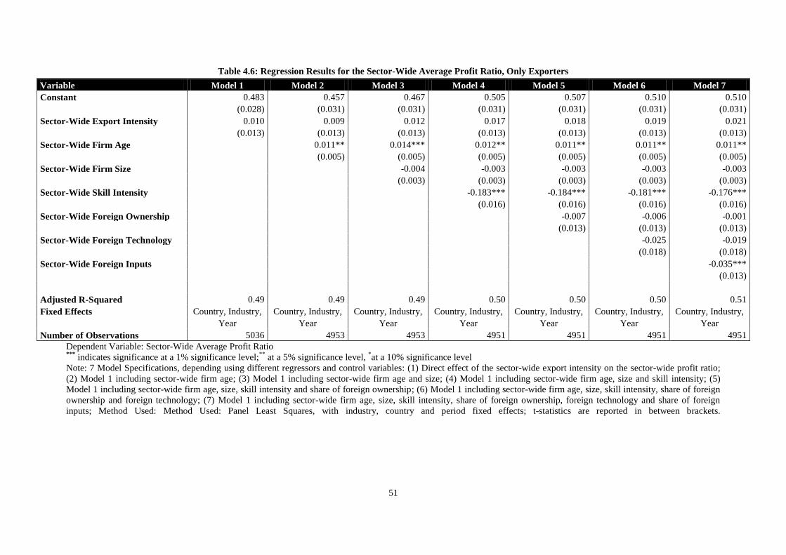
51

Table 4.6: Regression Results for the Sector-Wide Average Profit Ratio, Only Exporters

Dependent Variable: Sector-Wide Average Profit Ratio ***

indicates significance at a 1% significance level;**

at a 5% significance level, *at a 10% significance level

Note: 7 Model Specifications, depending using different regressors and control variables: (1) Direct effect of the sector-wide export intensity on the sector-wide profit ratio;

(2) Model 1 including sector-wide firm age; (3) Model 1 including sector-wide firm age and size; (4) Model 1 including sector-wide firm age, size and skill intensity; (5)

Model 1 including sector-wide firm age, size, skill intensity and share of foreign ownership; (6) Model 1 including sector-wide firm age, size, skill intensity, share of foreign

ownership and foreign technology; (7) Model 1 including sector-wide firm age, size, skill intensity, share of foreign ownership, foreign technology and share of foreign

inputs; Method Used: Method Used: Panel Least Squares, with industry, country and period fixed effects; t-statistics are reported in between brackets.

Variable Model 1 Model 2 Model 3 Model 4 Model 5 Model 6 Model 7

Constant 0.483 0.457 0.467 0.505 0.507 0.510 0.510

(0.028) (0.031) (0.031) (0.031) (0.031) (0.031) (0.031)

Sector-Wide Export Intensity 0.010 0.009 0.012 0.017 0.018 0.019 0.021

(0.013) (0.013) (0.013) (0.013) (0.013) (0.013) (0.013)

Sector-Wide Firm Age 0.011** 0.014*** 0.012** 0.011** 0.011** 0.011**

(0.005) (0.005) (0.005) (0.005) (0.005) (0.005)

Sector-Wide Firm Size -0.004 -0.003 -0.003 -0.003 -0.003

(0.003) (0.003) (0.003) (0.003) (0.003)

Sector-Wide Skill Intensity -0.183*** -0.184*** -0.181*** -0.176***

(0.016) (0.016) (0.016) (0.016)

Sector-Wide Foreign Ownership -0.007 -0.006 -0.001

(0.013) (0.013) (0.013)

Sector-Wide Foreign Technology -0.025 -0.019

(0.018) (0.018)

Sector-Wide Foreign Inputs -0.035***

(0.013)

Adjusted R-Squared 0.49 0.49 0.49 0.50 0.50 0.50 0.51

Fixed Effects Country, Industry, Country, Industry, Country, Industry, Country, Industry, Country, Industry, Country, Industry, Country, Industry,

Year Year Year Year Year Year Year

Number of Observations 5036 4953 4953 4951 4951 4951 4951

52

second hypothesis formulated in section 4.1 should be ambiguous and insignificant24

. The regression

based on only exporters incorporates fewer observations. The explanatory power, though, is relatively

high in comparison with the earlier discussed models, with an adjusted R2 in between 0.49 and 0.51.

The results of this regression model are reported in Table 4.6.

By studying the reported results, it can be concluded that the sector-wide export intensity has

an insignificant impact on the sector-wide average profit ratio of exporters, independent of the type of

control variables included. This result indicates that trade liberalization has an ambiguous and

insignificant influence on the aggregate performance of exporters and, therefore, supports the

theoretical predictions. Theoretically, it has been argued that in an open economy setting only the most

productive firms, i.e. firms with a productive parameter that is equal to or greater than the cut-off

productive parameter determining a firm’s export status, enter the export market. This export market

selection effect causes a type of Darwinian evolution to take place within an industry. Only the most

efficient firms experience higher market shares and higher profits by serving both the domestic market

and the foreign market. Some less efficient firms are productive enough to export and, accordingly,

experience an increase in market share, but at the same time suffer a profit loss. Combined, it can be

inferred that the impact of trade liberalization on the financial performance of exporters is ambiguous

and insignificant. The insignificant relationship between the sector-wide average export intensity and

the aggregate performance of exporters confirms this theoretical result. It can thus be concluded that

there is significant and robust evidence not to reject the exporters-specific null-hypothesis formulated

in section 4.1.

The results regarding the control variables are generally similar to the earlier reported

outcomes and conclusions. The natural logarithm of the sector-wide average firm age has a

significantly positive impact on the aggregate performance of exporters, which confirms the earlier

formulated idea that sectors with on average more mature firms tend to perform better than sectors

with on average younger firms and supports the suggestions by Hannan and Freeman (1984). Firms

that have on average been in operations for a longer period of time may have gained the expertise to

produce and sell their products in an efficient and, accordingly, more profitable way. These kinds of

firms may rely upon production techniques, distribution networks and marketing strategies that have

proven to work in the past. Less mature firms may still be in a process of development, which comes

at the cost of efficiency and productivity. The natural logarithm of the sector-wide average firm size

has an insignificant impact on the sector-wide average profit ratio of exporters, which contradicts

earlier results. This may be due to a greater degree of homogeneity among exporters. The sector-wide

average skill intensity has a significantly negative impact on the aggregate performance of exporters,

which supports the idea that the costs of hiring a higher proportion of skilled labour can outweigh the

benefits, negatively affecting the sector-wide average performance. This result is in line with the

findings by Abowd et al. (1999). The results regarding the control variables capturing the influence of

private foreign individuals are mixed. The sector-wide average share of foreign ownership and the

sector-wide average foreign technology variable are both insignificantly different from zero, which

contradicts the outcomes resulting from other regression models incorporating the complete dataset.

The sector-wide average share of foreign inputs is significantly negative, which is in line with the

24 H0: Trade liberalization has an ambiguous and insignificant influence on the industry-wide average

performance of exporters.

53

other regression models. This result may indicate that foreign inputs used in production can only be

purchased at a higher cost due to for example transportation expenses and tariffs, which has a negative

impact on the financial performance of exporters.

4.5 Trade Liberalization and Performance: A Different Perspective

The economic impact of trade liberalization cannot necessarily be explained by a single theory. The

process of within industry resource, market share and profit reallocations from less to more productive

firms is a useful theory in explaining the influence of trade liberalization on aggregate performance

and identifying a unique contributor to country-wide welfare. As outlined in section 2.1, other theories

focus on explaining the impact of trade liberalization through processes of within firm productivity

improvements. In particular, Grossman and Helpman (1991, 1993) analytically emphasize the

importance of knowledge spillover effects resulting from the international trade of final and

intermediate products, whereas Aghion et al. (2005) argue that trade liberalization incentivizes firms

to invest more in innovation. Goh (2000), related to Aghion et al. (2005), shows that trade

liberalization tends to reduce the opportunity cost of technological effort and to increase the

willingness to adopt new, more efficient technologies. This has a positive impact on firm efficiency

and productivity. Holmes and Schmitz (2001) assess the link between trade liberalization and firm

productivity by proving that increased exposure to trade makes firms spend more time on productive

activities rather than unproductive activities. Tybout and Westbrook (1995) provide an overview of the

sources of economies of scale that, through increased openness to trade, improve firm efficiency and

productivity.

To empirically investigate the importance of within firm productivity changes in explaining

the economic impacts of trade liberalization, a panel regression model is estimated, regressing the

firm-specific financial performance on the sector-wide average export intensity and a series of control

variables capturing firm characteristics. Analytically, the model looks as follows:

(4.8)

where PRijt is the profit ratio of firm i in country j at time t and Expijt is the sector-wide export intensity

characterizing sector s in which firm i in country j at time t is active. Sector-wide, export intensities

are used instead of firm-specific export intensities as trade liberalization is a macroeconomic

phenomenon and, thus, is best captured by sector-wide economic developments. x’ijt is a vector of

control variables, including the firm characteristics related to firm age, size, foreign participation and

influence and skill intensity. ΔInflationjt is the inflation difference between country j and five of its

main trading partners at time t, and ΔGDPpcjt is the GDP per capita difference between country j and

five of its main trading partners at time t. These two macro variables are used to capture country-

specific fixed effects. δi and δt are firm-specific and time-specific dummies, capturing firm and time

fixed effects.

The results are reported in Table 4.7 and provide some interesting outcomes. In particular, it

can be seen that the sector-wide average export intensity has a positive impact on the firm-specific

financial performance, significant at a 5% significance level and independent of the exact model

'

1 1 2 , ijt sjt ijt jt jt i t ijtPR Exp x Inflation GDPpc

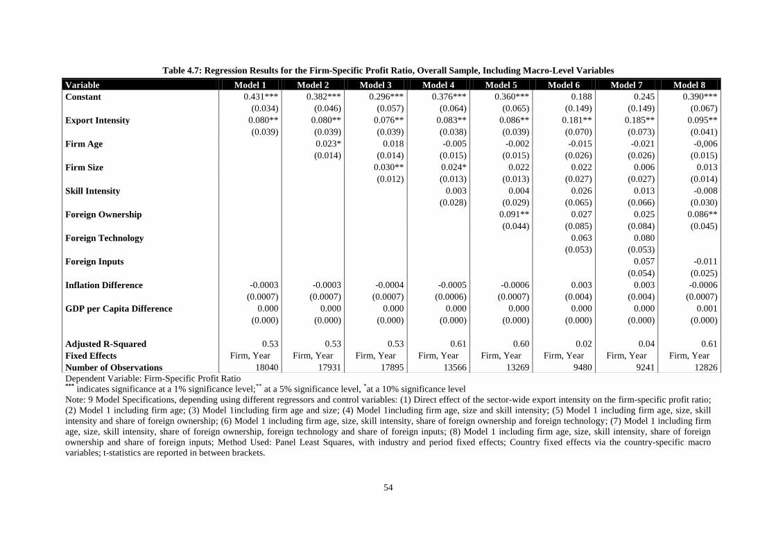
54

Table 4.7: Regression Results for the Firm-Specific Profit Ratio, Overall Sample, Including Macro-Level Variables

Dependent Variable: Firm-Specific Profit Ratio ***

indicates significance at a 1% significance level;**

at a 5% significance level, *at a 10% significance level

Note: 9 Model Specifications, depending using different regressors and control variables: (1) Direct effect of the sector-wide export intensity on the firm-specific profit ratio;

(2) Model 1 including firm age; (3) Model 1including firm age and size; (4) Model 1including firm age, size and skill intensity; (5) Model 1 including firm age, size, skill

intensity and share of foreign ownership; (6) Model 1 including firm age, size, skill intensity, share of foreign ownership and foreign technology; (7) Model 1 including firm

age, size, skill intensity, share of foreign ownership, foreign technology and share of foreign inputs; (8) Model 1 including firm age, size, skill intensity, share of foreign

ownership and share of foreign inputs; Method Used: Panel Least Squares, with industry and period fixed effects; Country fixed effects via the country-specific macro

variables; t-statistics are reported in between brackets.

Variable Model 1 Model 2 Model 3 Model 4 Model 5 Model 6 Model 7 Model 8

Constant 0.431*** 0.382*** 0.296*** 0.376*** 0.360*** 0.188 0.245 0.390***

(0.034) (0.046) (0.057) (0.064) (0.065) (0.149) (0.149) (0.067)

Export Intensity 0.080** 0.080** 0.076** 0.083** 0.086** 0.181** 0.185** 0.095**

(0.039) (0.039) (0.039) (0.038) (0.039) (0.070) (0.073) (0.041)

Firm Age 0.023* 0.018 -0.005 -0.002 -0.015 -0.021 -0,006

(0.014) (0.014) (0.015) (0.015) (0.026) (0.026) (0.015)

Firm Size 0.030** 0.024* 0.022 0.022 0.006 0.013

(0.012) (0.013) (0.013) (0.027) (0.027) (0.014)

Skill Intensity 0.003 0.004 0.026 0.013 -0.008

(0.028) (0.029) (0.065) (0.066) (0.030)

Foreign Ownership 0.091** 0.027 0.025 0.086**

(0.044) (0.085) (0.084) (0.045)

Foreign Technology 0.063 0.080

(0.053) (0.053)

Foreign Inputs 0.057 -0.011

(0.054) (0.025)

Inflation Difference -0.0003 -0.0003 -0.0004 -0.0005 -0.0006 0.003 0.003 -0.0006

(0.0007) (0.0007) (0.0007) (0.0006) (0.0007) (0.004) (0.004) (0.0007)

GDP per Capita Difference 0.000 0.000 0.000 0.000 0.000 0.000 0.000 0.001

(0.000) (0.000) (0.000) (0.000) (0.000) (0.000) (0.000) (0.000)

Adjusted R-Squared 0.53 0.53 0.53 0.61 0.60 0.02 0.04 0.61

Fixed Effects Firm, Year Firm, Year Firm, Year Firm, Year Firm, Year Firm, Year Firm, Year Firm, Year

Number of Observations 18040 17931 17895 13566 13269 9480 9241 12826

55

specification. This result indicates that trade liberalization positively influences firm productivity and

performance through processes of within firm changes and confirms the general consensus among

researchers. Possible explanations for this positive result include the exploitation of economies of

scale, knowledge spillovers, learning effects, the implementation of more advanced foreign

technologies, and increased incentives to innovate and to spend more time on productive activities

instead of on unproductive activities. It can be concluded that trade liberalization, next to within

industry reallocations that positively influence aggregate performance, also causes within firm changes

that improve efficiency and productivity.

The results regarding the control variables are generally insignificant, which is contradictory

to the earlier reported outcomes. Firm age, firm size, the firm-specific skill intensity, the foreign

technology variable and the use of foreign inputs seem not to have a significant impact on the financial

performance of a firm. A complete model specification either including or excluding the foreign

technology variable, being models 7 and 8 respectively, is estimated to overcome the econometric

problem of estimating a model with insufficient information on the firm-specific use of foreign

technologies. The model excluding the foreign technology variable has a far greater explanatory

power, as can be seen by the adjusted R2 of 0.61, and provides more stable statistical outcomes

compared to the model including the foreign technology variable. The only variable that has a fairly

stable and significant impact on firm performance is the share of foreign ownership. The firm-specific

share of foreign ownership has a positive impact on firm performance, significant at a 5% significance

level. This outcome is in line with previous literature on foreign participation, foreign direct

investments and the productivity of firms. Most studies show productivity improvements following

foreign participation and foreign direct investments due to a combination of technology diffusion,

productivity spillovers and learning effects (Aitken and Harisson, 1999).

4.6. Overview of the Empirical Results

The main empirical results, based on the different regression models, can be summarized as follows:

There is a significantly positive relationship between the sector-wide average export intensity

and the sector-wide average performance of firms, independent of the proxy used for financial

performance. This result supports the hypothesis that trade liberalization has a positive

influence on the industry-wide average performance of firms.

There is an insignificant relationship between the sector-wide average export intensity and the

aggregate financial performance of exporters. This result supports the hypothesis that trade

liberalization has no impact on the average performance of exporters.

Overall, these two results support the importance of resource, market share and profit

reallocations from less to more productive firms in explaining the positive influence of trade

liberalization on the industry-wide average performance of firms.

Regarding the control variables included in the empirical analysis, the overall results give rise to the

following conclusions:

Sectors with on average more mature firms tend to perform better and be more productive.

The sector-wide average firm size has an ambiguous effect on aggregate performance.

56

Sectors with on average a higher proportion on skilled workers being employed tend to

perform worse, which can be the results of the higher wages of skilled workers that outweigh

the productivity benefits.

Sector-wide foreign ownership has a positive influence on aggregate performance, considering

both the sample of all firms included in the dataset and the subsample of only exporters. This

result is in line with previous literature, pointing at the positive impact of foreign ownership

on performance through technology diffusion and spillover effects.

The impact of the sector-wide implementation of foreign technologies is indeterminate, which

can be the result of the relatively short time period considered.

The sector-wide use of foreign supplies tends to have a negative impact on the sector-wide

average financial performance, which may be due to the higher costs associated with

purchasing foreign inputs.

57

5. Conclusion

Many researchers have attempted to specify the mechanisms that underlie the generally positive

relationship between trade liberalization and firm and aggregate productivity. Suggested mechanisms

include economies of scale, knowledge spillovers and increased incentives to devote more time to

innovative and productive activities.

This research paper theoretically and empirically investigates the importance of resource,

market share and profit reallocation mechanisms in explaining the impact of trade liberalization on the

sector-wide average performance of firms. The theoretical analysis largely builds upon the pioneering

research by Melitz (2003), which assesses the role of trade liberalization as a catalyst for inter-firm

resource, market share and profit reallocations within an industry. Melitz (2003) is one of the first

researchers to develop a theoretical, dynamic industry model that includes Dixit-Stiglitz preferences,

increasing returns to scale and firm heterogeneity in the total factor productivity parameter. The

theoretical model developed in this paper incorporates many of the features of the model by Melitz

(2003) and, in addition to Melitz (2003), argues that firm productivity can objectively be proxied by

indicators of financial performance. By comparing the market entry dynamics in a closed economy

setting and in an open economy setting, the theoretical analysis gives rise to three clear results. Firstly,

the theoretical results suggest that trade liberalization has a positive influence on the industry-wide

average productivity and financial performance level through processes of resource, market share and

profit reallocations from less to more productive firms. This result can be explained by the

combination of a domestic market and an export market selection effect. Since exposure to trade

increases the expected profits conditional on successful market entry, more firms (both domestic new

entrants and foreign competitors) enter the domestic market, which intensifies competition in factor

and final goods markets. Firms will serve smaller market shares and earn lower profits, which allows

only the more productive firms to survive in the market and forces the less productive firms to exit.

Successfully entering the foreign market is only achieved by the most productive firms, as exporting

goods and services is characterized by additional transportation expenses and fixed costs for serving

the foreign market. Secondly, it is shown that in an open economy setting there is a direct positive

relationship between the sector-wide average financial performance of firms and the aggregate

productivity level, which supports the idea that financial performance is a reliable, objective and

accurately measurable proxy of productivity. Thirdly, the theoretical results suggest that trade

liberalization has an ambiguous and insignificant impact on the sector-wide average productivity and

financial performance of exports. In particular, trade liberalization has two contradictory effects

among exporters. The most productive exporters gain in both market shares and profits. Some slightly

less productive firms, though, will continue to export, but will experience financial difficulties.

Overall, the impact of trade liberalization on the aggregate performance of exporters can be concluded

to be ambiguous and insignificant. These theoretical results are used to formulate two hypotheses on

the impact of trade liberalization on the sector-wide average performance of firms and exporters,

respectively, which are tested empirically.

The empirical analysis employs firm-level data on 27 Eastern European and Central Asian

countries over the period 2002-2009, provided by the Business Environment and Enterprise

Performance Surveys (BEEPS) and constructed by the joint effort of the World Bank and the

European Bank for Reconstruction and Development. The complete dataset consists of 23,570 firms,

58

active in 503 4-digit ISIC code specified sectors over the years 2002, 2005, 2007 and 2009. The

information gathered covers many different aspects of a firm used to calculate the various sector-level

variables, including general information, infrastructure and services, sales and supplies, the degree of

competition, capacity, land and permits, crime, finance, business-government relations, labour, the

business environment, and performance. Different econometric estimation procedures are followed,

depending on the sample and the dependent variable used and the kind of fixed effects estimation

technique employed. The panel regression results confirm the hypotheses formulated on the basis of

the theoretical analysis. In particular, the outcomes reveal a stable, robust and significantly positive

impact of the sector-wide export intensity on the industry-wide average financial performance of

firms, measured by means of the aggregate profit ratio or the sector-wide market share. This result

suggests that trade liberalization has a structurally positive influence on the aggregate financial

performance of firms through processes of resource, market share and profit reallocations.

Additionally, the outcomes of the panel regression model employing a subsample of only exporting

firm show that there is an insignificant relationship between the sector-wide average export intensity

and the aggregate financial performance of exporters. This result supports the theoretical hypothesis

that trade liberalization has no impact on the average performance of exporters. Interesting results

regarding the control variables include the fact that sectors with on average more mature firms tend to

perform better possibly due to greater expertise and experience and that sectors with on average a

higher proportion on skilled workers being employed tend to perform worse, which can be the result

of the higher wages paid to skilled workers that outweigh the productivity benefits. Sectors with a high

degree of foreign ownership tend to perform better possible due to technology diffusion, knowledge

spillovers and learning effect, whereas sectors that use a high proportion of foreign supplies tend to

perform worse possible due to the higher costs associated with purchasing foreign inputs. Overall, the

empirical results prove the significant importance of resource, market share and profit reallocations

from less to more productive firms in explaining the positive influence of trade liberalization on the

industry-wide average performance of firms. This conclusion proves the effectiveness of classic, open

economy market mechanisms in improving aggregate firm productivity and, accordingly, general

economic performance through the creation of ‘healthy’ competitive pressures. Progressive reforms

focused on further liberalization and increasing competition should therefore be embraced rather than

be abandoned by policymakers in periods of crises.

Even though the results provide satisfactory insights into the overall effect of trade

liberalization through firm heterogeneity in the total factor productivity parameter, there is plenty of

room for further research and empirical refinements. Instead of using the survey information to

estimate sector-wide export intensities, it is possible to calculate exact sector-wide export intensities

using the information on total sector-wide exports and sales from the International Trade Centre. This

allows a more specific definition of different sectors on the basis of highly disaggregated product and

industry classifications and, thus, may give a more precise proxy for the macroeconomic process of

trade liberalization. Additionally, instead of using data on just four years, more historical export data

can be used to assess the longer term sector-wide, economic effects of trade liberalization. This is

particularly relevant since the impacts of resource, market share and profit reallocations on the ecnomy

occur over a long period of time.

59

6 References

Abowd, J.M., Kramarz, F. and Margolis, D.N. (1999), ‘High Wage Workers and High Wage Firms’,

Econometrica, 67, 251-333

Aghion, P., Burgess, R., Redding, S. and Zilibotti, F. (2005), ‘Entry Liberalization and Inequality in

Industrial Performance’, Journal of the European Economic Association, 3, 291-302

Amiti, M. and Konings, J. (2007), ‘Trade Liberalization, Intermediate Inputs, and Productivity:

Evidence from Indonesia’, The American Economic Review, 97, 1611-1638

Aitken, B.J. and Harrison, A.E. (1999), ‘Do Domestic Firms Benefit from Direct Foreign Investment?

Evidence from Venezuela’, American Economic Review, 89, 605-618

Aw, B.Y., Chen, X. and Roberts, M.J. (2001), ‘Firm-Level Evidence on Productivity Differentials and

Turnover in Taiwanese Manufacturing’, Journal of Development Economics, 66, 51-86

Baily, M.N. and Farrell, D. (2005), ‘A Road Map for European Economic Reform: The Region Must

Do Away with Restrictive Regulations and Embrace Competition’, The McKinsey Quarterly,

The McKinsey Global Institute, McKinsey & Company

Berk, J. and DeMarzo, P. (2007), ‘Corporate Finance’, Pearson Education: Pearson International

Edition

Borensztein, E., De Gregori, J. and Lee, J.W. (1998), ‘How Does Foreign Direct Investment Affect

Economic Growth?’, Journal of International Economics, 45, 115-135

Blundell, R., Griffith, R. and Van Reenen, J. (1999), ‘Market Share, Market Value, and Innovation in

a Panel of British Manufacturing Firms’, Review of Economic Studies, 66, 529-554

Dixit, A.K. and Stiglitz, J.E. (1977), ‘Monopolistic Competition and Optimum Product Diversity’, The

American Economic Review, 65, 297-308

Dornbusch, R. and Edwards, S. (1994), ‘Exchange Rate Policy and Trade Strategy’, in Bosworth, B.,

Dornbush, R. and Labán, R., The Chilean Economy: Policy Lessons and Challenges,

Brookings Institution Press

European Commission. (2012), ‘Eurostat Statistics Database: The Real GDP Growth Rate’, Online

Resource Available at: http://epp.eurostat.ec.europa.eu/

Fernandes, A.M. (2007), ‘Trade Policy, Trade Volumes and Plant-Level Productivity in Colombian

Manufacturing Industries’, Journal of International Economics, 71, 52-71

Goh, A-T. (2000), ‘Opportunity Cost, Trade Policies and the Efficiency of Firms, Journal of

Development Economics, 62, 363-383

Grossman, G.M. and Helpman, E. (1990), ‘The “New” Growth Theory: Trade, Innovation, and

Growth”, The American Economic Review, 80, 86-91

Grossman, G.M. and Helpman, E. (1993), ‘Innovation and Growth in the Global Economy’, MIT

Press

60

Hannan, M.T. and Freeman, J. (1984), ‘Structural Inertia and Organizational Change’, American

Sociological Review, 49, 149-164

Harrison, A.E. (1994), ‘Productivity, Imperfect Competition and Trade Reform: Theory and

Evidence’, Journal of International Economics, 39, 53-73

Holmes, T.J. and Schmitz Jr., J.A. (2001), ‘A Gain from Trade: From Unproductive to Productive

Entrepreneurship’, Journal of Monetary Economics, 47, 417-446

International Trade Centre. (2012), ‘Trade Statistics for International Business Development’, Trade

Map: International Trade Statitics, Online Resource Available at: http://www.trademap.org/

Levinsohn, J. and Petrin, A. (2003), ‘Estimating Production Functions Using Inputs to Control for

Unobservables’, The Review of Economic Studies, 70, 317-341

Liu, Z. (2006), ‘Foreign Direct Investment and Technology Spillovers: Theory and Evidence’, Journal

of Development Economics, 85, 176-193

Melitz, M.J. (2003), ‘The Impact of Trade on Intra-Industry Reallocations and Aggregate Industry

Productivity’, Econometrica, 71, 1695-1725

Nataraj, S. (2011), ‘The Impact of Trade Liberalization on Productivity: Evidence from India’s Formal

and Informal Manufacturing Sectors’, Journal of International Economics, 85, 292-301

Olley, G.S. and Pakes, A. (1996), ‘The dynamics of Productivity in the Telecommunications

Equipment Industry’, Econometrica, 64, 1263-1297

Pavcnik, N. (2002), ‘Trade Liberalization, Exit, and Productivity Improvements: Evidence from

Chilean Plants’, The Review of Economic Studies, 69, 245-276

Roberts, M.J. and Tybout, J.R. (1996), ‘Industrial Evolution in Developing Countries: Micro Patterns

of Turnover, Productivity, and Market Structure’, Published for the World Bank, Oxford

University Press

Tybout, J.R., De Melo, J. and Corbo, V. (1991), ‘The Effects of Trade Reforms on Scale and

Technical Efficiency: New Evidence from Chile’, Journal of International Economics, 31,

231-250

Tybout, J.R. and Westbrook, M.D. (1995), ‘Trade Liberalization and the Dimensions of Efficiency

Change in Mexican Manufacturing Industries’, Journal of International Economics, 39, 53-78

Verbeek, M. (2008), ‘A Guide to Modern Econometrics’, John Wiley & Sons Ltd, 3rd

Edition

World Bank. (2012), ‘Business Environment and Enterprise Performance Surveys (BEEPS): Eastern

Europe and Central Asia’, The World Bank & The European Bank for Reconstruction and

Development, Online Resource Available at: http://www.enterprisesurveys.org/

World Bank. (2012), ‘World Bank Development Indicators & Global Development Finance 2011’,

World Bank Databank, Online Resource Available at: http://www.databank.worldbank.org/

61

1 1

1

2 1 2 2

2

10.p q q q

q

7 Appendix

Proof A1: Equation 3.2, The Price per Unit Utility P

The utility function, assuming Dixit-Sitglizt prefences, a constant elasticity of substitution and two

varieties, equals:

(7.1)

Optimizing utility is similar to minimizing the costs. Accordingly, to determine the optimal quantities

of q1 and q2 consumed, the following Lagrangian can be formulated:

(7.2)

The first order conditions of equation 7.2 with respect to q1 and q2 are equal to:

(7.3)

and

(7.4)

Dividing equation 7.3 by 7.4 and rewriting yields the following expression for q1:

(7.5)

Plugging equation 7.5 into the side constraint of equation 7.2 allows deriving the optimal quantity

consumed of variety q2 as a function of p1 and p2:

(7.6)

Similarly, the optimal quantity consumed of variety q1 is equal to:

(7.7)

Combining equations 7.6 and 7.7 yields a total expenditure function:

(7.8)

By assuming that the elasticity of substitution between varieties is σ = 1/(1-ρ) > 1, equation 7.8 can be

simplified to:

(7.9)

In case of infinitely many varieties, equation 7.9 is equal to:

1

1 2 .U q q

1

1 1 2 2 1 21 .p q p q q q

1 1

1

1 1 2 1

1

10p q q q

q

11

11 2

2

.p

q qp

1

1 1 1

1

2 1 2 2 .q p p p

1

1 1 1

1

1 1 2 1 .q p p p

1 1

1 1 1 1 1 1

1 1 11 1

1 2 2 1 1 2 .P p p p p p p

1

11 1

1 2 .P p p

62

(7.10)

Proof A2: Equation 3.8, The Marginal Revenue Function

The total demand for a single variety φ, as in equation 3.5, is equal to:

(7.11)

Equation 7.11 can be used to determine a function for p(φ). This function is equal to:

(7.12)

The total revenues earned per firm, being the product of the price charged and the quantity sold, are

equal to:

(7.13)

The marginal revenue function, defined as the first order derivative of a firm’s revenues with respect

to the quantity sold, then is equal to:

(7.14)

Proof A3: Equation 3.9, The Marginal Cost Function

The total costs faced by a firm consist of fixed and variable production costs. Analytically, the total

costs function can be expressed as follows:

(7.15)

The marginal cost function, defined as the first order derivative of a firm’s total costs with respect to

the quantity sold, then is equal to:

(7.16)

Proof A4: Equation 3.12, The Profit Function

Total profits are equal to the difference between total revenues and total costs, consisting of variable

and fixed costs. Analytically, total profits can be written as:

(7.17)

Since the optimal price charged is equal to a mark-up over marginal costs, the inverse of the optimal

pricing rule, as in equation 3.11, can be used to rewrite equation 7.17 as follows:

11

1.P p d

1 .q I P p

111 .p I P q

1 111 .r I P q

111 1 1 1 1 .r

MR I P q pq

1.TC w f w q

1.

TCMC w

q

.p q c q f

63

(7.18)

Rearranging terms yields:

(7.19)

Equation 7.19 can further be simplified so that the profit function as in equation 3.12 is obtained:

(7.20)

Proof A5: Equation 3.26, The Per Period Equivalent of the Fixed sunk Market Entry Cost

A firm is indifferent between paying fe upon market entry or the per period equivalent of fe in each

period the firm expects to survive. Analytically, this implies:

(7.21)

Multiplying equation 7.21 by (1-θ) yields:

(7.22)

Taking the difference between 7.21 and 7.22 yields the relationship between fe and fPPE:

(7.23)

Proof A6: Equation 3.30 and 3.51, The Transformed Zero Cut-off Profit Condition

By using equation 3.15, the ratio of the revenues earned by a firm with the cut-off productivity level

and the revenues earned by a firm with the average productivity level can be determined:

(7.24)

Equation 7.24 can be rearranged into a function for the cut-off revenue level:

(7.25)

The equation for the cut-off revenue level can be plugged into the original zero cut-off profit

condition. This yields:

(7.26)

Equation 7.26 can be rewritten into the transformed zero cut-off profit condition:

1

.p q p q f

1

1 .p q f

.p q r

f f

2 3

1 1 1 ...e PPE PPE PPE PPEf f f f f

2 3 4

1 1 1 1 1 ...e PPE PPE PPE PPEf f f f f

.PPE ef f

1

.r

r

1

.r r

1

.

r

f

64

(7.27)

Proof A7: Equation 3.31, The Transformed Free Entry Condition

The average profit level is equal to:

(7.28)

The function for the average profit level can be plugged into the original free entry condition. This

yields:

(7.29)

Using the transformed zero cut-off profit condition to substitute for the average revenue level in

equation 7.29 yields a more comprehensive free entry condition:

(7.30)

Equation 7.30 can further be simplified into the transformed free entry condition, which, as in equation

3.31, is equal to:

(7.31)

Proof A8: Equation 3.49 and 3.50, The Export Market Cut-Off Productivity Level

The ratio of the zero cut-off profit condition for the export and the domestic market is equal to:

(7.32)

The symmetry condition implies that all exogenous variables are similar, both domestically and

abroad. Hence, P = PF and I = IF. This means that these variables cancel out. Accordingly, equation

7.32 can be simplified to equation 3.49:

(7.33)

Substituting the optimal prices charged domestically and abroad, as in equations 3.11 and 3.32, into

equation 7.33 yields:

(7.34)

1

.

r f

.r

f

1 .e

rG f f

1

1 .e

f

G f f

1

1 1 .eG f f

11 1

11

.x F F x

p P I f

fp P I

1

1

1.

x xp f

fp

1

1

1

1.

1

1

x xf

f

65

Since both the numerator and the denominator of the left-hand side of equation 7.34 depend on the

mark-up over marginal costs, the mark-up can be removed from the equation. Equation 7.34 can then

be simplified to:

(7.35)

Rearranging terms in equation 7.35 yields a function for the export market cut-off productivity level,

explained by means of the domestic market cut-off productivity level:

(7.36)

Proof A9: Equation 3.52, The Transformed Zero Cut-off Profit Condition for the Foreign

Market

Deriving the transformed zero cut-off profit condition for the foreign market follows the exact same

procedure as the procedure followed for the derivation of the zero cut-off profit condition for the

domestic market. Using equation 3.15, the ratio between the revenues earned by an exporter with the

cut-off productivity level and the revenues earned by an exporter with the average productivity level

can be determined:

(7.37)

Equation 7.37 can be rearranged into a function for the cut-off revenue level:

(7.38)

The equation for the cut-off revenue level can be plugged into the original zero cut-off profit

condition. This yields:

(7.39)

Equation 7.39 can be rewritten into the transformed zero cut-off profit condition for the foreign

market:

(7.40)

Proof A10: An Example of the Derivation of the Closed Economy and the Open Economy

Equilibrium

This example makes the assumptions of a constant elasticity of substitution σ = 2 and a uniform

distribution of the productivity parameter φ on the interval [ ; ]. The conditional distribution μ(φ) of

productivity levels characterizing firms that are active in the market, accordingly, is equal to:

1

1 .x

x

f

f

11

.xx

f

f

1

.x x

x

r

r

1

.xx x

x

r r

1

.

xx

x

x

r

f

1

.xx x

x

r f

66

(7.41)

The average productivity parameter, in accordance with its definition in equation 3.22, is equal to:

(7.42)

Because of the assumption of a uniform distribution of the productivity parameter φ, the function for

the average productivity parameter can be simplified to:

(7.43)

The probability of successful market entry equals:

(7.44)

By combining equations 7.43 and 7.44, the free entry condition can be completed in accordance with

equation 3.31. This yields:

(7.45)

Equation 7.45 characterizes the closed economy equilibrium and can be used to perform the

comparative statics exercises discussed in section 3.3.2. In an open economy setting, the free entry

condition consists of two components, namely the expected profits conditional on successful domestic

market entry and the expected profits conditional successful export market entry. The probability of

successful domestic market entry equals:

(7.46)

The average productivity level in the domestic market is similar to equation 7.43 and equals:

(7.47)

The probability of successful export market entry equals:

(7.48)

The average productivity level in the export market is similar to equation 7.43 and equals:

(7.49)

1

.

1.d

1

.2

1 1 .G

1

2 1 .ef

f

1 .G

1

.2

1 .xxG

1

.2

x x

67

The link between the export market cut-off productivity level and the domestic market cut-off

productivity level, as in equation 3.50, can be expressed as follows:

(7.50)

By combining equations 7.46, 7.47, 7.48, 7.49 and 7.50, the open economy, free entry condition can

be completed in accordance with equation 3.53. This yields:

(7.51)

In comparison with the closed economy equilibrium, equation 7.51 contains an additional positive

term, which implies that trade liberalization has a positive impact on the cut-off productivity level and

the sector-wide average productivity level. Namely, to maintain balance in equation 7.51, the left-hand

side of the equation needs to decrease, which happens only after an increase in the cut-off productivity

level and, accordingly, the average productivity level. This results points at the importance of

resource, market share and profit reallocations in explaining the effect of trade liberalization on sector-

wide average productivity, which into detail is discussed in section 3.4.5.

.xx

f

f

1 1 .2

2

x x

x e

x

f f

f ff f f

f

f

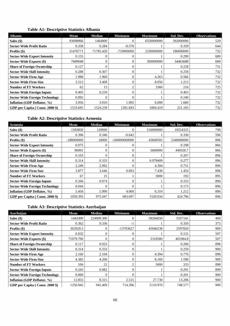
68

Table A1: Descriptive Statistics Albania

Albania Mean Median Minimum Maximum Std. Dev. Observations

Sales ($) 93698966 1464000 0 6550000000 392000000 529

Sector-Wide Profit Ratio 0.358 0.284 -0.570 1 0.339 644

Profits ($) 31476771 71785.420 -719000000 2330000000 186000000 732

Sector-Wide Export Intensity 0.155 0 0 1 0.299 689

Sector-Wide Exports ($) 7689048 0 0 300000000 34463688 689

Share of Foreign Ownership 0.127 0 0 1 0.228 731

Sector-Wide Skill Intensity 0.288 0.307 0 1 0.258 732

Sector-Wide Firm Age 1.988 1.969 0 4.263 0.566 732

Sector-Wide Firm Size 3.512 3.408 0 8.056 1.213 732

Number of FT Workers 62 15 2 3360 216 725

Sector-Wide Foreign Inputs 0.405 0.259 0 1 0.403 732

Sector-Wide Foreign Technology 0.092 0 0 1 0.240 732

Inflation (GDP Deflator, %) 3.956 3.910 1.995 6.008 1.680 732

GDP per Capita ( Const. 2000 $) 1533.695 1524.259 1281.843 1804.419 221.183 732

Table A2: Descriptive Statistics Armenia

Table A3: Descriptive Statistics Azerbaijan

Armenia Mean Median Minimum Maximum Std. Dev. Observations

Sales ($) 1583850 120000 0 516000000 18554325 798

Sector-Wide Profit Ratio 0.396 0.346 -0.642 1 0.330 596

Profits ($) -188000000 18000 -160000000000 43849505 5340000000 896

Sector-Wide Export Intensity 0.075 0 0 1 0.198 866

Sector-Wide Exports ($) 96991 0 0 5600000 449550.7 866

Share of Foreign Ownership 0.103 0 0 1 0.207 896

Sector-Wide Skill Intensity 0.314 0.333 0 0.978409 0.277 896

Sector-Wide Firm Age 2.249 2.092 0 4.394 0.751 896

Sector-Wide Firm Size 3.877 3.646 0.693 7.438 1.454 896

Number of FT Workers 67 15 1 3000 192 895

Sector-Wide Foreign Inputs 0.266 0.074 0 1 0.333 896

Sector-Wide Foreign Technology 0.044 0 0 1 0.173 896

Inflation (GDP Deflator, %) 5.456 5.990 4.069 6.310 1.212 896

GDP per Capita ( Const. 2000 $) 1059.393 975.047 683.097 1520.034 424.796 896

Azerbaijan Mean Median Minimum Maximum Std. Dev. Observations

Sales ($) 1442490 224909.300 0 58266650 5357141 469

Sector-Wide Profit Ratio 0.362 0.336 -1 1 0.350 373

Profits ($) 362929.5 0 -13703627 45046238 2597820 900

Sector-Wide Export Intensity 0.032 0 0 1 0.131 507

Sector-Wide Exports ($) 71079.700 0 0 5318580 401084.8 507

Share of Foreign Ownership 0.117 0.023 0 1 0.206 898

Sector-Wide Skill Intensity 0.314 0.333 0 1 0.259 900

Sector-Wide Firm Age 2.160 2.104 0 4.394 0.770 898

Sector-Wide Firm Size 4.382 4.206 0 8.169 1.598 900

Number of FT Workers 106 21 2 5000 333 898

Sector-Wide Foreign Inputs 0.243 0.082 0 1 0.291 899

Sector-Wide Foreign Technology 0.060 0 0 1 0.201 900

Inflation (GDP Deflator, %) 12.853 8.315 2.515 27.730 13.206 900

GDP per Capita ( Const. 2000 $) 1256.945 945.469 714.396 2110.970 748.577 900

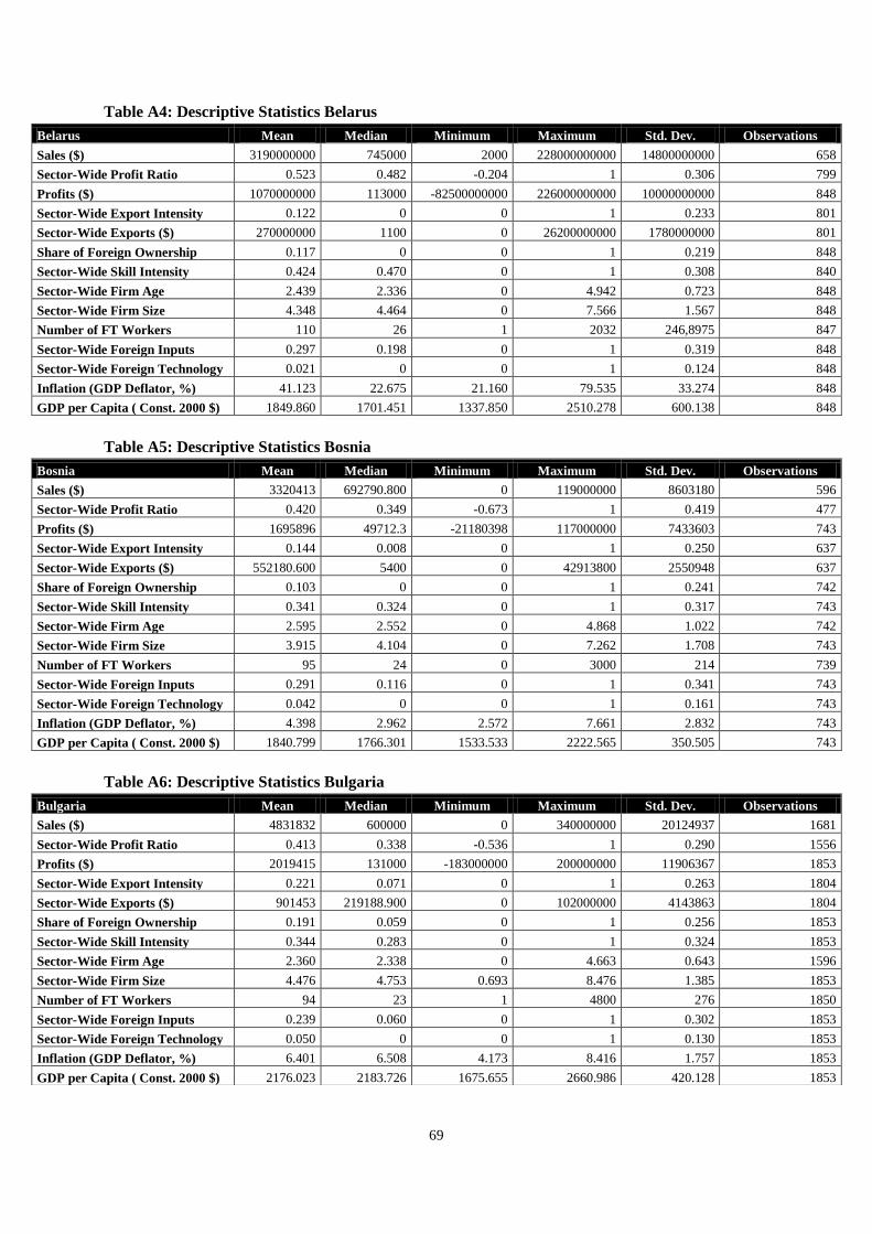
69

Table A4: Descriptive Statistics Belarus

Table A5: Descriptive Statistics Bosnia

Table A6: Descriptive Statistics Bulgaria

Belarus Mean Median Minimum Maximum Std. Dev. Observations

Sales ($) 3190000000 745000 2000 228000000000 14800000000 658

Sector-Wide Profit Ratio 0.523 0.482 -0.204 1 0.306 799

Profits ($) 1070000000 113000 -82500000000 226000000000 10000000000 848

Sector-Wide Export Intensity 0.122 0 0 1 0.233 801

Sector-Wide Exports ($) 270000000 1100 0 26200000000 1780000000 801

Share of Foreign Ownership 0.117 0 0 1 0.219 848

Sector-Wide Skill Intensity 0.424 0.470 0 1 0.308 840

Sector-Wide Firm Age 2.439 2.336 0 4.942 0.723 848

Sector-Wide Firm Size 4.348 4.464 0 7.566 1.567 848

Number of FT Workers 110 26 1 2032 246,8975 847

Sector-Wide Foreign Inputs 0.297 0.198 0 1 0.319 848

Sector-Wide Foreign Technology 0.021 0 0 1 0.124 848

Inflation (GDP Deflator, %) 41.123 22.675 21.160 79.535 33.274 848

GDP per Capita ( Const. 2000 $) 1849.860 1701.451 1337.850 2510.278 600.138 848

Bosnia Mean Median Minimum Maximum Std. Dev. Observations

Sales ($) 3320413 692790.800 0 119000000 8603180 596

Sector-Wide Profit Ratio 0.420 0.349 -0.673 1 0.419 477

Profits ($) 1695896 49712.3 -21180398 117000000 7433603 743

Sector-Wide Export Intensity 0.144 0.008 0 1 0.250 637

Sector-Wide Exports ($) 552180.600 5400 0 42913800 2550948 637

Share of Foreign Ownership 0.103 0 0 1 0.241 742

Sector-Wide Skill Intensity 0.341 0.324 0 1 0.317 743

Sector-Wide Firm Age 2.595 2.552 0 4.868 1.022 742

Sector-Wide Firm Size 3.915 4.104 0 7.262 1.708 743

Number of FT Workers 95 24 0 3000 214 739

Sector-Wide Foreign Inputs 0.291 0.116 0 1 0.341 743

Sector-Wide Foreign Technology 0.042 0 0 1 0.161 743

Inflation (GDP Deflator, %) 4.398 2.962 2.572 7.661 2.832 743

GDP per Capita ( Const. 2000 $) 1840.799 1766.301 1533.533 2222.565 350.505 743

Bulgaria Mean Median Minimum Maximum Std. Dev. Observations

Sales ($) 4831832 600000 0 340000000 20124937 1681

Sector-Wide Profit Ratio 0.413 0.338 -0.536 1 0.290 1556

Profits ($) 2019415 131000 -183000000 200000000 11906367 1853

Sector-Wide Export Intensity 0.221 0.071 0 1 0.263 1804

Sector-Wide Exports ($) 901453 219188.900 0 102000000 4143863 1804

Share of Foreign Ownership 0.191 0.059 0 1 0.256 1853

Sector-Wide Skill Intensity 0.344 0.283 0 1 0.324 1853

Sector-Wide Firm Age 2.360 2.338 0 4.663 0.643 1596

Sector-Wide Firm Size 4.476 4.753 0.693 8.476 1.385 1853

Number of FT Workers 94 23 1 4800 276 1850

Sector-Wide Foreign Inputs 0.239 0.060 0 1 0.302 1853

Sector-Wide Foreign Technology 0.050 0 0 1 0.130 1853

Inflation (GDP Deflator, %) 6.401 6.508 4.173 8.416 1.757 1853

GDP per Capita ( Const. 2000 $) 2176.023 2183.726 1675.655 2660.986 420.128 1853

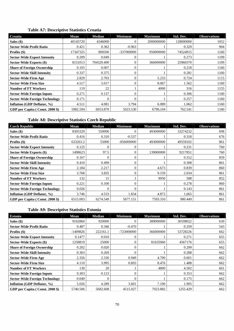
70

Table A7: Descriptive Statistics Croatia

Table A8: Descriptive Statistics Czech Republic

Table A9: Descriptive Statistics Estonia

Croatia Mean Median Minimum Maximum Std. Dev. Observations

Sales ($) 40145720 4346000 0 2000000000 128000000 1052

Sector-Wide Profit Ratio 0.421 0.362 -0.963 1 0.329 904

Profits ($) 17347325 800500 -337000000 950000000 74524915 1160

Sector-Wide Export Intensity 0.209 0.049 0 1 0.273 1109

Sector-Wide Exports ($) 8151013 704329.400 0 366000000 25960370 1109

Share of Foreign Ownership 0.105 0.007 0 1 0.218 1160

Sector-Wide Skill Intensity 0.337 0.375 0 1 0.281 1160

Sector-Wide Firm Age 2.829 2.703 0 5.233 0.724 1115

Sector-Wide Firm Size 4.517 5.017 0 8.067 1.562 1160

Number of FT Workers 119 22 1 4000 316 1155

Sector-Wide Foreign Inputs 0.271 0.137 0 1 0.306 1160

Sector-Wide Foreign Technology 0.171 0 0 1 0.257 1160

Inflation (GDP Deflator, %) 4.511 4.081 3.794 6.089 1.062 1160

GDP per Capita ( Const. 2000 $) 5982.594 6053.870 5023.530 6799,104 762.541 1160

Czech Republic Mean Median Minimum Maximum Std. Dev. Observations

Sales ($) 8305329 550000 0 493000000 33274232 698

Sector-Wide Profit Ratio 0.416 0.310 -0.537 1 0.318 676

Profits ($) 633263.2 55000 -856000000 493000000 49559102 861

Sector-Wide Export Intensity 0.125 0 0 1 0.231 760

Sector-Wide Exports ($) 1498623 97.5 0 139000000 9217851 760

Share of Foreign Ownership 0.167 0 0 1 0.312 859

Sector-Wide Skill Intensity 0.410 0.499 0 1 0.308 861

Sector-Wide Firm Age 2.184 2.217 0 4.673 0.839 860

Sector-Wide Firm Size 3.768 3.835 0 9.159 2.034 861

Number of FT Workers 132 15 1 9950 588 852

Sector-Wide Foreign Inputs 0.221 0.100 0 1 0.278 860

Sector-Wide Foreign Technology 0.026 0 0 1 0.143 861

Inflation (GDP Deflator, %) 3.746 4.533 1.834 4.872 1,665 861

GDP per Capita ( Const. 2000 $) 6515.003 6274.549 5677.151 7593.310 980.449 861

Estonia Mean Median Minimum Maximum Std. Dev. Observations

Sales ($) 9162860 920000 0 389000000 30108022 639

Sector-Wide Profit Ratio 0.487 0.346 -0.470 1 0.359 543

Profits ($) -1409826 222161.1 -723000000 366000000 53728226 662

Sector-Wide Export Intensity 0.1477 0.010 0 1 0.271 655

Sector-Wide Exports ($) 1258819 25000 0 81635960 4567176 655

Share of Foreign Ownership 0.202 0.020 0 1 0.299 662

Sector-Wide Skill Intensity 0.303 0.269 0 1 0.288 662

Sector-Wide Firm Age 2.356 2.336 0.949 4.700 0.601 662

Sector-Wide Firm Size 4.110 3.995 0.693 8.476 1.488 662

Number of FT Workers 130 20 1 4800 4.502 661

Sector-Wide Foreign Inputs 0.303 0.123 0 1 0.353 662

Sector-Wide Foreign Technology 0.049 0 0 1 0.175 662

Inflation (GDP Deflator, %) 5.026 4.289 3.601 7.190 1.905 662

GDP per Capita ( Const. 2000 $) 5740.506 5682.608 4515.027 7023.882 1255.429 662

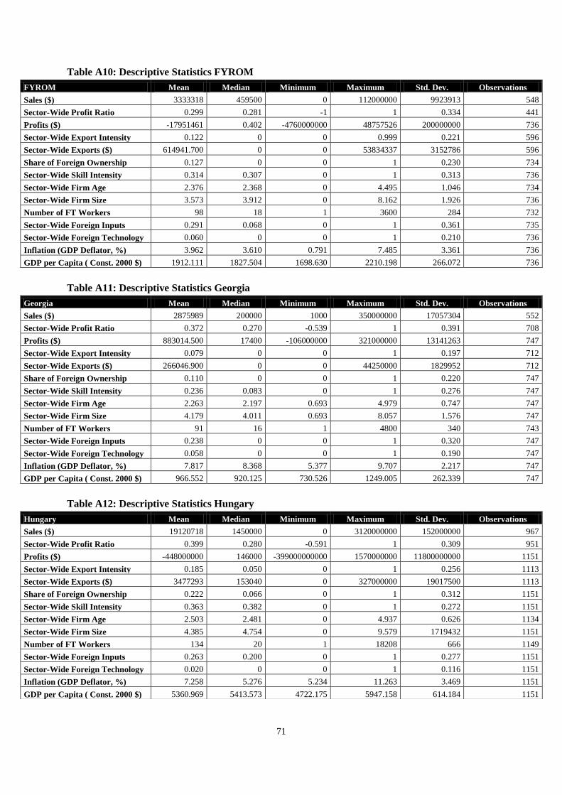
71

Table A10: Descriptive Statistics FYROM

Table A11: Descriptive Statistics Georgia

Table A12: Descriptive Statistics Hungary

FYROM Mean Median Minimum Maximum Std. Dev. Observations

Sales ($) 3333318 459500 0 112000000 9923913 548

Sector-Wide Profit Ratio 0.299 0.281 -1 1 0.334 441

Profits ($) -17951461 0.402 -4760000000 48757526 200000000 736

Sector-Wide Export Intensity 0.122 0 0 0.999 0.221 596

Sector-Wide Exports ($) 614941.700 0 0 53834337 3152786 596

Share of Foreign Ownership 0.127 0 0 1 0.230 734

Sector-Wide Skill Intensity 0.314 0.307 0 1 0.313 736

Sector-Wide Firm Age 2.376 2.368 0 4.495 1.046 734

Sector-Wide Firm Size 3.573 3.912 0 8.162 1.926 736

Number of FT Workers 98 18 1 3600 284 732

Sector-Wide Foreign Inputs 0.291 0.068 0 1 0.361 735

Sector-Wide Foreign Technology 0.060 0 0 1 0.210 736

Inflation (GDP Deflator, %) 3.962 3.610 0.791 7.485 3.361 736

GDP per Capita ( Const. 2000 $) 1912.111 1827.504 1698.630 2210.198 266.072 736

Georgia Mean Median Minimum Maximum Std. Dev. Observations

Sales ($) 2875989 200000 1000 350000000 17057304 552

Sector-Wide Profit Ratio 0.372 0.270 -0.539 1 0.391 708

Profits ($) 883014.500 17400 -106000000 321000000 13141263 747

Sector-Wide Export Intensity 0.079 0 0 1 0.197 712

Sector-Wide Exports ($) 266046.900 0 0 44250000 1829952 712

Share of Foreign Ownership 0.110 0 0 1 0.220 747

Sector-Wide Skill Intensity 0.236 0.083 0 1 0.276 747

Sector-Wide Firm Age 2.263 2.197 0.693 4.979 0.747 747

Sector-Wide Firm Size 4.179 4.011 0.693 8.057 1.576 747

Number of FT Workers 91 16 1 4800 340 743

Sector-Wide Foreign Inputs 0.238 0 0 1 0.320 747

Sector-Wide Foreign Technology 0.058 0 0 1 0.190 747

Inflation (GDP Deflator, %) 7.817 8.368 5.377 9.707 2.217 747

GDP per Capita ( Const. 2000 $) 966.552 920.125 730.526 1249.005 262.339 747

Hungary Mean Median Minimum Maximum Std. Dev. Observations

Sales ($) 19120718 1450000 0 3120000000 152000000 967

Sector-Wide Profit Ratio 0.399 0.280 -0.591 1 0.309 951

Profits ($) -448000000 146000 -399000000000 1570000000 11800000000 1151

Sector-Wide Export Intensity 0.185 0.050 0 1 0.256 1113

Sector-Wide Exports ($) 3477293 153040 0 327000000 19017500 1113

Share of Foreign Ownership 0.222 0.066 0 1 0.312 1151

Sector-Wide Skill Intensity 0.363 0.382 0 1 0.272 1151

Sector-Wide Firm Age 2.503 2.481 0 4.937 0.626 1134

Sector-Wide Firm Size 4.385 4.754 0 9.579 1719432 1151

Number of FT Workers 134 20 1 18208 666 1149

Sector-Wide Foreign Inputs 0.263 0.200 0 1 0.277 1151

Sector-Wide Foreign Technology 0.020 0 0 1 0.116 1151

Inflation (GDP Deflator, %) 7.258 5.276 5.234 11.263 3.469 1151

GDP per Capita ( Const. 2000 $) 5360.969 5413.573 4722.175 5947.158 614.184 1151

72

Table A13: Descriptive Statistics Kazakhstan

Table A14: Descriptive Statistics Kyrgyz

Table A15: Descriptive Statistics Latvia

Kazakhstan Mean Median Minimum Maximum Std. Dev. Observations

Sales ($) 2138164 184500 0 147000000 8232560 1166

Sector-Wide Profit Ratio 0.324 0.231 -0.942 1 0.320 908

Profits ($) -31501003 11000 -7930000000 139000000 303000000 1379

Sector-Wide Export Intensity 0.043 0 0 0.990 0.108 1345

Sector-Wide Exports ($) 99377.100 0 0 13642947 611356.8 1345

Share of Foreign Ownership 0.074 0.007 0 1 0.172 1379

Sector-Wide Skill Intensity 0.370 0.458 0 0.958 0.277 1379

Sector-Wide Firm Age 2.097 2.144 0 4.595 0.522 1332

Sector-Wide Firm Size 4.676 4.745 0 9.190 1.277 1379

Number of FT Workers 109 30 2 9800 369 1375

Sector-Wide Foreign Inputs 0.224 0.120 0 1 0.266 1379

Sector-Wide Foreign Technology 0.027 0 0 1 0.129 1379

Inflation (GDP Deflator, %) 15.742 16.132 10.156 20.937 5.401 1379

GDP per Capita ( Const. 2000 $) 1865.445 1818.959 1397.290 2380.085 493.044 1379

Kyrgyz Mean Median Minimum Maximum Std. Dev. Observations

Sales ($) 715779 92453 0 42474785 2751874 506

Sector-Wide Profit Ratio 0.449 0.360 -0.906 1 0.348 413

Profits ($) -7552606 11000 -1250000000 28718786 87276594 610

Sector-Wide Export Intensity 0.091 0 0 1 0.221 572

Sector-Wide Exports ($) 125079.500 0 0 19147250 1007057 572

Share of Foreign Ownership 0.118 0 0 1 0.231 609

Sector-Wide Skill Intensity 0.341 0.347 0 0.900 0.277 610

Sector-Wide Firm Age 2.393 2.291 0 4.715 0.773 605

Sector-Wide Firm Size 3.856 3.869 0 7.754 1.339 610

Number of FT Workers 84 24 1 2331 2.019 608

Sector-Wide Foreign Inputs 0.280 0.119 0 1 0.339 609

Sector-Wide Foreign Technology 0.048 0 0 1 0.181 610

Inflation (GDP Deflator, %) 11.552 7.332 5.108 22.216 9.302 610

GDP per Capita ( Const. 2000 $) 330.527 323.670 291.725 376.187 42.646 610

Latvia Mean Median Minimum Maximum Std. Dev. Observations

Sales ($) 9223165 609500 0 773000000 47495023 604

Sector-Wide Profit Ratio 0.507 0.513 -0.937 1 0.364 555

Profits ($) 4866722 212830 -57528000 376000000 2.577 652

Sector-Wide Export Intensity 0.127 0 0 1 0.266 639

Sector-Wide Exports ($) 897640.600 0 0 24800643 3.141 639

Share of Foreign Ownership 0.236 0 0 1 0.326 652

Sector-Wide Skill Intensity 0.317 0.294 0 1 0.289 652

Sector-Wide Firm Age 2.228 2.262 0 4.803 0.677 652

Sector-Wide Firm Size 4.232 4.657 0 8.441 1.909 652

Number of FT Workers 127 18 1 6697 469 648

Sector-Wide Foreign Inputs 0.328 0.193 0 1 0.353 652

Sector-Wide Foreign Technology 0.051 0 0 1 0.191 652

Inflation (GDP Deflator, %) 7.696 7.009 1.695 14.383 6.372 652

GDP per Capita ( Const. 2000 $) 4729.393 4538.848 3593.665 6055.665 1242.011 652

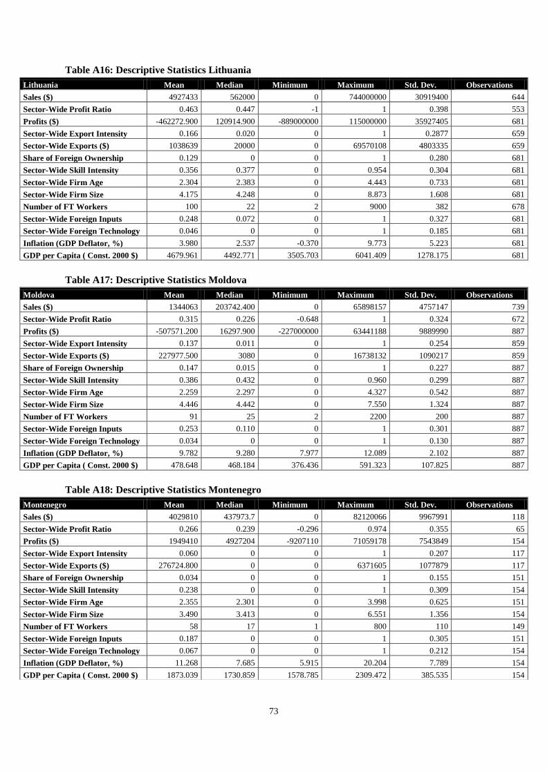
73

Table A16: Descriptive Statistics Lithuania

Table A17: Descriptive Statistics Moldova

Table A18: Descriptive Statistics Montenegro

Lithuania Mean Median Minimum Maximum Std. Dev. Observations

Sales ($) 4927433 562000 0 744000000 30919400 644

Sector-Wide Profit Ratio 0.463 0.447 -1 1 0.398 553

Profits ($) -462272.900 120914.900 -889000000 115000000 35927405 681

Sector-Wide Export Intensity 0.166 0.020 0 1 0.2877 659

Sector-Wide Exports ($) 1038639 20000 0 69570108 4803335 659

Share of Foreign Ownership 0.129 0 0 1 0.280 681

Sector-Wide Skill Intensity 0.356 0.377 0 0.954 0.304 681

Sector-Wide Firm Age 2.304 2.383 0 4.443 0.733 681

Sector-Wide Firm Size 4.175 4.248 0 8.873 1.608 681

Number of FT Workers 100 22 2 9000 382 678

Sector-Wide Foreign Inputs 0.248 0.072 0 1 0.327 681

Sector-Wide Foreign Technology 0.046 0 0 1 0.185 681

Inflation (GDP Deflator, %) 3.980 2.537 -0.370 9.773 5.223 681

GDP per Capita ( Const. 2000 $) 4679.961 4492.771 3505.703 6041.409 1278.175 681

Moldova Mean Median Minimum Maximum Std. Dev. Observations

Sales ($) 1344063 203742.400 0 65898157 4757147 739

Sector-Wide Profit Ratio 0.315 0.226 -0.648 1 0.324 672

Profits ($) -507571.200 16297.900 -227000000 63441188 9889990 887

Sector-Wide Export Intensity 0.137 0.011 0 1 0.254 859

Sector-Wide Exports ($) 227977.500 3080 0 16738132 1090217 859

Share of Foreign Ownership 0.147 0.015 0 1 0.227 887

Sector-Wide Skill Intensity 0.386 0.432 0 0.960 0.299 887

Sector-Wide Firm Age 2.259 2.297 0 4.327 0.542 887

Sector-Wide Firm Size 4.446 4.442 0 7.550 1.324 887

Number of FT Workers 91 25 2 2200 200 887

Sector-Wide Foreign Inputs 0.253 0.110 0 1 0.301 887

Sector-Wide Foreign Technology 0.034 0 0 1 0.130 887

Inflation (GDP Deflator, %) 9.782 9.280 7.977 12.089 2.102 887

GDP per Capita ( Const. 2000 $) 478.648 468.184 376.436 591.323 107.825 887

Montenegro Mean Median Minimum Maximum Std. Dev. Observations

Sales ($) 4029810 437973.7 0 82120066 9967991 118

Sector-Wide Profit Ratio 0.266 0.239 -0.296 0.974 0.355 65

Profits ($) 1949410 4927204 -9207110 71059178 7543849 154

Sector-Wide Export Intensity 0.060 0 0 1 0.207 117

Sector-Wide Exports ($) 276724.800 0 0 6371605 1077879 117

Share of Foreign Ownership 0.034 0 0 1 0.155 151

Sector-Wide Skill Intensity 0.238 0 0 1 0.309 154

Sector-Wide Firm Age 2.355 2.301 0 3.998 0.625 151

Sector-Wide Firm Size 3.490 3.413 0 6.551 1.356 154

Number of FT Workers 58 17 1 800 110 149

Sector-Wide Foreign Inputs 0.187 0 0 1 0.305 151

Sector-Wide Foreign Technology 0.067 0 0 1 0.212 154

Inflation (GDP Deflator, %) 11.268 7.685 5.915 20.204 7.789 154

GDP per Capita ( Const. 2000 $) 1873.039 1730.859 1578.785 2309.472 385.535 154

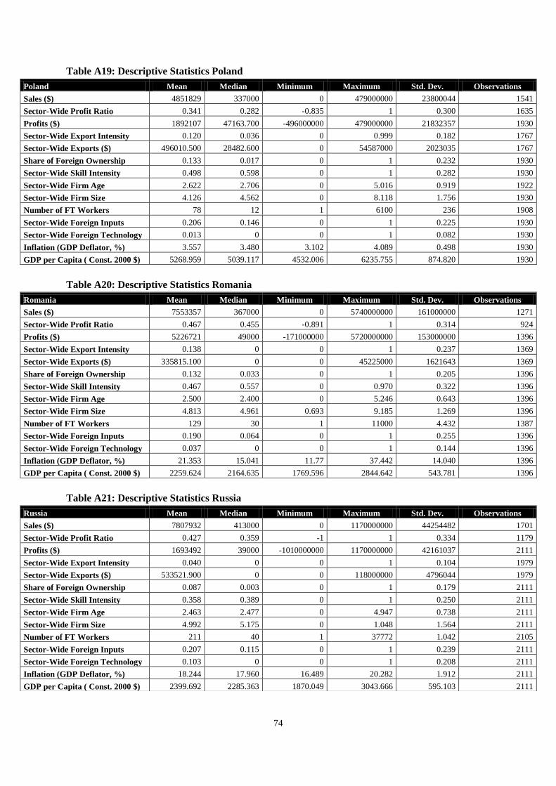
74

Table A19: Descriptive Statistics Poland

Table A20: Descriptive Statistics Romania

Table A21: Descriptive Statistics Russia

Poland Mean Median Minimum Maximum Std. Dev. Observations

Sales ($) 4851829 337000 0 479000000 23800044 1541

Sector-Wide Profit Ratio 0.341 0.282 -0.835 1 0.300 1635

Profits ($) 1892107 47163.700 -496000000 479000000 21832357 1930

Sector-Wide Export Intensity 0.120 0.036 0 0.999 0.182 1767

Sector-Wide Exports ($) 496010.500 28482.600 0 54587000 2023035 1767

Share of Foreign Ownership 0.133 0.017 0 1 0.232 1930

Sector-Wide Skill Intensity 0.498 0.598 0 1 0.282 1930

Sector-Wide Firm Age 2.622 2.706 0 5.016 0.919 1922

Sector-Wide Firm Size 4.126 4.562 0 8.118 1.756 1930

Number of FT Workers 78 12 1 6100 236 1908

Sector-Wide Foreign Inputs 0.206 0.146 0 1 0.225 1930

Sector-Wide Foreign Technology 0.013 0 0 1 0.082 1930

Inflation (GDP Deflator, %) 3.557 3.480 3.102 4.089 0.498 1930

GDP per Capita ( Const. 2000 $) 5268.959 5039.117 4532.006 6235.755 874.820 1930

Romania Mean Median Minimum Maximum Std. Dev. Observations

Sales ($) 7553357 367000 0 5740000000 161000000 1271

Sector-Wide Profit Ratio 0.467 0.455 -0.891 1 0.314 924

Profits ($) 5226721 49000 -171000000 5720000000 153000000 1396

Sector-Wide Export Intensity 0.138 0 0 1 0.237 1369

Sector-Wide Exports ($) 335815.100 0 0 45225000 1621643 1369

Share of Foreign Ownership 0.132 0.033 0 1 0.205 1396

Sector-Wide Skill Intensity 0.467 0.557 0 0.970 0.322 1396

Sector-Wide Firm Age 2.500 2.400 0 5.246 0.643 1396

Sector-Wide Firm Size 4.813 4.961 0.693 9.185 1.269 1396

Number of FT Workers 129 30 1 11000 4.432 1387

Sector-Wide Foreign Inputs 0.190 0.064 0 1 0.255 1396

Sector-Wide Foreign Technology 0.037 0 0 1 0.144 1396

Inflation (GDP Deflator, %) 21.353 15.041 11.77 37.442 14.040 1396

GDP per Capita ( Const. 2000 $) 2259.624 2164.635 1769.596 2844.642 543.781 1396

Russia Mean Median Minimum Maximum Std. Dev. Observations

Sales ($) 7807932 413000 0 1170000000 44254482 1701

Sector-Wide Profit Ratio 0.427 0.359 -1 1 0.334 1179

Profits ($) 1693492 39000 -1010000000 1170000000 42161037 2111

Sector-Wide Export Intensity 0.040 0 0 1 0.104 1979

Sector-Wide Exports ($) 533521.900 0 0 118000000 4796044 1979

Share of Foreign Ownership 0.087 0.003 0 1 0.179 2111

Sector-Wide Skill Intensity 0.358 0.389 0 1 0.250 2111

Sector-Wide Firm Age 2.463 2.477 0 4.947 0.738 2111

Sector-Wide Firm Size 4.992 5.175 0 1.048 1.564 2111

Number of FT Workers 211 40 1 37772 1.042 2105

Sector-Wide Foreign Inputs 0.207 0.115 0 1 0.239 2111

Sector-Wide Foreign Technology 0.103 0 0 1 0.208 2111

Inflation (GDP Deflator, %) 18.244 17.960 16.489 20.282 1.912 2111

GDP per Capita ( Const. 2000 $) 2399.692 2285.363 1870.049 3043.666 595.103 2111

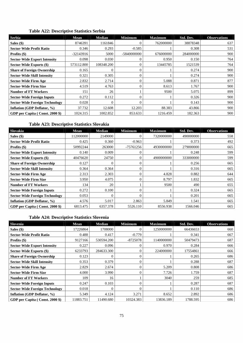
75

Table A22: Descriptive Statistics Serbia

Table A23: Descriptive Statistics Slovakia

Table A24: Descriptive Statistics Slovenia

Serbia Mean Median Minimum Maximum Std. Dev. Observations

Sales ($) 8746391 1161846 0 762000000 38878348 637

Sector-Wide Profit Ratio 0.346 0.293 -0.585 1 0.308 531

Profits ($) -32143916 5000 -5840000000 676000000 284000000 900

Sector-Wide Export Intensity 0.098 0.030 0 0.950 0.150 764

Sector-Wide Exports ($) 573112.800 108348.200 0 13445785 1521539 764

Share of Foreign Ownership 0.165 0 0 1 0.274 900

Sector-Wide Skill Intensity 0.321 0.305 0 1 0.274 900

Sector-Wide Firm Age 2.832 2.714 0 5.088 0.871 877

Sector-Wide Firm Size 4.519 4.763 0 8.613 1.767 900

Number of FT Workers 151 26 1 9500 5.075 899

Sector-Wide Foreign Inputs 0.272 0.112 0 1 0.326 900

Sector-Wide Foreign Technology 0.028 0 0 1 0.143 900

Inflation (GDP Deflator, %) 37.732 12.608 12.203 88.383 43.866 900

GDP per Capita ( Const. 2000 $) 1024.315 1002.852 853.633 1216.459 182.363 900

Slovakia Mean Median Minimum Maximum Std. Dev. Observations

Sales ($) 112000000 2149000 0 7320000000 490000000 558

Sector-Wide Profit Ratio 0.425 0.360 -0.963 1 0.373 492

Profits ($) 50992244 263000 -75761256 4930000000 279000000 665

Sector-Wide Export Intensity 0.140 0.009 0 1 0.248 599

Sector-Wide Exports ($) 40476620 24750 0 4900000000 333000000 599

Share of Foreign Ownership 0.127 0 0 1 0.256 665

Sector-Wide Skill Intensity 0.364 0.364 0 1 0.316 665

Sector-Wide Firm Age 2.313 2.303 0 4.828 0.882 644

Sector-Wide Firm Size 3.950 4.075 0 8.797 1.832 665

Number of FT Workers 134 20 1 9500 490 655

Sector-Wide Foreign Inputs 0.272 0.100 0 1 0.324 665

Sector-Wide Foreign Technology 0.053 0 0 1 0.201 665

Inflation (GDP Deflator, %) 4.576 5.017 2.863 5.849 1.541 665

GDP per Capita ( Const. 2000 $) 6813.475 6357.378 5526.110 8556.938 1566.046 665

Slovenia Mean Median Minimum Maximum Std. Dev. Observations

Sales ($) 17226864 1708000 0 1250000000 66436653 660

Sector-Wide Profit Ratio 0.488 0.417 -0.779 1 0.341 667

Profits ($) 9127166 530594.200 -8725078 1140000000 50479473 687

Sector-Wide Export Intensity 0.227 0.096 0 0.970 0.284 666

Sector-Wide Exports ($) 6233793 284633.300 0 224000000 17554861 666

Share of Foreign Ownership 0.123 0 0 1 0.265 686

Sector-Wide Skill Intensity 0.353 0.379 0 1 0.288 687

Sector-Wide Firm Age 2.829 2.674 0 5.209 0.808 686

Sector-Wide Firm Size 4.000 3.990 0 7.726 1.759 687

Number of FT Workers 109 16 1 3040 259 685

Sector-Wide Foreign Inputs 0.247 0.103 0 1 0.287 687

Sector-Wide Foreign Technology 0.018 0 0 1 0.110 686

Inflation (GDP Deflator, %) 5.349 4.124 3.271 8.652 2.892 686

GDP per Capita ( Const. 2000 $) 11883.751 11490.680 10324.383 13836.189 1788.595 686

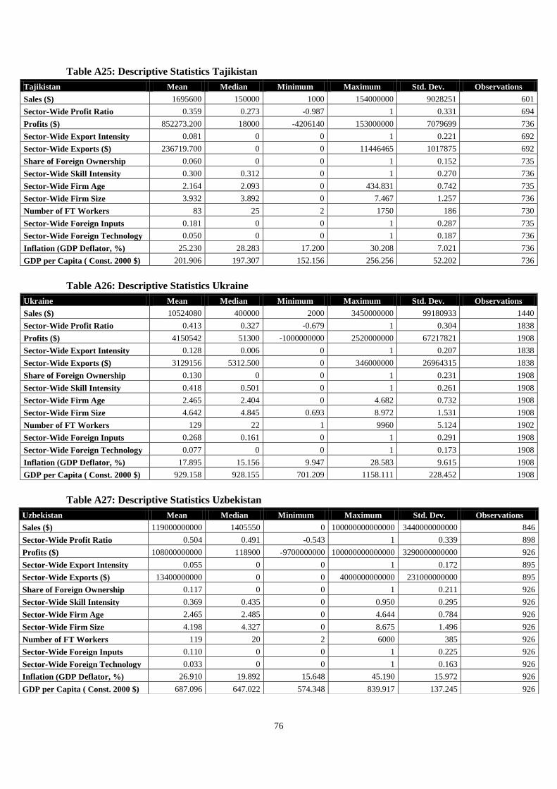
76

Table A25: Descriptive Statistics Tajikistan

Table A26: Descriptive Statistics Ukraine

Table A27: Descriptive Statistics Uzbekistan

Tajikistan Mean Median Minimum Maximum Std. Dev. Observations

Sales ($) 1695600 150000 1000 154000000 9028251 601

Sector-Wide Profit Ratio 0.359 0.273 -0.987 1 0.331 694

Profits ($) 852273.200 18000 -4206140 153000000 7079699 736

Sector-Wide Export Intensity 0.081 0 0 1 0.221 692

Sector-Wide Exports ($) 236719.700 0 0 11446465 1017875 692

Share of Foreign Ownership 0.060 0 0 1 0.152 735

Sector-Wide Skill Intensity 0.300 0.312 0 1 0.270 736

Sector-Wide Firm Age 2.164 2.093 0 434.831 0.742 735

Sector-Wide Firm Size 3.932 3.892 0 7.467 1.257 736

Number of FT Workers 83 25 2 1750 186 730

Sector-Wide Foreign Inputs 0.181 0 0 1 0.287 735

Sector-Wide Foreign Technology 0.050 0 0 1 0.187 736

Inflation (GDP Deflator, %) 25.230 28.283 17.200 30.208 7.021 736

GDP per Capita ( Const. 2000 $) 201.906 197.307 152.156 256.256 52.202 736

Ukraine Mean Median Minimum Maximum Std. Dev. Observations

Sales ($) 10524080 400000 2000 3450000000 99180933 1440

Sector-Wide Profit Ratio 0.413 0.327 -0.679 1 0.304 1838

Profits ($) 4150542 51300 -1000000000 2520000000 67217821 1908

Sector-Wide Export Intensity 0.128 0.006 0 1 0.207 1838

Sector-Wide Exports ($) 3129156 5312.500 0 346000000 26964315 1838

Share of Foreign Ownership 0.130 0 0 1 0.231 1908

Sector-Wide Skill Intensity 0.418 0.501 0 1 0.261 1908

Sector-Wide Firm Age 2.465 2.404 0 4.682 0.732 1908

Sector-Wide Firm Size 4.642 4.845 0.693 8.972 1.531 1908

Number of FT Workers 129 22 1 9960 5.124 1902

Sector-Wide Foreign Inputs 0.268 0.161 0 1 0.291 1908

Sector-Wide Foreign Technology 0.077 0 0 1 0.173 1908

Inflation (GDP Deflator, %) 17.895 15.156 9.947 28.583 9.615 1908

GDP per Capita ( Const. 2000 $) 929.158 928.155 701.209 1158.111 228.452 1908

Uzbekistan Mean Median Minimum Maximum Std. Dev. Observations

Sales ($) 119000000000 1405550 0 100000000000000 3440000000000 846

Sector-Wide Profit Ratio 0.504 0.491 -0.543 1 0.339 898

Profits ($) 108000000000 118900 -9700000000 100000000000000 3290000000000 926

Sector-Wide Export Intensity 0.055 0 0 1 0.172 895

Sector-Wide Exports ($) 13400000000 0 0 4000000000000 231000000000 895

Share of Foreign Ownership 0.117 0 0 1 0.211 926

Sector-Wide Skill Intensity 0.369 0.435 0 0.950 0.295 926

Sector-Wide Firm Age 2.465 2.485 0 4.644 0.784 926

Sector-Wide Firm Size 4.198 4.327 0 8.675 1.496 926

Number of FT Workers 119 20 2 6000 385 926

Sector-Wide Foreign Inputs 0.110 0 0 1 0.225 926

Sector-Wide Foreign Technology 0.033 0 0 1 0.163 926

Inflation (GDP Deflator, %) 26.910 19.892 15.648 45.190 15.972 926

GDP per Capita ( Const. 2000 $) 687.096 647.022 574.348 839.917 137.245 926

77