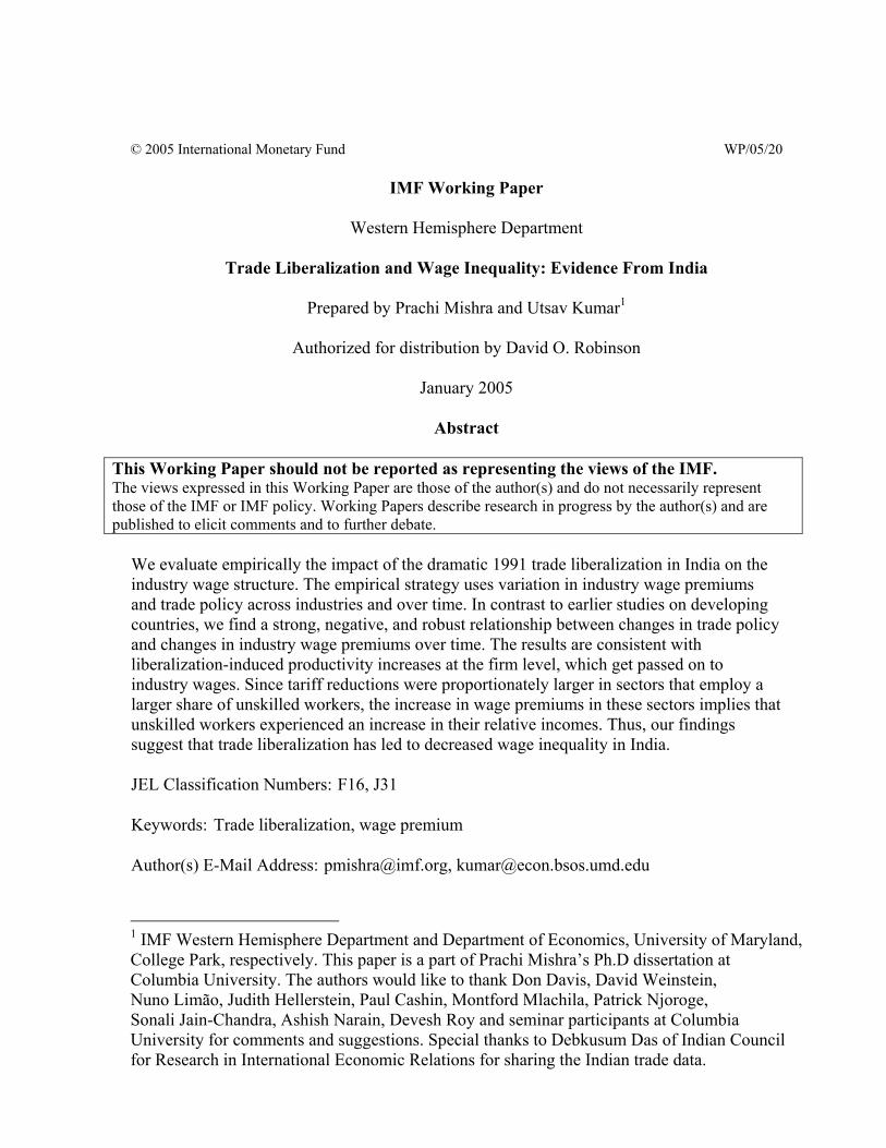
WP/05/20

Trade Liberalization and Wage Inequality: Evidence From India

Prachi Mishra and Utsav Kumar

© 2005 International Monetary Fund WP/05/20

IMF Working Paper

Western Hemisphere Department

Trade Liberalization and Wage Inequality: Evidence From India

Prepared by Prachi Mishra and Utsav Kumar1

Authorized for distribution by David O. Robinson

January 2005

Abstract

This Working Paper should not be reported as representing the views of the IMF. The views expressed in this Working Paper are those of the author(s) and do not necessarily represent those of the IMF or IMF policy. Working Papers describe research in progress by the author(s) and are published to elicit comments and to further debate.

We evaluate empirically the impact of the dramatic 1991 trade liberalization in India on the industry wage structure. The empirical strategy uses variation in industry wage premiums and trade policy across industries and over time. In contrast to earlier studies on developing countries, we find a strong, negative, and robust relationship between changes in trade policy and changes in industry wage premiums over time. The results are consistent with liberalization-induced productivity increases at the firm level, which get passed on to industry wages. Since tariff reductions were proportionately larger in sectors that employ a larger share of unskilled workers, the increase in wage premiums in these sectors implies that unskilled workers experienced an increase in their relative incomes. Thus, our findings suggest that trade liberalization has led to decreased wage inequality in India. JEL Classification Numbers: F16, J31 Keywords: Trade liberalization, wage premium Author(s) E-Mail Address: pmishra@imf.org, kumar@econ.bsos.umd.edu

1 IMF Western Hemisphere Department and Department of Economics, University of Maryland, College Park, respectively. This paper is a part of Prachi Mishra’s Ph.D dissertation at Columbia University. The authors would like to thank Don Davis, David Weinstein, Nuno Limão, Judith Hellerstein, Paul Cashin, Montford Mlachila, Patrick Njoroge, Sonali Jain-Chandra, Ashish Narain, Devesh Roy and seminar participants at Columbia University for comments and suggestions. Special thanks to Debkusum Das of Indian Council for Research in International Economic Relations for sharing the Indian trade data.

- 2 -

Contents Page I. Introduction.......................................................................................................................4 II. Background of India’s Trade Liberalization.....................................................................5 III. Predictions of the Theoretical Models ..............................................................................6 IV. Empirical Strategy ............................................................................................................7 V. Data Description ...............................................................................................................8 A. Trade Policy in India................................................................................................8 B. National Sample Survey Data..................................................................................9 VI. Results.............................................................................................................................10 A. Estimation of Interindustry Wage Premiums.........................................................10 B. Why Do Industry Wage Premiums Exist in India?................................................11

C. Industry Wage Premiums and Trade Policy ..........................................................13 D. Discussion of the Results .......................................................................................15 E. Endogeneity Issues.................................................................................................16 F. Additional Robustness Checks ..............................................................................18 VII. Conclusions.....................................................................................................................18 Tables 1. Correlations of Tariffs Over Time ..................................................................................20 2. Results from the Earnings Regression ............................................................................21 3. Correlation Matrix for Industry Wage Premiums...........................................................22 4. Tariffs and Industry Wage Premiums .............................................................................23 5. Tariffs and Industry Wage Premiums: Controlling for Nontrade Barriers and Import Penetration Ratios ...........................................................................................24 6A. Tariffs and Industry Wage Premiums: Instrumental Variable Regression .....................25 6B. First Stage Instrumental Variable Regression.................................................................26 7. Tariffs and Industry Wage premiums: Controlling for Gross Fixed Capital Formation ........................................................................................................27 Figures 1A. Average Tariff Rates in Manufacturing..........................................................................28 1B. Average Tariff Rates: India and Latin America .............................................................29 2. Tariffs: Pre and Post Liberalization ................................................................................30 3. Non-Tariff Barriers: Average Import Coverage Ratio....................................................31 4. Tariff Reduction and Pre-Liberalization Tariffs .............................................................32 5. Tariff Reduction and Share of Unskilled Workers .........................................................33 6. Tariff Reduction between 1983–84 and 1999–2000 and Industry Wage Premium in 1983−84 .........................................................................................34

- 3 -

7. Scatter Diagram Relating Differences in Wage Premiums and Differences in Tariffs...................................................................................................35 8. Foreign Exchange Reserves............................................................................................36 Annex Table 1. Estimated Industry Wage Premiums......................................................................37 Table 2. Correlations in Industry Wage Premiums by Occupations....................................40 References ................................................................................................................................41

- 4 -

I. INTRODUCTION

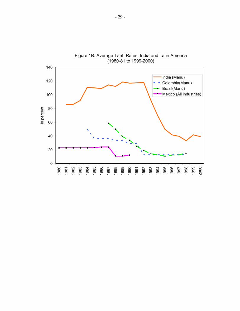
A growing body of research indicates that trade liberalization by developing countries has raised their aggregate incomes.2 Academic and policy debates on the merits and demerits of liberalization have centered on the internal distributional consequences and on the question of how trade reforms affect labor markets. This paper presents new evidence from India on the impact of trade liberalization on wages. India offers an excellent case to study the effects of trade liberalization for two reasons. First, the magnitude of trade liberalization in India was very big. In 1991, after decades of pursuing an import-substitution industrialization strategy, India initiated a drastic liberalization of its external sector. The average tariff in manufacturing declined from 117 percent in 1990–91 to 39 percent in 1999–2000. The reduction in tariffs was much more drastic in India than in the trade liberalization episodes in Latin American countries like Mexico, Colombia, and Brazil. In addition to tariffs, India also has reduced nontariff barriers (NTBs) since 1991. The average import coverage ratio (the share of imports subject to nontariff barriers) declined from 82 percent in 1990–91 to 17 percent in 1999–2000. In fact, the 1991 trade reform in India represented one of the most dramatic trade liberalizations ever attempted in a developing country (Aghion et al., 2003). Second, the trade reforms in India were exogenous and came as a surprise. In response to a severe balance of payments crisis in 1991, India approached the International Monetary Fund for assistance. The IMF support was conditional on structural reforms including trade liberalization, which India launched. The government’s objectives when reducing trade barriers were given by IMF conditionalities. From an industry perspective, the target tariff rates were exogenously predetermined and policymakers had less room to cater to special lobby interests. Hence, the Indian trade liberalization episode offers an excellent natural experiment to examine the causal impact of trade reforms on the labor market. We use a dataset that combines micro-level data from the National Sample Survey Organization (NSSO) with data on international trade protection for the years 1980–2000. The empirical strategy in this paper uses variation in industry wage premiums and trade policy across industries and over time. Industry wage premiums are defined as the portion of individual wages that accrues to the worker’s industry affiliation after controlling for worker characteristics. Since different industries employ different proportions of skilled workers, changes in wage premiums translate into changes in the relative incomes of skilled and unskilled workers (Blom et. al., 2004; Goldberg and Pavcnik, 2004).

2 For example, see Frankel and Romer (1999).

- 5 -

First, we analyze industry wage premiums in the manufacturing sector in India. The main finding is that large differences in wages across industries exist for seemingly similar workers. Also, the structure of industry wage differentials in India has changed over time. Labor market rigidities seem to be a plausible explanation for the existence of wage premiums in India. Next, we examine empirically the impact of trade liberalization on industry wage differentials. The existing studies on the relationship between trade policy and industry wage premiums in developing countries yield mixed conclusions (Goldberg and Pavcnik, 2004, Blom et al., 2004, Feliciano, 2001). These studies find a positive or a statistically insignificant relationship between changes in trade policy and changes in wage differentials over time. In contrast, we find a strong and negative relationship between changes in trade policy and changes in wage differentials. The negative relationship is robust to instrumenting for tariffs and to including measures of nontariff barriers. Since the tariff reductions were relatively larger in sectors with a higher proportion of unskilled workers, and these sectors experienced an increase in relative wages, the unskilled workers experienced an increase in incomes relative to skilled workers. Thus, the findings in this paper suggest that trade liberalization has led to decreased wage inequality in India. This paper is organized as follows. Section II presents the background of India’s trade liberalization, Section III gives the predictions of the theoretical models, Section IV presents the empirical strategy, Section V describes the data and the evidence, and Section VI discusses the results. Section VII concludes.

II. BACKGROUND OF INDIA’S TRADE LIBERALIZATION

Following independence from the British rule in 1947, India embarked on a socialist strategy of development, which envisaged a heavy role for the government and the public sector in shaping India’s economy and industrialization. The strategy relied on import-substitution, emphasized the role of the government in providing infrastructure, as a regulator, and as a provider of goods and services. Throughout the 1960s and 1970s, the growth rate of GDP in India had been stagnant at 3−3.5 percent per annum (what came to be known as the Hindu rate of growth). Beginning in the early 1980s, there was some emergence of thinking about the need for a change in trade policy (Das, 2003). During the 1980s, the limitations of inward oriented development strategy, import substitution based industrialization, extensive government control, and the license raj were becoming increasingly evident. The trade regime in the early 1980s was characterized by high nominal tariffs and nontariff barriers coupled with a complex import licensing system. In addition, India’s tariff structure was very complex with a myriad of exemptions applicable to the basic duty rate and this was one of the areas which the trade reforms initiated in 1991 dealt with.

- 6 -

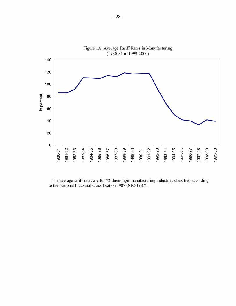
During the late 1980s, the then government took the first steps towards reducing state control. These were not only on the external policy front but also related to domestic industrial policy. Steps were taken to ease industrial and import licensing, replace quantitative restrictions with tariff barriers, simplify the tariff structure, and importantly, this was the first instance of a three-year trade policy. There were conscious efforts to dismantle the import licensing regime via reductions in the number of products listed under banned/restricted category (Das, 2003). However, these measures were too little and left a lot to be desired. Figures 1A and 2 show that till 1991, the levels of protection were very high―in 1991, the average tariff rate was 117 percent and the import coverage ratio was 82 percent. The years 1989–91 were marked by difficulties, both on the economic and political fronts. As the new government took over the treasury benches in 1991, India was facing an impending external payments crisis with foreign currency assets less than US$1 billion, just enough to cover two weeks of imports. The Government of India requested a Stand-By-Arrangement from the IMF in August 1991 and entered into an IMF-supported program. In addition to deficit reducing policies, a wide array of policies spanning the external, trade, industrial, public sector, financial and banking sectors were implemented. Some of the measures on the external front included elimination of the monopoly of state trading agencies, easing of import licensing, removing export restrictions, allowing foreign investment into the previously reserved sectors and full convertibility of domestic currency on foreign exchange transactions. The export-import policy (EXIM policy) of 1992–97 reaffirmed India’s commitment to freer trade. All import licensing lists were eliminated and a “negative” list was established. Except consumer goods, almost all capital and intermediate goods could be freely imported subject to tariffs. By April 2002, all the remaining quantitative restrictions were removed. Despite all the initial opposition to liberalization, reforms have been continued by every successive government.

III. PREDICTIONS OF THE THEORETICAL MODELS

In order to analyze the channels through which trade liberalization could affect industry wage differentials, it is important to look at the possible explanations as to why wage differentials exist in the first place. The labor literature on industry wage premiums in developed countries suggests several explanations for the existence of large wage differentials across industries for seemingly similar workers (Dickens and Katz (1987), Krueger and Summers (1988), Katz et al (1989)). The explanations offered by a standard competitive labor market model include differences in labor quality and/or compensating wage differentials for the quality of employment. Industry wage differences could also reflect transitory differentials related to imperfect short run labor mobility.

- 7 -

Noncompetitive explanations for the existence of industry wage differentials include efficiency wage theories, rent sharing by firms, or collective action threat and bargaining models. There has not been a consensus in the literature as to which theory explains the existence of industry wage premiums. “No single model appears entirely consistent with all the evidence on wage differences” (Dickens and Katz, 1987). Trade liberalization could affect industry wage premiums in perfectly competitive product and factor markets if there is short-run immobility of labor (specific factors model). In this case, trade liberalization would reduce the relative returns to the factor specific to the sector in which tariffs are reduced more. Trade liberalization could also affect wages in perfect competition models if workers are heterogeneous. Reduction in tariffs could affect relative wages by changing the composition of workers. However, if industry wage differentials exist due to compensating differentials, trade liberalization should not have any effect on wage premiums. Introducing imperfect competition in product and factor markets introduces additional channels through which trade liberalization can affect wage premiums. Trade liberalization could affect wage premiums by affecting capital or labor rents. It is also possible that unions extract part of the rents from protection in the form of more jobs rather than higher wages (McDonald and Solow, 1981). In this case, trade liberalization might not have any effect on relative wages but only affect employment. Grossman (1984) considers what happens when random layoff rules are replaced by seniority based layoff rules. Such a system induces senior workers to push for higher wages and junior workers to push for the low wages that prevent layoffs; the impact of trade liberalization then depends on the seniority structure of the union. Liberalization induced productivity changes at the firm level may also impact industry wages. Most empirical work has established a positive link between liberalization and productivity (e.g., Harrison, 1994, for Côte D’Ivoire; Krishna and Mitra, 1998, for India, Pavcnik, 2000, for Chile, etc.). The increased threat of foreign competition raises innovation incentives by domestic producers. To the extent that productivity enhancements are passed through onto industry wages, relative wages would be positively correlated with trade liberalization.

IV. EMPIRICAL STRATEGY

The strategy to estimate the impact of trade policy on wages follows the industry wage premium methodology. The methodology has been used extensively in the trade and labor literature (Krueger and Summers, 1988; Dickens and Katz, 1987; Gaston and Trefler, 1994; Goldberg and Pavcnik, 2004; Blom et al., 2004). The idea is to exploit variation in wages and tariffs (and other trade policy measures) across industries and over time to identify the impact of trade on wages.

- 8 -

The estimation has two stages. In the first stage, the log of individual worker (working in industry j and observed at time t ) i ’s wages ( )ln( ijtw ) are regressed on a vector of the worker’s characteristics ( ijtH ) like education, age, gender, geographical location, occupation, dummy for whether the worker is self employed, and a set of industry indicators ( ijtI ) reflecting the worker’s industry affiliation:

ijtjtijtHijtijt wpIHw εβ ++=)ln( (1) The coefficient on the industry dummy, the wage premium ( jtwp ), captures the part of the variation in wages that is explained by the worker’s industry affiliation. Following Krueger and Summers (1988), the estimated wage premiums are expressed as deviations from the employment-weighted average wage premium. The normalized wage premium can be interpreted as the proportional difference in wages for a worker in a given industry relative to the average worker in all industries with the same observable characteristics. The exact standard errors for the normalized wage premiums are calculated using the Haisken-DeNew and Schmidt (1997) two-step restricted least squares procedure. The first stage regressions are estimated separately for each year in the sample. In the second stage, the industry wage premiums for different years are pooled, and then regressed on tariffs, and other trade-related measures. The second stage regression is specified in first differenced form as:

jttjtjtjt DTwp επγη ++∆+∆=∆ (2) where jtwp∆ is the change in industry wage premium for industry j between 1−t and t ,

jtT∆ is the change in tariffs in industry j between 1−t and t , jtD∆ denotes the change in trade-related variables other than tariffs, tπ is a vector of year indicators. The first differenced specification controls for unobserved industry specific heterogeneity. The second stage regression is estimated using weighted least squares, using the inverse of the standard error of the wage premium from the first stage as weights. This puts more weight on industries with smaller variance in industry premiums.

V. DATA DESCRIPTION

A. Trade Policy in India

The international trade data on India that we use in this paper is from Das (2003). This database covers 72 three-digit manufacturing industries, according to the National Industrial Classification 1987 (NIC-1987) for the period 1980–81 to 1999–2000.

- 9 -

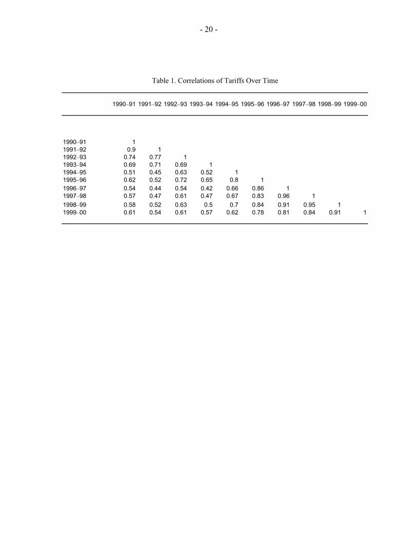
Figure 1A shows the average tariff for the 72 manufacturing industries in the 1980s and the 1990s. The average tariff in manufacturing increased from 86 percent in 1980–81 to 117 percent in 1990–91, and then declined to 39 percent in 1999–2000. In comparison, the trade reforms in Brazil reduced the average tariff level in manufacturing from about 60 percent in 1987 to 15 percent in 1998; in Colombia, from 50 percent to 13 percent between 1984 and 1998. Between 1980 and 1990, the average tariffs in Mexico decreased from 23 percent to 13 percent. Thus, the percentage point reduction in average tariffs between 1990–91 and 1999–2000 was much more drastic in India than in the trade liberalization episodes in the Latin American countries (Figure 1B). The level of protection varied widely across industries. The standard deviation of the tariff rate was 0.23 in 1980–81. Imports in two most protected sectors, textiles and cotton spinning, faced tariffs of 118 percent and 115 percent respectively. There was a considerable drop in the dispersion of tariff rates in the post-reform period. In 1999–2000, the standard deviation of the tariff rates dropped to 0.05. The trade reform also changed the structure of protection across industries. Figure 2 plots the tariffs in 1980–81 and 1999–2000 in various manufacturing industries. The tariffs declined in all the industries, and the decline differed across industries. Table 1 shows the year-to-year correlations for the tariffs since 1990–91. The pair-wise correlations range from 0.42 to 0.96. The intertemporal correlation of Indian tariffs is significantly lower than the correlation in U.S. tariffs. The correlation between U.S. tariffs in 1972 and 1988 is about 0.98. The low year-year correlation in the case of India is comparable to that in Brazil and Colombia (Blom et al., 2004, Goldberg and Pavcnik, 2004). In addition to tariffs, India also reduced nontariff barriers (NTBs) since 1991. The measure of nontariff barriers we have is the “import coverage ratio” which is defined as the share of imports subject to nontariff barriers. Figure 3 shows the average import coverage ratio in manufacturing in the 1980s and 1990s. The average import coverage ratio declined from 82 percent in 1990–91 to 17 percent in 1999–2000.

B. National Sample Survey Data The household survey data is drawn from the Employment-Unemployment Schedule of the National Sample Survey Organization (NSSO) administered by the Government of India. We use data from four survey rounds conducted in 1983–84 (38th round), 1987–88 (43rd round), 1993–94 (50th round), 1999–2000 (55th round). The data are a repeated cross-section. The data provide information on weekly earnings, worker characteristics e.g., age, education, gender, marital status, occupation, industry of employment at three-digit National Industrial Classification (NIC-1987) and state of residence. We restrict attention to workers in the urban areas who work in the manufacturing sector. We include workers between the ages of 15 and 65, who are a part of the labor force and report positive weekly earnings.

- 10 -

The measure of wages is weekly earnings in rupees, which are deflated by the consumer price index from the International Financial Statistics. Based on completed years of schooling, workers are divided into three categories―(i) primary or less: at most 5 years of schooling (ii) middle or secondary: 6–11 years of schooling (iii) higher secondary or more: at least 12 years of schooling.

VI. RESULTS

A. Estimation of Interindustry Wage Premiums

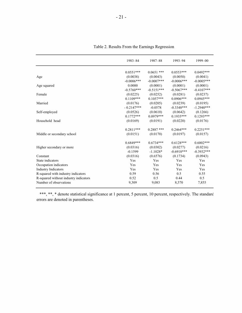
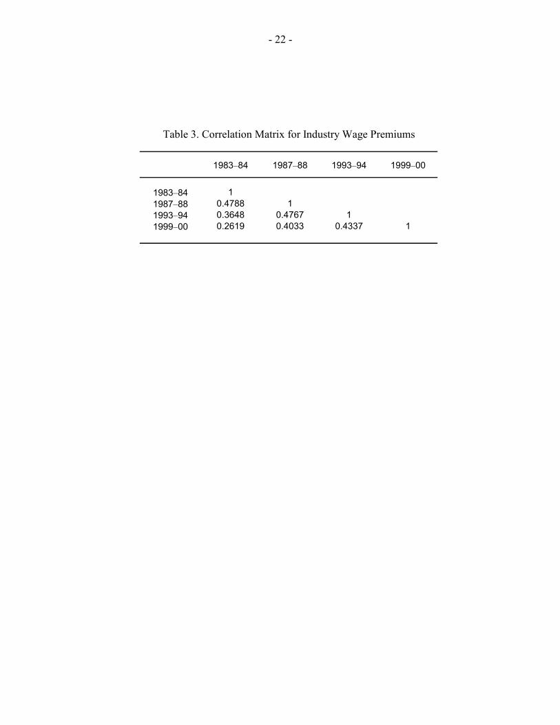
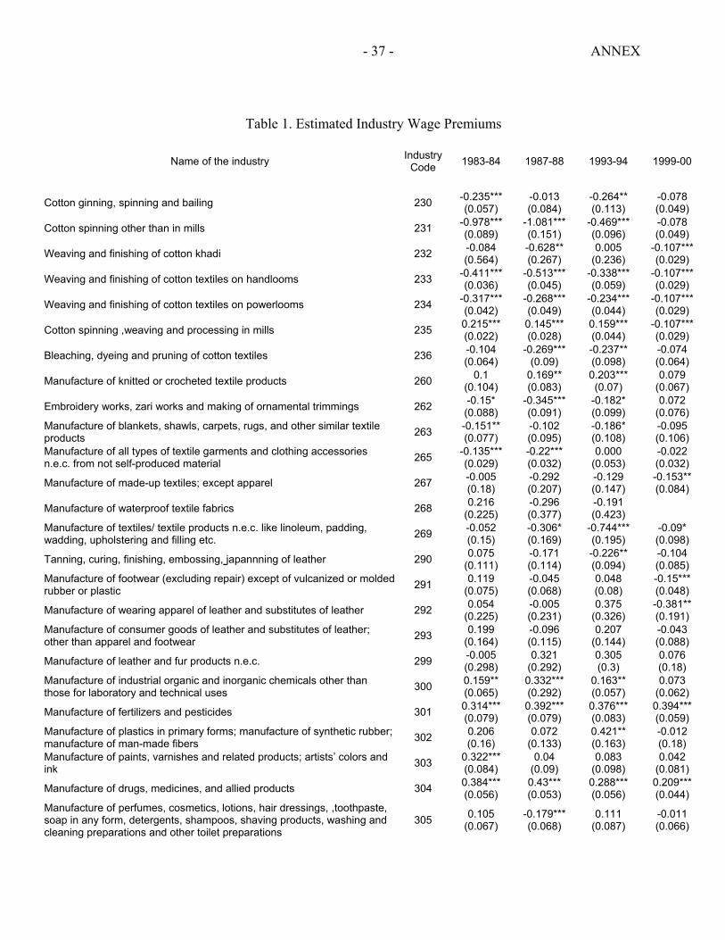
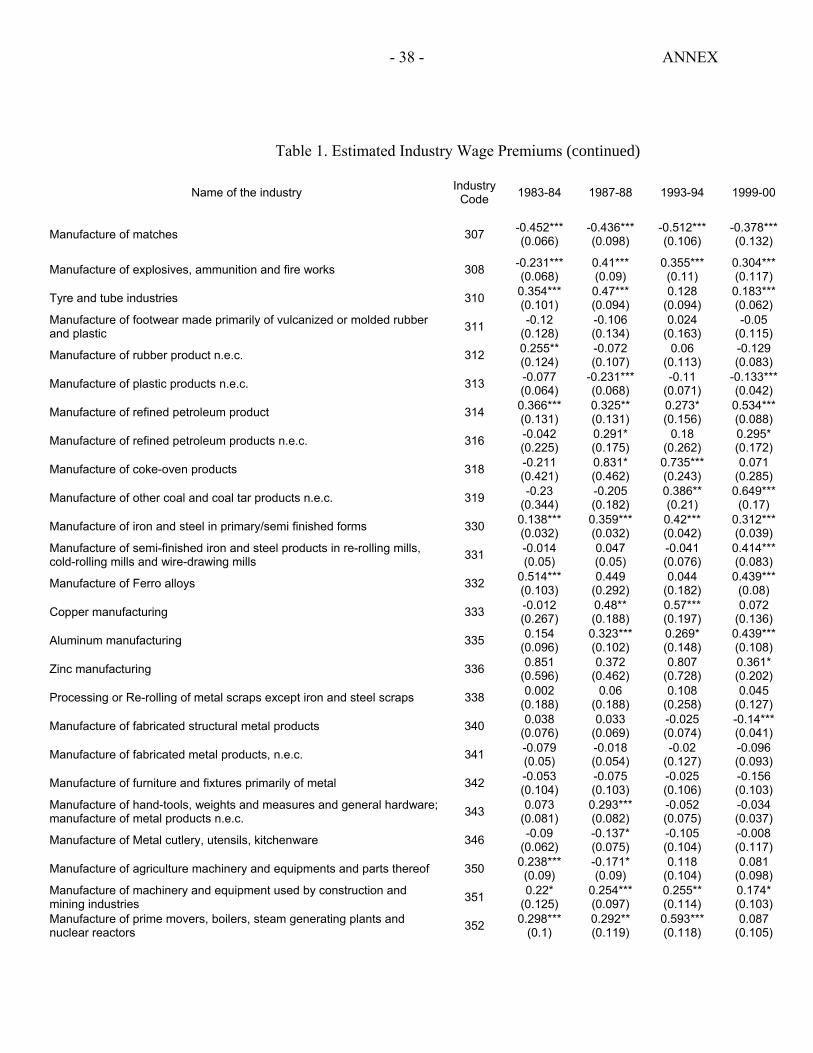
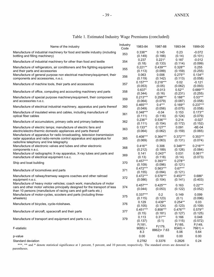
In the first stage, equation (1) is estimated separately for each round of the NSS. The logarithm of the individual worker’s wages are regressed on the dummies for worker’s industry affiliation, controlling for worker characteristics like age, age squared, dummies for education, marital status, gender, occupation, whether the individual is the head of the household and the state of residence. The first stage regression results are shown in Table 2. The bottom part of the table shows the R-squared for the regressions with and without industry dummies. For example, in 1999–2000, the R-squared for the regression excluding industry dummies is 0.50 i.e., the worker characteristics and state indicators alone explain about 50 percent of the variation in log weekly earnings. Adding the industry indicators increases the R-squared to 0.55 i.e., the industry indicators account for 5 percent of the total variation in log weekly earnings. In general, the industry indicators explain about 4 to 7 percent of the variation in log weekly earnings. Annex Table 1 shows the inter-industry wage premiums for the 72 three digit industries for which we have tariff data. The wage premiums are expressed as deviations from the employment weighted average wage premium. The standard errors are calculated by Haisken-DeNew and Schmidt (1997) procedure. The wage premiums are jointly statistically significant at 1 percent level (p-value = 0.00) in all the years. Many of the wage premiums are individually statistically significant as well. There is moreover, considerable dispersion in the wage premiums across industries. The standard deviations range from 0.24 to 0.34 for the different years. In 1983–84, the three highest wage premium industries are zinc manufacturing, office, computing and accounting machinery, and ferro alloys, and the lowest wage industries are cotton spinning, matches, and weaving and finishing of cotton textiles on handlooms. For example, the estimate of wage premium in manufacture of fertilizer and pesticides (industry code = 301) is 0.314, and the estimate of wage premium in weaving and finishing of cotton khadi (industry code = 232) is –0.084. These estimates imply that a worker with the same observable characteristics switching from leather footwear to khadi would observe a decline of 40 percent in weekly earnings (0.314-(-0.084)). The structure of wage premiums across industries has also changed over time. To examine the change in structure of the wage premiums, we look at their year-year correlations in Table 3. The correlation between the wage premiums in 1983–84 and 1999–2000 is 0.26, and

- 11 -

the correlation between the premiums in 1987–88 and 1999–2000 is 0.40. The Indian wage premiums are much less correlated over time than the wage premiums in the United States and Brazil (Krueger and Summers (1998), Goldberg and Pavcnik (2004)). The correlation coefficients are of the order of 0.9 for the United States (between 1974 and 1984) and Brazil (between 1987 and 1998). The low correlation between the wage premiums suggests that the structure of interindustry wage premiums changed significantly over time. Given that there were major trade reforms during the sample period, changes in trade policy could potentially constitute an explanation for the changing structure of the wage premiums.

B. Why Do Industry Wage Premiums Exist in India?

There is hardly any evidence on why industry wage differentials exist in developing countries. We do some simple exercises to test some of the explanations in the case of India. One possible explanation for the existence of wage premiums in a developing country like India could be the lack of perfect mobility of labor across sectors. There is evidence of significant labor market rigidities in India (e.g., see Dutt, 2003; Fallon and Lucas, 1993). India is ranked forty-fifth for the degree of labor market flexibility in the Global Competitiveness Report (GCR, 1998). Employment security in India is regulated mainly on the basis of the Industrial Disputes Act of 1947 (IDA). According to the 1982 amendment of the IDA, any firm employing 100 or more workers requires permission from the government before laying off or retrenching its workers. To test for evidence of labor reallocation between sectors, we also regress employment share of each industry, on tariff rates, industry and year indicators. The coefficient is 0.001 and is statistically insignificant. Thus, we do not find evidence for any significant employment sensitivity to trade shocks. This is consistent with the existence of labor market rigidities in developing countries like India. Various studies from other developing countries like Mexico and Colombia have found similar results (Revenga, 1997; Hanson and Harrison, 1999; Attanasio et al., 2004). The explanation for the existence of industry wage premiums based on imperfect mobility across sectors is ruled out in the case of the United States, since studies have shown that there is remarkable stability in the pattern of industry wage premiums over time (Dickens and Katz, 1987). However, this is not the case for India and as we argued in Section VI.1, the structure of industry wage premiums changed over time in India. This provides additional support for the view that industry wage premiums could exist due to labor market rigidities. A preliminary test of the labor quality explanation is to explore the impact of alternative degrees of control for human capital on inter-industry variation. If industry wage differentials were due to measured and unmeasured labor quality differences across industries, we would expect a substantial fall in the dispersion of industry wages once we control for measured human capital (Krueger and Summers, 1988). In our data, the addition of human capital controls―education, age, age squared (which is a proxy for tenure)―the drop in the standard

- 12 -

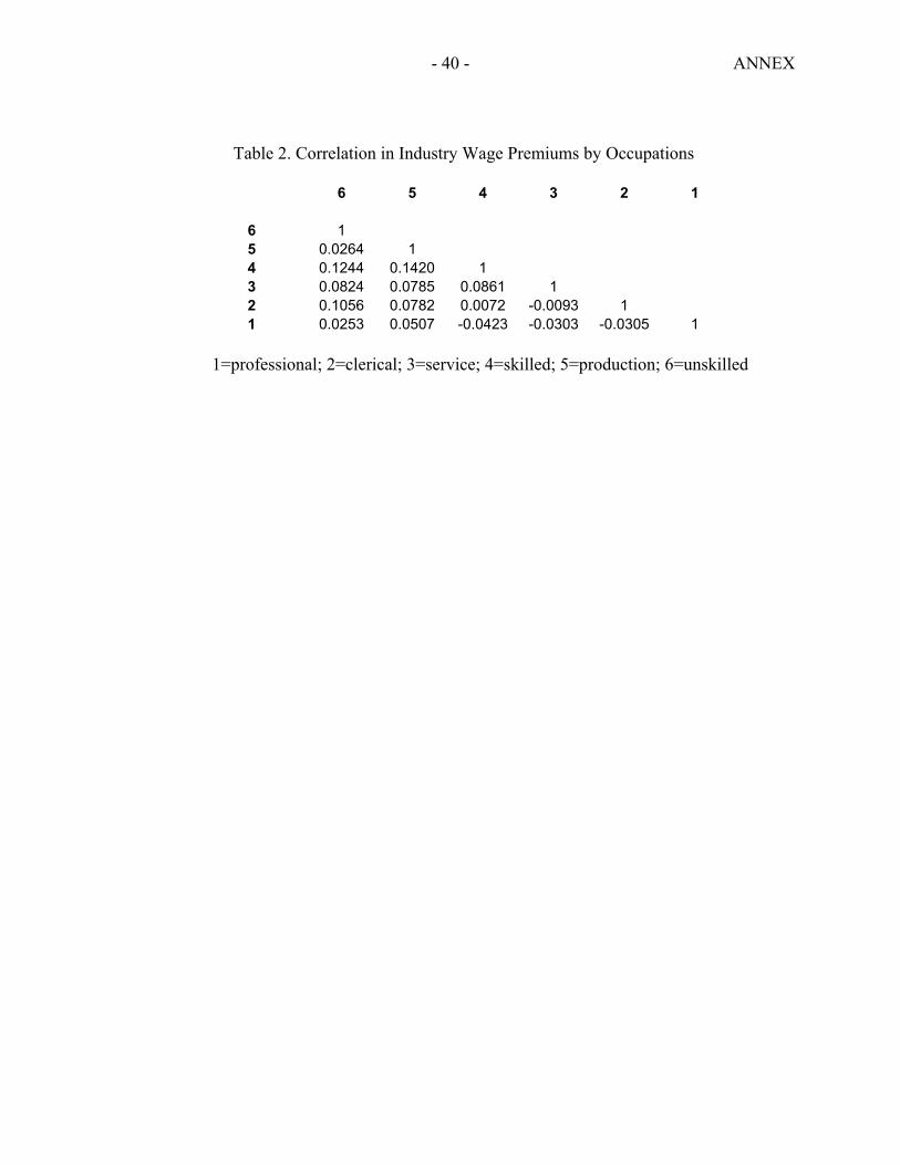
deviation of industry wage differentials ranges from 5 to 6 percentage points. Despite the increased controls for labor quality, the standard deviation is substantial and ranges from 24–34 percent. Unless one believes that variation in unmeasured labor quality is vastly more important than variation in age, tenure, and schooling, this evidence makes it difficult to attribute inter-industry wage differences to differences in labor quality. However, more conclusive evidence on labor quality explanation would require longitudinal data on wages of the same worker as he switches industries, where we can control for unobserved worker characteristics. One thing that many explanations for industry wage differentials have in common is that while they would lead us to expect differences in wages across industries for individual occupation groups, they would not lead us to expect the pattern of differentials to be similar for diverse occupations. In the United States, the high correlations of wage differentials in different occupations across industries cast doubt on explanations based on labor quality differences, compensating differentials and efficiency wages. For example, there is little reason to expect that an industry with dangerous production jobs which pays its blue-collar workers more to compensate them for the risks their jobs entail, would also pay its secretaries more. Technology might explain why one type of worker in a given industry would have some special unobservable skill, but it is much more difficult to explain why all occupations in such industries must be highly paid. Working conditions, skill requirements, and monitoring problems are also quite likely to differ across occupations in a firm or industry (Dickens and Katz, 1987). In the Indian case, we examine the correlation of industry wage differentials of different occupations across industries. Annex Table 2 shows the correlation of six occupation groups across industries. The correlations are much lower than that for the United States (see Dickens and Katz, 1987, Table 3). Unlike the United States, we do not find evidence in India that if one occupational group in an industry is highly paid relative to its observable characteristics, all categories of workers will tend to be high paid. Thus we cannot reject explanations based on labor quality differences, compensating differentials or efficiency wages based on the correlation in wage premiums of different occupational groups. Another potential explanation for industry wage differentials could be varying degrees of union bargaining power across industries. If the industry wage differences are due to “strong” unions that can raise wages without suffering severe employment losses in certain industries, we would expect to find less variability in wages across industries for nonunion workers (Krueger and Summers, 1988). However, this is not the case for India. In India, in 1993–94, non-union workers have slightly higher wage dispersion (=0.389) than union workers (=0.340).3 3 Unfortunately, all the National Sample Survey rounds do not record the union/non-union status of the workers.

- 13 -

Krueger and Summers (1988) also find similar results for the United States. The substantial wage dispersion across industries that exists even for the sample of non-union workers suggests that industry wage differences may not be a union phenomenon. However, the correlation between the wage premiums for the union and non-union workers in India (=0.225) is lower than that in the United States, (0.6–0.8, Dickens and Katz, 1987; Krueger and Summers, 1988). Additionally, there is also evidence that unions are not very powerful in India (Dutt, 2003). The Trade Union Act of 1926 provides for the registration and operation of trade unions. This act allows any seven workers to register their trade unions. This has led to multiplicity of unions with outsiders playing a prominent role. There is no procedure to determine the representative union, which would serve as a single bargaining unit. The outsiders controlling the unions are not really concerned about the genuine interests of the workers and pursue their own agenda. Also, the Industrial Disputes Act of 1947 confers upon the state the power to regulate labor-management relations. The inclusion of the state in the dispute settlement mechanisms complicates the bargaining process since the state itself is the dominant employer in the organized sector. To sum up, no single model fits all the facts. We would need much richer data to test for efficiency wage and labor quality explanations. The existence of unions does not seem to explain the existence of large wage differentials across industries. Labor market rigidities seem to be a plausible explanation for the existence of wage premiums.

C. Industry Wage Premiums and Trade Policy

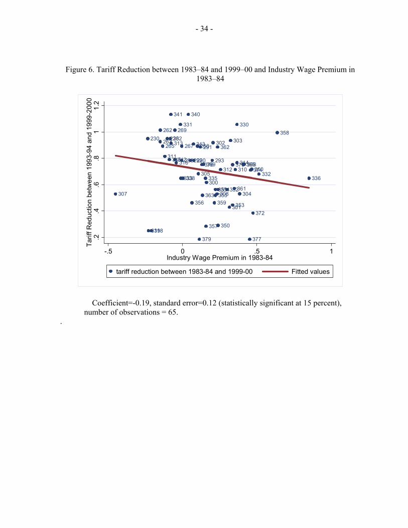
Preliminary Evidence First we look at some simple scatter plots to examine the characteristics of industries which had the greatest reduction in tariffs. Figure 4 shows the scatter plot for tariff reductions between 1983–84 and 1999–2000 and the tariffs in 1980. The raw data shows a strong and positive relationship between the tariff reduction between the two decades and the initial tariffs (coefficient=0.66, standard error=0.09) i.e., the magnitude of tariff reductions were greater in those industries with the highest initial tariff in 1980. Figure 5 shows the scatter plot for tariff reductions between 1983–84 and 1999–2000, and the share of unskilled workers in 1983. Unskilled workers are defined as those having less than 12 years of completed schooling. The raw data show a strong and positive relationship between tariff reduction and share of unskilled workers i.e. the greatest tariff reductions were in sectors with the highest share of unskilled workers. The tariff reductions were also the greatest in the low wage industries. Figure 6 shows the relationship between the magnitude of the tariff reductions and the wage premiums in 1983−84. There is a strong and negative correlation between the two (coefficient=-0.19, s.e.=0.12). Figures 4–6 are consistent with the evidence from Colombia, Brazil, and Mexico.

- 14 -

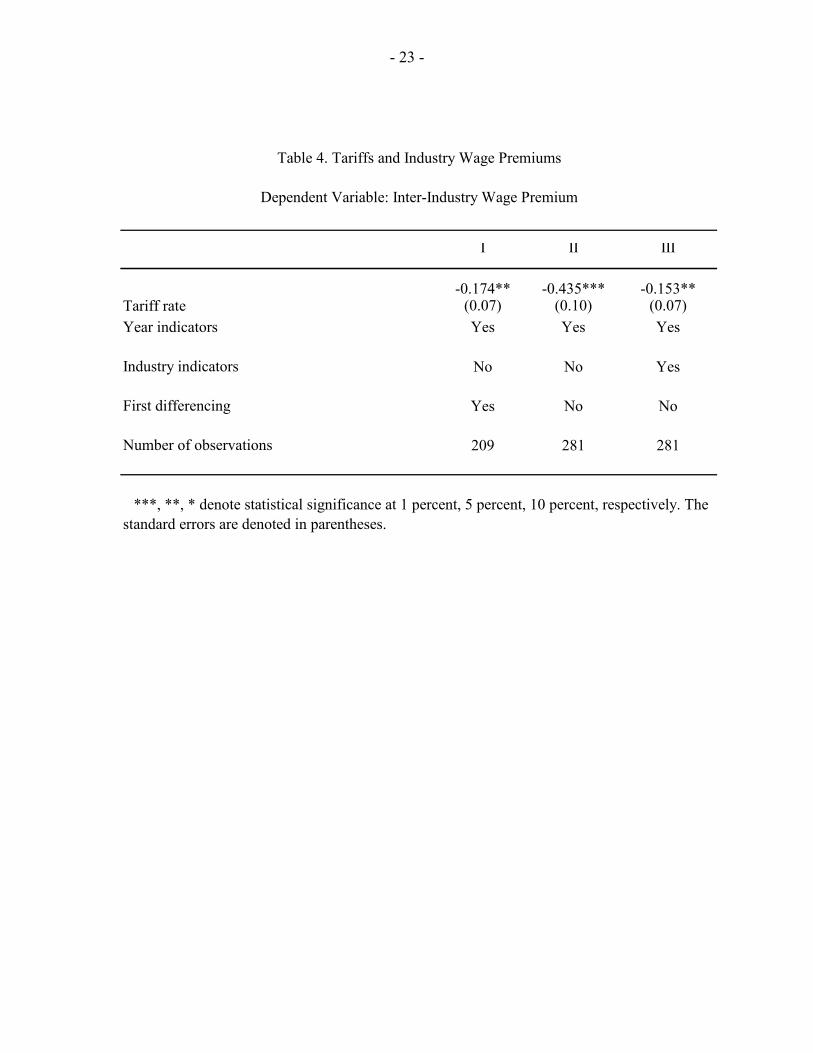
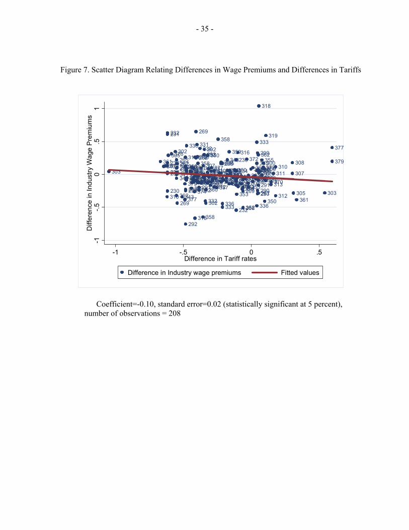
The existing studies on Colombia, Brazil and Mexico have also found that the tariff reductions were the greatest in industries with high pre-liberalization tariffs, low wage premiums, and high share of unskilled workers (Goldberg and Pavcnik, 2004; Blom et al., 2004; Hanson and Harrison, 1999).4 Before analyzing the relationship between wage premiums and trade policy in a regression framework, we look at the scatter diagram (Figure 7) relating changes in tariffs and changes in industry wage premiums (1983–84 to 1988–89, 1988–89 to 1993–94, 1993–94 to 1999−2000). Each point in the scatter plot represents the change in tariffs and the change in wage premiums within an industry between two consecutive time periods. The plot illustrates a strong and negative relationship between changes in tariffs and wage premiums. The raw data show that the growth in wage premium is highest for those industries that had the greatest tariff reductions. Second Stage Regressions: Wage Premiums and Tariffs In the second stage regression, the estimated industry wage premiums are regressed on tariffs, along with additional controls. The sample consists of all industries with available tariff information (72 industries). The results are shown in Table 4. Specification I shows the results for the first differenced specification corresponding to (2). The first differenced specification accounts for unobserved time-invariant industry specific factors. Specification II shows the results in levels without the industry indicators. Specification III shows the results in levels with industry indicators. Year indicators are included in all the specifications. The estimate of the coefficient of tariffs is negative and statistically significant (at 5 percent in specifications I and III, and at 1 percent in specification II). The negative coefficient on tariffs implies that increasing protection in a particular industry lowers wages in that industry. A coefficient of -0.17 in Specification 1 indicates that if the tariffs are reduced from 50 percent to 0 percent in a sector, average wage in that sector increases by 8.5 percent (0.17x0.5). Controlling for Nontariff Barriers: As shown in Figure 3, nontariff barriers (NTBs) were an important part of the trade liberalization process in India as well. We augment the basic regression to include our measure of NTBs―“import coverage ratio.” However, nontariff barriers are plagued with 4 In India, sectors with high share of unskilled workers which receive more protection also had lower import penetration ratio. Grossman and Helpman (1994) political economy model of protection predicts a negative correlation between import penetration ratio and protection for organized sectors. (See Goldberg and Pavcnik, 2003, for a similar explanation for Colombia).

- 15 -

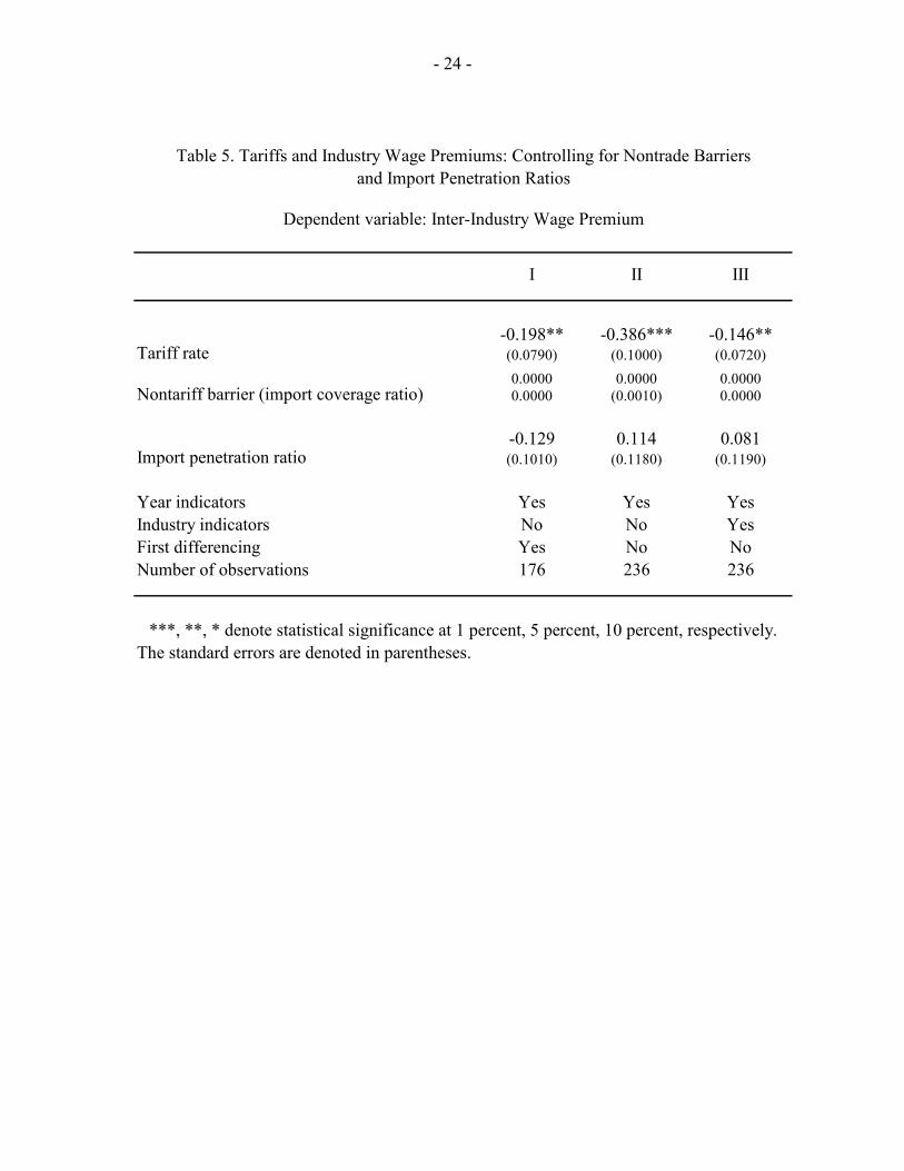
measurement errors and there is not much variation over time. Hence we focus on tariffs as our principal measure of trade policy and check the robustness of the coefficient on tariffs by including NTBs. We also augment the basic regression with import penetration ratios (defined as imports/output+imports-exports). Some of the effects of NTBs may be captured indirectly through the import measures. The results are shown in Table 5. These regressions include only those industries for which we have data on tariffs, import coverage ratio and import penetration ratio. The coefficient on tariffs remain negative and statistically significant (at least at 5 percent level) in all the specifications. The coefficient on the import coverage ratio is statistically insignificant in all the specifications.

D. Discussion of the Results

Dutt (2003) is the only other paper, which looks at the impact of trade liberalization on wages in India. Unlike this paper which uses detailed micro level data allowing us to control for worker characteristics, Dutt (2003) uses highly aggregated data on wages by industry. He finds a negative and statistically significant relationship between growth rate of wages and tariffs within a sector. Reduction in tariffs is associated with an increase in wage growth within a three-digit industry. However, he does not find a statistically significant relationship between changes in wage levels and changes in tariffs. The negative relationship between tariffs and wage premiums in this paper is similar to the results for the U.S. Gaston and Trefler (1994) find a negative relationship between protection and wage premiums in the U.S. manufacturing industries in 1983. They also control for the simultaneity bias in the cross-sectional data by instrumenting for trade protection. The coefficient on tariffs becomes more negative in the instrumental variable regressions. However, unlike Gaston and Trefler who examine the relationship between trade and industry wage premiums using cross sectional data, we exploit both the variation across industries and over time which allows us to control for industry specific heterogeneity. The results in this paper are in contrast to earlier work on Colombia, Mexico and Brazil. In case of Colombia, Goldberg and Pavcnik (2004) find a positive and statistically significant relationship between tariffs and wage premiums. In the case of Mexico, there is mixed evidence using data on workers earnings from two different sources. Revenga (1997) finds a positive relationship between industry wages and tariffs whereas Feliciano (2001) finds a negative but statistically insignificant relationship between industry wage premiums and tariffs. In their study of Brazil, Blom et al (2004) find a negative but statistically insignificant relationship between tariffs and wage premiums. Goldberg and Pavcnik (2004) find that the coefficient on tariffs is negative when industry indicators are not included in the estimation. When industry indicators are included, or when the regression is estimated in first differences, they find that the sign of the coefficient is reversed from negative to positive. The reversal of the sign of the coefficient when the model

- 16 -

is estimated in first differences is interpreted as the importance of time invariant political economy determinants of tariffs. Similar to Pavcnik and Goldberg (2004), we also find that the coefficient is negative when we estimate the regression without differencing (i.e., without controlling for time invariant industry specific heterogeneity (see Table 4, Column II). However, unlike them, we find that the coefficient remains negative even after first differencing (Table 4, Column I), but the magnitude of the coefficient does in fact decrease. Why has the impact of trade reform on worker wages in India been different from Colombia, Brazil and Mexico? Unlike Mexico and Colombia, in Brazil, the structure of industry wages did not change over time. Blom et al (2004) suggest that this could be one possible explanation for the insignificant relationship between tariffs and industry wages in Brazil. Given that the structure of industry wage premiums has changed over time in India as well, the significant relationship between trade policy and industry wage premiums is not surprising. However, what is striking is the negative sign of the coefficient on tariffs unlike the other developing countries. The negative relationship between trade liberalization and industry wage differentials in the Indian case is consistent with liberalization induced productivity changes at the firm level. There is evidence that the 1991 trade reforms led to higher levels and growth of firm productivity in India (Krishna and Mitra (1998), Aghion et al. (2003), Topalova (2004)). To the extent that productivity enhancements are passed onto industry wages, reductions in trade barriers would be associated with increase in wages within an industry. The relationship between trade policy and industry wage premiums has important implications for the impact of trade liberalization on wage inequality. Since different industries employ different shares of skilled workers, changes in industry wage premiums translate into changes in relative incomes of skilled and unskilled workers. Since the tariff reductions were relatively larger in sectors with a higher proportion of unskilled workers (Figure 5) and these sectors experienced an increase in relative wages, these unskilled workers experienced an increase in incomes relative to skilled workers. Thus, the findings in this paper suggest that trade liberalization has led to decreased wage inequality in India.

E. Endogeneity Issues

The industry fixed effects control for time-invariant unobserved industry specific heterogeneity. However, if there are unobserved time-varying industry specific factors that affect wages, they are not controlled for in the empirical specification. If the time varying, industry-specific factors are uncorrelated with the tariff rates, then the coefficient of interest would be unbiased. However, if they are correlated with the tariff rates, then the estimates would be biased. Some examples could be political economy factors that simultaneously affect tariff formation and industry wages, tariff changes in other industries etc.

- 17 -

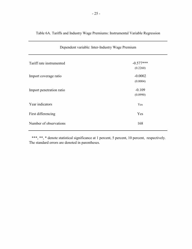
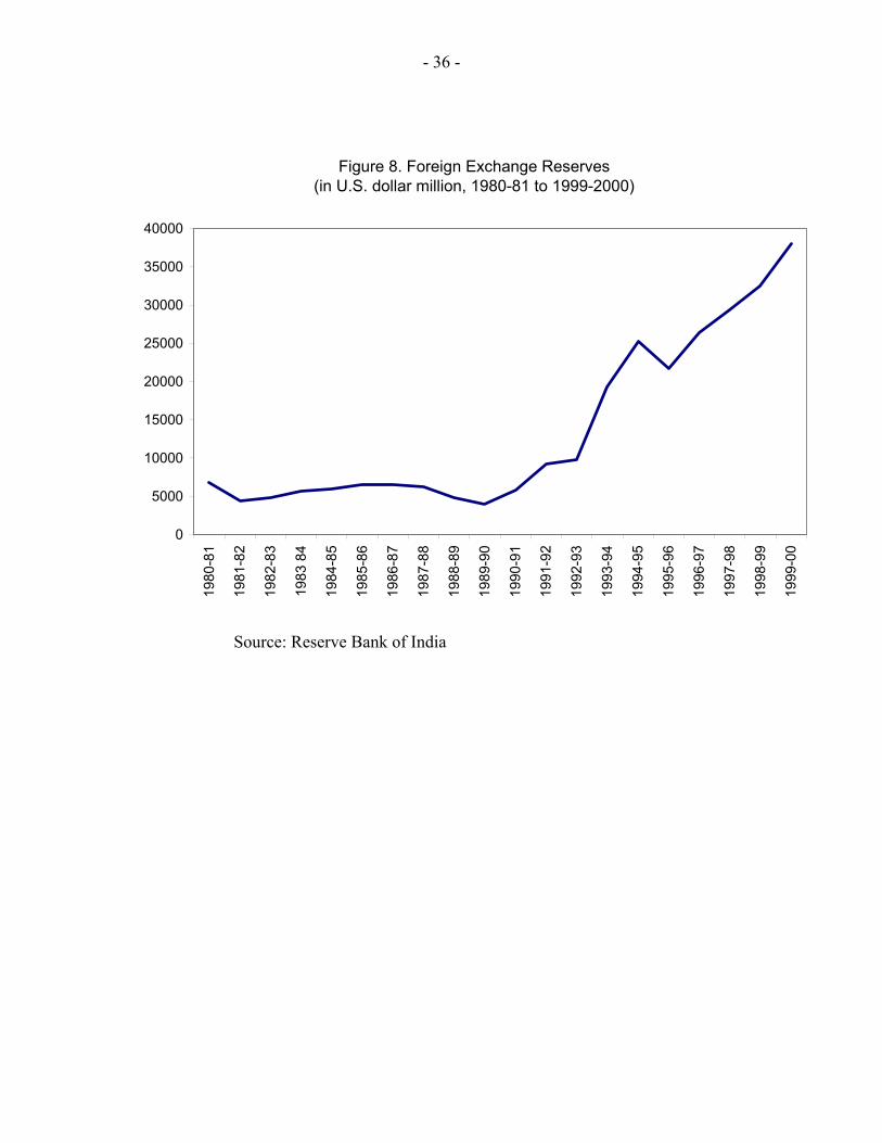
To address the above concern, we apply an instrumental variables strategy. An ideal instrument should be highly correlated with tariffs and uncorrelated with the industry specific time-varying unobserved component of wages.5 To construct industry-specific time varying instruments, we look at what constitutes variation in tariffs across sectors, and over time. The post-1991 trade reforms in India were in response to a severe balance of payments crisis. By mid-1991, the foreign exchange reserves were only enough to sustain two-weeks of imports. India took external assistance from the IMF, and the following trade reforms were a part of the structural conditionalities agreed by India. Hence, the variation in foreign exchange reserves can be expected to be correlated with tariff changes over time. Figure 8 shows the evolution of foreign exchange reserves in India over time. To explain the variation in tariff changes across sectors, following Goldberg and Pavcnik (2004), we use pre-reform tariffs in 1980 (1980 is the earliest period for which we have the tariff data), and the share of unskilled workers by industry (in 1983) as a determinant of tariff changes. We construct two industry-specific time varying instruments for tariff reductions: (i) interactions of foreign exchange reserves with tariff rates in 1980 (ii) interactions of foreign exchange reserves with share of unskilled workers in 1983. Table 6 shows the results from the instrumental variable regressions. The first stage regression results are shown in Table 6b. In the first stage we relate the changes in tariffs (1983 to 1987–88, 1987–88 to 1993–94, 1993–94 to 1999–2000) to the instruments. Nontrade barriers and import coverage ratio are also included in the regressions. The first stage results indicate a strong and statistically significant relationship between the change in tariffs and the two instruments. The R-squared of the first stage regression is 0.65. The two identifying instruments are also jointly statistically significant in the first stage regression (F-statistic = 13.1, p-value =0). Table 6A shows the second stage regression results. The coefficient of tariff rate is negative and statistically significant at 1 percent. The magnitude of the estimate is bigger than the comparable non-IV estimate in Table 4 (Column I). Gaston and Trefler (1994) also find that the tariff coefficient becomes more negative when they instrument for trade protection using industry characteristics. We also do a test of over identifying restrictions to check the validity of the instruments. We fail to reject the over-identifying restrictions at 1 percent and 5 percent levels, thus supporting the validity of the instruments.6 5 Since tariff rate is our principal measure of trade policy, we focus on instrumenting for the tariffs, assuming that NTBs are exogenous.

6 The chi-squared test statistic is 0.1056 when we exclude difference in reserves interacted with share of unskilled workers in the IV regression, and is 0.2992 when we exclude

(continued)

- 18 -

F. Additional Robustness Checks

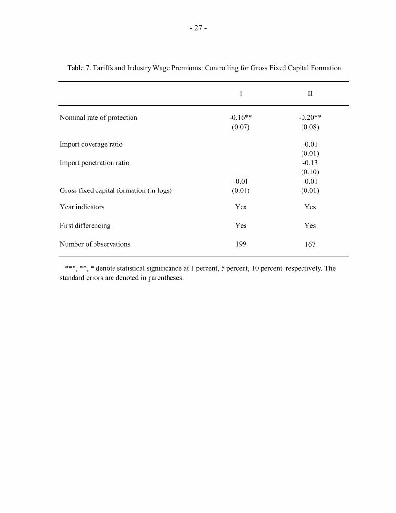
One time varying and industry specific variable which can be expected to affect wage premiums and also be correlated with tariff changes is sector-specific capital. To check the robustness of the results, we include gross fixed capital formation by sector as an additional regressor. Goldberg and Pavcnik (2004) also use gross fixed capital formation as a measure of capital accumulation in their study on Colombia. The data on gross fixed capital formation is taken from the Annual Survey of Industries (2002). The results are shown in Table 7. Gross fixed capital formation is included in levels for 1983–84, 1987–88 and 1993–94. The coefficient on tariffs is very similar to those in Tables 4 and 5 (Column 1). The coefficient on our measure of nontariff barriers is also very similar to that in Table 5 (Column 1). Thus, the negative correlation between tariffs and wage premiums is not driven by our measure of capital accumulation.

VII. CONCLUSIONS

This paper investigates the effects of trade policy on wages in Indian manufacturing industries in the last two decades. The data set combines micro labor market data from the National Sample Survey with data on tariff and nontariff barriers. Our results suggest that there is a significant relationship between trade policy and industry wage premiums. We find that increasing protection in a sector lowers wages in that sector. In sectors with largest tariff reductions, wages increased relative to the economy-wide average. The results are consistent with liberalization induced productivity increases at the firm level, which get passed onto industry wages. The findings in this paper are in contrast to studies on other developing countries like Colombia, Brazil, and Mexico, which have found either a positive or an insignificant relationship between trade policy and industry wage premiums. Our result is similar to the Gaston and Trefler (1994) study for the United States, who find a negative relationship between tariffs and industry wage premium. However, unlike Gaston and Trefler who use a cross-sectional data, our results are identified by using variation in wages and tariffs across industries as well as over time. Since the tariff reductions were relatively larger in sectors with a higher proportion of unskilled workers and these sectors experienced an increase in relative wages, these unskilled

difference in reserves interacted with tariffs in 1980 in the IV regression. The critical values of chi-squared with one degree of freedom is 6.64 and 3.84 at 1 percent and 5 percent levels respectively.

- 19 -

workers experienced an increase in incomes relative to skilled workers. Thus, the findings in this paper suggest that trade liberalization has led to decreased wage inequality in India.

- 20 -

Table 1. Correlations of Tariffs Over Time

1990–91 1991–92 1992–93 1993–94 1994–95 1995–96 1996–97 1997–98 1998–99 1999–00

1990–91 11991–92 0.9 11992–93 0.74 0.77 11993–94 0.69 0.71 0.69 11994–95 0.51 0.45 0.63 0.52 11995–96 0.62 0.52 0.72 0.65 0.8 11996–97 0.54 0.44 0.54 0.42 0.66 0.86 11997–98 0.57 0.47 0.61 0.47 0.67 0.83 0.96 11998–99 0.58 0.52 0.63 0.5 0.7 0.84 0.91 0.95 11999–00 0.61 0.54 0.61 0.57 0.62 0.78 0.81 0.84 0.91 1

- 21 -

Table 2. Results From the Earnings Regression

1983–84 1987–88 1993–94 1999–00

0.0551*** 0.0651 *** 0.0553*** 0.0492***(0.0038) (0.0043) (0.0050) (0.0041)

-0.0006*** -0.0007*** -0.0006*** -0.0005***0.0000 (0.0001) (0.0001) (0.0001)

-0.5760*** -0.5151*** -0.5067*** -0.4107***(0.0225) (0.0252) (0.0281) (0.0237)

0.1109*** 0.1057*** 0.0906*** 0.0945***(0.0176) (0.0205) (0.0239) (0.0195)

- 0.2147*** -0.0578 -0.3348*** -1.2940***(0.0526) (0.0610) (0.0642) (0.1266)

0.1772*** 0.0979*** 0.1935*** 0.1293***(0.0169) (0.0191) (0.0220) (0.0176)

0.2811*** 0.2887 *** 0.2464*** 0.2251***(0.0151) (0.0170) (0.0197) (0.0157)

0.6849*** 0.6734*** 0.6128*** 0.6002***(0.0316) (0.0302) (0.0277) (0.0216)-0.1599 -1.1028* -0.6918*** -0.3932***(0.0316) (0.6576) (0.1734) (0.0943)

State indicators Yes Yes Yes YesOccupation indicators Yes Yes Yes YesIndustry Indicators Yes Yes Yes YesR-squared with industry indicators 0.59 0.56 0.5 0.55R-squared without industry indicators 0.52 0.5 0.44 0.5Number of observations 9,309 9,083 8,570 7,855

***, **, * denote statistical significance at 1 percent, 5 percent, 10 percent, respectively. The standarderrors are denoted in parentheses.

Constant

Self-employed

Household head

Middle or secondary school

Higher secondary or more

Age

Age squared

Female

Married

- 22 -

Table 3. Correlation Matrix for Industry Wage Premiums

1983–84 1987–88 1993–94 1999–00

1983–84 11987–88 0.4788 11993–94 0.3648 0.4767 11999–00 0.2619 0.4033 0.4337 1

- 23 -

Table 4. Tariffs and Industry Wage Premiums

Dependent Variable: Inter-Industry Wage Premium

I II III

-0.174** -0.435*** -0.153**(0.07) (0.10) (0.07)

Year indicators Yes Yes Yes

Industry indicators

First differencing

Number of observations

***, **, * denote statistical significance at 1 percent, 5 percent, 10 percent, respectively. Thestandard errors are denoted in parentheses.

Tariff rate

No No Yes

Yes No No

209 281 281

- 24 -

Table 5. Tariffs and Industry Wage Premiums: Controlling for Nontrade Barriersand Import Penetration Ratios

Dependent variable: Inter-Industry Wage Premium

I II III

-0.198** -0.386*** -0.146**(0.0790) (0.1000) (0.0720)0.0000 0.0000 0.0000 0.0000 (0.0010) 0.0000

-0.129 0.114 0.081(0.1010) (0.1180) (0.1190)

Year indicators Yes Yes YesIndustry indicators No No YesFirst differencing Yes No NoNumber of observations 176 236 236

***, **, * denote statistical significance at 1 percent, 5 percent, 10 percent, respectively.The standard errors are denoted in parentheses.

Tariff rate

Nontariff barrier (import coverage ratio)

Import penetration ratio

- 25 -

Table 6A. Tariffs and Industry Wage Premiums: Instrumental Variable Regression

Dependent variable: Inter-Industry Wage Premium

-0.577***(0.2260)

-0.0002(0.0004)

-0.109(0.0990)

Year indicators Yes

First differencing Yes

Number of observations 168

***, **, * denote statistical significance at 1 percent, 5 percent, 10 percent, respectively.The standard errors are denoted in parentheses.

Tariff rate instrumented

Import coverage ratio

Import penetration ratio

- 26 -

Table 6B. First Stage Instrumental Variable Regression

Dependent Variable: Tariff Rate

Tariff rate in 1980 interacted with foreign exchange reserves -0.295***(0.0790)

Share of unskilled workers in 1983 interacted with foreign exchange reserves -0.312*(0.1840)

0.001*(0.0003)

0.0820 (0.0860)

Year Indicators Yes

First differencing Yes

Number of observations 168

R-squared 0.65

***, **, * denote statistical significance at 1 percent, 5 percent, 10 percent, respectively. Thestandard errors are denoted in parentheses.

Import coverage ratio

Import penetration ratio

- 27 -

Table 7. Tariffs and Industry Wage Premiums: Controlling for Gross Fixed Capital Formation

I II

Nominal rate of protection -0.16** -0.20**(0.07) (0.08)

Import coverage ratio -0.01(0.01)

Import penetration ratio -0.13(0.10)

-0.01 -0.01Gross fixed capital formation (in logs) (0.01) (0.01)

Year indicators Yes Yes

First differencing Yes Yes

Number of observations 199 167

***, **, * denote statistical significance at 1 percent, 5 percent, 10 percent, respectively. Thestandard errors are denoted in parentheses.

- 28 -

Figure 1A. Average Tariff Rates in Manufacturing (1980-81 to 1999-2000)

0

20

40

60

80

100

120

14019

80-8

1

1981

-82

1982

-83

1983

-84

1984

-85

1985

-86

1986

-87

1987

-88

1988

-89

1989

-90

1990

-91

1991

-92

1992

-93

1993

-94

1994

-95

1995

-96

1996

-97

1997

-98

1998

-99

1999

-00

In p

erce

nt

The average tariff rates are for 72 three-digit manufacturing industries classified according to the National Industrial Classification 1987 (NIC-1987).

- 29 -

Figure 1B. Average Tariff Rates: India and Latin America(1980-81 to 1999-2000)

0

20

40

60

80

100

120

140

1980

1981

1982

1983

1984

1985

1986

1987

1988

1989

1990

1991

1992

1993

1994

1995

1996

1997

1998

1999

2000

In p

erce

nt

India (Manu)Colombia(Manu)Brazil(Manu)Mexico (All industries)

- 30 -

Figure 2. Tariffs: Pre and Post Liberalization

- 31 -

Figure 3. Non-Tariff Barriers: Average Import Coverage Ratio (1980-81 to 1999-2000)

0.0

0.1

0.2

0.3

0.4

0.5

0.6

0.7

0.8

0.9

1.0

1980

-81

1981

-82

1982

-83

1983

-84

1984

-85

1985

-86

1986

-87

1987

-88

1988

-89

1989

-90

1990

-91

1991

-92

1992

-93

1993

-94

1994

-95

1995

-96

1996

-97

1997

-98

1998

-99

1999

-00

Import coverage ratio is defined as the share of imports subject to nontariff barriers. The average import coverage ratios are for 72 three-digit manufacturing industries classified according to the National Industrial Classification 1987 (NIC-1987).

- 32 -

Figure 4. Tariff Reduction and Pre-Liberalization Tariffs

Coefficient = 0.66 (se=0.09), statistically significant at 1 percent, number of observations = 72.

- 33 -

Figure 5. Tariff Reduction and Share of Unskilled Workers

230232 236260

262

263265267

269

290

291

292 293 299

300

301

302 303

304

305

307308

310

311

312

313

314 316

318 319

330 331

332333 335 336338

340341

342

343

346

350

351352

353

354355

356

357

358

359

360

361

362

363

365368 369

372

374375 376

377379.2.4

.6.8

11.

2Ta

riff R

educ

tion

betw

een

1993

-94

and

1999

-200

0

.5 .6 .7 .8 .9 1Share of Unskilled Workers in 1983-84

tariff reduction between 1983-84 and 1999-00 Fitted values

Coefficient=0.71, standard error=0.25, statistically significant at 1 percent level, number of observations = 65. Unskilled workers are defined as those having less than 12 years of completed schooling.

- 34 -

Figure 6. Tariff Reduction between 1983–84 and 1999–00 and Industry Wage Premium in 1983–84

230 232236260

262

263265 267

269

290

291

292 293299

300

301

302 303

304

305

307 308

310

311

312

313

314316

318319

330331

332333 335 336338

340341

342

343

346

350

351 352

353

354355

356

357

358

359

360

361

362

363

365368369

372

374375376

377379.2.4

.6.8

11.

2Ta

riff R

educ

tion

betw

een

1993

-94

and

1999

-200

0

-.5 0 .5 1Industry Wage Premium in 1983-84

tariff reduction between 1983-84 and 1999-00 Fitted values

Coefficient=-0.19, standard error=0.12 (statistically significant at 15 percent), number of observations = 65.

.

- 35 -

Figure 7. Scatter Diagram Relating Differences in Wage Premiums and Differences in Tariffs

230

231

232

233

234235236

260

262

263

265

267

268

269 290291292

293

299

300301

302

303

304

305

307

308310

311

312

313314

316

318

319330331

332

333

335

336

338340341

342

343

346

350

351352

353

354

355

356357

358

359

360

361

362

363365368

369

370

371372

374375

376377

379

230

231232

233

234235236260262

263

265267268

269

290

291

292293

299

300

301

302

303

304

305

307308

310

311312313

314316 318

319

330

331

332

333

335

336

338340341 342

343

346

350

351

352

353354

355

356

357

358

359360

361

362

363365368

369370

371

372

374

375376

377

379

230

232

236

260

262

263265267

269

290

291

292

293299

300301

302

303304305

307

308310

311312

313

314

316

318

319

330

331332

333

335

336

338340341342

343346

350351

352

353354

355356 357

358

359

360361

362

363365368

369

372

374375

376

377

379

-1-.5

0.5

1D

iffer

ence

in In

dust

ry W

age

Pre

miu

ms

-1 -.5 0 .5Difference in Tariff rates

Difference in Industry wage premiums Fitted values

Coefficient=-0.10, standard error=0.02 (statistically significant at 5 percent), number of observations = 208

- 36 -

Figure 8. Foreign Exchange Reserves (in U.S. dollar million, 1980-81 to 1999-2000)

0

5000

10000

15000

20000

25000

30000

35000

4000019

80-8

1

1981

-82

1982

-83

1983

84

1984

-85

1985

-86

1986

-87

1987

-88

1988

-89

1989

-90

1990

-91

1991

-92

1992

-93

1993

-94

1994

-95

1995

-96

1996

-97

1997

-98

1998

-99

1999

-00

Source: Reserve Bank of India

- 37 - ANNEX

Table 1. Estimated Industry Wage Premiums

Name of the industry Industry Code 1983-84 1987-88 1993-94 1999-00

Cotton ginning, spinning and bailing 230 -0.235*** (0.057)

-0.013 (0.084)

-0.264** (0.113)

-0.078 (0.049)

Cotton spinning other than in mills 231 -0.978*** (0.089)

-1.081*** (0.151)

-0.469*** (0.096)

-0.078 (0.049)

Weaving and finishing of cotton khadi 232 -0.084 (0.564)

-0.628** (0.267)

0.005 (0.236)

-0.107*** (0.029)

Weaving and finishing of cotton textiles on handlooms 233 -0.411*** (0.036)

-0.513*** (0.045)

-0.338*** (0.059)

-0.107*** (0.029)

Weaving and finishing of cotton textiles on powerlooms 234 -0.317*** (0.042)

-0.268*** (0.049)

-0.234*** (0.044)

-0.107*** (0.029)

Cotton spinning ,weaving and processing in mills 235 0.215*** (0.022)

0.145*** (0.028)

0.159*** (0.044)

-0.107*** (0.029)

Bleaching, dyeing and pruning of cotton textiles 236 -0.104 (0.064)

-0.269*** (0.09)

-0.237** (0.098)

-0.074 (0.064)

Manufacture of knitted or crocheted textile products 260 0.1 (0.104)

0.169** (0.083)

0.203*** (0.07)

0.079 (0.067)

Embroidery works, zari works and making of ornamental trimmings 262 -0.15* (0.088)

-0.345*** (0.091)

-0.182* (0.099)

0.072 (0.076)

Manufacture of blankets, shawls, carpets, rugs, and other similar textile products 263 -0.151**

(0.077) -0.102 (0.095)

-0.186* (0.108)

-0.095 (0.106)

Manufacture of all types of textile garments and clothing accessories n.e.c. from not self-produced material 265 -0.135***

(0.029) -0.22*** (0.032)

0.000 (0.053)

-0.022 (0.032)

Manufacture of made-up textiles; except apparel 267 -0.005 (0.18)

-0.292 (0.207)

-0.129 (0.147)

-0.153** (0.084)

Manufacture of waterproof textile fabrics 268 0.216 (0.225)

-0.296 (0.377)

-0.191 (0.423)

Manufacture of textiles/ textile products n.e.c. like linoleum, padding, wadding, upholstering and filling etc. 269 -0.052

(0.15) -0.306* (0.169)

-0.744*** (0.195)

-0.09* (0.098)

Tanning, curing, finishing, embossing, japannning of leather 290 0.075 (0.111)

-0.171 (0.114)

-0.226** (0.094)

-0.104 (0.085)

Manufacture of footwear (excluding repair) except of vulcanized or molded rubber or plastic 291 0.119

(0.075) -0.045 (0.068)

0.048 (0.08)

-0.15*** (0.048)

Manufacture of wearing apparel of leather and substitutes of leather 292 0.054 (0.225)

-0.005 (0.231)

0.375 (0.326)

-0.381** (0.191)

Manufacture of consumer goods of leather and substitutes of leather; other than apparel and footwear 293 0.199

(0.164) -0.096 (0.115)

0.207 (0.144)

-0.043 (0.088)

Manufacture of leather and fur products n.e.c. 299 -0.005 (0.298)

0.321 (0.292)

0.305 (0.3)

0.076 (0.18)

Manufacture of industrial organic and inorganic chemicals other than those for laboratory and technical uses 300 0.159**

(0.065) 0.332*** (0.292)

0.163** (0.057)

0.073 (0.062)

Manufacture of fertilizers and pesticides 301 0.314*** (0.079)

0.392*** (0.079)

0.376*** (0.083)

0.394*** (0.059)

Manufacture of plastics in primary forms; manufacture of synthetic rubber; manufacture of man-made fibers 302 0.206

(0.16) 0.072

(0.133) 0.421** (0.163)

-0.012 (0.18)

Manufacture of paints, varnishes and related products; artists’ colors and ink 303 0.322***

(0.084) 0.04

(0.09) 0.083

(0.098) 0.042

(0.081)

Manufacture of drugs, medicines, and allied products 304 0.384*** (0.056)

0.43*** (0.053)

0.288*** (0.056)

0.209*** (0.044)

Manufacture of perfumes, cosmetics, lotions, hair dressings, ,toothpaste, soap in any form, detergents, shampoos, shaving products, washing and cleaning preparations and other toilet preparations

305 0.105 (0.067)

-0.179*** (0.068)

0.111 (0.087)

-0.011 (0.066)

- 38 - ANNEX

Table 1. Estimated Industry Wage Premiums (continued)

Name of the industry Industry Code 1983-84 1987-88 1993-94 1999-00

Manufacture of matches 307 -0.452*** (0.066)

-0.436*** (0.098)

-0.512*** (0.106)

-0.378*** (0.132)

Manufacture of explosives, ammunition and fire works 308 -0.231*** (0.068)

0.41*** (0.09)

0.355*** (0.11)

0.304*** (0.117)

Tyre and tube industries 310 0.354*** (0.101)

0.47*** (0.094)

0.128 (0.094)

0.183*** (0.062)

Manufacture of footwear made primarily of vulcanized or molded rubber and plastic 311 -0.12

(0.128) -0.106 (0.134)

0.024 (0.163)

-0.05 (0.115)

Manufacture of rubber product n.e.c. 312 0.255** (0.124)

-0.072 (0.107)

0.06 (0.113)

-0.129 (0.083)

Manufacture of plastic products n.e.c. 313 -0.077 (0.064)

-0.231*** (0.068)

-0.11 (0.071)

-0.133*** (0.042)

Manufacture of refined petroleum product 314 0.366*** (0.131)

0.325** (0.131)

0.273* (0.156)

0.534*** (0.088)

Manufacture of refined petroleum products n.e.c. 316 -0.042 (0.225)

0.291* (0.175)

0.18 (0.262)

0.295* (0.172)

Manufacture of coke-oven products 318 -0.211 (0.421)

0.831* (0.462)

0.735*** (0.243)

0.071 (0.285)

Manufacture of other coal and coal tar products n.e.c. 319 -0.23 (0.344)

-0.205 (0.182)

0.386** (0.21)

0.649*** (0.17)

Manufacture of iron and steel in primary/semi finished forms 330 0.138*** (0.032)

0.359*** (0.032)

0.42*** (0.042)

0.312*** (0.039)

Manufacture of semi-finished iron and steel products in re-rolling mills, cold-rolling mills and wire-drawing mills 331 -0.014

(0.05) 0.047 (0.05)

-0.041 (0.076)

0.414*** (0.083)

Manufacture of Ferro alloys 332 0.514*** (0.103)

0.449 (0.292)

0.044 (0.182)

0.439*** (0.08)

Copper manufacturing 333 -0.012 (0.267)

0.48** (0.188)

0.57*** (0.197)

0.072 (0.136)

Aluminum manufacturing 335 0.154 (0.096)

0.323*** (0.102)

0.269* (0.148)

0.439*** (0.108)

Zinc manufacturing 336 0.851 (0.596)

0.372 (0.462)

0.807 (0.728)

0.361* (0.202)

Processing or Re-rolling of metal scraps except iron and steel scraps 338 0.002 (0.188)

0.06 (0.188)

0.108 (0.258)

0.045 (0.127)

Manufacture of fabricated structural metal products 340 0.038 (0.076)

0.033 (0.069)

-0.025 (0.074)

-0.14*** (0.041)

Manufacture of fabricated metal products, n.e.c. 341 -0.079 (0.05)

-0.018 (0.054)

-0.02 (0.127)

-0.096 (0.093)

Manufacture of furniture and fixtures primarily of metal 342 -0.053 (0.104)

-0.075 (0.103)

-0.025 (0.106)

-0.156 (0.103)

Manufacture of hand-tools, weights and measures and general hardware; manufacture of metal products n.e.c. 343 0.073

(0.081) 0.293*** (0.082)

-0.052 (0.075)

-0.034 (0.037)

Manufacture of Metal cutlery, utensils, kitchenware 346 -0.09 (0.062)

-0.137* (0.075)

-0.105 (0.104)

-0.008 (0.117)

Manufacture of agriculture machinery and equipments and parts thereof 350 0.238*** (0.09)

-0.171* (0.09)

0.118 (0.104)

0.081 (0.098)

Manufacture of machinery and equipment used by construction and mining industries 351 0.22*

(0.125) 0.254*** (0.097)

0.255** (0.114)

0.174* (0.103)

Manufacture of prime movers, boilers, steam generating plants and nuclear reactors 352 0.298***

(0.1) 0.292** (0.119)

0.593*** (0.118)

0.087 (0.105)

- 39 - ANNEX

Table 1. Estimated Industry Wage Premiums (concluded)

Name of the industry Industry Code 1983-84 1987-88 1993-94 1999-00

Manufacture of industrial machinery for food and textile industry (including bottling and filling machinery) 353 0.336**

(0.149) 0.145

(0.188) 0.23

(0.14) -0.072 (0.101)

Manufacture of industrial machinery for other than food and textile 354 0.237 (0.18)

0.221* (0.133)

0.187 (0.114)

-0.012 (0.099)

Manufacture of refrigerators, air conditioners and fire fighting equipment and their parts and accessories 355 0.221**

(0.113) 0.439*** (0.099)

0.328** (0.159)

0.255 (0.255)

Manufacture of general purpose non electrical machinery/equipment, their components and accessories, n.e.c. 356 0.063

(0.119) 0.006

(0.142) 0.275** (0.113)

0.134** (0.058)

Manufacture of machine tools, their parts and accessories 357 0.157*** (0.053)

0.218*** (0.05)

0.02 (0.062)

-0.121 (0.093)

Manufacture of office, computing and accounting machinery and parts 358 0.637* (0.344)

-0.013 (0.16)

0.52** (0.231)

0.689*** (0.255)

Manufacture of special purpose machinery/equipment, their component and accessories n.e.c. 359 0.213***

(0.064) 0.298*** (0.079)

0.188** (0.087)

0.53*** (0.058)

Manufacture of electrical industrial machinery, apparatus and parts thereof 360 0.465*** (0.049)

0.4*** (0.056)

0.169** (0.075)

0.237*** (0.058)

Manufacture of insulated wires and cables, including manufacture of optical fiber cables 361 0.348***

(0.111) -0.04

(0.116) 0.153

(0.124) 0.173** (0.079)

Manufacture of accumulators, primary cells and primary batteries 362 0.236** (0.111)

0.536*** (0.154)

0.214 (0.172)

-0.027 (0.152)

Manufacture of electric lamps; manufacture of electric fans and electric/electro-thermic domestic appliances and parts thereof 363 0.133**

(0.064) 0.127** (0.062)

0.091 (0.159)

-6E-04 (0.065)

Manufacture of apparatus for radio broadcasting, television transmission radar apparatus and radio-remote control apparatus and apparatus for radio/line telephony and line telegraphy

365 0.408*** (0.069)

0.364*** (0.063)

0.372*** (0.131)

0.353*** (0.074)

Manufacture of electronic valves and tubes and other electronic components n.e.c. 368 0.416**

(0.212) 0.306

(0.189) 0.348*** (0.126)

0.216*** (0.084)

Manufacture of radiographic X-ray apparatus, X-ray tubes and parts and manufacture of electrical equipment n.e.c. 369 0.141

(0.13) 0.243** (0.118)

0.031 (0.14)

0.061** (0.073)

Ship and boat building 370 0.457*** (0.109)

0.393*** (0.096)

0.278** (0.121)

Manufacture of locomotives and parts 371 0.472*** (0.155)

0.563*** (0.094)

0.67*** (0.121)

Manufacture of railway/tramway wagons coaches and other railroad equipment n.e.c. 372 0.472***

(0.086) 0.578*** (0.104)

0.453*** (0.141)

0.686* (0.403)

Manufacture of heavy motor vehicles; coach work; manufacture of motor cars and other motor vehicles principally designed for the transport of less than 10 persons (manufacture of racing cars and golf-carts etc.)

374 0.457*** (0.044)

0.425*** (0.053)

0.163 (0.122)

0.22*** (0.052)

Manufacture of motor-cycles, scooters and parts (including three-wheelers) 375 0.337***

(0.115) 0.2

(0.123) 0.149 (0.1)

0.099 (0.096)

Manufacture of bicycles, cycle-rickshaws. 376 0.129 (0.105)

0.439** (0.124)

0.254** (0.123)

0.03 (0.109)

Manufacture of aircraft, spacecraft and their parts 377 0.451*** (0.15)

0.858*** (0.181)

0.476*** (0.127)

0.579** (0.125)

Manufacture of transport and equipment and parts n.e.c. 379 0.113 (0.137)

0.31*** (0.1)

0.166 (0.115)

0.048 (0.572)

F-statistic F(181, 9085) =

8.3

F(179, 8862)= 7.63

F(185, 8340) =

5.06

F(149, 7661) =

5.64 p-value 0.00 0.00 0.00 0.00 Standard deviation 0.2782 0.3376 0.2826 0.24

***, ** and * denote statistical significance at 1 percent, 5 percent, and 10 percent, respectively. The standard errors are denoted in parentheses.

- 40 - ANNEX

Table 2. Correlation in Industry Wage Premiums by Occupations

6 5 4 3 2 1 6 1 5 0.0264 1 4 0.1244 0.1420 1 3 0.0824 0.0785 0.0861 1 2 0.1056 0.0782 0.0072 -0.0093 1 1 0.0253 0.0507 -0.0423 -0.0303 -0.0305 1

1=professional; 2=clerical; 3=service; 4=skilled; 5=production; 6=unskilled

- 41 -

REFERENCES Aghion, P., R. Burgess, S. Redding, and F. Zilibotti, 2003, “The Unequal Effects of

Liberalization: Theory and Evidence from India,” (unpublished; London School of Economics, London).

Annual Survey of Industries, 2002, “Database on the Industrial Sector in India: 1973–74 to

1997–98”, Mumbai: Economic and Political Weekly Research Foundation. Attanasio, O., P. Goldberg, and N. Pavcnik, 2004, “Trade Reforms and Wage Inequality in

Colombia,” Journal of Development Economics, Vol. 74, No. 4, pp. 331–66. Blom, A., P. Goldberg, N. Pavcnik, and N. Schady, 2004, “Trade Liberalization and Industry

Wage Structure: Evidence from Brazil,” World Bank Economic Review, forthcoming. Das, D.K., 2003, “Quantifying Trade Barriers: Has Protection Declined Substantially in

Indian Manufacturing? ICRIER,” Indian Council for Research on International Economic Relations Working Paper No. 105, New Delhi.

Dickens, W.T., and L.F. Katz, 1987, “Inter-Industry Wage Differentials and Theories of

Wage Discrimination,” NBER Working Paper No. 2271 (Cambridge, Massachusetts: National Bureau of Economic Research).

Dutt, P. 2003, “Labor Market Outcomes and Trade Reforms: The Case of India,” in The

Impact of Trade on Labor: Issues, Perspectives and Experiences from Developing Asia, ed. by R. Hasan and D. Mitra (Haarlem: North-Holland/Elsevier Science B.V., pp. 1–45).

Fallon, P.R. and R.E. Lucas, 1993, “Job Security Regulation and the Dynamic Demand for

Industrial Labor in India and Zimbabwe”, Journal of Development Economics, Vol. 40, No. 2, pp. 241–275.

Feliciano, Z., 2001, “Workers and Trade Liberalization: The Impact of Trade Reforms in

Mexico on Wages and Employment,” Industrial and Labor Relations Review, Vol. 55 No. 1, pp. 95–115.

Frankel, J. and Romer, D., 1999. “Does Trade Cause Growth?” American Economic Review,

Vol. 89 (June), pp. 379–399. Gaston, N., and D. Trefler, 1994, “Protection, Trade and Wages: Evidence from U.S.

Manufacturing.” Industrial and Labor Relations Review, Vol. 47, No. 4, pp. 574−593. Goldberg, P. and N. Pavcnik, 2004, “Trade, Wages, and the Political Economy of Trade

Protection: Evidence from the Colombian Trade Reforms,” Journal of International Economics, forthcoming.

- 42 -

Grossman, G.M., 1984, “International Competition and the Unionized Sector,” Canadian Journal of Economics, Vo. 17, No. 3, pp. 541–556.

Grossman, G.M. and E. Helpman, 1994, “Protection for Sale,” American Economic Review,

Vol. 84, No. 4, pp. 833–850. Haisken-DeNew, J.P. and C.M. Schmidt, 1997, “Inter-Industry and Inter-Region Wage

Differentials: Mechanism and Interpretation,” Review of Economics and Statistics, Vol. 79, No. 3, pp. 516–21.

Hanson, G. and A. Harrison, 1999, “Who Gains from Trade Reform? Some Remaining

Puzzles,” Journal of Development Economics, Vol. 59 (June), pp. 125–54. Harrison, A., 1994, “Productivity, Imperfect Competition and Trade Reform: Theory and

Evidence,” Journal of International Economics, Vol. 36, Nos. 1−2, pp. 53–73. Katz, L.F., L.H. Summers, R.E. Hall, C.L. Schultze and R.H. Topel, 1989, “Industry Rents:

Evidence and Implications,” Brookings Papers on Economic Activity. Microeconomics, Vol. 1989, pp. 209–90. Brookings Institution.

Krishna, P. and D. Mitra, 1998, “Trade Liberalization, Market Discipline and Productivity

Growth: New Evidence from India,” Journal of Development Economics, Vol. 56, No. 2 , pp. 447–462.

Krueger, A.B. and L.H. Summers, 1988, “Efficiency Wages and the Inter-Industry Wage

Structure,” Econometrica, Vol. 56, pp. 259–293. McDonald, I.M. and R.M. Solow, 1981, “Wage Bargaining and Unemployment,” American

Economic Review, Vol. 71 (December), pp. 896–908. National Sample Survey Organization (NSSO), 1983–84, 1987–88, 1993–94, 1999−2000,

“Employment and Unemployment, Schedule 10.0”, Ministry of Statistics and Program Implementation, Government of India.

Pavcnik, N., 2000, “Trade Liberalization, Exit and Productivity Improvements. Evidence

From Chilean Plants,” Review of Economic Studies, Vol. 69, pp. 245–76. Revenga, A., 1997, ‘Employment and Wage Effects of Trade Liberalization: The Case of

Mexican Manufacturing,” Journal of Labor Economics, Vol. 15, pp. S20–43. Topalova, P., 2004, “Trade Liberalization and Firm Productivity: The Case of India,” IMF

Working Paper 04/28 (Washington: International Monetary Fund). World Economic Forum, 1998, Global Competitiveness Report (Geneva).