The Impact of Income on Democracy Revisited

The Impact of Income on DemocracyRevisited

Yi Chea, Yi Lub, Zhigang Taoa,�and Peng Wangca University of Hong Kong

b National University of Singaporec Hong Kong University of Science & Technology

May 2012

Abstract

This paper revisits the important issue of whether economic de-velopment promotes democracy by using the system-GMM method,which is superior to the di¤erence-GMMmethod when dependent vari-ables (democracy in this paper) are highly persistent over time. Withthe same data set as that of Acemoglu, Johnson, Robinson, and Yared(2008), we �nd that the system-GMM estimated coe¢ cient of incomeper capita is positive and highly statistically signi�cant, in sharp con-trast to the di¤erence-GMM results reported by Acemoglu, Johnson,Robinson, and Yared (2008). Furthermore, employing the U.S. andColombia as an example, we �nd that much of the di¤erence in democ-racy across countries can be explained by the corresponding di¤erencein income per capita.

Keywords: Income, Democracy, System-GMM, Di¤erence-GMMJEL Codes: P16, O10

�Corresponding author: Zhigang Tao, Faculty of Business and Economics, The Univer-sity of Hong Kong, Pokfulam Road, Hong Kong. Tel: 852-2857-8223; Fax: 852-2858-5614;Email: [email protected]. We would like to thank Gérard Roland (the Editor), and two anony-mous referees for their useful comments and suggestions. Financial support from Univer-sity of Hong Kong and Hong Kong Research Grants Council is greatly acknowledged.

1

1 Introduction

A proposition of major and perennial interest to both economists and polit-ical scientists is whether economic development promotes democracy. Manystudies have reported a positive association between income per capita andthe degree of democracy (see, for example, Lipset, 1959; Barro, 1997, 1999;Papaioannou and Siourounis, 2008). However, establishing the causal impactof economic development on democracy is challenging, because there could beunobserved factors in�uencing both economic development and democracy(i.e., the omitted variables issue), and there may also be reverse causalityrunning from democracy to economic development. In a seminal paper, Ace-moglu, Johnson, Robinson, and Yared (2008) (AJRY) use the �xed e¤ectsspeci�cation to account for time-invariant unobserved factors, and surpris-ingly �nd no positive and statistically signi�cant relationship between incomeper capita and democracy.As the degree of democracy in an economy is highly persistent over time,

AJRY (2008) include the lagged value of democracy in their regression analy-sis. However, in their �xed e¤ects speci�cation, the di¤erence of the laggeddemocracy is correlated with the di¤erence of the error term, causing bi-ased estimations of the impact of income per capita. To address this prob-lem, AJRY (2008) use the di¤erence-GMM estimation method developed byArellano and Bond (1991), in which the di¤erence of lagged democracy isinstrumented by all the further available lags of democracy. Recent advancesin econometrics, however, show that these available lags of democracy onlyexplain a very small portion of the di¤erence of the lagged democracy (i.e.,the weak instrument problem; see Staiger and Stock, 1997; Stock andWright,2000; Stock, Wright, and Yogo, 2002) when the dependent variable is highlypersistent over time. To resolve this weak instrument problem, Arellano andBover (1995) and Blundell and Bond (1998) develop a new method calledthe system-GMM in which the di¤erence-GMM equations are stacked by thelevel equations where the lagged dependent variable is instrumented by thedi¤erence of the lagged dependent variable. In a simulation study of theAR(1) model,1 Bond (2002) shows that the system-GMM estimation alwaysoutperforms the di¤erence-GMM estimation, especially when the dependentvariable is highly persistent over time.2 Speci�cally, as shown in Table 1

1The model speci�cation is yit = �yi;t�1+(�i+�it), where i represents the panel unit;t represents time; �i is the panel �xed e¤ect; and �it is the error term.

2Many recent empirical studies have shown that the system-GMM estimator performsbetter than the di¤erence-GMM estimator; see, for example, Blundell and Bond (2000),Bobba and Coviello (2007), Castello-Climent (2008), Roodman (2009a), and Aslaksen(2010).

2

(copied from Table 2 of Bond, 2002), the di¤erence-GMM estimate of � is0:484 (or 0:226) when the true value is 0:8 (or 0:9), whereas the correspondingsystem-GMM estimate is 0:810 (or 0:941).Democracy is indeed highly persistent over time. In Table 2, we present

various estimation results of the �rst-order auto-regression of democracy.The OLS estimated coe¢ cient is 0:866, which is usually considered the up-per bound, whereas the panel �xed e¤ect estimated coe¢ cient is 0:419, whichis often considered the lower bound. The most valid estimate is 0:817 ob-tained from the t�3 system-GMM estimation, as it satis�es the identi�cationassumptions implied by the insigni�cant Hansen J test and the insigni�cantdi¤erence Hansen J test. Because of the highly persistent nature of democ-racy (i.e., with the AR(1) coe¢ cient being 0:817), the coe¢ cient of the laggeddemocracy in the AJRY (2008) di¤erence-GMM estimation is only weaklyidenti�ed and biased, causing the estimated coe¢ cient of income per capitato be biased or even misleading. In this paper, we use the system GMMestimation method to revisit the impact of income per capita on democracywith the same data set as that employed by AJRY (2008) (downloaded fromthe AER web site).We �nd that under the system-GMM estimation, the estimated coe¢ cient

of income per capita becomes positive and highly statistically signi�cant, insharp contrast to the results AJRY (2008) obtain from the di¤erence-GMMmethod. We then conduct a series of robustness checks: �ve exercises mir-roring those of AJRY (2008) (an alternative measure of democracy, di¤erentsub-samples, additional controls, external instrumental variables for incomeper capita, and longer sample periods and longer time intervals for variablemeasurement), one exercise the same as that conducted by AJRY (2009) (dif-ferential impacts across countries with di¤erent initial degrees of democracy),one exercise similar to that of Boix (2011) (di¤erent sample periods), one ex-ercise including the additional controls used by Boix and Stokes (2003), Boix(2011), and Miller (forthcoming), and a new exercise (extending the analysisto more recent years). In all these exercises, we �nd that the coe¢ cient ofincome per capita is always positive and statistically signi�cant. As a furtherrobustness check, we follow AJRY (2008) in calculating the extent to whichour estimation results explain variations in the degree of democracy acrosscountries. Using Colombia as an example, we �nd that if we elevate incomeper capita in Colombia to the level of the United States in 2000, our esti-mation results explain almost all the di¤erence in democracy between thesetwo countries. Overall, this study lends strong support to the modernizationhypothesis that economic development promotes democracy (Lipset, 1959).Several other recent studies have challenged the robustness of the results

of AJRY (2008). Boix (2011) overturns the main results of AJRY (2008)

3

by extending the data to the early nineteenth century, when hardly anycountries were democratic, and by adopting a broader theory of developmentand international relations. Benhabib, Corvalan, and Spiegel (2011) alsore-establish the positive impact of development on democracy by utilizingnewer income data and using estimation methods to deal with the problemof measures of democracy being censored. Our paper di¤ers from these twostudies by using the same data sets as those employed by AJRY (2008),but we reverse the results of AJRY (2008) by adopting the system GMMestimation method, which is considered more suitable than the panel �xede¤ects estimation or di¤erence-GMM estimation method when the dependentvariable (i.e., democracy in this paper) is highly persistent over time.Our paper is also related to the literature regarding the exogenous theory

of democracy (i.e., that development has a positive impact on the stability ofa democratic country) versus the endogenous theory of democracy (i.e., thatdevelopment has a positive impact on the transition of an autocratic countryto a democratic one). Przeworski and Limongi (1997) and Przeworski, Al-varez, Cheibub, and Limongi (2000) �nd that development helps democraticcountries become less likely to revert to autocracy (i.e., providing supportfor the exogenous theory of democracy), but it has a limited e¤ect on thedemocratization of autocratic countries (i.e., no supporting the endogenoustheory of democracy). Boix and Stokes (2003), however, �nd evidence sup-porting both the exogenous and endogenous theories of democracy by bothextending the data to the early nineteenth century and including more controlvariables.3 Similar to Boix and Stokes (2003), we o¤er evidence supportingboth the endogenous and exogenous theories of democracy by adopting thesystem-GMM estimation method to examine the same data set as that usedby AJRY (2008, 2009), and the extended data set used by Boix and Stokes(2003) and Boix (2011).The rest of the paper is organized as follows. Section 2 discusses the

data set and model speci�cations employed for empirical analysis. Section 3presents our empirical �ndings. The paper concludes in Section 4.

3Miller (2011) further elaborates on why the endogenous theory of democracy may notwork. Speci�cally, as income per capita increases, the probability of a social uprising inan autocratic country is likely to decrease, but the chance of a transition to democracy incase of a social uprising would increase. Treisman (2011) shows that the positive impactof economic development on democracy is more pronounced in the medium run (10 to 20years), which explains why even dictators may still focus on development in the short run,as it helps them to entrench themselves in power.

4

2 Data and Model Speci�cation

The data set used in this paper is the same as that examined by AJRY(2008) (downloaded from the American Economic Review web site4). Themain measure of democracy is the Freedom House Political Rights Index5

augmented by Bollen�s data.6 As a robustness check, we use the CompositePolity Index7 from the Polity IV project as an alternative measure of democ-racy. Both the Freedom House measure of democracy and the Polity measureof democracy are normalized to [0; 1], with a higher value indicating a higherdegree of democracy. Information about income per capita comes from thePenn World Table for the post-war period and from the study of Maddison(2010) for the pre-war period beginning in 1820.Following AJRY (2008), we use a dynamic panel data model to investigate

the causal impact of income per capita on democracy:

dit = �dit�1 + yit�1 +X0

it�1� + �t + �i + "it; (1)

where dit is the degree of democracy for country i in period t; dit�1 is thelagged democracy variable used to account for the persistence of democracyover time; yit�1, the main variable of interest in this study, is the lagged logincome per capita; Xit�1 is a vector of control variables; �t denotes the unob-served time e¤ect controlling for common shocks originated from macroeco-nomic, political, or technological sources; �i is the �xed e¤ect which controlsfor the unobserved time-invariant country-speci�c characteristics; and "it isthe error term. To account for possible heteroskedasticity, standard errorsare clustered at the country level.To deal with the correlation between �i and dit�1 in (1), a �rst-di¤erence

transformation can be used to purge the country �xed e¤ect �i:

�dit = ��dit�1 + �yit�1 +�X0

it�1� +��t +�"it; (2)

where � is the �rst-di¤erence operator, e.g., �dit = dit � dit�1. BecauseCov(�dit�1;�"it) 6= 0 due to the fact that dit�1 is a function of "it�1, theOLS estimation of (2) produces a biased estimate of �; and as a consequence,the estimate of �the main parameter of interest �is also biased.

4Web site: http://www.aeaweb.org/issue.php?journal=AER&volume=98&issue=35The Freedom House Political Rights Index ranges from 1 to 7 with a lower value

indicating a higher degree of democracy. As the �rst year of the Freedom House PoliticalRights Index is 1972, AJRY (2008) use the value of democracy in 1972 for that of 1970 intheir �ve-year interval analysis.

6Bollen�s data allow us to extend the �ve-year interval analysis from 1970 to 1950.7The Composite Polity Index ranges from �10 to 10; with a higher value indicating a

higher degree of democracy.

5

For the consistent estimation of (2), Arellano and Bond (1991) use thedi¤erence-GMM method �rst proposed by Holtz-Eakin, Newey, and Rosen(1988) in which dit�2 and all the further available lags are used as instrumentsfor �dit�1 given there is no second-order serial correlation in �"it. Thevalidity of the proposed instruments can be justi�ed by assuming E ("it) =E ("itdit�j) = 0 for j = 1; 2; :::t � 1. This corresponds to the followingorthogonality condition for (2):

E[A0

i��i] = 0; (3)

where ��i = (�"i3;�"i4; :::;�"iT )0and

Ai =

2664di1 0 0 ::: 0 ::: 00 di1 di2 ::: 0 ::: 0: : : ::: : ::: :0 0 0 ::: di1 ::: diT�2

3775 :Arellano and Bond (1991) suggest using the AR(2) test to check whetherthere is any second-order serial correlation of �"it, and recommend using theHansen J test to check for possible violation of the orthogonality condition(3).However, as pointed out in the Introduction, the di¤erence-GMMmethod

su¤ers from a severe weak instrument problem when the dependent variableis highly persistent over time. This renders both point estimates and hypoth-esis tests unreliable (Staiger and Stock, 1997; Stock and Wright, 2000; Stock,Wright and Yogo, 2002). Arellano and Bover (1995) and Blundell and Bond(1998) argue that when the dependent variable is highly persistent over time,the di¤erence of the lagged dependent variable has more explanatory powerfor the lagged dependent variable than that of the available lags of the de-pendent variable for the di¤erence of the lagged dependent variable. Hence,they propose augmenting the di¤erence-GMM method with the original levelequation (1) in which the lagged �rst-di¤erenced dependent variable is usedas the instrument for the lagged dependent variable. This brings a set ofadditional orthogonality conditions as follows:

E[�dit�1(�i + "it)] = 0; (4)

the validity of which can be tested by the di¤erence Hansen J test as proposedby Arellano and Bover (1995) and Blundell and Bond (1998). This methodis referred to as the �system-GMM�. Given that the degree of democracyin a country is highly persistent over time, we plan to revisit the impact ofincome per capita on democracy using the system-GMM method.

6

It is worth noting that as the instrument count grows with the timedimension T , the Hansen J test for the orthogonality condition (3) or thedi¤erence Hansen J test for the orthogonality condition (4) might su¤er fromnotable size distortion as documented by Andersen and Sorensen (1996),Bowsher (2002), and Roodman (2009b). Roodman (2009b) also discussesother symptoms of instrument proliferation studied in the literature such asover�tting endogenous variables, imprecise estimates of the GMM optimalweighting matrix, and bias in two-step standard errors. Extensive simulationstudies conducted by Roodman (2009b) suggest that collapsing instruments,a way to reduce the instrument count, tends to mitigate �nite sample biasand greatly increase the ability of the Hansen J and di¤erence Hansen Jtests to detect violation of orthogonality conditions. When reporting ourempirical results, we follow this practice by adding the estimates obtainedfrom collapsing instruments.

3 Empirical Findings

3.1 Main Results

Columns 1-2 of Table 3 summarize our system-GMM estimation results re-garding the impact of income per capita on democracy (i.e., the FreedomHouse measure of democracy) for the 1960-2000 period,8 where both the de-pendent and independent variables are measured over a �ve-year interval.9

For ease of comparison, the results from the pooled OLS, panel �xed e¤ectand di¤erence-GMM estimations are copied from those of AJRY (2008) inColumns 3-5 of Table 3.As shown in Column 3, the pooled OLS estimation gives a positive and

statistically signi�cant estimated coe¢ cient of income per capita, consistentwith the �ndings of Barro (1997, 1999). However, as discovered by AJRY(2008), the coe¢ cient of income per capita becomes statistically insigni�cant,but positive, once the country �xed e¤ects are controlled for (Column 4),and it becomes signi�cantly negative under the di¤erence-GMM estimation(Column 5). Interestingly, we �nd that the estimated coe¢ cient of incomeper capita reverts to a positive and highly statistically signi�cant value underthe system-GMM estimation (Column 1).

8For the details of the data and the construction of variables, please see AJRY (2008).9We use the one-step GMM estimation adopted by AJRY (2008) to make our results

comparable with theirs, though the results from the two-step GMM estimation with smallsample correction (Windmeijer, 2005) are qualitatively the same (available upon request).We also follow AJRY (2008) in using a double lag to instrument income per capita in theGMM estimation.

7

Our system-GMM estimation is valid, as the insigni�cance of the AR(2)test result implies no second-order serial correlation of the error term, theinsigni�cance of the Hansen J test result suggests the satisfaction of orthog-onality condition (3), and the insigni�cance of the di¤erence Hansen J testresult implies the satisfaction of orthogonality condition (4). More impor-tantly, the estimated coe¢ cient of lagged democracy (0:574) is rather high,lying well between the lower limit of �xed e¤ects estimate (0:379) and theupper limit of pooled OLS estimate (0:706). The high persistence of thedegree of democracy in a country over time is expected to lend more cre-dence to the results of the system-GMM estimation than it is to those of thedi¤erence-GMM estimation (Bond, 2002).As a way of checking whether or not our system-GMM estimation re-

sults make sense, we conduct a counterfactual analysis investigating whethervariations in the degree of democracy across countries can be explained bytheir di¤erences in income per capita. We follow AJRY (2008) by comparingthe U.S. with Colombia as an illustration. The �rst two pillars in Figure1 are the democracy scores (measured by the Freedom House index) of theU.S. and Colombia in 2000, respectively. Given that our estimated coe¢ -cient of income per capita is 0:102 (Column 1 of Table 3), the short-runimpact of income per capita on democracy in Colombia would be an in-crease of (10:41� 8:59)� 0:102 = 0:187 if Colombia�s log income per capitawere lifted from 8:59 to the level of the U.S. (i.e., 10:41). The long-run im-pact of income per capita on democracy in Colombia would be an increase of0:187�(1�0:574) = 0:438, where 0:574 is the coe¢ cient of the lagged democ-racy (Column 1 of Table 3). These two degrees of democracy for Colombiaare presented in pillars 3 and 4 of Figure 1, respectively. It is interesting tonote that the height of pillar 4 is almost the same as that of pillar 1, indi-cating that the di¤erence in income per capita between Colombia and theUnited States explains most of the di¤erence in democracy between the twocountries.To check the robustness of our system-GMM estimates, we also report re-

sults from the system-GMM estimation with collapsing instruments, aimedat alleviating the instrument proliferation problem in the system-GMM es-timation. Using collapsing instruments barely changes either the magnitudeor statistical signi�cance of the system-GMM estimates (Column 2 of Table3). Meanwhile, the system-GMM estimates with collapsing instruments passthe various speci�cation tests: the Hansen J test, the di¤erence Hansen Jtest, and the AR(2) test.

8

3.2 Robustness checks

In the following section, we conduct a series of robustness checks: �ve exer-cises the same as those conducted by AJRY (2008) (an alternative measure ofdemocracy, di¤erent sub-samples, additional controls, external instrumentalvariables for income per capita, and longer sample periods and longer timeintervals for variable measurement), one exercise the same as that employedby AJRY (2009) (di¤erential impacts across countries with di¤erent initialdegrees of democracy), one exercise similar to that of Boix (2011) (di¤erentsample periods), one exercise including the additional controls used by Boixand Stokes (2003), Boix (2011) and Miller (forthcoming), and a new exercise(extending the analysis to more recent years).Alternative measure of democracy. In the main analysis above, we

use the Freedom House measure of democracy augmented by Bollen�s data,which cover only the post-1950 period. As a robustness check, we use an al-ternative measure of democracy, Polity IV, which provides information for allindependent countries starting in 1800. The system-GMM estimation resultsobtained using the Polity measure of democracy are reported in Column 1 ofTable 4. We �nd a positive and statistically signi�cant coe¢ cient of incomeper capita. This result is consistent with our earlier system-GMM results(Column 1 of Table 3) and contrast sharply with the results of the panel�xed e¤ects and di¤erence-GMM estimations reported by AJRY (2008).Di¤erent sub-samples. In Columns 2-3 of Table 4, we present our

system-GMM estimation results for two sub-samples to address two possiblesampling concerns in line with the approach of AJRY (2008). First, wefocus on a balanced sample of countries from 1970 to 2000 to make sure ourresults are not a¤ected by the entry and exit of countries during the sampleperiod. Second, we focus on a sub-sample excluding former socialist countriesto alleviate the concern that our results could be a¤ected by the inclusionof these countries, which experienced a surge in democracy yet underwentsigni�cant economic decline in the late 1980s and the 1990s. In both sub-samples, the system-GMM estimated coe¢ cients of income per capita arepositive and statistically signi�cant, consistent with our main �ndings but incontrast to the negative and statistically signi�cant coe¢ cients reported byAJRY (2008).Additional Controls. Next, we investigate whether our results are

a¤ected by some covariates that may a¤ect both income per capita anddemocracy. Speci�cally, we include in Column 4 of Table 4 the logarithmof population, age structure, and education in line with AJRY (2008), andwe further include in Column 5 of Table 4 urbanization, the number ofprevious democratic breakdowns, international order, and the growth rate

9

following the approach of Boix and Stokes (2003), Boix (2011) and Miller(forthcoming). Clearly, the coe¢ cient of income per capita obtained withthe inclusion of these additional controls is positive and statistically signi�-cant in all instances in line with our main analysis. Among these additionalcontrols, we �nd that education has a positive and statistically signi�cantimpact on democracy, consistent with �ndings in the literature (Barro, 1999;Glaeser, La Porta, Lopez-De-Silanes and Shleifer, 2004; Glaeser, Ponzettoand Shleifer, 2007) but in sharp contrast to the results of the �xed e¤ect anddi¤erence-GMM estimations reported by AJRY (2008).External instruments for income. Thus far, we have instrumented

income per capita by its double lag as do AJRY (2008). As a further robust-ness check, we follow AJRY (2008) in using two distinct external instrumentsfor income per capita: the past savings rate and predicted income based onthe trade-share-weighted average income of other countries.10 Our system-GMM estimation results are reported in Columns 6-7 of Table 4. Again,we �nd that the system-GMM estimated coe¢ cients of income per capitaare positive and signi�cant, in contrast to the negative and signi�cant co-e¢ cients under the corresponding di¤erence-GMM estimations reported byAJRY (2008).Longer sample periods and longer time intervals for variable

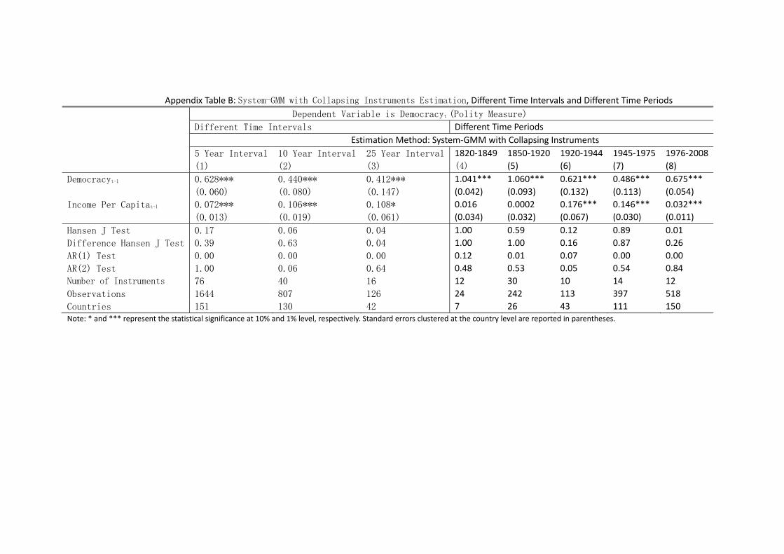
measurement. Thus far, we have used the data employed by AJRY (2008),which cover the 1950-2000 period. As more data have since become available,we �rst extend the sample period to 2010. Speci�cally, we obtain data onincome per capita from Penn World Table 7.011 and on democracy fromFreedom House.12 This enables us to include more countries in the analysis,yielding an increase of 47 countries in the system-GMM estimation. Thisallows us to make sure our earlier results are not driven by the particularsample period and the particular set of countries examined. It is reassuringto �nd that income per capita continues to have a positive and statisticallysigni�cant impact on democracy in the system-GMM estimation (Column 8of Table 4).Second, using the Polity IV measure of democracy enables us to further

extend the �rst year of the sample period from 1950 to 1820, while dataon income per capita from 1820 to 1950 are obtained from the study ofMaddison (2010).13 In Column 1 of Table 5, we report the system-GMMestimation results for the 1820-2008 sample period using a 5-year interval

10For the rationales of these two instruments, please refer to the original paper of AJRY(2008).11Web site: http://pwt.econ.upenn.edu/php_site/pwt_index.php12Web site: http://www.freedomhouse.org/13Web site: http://www.ggdc.net/MADDISON/oriindex.htm

10

as in our main analysis. Clearly, the results are qualitatively the same asthose reported earlier, implying our results are robust for the longer sampleperiod. Moreover, in Columns 2-3 of Table 5, we investigate the impact ofincome per capita on democracy using longer time intervals of 10 and 25years, respectively. The coe¢ cient of income per capita remains positive andstatistically signi�cant. Our results lend further support to Boix (2011), whohighlights the importance of including the earlier waves of democratizationin investigating the impact of income per capita on democracy.14 Moreover,the coe¢ cients are much larger than those obtained in the shorter time inter-val (i.e., the �ve-year interval), presumably because greater changes can bedetected over longer time intervals of variable measurement, similar to whatTreisman (2011) reports.Di¤erent time periods. As noted by Boix (2011), democratization has

occurred in waves over the last 200 years. It is therefore possible that theimpact of income per capita on democracy may di¤er in di¤erent time peri-ods. To examine this possibility, we divide our sample into �ve time periods�1820-1849 (pre-�rst wave of democracy), 1850-1920 (�rst wave), 1920-1944(reversal), 1945-1975 (second wave and reversal), and 1976-2008 (third waveof democratization) �in a manner similar to Boix (2011). The system-GMMestimation results are summarized in Table 6. It is clear that other thanduring the �rst time period (1820-1849), the coe¢ cient of income per capitaon democracy is always positive and statistically signi�cant, consistent withour aforementioned main results.15

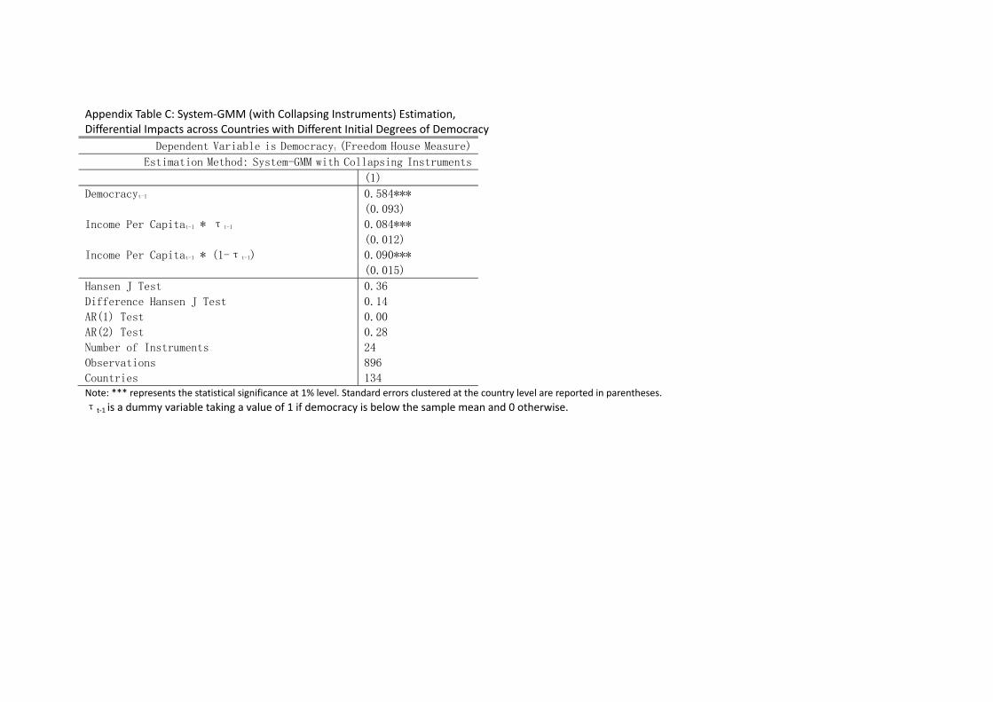
Di¤erential impacts across countries with di¤erent initial de-grees of democracy. There is a debate regarding whether the impact ofincome per capita on democracy may depend on the initial degree of democ-racy (see, for example, Przeworski and Limongi, 1997; Przeworski, Alvarez,Cheibub and Limongi, 2000; Boix and Stokes, 2003). Speci�cally, for a coun-try with a low initial degree of democracy, an increase in income per capitamay facilitate its transition to democracy (called the endogenous theory inthe literature). Meanwhile, for a country with a high initial degree of democ-racy, an increase in income per capita may make it less likely to revert todictatorship (called the exogenous theory in the literature).To investigate the validity of these two theories, we modify (1) as follows

(i.e., in the same manner as AJRY (2009))

14Boix (2011) points out that few countries had democratic systems in the �rst half ofthe nineteenth century, and including this period in the statistical analysis is crucial torevealing the impact of income per capita on democracy.15The coe¢ cient of income per capita for the �rst period is also positive, but insigni�-

cant, presumably because of the small sample size (i.e., 24 observations).

11

dit = �dit�1 + ENDO� it�1yit�1 +

EXO(1� � it�1)yit�1 + �t + �i + "it (5)

where � it�1 is a dummy variable equal to 1 if dit�1 is below the sample meanand 0 otherwise; ENDO captures the e¤ect of income per capita on democ-racy for countries in which the degree of democracy is below the sample mean(the exogenous theory); and EXO captures the e¤ect of income per capitaon democracy for countries in which the degree of democracy is above thesample mean (the endogenous theory). The system-GMM estimation resultsare reported in Table 7. It is found that EXO is positive and statisticallysigni�cant, supporting the exogenous theory and consistent with the �ndingsof Przeworski and Limongi (1997) and Boix and Stokes (2003). Meanwhile, ENDO is also positive and statistically signi�cant, supporting the endogenoustheory and consistent with the �ndings of Boix and Stokes (2003). Moreover,these results are consistent with our aforementioned results, but are in sharpcontrast to those reported by AJRY (2009).Collapsed system-GMM. Recall that in the main analysis (Section

3.1) we use collapsing instruments as a check of the validity of the system-GMM estimation. Here, we conduct a similar analysis for all the aboverobustness checks and �nd that our results are qualitatively the same. Fordetails, see Tables A, B, and C of the Appendix.It is interesting to note that there are certain cases where the speci�cation

tests (i.e., the Hansen J test and the di¤erence Hansen J test) fail. However,these are also the cases where the di¤erence-GMM estimations also fail thespeci�cation test (i.e., the Hansen J test). Moreover, the estimated coe¢ cientof income per capita obtained using the system-GMM estimation with thefull instrument set is qualitatively the same as those obtained using collapsinginstruments. These results suggest that our system-GMM estimation resultsare not a¤ected by the instrument proliferation problem.

4 Conclusion

The seminal work of AJRY (2008) on the unimportance of income per capitato democracy has caused quite a stir in the economics and political sci-ence community. The identi�cation of AJRY (2008) relies on the use of thedi¤erence-GMM method; however, this method su¤ers from the weak instru-ment problem when the dependent variable (i.e., the degree of democracy)is highly persistent over time. In this paper, we revisit the impact of incomeper capita on democracy using the system-GMMmethod, which is developedto correct the weak instrument problem encountered by the di¤erence-GMM

12

method. Using the same data set as that employed by AJRY (2008), we�nd that income per capita has a positive and highly signi�cant impact ondemocracy, thus reversing their results. Given that it is impossible to conducta controlled experiment on this topic, studies have to rely on the examina-tion of non-randomized, secondary data with somewhat imperfect estimationmethodologies. Nonetheless, the results we obtain using the system-GMMmethod �a method arguably better than its di¤erence-GMM alternative fordealing with the potential endogeneity problem in panel data �add moreweight for acceptance of the modernization theory, i.e., that economic devel-opment promotes democracy.

References

[1] Acemoglu, Daron, Simon Johnson, James A. Robinson, and PierreYared. 2008. Income and Democracy.American Economic Review, 98(3):808-842.

[2] Acemoglu, Daron, Simon Johnson, James A. Robinson, and PierreYared. 2009. Reevaluating the Modernization Hypothesis. Journal ofMonetary Economics, 56(8): 1043-1058.

[3] Andersen, Torben G. and Bent E. Sorensen. 1996. GMM Estimation of aStochastic Volatility Model: a Monte Carlo Study. Journal of Businessand Economic Statistics, 14(3): 328-352.

[4] Arellano, Manuel and Stephen Bond. 1991. Some Tests of Speci�cationfor Panel Data: Monte Carlo Evidence and An Application to Employ-ment Equations. Review of Economic Studies, 58(2): 277-297.

[5] Arellano, Manuel and Olympia Bover. 1995. Another Look at the In-strumental Variable Estimation of Error-components Models. Journalof Econometrics, 68: 29-51.

[6] Aslaksen, Silje. 2010. Oil and Democracy: More than a Cross-CountryCorrelation? Journal of Peace Research, 47(4): 421-431.

[7] Barro, Robert J. 1997. Determinants of Economic Growth: A Cross-Country Empirical Study. Cambridge: MIT Press.

[8] Barro, Robert J. 1999. Determinants of Democracy. Journal of PoliticalEconomy, 107: 158-183.

13

[9] Benhabib, Jess, Alejandro Corvalan, and Mark M. Spiegel. 2011.Reestablishing the Income-democracy Nexus. NBER Working Paper16832.

[10] Blundell, Richard and Stephen Bond. 1998. Initial Conditions and Mo-ment Restrictions in Dynamic Panel Data Models. Journal of Econo-metrics, 87: 115-143.

[11] Blundell, Richard and Stephen Bond. 2000. GMM Estimation with Per-sistent Panel Data: an Application to Production Functions. Economet-ric Review, 19(3): 321-340.

[12] Bobba, Matteo and Decio Coviello. 2007. Weak Instruments and WeakIdenti�cation, in Estimating the E¤ects of Education, on Democracy.Economic Letters, 96: 301-306.

[13] Boix, Carles and Susan C. Stokes. 2003. Endogenous Democratization.World Politics, 55(4): 517-549.

[14] Boix, Carles. 2011. Democracy, Development, and the International Sys-tem. American Political Science Review, 105(4): 809-828.

[15] Bond, Stephen R. 2002. Dynamic Panel Data Models: a Guide to MicroData Methods and Practice. Portuguese Economic Journal, 1: 141-162.

[16] Bowsher, Clive G. 2002. On Testing Overidentifying Restrictions in Dy-namic Panel Data Models, Economics Letters, 77: 211-220.

[17] Castello-Climent, Amparo. 2008. On the Distribution of Education andDemocracy. Journal of Development Economics, 87: 179-190.

[18] Glaeser, Edward L., Rafael La Porta, Florencio Lopez-De-Silanes, andAndrei Shleifer. 2004. Do Institutions Cause Growth? Journal of Eco-nomic Growth, 9: 271-303.

[19] Glaeser, Edward L., Giacomo A.M. Ponzetto, and Andrei Shleifer. 2007.Why Does Democracy Need Education? Journal of Economic Growth,12: 77-99.

[20] Holtz-Eakin, Douglas, Whitney Newey, and Harvey S. Rosen. 1988. Es-timating Vector Autoregressions with Panel Data. Econometrica, 56(6):1371-1395.

14

[21] Lipset, Seymour Martin. 1959. Some Social Requisites of Democracy:Economic development and Political Legitimacy. American Political Sci-ence Review, 53(1): 69-105.

[22] Maddison, Angus. 2010. Statistics on World Population, GDP and PerCapita GDP, 1-2008 AD.

[23] Miller, Michael K. Forthcoming. Economic Development, Violent LeaderRemoval, and Democratization. American Journal of Political Science.

[24] Papaioannou, Elias and Gregorios Siourounis. 2008. Economic and So-cial Factors Driving the Third Wave of Democratization. Journal ofComparative Economics, 36: 365-387.

[25] Przeworski, Adam and Fernando Limongi. 1997. Modernization: Theo-ries and Facts. World Politics, 49(2): 155-183.

[26] Przeworski, Adam, Michael E. Alvarez, Jose Antonio Cheibub, and Fer-nando Limongi. 2000. Democracy and Development: Political Institu-tions and Well-being in the World, 1950-1990. Cambridge: CambridgeUniversity Press.

[27] Roodman, David. 2009a. How to Do Xtabond2: an Introduction to Dif-ference and System GMM in Stata. Stata Journal, 9(1): 86-136.

[28] Roodman, David. 2009b. A Note on the Theme of Too Many Instru-ments. Oxford Bulletin of Economics and Statistics, 71(1): 0305-9049.

[29] Staiger, Douglas and James H. Stock. 1997. Instrumental variables re-gression with weak instruments. Econometrica, 65(3): 557-586.

[30] Stock, James H. and Jonathan H. Wright. 2000. GMM with Weak Iden-ti�cation. Econometrica, 68(5): 1055-1096.

[31] Stock, James H., Jonathan H. Wright and Motohiro Yogo. 2002. A Sur-vey of Weak Instruments andWeak Identi�cation in Generalized Methodof Moments. Journal of Business and Economic Statistics, 20(4): 518-529.

[32] Treisman, Daniel. 2011. Income, Democracy, and the Cunning of Rea-son. NBER Working Paper 17132.

[33] Windmeijer, Frank. 2005. A Finite Sample Correction for the Varianceof Linear E¢ cient Two-step GMMEstimators. Journal of Econometrics,126: 25-51.

15

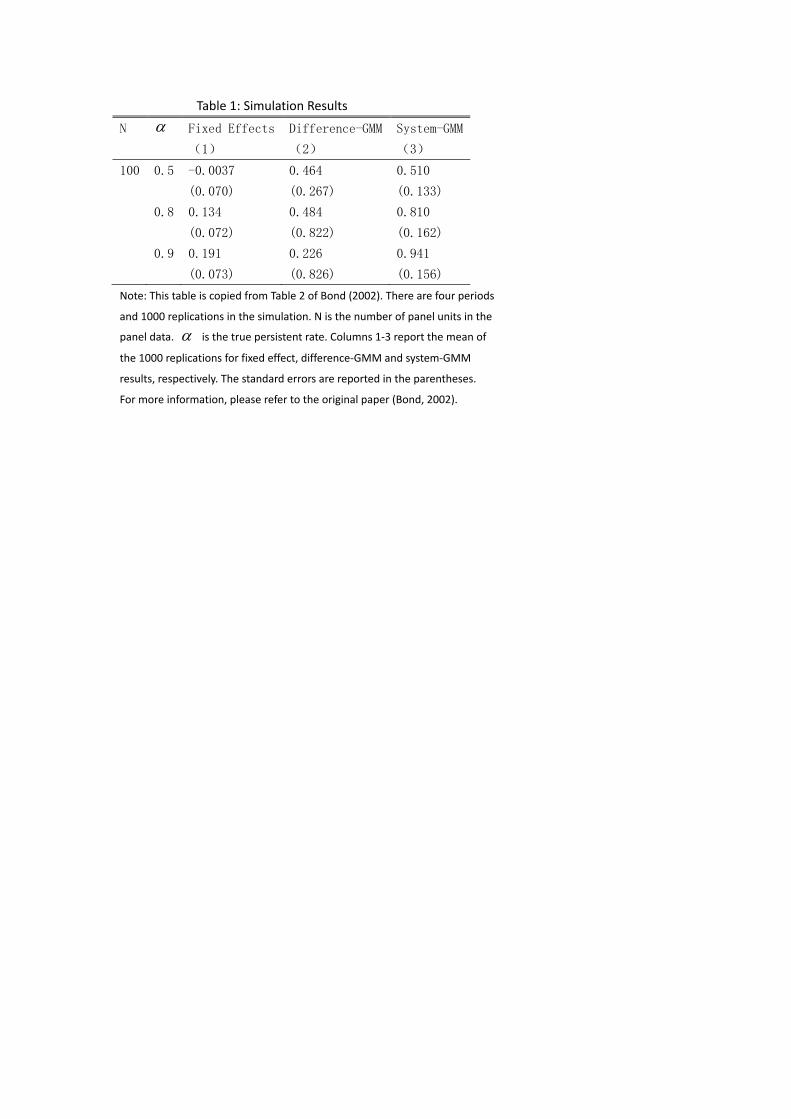
Table 1: Simulation Results

N Fixed Effects

（1）

Difference-GMM

（2）

System-GMM

（3）

100 0.5 -0.0037 0.464 0.510

(0.070) (0.267) (0.133)

0.8 0.134 0.484 0.810

(0.072) (0.822) (0.162)

0.9 0.191 0.226 0.941

(0.073) (0.826) (0.156)

Note: This table is copied from Table 2 of Bond (2002). There are four periods

and 1000 replications in the simulation. N is the number of panel units in the

panel data. is the true persistent rate. Columns 1‐3 report the mean of

the 1000 replications for fixed effect, difference‐GMM and system‐GMM

results, respectively. The standard errors are reported in the parentheses.

For more information, please refer to the original paper (Bond, 2002).

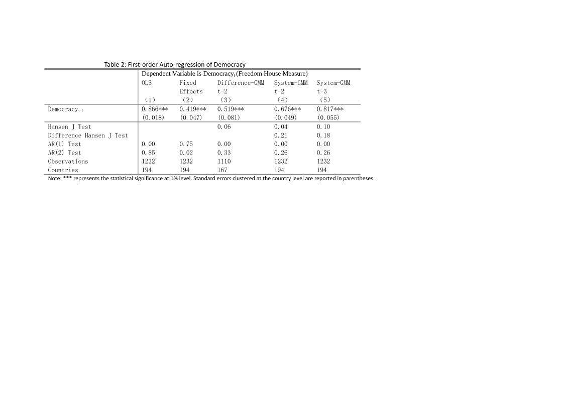
Table 2: First‐order Auto‐regression of Democracy

Dependent Variable is Democracyt (Freedom House Measure) OLS

（1）

Fixed

Effects

（2）

Difference-GMM

t-2

（3）

System-GMM

t-2

（4）

System-GMM

t-3

（5）

Democracyt-1 0.866*** 0.419*** 0.519*** 0.676*** 0.817***

(0.018) (0.047) (0.081) (0.049) (0.055)

Hansen J Test 0.06 0.04 0.10

Difference Hansen J Test 0.21 0.18

AR(1) Test 0.00 0.75 0.00 0.00 0.00

AR(2) Test 0.85 0.02 0.33 0.26 0.26

Observations 1232 1232 1110 1232 1232

Countries 194 194 167 194 194 Note: *** represents the statistical significance at 1% level. Standard errors clustered at the country level are reported in parentheses.

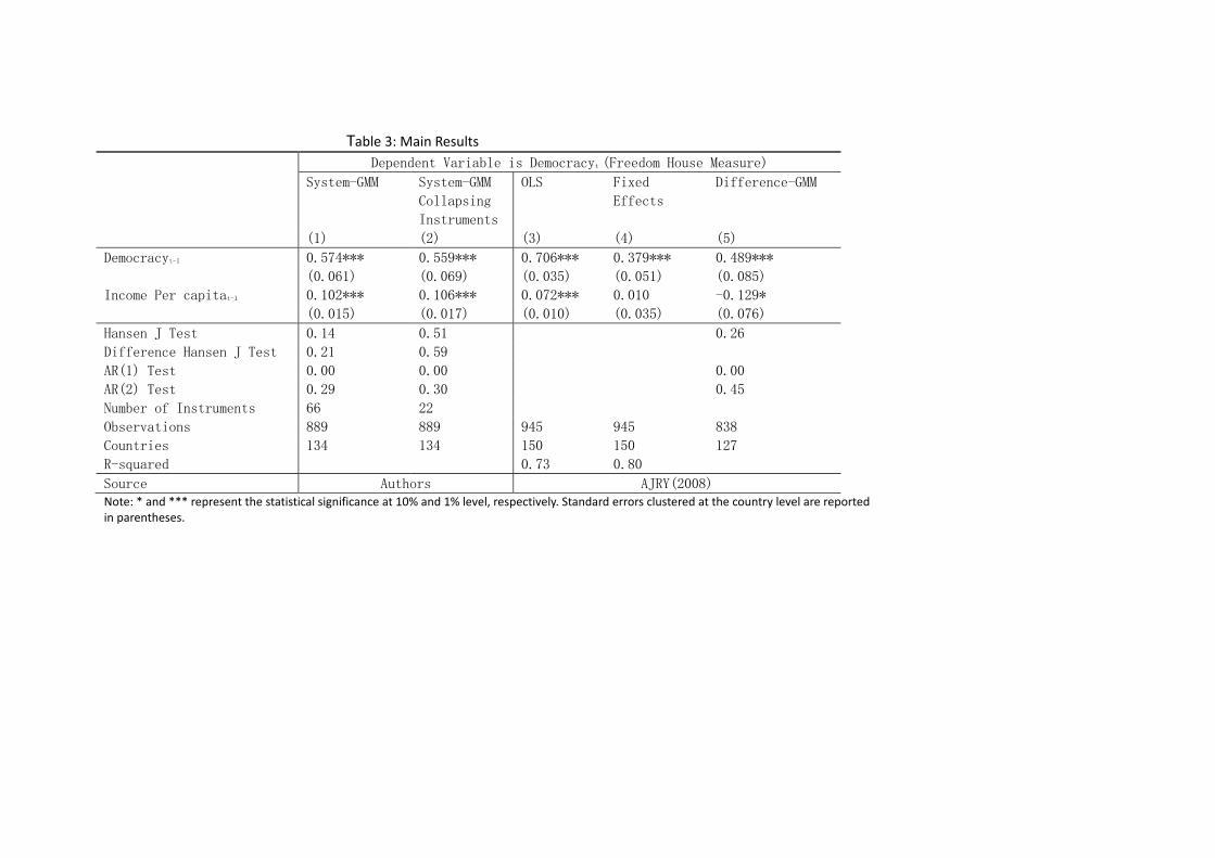
Table 3: Main Results

Dependent Variable is Democracyt (Freedom House Measure)

System-GMM

System-GMM

Collapsing

Instruments

OLS

Fixed

Effects

Difference-GMM

(1) (2) (3) (4) (5)

Democracyt-1 0.574*** 0.559*** 0.706*** 0.379*** 0.489***

(0.061) (0.069) (0.035) (0.051) (0.085)

Income Per capitat-1 0.102*** 0.106*** 0.072*** 0.010 -0.129*

(0.015) (0.017) (0.010) (0.035) (0.076)

Hansen J Test 0.14 0.51 0.26

Difference Hansen J Test 0.21 0.59

AR(1) Test 0.00 0.00 0.00

AR(2) Test 0.29 0.30 0.45

Number of Instruments 66 22

Observations 889 889 945 945 838

Countries 134 134 150 150 127

R-squared 0.73 0.80

Source Authors AJRY(2008) Note: * and *** represent the statistical significance at 10% and 1% level, respectively. Standard errors clustered at the country level are reported in parentheses.

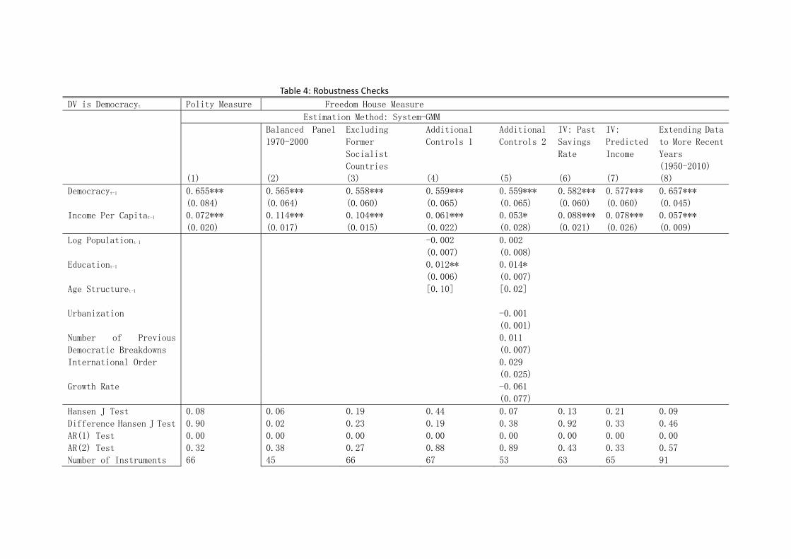
Table 4: Robustness Checks

DV is Democracyt Polity Measure Freedom House Measure

Estimation Method: System-GMM

Balanced Panel

1970-2000

Excluding

Former

Socialist

Countries

Additional

Controls 1

Additional

Controls 2

IV: Past

Savings

Rate

IV:

Predicted

Income

Extending Data

to More Recent

Years

(1950-2010)

(1) (2) (3) (4) (5) (6) (7) (8)

Democracyt-1 0.655*** 0.565*** 0.558*** 0.559*** 0.559*** 0.582*** 0.577*** 0.657***

(0.084) (0.064) (0.060) (0.065) (0.065) (0.060) (0.060) (0.045)

Income Per Capitat-1 0.072*** 0.114*** 0.104*** 0.061*** 0.053* 0.088*** 0.078*** 0.057***

(0.020) (0.017) (0.015) (0.022) (0.028) (0.021) (0.026) (0.009)

Log Populationt-1 -0.002 0.002

(0.007) (0.008)

Educationt-1 0.012** 0.014*

(0.006) (0.007)

Age Structuret-1 [0.10] [0.02]

Urbanization -0.001

(0.001)

Number of Previous

Democratic Breakdowns

0.011

(0.007)

International Order 0.029

(0.025)

Growth Rate -0.061

(0.077)

Hansen J Test 0.08 0.06 0.19 0.44 0.07 0.13 0.21 0.09

Difference Hansen J Test 0.90 0.02 0.23 0.19 0.38 0.92 0.33 0.46

AR(1) Test 0.00 0.00 0.00 0.00 0.00 0.00 0.00 0.00

AR(2) Test 0.32 0.38 0.27 0.88 0.89 0.43 0.33 0.57

Number of Instruments 66 45 66 67 53 63 65 91

Observations 802 567 868 662 521 891 895 1403

Countries 121 81 125 94 82 134 124 181 Note: *, **, *** represent the statistical significance at 10%, 5%, 1% level, respectively. Standard errors clustered at the country level are reported in parentheses. DV denotes dependent variable.

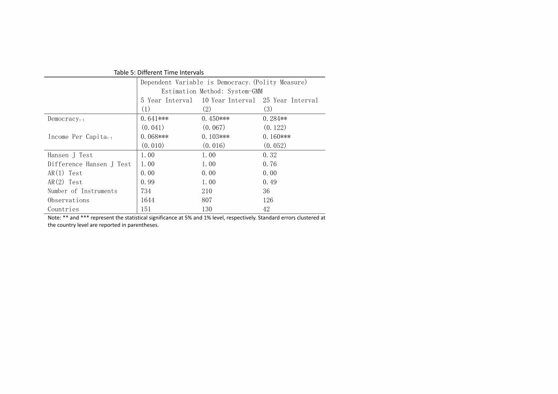
Table 5: Different Time Intervals

Dependent Variable is Democracyt (Polity Measure)


5 Year Interval 10 Year Interval 25 Year Interval

(1) (2) (3)

Democracyt-1 0.641*** 0.450*** 0.284**

(0.041) (0.067) (0.122)

Income Per Capitat-1 0.068*** 0.103*** 0.160***

(0.010) (0.016) (0.052)

Hansen J Test 1.00 1.00 0.32

Difference Hansen J Test 1.00 1.00 0.76

AR(1) Test 0.00 0.00 0.00

AR(2) Test 0.99 1.00 0.49

Number of Instruments 734 210 36

Observations 1644 807 126

Countries 151 130 42 Note: ** and *** represent the statistical significance at 5% and 1% level, respectively. Standard errors clustered at the country level are reported in parentheses.

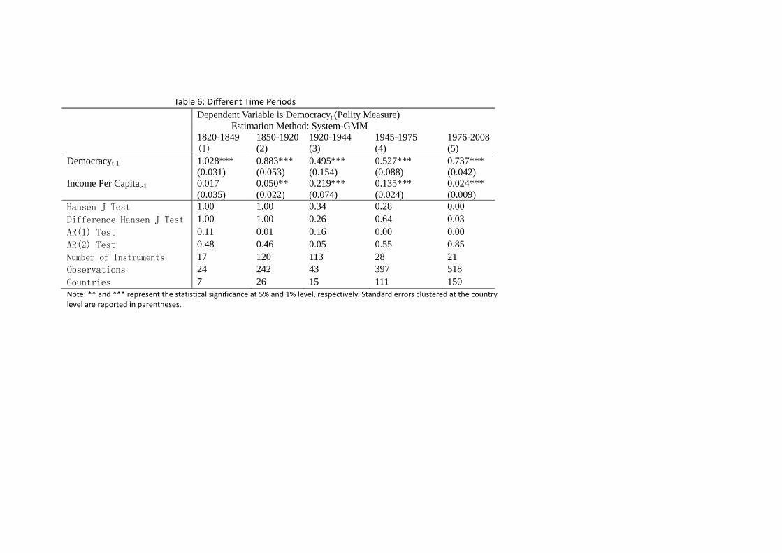
Table 6: Different Time Periods

Dependent Variable is Democracyt (Polity Measure) Estimation Method: System-GMM 1820-1849 1850-1920 1920-1944 1945-1975 1976-2008 (1) (2) (3) (4) (5) Democracyt-1 1.028*** 0.883*** 0.495*** 0.527*** 0.737*** (0.031) (0.053) (0.154) (0.088) (0.042) Income Per Capitat-1 0.017 0.050** 0.219*** 0.135*** 0.024*** (0.035) (0.022) (0.074) (0.024) (0.009) Hansen J Test 1.00 1.00 0.34 0.28 0.00 Difference Hansen J Test 1.00 1.00 0.26 0.64 0.03 AR(1) Test 0.11 0.01 0.16 0.00 0.00 AR(2) Test 0.48 0.46 0.05 0.55 0.85 Number of Instruments 17 120 113 28 21 Observations 24 242 43 397 518 Countries 7 26 15 111 150 Note: ** and *** represent the statistical significance at 5% and 1% level, respectively. Standard errors clustered at the country level are reported in parentheses.

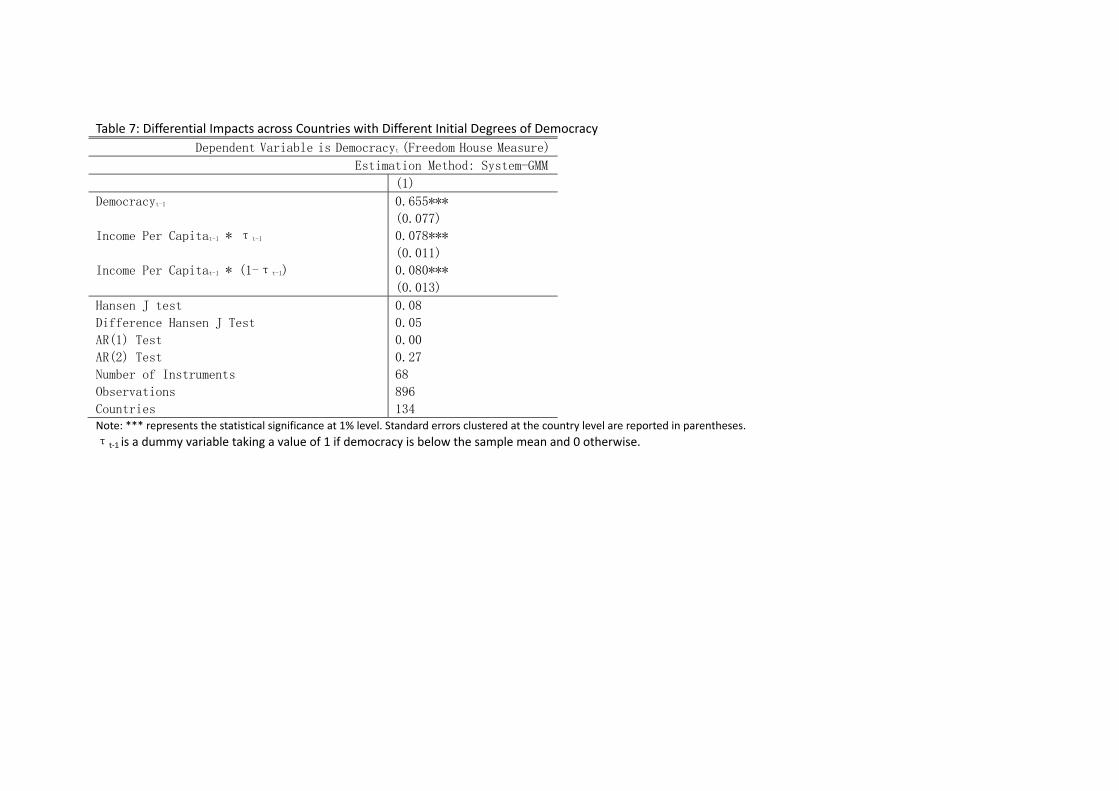
Table 7: Differential Impacts across Countries with Different Initial Degrees of Democracy



(1)

Democracyt-1 0.655***

(0.077)

Income Per Capitat-1 * τt-1 0.078***

(0.011)

Income Per Capitat-1 * (1-τt-1) 0.080***

(0.013)

Hansen J test 0.08

Difference Hansen J Test 0.05

AR(1) Test 0.00

AR(2) Test 0.27

Number of Instruments 68

Observations 896

Countries 134 Note: *** represents the statistical significance at 1% level. Standard errors clustered at the country level are reported in parentheses.

τt‐1 is a dummy variable taking a value of 1 if democracy is below the sample mean and 0 otherwise.

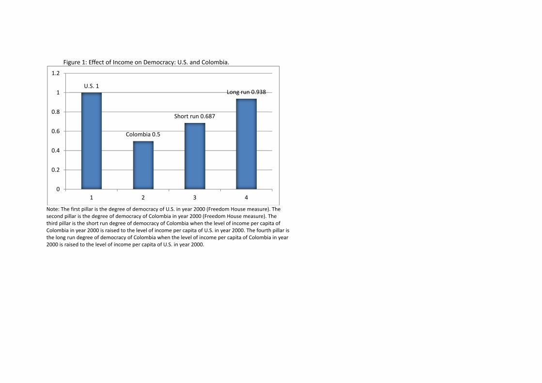
Figure 1: Effect of Income on Democracy: U.S. and Colombia.

Note: The first pillar is the degree of democracy of U.S. in year 2000 (Freedom House measure). The second pillar is the degree of democracy of Colombia in year 2000 (Freedom House measure). The third pillar is the short run degree of democracy of Colombia when the level of income per capita of Colombia in year 2000 is raised to the level of income per capita of U.S. in year 2000. The fourth pillar is the long run degree of democracy of Colombia when the level of income per capita of Colombia in year 2000 is raised to the level of income per capita of U.S. in year 2000.

U.S. 1

Colombia 0.5

Short run 0.687

Long run 0.938

0

0.2

0.4

0.6

0.8

1

1.2

1 2 3 4

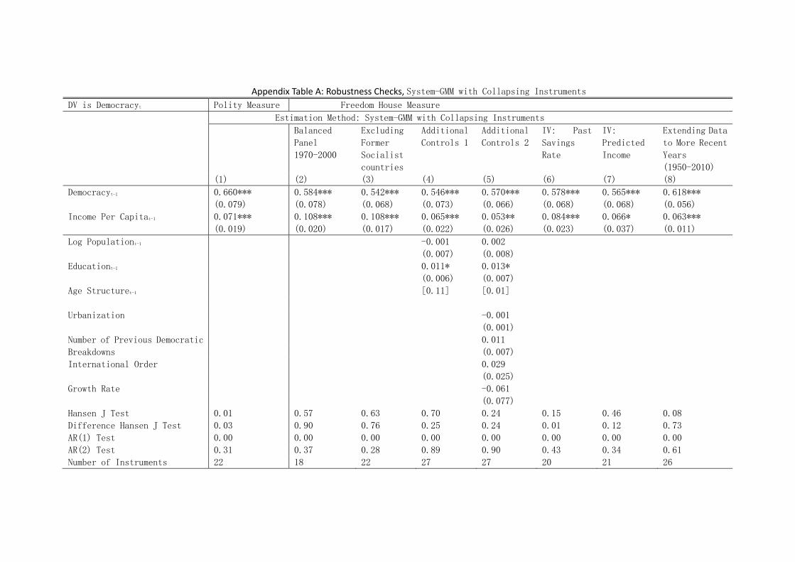
Appendix Table A: Robustness Checks, System-GMM with Collapsing Instruments

DV is Democracyt Polity Measure Freedom House Measure

Estimation Method: System-GMM with Collapsing Instruments

Balanced

Panel

1970-2000

Excluding

Former

Socialist

countries

Additional

Controls 1

Additional

Controls 2

IV: Past

Savings

Rate

IV:

Predicted

Income

Extending Data

to More Recent

Years

(1950-2010)

(1) (2) (3) (4) (5) (6) (7) (8)

Democracyt-1 0.660*** 0.584*** 0.542*** 0.546*** 0.570*** 0.578*** 0.565*** 0.618***

(0.079) (0.078) (0.068) (0.073) (0.066) (0.068) (0.068) (0.056)

Income Per Capitat-1 0.071*** 0.108*** 0.108*** 0.065*** 0.053** 0.084*** 0.066* 0.063***

(0.019) (0.020) (0.017) (0.022) (0.026) (0.023) (0.037) (0.011)

Log Populationt-1 -0.001 0.002

(0.007) (0.008)

Educationt-1 0.011* 0.013*

(0.006) (0.007)

Age Structuret-1 [0.11] [0.01]

Urbanization -0.001

(0.001)

Number of Previous Democratic

Breakdowns

0.011

(0.007)

International Order 0.029

(0.025)

Growth Rate -0.061

(0.077)

Hansen J Test 0.01 0.57 0.63 0.70 0.24 0.15 0.46 0.08


AR(1) Test 0.00 0.00 0.00 0.00 0.00 0.00 0.00 0.00

AR(2) Test 0.31 0.37 0.28 0.89 0.90 0.43 0.34 0.61


Observations 802 567 868 662 521 891 895 1403

Countries 121 81 125 94 82 134 124 181 Note: *, **, *** represent the statistical significance at 10%, 5%, 1% level, respectively. Standard errors clustered at the country level are reported in parentheses. DV denotes dependent variable.

Appendix Table B: System-GMM with Collapsing Instruments Estimation, Different Time Intervals and Different Time Periods

Dependent Variable is Democracyt (Polity Measure)

Different Time Intervals Different Time Periods

Estimation Method: System‐GMM with Collapsing Instruments

5 Year Interval 10 Year Interval 25 Year Interval 1820‐1849 1850‐1920 1920‐1944 1945‐1975 1976‐2008

(1) (2) (3) (4) (5) (6) (7) (8)

Democracyt-1 0.628*** 0.440*** 0.412*** 1.041*** 1.060*** 0.621*** 0.486*** 0.675***

(0.060) (0.080) (0.147) (0.042) (0.093) (0.132) (0.113) (0.054)

Income Per Capitat-1 0.072*** 0.106*** 0.108* 0.016 0.0002 0.176*** 0.146*** 0.032***

(0.013) (0.019) (0.061) (0.034) (0.032) (0.067) (0.030) (0.011)

Hansen J Test 0.17 0.06 0.04 1.00 0.59 0.12 0.89 0.01


AR(1) Test 0.00 0.00 0.00 0.12 0.01 0.07 0.00 0.00

AR(2) Test 1.00 0.06 0.64 0.48 0.53 0.05 0.54 0.84


Observations 1644 807 126 24 242 113 397 518

Countries 151 130 42 7 26 43 111 150Note: * and *** represent the statistical significance at 10% and 1% level, respectively. Standard errors clustered at the country level are reported in parentheses.

Appendix Table C: System‐GMM (with Collapsing Instruments) Estimation, Differential Impacts across Countries with Different Initial Degrees of Democracy


Estimation Method: System-GMM with Collapsing Instruments

(1)

Democracyt-1 0.584***

(0.093)

Income Per Capitat-1 * τt-1 0.084***

(0.012)

Income Per Capitat-1 * (1-τt-1) 0.090***

(0.015)

Hansen J Test 0.36

Difference Hansen J Test 0.14

AR(1) Test 0.00

AR(2) Test 0.28

Number of Instruments 24

Observations 896

Countries 134 Note: *** represents the statistical significance at 1% level. Standard errors clustered at the country level are reported in parentheses.

τt‐1 is a dummy variable taking a value of 1 if democracy is below the sample mean and 0 otherwise.

Documents

The Impact of Income on Democracy Revisited