Globalization and income inequality - revisitedec.europa.eu/economy_finance/events/2016/20161128-arc2016/... · Globalization and income inequality - revisited - ... MNG MWI MYS NAM

Globalization and income inequality- revisited -

Florian Dorn1,2 Clemens Fuest1,2 Niklas Potrafke1,2

1Ifo Institute, Munich

2University of Munich (LMU)

DG ECFIN Fellowship Initiative 2016/17Annual Research Conference - Brusells, 28th November 2016

Theoretical predictions

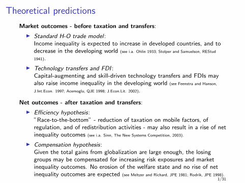
Market outcomes - before taxation and transfers:

I Standard H-O trade model :Income inequality is expected to increase in developed countries, and todecrease in the developing world (see i.a. Ohlin 1933; Stolper and Samuelson, REStud

1941).

I Technology transfers and FDI :Capital-augmenting and skill-driven technology transfers and FDIs mayalso raise income inequality in the developing world (see Feenstra and Hanson,

J.Int.Econ. 1997; Acemoglu, QJE 1998; J.Econ.Lit. 2002).

Net outcomes - after taxation and transfers:

I Efficiency hypothesis:”Race-to-the-bottom” - reduction of taxation on mobile factors, ofregulation, and of redistribution activities - may also result in a rise of netinequality outcomes (see i.a. Sinn, The New Systems Competition, 2003).

I Compensation hypothesis:Given the total gains from globalization are large enough, the losinggroups may be compensated for increasing risk exposures and marketinequality outcomes. No erosion of the welfare state and no rise of netinequality outcomes are expected (see Meltzer and Richard, JPE 1981; Rodrik, JPE 1998).

1/31

Current state of empirical research

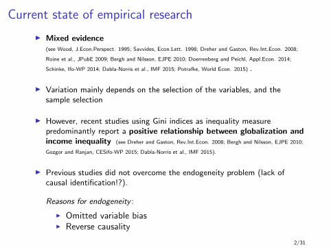
I Mixed evidence(see Wood, J.Econ.Perspect. 1995; Savvides, Econ.Lett. 1998; Dreher and Gaston, Rev.Int.Econ. 2008;

Roine et al., JPubE 2009; Bergh and Nilsson, EJPE 2010; Doerrenberg and Peichl, Appl.Econ. 2014;

Schinke, Ifo-WP 2014; Dabla-Norris et al., IMF 2015; Potrafke, World Econ. 2015) .

I Variation mainly depends on the selection of the variables, and thesample selection

I However, recent studies using Gini indices as inequality measurepredominantly report a positive relationship between globalization andincome inequality (see Dreher and Gaston, Rev.Int.Econ. 2008; Bergh and Nilsson, EJPE 2010;

Gozgor and Ranjan, CESifo-WP 2015; Dabla-Norris et al., IMF 2015).

I Previous studies did not overcome the endogeneity problem (lack ofcausal identification!?).

Reasons for endogeneity :

I Omitted variable biasI Reverse causality

2/31

Our results and contribution

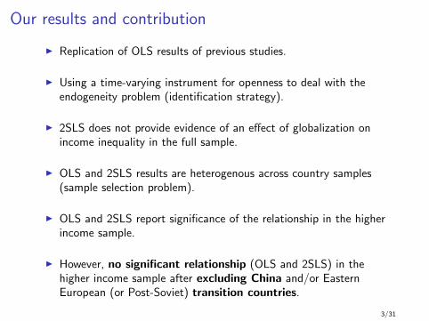
I Replication of OLS results of previous studies.

I Using a time-varying instrument for openness to deal with theendogeneity problem (identification strategy).

I 2SLS does not provide evidence of an effect of globalization onincome inequality in the full sample.

I OLS and 2SLS results are heterogenous across country samples(sample selection problem).

I OLS and 2SLS report significance of the relationship in the higherincome sample.

I However, no significant relationship (OLS and 2SLS) in thehigher income sample after excluding China and/or EasternEuropean (or Post-Soviet) transition countries.

3/31

Outline

1. Theory and related literature

2. Data and Descriptives

3. OLS fixed effects

4. IV strategy and 2SLS

5. Results by economic development levels

6. The role of transition countries

7. Summary and outlook

4/31

2. Data and descriptives

5/31

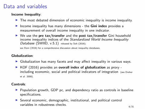
Data and variables

Income Inequality:

I The most debated dimension of economic inequality is income inequality.

I Income inequality has many dimensions - the Gini index provides ameasurement of overall income inequality in one indicator.

I We use the pre tax/transfer and the post tax/transfer Gini householdincome inequality indices of the Standardized World Income InequalityDatabase (SWIID, v.5.1) released by Solt (2016);

see Dorn (2016) for a comprehensive discussion about inequality databases.

Globalization:

I Globalization has many facets and may affect inequality in various ways.

I KOF (2016) provides an overall index of globalization as proxy -including economic, social and political indicators of integration (see Dreher

et al. 2008).

Controls:

I Population growth, GDP pc, and dependency ratio as controls in baselinespecifications.

I Several economic, demographic, institutional, and political controlvariables in robustness checks.

6/31

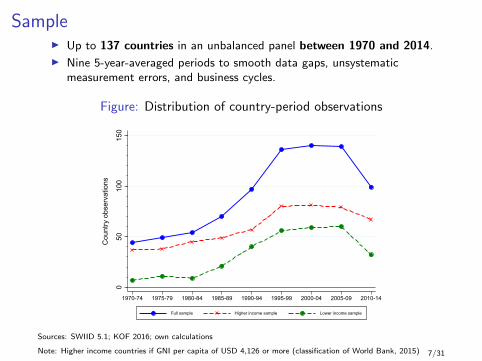
SampleI Up to 137 countries in an unbalanced panel between 1970 and 2014.

I Nine 5-year-averaged periods to smooth data gaps, unsystematicmeasurement errors, and business cycles.

Figure: Distribution of country-period observations0

5010

015

0

Cou

ntry

obs

erva

tions

1970-74 1975-79 1980-84 1985-89 1990-94 1995-99 2000-04 2005-09 2010-14

Full sample Higher income sample Lower income sample

Sources: SWIID 5.1; KOF 2016; own calculations

Note: Higher income countries if GNI per capita of USD 4,126 or more (classification of World Bank, 2015) 7/31

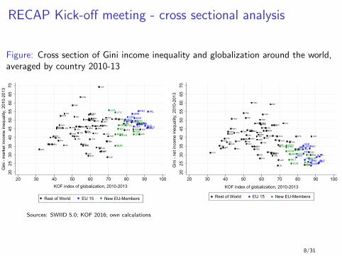
RECAP Kick-off meeting - cross sectional analysis

Figure: Cross section of Gini income inequality and globalization around the world,averaged by country 2010-13

AFG

ARG

ARM

AUS

BGD

BLR

BOL

BRA

BRB

BTN

CAN

CHE

CHLCHNCOL CRI

DOMECU

ETH

GEO

GTM

HND

IDN

IND

IRN

ISL

ISR

JOR

JPN

KAZ

KGZ

KOR

LKA

MDA

MDG

MDV

MEXMKD

MLI

MNE

MNG

MWI

MYS

NAM

NGANOR

NPL

NZL

PAK

PAN

PERPHL

PRI

PRYRUS

RWA

SEN

SGP

SLE

SLV

SRB

TGOTHA

TUNTUR

TZA

UGA

UKR

URYUSA

VEN

VNM

ZAF

ZMB

ZWEAUT

BEL

DEUDNK

ESP

FINFRA

GBRGRC

IRL

ITA

LUX NLD

PRT

SWE

BGR

CYP

CZE

ESTHRV

HUN

LTULVA

MLTPOL

ROM SVKSVN

2025

3035

4045

5055

6065

70G

ini -

mar

ket i

ncom

e in

equa

lity,

201

0-20

13

20 30 40 50 60 70 80 90 100KOF index of globalization, 2010-2013

Rest of World EU 15 New EU-Members

AFG

ARG

ARMAUS

BGD

BLR

BOL

BRA

BRB

BTN

CAN

CHE

CHL

CHN

COL

CRIDOMECU

ETH

GEO

GTM

HND

IDN

IND

IRN

ISL

ISR

JOR

JPNKAZ

KGZ

KOR

LKA

MDA

MDG

MDV

MEX

MKD

MLI

MNE

MNG

MWI

MYS

NAM

NGA

NOR

NPLNZL

PAK

PANPER

PHL

PRI

PRY

RUS

RWA

SENSGP

SLE

SLV

SRB

TGO THATUN

TUR

TZA

UGA

UKR

URY

USAVEN

VNM

ZAF

ZMB

ZWE

AUT

BEL

DEU

DNK

ESP

FIN

FRA

GBRGRC

IRL

ITA

LUXNLD

PRT

SWE

BGR

CYP

CZE

ESTHRV

HUN

LTULVA

MLT

POLROM

SVKSVN

2025

3035

4045

5055

6065

70G

ini -

net

inco

me

ineq

ualit

y, 2

010-

2013

20 30 40 50 60 70 80 90 100

KOF index of globalization, 2010-2013

Rest of World EU 15 New EU-Members

Sources: SWIID 5.0; KOF 2016; own calculations

8/31

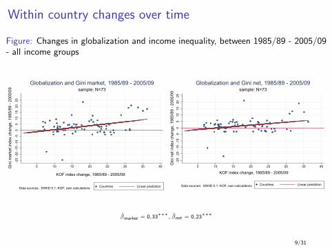
Within country changes over time

Figure: Changes in globalization and income inequality, between 1985/89 - 2005/09- all income groups

-25

-20

-15

-10

-50

510

1520

25

Gin

i mar

ket i

ndex

cha

nge,

198

5/89

- 20

05/0

9

5 10 15 20 25 30 35 40

KOF index change, 1985/89 - 2005/09

Countries Linear predictionData sources: SWIID 5.1; KOF; own calculations

sample: N=73Globalization and Gini market, 1985/89 - 2005/09

-25

-20

-15

-10

-50

510

1520

25G

ini n

et in

dex

chan

ge, 1

985/

89 -

2005

/09

5 10 15 20 25 30 35 40



sample: N=73Globalization and Gini net, 1985/89 - 2005/09

βmarket = 0.33∗∗∗, βnet = 0.23∗∗∗

9/31

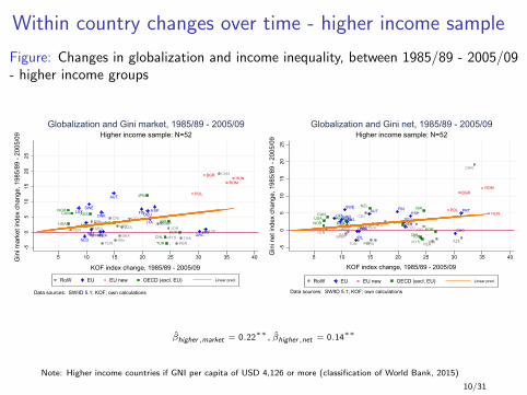
Within country changes over time - higher income sample

Figure: Changes in globalization and income inequality, between 1985/89 - 2005/09- higher income groups

DZAARGAZE

BWA BRA

CHN

COLCRIDOMECU

IRN

JOR

MYSPAN

PER

PRISGP

THA

TTO

TUN

URYVEN

AUT

BEL

DNKFIN

FRA

DEU

GRCIRL

ITA

LUX

NLD

PRT

ESPSWE

GBR

BGRHUN

POL

ROM

AUSCAN

CHL

ISR

JPN

KOR

MEXNZL

NOR

TUR

USA

-50

510

1520

25

Gin

i mar

ket i

ndex

cha

nge,

198

5/89

- 20

05/0

9

5 10 15 20 25 30 35 40


RoW EU EU new OECD (excl. EU) Linear pred.

Data sources: SWIID 5.1; KOF; own calculations

Higher income sample: N=52Globalization and Gini market, 1985/89 - 2005/09

DZAARG

AZEBWA

BRA

CHN

COL

CRI

DOMECU

IRN

JOR

MYS

PAN

PER

PRISGP

THA

TTO

TUN

URYVEN

AUT

BEL

DNK

FIN

FRA

DEU

GRC

IRL

ITA

LUXNLD

PRTESP

SWE

GBR

BGR

HUNPOL

ROM

AUSCAN

CHL

ISR

JPN

KORMEX

NZL

NOR

TUR

USA

-50

510

1520

25

Gin

i net

inde

x ch

ange

, 198

5/89

- 20

05/0

9

5 10 15 20 25 30 35 40




Higher income sample: N=52Globalization and Gini net, 1985/89 - 2005/09

βhigher,market = 0.22∗∗, βhigher,net = 0.14∗∗

Note: Higher income countries if GNI per capita of USD 4,126 or more (classification of World Bank, 2015)

10/31

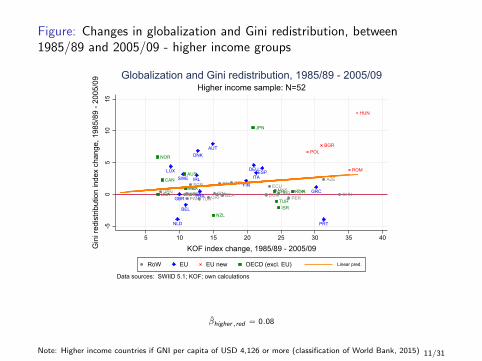
Figure: Changes in globalization and Gini redistribution, between1985/89 and 2005/09 - higher income groups

DZAARG

AZE

BWA

BRA

CHN

COL

CRI DOM

ECUIRN JORMYS

PAN PER

PRISGP

THATTO

TUNURYVEN

AUT

BEL

DNK

FIN

FRA

DEU

GRC

IRL ITALUX

NLD PRT

ESPSWE

GBR

BGR

HUN

POL

ROMAUS

CAN

CHL

ISR

JPN

KORMEX

NZL

NOR

TURUSA

-50

510

15

Gin

i red

istri

butio

n in

dex

chan

ge, 1

985/

89 -

2005

/09

5 10 15 20 25 30 35 40




Higher income sample: N=52Globalization and Gini redistribution, 1985/89 - 2005/09

βhigher,red = 0.08

Note: Higher income countries if GNI per capita of USD 4,126 or more (classification of World Bank, 2015) 11/31

3. OLS - fixed effects

12/31

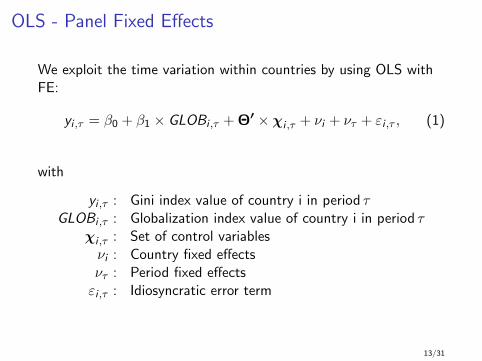
OLS - Panel Fixed Effects

We exploit the time variation within countries by using OLS withFE:

yi ,τ = β0 + β1 × GLOBi ,τ + Θ′ × χi ,τ + νi + ντ + εi ,τ , (1)

with

yi ,τ : Gini index value of country i in period τGLOBi ,τ : Globalization index value of country i in period τ

χi ,τ : Set of control variablesνi : Country fixed effectsντ : Period fixed effectsεi ,τ : Idiosyncratic error term

13/31

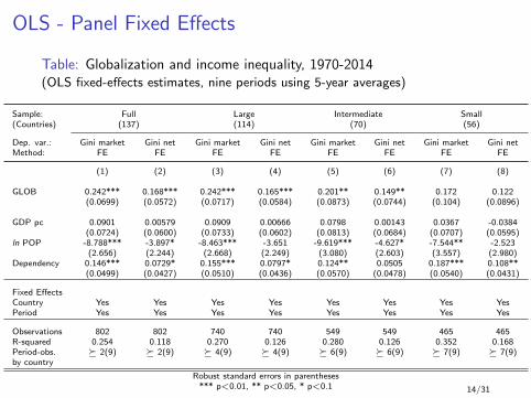
OLS - Panel Fixed Effects

Table: Globalization and income inequality, 1970-2014(OLS fixed-effects estimates, nine periods using 5-year averages)

Sample: Full Large Intermediate Small(Countries) (137) (114) (70) (56)

Dep. var.: Gini market Gini net Gini market Gini net Gini market Gini net Gini market Gini netMethod: FE FE FE FE FE FE FE FE

(1) (2) (3) (4) (5) (6) (7) (8)

GLOB 0.242*** 0.168*** 0.242*** 0.165*** 0.201** 0.149** 0.172 0.122(0.0699) (0.0572) (0.0717) (0.0584) (0.0873) (0.0744) (0.104) (0.0896)

GDP pc 0.0901 0.00579 0.0909 0.00666 0.0798 0.00143 0.0367 -0.0384(0.0724) (0.0600) (0.0733) (0.0602) (0.0813) (0.0684) (0.0707) (0.0595)

ln POP -8.788*** -3.897* -8.463*** -3.651 -9.619*** -4.627* -7.544** -2.523(2.656) (2.244) (2.668) (2.249) (3.080) (2.603) (3.557) (2.980)

Dependency 0.146*** 0.0729* 0.155*** 0.0797* 0.124** 0.0505 0.187*** 0.108**(0.0499) (0.0427) (0.0510) (0.0436) (0.0570) (0.0478) (0.0540) (0.0431)

Fixed EffectsCountry Yes Yes Yes Yes Yes Yes Yes YesPeriod Yes Yes Yes Yes Yes Yes Yes Yes

Observations 802 802 740 740 549 549 465 465R-squared 0.254 0.118 0.270 0.126 0.280 0.126 0.352 0.168Period-obs. 2(9) 2(9) 4(9) 4(9) 6(9) 6(9) 7(9) 7(9)by country

Robust standard errors in parentheses*** p<0.01, ** p<0.05, * p<0.1 14/31

4. IV strategy and 2SLS

15/31

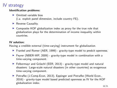
IV strategyIdentification problems:

I Omitted variable bias(i.a. exploit panel dimension, include country FE).

I Reverse Causality.

I Composite KOF globalization index as proxy for the true role thatglobalization plays for the determination of income inequality withincountries.

IV solution:Having a credible external (time-varying) instrument for globalization.

I Frankel and Romer (AER, 1999) - gravity-type model to predcit openness.

I Feyrer (NBER-WP, 2009) - gravity-type model in combination with atime-varying component.

I Felbermayr and Groschl (EER, 2013) - gravity-type model and naturaldisasters: Large-scale natural disasters (in other countries) as exogenoustime-varying component.

I Potrafke (J.Comp.Econ, 2013), Eppinger and Potrafke (World Econ.,2016) - gravity-type model based predicted openness as IV for the KOFglobalization index.

16/31

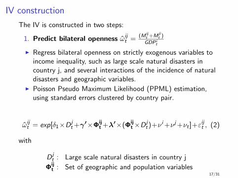
IV construction

The IV is constructed in two steps:

1. Predict bilateral openness ωijt = (M ij

t +M jit )

GDP it

I Regress bilateral openness on strictly exogenous variables toincome inequality, such as large scale natural disasters incountry j, and several interactions of the incidence of naturaldisasters and geographic variables.

I Poisson Pseudo Maximum Likelihood (PPML) estimation,using standard errors clustered by country pair.

ωijt = exp[δ1×D j

t +γ′×Φijt +λ′×(Φij

t ×D jt)+ν i +ν j +νt ]+ε

ijt , (2)

with

D jt : Large scale natural disasters in country j

Φijt : Set of geographic and population variables

17/31

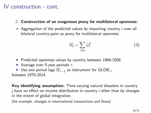
IV construction - cont.

2. Construction of an exogenous proxy for multilateral openness:

I Aggregation of the predicted values by importing country i over allbilateral country-pairs as proxy for multilateral openness:

Ωit =

∑i 6=j

ωijt (3)

I Predicted openness values by country between 1966-2008.I Average over 5-year periods τ .I Use one period lags Ωi

τ−1 as instrument for GLOBi,τ

between 1970-2014.

Key identifying assumption: Time-varying natural disasters in countryj have no effect on income distribution in country i other than by changesin the extent of global integration.

(for example, changes in international transactions and flows)

18/31

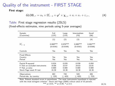
Quality of the instrument - FIRST STAGEFirst stage:

GLOBi,τ = α1 × Ωiτ−1 +ϕ′ × χi,τ + νi + ντ + εi,τ , (4)

Table: First stage regression results (2SLS)(fixed-effects estimates, nine periods using 5-year averages)


(1) (2) (3) (4)

Ωiτ−1 0.069*** 0.076*** 0.080*** 0.082***

(0.0155) (0.0159) (0.0162) (0.0168)

Controls Yes Yes Yes Yes

Fixed EffectsCountry Yes Yes Yes YesPeriod Yes Yes Yes Yes

Partial R-squared 0.024 0.029 0.039 0.050F-Test on excluded instruments 19.88 22.67 24.63 23.81F-Test, p-value 0.000 0.000 0.000 0.000Stock-Yogo weak IV test 16.38 16.38 16.38 16.38

Observations 802 740 549 465Period-obs. by country 2(9) 4(9) 6(9) 7(9)

Note: Robust standard errors in parentheses. The weak instruments hypothesis is rejectedwith the most stringent criterion - Stock and Yogo (2005) critical value of 10 percent.

*** p<0.01, ** p<0.05, * p<0.1 19/31

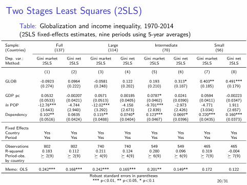
Two Stages Least Squares (2SLS)

Table: Globalization and income inequality, 1970-2014(2SLS fixed-effects estimates, nine periods using 5-year averages)


Dep. var.: Gini market Gini net Gini market Gini net Gini market Gini net Gini market Gini netMethod: 2SLS 2SLS 2SLS 2SLS 2SLS 2SLS 2SLS 2SLS

(1) (2) (3) (4) (5) (6) (7) (8)

GLOB -0.0923 0.0964 -0.0581 0.122 0.193 0.313* 0.403** 0.491***(0.274) (0.222) (0.248) (0.202) (0.210) (0.187) (0.185) (0.179)

GDP pc 0.0532 -0.00207 0.0571 0.00185 0.0787* 0.0241 0.0594 -0.00223(0.0533) (0.0421) (0.0513) (0.0405) (0.0462) (0.0390) (0.0411) (0.0347)

ln POP -12.76*** -4.744 -12.02*** -4.158 -9.701*** -2.973 -4.771 1.911(3.643) (2.940) (3.292) (2.673) (2.839) (2.426) (3.034) (2.657)

Dependency 0.102** 0.0635 0.115** 0.0740* 0.123*** 0.0697* 0.220*** 0.160***(0.0516) (0.0424) (0.0488) (0.0404) (0.0467) (0.0396) (0.0435) (0.0373)


Observations 802 802 740 740 549 549 465 465R-squared 0.183 0.112 0.211 0.124 0.280 0.096 0.319 -0.004Period-obs. 2(9) 2(9) 4(9) 4(9) 6(9) 6(9) 7(9) 7(9)by country

Memo: OLS 0.242*** 0.168*** 0.242*** 0.165*** 0.201** 0.149** 0.172 0.122


5. Results by development levels

21/31

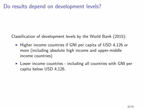
Do results depend on development levels?

Classification of development levels by the World Bank (2015):

I Higher income countries if GNI per capita of USD 4,126 ormore (including absolute high income and upper-middleincome countries)

I Lower income countries - including all countries with GNI percapita below USD 4,126.

22/31

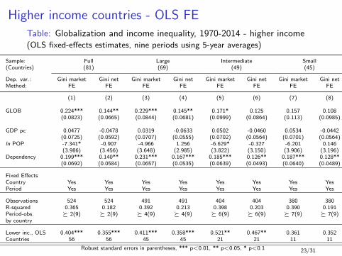
Higher income countries - OLS FE

Table: Globalization and income inequality, 1970-2014 - higher income(OLS fixed-effects estimates, nine periods using 5-year averages)



(1) (2) (3) (4) (5) (6) (7) (8)

GLOB 0.224*** 0.144** 0.229*** 0.145** 0.171* 0.125 0.157 0.108(0.0823) (0.0665) (0.0844) (0.0681) (0.0999) (0.0864) (0.113) (0.0985)

GDP pc 0.0477 -0.0478 0.0319 -0.0633 0.0502 -0.0460 0.0534 -0.0442(0.0725) (0.0592) (0.0707) (0.0555) (0.0702) (0.0564) (0.0701) (0.0564)

ln POP -7.341* -0.907 -4.966 1.256 -6.629* -0.327 -6.201 0.146(3.986) (3.456) (3.648) (2.985) (3.822) (3.150) (3.906) (3.196)

Dependency 0.199*** 0.140** 0.231*** 0.167*** 0.185*** 0.126** 0.187*** 0.128**(0.0692) (0.0584) (0.0657) (0.0535) (0.0639) (0.0493) (0.0640) (0.0489)



Lower inc., OLS 0.404*** 0.355*** 0.411*** 0.358*** 0.521** 0.467** 0.361 0.352Countries 56 56 45 45 21 21 11 11

Robust standard errors in parentheses, *** p<0.01, ** p<0.05, * p<0.1 23/31

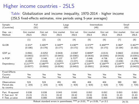
Higher income countries - 2SLS

Table: Globalization and income inequality, 1970-2014 - higher income(2SLS fixed-effects estimates, nine periods using 5-year averages)



(1) (2) (3) (4) (5) (6) (7) (8)

GLOB 0.321* 0.405** 0.349** 0.436** 0.373** 0.469*** 0.360* 0.462**(0.186) (0.178) (0.177) (0.172) (0.176) (0.173) (0.184) (0.182)

GDP pc 0.0561 -0.0252 0.0428 -0.0367 0.0695* -0.0131 0.0663 -0.0218(0.0453) (0.0377) (0.0443) (0.0365) (0.0416) (0.0345) (0.0418) (0.0341)

ln POP -5.832 3.148 -3.127 5.727* -3.646 4.738 -3.426 4.988(4.090) (3.618) (3.691) (3.227) (3.664) (3.196) (3.638) (3.176)

Dependency 0.217*** 0.186*** 0.252*** 0.219*** 0.219*** 0.184*** 0.219*** 0.183***(0.0577) (0.0503) (0.0526) (0.0453) (0.0501) (0.0426) (0.0497) (0.0422)


Observations 524 524 491 491 404 404 380 380Period-obs. 2(9) 2(9) 4(9) 4(9) 6(9) 6(9) 7(9) 7(9)by country

Part. R-squared 0.038 0.038 0.043 0.043 0.052 0.052 0.053 0.053F-Test excl. IV 23.15 23.15 24.42 24.42 23.91 23.91 21.43 21.43F-Test, p-value 0.000 0.000 0.000 0.000 0.000 0.000 0.000 0.000

Robust standard errors in parentheses; *** p<0.01, ** p<0.05, * p<0.1 24/31

6. The role of transition countries

25/31

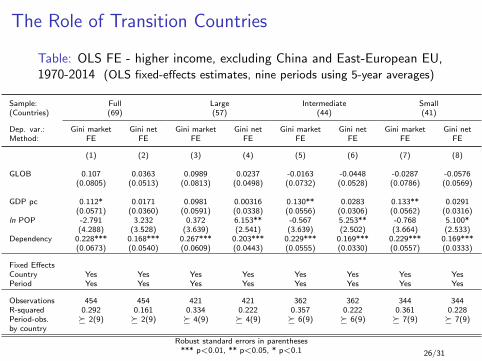
The Role of Transition Countries

Table: OLS FE - higher income, excluding China and East-European EU,1970-2014 (OLS fixed-effects estimates, nine periods using 5-year averages)



(1) (2) (3) (4) (5) (6) (7) (8)

GLOB 0.107 0.0363 0.0989 0.0237 -0.0163 -0.0448 -0.0287 -0.0576(0.0805) (0.0513) (0.0813) (0.0498) (0.0732) (0.0528) (0.0786) (0.0569)

GDP pc 0.112* 0.0171 0.0981 0.00316 0.130** 0.0283 0.133** 0.0291(0.0571) (0.0360) (0.0591) (0.0338) (0.0556) (0.0306) (0.0562) (0.0316)

ln POP -2.791 3.232 0.372 6.153** -0.567 5.253** -0.768 5.100*(4.288) (3.528) (3.639) (2.541) (3.639) (2.502) (3.664) (2.533)

Dependency 0.228*** 0.168*** 0.267*** 0.203*** 0.229*** 0.169*** 0.229*** 0.169***(0.0673) (0.0540) (0.0609) (0.0443) (0.0555) (0.0330) (0.0557) (0.0333)




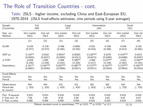
The Role of Transition Countries - cont.

Table: 2SLS - higher income, excluding China and East-European EU,1970-2014 (2SLS fixed-effects estimates, nine periods using 5-year averages)



(1) (2) (3) (4) (5) (6) (7) (8)

GLOB -0.429 -0.126 -0.396 -0.0901 -0.551 -0.190 -0.549 -0.181(0.377) (0.272) (0.346) (0.254) (0.418) (0.286) (0.413) (0.284)

GDP pc 0.110** 0.0162 0.0931* 0.00201 0.128*** 0.0278 0.143*** 0.0313(0.0505) (0.0327) (0.0492) (0.0311) (0.0473) (0.0295) (0.0496) (0.0297)

ln POP -6.828 2.005 -2.909 5.399** -3.606 4.427** -3.914 4.355**(4.226) (3.228) (3.222) (2.220) (3.317) (2.136) (3.382) (2.192)

Dependency 0.151** 0.145*** 0.202*** 0.188*** 0.172*** 0.153*** 0.175*** 0.156***(0.0697) (0.0530) (0.0560) (0.0417) (0.0517) (0.0343) (0.0503) (0.0332)


Observations 454 454 421 421 362 362 344 344Period-obs. 2(9) 2(9) 4(9) 4(9) 6(9) 6(9) 7(9) 7(9)by country

Part. R-squared 0.015 0.015 0.018 0.018 0.016 0.016 0.018 0.018F-Test excl. IV 7.66 7.66 8.56 8.56 6.82 6.82 6.67 6.67F-Test, p-value 0.006 0.006 0.004 0.004 0.010 0.010 0.010 0.010

Robust standard errors in parentheses; *** p<0.01, ** p<0.05, * p<0.1 27/31

7. Summary and outlook

28/31

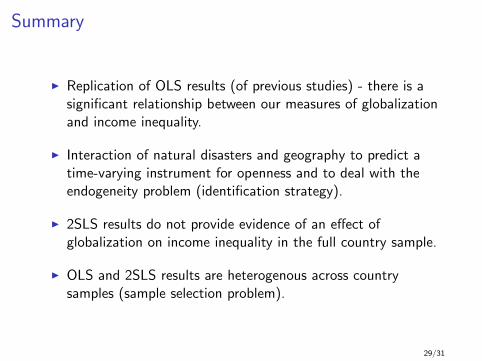
Summary

I Replication of OLS results (of previous studies) - there is asignificant relationship between our measures of globalizationand income inequality.

I Interaction of natural disasters and geography to predict atime-varying instrument for openness and to deal with theendogeneity problem (identification strategy).

I 2SLS results do not provide evidence of an effect ofglobalization on income inequality in the full country sample.

I OLS and 2SLS results are heterogenous across countrysamples (sample selection problem).

29/31

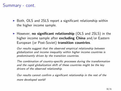
Summary - cont.

I Both, OLS and 2SLS report a significant relationship withinthe higher income sample.

I However, no significant relationship (OLS and 2SLS) in thehigher income sample after excluding China and/or EasternEuropean (or Post-Soviet) transition countries.

Our results suggest that the observed empirical relationship betweenglobalization and income inequality within higher income countries ispredominantly driven by the transition countries.

The combination of country-specific processes during the transformationand the rapid globalization shift of these countries might be the keydrivers of the observed relationship.

Our results cannot confirm a significant relationship in the rest of the

more developed world!

30/31

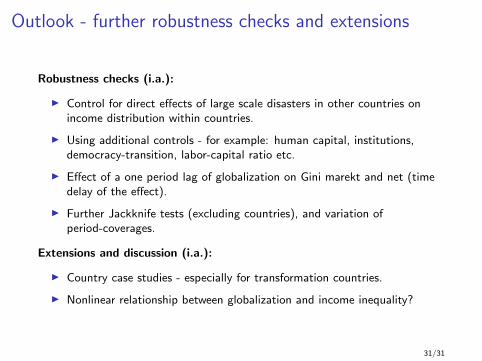
Outlook - further robustness checks and extensions

Robustness checks (i.a.):

I Control for direct effects of large scale disasters in other countries onincome distribution within countries.

I Using additional controls - for example: human capital, institutions,democracy-transition, labor-capital ratio etc.

I Effect of a one period lag of globalization on Gini marekt and net (timedelay of the effect).

I Further Jackknife tests (excluding countries), and variation ofperiod-coverages.

Extensions and discussion (i.a.):

I Country case studies - especially for transformation countries.

I Nonlinear relationship between globalization and income inequality?

31/31

APPENDIX

1/5

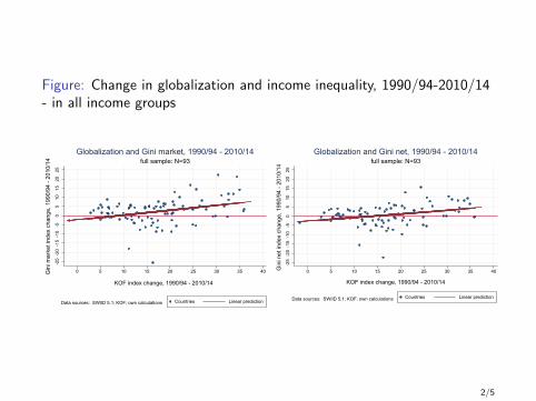
Figure: Change in globalization and income inequality, 1990/94-2010/14- in all income groups

-25

-20

-15

-10

-50

510

1520

25

Gin

i mar

ket i

ndex

cha

nge,

199

0/94

- 20

10/1

4

0 5 10 15 20 25 30 35 40



full sample: N=93Globalization and Gini market, 1990/94 - 2010/14

-25

-20

-15

-10

-50

510

1520

25

Gin

i net

inde

x ch

ange

, 199

0/94

- 20

10/1

40 5 10 15 20 25 30 35 40



full sample: N=93Globalization and Gini net, 1990/94 - 2010/14

2/5

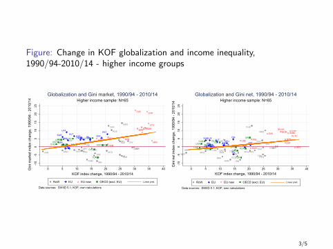
Figure: Change in KOF globalization and income inequality,1990/94-2010/14 - higher income groups

ARGBLR

BRA

CHN

COL

CRI

DOM

ECU

IRN

JOR

KAZ

MKD

MYS

NAM

PAN

PRY

PER

PRI

RUS

SGPZAF

THA

TUNURY

VEN

AUT

BEL

DNK FIN

FRA

DEUGRCIRLITA

LUX

NLD

PRT

ESPSWE

GBR

BGR

HRV

CYP

CZE

EST

HUN

LVA

LTU

POL

ROM

SVK

SVN

AUS

CAN

CHL

ISL

ISR

JPN

KORMEX NZL

NOR

CHE

TUR

USA

-10

-50

510

1520

25

Gin

i mar

ket i

ndex

cha

nge,

199

0/94

- 20

10/1

4

0 5 10 15 20 25 30 35 40




Higher income sample: N=65Globalization and Gini market, 1990/94 - 2010/14

ARG

BLR

BRA

CHN

COL

CRI

DOM

ECU

IRN

JOR

KAZ

MKD

MYS

NAM

PAN

PRY

PER

PRI

RUS

SGPZAF

THA

TUN URYVEN

AUTBELDNK

FIN

FRA

DEU

GRC

IRL

ITA

LUX

NLDPRTESP

SWE

GBR

BGR

HRV

CYP

CZEEST

HUN

LVA

LTUPOL

ROMSVK

SVN

AUSCAN

CHL

ISLISR

JPN KORMEX

NZL

NORCHE

TUR

USA

-10

-50

510

1520

25

Gin

i net

inde

x ch

ange

, 199

0/94

- 20

10/1

40 5 10 15 20 25 30 35 40




Higher income sample: N=65Globalization and Gini net, 1990/94 - 2010/14

3/5

ReferencesAcemoglu, D. (1998). Why do new technologies complement skills? Directed technical change and wage inequality.Quaterly Journal of Economics, 113(4), pp. 1055-1090.

Acemoglu, D. (2002). Technical Change, Inequality, and the Labor Market. Journal of Economic Literature, 40(1),pp. 7-72.

Bergh, A., and Nilsson, T. (2010). Do liberalization and globalization increase income inequality? EuropeanJournal of Political Economy, 26, pp. 488-505.

Dabla-Norris, E., Kochhar, K., Suphaphiphat, N., Ricka, F., and Tsounta, E. (2015). Causes and Consequences ofIncome Inequality: A Global Perspective. IMF Staff Discussion Note, No. 15/13.

Doerrenberg, P., and Peichl, A. (2014). The impact of redistributive policies on inequality in OECD countries.Applied Economics, 46(17), pp. 2006-2086.

Dorn, F. (2016). On data and trends in income inequality around the world. CESifo DICE Report, Journal ofInstitutional Comparisons, forthcoming.

Dreher, A., and Gaston, N. (2008). Has globalisation increased inequality? Review of International Economics, 16,pp. 516-536.

Dreher, A., Gaston, N., and Martens, P. (2008). Measuring globalization - Gauging its consequences. Berlin:Springer.

Eppinger, P., and Potrafke, N. (2015). Did Globalization Influence Credit Market Deregulation? World Economy,39(3), pp. 444-473.

Feenstra, R., and Hanson, G. (1997). Foreign direct investment and relative wages, evidence from Mexico‘smaquiladoras. Journal of International Economics, 42, pp. 371-393.

Felbermayr, G., and Groschl, J. (2013). Natural Disasters and the Effect of Trade on Income: A New Panel IVApproach. European Economic Review, 58, pp. 18-30.

Feyrer, J. (2009). Trade and Income - Exploiting Time Series in Geography. National Bureau of EconomicResearch Working Paper, No. 14910.

4/5

References cont.Frankel, J., and Romer, D. (1999). Does trade cause growth? American Economic Review, 89(3), pp. 379-399.

Gozgor, G., and Ranjan, P. (2015). Globalization, Inequality, and Redistribution: Theory and Evidence. CESifoWorking Paper No. 5522.

Meltzer, A., and Richard, S. (1981). A rational theory of the size of government. Journal of Political Economy,89(5), pp. 914-927.

Ohlin, B. (1933). Interregional and International Trade. Cambridge: Harvard University Press.

Potrafke, N. (2013). Globalization and Labor Market Institutions: International Empirical Evidence. Journal ofComparative Economics, 41(3), pp. 829-842.

Potrafke, N. (2015). The evidence on globalization. World Economy, 38(3), pp. 509-552.

Rodrik, D. (1998). Why do more open economies have bigger governments? Journal of Political Economy, 106(5),pp. 997-1032.

Roine, J., Vlachos, J., and Waldenstrom, D. (2009). The Long-Run Determinants of Inequality: What Can WeLearn from Top Income Data? Journal of Public Economics, 93(7-8), S. 974-988.

Savvides, A. (1998). Trade policy and income inequality, new evidence. Economics Letters, 61, pp. 365-372.

Schinke, C. (2014). Government Ideology, Globalization, and Top Income Shares in OECD Countries. ifo WorkingPaper, 181.

Sinn, H.-W. (2003). The new systems competition. Oxford: Blackwell.

Solt, F. (2016), The Standardized World Income Inequality Database. Social Science Quarterly 97.

Stolper, W., and Samuelson, P. (1941). Protection and Real Wages. Review of Economic Studies, 9, pp. 58-73.

WDI (2015). World Development Indicators. Washington D.C.: The World Bank.

Wood, A. (1995). How trade hurt unskilled workers. Journal of Economic Perspectives, 9, pp. 57-80.5/5

Documents

Globalization and income inequality - revisitedec.europa.eu/economy_finance/events/2016/20161128-arc2016/... · Globalization and income inequality - revisited - ... MNG MWI MYS NAM