1  

The Geography of Crime in Rochester- Patterns over Time (2005-2011)

Note: Animated version of maps are posted separately

on the web page at the working papers section of http://www.rit.edu/cla/cpsi/

Working Paper

August 2012-10

Arindam Ghosh Center for Public Safety Initiatives Rochester Institute of Technology

Axg7612@rit.edu

Michael Lagenbacher Center for Public Safety Initiatives Rochester Institute of Technology

Mike.lagenbacher@gmail.com

Janelle Duda Center for Public Safety Initiatives

jmdgcj@rit.edu

John Klofas Center for Public Safety Initiatives

jmkgcj@rit.edu

2  

Introduction This paper provides maps of all FBI part 1 crimes which were reported in Rochester, New York from 2005 through 2011. The goal of the paper is to examine the patterns of reported crime over a time and space within the City. The offense definitions used here are from the official measure of crime known as the Federal Bureau of Investigation’s (FBI) Uniform Crime Reports (UCR). The FBI’s UCR Program is a nationwide, cooperative statistical effort of law enforcement agencies across the country (nearly 18,000 of them) voluntarily reporting data on crimes brought to their attention. In this case, the data was obtained from the Rochester Police department, which is collected by the New York State Division of Criminal Justice Services (NYSDCJS) and reported to the FBI. The data spanned a time period of over 7 years, from 2005-2011. This paper contains the crime density maps for the Part I crimes occurring in Rochester over the same time period.

We will start with a warning to the reader. This paper contains a large number of maps and a smaller number of charts. For us, these are important as ways of displaying the data, but they have been important to our analytic processes as well. We have found them to be useful in guiding our own thoughts and discussions about the problem of crime in Rochester. We hope they are useful to others in both trying to understanding that problem and in addressing it.

Even with this hope, however, we recognize that this is a lengthy set of maps and other data displays. So we want to start with a few general statements from the data that we think will summarize key points that may not be entirely obvious, and that we hope will tempt you to struggle through the rest of the paper.

First, it is important to note the trends shown in the data. Reductions in crime are shown for five of the eight categories of Part 1 crimes including murder, rape, robbery, arson, motor vehicle theft and larceny. Levels for aggravated assault and generally flat while burglary levels show a slight upward trend. Taken together, these data show that over 127,000 part 1 crimes were reported in Rochester for the seven years from 2005 through 2011.

An important point to be made, however, is that much of the information we get from official crime statistics, particularly when overall crime level or rate is discussed, is dominated by facts about larceny, the crime of lowest seriousness and highest frequency. In Rochester larceny (theft) accounts for nearly 60% of all Part 1 offenses. Combining crime number, then, can lead to confusion. For example, due to the way official crime measures are aggregated, crime index totals count each shoplifting the same as each murder. If you are not careful, such things can mask or distort the reality of crime as it is experienced within the community. Also, bear in mind that these are reported crimes, and as we know, there are many crimes which go unreported, so this does not tell is the whole story – only part of it.

While serious violent crime is less frequent than the aggregated data may initially suggest, with the exception of rape, it is highly concentrated geographically and those concentrations persist over time. These are the most important facts about the distribution of serious crime.

And, there are important implications to them. First and foremost, it should be clear that, across this community, people have very different experiences with crime in general, with the risk of becoming a victim in particular, and also with the criminal justice system as it responds to crime. We may live very different lives as a result. Recognizing that, it should also be apparent that seeing beyond the chasm that crime can create, in order to better understand one another, is both a difficult and important task.

But there are also more specific implications of these crime patterns. They crystalize the community’s responsibility for addressing them. Their persistence demands action. That action can take many forms. It includes the work of individuals and organizations which seek to mitigate the pain implicit in these patterns, and to reduce or prevent violence. It also includes the focus and concentration of appropriate government resources, including the police. Their work is shaped by these patterns. The distribution of serious violence makes them a salient part of the lives of those most affected by crime. And, these facts make clear the great value to be found in strong relationships between the police and the community where crime is highest.

3  

The data reviewed here make clear the need for extensive analysis of the distribution of crime and the value of the analyses that currently take place through the Monroe Crime Analysis Center and the Rochester Police Department. The combined work supports ongoing consideration of these specific issues:

1. Mapping crime over extended periods of time can provide a useful view of the degree to which “hot spots” persist over time.

2. The maps of highest crime concentration areas highlight the importance of small or even micro-environments as possible targets of focused crime reduction strategies.

3. The distribution of violent crime supports the value of geographically focused strategies in efforts to simultaneously affect levels of robbery, aggravated assault and homicide.

4. These distributions also suggest the value of tightly targeted strategies intended to reduce illegal gun carrying. 5. With regard to property crime, the persistence of burglary concentrations also supports the potential value of

geographically targeted strategies. 6. The concentrations also support the importance of targeting efforts to address safety concerns and fear of crime,

and to promote positive relations between the police and the community in areas where crime concentrations persist.

7. Likewise, the crime patterns reinforce the importance of making community services available to residents living in neighborhoods with concentrations of crime.

8. Consistent with our earlier work, these patterns reinforce the view that it is important to consider the impact of jail and prison re-entry where crime concentrations persist over time.

Please note: The animated versions of all of the crime maps covering 2005-2011 are available on the CPSI working papers page below this paper. They provide a dynamic view of the stability and change over time.

How Crime is Counted in the FBI UCR Classifying and Scoring are two primary functions involved in the UCR program. Classifying involves determining the proper crime category for the reported offense. Scoring follows classifying and is a count of the number of offenses. For reporting purposes, criminal offenses are classified into two major groups: Part I offenses and Part II offenses. Part I crimes are collectively known as Index crimes, this name is used because the crimes are considered quite serious, tend to be reported more reliably than others, and are reported directly to the police.

For Part I crimes, UCR indexes the reported offenses in two categories- Violent crimes and Property Crimes. Part I offense classification included (in order of hierarchy):

Hierarchy Violent Crimes Hierarchy Property Crimes 1 Murder 5 Burglary 2 Forcible Rape 6 Larceny-theft 3 Robbery 7 Motor Vehicle Theft 4 Aggravated Assault 8 Arson

Hierarchy rules are followed when reporting multiple-offense situations. In such cases, the offenses that are highest on the hierarchy list are reported and scored and not the other offenses involved.

Please note that for this paper we did not incorporate the FBI hierarchy rule in our offense counts. Instead we mapped all times the noted offense was reported even when reported with more serious crimes. This allows the full display of the data but it also means that our counts are higher for some offenses than the official FBI counts.

The UCR definitions of the Part I crimes are listed on the respective maps in the following pages.

4  

Part II offenses include all other reportable crimes not included in Part I. Only arrest data is reported to FBI for these categories: simple assault, curfew offenses and loitering, embezzlement, forgery and counterfeiting, disorderly conduct, driving under the influence, drug offenses, fraud, gambling, liquor offenses, offenses against the family, prostitution, public drunkenness, runaways, sex offenses, stolen property, vandalism, vagrancy, and weapons offenses. Part II crimes have not been mapped or discussed in this paper. UCR limits the reporting to the 8 categories of Part I crimes as they are the crimes most likely to be reported and most likely to occur with sufficient frequency to provide an adequate basis for comparison. Thus, crimes which are not readily brought to the attention of the police don’t make it to the UCR database. Such crimes include kidnapping (as they occur infrequently) and behavioral categories such as bullying. It should also be noted that the UCR only reports crimes that citizens report and police record. This presents a problem, as a majority of crime goes unreported; the National Crime Victimization Survey (NCVS), discussed below, shows that, while on the decline, the percentage of violent crimes not reported to the police is about 42% (Marcus, Krebs, Langton & Smiley-McDonald, 2012).

Other Ways of Measuring Crime The UCR provides detailed information on crime reported to the police. The U.S. Department of Justice’s also provides a measure of criminal victimization. The National Crime Victimization Survey (NCVS) uses an annual survey of a representative sample of approximately 40,000 households comprising nearly 75,000 people. The household members are interviewed twice during the year. The survey provides estimates of victimization by rape, sexual assault, robbery, assault, theft, household burglary, and motor vehicle theft for the population as a whole as well as for segments of the population such as women, the elderly, members of various racial groups, city dwellers, or other groups. The methodology does not permit local crime estimates. The NCVS complements the UCR by providing otherwise unavailable information about victims, offenders, and crime (including crime not reported to the police).

Another methodology for measuring crime is Self-Report Surveys. The basic approach of the self-report method is to ask individuals if they have engaged in delinquent or criminal behavior, and if so, how often they have done so. The self- reports of delinquent and criminal behavior would be the nearest data source to the actual behavior, and thus be unaffected by the potential layers of bias introduced between the actual behavior and the data when relying on official sources such as the UCR.

Paper Overview The following pages present density maps for all Part I crimes for each of the seven years in the form of “small multiples” which permit comparison across the seven years of data (2005-2011). Discussion of the distributions follows each map set. Finally, a technical appendix describing the mapping process concludes the paper. We recommend that you read this paper in color; the maps use varying colors to show the distribution of crime and some of this important information can be lost if read in black and white and gray scale.

5  

THIS PAGE INTENTIONALLY LEFT BLANK

If printed on both sides of the paper, the maps and descriptions can be viewed side by side.

6  

7  

Violent Crimes in Rochester (2005-2011)

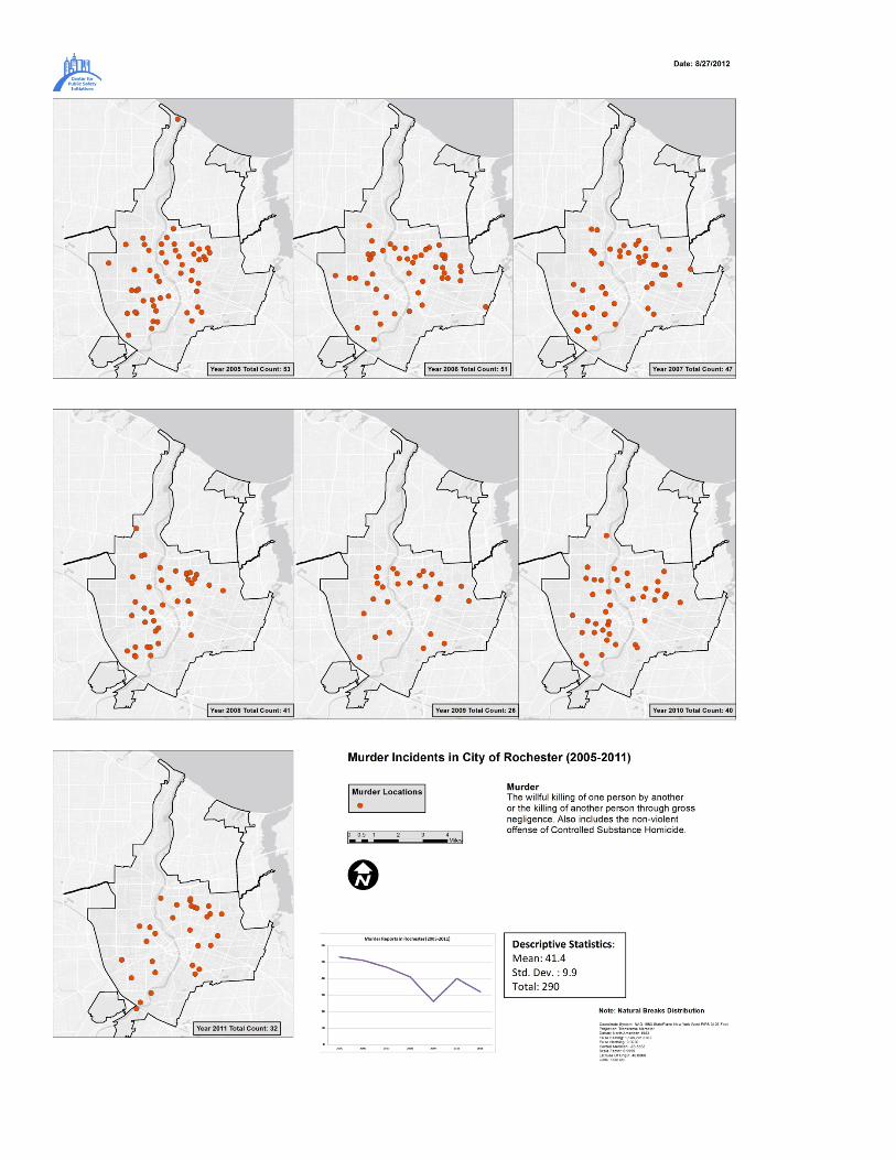
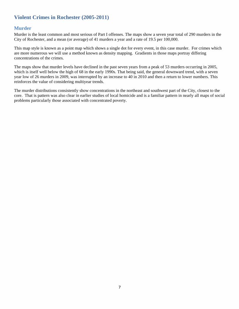
Murder Murder is the least common and most serious of Part I offenses. The maps show a seven year total of 290 murders in the City of Rochester, and a mean (or average) of 41 murders a year and a rate of 19.5 per 100,000.

This map style is known as a point map which shows a single dot for every event, in this case murder. For crimes which are more numerous we will use a method known as density mapping. Gradients in those maps portray differing concentrations of the crimes.

The maps show that murder levels have declined in the past seven years from a peak of 53 murders occurring in 2005, which is itself well below the high of 68 in the early 1990s. That being said, the general downward trend, with a seven year low of 26 murders in 2009, was interrupted by an increase to 40 in 2010 and then a return to lower numbers. This reinforces the value of considering multiyear trends.

The murder distributions consistently show concentrations in the northeast and southwest part of the City, closest to the core. That is pattern was also clear in earlier studies of local homicide and is a familiar pattern in nearly all maps of social problems particularly those associated with concentrated poverty.

8  

9  

Violent Crimes in Rochester (2005-2011)

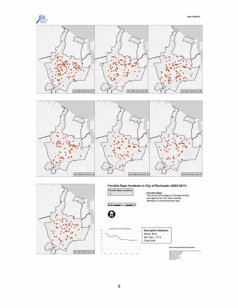
Forcible Rape*

Forcible Rape is the second most severe crime on the UCR hierarchy, but is also recognized as one of the least reported crimes. In fact, the NCVS suggests that approximately 65% of rape victims may not report the crime to the police (Marcus et al., 2012). Over the seven years of observation the city had an average (mean) of 92 rapes being reported each year, and a total of 644 rapes reported across the observation period. Like murder before it, the numbers of rapes observed in any given year were not numerous enough to warrant the use of a kernel density map. Instead, as with murder, each incident is represented by a point on the maps. Compared with murder, rape is more widely dispersed around the City even though the familiar shape of homicide patterns is visible in some years. This supports the view that the dynamics underlying these two offenses are quite different in many cases.

*Forcible rape is the term used to identify this crime in the FBI’s Uniform Crime Reports. In the period covered by this data it was defined as “the carnal knowledge of a female forcibly and against her will. Attempts or assaults to commit rape by force or threat of force are also included; however, statutory rape (without force) and other sex offenses are excluded.”

In June of this year the Justice Department announced a change in the definition of rape under the Uniform Crime Reports. Beginning in 2013 the UCR definition of rape will be “Penetration, no matter how slight, of the vagina or anus with any body part or object, or oral penetration by a sex organ of another person without consent of the victim.”

The revised definition includes any gender of victim or perpetrator, and includes instances in which the victim is incapable of giving consent because of temporary or permanent mental or physical incapacity, including due to the influence of drugs or alcohol or because of age. The ability of the victim to give consent must be determined in accordance with state statute. Physical resistance from the victim is not required to demonstrate lack of consent. The new definition does not change federal or state criminal codes or impact charging and prosecution on the local level.

With this change in definition, it is likely that in the coming years we will see an increase in the number of rapes reported. It is expected over the next several years, police departments will keep track of crimes under both definitions. This will provide some means of assessing whether changes in the number of rapes reported under the new definition reflect changes in offending behavior or changes in reporting due to the redefinition. Even with the change in the definition of rape, rape is expected to remain one of the most underreported crimes.

10  

11  

Violent Crimes in Rochester (2005-2011)

Robbery Robbery comprise the second largest category of Part I violent crimes in the dataset, with a total of 7,060 reports of occurrence over 7 years (2005-2011) and a mean of 1,008 occurrences each year.

The numbers of occurrences reported each year have been decreasing over the period of observation, with a peak year in 2006 with 1,377 robberies, and a low point in 2011 with 810 robberies.

Looking at the density maps over the years, it can be seen that there are some consistent hot spots (red areas) within the city limits, located mostly in the northeastern part of the city. The density of the crimes disperses over time as the total count decreases, with the highest areas of robbery density decreasing, while the general shape of the map remaining near constant. Some spots such as in the northern tip of the city, near Charlotte, show up on the map each year but indicated by a lower density, although robbery density peaks in the area in 2009. A possibility for their existence might be location of bars and pubs along that stretch of land and the persistent police presence in that area. Another observation is that a large portion of the hot spots are concentrated in the north-eastern part of the city, identified as a high crime area by the local community and the Rochester Police Department.

12  

13  

Violent Crimes in Rochester (2005-2011)

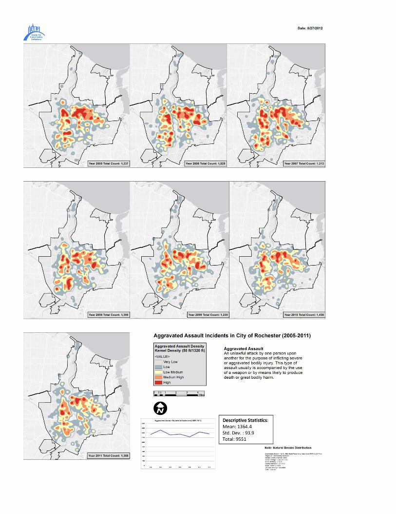
Aggravated Assault Aggravated Assaults comprise the largest category of Part I violent crimes in the dataset, with a total of 9,551 reports of occurrence over 7 years (2005-2011) and a mean of 1,364 occurrences each year.

The numbers of occurrences reported each year have been fairly constant, with occasional rises and falls. The prominent rises were seen in years 2006 and 2010, and the prominent fall was in year 2007. While the density patterns seem generally unaffected, total counts are affected by definitional changes which are reflected in the 2010 data. From, that year on, the crime of menacing, which involves threatening someone with a weapon, has been included in the count.

Looking at the density maps over the years, it is clear that a relatively similar pattern persists across the years and that there are some consistent hot spots (red areas) within the city limits, located mostly in the northern part of the city. The density of the crimes shift over time as the total count fluctuates. Some spots such as in the northern tip of the city, near Charlotte, show up on the map each year but indicated by a lower density. A factor contributing for their existence might be the location of bars and pubs along that stretch of land, seasonal differences and the persistent police presence in that area. Further observation reveals that with the increase in the crime count, the overarching shape of the density map takes the rough shape of a crescent, identified as a high crime area by the local community and the Rochester Police Department. The mapping of the crime lends support to this theory of the persistence of crime in some parts of the city.

14  

15  

Property Crimes in Rochester (2005-2011)

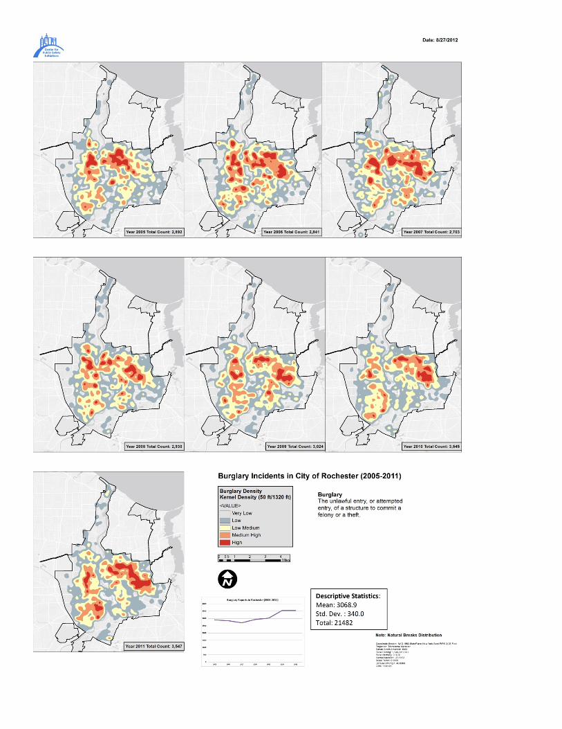
Burglary Burglaries comprise the second largest category of Part I property crimes in the dataset, with 21,482 reports of burglaries over the seven years (2005-2011), and an average (mean) of 3,068 burglaries a year.

Unlike most of the crimes covered in this paper, burglary levels are persistent and rising somewhat over time with the most prominent rise occurring in 2010, and 3,547 burglaries reported in 2011. Burglary is also somewhat unique in comparison to previously discussed crimes, as it is more widely distributed across the City. At the same time there is a clear and persistent concentration of these crimes in the northeastern portion of the city, with some additional smaller hot spots in the northwest and southwest part of the city.

16  

17  

Property Crimes in Rochester (2005-2011)

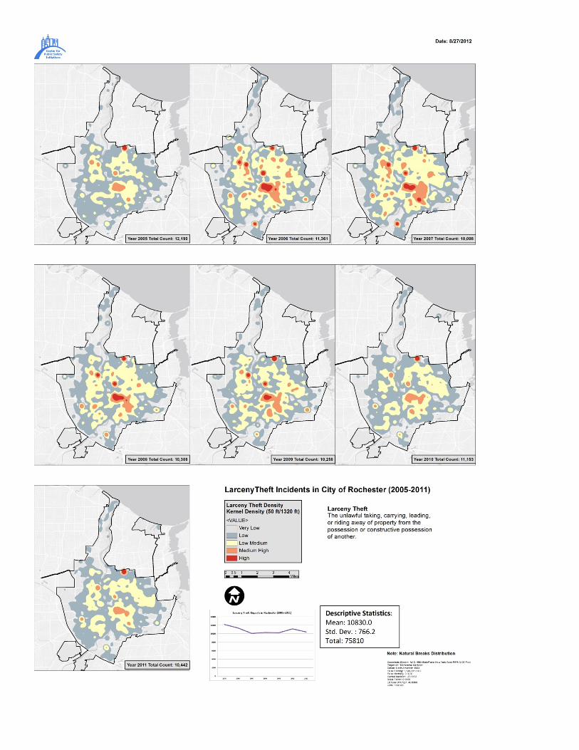
Larceny-Theft Larceny-thefts comprise the largest category of Part I property crimes in the dataset, with 75,810 reports of larcenies or thefts over the seven years (2005-2011), and an average (mean) of 10,830 larcenies a year.

The numbers of occurrences reported each year have been quite constant, with only small rises and falls. The most prominent rise was seen in 2010 , and prominent falls were seen in the years 2006, 2007, and 2011.

Looking at the density maps over the years, it can be seen that larcenies are spread throughout the city, and that there are several consistent hot spots (red areas) within the city limits. Most of these hotspots are located in commercial locations, such as the Walmart Supercenter in the northeast of the city (see our pervious paper on Larcenies from Walmart at http://www.rit.edu/cla/cpsi/WorkingPapers/2011/2011‐10.pdf), the shopping plaza on Clinton Avenue and the business district at the center of the city. Overall, the pattern of larceny density is relatively consistent, with very few changes in densities from year to year.

18  

19  

Property Crimes in Rochester (2005-2011)

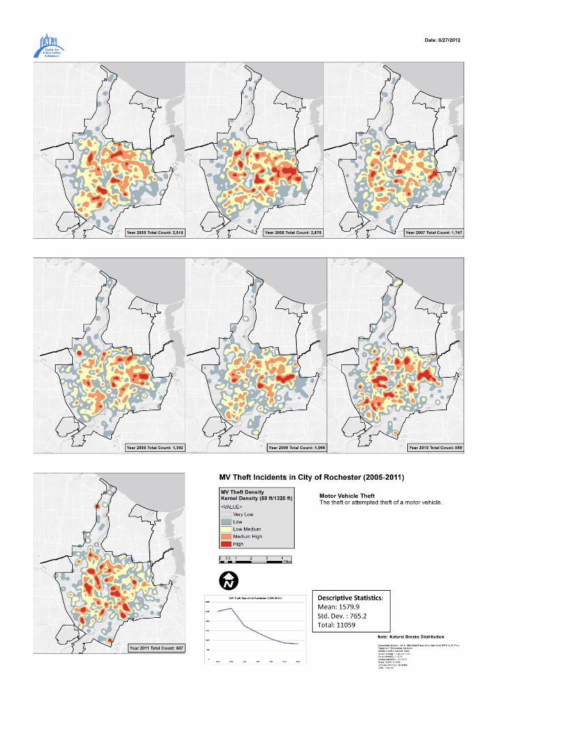
Motor Vehicle Theft Motor Vehicle Theft is the third largest category in Part I property crimes, with a total of 11,059 reported motor vehicle thefts across the seven years of observation (2005-2011), and an average (mean) of about 1,580 motor vehicle thefts a year.

The data show that he number of motor vehicle thefts has been steadily and dramatically decreasing during the past seven years. This mirrors national trends which show a 38% decline between 2006 and 2009. These reductions are due, in part, to police efforts and advances in technology available to both police and car owners. With the introduction of GPS as a feature in many new cars, tracking stolen cars is now much easier. In addition, the acquisition of new license plate reading technology by the police force in Rochester has made finding stolen cars and vehicles even easier.

As with most of the property crimes, motor vehicle theft seems to be spread throughout the city, with some areas, especially in the eastern part of the city, suffering from high motor vehicle theft density (red areas). The density maps also indicate little clear pattern of reported MV theft is seen over the period covered in the data. One interesting point of note is the emergence of two new hot spots, one in the North of the city and the other in the South of the city for the last year of study 2011, even as the total number of reported MV thefts are going down.

20  

21  

Property Crimes in Rochester (2005-2011)

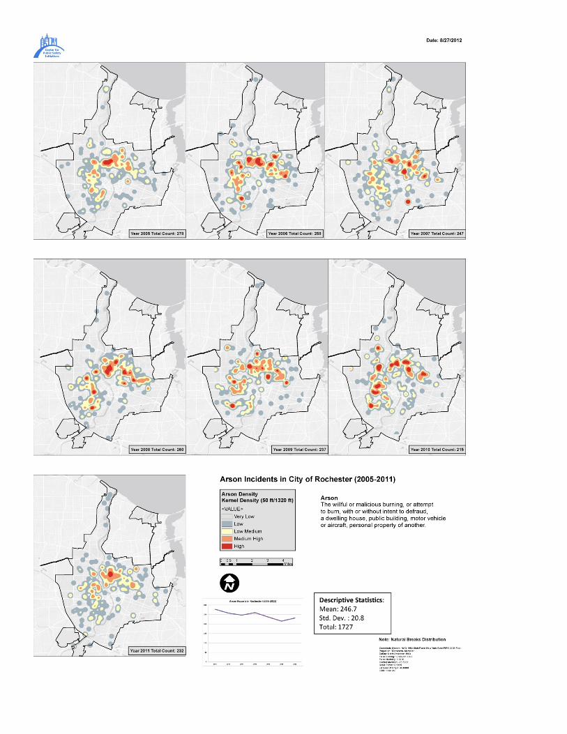
Arson Arson accounts for the smallest contributor to Part I property offenses, and is generally the lowest placed on the UCR hierarchy, despite the fact that arson can be an incredibly dangerous crime, not only causing damage to property, but also endangering lives of those near the arson. Over the course of seven years, there were 1,727 cases of arson reported by the police, and an average (mean) of 246 arsons a year.

While the number of arsons fluctuates mildly from year to year, they have remained relatively constant compared with other crimes. The pattern of arsons, while consistently forming a crescent shape (like those found in other crimes), vary from year to year in what areas see medium to high densities for the crime but remain concentrated in the City’s poorest neighborhoods where they are likely associated with the condition of property and the concentration of vacant or abandoned properties.

22  

Descriptive Statistics:Mean: 18231.9 Std. Dev. : 1483.8 Total: 127623 

23  

All Part 1 Crimes in Rochester  

These maps illustrate an important point. When considering the density of all Part I offenses (Violent and Property crimes) in Rochester as elsewhere, the resultant map resembles the density map of larceny. This is a result of the fact that over 50% of the total crimes in each year are classified as larceny (a mean of 10,830 larceny reports each year as compared to a mean of 18,230 Part I crimes each year.) In the map itself, one can see the hotspot in the northeast area of the city, where the Walmart is located, visible for each year of the data. This hotspot shows up consistently in the larceny maps as well.

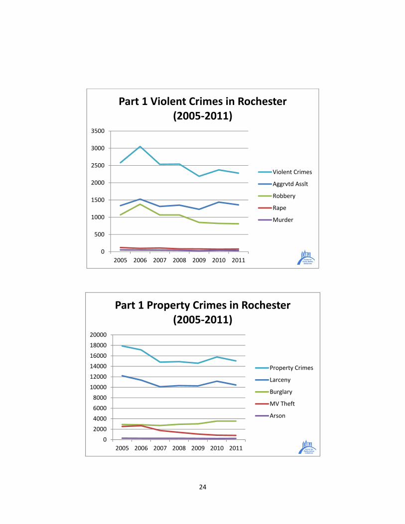
The overarching effect of larceny on the density maps of Part I crimes can also be verified by the graphs on the following page. The graph of the Part I property crimes closely follows the graph for the larceny. The effect of other crimes such as burglary (on the rise) or motor vehicle theft (on the decrease) seems to be nearly non-existent on the property crimes graph.

For Part I violent crimes, the total violent crime graph seems to be closely following the aggravated assault graph, as that category accounts for the largest share of violent crimes in the city. As such, a density map of only the violent crimes can be expected to resemble the density maps for aggravated assault.

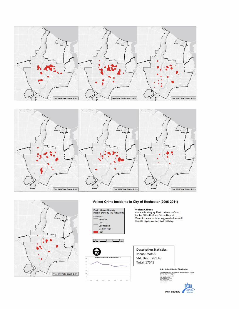
Maps of violent crime present a similar but less dramatic problem than the property crime map. The violent crime density map is most influenced by aggravated assault. This, of course, is attributable to the fact that aggravated assault reports make up more than 50% of all violent crimes in Rochester (a mean of 1,364 aggravated assaults per year compared to a mean of 2,506 violent crimes in the city). Thus, the aggravated assault reports influence the total violent crime count in the same way larceny reports influence the total Part I crime counts in Rochester. One thing of note is that the eastern part of the city suffers from a higher density of violent crimes than the rest of the city. There has been a net decline in the violent crime incidents in the city from 2006 to 2009, attributed to the decline in the number of aggravated assaults and robberies over the same time period. However, there is an increase in the number of violent offenses in 2010 primarily because of an increase in number of reported aggravated assaults associated with a change in definition, even though robbery offenses declined in the same year. This is another example of the influence of aggravated assaults on the total violent crime counts.

Much of the information we get from official crime statistics, when overall crime level or rate is discussed, includes all offenses and therefore is dominated by larceny, the crime of lowest seriousness and highest frequency. Aggravated assault has a similar effect on measures which combine all violent crime. These points are illustrated in the charts that follow. When the part 1 crimes are examined separately two things become clear. While serious violent crime is less frequent than the aggregated data may initially suggest, it is highly concentrated geographically and those concentrations have persisted over time. Our last set of maps provides the best illustration of this. These display only the areas with the highest levels of violent crime. Although there is some variation worth noting there is also considerable consistency across the time period.

The animations of all of the crime maps covering 2005-2011 are available on the CPSI working papers page below this paper. They provide a dynamic view of the stability and changes over time.

24  

0

500

1000

1500

2000

2500

3000

3500

2005 2006 2007 2008 2009 2010 2011

Part 1 Violent Crimes in Rochester (2005‐2011)

Violent Crimes

Aggrvtd Asslt

Robbery

Rape

Murder

0

2000

4000

6000

8000

10000

12000

14000

16000

18000

20000

2005 2006 2007 2008 2009 2010 2011

Part 1 Property Crimes in Rochester (2005‐2011)

Property Crimes

Larceny

Burglary

MV Theft

Arson

25  

Descriptive Statistics: Mean: 2506.0 Std. Dev. : 281.48 Total: 17545 

26  

Appendix: Mapping Crime In crime mapping, a ‘hot spot’ is a particular location or area that experiences a large amount of crime. Hot spots can be a place, a street, a neighborhood, a city or a region. Also, they are dynamic- they change over periods of time and the type of crime being analyzed. The changes can be in the form of shape, movement, appearance or disappearance. Hot spots analysis is the first step in any crime analysis effort as they are the result of processing large amounts of data and identifying places where there is a higher level of crime than other places. Hot spot analysis can be used to find areas for enforcement or further analysis of single event hot spots.

Hot spot analysis is usually categorized as five broad types(Paynich & Hill, 2010). The type of hot spot analysis used in this paper in Kernel Density analysis, also known as a type of grid cell mapping. This process involves the conversion of a large amount of point data into a continuously varying grid surface (called a raster) made up of small equally sized cells, whose size is specified by the analyst. Kernel Density calculates the density of point features around each output raster cell. In basic grid cell mapping, the analyst selects the cell size and specifies a search radius. The software counts the number of incidents within the radius and divides the number by the size of the search radius. Each cell then gets a score based on number of crimes near the cell divided by the area around the cell. In Kernel density, greater weight is assigned to incidents that occur close to the center of the search radius and lesser weight to those further out. The geospatial software utilized for this study is ArcGIS® Spatial Analyst, an optional extension to the ArcGIS Desktop product developed by ESRI.

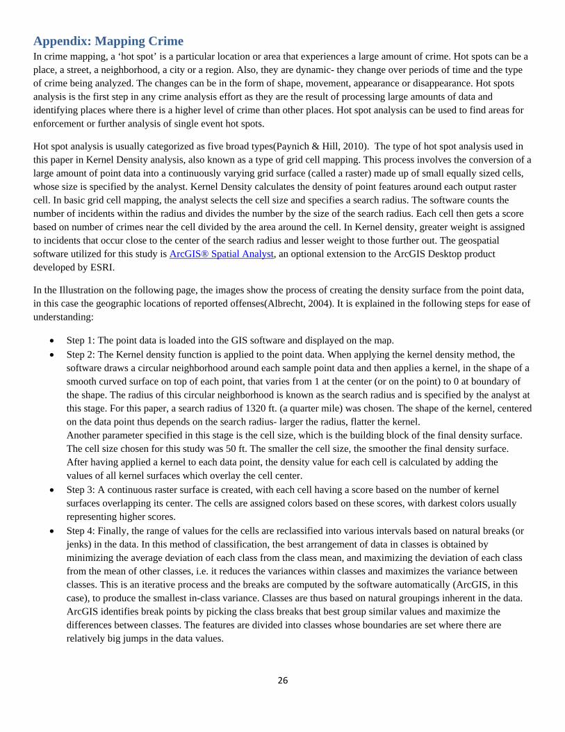
In the Illustration on the following page, the images show the process of creating the density surface from the point data, in this case the geographic locations of reported offenses(Albrecht, 2004). It is explained in the following steps for ease of understanding:

Step 1: The point data is loaded into the GIS software and displayed on the map.

Step 2: The Kernel density function is applied to the point data. When applying the kernel density method, the software draws a circular neighborhood around each sample point data and then applies a kernel, in the shape of a smooth curved surface on top of each point, that varies from 1 at the center (or on the point) to 0 at boundary of the shape. The radius of this circular neighborhood is known as the search radius and is specified by the analyst at this stage. For this paper, a search radius of 1320 ft. (a quarter mile) was chosen. The shape of the kernel, centered on the data point thus depends on the search radius- larger the radius, flatter the kernel.

Another parameter specified in this stage is the cell size, which is the building block of the final density surface. The cell size chosen for this study was 50 ft. The smaller the cell size, the smoother the final density surface. After having applied a kernel to each data point, the density value for each cell is calculated by adding the values of all kernel surfaces which overlay the cell center.

Step 3: A continuous raster surface is created, with each cell having a score based on the number of kernel surfaces overlapping its center. The cells are assigned colors based on these scores, with darkest colors usually representing higher scores.

Step 4: Finally, the range of values for the cells are reclassified into various intervals based on natural breaks (or jenks) in the data. In this method of classification, the best arrangement of data in classes is obtained by minimizing the average deviation of each class from the class mean, and maximizing the deviation of each class from the mean of other classes, i.e. it reduces the variances within classes and maximizes the variance between classes. This is an iterative process and the breaks are computed by the software automatically (ArcGIS, in this case), to produce the smallest in-class variance. Classes are thus based on natural groupings inherent in the data. ArcGIS identifies break points by picking the class breaks that best group similar values and maximize the differences between classes. The features are divided into classes whose boundaries are set where there are relatively big jumps in the data values.

27  

28  

References

Albrecht, J. (2004). Kernel Density Calculations. GTECH 361 Lecture 11  Retrieved Aug, 2012, from http://www.geography.hunter.cuny.edu/~jochen/GTECH361/lectures/lecture11/concepts/Kernel%20density%20calculations.htm 

Paynich, R., & Hill, B. (2010). Hot Spot Analysis Fundamentals of Crime Mapping. Sudbury, MA: Jones and Bartlett.