Combining police perceptions with police records of serious

crime areas

Robert Haining and Jane Law

Department of Geography

University of Cambridge

Outline1. Purpose of the study2. High Intensity Crime Areas (HIA)3. Constructing HIA:

1. Senior Police Officer perceptions2. Empirically defined from police records3. Comparing the two maps

4. Data Modelling:1. Model specification2. Results: modelling each map independently3. Results: combining the two maps

5. Discussion

1. Purpose of the Study

• Map the location of serious crime areas (HIA) in Sheffield using two valid but different data sources: senior police officers knowledge and database records;

• Go beyond descriptive mapping; “getting behind” the two maps using statistical models, in order to try to better understand the two spatial distributions;

• Examine ways of combining different types of knowledge.

2. High Intensity Crime Areas (HIA)

• Definition– HIA = areas of English cities that experience

high levels of violent (drug related) crime often perpetrated by people resident in the area special policing problems including witness intimidation. (Home Office, 1997)

– More than just “hot spots” (i.e. it is type rather than level of offending that is important).

“HIA appear to represent a particularly extreme manifestation of the co-existence in an area of serious crime, the victims of those crimes and the particularly dangerous individuals and groups responsible for committing those crimes” (Craglia et al 2001, p.1925)

• Conceptual roots– Social disorganization theory:

• Breakdown of internal social networks…• Population turnover…• Socio-economic or ethnic heterogeneity… ….leading to anti-social and eventually

criminal behaviour (Shaw and McKay, 1942)

• Powerlessness of some communities to influence decisions made externally and that ultimately have damaging consequences for them. (Bursik and Grasmick, 1993)

=> in UK context some areas become local authority “dumping grounds” for problem families. (Bottoms and Wiles, 2002)

- what may start out as “non-serious”

offences (vandalism etc) carried out by youth gangs and petty offenders evolve into something more substantial – often linked to the very profitable drugs market.

- motivated offenders go to greater lengths and violence becomes a feature of crime in such communities.

3. Constructing HIA (1998)

3.1 Senior Police Officer Perceptions (PHIA). STEP 1: South Yorkshire Police’s Performance

Review Department were given a list of factors:• serious gang culture;

• high propensity to violence;

• drugs problem;

• transient population;

• hostility towards police.

=> Identification of BCU-K

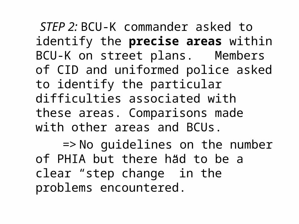
STEP 2: BCU-K commander asked to identify the precise areas within BCU-K on street plans. Members of CID and uniformed police asked to identify the particular difficulties associated with these areas. Comparisons made with other areas and BCUs.

=> No guidelines on the number of PHIA but there had to be a clear “step change” in the problems encountered.

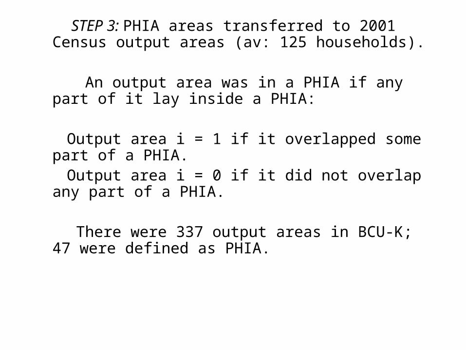
STEP 3: PHIA areas transferred to 2001 Census output areas (av: 125 households).

An output area was in a PHIA if any part of it lay inside a PHIA:

Output area i = 1 if it overlapped some part of a PHIA. Output area i = 0 if it did not overlap any part of a

PHIA.

There were 337 output areas in BCU-K; 47 were defined as PHIA.

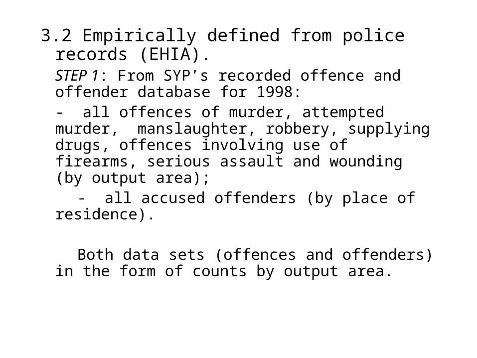
3.2 Empirically defined from police records (EHIA).STEP 1: From SYP’s recorded offence and offender database for 1998:- all offences of murder, attempted murder, manslaughter, robbery, supplying drugs, offences involving use of firearms, serious assault and wounding (by output area);

- all accused offenders (by place of residence).

Both data sets (offences and offenders) in the form of counts by output area.

Count statistics at the Output Area level

Average Standard deviation

Minimum Maximum

Offence counts 1.24 2.18 0 15

Offender counts 5.79 4.80 0 31

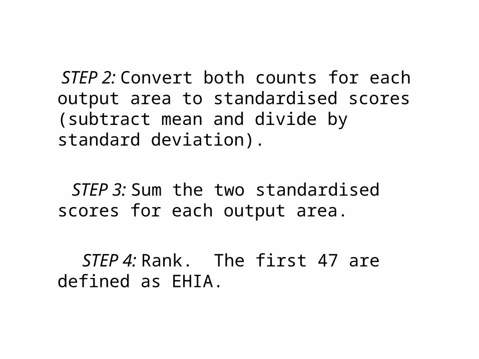
STEP 2: Convert both counts for each output area to standardised scores (subtract mean and divide by standard deviation).

STEP 3: Sum the two standardised scores for each output area.

STEP 4: Rank. The first 47 are defined as EHIA.

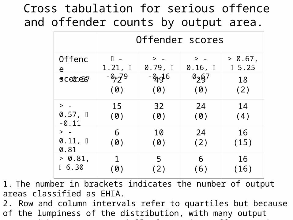
Cross tabulation for serious offence and offender counts by output area.  

 

Offender scores

Offence scores

-1.21, -0.79

> -0.79, -0.16

> -0.16, 0.67

> 0.67, 5.25

= -0.57 72(0)

49(0)

29(0)

18(2)

> -0.57, -0.11

15(0)

32(0)

24(0)

14(4)

> -0.11, 0.81

6(0)

10(0)

24(2)

16(15)

> 0.81, 6.30

1(0)

5(2)

6(6)

16(16)

1. The number in brackets indicates the number of output areas classified as EHIA.2. Row and column intervals refer to quartiles but because of the lumpiness of the distribution, with many output areas with 0 counts especially for serious offences, the row and column sums do not correspond to 25% of data values.

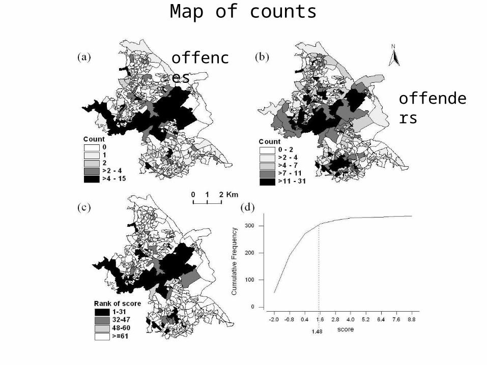
Map of counts

offences

offenders

3.3 Comparing the two maps

(a) Map overlay

(b) Spatially adjusted bivariate correlation (Clifford and Richardson, 1985)

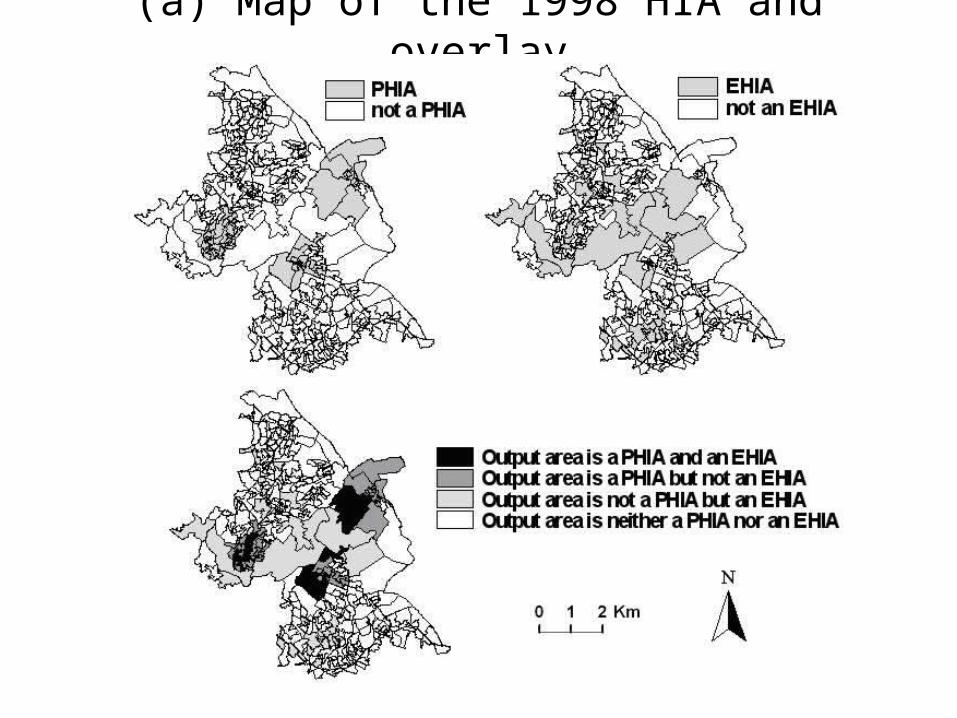
(a) Map of the 1998 HIA and overlay

(b) Spatially adjusted bivariate correlationNumber of bins

5 8 10 15 20 25 30

Break distance (metres)

2091 1307 1046 698 523 419 348

p-value .001 .015 .012 .020 .022 .035 .016

Effective sample size

940.4 486.4 525.7 449.4 436.1 368.4 475.8

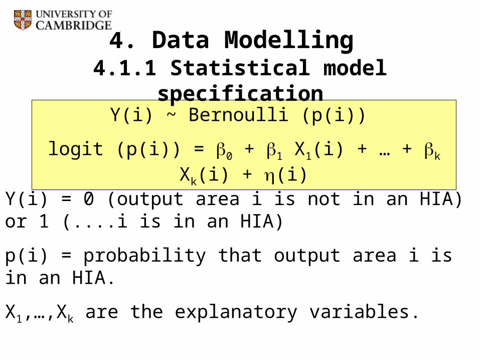
Y(i) ~ Bernoulli (p(i))

logit (p(i)) = 0 + 1 X1(i) + … + k Xk(i) + (i)

4. Data Modelling 4.1.1 Statistical model specification

Y(i) = 0 (output area i is not in an HIA) or 1 (....i is in an HIA)

p(i) = probability that output area i is in an HIA.

X1,…,Xk are the explanatory variables.

Model 1: An ordinary logistic regression model: (i) = 0 (Fitted in S-PLUS)

Model 2: A logistic regression model with spatial random effects: (i) = SCAR(i) which is a conditional spatial autoregressive model. (Fitted in WinBUGS)

This model allows us to recognize the spatial relationships between the output areas and to allow for the effects of spatially autocorrelated missing variables. The logit(p(i)) are now random variables.

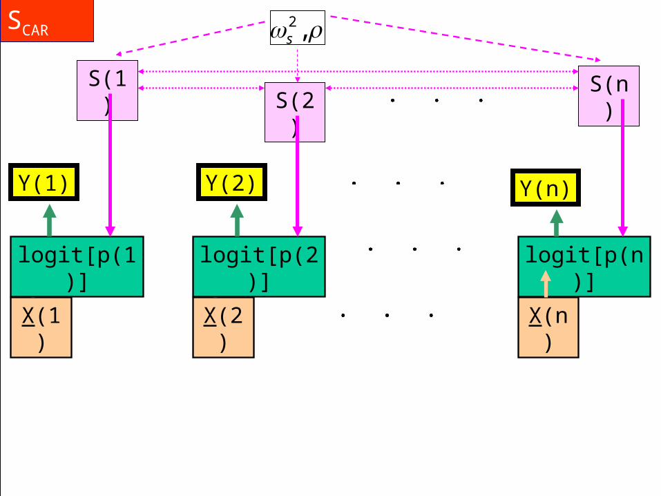
logit[p(n)]

Y(2)Y(1) Y(n)

X(n)X(1) X(2)

logit[p(1)] logit[p(2)]

,2s

S(1)S(2)

S(n)

SCAR

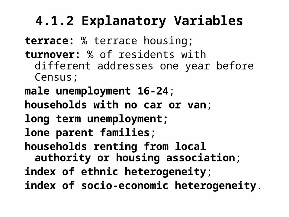
4.1.2 Explanatory Variables terrace: % terrace housing; turnover: % of residents with different addresses

one year before Census; male unemployment 16-24; households with no car or van;long term unemployment;lone parent families; households renting from local authority or

housing association; index of ethnic heterogeneity; index of socio-economic heterogeneity.

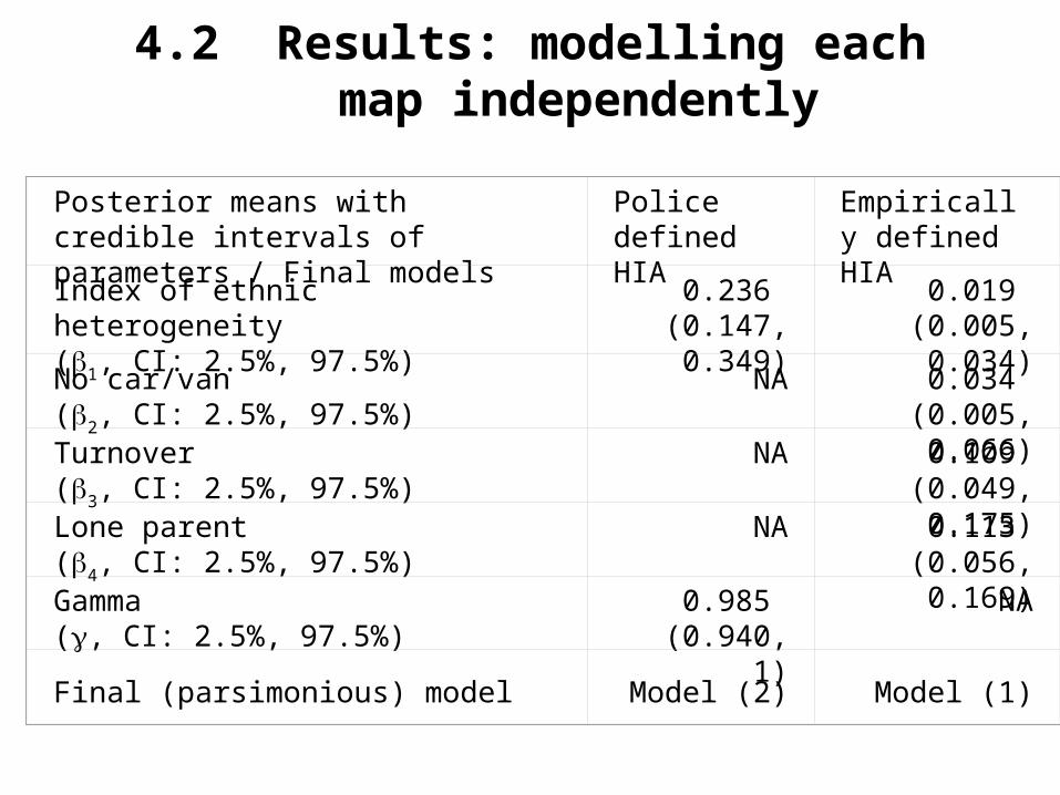
4.2 Results: modelling each map independently

Posterior means with credible intervals of parameters / Final models 

Police defined HIA

Empirically defined HIA

Index of ethnic heterogeneity(1, CI: 2.5%, 97.5%)

0.236 (0.147, 0.349)

0.019 (0.005, 0.034)

No car/van(2, CI: 2.5%, 97.5%)

NA 0.034 (0.005, 0.066)

Turnover(3, CI: 2.5%, 97.5%)

NA 0.109 (0.049, 0.175)

Lone parent(4, CI: 2.5%, 97.5%)

NA 0.113 (0.056, 0.169)

Gamma(, CI: 2.5%, 97.5%)

0.985 (0.940, 1)

NA

 

Final (parsimonious) model 

Model (2) 

Model (1)

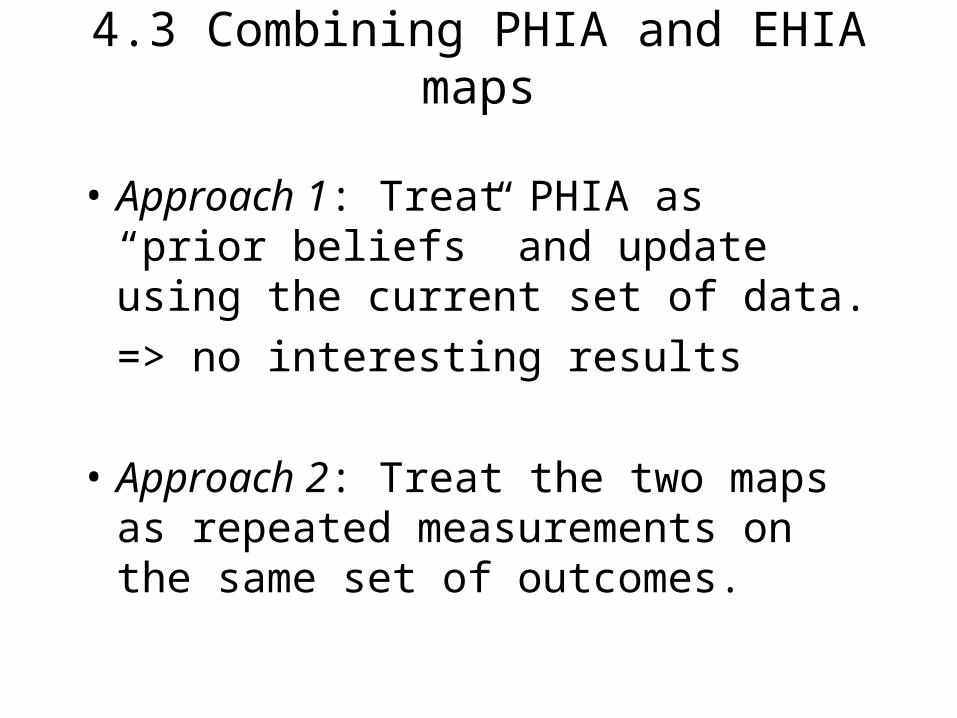
4.3 Combining PHIA and EHIA maps

• Approach 1: Treat PHIA as “prior beliefs” and update using the current set of data.

=> no interesting results

• Approach 2: Treat the two maps as repeated measurements on the same set of outcomes.

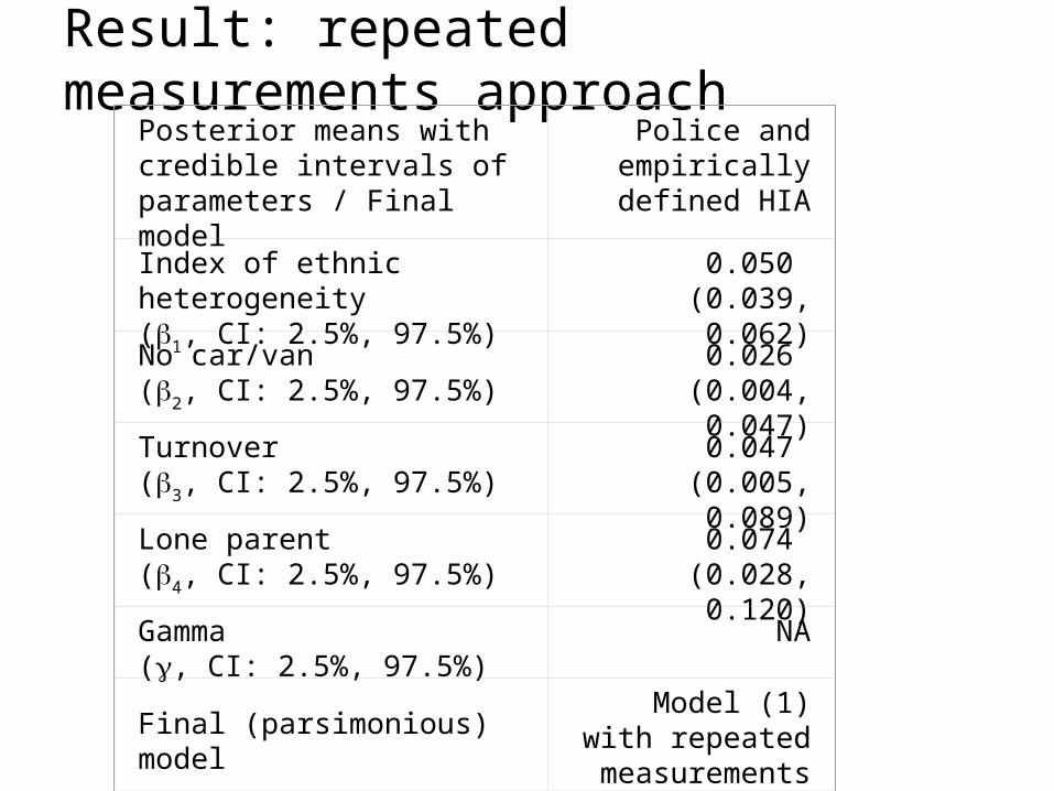
Result: repeated measurements approachPosterior means with credible intervals of parameters / Final model 

Police and empirically defined

HIA

Index of ethnic heterogeneity(1, CI: 2.5%, 97.5%)

0.050 (0.039, 0.062)

No car/van(2, CI: 2.5%, 97.5%)

0.026 (0.004, 0.047)

Turnover(3, CI: 2.5%, 97.5%)

0.047 (0.005, 0.089)

Lone parent(4, CI: 2.5%, 97.5%)

0.074 (0.028, 0.120)

Gamma(, CI: 2.5%, 97.5%)

NA

 

Final (parsimonious) modelModel (1) with

repeated measurements

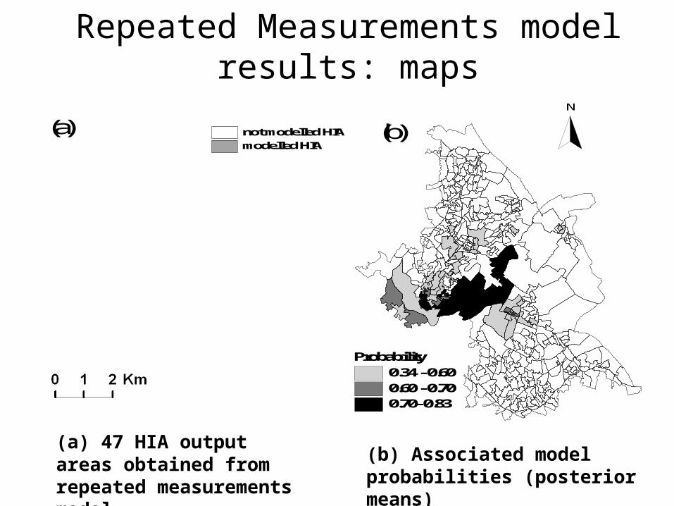
Repeated Measurements model results: maps

Probability0.34 - 0.600.60 - 0.700.70- 0.83

not modelled HIAmodelled HIA

N

(a) (b)

(a) 47 HIA output areas obtained from repeated measurements model

(b) Associated model probabilities (posterior means)

5. Discussion• The construction of good quality geocoded

offence/offender databases creates opportunities both for academic research and for the police and other services involved in local crime and disorder partnerships;

BUT• Tendency to use such databases for descriptive

mapping and;• To treat the database evidence as definitive when

compared to the police’s own knowledge (Ratcliffe and McCullagh 2001).

• Modelling offers an opportunity to understand the social, economic and demographic factors that underlie particular offence/offender geographies. (Academic importance; strategic benefit to the police?)

• Formally integrating both recorded crime data and the police’s own experience using GIS- or statistically-based methodologies may provide an effective way to exploit geocoded crime data:

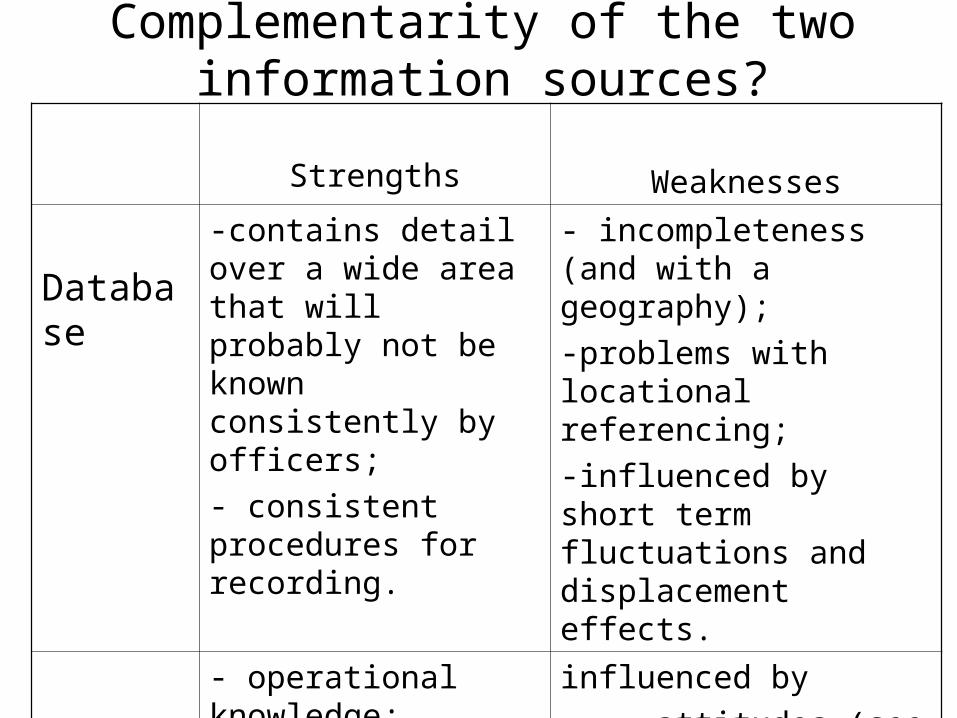
Complementarity of the two information sources?

Strengths Weaknesses

Database

-contains detail over a wide area that will probably not be known consistently by officers;

- consistent procedures for recording.

- incompleteness (and with a geography);

-problems with locational referencing;

-influenced by short term fluctuations and displacement effects.

Police officers

- operational knowledge;

- accumulated experience

influenced by

- attitudes (see Rengert and Palfrey 1997);

- what is/not remembered;

- particular experiences.

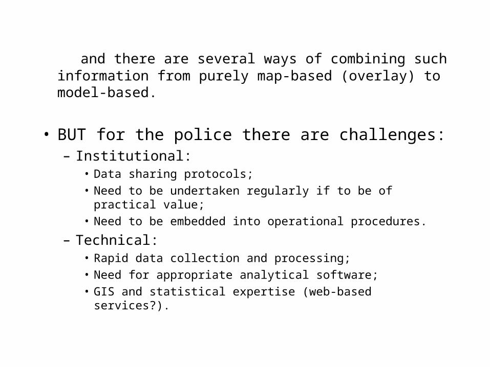
and there are several ways of combining such information from purely map-based (overlay) to model-based.

• BUT for the police there are challenges:– Institutional:

• Data sharing protocols;

• Need to be undertaken regularly if to be of practical value;

• Need to be embedded into operational procedures.

– Technical:• Rapid data collection and processing;

• Need for appropriate analytical software;

• GIS and statistical expertise (web-based services?).