Clemson UniversityTigerPrints

All Theses Theses

12-2015

The Gaussian Approximation to Multiple-AccessInterference in the Evaluation of the Performance ofa Communication System with ConvolutionalCoding and Viterbi DecodingSnigdhaswin KarClemson University

Follow this and additional works at: https://tigerprints.clemson.edu/all_theses

This Thesis is brought to you for free and open access by the Theses at TigerPrints. It has been accepted for inclusion in All Theses by an authorizedadministrator of TigerPrints. For more information, please contact kokeefe@clemson.edu.

Recommended CitationKar, Snigdhaswin, "The Gaussian Approximation to Multiple-Access Interference in the Evaluation of the Performance of aCommunication System with Convolutional Coding and Viterbi Decoding" (2015). All Theses. 2514.https://tigerprints.clemson.edu/all_theses/2514

The Gaussian Approximation to Multiple-AccessInterference in the Evaluation of the Performance of aCommunication System with Convolutional Coding and

Viterbi Decoding

A Thesis

Presented to

the Graduate School of

Clemson University

In Partial Fulfillment

of the Requirements for the Degree

Master of Science

Electrical Engineering

by

Snigdhaswin Kar

December 2015

Accepted by:

Dr. Daniel L. Noneaker, Committee Chair

Dr. Harlan B. Russell

Dr. Kuang-Ching Wang

Abstract

The standard Gaussian approximation is extended to the performance analysis

of direct-sequence code-division multiple-access (DS-CDMA) systems using binary con-

volutional coding, quaternary modulation with quaternary direct-sequence spreading and

Viterbi decoding. Using the standard Gaussian approximation, the random variables mod-

eling the multiple-access interference in the receiver statistics are replaced by an equivalent

additive Gaussian noise term with the same variance as the actual multiple-access interfer-

ence term. The Gaussian approximation is shown to result in an accurate approximation to

the probability of code-word error at the receiver. The accuracy is demonstrated by compar-

ing simulation results for the actual multiple-access system and a model using the standard

Gaussian approximation. Both are compared with two previously developed closed-form

bounds on the performance: the concave-first-event bound and the concave-integral bound.

ii

Acknowledgments

I would like to express my sincere gratitude to my advisor Dr. Daniel L. Noneaker for

his valuable guidance throughout my graduate studies, and his patience in the development

of this thesis. His support and in-depth knowledge of the subject have helped me immensely

in my research. I would also like to thank Dr. Harlan B. Russell and Dr. Kuang-Ching

Wang for serving as members of my committee and for sharing their knowledge and insight.

I also thank my colleagues in the Wireless Communication Systems and Networks group

for their help during my graduate studies.

I would like to thank my friends for their support and encouragement. I would also

like to extend a special thanks to my parents for their guidance and support.

iii

Table of Contents

Title Page . . . . . . . . . . . . . . . . . . . . . . . . . . . . . . . . . . . . . . . i

Abstract . . . . . . . . . . . . . . . . . . . . . . . . . . . . . . . . . . . . . . . . ii

Acknowledgments . . . . . . . . . . . . . . . . . . . . . . . . . . . . . . . . . . iii

List of Figures . . . . . . . . . . . . . . . . . . . . . . . . . . . . . . . . . . . . . v

1 Introduction . . . . . . . . . . . . . . . . . . . . . . . . . . . . . . . . . . . . 1

2 System Description . . . . . . . . . . . . . . . . . . . . . . . . . . . . . . . . 42.1 System Model . . . . . . . . . . . . . . . . . . . . . . . . . . . . . . . . . . . 42.2 Measures of the Quality of the Received Signal . . . . . . . . . . . . . . . . 102.3 Statistical Model of the Communication System . . . . . . . . . . . . . . . . 11

3 Characterization of the Receiver Statistics . . . . . . . . . . . . . . . . . . 12

4 Effect of the SGA on Pairwise Error-Event Probabilities . . . . . . . . . 22

5 Bounds on the Probability of Code-Word Error with Soft-Decision ViterbiDecoding . . . . . . . . . . . . . . . . . . . . . . . . . . . . . . . . . . . . . . 275.1 Concave-First-Event Bound . . . . . . . . . . . . . . . . . . . . . . . . . . . 285.2 Concave-Integral Bound . . . . . . . . . . . . . . . . . . . . . . . . . . . . . 28

6 Approximation of the Performance Using the SGA and Bounds . . . . . 296.1 Accuracy of the Approximations . . . . . . . . . . . . . . . . . . . . . . . . 30

7 Conclusion . . . . . . . . . . . . . . . . . . . . . . . . . . . . . . . . . . . . . 43

Bibliography . . . . . . . . . . . . . . . . . . . . . . . . . . . . . . . . . . . . . . 45

iv

List of Figures

2.1 System Model. . . . . . . . . . . . . . . . . . . . . . . . . . . . . . . . . . . 42.2 Transmitter for kth signal. . . . . . . . . . . . . . . . . . . . . . . . . . . . . 52.3 Channel. . . . . . . . . . . . . . . . . . . . . . . . . . . . . . . . . . . . . . . 72.4 Receiver. . . . . . . . . . . . . . . . . . . . . . . . . . . . . . . . . . . . . . . 9

4.1 Pairwise error-event probability as a function of Hamming distance. . . . . 26

6.1 Comparison of bounds for memory-order-two encoder (ρ=0). . . . . . . . . 346.2 Comparison of bounds for memory-order-two encoder (ρ=0.5). . . . . . . . 356.3 Comparison of bounds for memory-order-two encoder (ρ=1). . . . . . . . . 366.4 Comparison of bounds for memory-order-three encoder (ρ=0). . . . . . . . . 376.5 Comparison of bounds for memory-order-three encoder (ρ=0.5). . . . . . . . 386.6 Comparison of bounds for memory-order-three encoder (ρ=1). . . . . . . . . 396.7 Comparison of bounds for NASA-standard encoder (ρ=0). . . . . . . . . . . 406.8 Comparison of bounds for NASA-standard encoder (ρ=0.5). . . . . . . . . . 416.9 Comparison of bounds for NASA-standard encoder (ρ=1). . . . . . . . . . . 42

v

Chapter 1

Introduction

Direct-sequence spread-spectrum modulation is used in a number of wireless com-

munication networks that support multiple concurrent radio links within the same frequency

band in a given area. The most widely known of the networks are the cellular communica-

tion networks that employ direct-sequence spread-spectrum multiple-access communications

which is referred to as code-division multiple-access (or CDMA) communications in that

context [1]. A less well known application is in ad hoc packet-radio radio networks [2] which

are designed to provide robust digital communication capability in the absence of the fixed

infrastructure that is present in a cellular CDMA network.

There is much active research focused on developing improved protocols to support

greater data throughput and better quality of service in the highly dynamic environment

of an ad hoc packet radio network. The complexity of ad hoc networks is such that Monte

Carlo simulation of the networks is a key tool in the research, and high-fidelity simulation

requires extensive simulation time or computational resources. Much of the computational

burden comes from accurate simulation of the physical-layer communications (channel cod-

ing, modulation, demodulation, and decoding) in each link of the radio network. Any

technique that reduces the computational burden without sacrificing accuracy in the link

simulation is highly desirable.

That is the underlying motivation for the focus of this thesis. Specifically, we con-

1

sider a single communication link in a multiple-access interference environment and exam-

ine the accuracy of a key simplifying approximation to the link characteristics and simple

bounds on the link performance. The approximation is the standard Gaussian approxima-

tion (SGA), which replaces the terms in the receiver statistics of the link due to multiple-

access interference with an “equivalent” additive Gaussian noise term [3]. The closed-form

bounds were developed previously [4].

In this thesis, we consider a digital communication system in which the transmit-

ter employs binary convolutional coding, quaternary modulation with quaternary direct-

sequence spreading and the receiver employs coherent, soft-decision Viterbi decoding. The

received signal is corrupted by additive white Gaussian noise and possibly one or more

interfering signals from transmitters using the same transmission format as the desired sig-

nal. We consider the performance of the link as measured by the probability of error in the

detected code word provided as the output of the Viterbi decoder.

A closed-form expression is developed for the first and second moments of the

multiple-access interference terms in the receiver statistics of the system. They serve as

the basis for the SGA. The effect of the SGA to multiple-access interference is evaluated by

comparing the simulated performance of the system using actual interfering signals with sim-

ulation results using the SGA. The performance is also compared with closed-form bounds

on the performance which also make use of the SGA. Performance comparisons are provided

for several examples of a convolutional encoder and a range of multiple-access interference

channels.

In Chapter 2, we introduce the system model and develop the notation used in the

subsequent chapters. We discuss the transmitted signals and received signals and their

statistical models. The decision statistic is also discussed in this chapter and we define

various measures of the quality of the received signal. In Chapter 3, we develop closed-form

expressions for the first and second moments of the multiple-access interference terms in

the receiver statistics. The effect of the SGA on pairwise error-event probabilities in a

soft-decision Viterbi decoder is examined in Chapter 4. Two bounds on the probability

2

of code-word error are presented in Chapter 5. The accuracy of the approximations is

investigated in Chapter 6 for several examples of encoders and channels, and conclusions

are presented in Chapter 7.

3

Chapter 2

System Description

2.1 System Model

We consider a communication system with K transmitted signals using quaternary

modulation and quaternary, direct-sequence spreading [3], where each signal represents in-

formation from a different source. The system we consider is shown in Figure 2.1. Each

Figure 2.1: System Model.

transmitter uses a rate-j/n binary convolutional encoder of memory order m and a code-

symbol interleaver. The transmitted signal passes through a channel characterized by an

4

additive white Gaussian noise (AWGN) random process and it is corrupted by additive in-

terference from the other transmissions to give the received signal. The receiver converts the

received signal to a received word Z using a demodulator, a despreader and a deinterleaver.

The received word is decoded using soft-decision Viterbi decoding.

2.1.1 Transmitted Signal

The communication system considered in this thesis includes K transmitted signals,

sk(t), 0 ≤ k ≤ K − 1, and the transmitter for the kth signal is shown in Figure 2.2. The

information source at the transmitter generates the sequence of binary information words

d(i)k = (dk,ij(L−m), ..., dk,(i+1)j(L−m)−1), −∞ < i <∞. The ith information word is encoded

into the code word b(i)k = (bk,inL, ..., bk,(i+1)nL−1) using a rate-j/n binary convolutional

encoder of memory order m that is given by the generator polynomial G [5]. Each (L−m)j-

bit information word has mj tail bits appended prior to input into the encoder, which forces

the encoder to the all-zeros state at the end of the encoding [5] and results in L encoding

time steps per information word. Each code word is interleaved prior to transmission in an

rectangular array in which the code symbols are written into the array by rows and read out

of the array by columns. The ith interleaved code word is b(i)′

k = (b′k,inL, ..., b′k,(i+1)nL−1).

Figure 2.2: Transmitter for kth signal.

The kth transmitted signal, sk(t), is determined by the sequence of interleaved code

words {b(i)′

k }, −∞ < i < ∞. The binary code symbols from the kth transmitter form the

kth data signal,

b′k(t) =

∞∑i=−∞

(−1)b′k,ipT (t− iT ) (2.1)

5

where pT (t) is the unit pulse over [0,T ] and T is the bit duration. The kth data signal is

spread by inphase and quadrature spreading signals

aIk(t) =∞∑

l=−∞(−1)a

Ik,lψc(t− lTc) (2.2)

and

aQk (t) =

∞∑l=−∞

(−1)aQk,lψc(t− lTc) (2.3)

respectively, using N chips per code symbol, where the chip waveform ψc(t) is time-limited

to [0,Tc] and has total energy Tc. The inphase and quadrature binary spreading sequences

for the kth transmitted signal are thus{aIk,i

}, −∞ < i < ∞ and

{aQk,i

}, −∞ < i < ∞,

respectively. The data-modulated spreading inphase and quadrature signals are

cIk(t) = b′k(t)aIk(t) (2.4)

and

cQk (t) = b′k(t)aQk (t), (2.5)

respectively. They are modulated onto respective inphase and quadrature sinusoidal carri-

ers. The resulting kth transmitted signal is thus given by

sk(t) =√

2PkcIk(t)cos(2πfct+ θk) +

√2Pkc

Qk (t)sin(2πfct+ θk) (2.6)

where θk is the carrier phase angle, fc is the carrier frequency in Hertz, and Pk is the

transmitted power in each of the inphase and quadrature components of the transmitted

signal.

6

2.1.2 Channel

2.1.2.1 Channel Characterization

The transmitted signal s0(t) passes through an additive channel characterized by

the white Gaussian noise random process n(t), and interference from the other K − 1

transmissions. The channel is shown in Figure 2.3. Each transmitted signal undergoes a

Figure 2.3: Channel.

fixed attenuation, a delay, and a fixed Doppler shift between the transmitter and a receiver

that observes the received signal r(t). The channel results in a received signal that is the

sum of the attenuated, delayed transmitted signals and n(t). It is thus a multiple-access

additive white Gaussian noise (AWGN) channel, and

r(t) =K−1∑k=0

Aksk

((1 +

fkfc

)(t− τk)

)+ n(t) (2.7)

where the magnitude gain in the kth signal at the receiver is Ak, the fixed Doppler shift in

the kth signal at the receiver is fk, and the time delay of the kth signal at the receiver is

τk. The two-sided power spectral density of n(t) is N0/2.

7

2.1.2.2 Partial-Time Interference

In general, the channel we consider includes a set of interferers that transmit during

part of the transmission time of the desired signal and are idle during the rest of the desired

signal’s transmission. At a given time during the transmission of the desired signal, either

all K-1 interferers are active (in which case the received signal is given by equation (2.7)) or

none of the interferers are active (in which case the received signal is given by equation (2.7)

with K=1). The fraction of the transmission interval of the desired signal during which

the interferers are active is the interference activity of the system, which is denoted by ρ.

Thus, ρ=0 for a system without multiple-access interference, and ρ=1 for a system with

multiple-access interference present throughout the desired transmission. Simulation results

show that the performance of the system depends negligibly on the location of interference

activity within the received word for a given value of ρ if the system employs code-symbol

interleaving [4].

2.1.3 Receiver

The receiver is designed to detect the information originating at the transmitter

that sends s0(t). The summand for k = 0 in (2.7) is thus the desired component in the

received signal (or the desired signal, for short). For 1 ≤ k ≤ K − 1, the kth summand in

(2.7) is the kth interference component in the received signal (the kth interfering signal).

For example, if K =2, the received signal consists of the desired signal and one interfering

signal. Substituting (2.6) into (2.7),

r(t) =A0

√2P0c

I0(t)cos(2πfct) +

K−1∑k=1

Ak√

2PkcIk

((1 +

fkfc

)(t− τk)

)cos(2πfct+ Φk)+

A0

√2P0c

Q0 (t)sin(2πfct) +

K−1∑k=1

Ak√

2PkcQk

((1 +

fkfc

)(t− τk)

)sin(2πfct+ Φk)+

n(t)

(2.8)

8

where Φk = θk − 2π(fc + fk)τk + 2πfkt is the accumulated phase in the kth received

signal component at time t=0. The receiver is illustrated in Figure 2.4. We consider a

receiver that uses coherent demodulation and assume it achieves perfect symbol-timing

synchronization with the desired signal and a local carrier reference with perfect phase and

frequency synchronization with the desired signal. Without loss of generality, we assume

that θ0 = τ0 = f0 = 0 and we consider detection of information word d(0)0 .

Figure 2.4: Receiver.

The signal received during the interval [0, LT ) is converted to the received word Z ′

by a demodulator and a despreader for s0(t). The received word is decoded to the detected

information word d using soft-decision Viterbi decoding. In Chapter 4 and afterwards

in the thesis, we consider soft-decision Viterbi decoding using the correlator form of the

optimal (maximum-likelihood sequence detection) path metric [5]. The received word is

deinterleaved prior to decoding using a rectangular array in which the received symbols are

written into the array by columns and read out of the array by rows. The deinterleaved

received word is

Z = (Z0, ..., ZnL−1). (2.9)

9

2.1.4 Statistic for Each Binary Code Symbol

The output of the despreader is one statistic for each binary code symbol in the

code word b(0)0 . The symbol statistic Z ′i corresponding to code symbol b′0,i is given by

Z ′i =

∫ (i+1)T

iTr(τ)aI0(τ)cos(2πfcτ)dτ +

∫ (i+1)T

iTr(τ)aQ0 (τ)sin(2πfcτ)dτ

=S0,i +

K−1∑k=1

Ik,i + η0,i.

(2.10)

The term S0,i represents the contribution of the desired signal to the symbol statistic,

and the term Ik,i represents the contribution of multiple-access interference from the kth

interfering signal. The term η0,i represents the contribution of the thermal noise to the

decision statistic; it is a Gaussian random variable with mean zero and variance σ2η0,i = N0T2 .

The deinterleaved statistics {Z0, ..., ZnL−1} form the received word Z that is provided as

input to the Viterbi decoder.

2.2 Measures of the Quality of the Received Signal

The signal-to-noise ratio, the signal-to-interference ratio and the signal-to-interference-

plus-noise ratio of the desired signal at the receiver are used as the measures of the signal

quality. The signal-to-noise ratio, γSNR , in the ith channel-symbol position is defined as the

ratio of the (code-rate-normalized) desired-signal energy in Zi to the mean noise energy in

Zi:

γSNR =L(E[Zi]|b0,0)2

(L−m)Var(η0,i|b0,0)× 1

Rc. (2.11)

The signal-to-interference ratio, γSIR , in the ith channel-symbol position is defined as the

ratio of the normalized desired-signal energy in Zi to the mean interference energy in Zi:

γSIR =L(E[Zi]|b0,0)2

(L−m)Var(∑K−1

k=1 Ik,i|b0,0) × 1

Rc. (2.12)

10

The signal-to-interference-plus-noise ratio, γSINR , in the ith channel-symbol position is de-

fined as the ratio of the normalized desired-signal energy in Zi to the sum of the mean noise

energy and the mean interference energy in Zi:

γSINR =L(E[Zi]|b0,0)2

(L−m)Var((∑K−1

k=1 Ik,i + η0,i

)|b0,0

) × 1

Rc. (2.13)

2.3 Statistical Model of the Communication System

2.3.1 Transmitted Signal

The binary data symbols, {dk,i}, 0 ≤ k ≤ K − 1, 0 ≤ i ≤ j(L − m) − 1 and the

chip polarities,{aIk,i

}and

{aQk,i

}, 0 ≤ k ≤ K − 1, 0 ≤ i ≤ nL− 1 are modeled as mutually

independent Bernoulli random variables, with each random variable taking on the values 0

and 1, each with a probability of 1/2.

2.3.2 Received Signal

The time delays {τk} and the phase shifts {Φk}, 1 ≤ k ≤ K − 1, are mutually

independent random variables and they are mutually independent of the random variables

discussed in Section (2.3.1). Several circumstances are considered in subsequent chapters. In

one circumstance, the time delays and phase shifts are constant. In the other circumstances,

either each time delay is uniformly distributed over [0,T ], or each phase shift is uniformly

distributed over [0,2π], or both. In all the circumstances, the parameters {Pk}, {Ak}, and

{fk} are constant. In particular, we consider only fk = 0 for all k in the following chapters.

11

Chapter 3

Characterization of the Receiver

Statistics

In this chapter we characterize the code-symbol statistics at the receiver for the

system introduced in Chapter 2 and develop a joint Gaussian approximation to their joint

conditional distribution given the transmitted code word. The development is adapted

from the analysis given in [3] for a DS-CDMA system with offset QPSK spread-spectrum

data modulation in which the in-phase and quadrature spreading signals spread different

(offset) binary data signals. The circumstance we consider thus differs from the circumstance

considered in [3] in that the in-phase and quadrature spreading signals spread the same

binary data signal with no time offset between the inphase and quadrature signals. The

development in [3] addresses the effect of the Gaussian approximation on the probability of

error in a channel-symbol decision at the output of the receiver’s demodulator, whereas we

use the Gaussian approximation in an approximation of the probability of code-word error

at the output of the Viterbi decoder.

Without loss of generality, we consider the statistics Z ′0 and Z ′l and develop closed-

form expressions for their conditional first and second moments given the transmitted code

word for each of four special cases. In the first case, the time delays and phase shifts of

the interfering signals are constant. In the second case, each carrier’s phase shift at the

12

receiver for each interfering signal is uniformly distributed over [0,2π] but their time delays

are constant. In the third case, the time delay at the receiver for each interfering signal

is uniformly distributed over [0,T ] but its phase shift is constant. In the fourth case, each

time delay is uniformly distributed over [0,T ] and each phase shift is uniformly distributed

over [0,2π].

In all that follows, conditioning on b′0,0 is implicit. Following [3], from equation

(2.9),

E[S0,0] = (−1)b′0,0TA0

√2P0 (3.1)

and

Var(η0,0) =N0T

2. (3.2)

Furthermore,

Ik,0 =

√A2kPk2

(W Ik +WQ

k

)(3.3)

where

W Ik = U Ik cos(Φk) + V I

k sin(Φk) (3.4)

WQk = UQk cos(Φk)− V Q

k sin(Φk) (3.5)

U Ik =

(∫ T

0Ak√

2PkcIk (τ − τk) cos(2πfcτ + Φk)a

I0(τ)cos(2πfcτ)dτ

)/cos(Φk) (3.6)

UQk =

(∫ T

0Ak√

2PkcQk (τ − τk) sin(2πfcτ + Φk)a

Q0 (τ)sin(2πfcτ)dτ

)/cos(Φk) (3.7)

13

V Ik =

(∫ T

0Ak√

2PkcQk (τ − τk) sin(2πfcτ + Φk)a

I0(τ)cos(2πfcτ)dτ

)/sin(Φk) (3.8)

V Qk =

(∫ T

0Ak√

2PkcIk (τ − τk) cos(2πfcτ + Φk)a

Q0 (τ)sin(2πfcτ)dτ

)/sin(Φk). (3.9)

The random variables {U Ik , UQk , V

Ik , V

Qk }, 1 ≤ k ≤ K − 1, can be expressed in terms of

random variables involving discrete cross-correlation functions of the spreading sequences

and the chip-pulse continuous partial autocorrelation functions [3]. For example, the random

variable U Ik can be expressed as

U Ik =N−2∑i=0

HIk,i[Rψc(Sk) + aI0,ia

I0,i+1Rψc(Sk)]

+HIk,N−1Rψc(Sk) +HI

k,NRψc(Sk)

(3.10)

where

HIk,i =

(−1)b

′k,−1aIk,i−γka

I0,i, if 0 ≤ i ≤ γk − 1

(−1)b′k,0aIk,i−γka

I0,i, if γk ≤ i ≤ N − 1

(−1)b′k,−1aIk,−γk−1a

I0,0, if i = N

. (3.11)

The chip delay random variable Sk is given by Sk = τk−γkTc, with γk = bτk/Tcc. The chip

autocorrelation functions are given by

Rψc(s) =

∫ s

0ψc(t)ψc(t+ Tc − s)dt (3.12)

and

Rψc(s) =

∫ Tc

sψc(t)ψc(t− s)dt. (3.13)

14

Similarly, the random variable UQk can be expressed as

UQk =N−2∑i=0

HQk,i[Rψc(Sk) + aQ0,ia

Q0,i+1Rψc(Sk)]

+HQk,N−1Rψc(Sk) +HQ

k,NRψc(Sk)

(3.14)

where

HQk,i =

(−1)b

′k,−1aQk,i−γka

Q0,i, if 0 ≤ i ≤ γk − 1

(−1)b′k,−0aQk,i−γka

Q0,i, if γk ≤ i ≤ N − 1

(−1)b′k,−1aQk,−γk−1a

Q0,0, if i = N

. (3.15)

The random variable V Ik can be expressed as

V Ik =

N−2∑i=0

HIk,i[Rψc(Sk) + aI0,ia

I0,i+1Rψc(Sk)]

+ HIk,N−1Rψc(Sk) + HI

k,NRψc(Sk)

(3.16)

where

HIk,i =

(−1)b

′k,−1aQk,i−γka

I0,i, if 0 ≤ i ≤ γk − 1

(−1)b′k,−0aQk,i−γka

I0,i, if γk ≤ i ≤ N − 1

(−1)b′k,−1aQk,−γk−1a

I0,0, if i = N

. (3.17)

And the random variable V Qk can be expressed as

V Qk =

N−2∑i=0

HQk,i[Rψc(Sk) + aQ0,ia

Q0,i+1Rψc(Sk)]

+ HQk,N−1Rψc(Sk) + HQ

k,NRψc(Sk)

(3.18)

where

HQk,i =

(−1)b

′k,−1aIk,i−γka

Q0,i, if 0 ≤ i ≤ γk − 1

(−1)b′k,0aIk,i−γka

Q0,i, if γk ≤ i ≤ N − 1

(−1)b′k,−1aIk,−γk−1a

Q0,0, if i = N

. (3.19)

15

Under the independence conditions of Section 2.3, the random variables {HIk,i, H

Qk,i, H

Ik,i,

HQk,i}, 1 ≤ k ≤ K − 1, 0 ≤ i ≤ N , are mutually independent and identically distributed

(i.i.d.) equally likely Bernoulli random variables, as can be shown following an argument in

[6]. Define the correlation parameters

C ,N−2∑i=0

aQ0,iaQ0,i+1, 1 ≤ k ≤ K − 1, (3.20)

and

D ,N−2∑i=0

aI0,iaI0,i+1, 1 ≤ k ≤ K − 1. (3.21)

The random variables {U Ik , UQk , V

Ik , V

Qk }, 1 ≤ k ≤ K − 1, are conditionally mutually inde-

pendent given {C,D, {Φk, τk}, 1 ≤ k ≤ K−1}, again following an argument in [6]. Thus, the

conditional covariances of any two of the random variables is zero. Similarly, {W Ik ,W

Qk },

1 ≤ k ≤ K − 1, are conditionally mutually independent given {C,D, {Φk, τk}, 1 ≤ k ≤

K − 1}.

Now let us consider the first moment and variance of each of the random variables.

It is helpful to decompose the expression for each into useful auxiliary random variables.

As an example, we will consider the case of UQk . Define the disjoint sets of indices

A , {i, 0 ≤ i ≤ N − 2, such that aQ0,iaQ0,i+1 = 1} (3.22)

and

B , {i, 0 ≤ i ≤ N − 2, such that aQ0,iaQ0,i+1 = −1}. (3.23)

Then

UQk = λkRψc(Sk) + µkRψc(Sk) (3.24)

where the discrete random variables λk and µk are given by

λk = Xk + Yk +Hk,N−1 (3.25)

16

µk = Xk − Yk +Hk,N (3.26)

and the discrete variables Xk and Yk are defined by

Xk ,∑iεA

Hk,i (3.27)

and

Yk ,∑iεB

Hk,i. (3.28)

The random variables {λk, µk,Φk, τk}, 1 ≤ k ≤ K − 1, are conditionally mutually indepen-

dent given C and {Φk, τk}, 1 ≤ k ≤ K − 1, is independent of C.

It follows that

E[λk] = E[µk] = E[λkµk] = 0 (3.29)

and, using equation (3.24) and the independence conditions of Section 2.3, we have

E[UQk ] = E[λkRψc(Sk) + µkRψc(Sk)]

= E[Rψc(Sk)]E[λk] + E[Rψc(Sk)]E[µk] = 0.

(3.30)

In a similar manner,

E[V Qk ] = E[U Ik ] = E[V I

k ] = 0. (3.31)

17

Therefore,

E[Ik,0] = E

√A2kPk2

(U Ik cos(Φk) + V I

k sin(Φk) + UQk cos(Φk)− V Qk sin(Φk)

)=

√A2kPk2

(E[U Ik ]E[cos(Φk)] + E[V I

k ]E[sin(Φk)]

+E[UQk ]E[cos(Φk)]− E[V Qk ]E[sin(Φk)]

)= 0

(3.32)

from equations (3.30) and (3.31) and the independence conditions of Section 2.3.

Now we will proceed to find the expression for the variance of the multiple-access

interference term in equation (2.10). From the independence conditions of Section 2.3,

Var

(K−1∑k=1

Ik,0

)=

K−1∑k=1

Var (Ik,0) . (3.33)

And from the same independence conditions and equations (3.30) and (3.31),

Var (Ik,0) =1

2Var

[√A2kPk(W

Ik +WQ

k )

]=

1

2A2kPk

(E[(U Ik )2]E[cos2(Φk)] + E[(V I

k )2]E[sin2(Φk)]

+ E[(UQk )2]E[cos2(Φk)] + E[(V Qk )2]E[sin2(Φk)]

).

(3.34)

Furthermore,

E[(UQk )2] =E[(λkRψc(Sk) + µkRψc(Sk))2]

=E[λ2k]E[(Rψc(Sk))2] + E[µ2k]E[(Rψc(Sk))

2]

(3.35)

from equation (3.24) and the independence conditions of Section 2.3. Similar expressions

result for E[(U Ik )2], E[(V Ik )2], and E[(V Q

k )2]. Finally,

E[λ2k] = E[µ2k] = N. (3.36)

18

Thus,

Var (Ik,0) =1

2A2kPk

(2(NE[(Rψc(Sk))

2] +NE[(Rψc(Sk))2])E[cos2(Φk)]

+ 2(NE[(Rψc(Sk))2] +NE[(Rψc(Sk))

2])E[sin2(Φk)])

=A2kPkN

((E[(Rψc(Sk))

2] + E[(Rψc(Sk))2])(E[cos2(Φk)] + E[sin2(Φk)])

)=A2

kPkN(E[(Rψc(Sk))

2] + E[(Rψc(Sk))2]).

(3.37)

Note that equation (3.37) does not depend on the distribution function of Φk.

Case 1: Consider the case where {Φk, τk}, 1 ≤ k ≤ K−1 are constant. Let Sk = sk,

where sk is a constant.

We consider the rectangular chip pulse waveform, for which the partial autocorre-

lation functions are given by

Rψc(s) = s (3.38)

and

Rψc(s) = Tc − s. (3.39)

From equation (3.37),

Var (Ik,0) = A2kPkN(T 2

c + 2s2k − 2Tcsk). (3.40)

Case 2: The analysis of case 1 applies, so the variance of Ik,0 is given by equation

(3.40).

Case 3: Consider the case where τk is uniformly distributed over [0,T ] but Φk is

constant.

E[(Rψc(Sk))2] + E[(Rψc(Sk))

2] =2

Tc

∫ Tc

0R2ψc(s)ds = 2T 2

cMc (3.41)

where the term Mc , 1T 3c

∫ Tc0 R2

ψc(s)ds represents a chip mean-squared correlation parameter

that depends on the actual shape of the chip waveform ψc(t). We consider the rectangular

chip pulse waveform, for which the partial autocorrelation functions are given by equations

19

(3.38) and (3.39). Thus, Mc = 1/3, and

E[(Rψc(Sk))2] + E[(Rψc(Sk))

2] =2

3T 2c . (3.42)

From equation (3.37),

Var (Ik,0) =2

3A2kPkNT

2c . (3.43)

Case 4: The analysis of Case 3 applies, so the variance of Ik,0 is given by (3.43).

For cases 1 and 2, the signal-to-interference-plus-noise ratio in channel-symbol position zero

is given by

γSINR =2L(E[Z ′0])

2

(L−m)Var(∑K−1

k=1 Ik,0 + η0,0

)=

4LA20P0T

2

(L−m)(N0T2 +

∑K−1k=1 A

2kPkN(T 2

c + 2s2k − 2Tcsk))

=8LA2

0P0T2

(L−m)(N0T + 2∑K−1

k=1 A2kPkN(T 2

c + 2s2k − 2Tcsk)).

(3.44)

For cases 3 and 4, it is given by

γSINR =2L(E[Z ′0])

2

(L−m)Var(∑K−1

k=1 Ik,0 + η0,0

)=

8LA20P0T

(L−m)(N0 + 4∑K−1

k=1 A2kPkT/3N)

.

(3.45)

In a similar manner to the development above, it can be shown that the same results hold for

each Z ′l for which interference is present in the corresponding symbol interval and analogous

results hold with K=1 for each Z ′l for which interference is absent. Regardless, it is shown

in a similar manner that Z ′l1 and Z ′l2 are conditionally uncorrelated given b′0,l1 and b′0,l2 for

l1 6= l2.

In the subsequent chapters, we compare the performance of two systems. The

first system is the DS-CDMA system defined in Chapter 2, in which the desired signal is

20

subjected to both thermal noise and multiple-access interference at the receiver. In the

second system, the effect of the interference on the receiver statistics is approximated by

replacing each interference term Ik,l with a zero-mean Gaussian random variable Ik,l such

that the Var(Ik,l)=Var(Ik,l). The random variables {Ik,l, ηk,l}, 1 ≤ k ≤ K−1, 0 ≤ l ≤ nL−1

are independent. The second system thus approximates the first system using the SGA.

Two bounds on the probability of code-word error are considered in Chapter 5, and both

use the SGA (i.e., the model of the second system).

21

Chapter 4

Effect of the SGA on Pairwise

Error-Event Probabilities

In this chapter, we gain insight into the effect of the SGA on the probability of error

at the output of the soft-decision Viterbi decoder by considering the pairwise error-event

probability [4] in the decoder for error events of different Hamming weights. The interference

activity ρ=1. The receiver of the soft-decision Viterbi decoder provides maximum-likelihood

detection of the code word based on the continuous-valued channel outputs. We assume

without loss of generality that the all-zeros sequence is the actual transmitted sequence.

Let Z = (Z0, .., ZnL−1) denote the deinterleaved channel outputs under the condition

that the code sequence b(0)0 = (b0, .., bnL−1) = 0. Suppose bq+l−1q = (bq, ..., bq+l−1) is a length-

l subsequence of b(0)0 and b

q+l−1q = (bq, ..., bq+l−1) is the corresponding subsequence of code

sequence b for which the encoder states agree at times q and q + l in the generation of the

two sequences. Suppose d is the Hamming distance between the two code subsequences and

that they differ in code-symbol positions i0, ..., id−1. That is bij = 1, 0 ≤ j ≤ d − 1, and

bij = 0 for all i, q ≤ i ≤ q + l − 1, such that i 6∈ {io, .., id−1}.

Among the two subsequences, the soft-decision Viterbi decoder will prefer the sub-

sequence with the larger correlator-form path metric [5]. The path metric for bq+l−1q is given

22

by

M =

q+l−1∑i=q

Zi(−1)bi =

q+l−1∑i=q

Zi, (4.1)

and the path metric for bq+l−1q is given by

M =

q+l−1∑i=q

Zi(−1)bi

=

q+l−1∑i=q s.t. bi=0

Zi −q+l−1∑

i=q s.t.bi=1

Zi.

(4.2)

The probability of the pairwise error-event {M > M} is thus given by

P (M > M) = P

− q+l−1∑i=q s.t. bi=1

Zi >

q+l−1∑i=q s.t. bi=1

Zi

= P

q+l−1∑i=q s.t. bi=1

Zi < 0

= P (X < 0)

(4.3)

where

X =d−1∑j=0

Zij . (4.4)

Suppose the SGA is used to approximate the effect of the multiple-access interference on

the receiver statistics of the system in Chapter 2 with soft-decision Viterbi decoding. Then

{Zi0 , ..., Zil−1} are independent, identically distributed Gaussian random variables with

E[Zij ] = TA0

√2P0 (4.5)

from equation (2.10) and

Var(Zij ) =N0T

2+

K−1∑k=1

A2kPkN

(E[(Rψc(Sk))

2] + E[(Rψc(Sk))2])

(4.6)

23

from equations (3.2) and (3.37). (The form of the latter equation can be simplified in any

of the four cases considered in the previous chapter.) Then

P (M > M) =Q

(dE[Zi0 ]√dVar(Zi0)

)

=Q

(√2dA2

0P0T 2

(N0T2 +

∑K−1k=1 A

2kPkN(E[(Rψc(Sk))

2] + E[(Rψc(Sk))2]))

)

=Q

(√2dEc

(N0 +∑K−1

k=1 2A2kPkN(E[(Rψc(Sk))

2] + E[(Rψc(Sk))2]))

) (4.7)

where Ec is the energy per channel symbol at the receiver. For example, if Φk = τk = 0 for

1 ≤ k ≤ K − 1 and all the signals are received with the same strength,

P (M > M) =Q

(√2dEc

(N0 + (K − 1)Ec/N)

). (4.8)

Thus in two limiting cases,

P (M > M) = Q

(√2dEcN0

)(4.9)

if no multiple-access interference is present in the received signal, and

P (M > M) = Q

(√2dN

K − 1

)(4.10)

if no thermal noise is present in the received signal.

The effect of the SGA on the accuracy of the pairwise error-event probability is

illustrated by considering the system of Chapter 2 using soft-decision Viterbi decoding with

a spreading factor of 31 chips per binary channel symbol (N = 31), a single interfering

signal (K = 2) that is chip synchronous and phase synchronous with the desired signal,

and interference activity ρ=1. The desired signal and the interfering signal arrive at the

receiver with the same power.

The pairwise error-event probability in the decoder is illustrated in Figure 4.1 for

24

several values of the Hamming distance of the error event. The solid lines in the figure

show pairwise error-event probabilities for the system with the single interference, and the

dashed lines show corresponding probabilities for a system in which the interference has

been replaced by equivalent Gaussian noise using the SGA. The probabilities obtained with

the SGA are given by equation (4.8). For each value of the Hamming distance and each

value of the signal-to-noise ratio at the receiver, the approximation to the pairwise error-

event probability based on the SGA is greater than the probability for the system with

multiple-access interference. For small values of the Hamming distance (e.g., d = 1 and

d = 2), the approximation using the SGA is poorer than the actual pairwise error-event

probability for probabilities greater than 10−3. For a given pairwise error-event probability,

however, the accuracy of the approximation improves as the Hamming distance of the error

event increases. For error events of Hamming weight 5 or greater, the approximation and the

actual error probability are in close agreement if the pairwise error-event probability is 10−5

or greater. (For error events of Hamming weight 6 or greater, the difference is indiscernible

in the figure.) The results suggest that the SGA yields an accurate approximation to

performance of this system if the convolutional code has a minimum Hamming distance of

at least six - a hypothesis investigated in Chapter 6.

25

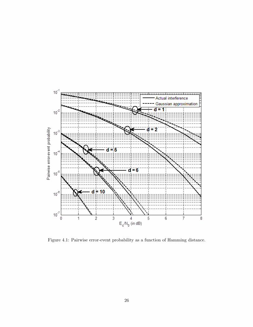
Figure 4.1: Pairwise error-event probability as a function of Hamming distance.

26

Chapter 5

Bounds on the Probability of

Code-Word Error with

Soft-Decision Viterbi Decoding

In this chapter, we describe two previously developed bounds on the probability

of code-word error for soft-decision Vitberi decoding: the concave-first-event bound and

the concave-integral bound. Both provide an upper bound on the probability of code-word

error at the output of the decoder for the system described in Chapter 2 using soft-decision

Viterbi decoding if the received signal is subjected to time-varying additive white Gaussian

noise and code-symbol interleaving. Both are used in the next chapter in conjunction with

the SGA to provide a closed-form approximation to the probability of code-word error if

the system is also subjected to multiple-access interference.

The bounds are developed in [4] utilizing results presented in [7] and [8]. A com-

parison is presented in [4] between the bounds and the probability of code-word error for

a system using convolutional coding and binary antipodal modulation. Here we extend

their use to the communication system described in Chapter 2 in which quaternary, direct-

sequence spread-spectrum modulation is used.

27

5.1 Concave-First-Event Bound

The probability of code-word error is represented by Pe. The concave-first-event

bound is expressed as

Pe ≤ 1− (1− p)L (5.1)

where p is the first-event error probability [7] at time 0 for a transmission of block length L

[4]. The first-event error probability is obtained through simulation for the specified system

and each channel of interest.

5.2 Concave-Integral Bound

The first-event union bound [4] is expressed as

Pu =1

π

∫ π2

0T (W )|W=(1−ρ)exp(−Ec

N0)+ρexp(−Ec

N1)dθ (5.2)

where T(W) is the path enumerator of the binary convolutional code [5] and the interference

activity is ρ. The parameter N0 represents the noise power spectral density when interfer-

ence is absent and the parameter N1 represents the equivalent noise plus interference power

spectral density when interference is present. The integral form of the concave bound [4] is

expressed as

Pe ≤ 1− (1− Pu)L (5.3)

where Pu is as expressed in (5.2).

28

Chapter 6

Approximation of the Performance

Using the SGA and Bounds

In this chapter we consider the system in Chapter 2 using soft-decision Viterbi de-

coding and its probability of code-word error in the presence of multiple-access interference.

We compare its performance (which is obtained by Monte Carlo simulation) with three

approximations to the performance. In the first approximation, the effect of the multiple-

access interference on each receiver statistic is approximated by a Gaussian interference

term (i.e., the SGA is used) and the performance of the approximating system is evaluated

by simulation. The second approximation is obtained by applying the concave-first-event

bound of Chapter 5 to the system with the SGA. The first-event error probability required

for the bound is obtained by Monte Carlo simulation of the system with the SGA. The

third approximation is obtained by applying the concave-integral bound of Chapter 5 to

the system with the SGA.

As examples in this chapter, we consider systems using three rate-1/2 convolutional

encoders: the memory-order-two encoder with G = (7, 5) (octal representation [5]) and

dmin = 5, the memory-order-three encoder with G = (13, 15) and dmin = 6, and the

memory-order-six CCSDS (NASA standard) encoder [9] with G = (171, 133) and dmin = 10.

The information block-length L is 1000 information bits and tail bits so that each code word

29

contains 2000 binary code symbols. Each system uses a 50 × 40 rectangular interleaver at

the transmitter and a 50 × 40 rectangular deinterleaver at the receiver. The concave-integral

bound requires the path enumerator for the convolutional code under consideration. The

path enumerators for the memory-order-two and memory-order-three codes are determined

easily using Mason’s theorem [5], and the path enumerator T(W) for the rate-1/2, NASA

standard code is given in [10].

6.1 Accuracy of the Approximations

The accuracy of each approximation to the probability of code-word error is exam-

ined in this section by considering examples with the three convolutional codes noted above

and three values of the interference activity: ρ = 0, ρ = 0.5, and ρ = 1. A single interfering

signal is considered that is chip synchronous and phase synchronous with the desired signal.

(Thus, K = 2.) There are 31 quaternary chips per binary channel symbol so that N = 31.

The interfering signal arrives at the signal with the same power as the desired signal. In

each example, the performance of the actual system and the performance of the system

using the SGA are so close that the graphs are indiscernible on the scale used in the figures.

Consequently, the graph for the simulated system using the SGA is not included in any of

the figures.

The performance of the system with an encoder of memory order of two is shown in

Figures 6.1, 6.2, and 6.3 for different values of ρ. The performance of the memory-order-two

system with no interference (i.e. ρ = 0) is shown in Figure 6.1. The concave-first-event

bound closely matches the actual probability of code-word error. It is accurate to within

0.1 dB if the probability of code-word error is 10−3 or greater. The concave-integral bound

is looser than the concave-first-event bound. It differs from the actual probability of error

by as much as 1.5 dB for some values of the probability of error greater than 10−3 and by

0.6 dB if Pe = 10−3.

The probability of code-word error of the memory-order-two system with an inter-

30

ference activity of one-half (ρ = 0.5) is shown in Figure 6.2. The concave-first-event bound

again closely matches the actual probability of code-word error obtained by simulation.

The difference is within 0.2 dB if the probability of code-word error is 10−3 or greater. The

concave-integral bound once again differs from the actual probability of error by as much

as 1.5 dB if Pe ≥ 10−3 and by 0.55 dB if Pe = 10−3.

Figure 6.3 illustrates the performance and the bounds for the memory-order-two

system if interference is present throughout the transmission (i.e., ρ = 1). The concave-

first-event bound again provides a close estimate of the actual probability of code-word

error. The difference is within 0.35 dB if the probability of code-word error is 10−3 or

greater. The concave-integral bound once again differs from the actual probability of error

by as much as 1.5 dB if Pe ≥ 10−3 and by 0.5 dB if Pe = 10−3. Thus it is seen that the

concave-first-event bound provides a very accurate approximation of the performance of

the memory-order-two system regardless of the interference activity of the channel. The

accuracy of concave-integral bound is poorer than the concave-first-event bound. However,

its accuracy improves as the probability of error decreases.

The performance of the system with an encoder of memory order of three is shown

in Figures 6.4, 6.5, and 6.6 for different values of ρ. The performance of the memory-order-

three system with no interference is shown in Figure 6.4. The concave-first-event bound

closely matches the actual probability of code-word error. It is accurate to within 0.1 dB

if the probability of code-word error is 10−3 or greater. The concave-integral bound differs

from the actual probability of error by as much as 1.5 dB for some values of the probability

of error greater than 10−3 and by 0.6 dB if Pe = 10−3.

The probability of code-word error of the memory-order-three system with an in-

terference activity of one-half is shown in Figure 6.5. The concave-first-event bound again

closely matches the actual probability of code-word error obtained by simulation, though

they differ by as much as 0.2 dB for some values of the probability of code-word error greater

than 10−3. The concave-integral bound once again differs from the actual probability of

error by as much as 1.5 dB if Pe ≥ 10−3 and by 0.55 dB if Pe = 10−3.

31

Figure 6.6 illustrates the performance and the bounds for the memory-order-three

system if interference is present throughout the transmission. The concave-first-event bound

again provides a close estimate of the actual probability of code-word error. It is accurate

to within 0.35 dB if the probability of code-word error is 10−3 or greater. The concave-

integral bound once again differs from the actual probability of error by as much as 1.5 dB

if Pe ≥ 10−3 and by 0.5 dB if Pe = 10−3. The relationship between either bound and the

actual probability of error is similar to that observed with the system of memory order two.

The performance of the system with the NASA-standard encoder (with a memory

order of six) is shown in Figures 6.7, 6.8, and 6.9 for different values of ρ. The performance

of the memory-order-six system with no interference is shown in Figure 6.7. The concave-

first-event bound closely matches the actual probability of code-word error. It is accurate to

within 0.2 dB if the probability of code-word error is 10−3 or greater. The concave-integral

bound differs from the actual probability of error by as much as 1.5 dB for some values of

the probability of error greater than 10−3, the difference is 0.65 dB if Pe = 10−2, and it is

0.55 dB if Pe = 10−3.

The probability of code-word error of the memory-order-six system with an interfer-

ence activity of one-half is shown in Figure 6.8. The concave-first-event bound again closely

matches the actual probability of code-word error obtained by simulation, differing by 0.35

dB or less if the probability of code-word error is greater than 10−3. The concave-integral

bound differs from the actual probability of error by as much as 1.5 dB for some values of

the probability of error greater than 10−3, but it differs from the actual probability of error

by only 0.55 dB if Pe = 10−2 and by 0.5 dB if Pe = 10−3.

Figure 6.9 illustrates the performance and the bounds for the memory-order-six

system if interference is present throughout the transmission. The concave-first-event bound

again provides a close estimate of the actual probability of code-word error. It is accurate

to within 0.5 dB if the probability of code-word error is 10−3 or greater. The concave-

integral bound once again differs from the actual probability of error by as much as 1.5

dB if Pe ≥ 10−3 but the difference is only 0.4 dB if Pe = 10−2 and 0.25 dB if Pe = 10−3.

32

The relationship between either bound and the actual probability of error is similar to that

observed with the systems of memory orders two and three.

In all of the examples, the concave-first-event bound closely matches the actual

probability of code-word error obtained by simulation. The concave-integral bound provides

a looser bound on the probability of code-word error: in all the cases, the concave-first-event

bound is strictly tighter than the concave-integral bound. Both bounds are more accurate

if the channel is good than if it is bad; that is, their tightness increases as the probability

of code-word error is decreased.

In other respects, the two bounds behave in a contrary manner. The tightness

of the concave-integral bound improves as the interference activity, ρ, increases, however,

whereas the tightness of the concave-first-event bound declines slightly as ρ increases. Sim-

ilarly, the concave-first-event bound is slightly less accurate with a better code than with

a weaker code, whereas the accuracy of the concave-integral bound improves noticeably as

the memory order (and minimum Hamming distance) of the code is increased.

33

Figure 6.1: Comparison of bounds for memory-order-two encoder (ρ=0).

34

Figure 6.2: Comparison of bounds for memory-order-two encoder (ρ=0.5).

35

Figure 6.3: Comparison of bounds for memory-order-two encoder (ρ=1).

36

Figure 6.4: Comparison of bounds for memory-order-three encoder (ρ=0).

37

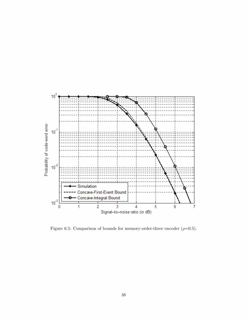
Figure 6.5: Comparison of bounds for memory-order-three encoder (ρ=0.5).

38

Figure 6.6: Comparison of bounds for memory-order-three encoder (ρ=1).

39

Figure 6.7: Comparison of bounds for NASA-standard encoder (ρ=0).

40

Figure 6.8: Comparison of bounds for NASA-standard encoder (ρ=0.5).

41

Figure 6.9: Comparison of bounds for NASA-standard encoder (ρ=1).

42

Chapter 7

Conclusion

The standard Gaussian approximation to multiple-access interference provides an

accurate approximation to the performance of a communication system using convolutional

coding, binary direct-sequence spread-spectrum modulation with quaternary spreading, and

soft-decision Viterbi decoding. The first and second moments of interference terms in the

receiver statistics are determined in the thesis using an approach similar to one used previ-

ously to determine the analogous moments for a system employing quaternary modulation

with quaternary spreading. The moments of the interference terms provide the basis for

a simulation-based approximation to the system performance and the concave-first-event

bound and the concave-integral bound on the system performance.

Using several examples of convolutional codes and considering different multiple-

access interference environments, it is shown in the thesis that the SGA yields a simulation-

based probability of code-word error than is indistinguishable from the simulation-based

probability of code-word error for actual system with multiple-access interference. The use

of the SGA with the concave-first-event bound, which is a simulation-assisted closed-form

bound, is shown to provide an approximation of the actual system’s performance that is

highly accurate. (The two are in agreement within 0.5 dB in all examples that are considered

in the thesis and within 0.2 dB in most instances.) The SGA used in conjunction with the

concave-integral bound provides an approximation of the actual system’s performance that

43

is accurate to within 1.5 dB in all of the examples considered in the thesis, and its accuracy

improves (especially for lower error probabilities) as the minimum Hamming distance of the

convolutional code is increased.

The results in the thesis provide support for the use of the SGA to reduce the compu-

tational burden in the Monte Carlo simulation of the performance in a packet-radio network

using direct-sequence spread-spectrum modulation and convolutional coding. Offline sim-

ulation of link performance for a Gaussian channel and different signal-to-noise-ratios can

provide lookup tables of high accuracy for the network simulation even though the actual

multiple-access interference in the network’s links is non-Gaussian. Moreover, the analytical

bounds based on the SGA can be used for either offline calculation or online calculation

within the network simulation to provide accurate link outcomes with low computational

burden.

44

Bibliography

[1] A. J. Viterbi, CDMA: Principles of Spread Spectrum Communication, Addison-Wesley,1995.

[2] M. B. Pursley, “The role of spread spectrum in packet radio networks,” Proceedings ofthe IEEE, vol. 75, pp. 116-134, Jan. 1987.

[3] Mohamed A. Landolsi and Wayne E. Stark, “On the Accuracy of Gaussian Approxima-tions in the Error Analysis of DS-CDMA With OQPSK Modulation,” IEEE Transac-tions on Communications, vol.50, pp. 2064 - 2071, Dec 2002.

[4] Shweta Tomar, “New Analytical Bounds on the Probability of Code-Word Error forConvolution Codes with Viterbi Decoding,” M.S. Thesis, Clemson University, 2011.

[5] S. Lin and D. J. Costello Jr., Error Control Coding, Upper Saddle River, NJ: Pearson-Prentice Hall, 2004.

[6] J. S. Lehnert and M. B. Pursley, “Error probabilities for binary direct-sequence spread-spectrum communications with random signature sequences,” IEEE Trans. Commun.,vol. COM-35, pp. 87-98, Jan. 1987.

[7] A. J. Viterbi, “Convolutional codes and their performance in communication systems,”IEEE Transactions on Communications, vol. COM-19, pp. 751-772, Oct. 1971.

[8] D. Slepian, “The one-sided barrier problem for Gaussian noise,” Bell System TechnicalJournal, vol. 41, pp. 463-501, 1962.

[9] Consultative Committee for Space Data Systems, “TM synchronization and channelcoding - summary of concept and rationale,” Green Book, vol. CCSDS, pp. 130.1-G-2,issue 2, Nov. 2012.

[10] I. M. Onyszchuk, “On the performance of convolutional codes,” Ph.D. dissertation,California Institute of Technology, 1990.

45