Embed Size (px)
Citation preview
HAL Id: hal-00757323https://hal.archives-ouvertes.fr/hal-00757323v4
Submitted on 21 Feb 2014
HAL is a multi-disciplinary open accessarchive for the deposit and dissemination of sci-entific research documents, whether they are pub-lished or not. The documents may come fromteaching and research institutions in France orabroad, or from public or private research centers.
L’archive ouverte pluridisciplinaire HAL, estdestinée au dépôt et à la diffusion de documentsscientifiques de niveau recherche, publiés ou non,émanant des établissements d’enseignement et derecherche français ou étrangers, des laboratoirespublics ou privés.
Distributed under a Creative Commons Attribution| 4.0 International License
Multiple Tests based on a Gaussian Approximation ofthe Unitary Events method with delayed coincidence
countChristine Tuleau-Malot, Amel Rouis, Franck Grammont, Patricia
Reynaud-Bouret
To cite this version:Christine Tuleau-Malot, Amel Rouis, Franck Grammont, Patricia Reynaud-Bouret. Multiple Testsbased on a Gaussian Approximation of the Unitary Events method with delayed coincidence count.Neural Computation, Massachusetts Institute of Technology Press (MIT Press), 2014, pp.1408-1454.10.1162/NECO_a_00604. hal-00757323v4

1
Multiple tests based on a Gaussian approximationof the Unitary Events method with delayed coinci-dence count
Christine Tuleau-Malot
Univ. Nice Sophia Antipolis, CNRS, LJAD, UMR 7351, 06100 Nice, France
Amel Rouis
Centre Hospitalier Universitaire de Nice, France
Franck Grammont 1
Univ. Nice Sophia Antipolis, CNRS, LJAD, UMR 7351, 06100 Nice, France
Patricia Reynaud-Bouret
Univ. Nice Sophia Antipolis, CNRS, LJAD, UMR 7351, 06100 Nice, France
Keywords: Unitary Events - Multiple Shift - Synchronization - Multiple testing -
Independence tests - Poisson processes - Neuronal assemblies
The Unitary Events (UE) method is one of the most popular and efficient methods
used this last decade to detect patterns of coincident joint spike activity among
simultaneously recorded neurons. The detection of coincidences is usually based
on binned coincidence count (Grun, 1996), which is known to be subject to loss in
synchrony detection (Grun et al., 1999). This defect has been corrected by the mul-
tiple shift coincidence count (Grun et al., 1999). The statistical properties of this
count have not been further investigated until the present work, the formula being
more difficult to deal with than the original binned count. First of all, we propose
1Corresponding author
a new notion of coincidence count, the delayed coincidence count which is equal to
the multiple shift coincidence count when discretized point processes are involved
as models for the spike trains. Moreover, it generalizes this notion to non dis-
cretized point processes, allowing us to propose a new Gaussian approximation of
the count. Since unknown parameters are involved in the approximation, we per-
form a plug-in step, where unknown parameters are replaced by estimated ones,
leading to a modification of the approximating distribution. Finally the method
takes the multiplicity of the tests into account via a Benjamini and Hochberg ap-
proach (Benjamini & Hochberg, 1995), to guarantee a prescribed control of the
false discovery rate. We compare our new method, called MTGAUE for multi-
ple tests based on a Gaussian approximation of the Unitary Events, and the UE
method proposed in (Grun et al., 1999) over various simulations, showing that
MTGAUE extends the validity of the previous method. In particular, MTGAUE
is able to detect both profusion and lack of coincidences with respect to the in-
dependence case and is robust to changes in the underlying model. Furthermore
MTGAUE is applied on real data.
1 Introduction
The study of how neural networks transmit activity in the brain and somehow code
information implies to consider various aspects of spike activity. Historically, firing
rates have been firstly considered as the main way for neurons or populations of neurons
to transmit activity, in correlation with some experimental or behavioral events. Such
kinds of correlations have been shown mainly by the use of peristimulus time histogram
(PSTH) (Abeles, 1982; Gerstein & Perkel, 1969; Shinomoto, 2010).
However, beside the role of firing rate, it has been argued, first in theoretical stud-
ies, that the activity of ensemble of neurons may be coordinated in the spatiotemporal
domain (i.e. coordination of the occurrence of spikes between different neurons) to
form neuronal assemblies (Hebb, 1949; Palm, 1990; Sakurai, 1999; Von der Malsburg,
1981). Indeed, such assemblies could be constituted on the basis of specific spike tim-
ing, thanks to several mechanisms at the synaptic level (Konig et al., 1996; Rudolph
& Destexhe, 2003; Softky & Koch, 1993). The required neural circuitry could spon-
taneously emerge with spike-timing-dependent plasticity (Brette, 2012). Such coordi-
nated activity could easily propagate over neural networks (Abeles, 1991; Diesmann
et al., 1999; Goedeke & Diesmann, 2008) and be used as a potential ”code” for the
brain (Singer, 1993, 1999). Moreover simulation studies have shown how synchroniza-
tion emerges and propagates in neural networks, with or without oscillations (Diesmann
et al., 1999; Golomb & Hansel, 2000; Tiesinga & Sejnowski, 2004; Goedeke & Dies-
mann, 2008; Rudolph & Destexhe, 2003).
2
In addition to these theoretical considerations, many experimental evidences have
been accumulated, which show that coordination between neurons is indeed taking
place. In particular, it has been shown that the mechanisms of spike generation can
be very precise (Mainen & Sejnowski, 1995) under physiological conditions (Boucsein
et al., 2011; Konishi et al., 1988; Lestienne, 2001; Prescott et al., 2008). Spike synchro-
nization, with or without oscillations, has been shown to be involved in the so-called
binding problem (Engel & Singer, 2001; Singer & Gray, 1995; Singer, 1999; Super
et al., 2003). Spike synchronization has also been studied in relation with firing rate
(Abeles & Gat, 2001; Eyherabide et al., 2009; Gerstein, 2004; Grammont & Riehle,
1999, 2003; Heinzle et al., 2007; Konig et al., 1996; Kumar et al., 2010; Lestienne,
1996; Maldonado et al., 2000; Masuda & Aihara, 2007; Riehle et al., 1997; Vaadia
et al., 1995).
Most of these experimental evidences could not have been obtained without the de-
velopment of specific descriptive analysis methods of spike-timing over the last decades:
cross-correlogram (Perkel et al., 1967), gravitational clustering (Gerstein & Aertsen,
1985) or joint peristimulus time histogram (JPSTH) (Aertsen et al., 1989). However,
these methods do not necessarily answer to a major criticism that considers that spike
synchronization might just be an epiphenomenon of the variations of the firing rate.
That is why, in direct line with these methods, Grun and collaborators developed the
Unitary Events (UE) analysis method (Grun, 1996).
The UE method is originally based on a binned coincidence count (see also Section
2.1 for a more precise definition). This method has been continuously improved until
today (Grun et al., 2002a,b; Grun, 2009; Grun et al., 2010; Gutig et al., 2001; Grun
et al., 2003; Pipa & Grun, 2003; Pipa et al., 2003; Louis et al., 2010; Pipa et al., 2013).
It is a popular method which has been used successfully in several experimental studies
(Riehle et al., 1997, 2000; Grammont & Riehle, 1999, 2003; Maldonado et al., 2008;
Kilavik et al., 2009). However, these approaches suffer from several defects due to
the use of binned coincidence count. Indeed, as pointed out in (Grun et al., 1999,
2010), there may be, for instance, a large loss in synchrony detection, coincidences
being discarded when they correspond to two spikes lying in two adjacent distinct bins.
Actually, up to 60% of the coincidences can be lost when the bin length is the typical
delay/jitter between two spikes participating to the same coincidence. Another version
of the UE method has consequently been proposed: the multiple shift coincidence count
(Grun et al., 1999) (see Section 2.1 for precise definitions, see also (Pazienti, 2008) for
another development). However, and up to our knowledge, this notion has not been
as well explored as the notion of binned coincidence count. Indeed and as already
pointed out in (Grun et al., 2010), the various shifts can make the coincidence count
more complex than a sum of independent variables, depending on the underlying model.
Therefore the main aim of this article is to complete the study of this notion of mul-
3

tiple shift coincidence count and to propose a new method which extends the validity
of the original multiple shift UE method (Grun et al., 1999). To do so, we focus on the
symmetric multiple shift coincidence count, which is much more adapted to the pur-
pose of testing independence between two spike trains on a given window (see Section
2.1 for the distinction between symmetric and asymmetric multiple shift coincidence
count). Then we generalize the notion, that was given for discretized spike trains at a
certain resolution level. The delayed coincidence count defined in Section 2.3 is exactly
the same coincidence count for discretized spike trains but this new formula can now
be also applied to non discretized point processes as well. This mathematical notion
allows us to compute the expectation and the variance in the simplest case of Poisson
processes, which approximate Bernoulli processes used in (Grun et al., 1999). There-
fore the Fano’s factor can be derived for the symmetric multiple shift / delayed coinci-
dence count, as it has been done for instance in (Pipa et al., 2013) for the more classical
notion of binned coincidence count. This also leads to a Gaussian approximation of the
distribution of the symmetric multiple shift / delayed coincidence count, when Poisson
or Bernoulli processes are involved as models for the spike trains.
However this approximation depends on unknown parameters in practice, namely
the underlying firing rates. Such problems due to unknown parameters can be bypassed
by several methods, mainly based on surrogate data (see (Louis et al., 2010) for dither-
ing or (Grun, 2009) for a more general review). On the binned coincidence count, there
are two main methods that can be easily statistically interpreted: trial-shuffling (Pipa &
Grun, 2003; Pipa et al., 2003), which is a permutation resampling method and condi-
tional distributions (Gutig et al., 2001). However trial-shuffling has in this case clearly
non trivial and specific implementation solutions and when working conditionally to the
observed number of spikes (Gutig et al., 2001), the solution is completely linked to the
form of the binned coincidence count and the use of Bernoulli models. Both solutions
are consequently not used here for the symmetric multiple shift/delayed coincidence
count, which is more intricate than classical binned coincidence count. We prefer to
look more carefully at the replacement of the unknown firing rates by estimated ones, a
step which is known in statistics as a plug-in step. By looking closely at the plug-in pro-
cedure, we show in Section 3.1 that it changes the variance of the asymptotic Gaussian
distribution, and, therefore, we correct the approximation to take this phenomenon into
account. Up to our knowledge, no correction due to the plug-in effect has been taken
into account even for the classical binned coincidence count. The last step (Section
3.2) of our procedure consists in carefully controlling the false discovery rate (FDR),
when several windows of analysis are considered, by using Benjamini and Hochberg
procedure (Benjamini & Hochberg, 1995).
Each time a thorough simulation study shows the actual performance of our proce-
dure. An analysis of real data is also performed in Section 4 on data that have already
4

been partially published, so that the detection ability of the method can be demonstrated
in concrete situations. Finally, we discuss the overall improvements due to our proce-
dure with respect to the original method of (Grun et al., 1999) in Section 5.
In all the sequel, we write in italic technical expressions, the first time they are en-
countered and we give in the same paragraph their definition. We also use the following
notation, that is the one generally used in point process theory (Daley & Vere-Jones,
2003). A point process N is a random countable set of points (of R+ here). Each point
corresponds to the detection time of a spike of the considered neuron by the recording
electrode. For any set A of R+, N(A) is the number of points in A and N(dt) is the
associated point measure, that is N(dt) =∑
S∈N δS where δS is the Dirac measure at
the point S. This means that for every function f ,∫
f(t)N(dt) =∑
S∈N f(S). The
point process corresponding to the spike train of neuron j is denoted Nj and when M
trials are recorded, the point process corresponding to the spike train of neuron j during
trial m is denoted N(m)j . In all the sequel and whatever the chosen model, we assume
that the M trials are independent and identically distributed (i.i.d.), which means er-
godicity across the trials, except when precisely stated otherwise. We denote by P the
probability measure, by E its corresponding expectation and by Var its corresponding
variance. Also 1A denotes the indicator function of the event A, which takes value 1
when A is true and 0 otherwise. Hence a function γ × 1A takes value γ on A and 0 on
the complementary event Ac.
Fundamental notions for the present article are given in the following definition (see
also (Staude et al., 2010) for this kind of distinction).
Definition 1: Real single unit data are recorded with a certain resolution h, which
is usually 10−3s or 10−4s depending on the experiment. Formally time is cut into
intervals of length h and of the form [ih − h/2, ih + h/2). Then one associates to
any point process, N , its associated sequence at resolution h, i.e. a sequence of 0
and 1, (Hn)n, where Hi = 1 corresponds to the presence of (at least) one point of
N in [ih − h/2, ih + h/2) (see also Figure 1.A). Reciprocally, to a sequence of 0
and 1, (Hn)n, we associate a point process N by taking the set of all points of the
type S = ih such that Hi = 1. Such point process that is forced to have only points
of the type ih, for some integer i, is called discretized at resolution h.
2 Probabilistic study of the coincidence count
2.1 The multiple shift coincidence count
A pair of neurons being recorded, the question is how to properly define a coincidence
and more precisely, the coincidence count. Usually those counts are computed over
5
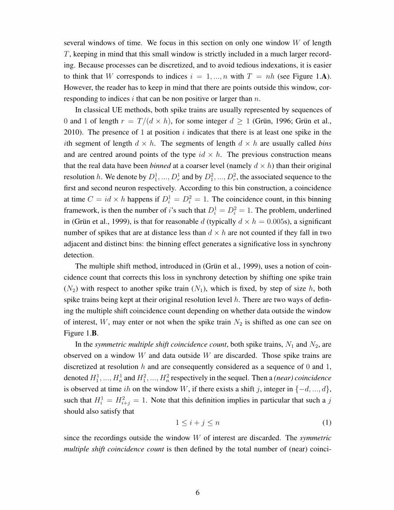
several windows of time. We focus in this section on only one window W of length
T , keeping in mind that this small window is strictly included in a much larger record-
ing. Because processes can be discretized, and to avoid tedious indexations, it is easier
to think that W corresponds to indices i = 1, ..., n with T = nh (see Figure 1.A).
However, the reader has to keep in mind that there are points outside this window, cor-
responding to indices i that can be non positive or larger than n.
In classical UE methods, both spike trains are usually represented by sequences of
0 and 1 of length r = T/(d × h), for some integer d ≥ 1 (Grun, 1996; Grun et al.,
2010). The presence of 1 at position i indicates that there is at least one spike in the
ith segment of length d × h. The segments of length d × h are usually called bins
and are centred around points of the type id × h. The previous construction means
that the real data have been binned at a coarser level (namely d× h) than their original
resolution h. We denote by D11, ..., D
1r and by D2
1, ..., D2r , the associated sequence to the
first and second neuron respectively. According to this bin construction, a coincidence
at time C = id × h happens if D1i = D2
i = 1. The coincidence count, in this binning
framework, is then the number of i’s such that D1i = D2
i = 1. The problem, underlined
in (Grun et al., 1999), is that for reasonable d (typically d × h = 0.005s), a significant
number of spikes that are at distance less than d × h are not counted if they fall in two
adjacent and distinct bins: the binning effect generates a significative loss in synchrony
detection.
The multiple shift method, introduced in (Grun et al., 1999), uses a notion of coin-
cidence count that corrects this loss in synchrony detection by shifting one spike train
(N2) with respect to another spike train (N1), which is fixed, by step of size h, both
spike trains being kept at their original resolution level h. There are two ways of defin-
ing the multiple shift coincidence count depending on whether data outside the window
of interest, W , may enter or not when the spike train N2 is shifted as one can see on
Figure 1.B.
In the symmetric multiple shift coincidence count, both spike trains, N1 and N2, are
observed on a window W and data outside W are discarded. Those spike trains are
discretized at resolution h and are consequently considered as a sequence of 0 and 1,
denoted H11 , ..., H
1n and H2
1 , ..., H2n respectively in the sequel. Then a (near) coincidence
is observed at time ih on the window W , if there exists a shift j, integer in −d, ..., d,
such that H1i = H2
i+j = 1. Note that this definition implies in particular that such a j
should also satisfy that
1 ≤ i+ j ≤ n (1)
since the recordings outside the window W of interest are discarded. The symmetric
multiple shift coincidence count is then defined by the total number of (near) coinci-
6

A: Discretization of a spike train
time
Window W
h/2 nh+h/2h/2-dh nh+h/2+dh
Window Wd
x x x x xx x x x x
x = spike
Non discretized spike train N
Associated sequence
of N on W1 1 00 1 0
Associated sequence
of N on Wd1 1 1 0 1 0 1 0 1 0
B: Multiple Shift coincidence count (d=2)
Symmetric Asymmetric
N1 on W
N2 on W
Shift of N2
j=0
j=1
j=-1
j=2
j=-2
N1 on W
N2 on Wd
1 0 1 0 1 0
1 1 0 0 0 0
1 1 0 0 0 0
1 1 0 0 0 0
1 1 0 0 0 0
1 1 0 0 0 0
1 0 1 0 1 0
1 1 0 0 0 0
1 1 0 0 0 0
1 1 0 0 0 0
1 1 0 0 0 0
1 1 0 0 0 0 1
1
1
1
1 1
1
1
1
1
1 0
1 0
1 0
1 0
1 0
C: Interpretation in term of delay
Symmetric Asymmetric
1 0 1 0 1 0
1 1 0 0 0 0
1 0 1 0 1 0
1 11 0 0 0 0 0 1 1
4 coincidences 6 coincidences
N1 on W
N2 on W N2 on Wd
N1 on W
Figure 1: Discretization and multiple shift coincidence count. In A, illustration of the
discretization of a spike train on the window W and on the enlarged window Wd. In B,
illustration of both symmetric and asymmetric multiple shift coincidence counts. In C,
interpretation of those notions in term of delay: an edge corresponds to a couple (i, k),
where i (resp. k) is the position of a 1 in the first (resp. second) spike train, and for
which the delay |i − k| is less than d. The number of coincidences is then the number
of edges. In grey are represented data that are outside W but inside Wd and that are
therefore taken into account in the asymmetric notion but not in the symmetric one.
7

dences on the window W , i.e. formally speaking
X =n
∑
i=1
∑
j/|j|≤d and 1≤i+j≤n
1H1i =H2
i+j=1. (2)
Taking k = i+ j in the previous sum, we obtain
X =n
∑
i=1
n∑
k=1
1|k−i|≤d1H1i =11H2
k=1. (3)
Hence, it can be also understood as the total number of couples (i, k) such that H1i =
H2k = 1, such that the delay |k − i| ≤ d and such that both i and k belong to 1, ..., n.
Both i and k correspond to a spike in the window of interest W : this present notion is
therefore symmetric in the first and second spike trains (see Figure 1.C).
If condition (1) is not fulfilled and if j is free, then when the shift is performed, data
outside of W ”enter” and interact with data inside W (see Figure 1.B). This leads to the
asymmetric multiple shift coincidence count, formally defined as follows
Xa =n
∑
i=1
∑
j/|j|≤d
1H1i =H2
i+j=1. (4)
Taking k = i+ j in the previous sum, we obtain this time
Xa =n
∑
i=1
∑
k∈Z
1|k−i|≤d1H1i =11H2
k=1 =
n∑
i=1
n+d∑
k=1−d
1|k−i|≤d1H1i =11H2
k=1. (5)
Hence, it can be also understood as the total number of couples (i, k) such that H1i =
H2k = 1, such that the delay |k− i| ≤ d, such that i (in 1, ..., n) corresponds to a spike
of N1 in W and such that k (in 1 − d, ..., n + d) corresponds to a spike of N2 in the
enlarged window Wd = y = x+u, x ∈ W,u ∈ [−dh, dh]. Note that with h = 10−3s,
it is quite usual to have n = 100 and up to d = 20. Hence, in the asymmetric notion,
one sequence can be 40% larger than the other one.
In the original Matlab code of (Grun et al., 1999), coincidences, i.e. couples (i, k)
such that |k − i| ≤ d, were identified at first and indexed by their position on the first
spike train, N1. Therefore when focusing on a given window W , all the coincidences
(i, k) for which i corresponds to a spike of the first spike train N1 in W were counted,
whatever the value of k. This is exactly the asymmetric multiple shift coincidence
count.
However, on the one hand, all coincidence counts are classically used to detect
dependence. They are compared to the distribution expected under the independence
hypothesis. Since the UE method aims at locally detecting the dependence, the inde-
pendence hypothesis is a local one, which depends on the underlying W , and which
8
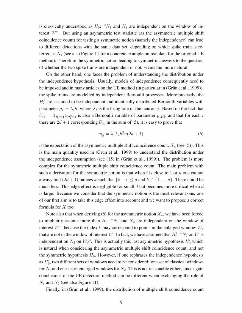
is classically understood as H0: ”N1 and N2 are independent on the window of in-
terest W ”. But using an asymmetric test statistic (as the asymmetric multiple shift
coincidence count) for testing a symmetric notion (namely the independence) can lead
to different detections with the same data set, depending on which spike train is re-
ferred as N1 (see also Figure 11 for a concrete example on real data for the original UE
method). Therefore the symmetric notion leading to symmetric answers to the question
of whether the two spike trains are independent or not, seems the more natural.
On the other hand, one faces the problem of understanding the distribution under
the independence hypothesis. Usually, models of independence consequently need to
be imposed and in many articles on the UE method (in particular in (Grun et al., 1999)),
the spike trains are modelled by independent Bernoulli processes. More precisely, the
Hji are assumed to be independent and identically distributed Bernoulli variables with
parameter pj = λjh, where λj is the firing rate of the neuron j. Based on the fact that
Uik = 1H1i =11H2
k=1 is also a Bernoulli variable of parameter p1p2, and that for each i
there are 2d+ 1 corresponding Uik in the sum of (5), it is easy to prove that
mg = λ1λ2h2n(2d+ 1), (6)
is the expectation of the asymmetric multiple shift coincidence count, Xa (see (5)). This
is the main quantity used in (Grun et al., 1999) to understand the distribution under
the independence assumption (see (15) in (Grun et al., 1999)). The problem is more
complex for the symmetric multiple shift coincidence count. The main problem with
such a derivation for the symmetric notion is that when i is close to 1 or n one cannot
always find (2d+ 1) indices k such that |k − i| ≤ d and k ∈ 1, ..., n. There could be
much less. This edge effect is negligible for small d but becomes more critical when d
is large. Because we consider that the symmetric notion is the most relevant one, one
of our first aim is to take this edge effect into account and we want to propose a correct
formula for X too.
Note also that when deriving (6) for the asymmetric notion Xa, we have been forced
to implicitly assume more than H0: ”N1 and N2 are independent on the window of
interest W ”, because the index k may correspond to points in the enlarged window Wd
that are not in the window of interest W . In fact, we have assumed that H ′0: ”N1 on W is
independent on N2 on Wd”. This is actually this last asymmetric hypothesis H ′0 which
is natural when considering the asymmetric multiple shift coincidence count, and not
the symmetric hypothesis H0. However, if one rephrases the independence hypothesis
as H ′0, two different sets of windows need to be considered: one set of classical windows
for N1 and one set of enlarged windows for N2. This is not reasonable either, since again
conclusions of the UE detection method can be different when exchanging the role of
N1 and N2 (see also Figure 11).
Finally, in (Grun et al., 1999), the distribution of multiple shift coincidence count
9

is approximated by a Poisson distribution, as it is classically done for binned coinci-
dence count, set-up where the Poisson distribution is viewed as the approximation of
a Binomial distribution. However, if it is true that the present coincidence count is a
sum of Bernoulli variables, these variables are not independent because the variable Hji
may participate in more than one coincidence, as already noted in (Grun et al., 2010).
Therefore the present multiple shift coincidence count is not a Binomial variable when
Bernoulli processes are considered. This fact makes the behavior of this precise multi-
ple shift coincidence count different from other classical notions of coincidence count
based on binning. Therefore the present work proposes a limit distribution for the coin-
cidence count that takes this dependency into account, so that the approximation is valid
for a larger set of parameters than the Poisson approximation done in (Grun et al., 1999).
If it is quite difficult to directly do so for Bernoulli processes, this probabilistic result
can be easily derived if we approximate Bernoulli processes by Poisson processes.
2.2 Bernoulli and Poisson processes
Recall that Bernoulli processes are generated as follows. For a window W of length
T , at the resolution h, n = T/h independent Bernoulli variables, Bi, with parameter
p = λh are simulated, where λ is the firing rate of the considered neuron. The associated
point process (see Definition 1) is denoted NB in the sequel.
It is well known that when h tends to 0, then the Bernoulli process tends to a Poisson
process. This can for instance be seen because the number of points, NB(W ), is a
binomial variable that tends in distribution towards a Poisson variable with parameter
λT when h tends to 0. In particular the approximation is valid as soon as n ≥ 100
and p ≤ 0.1, (Hogg & Tanis, 2009, p. 159). Since, by construction, for any disjoint
sets A1, ..., Ak, NB(A1), ..., NB(Ak) are independent variables, we recover the classical
definition of a homogeneous Poisson process of intensity λ (see (Daley & Vere-Jones,
2003) for a precise definition). Note that Poisson processes are not discretized at any
resolution level, whereas Bernoulli processes are (see Definition 1).
More precisely, in our set-up, windows of length 0.1s are classically considered,
with firing rates less than 100Hz and with resolution h = 10−3s or h = 10−4s. We are
consequently typically in a case where the Poisson approximation is valid. In (Reynaud-
Bouret et al., 2013), several classical tests, originally due to (Ogata, 1988), have been
used to test whether a point process is a homogeneous Poisson process or not and we
refer the reader to this article for detailed explanations on the procedures. In Figure 2,
10
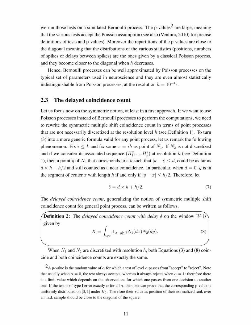
we run those tests on a simulated Bernoulli process. The p-values2 are large, meaning
that the various tests accept the Poisson assumption (see also (Ventura, 2010) for precise
definitions of tests and p-values). Moreover the repartitions of the p-values are close to
the diagonal meaning that the distributions of the various statistics (positions, numbers
of spikes or delays between spikes) are the ones given by a classical Poisson process,
and they become closer to the diagonal when h decreases.
Hence, Bernoulli processes can be well approximated by Poisson processes on the
typical set of parameters used in neuroscience and they are even almost statistically
indistinguishable from Poisson processes, at the resolution h = 10−4s.
2.3 The delayed coincidence count
Let us focus now on the symmetric notion, at least in a first approach. If we want to use
Poisson processes instead of Bernoulli processes to perform the computations, we need
to rewrite the symmetric multiple shift coincidence count in terms of point processes
that are not necessarily discretized at the resolution level h (see Definition 1). To turn
(3) into a more generic formula valid for any point process, let us remark the following
phenomenon. Fix i ≤ k and fix some x = ih as point of N1. If N2 is not discretized
and if we consider its associated sequence (H21 , ..., H
2n) at resolution h (see Definition
1), then a point y of N2 that corresponds to a k such that |k − i| ≤ d, could be as far as
d × h + h/2 and still counted as a near coincidence. In particular, when d = 0, y is in
the segment of center x with length h if and only if |y − x| ≤ h/2. Therefore, let
δ = d× h+ h/2. (7)
The delayed coincidence count, generalizing the notion of symmetric multiple shift
coincidence count for general point process, can be written as follows.
Definition 2: The delayed coincidence count with delay δ on the window W is
given by
X =
∫
W 2
1|x−y|≤δN1(dx)N2(dy). (8)
When N1 and N2 are discretized with resolution h, both Equations (3) and (8) coin-
cide and both coincidence counts are exactly the same.
2A p-value is the random value of α for which a test of level α passes from ”accept” to ”reject”. Note
that usually when α = 0, the test always accepts, whereas it always rejects when α = 1: therefore there
is a limit value which depends on the observations for which one passes from one decision to another
one. If the test is of type I error exactly α for all α, then one can prove that the corresponding p-value is
uniformly distributed on [0, 1] under H0. Therefore their value as position of their normalized rank over
an i.i.d. sample should be close to the diagonal of the square.
11
0.0 0 .2 0 .4 0 .6 0 .8 1 .0
0.0
0.2
0.4
0.6
0.8
1.0
norm alized rank
p−v
alu
es
A: Uniformity test on 2 s
0.0 0 .2 0 .4 0 .6 0 .8 1 .0
0.0
0.2
0.4
0.6
0.8
1.0
norm alized rank
p−v
alu
es
B: Uniformity test on 0.1 s
over 40 trials
0.0 0 .2 0 .4 0 .6 0 .8 1 .0
0.0
0.2
0.4
0.6
0.8
1.0
norm alized rank
p−v
alu
es
D iagona l
B ernou lli h=0 .001
B ernou lli h=0 .0001
C: Poisson test on 0.1s
over 40 trials
0.0 0 .2 0 .4 0 .6 0 .8 1 .00
.00
.20
.40
.60
.81
.0
norm alized rank
p−v
alu
es
D: Exponentiality test on 10s
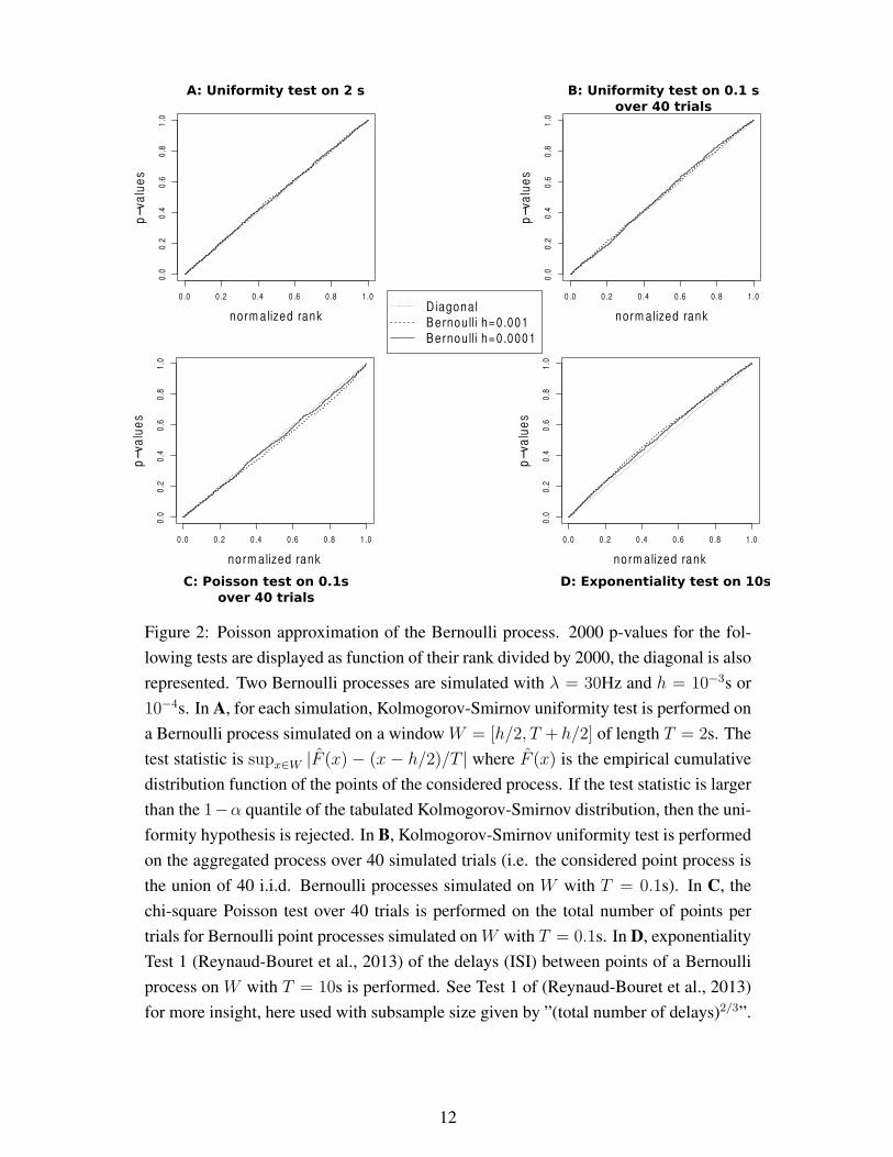
Figure 2: Poisson approximation of the Bernoulli process. 2000 p-values for the fol-
lowing tests are displayed as function of their rank divided by 2000, the diagonal is also
represented. Two Bernoulli processes are simulated with λ = 30Hz and h = 10−3s or
10−4s. In A, for each simulation, Kolmogorov-Smirnov uniformity test is performed on
a Bernoulli process simulated on a window W = [h/2, T + h/2] of length T = 2s. The
test statistic is supx∈W |F (x) − (x − h/2)/T | where F (x) is the empirical cumulative
distribution function of the points of the considered process. If the test statistic is larger
than the 1−α quantile of the tabulated Kolmogorov-Smirnov distribution, then the uni-
formity hypothesis is rejected. In B, Kolmogorov-Smirnov uniformity test is performed
on the aggregated process over 40 simulated trials (i.e. the considered point process is
the union of 40 i.i.d. Bernoulli processes simulated on W with T = 0.1s). In C, the
chi-square Poisson test over 40 trials is performed on the total number of points per
trials for Bernoulli point processes simulated on W with T = 0.1s. In D, exponentiality
Test 1 (Reynaud-Bouret et al., 2013) of the delays (ISI) between points of a Bernoulli
process on W with T = 10s is performed. See Test 1 of (Reynaud-Bouret et al., 2013)
for more insight, here used with subsample size given by ”(total number of delays)2/3”.
12
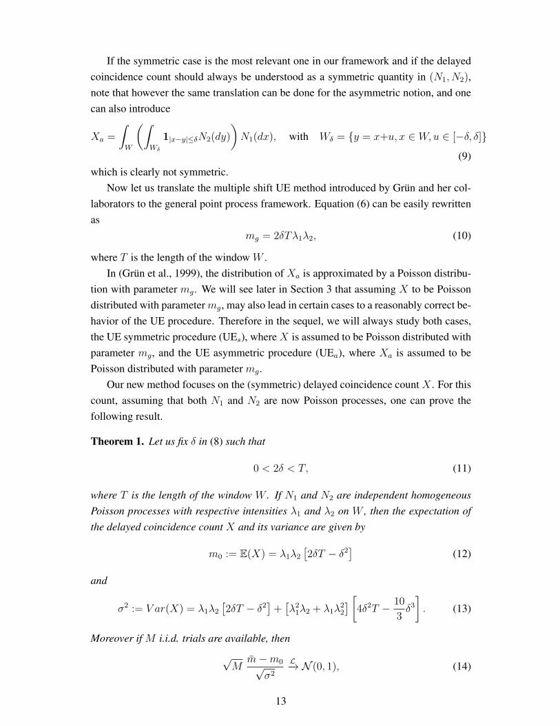
If the symmetric case is the most relevant one in our framework and if the delayed
coincidence count should always be understood as a symmetric quantity in (N1, N2),
note that however the same translation can be done for the asymmetric notion, and one
can also introduce
Xa =
∫
W
(∫
Wδ
1|x−y|≤δN2(dy)
)
N1(dx), with Wδ = y = x+u, x ∈ W,u ∈ [−δ, δ](9)
which is clearly not symmetric.
Now let us translate the multiple shift UE method introduced by Grun and her col-
laborators to the general point process framework. Equation (6) can be easily rewritten
as
mg = 2δTλ1λ2, (10)
where T is the length of the window W .
In (Grun et al., 1999), the distribution of Xa is approximated by a Poisson distribu-
tion with parameter mg. We will see later in Section 3 that assuming X to be Poisson
distributed with parameter mg, may also lead in certain cases to a reasonably correct be-
havior of the UE procedure. Therefore in the sequel, we will always study both cases,
the UE symmetric procedure (UEs), where X is assumed to be Poisson distributed with
parameter mg, and the UE asymmetric procedure (UEa), where Xa is assumed to be
Poisson distributed with parameter mg.
Our new method focuses on the (symmetric) delayed coincidence count X . For this
count, assuming that both N1 and N2 are now Poisson processes, one can prove the
following result.
Theorem 1. Let us fix δ in (8) such that
0 < 2δ < T, (11)
where T is the length of the window W . If N1 and N2 are independent homogeneous
Poisson processes with respective intensities λ1 and λ2 on W , then the expectation of
the delayed coincidence count X and its variance are given by
m0 := E(X) = λ1λ2
[
2δT − δ2]
(12)
and
σ2 := V ar(X) = λ1λ2
[
2δT − δ2]
+[
λ21λ2 + λ1λ
22
]
[
4δ2T − 10
3δ3]
. (13)
Moreover if M i.i.d. trials are available, then
√M
m−m0√σ2
L−→ N (0, 1), (14)
13

where m is the average observed coincidence count with delay δ, i.e.
m =1
M
M∑
m=1
X(m) with X(m) =
∫
W 2
1|x−y|≤δN(m)1 (dx)N
(m)2 (dy). (15)
The symbolL−→ means convergence in distribution when M tends to infinity. This
means for instance that the quantiles of√
M/σ2 (m−m0) tend to those of N (0, 1),
when M becomes larger. The proof is given in the supplementary file.
This result states first that E(X) can be computed when both observed point pro-
cesses are independent homogeneous Poisson processes and that the edge effects appear
in m0 via a quadratic term in δ which is the difference with respect to mg. Therefore it
needs to be taken into account if one wants to compute delayed coincidence count with
large δ. Note that if (11) is not satisfied, then all the couples (x, y) in W are affected by
this edge effect and in this case, the above formula for the expectation and variance are
not valid anymore.
Note also that the Fano factor3 i.e.
F :=Var(X)
E(X)= 1 + 2(λ1 + λ2)δ(1 + o(1)), (16)
is strictly larger than 1. The gap between the variable X and a Poisson variable increases
with the firing rate and with δ. Several papers have also considered the Fano factor
for binned coincidence count showing that the distribution may be different from a
Poisson distribution, but up to our knowledge nothing has been done for the multiple
shift coincidence count. In particular, in the recent (Pipa et al., 2013), Fano factors for
renewal processes are computed only in the case of a coincidence count, which is binned
but not clipped. Multiple shift coincidence count and binned clipped coincidence count
are exactly the same when the size of the bin is h for the binned coincidence count and
when d = 0 in (2) or (4) for the multiple shift symmetric or asymmetric coincidence
count. The fact that coincidence counts are clipped or not has almost no effect for
very small resolution h. Since delayed coincidence count is a generalization of the
symmetric multiple shift coincidence count, it is logical that we recover results of the
same flavour as the ones of (Pipa et al., 2013), in the Poisson case, with δ = h/2 (i.e. (7)
with d = 0). Note however that both results are not equivalent since they are not based
on the same notion of coincidence count. Using Poisson processes instead of Bernoulli
processes allows us to produce such results for the generalization of the symmetric
multiple shift coincidence count to the more general not necessarily discretized point
process case.
Note that for the asymmetric notion, one can also show that E(Xa) = mg, when
Xa is defined by (9). We will see later on simulations that Xa (discretized or not) is
3In the following equation, o(1) denotes a quantity that tends to 0 when δ tends to 0.
14
not Poisson either. Other similar computations would lead to another Gaussian approx-
imation of Xa. However we do not want to perform them and consequently correct the
asymmetric UE procedure in this way. Indeed, as stated before, the asymmetric notion
can lead to very awkward results that depend on which spike train is referred as N1,
when testing the independence hypothesis on W which is a symmetric statement (see
Figure 11 for a practical example). Even if we correct the approximation, those awk-
ward conclusions will remain and are intrinsic to the notion of asymmetric coincidence
count itself.
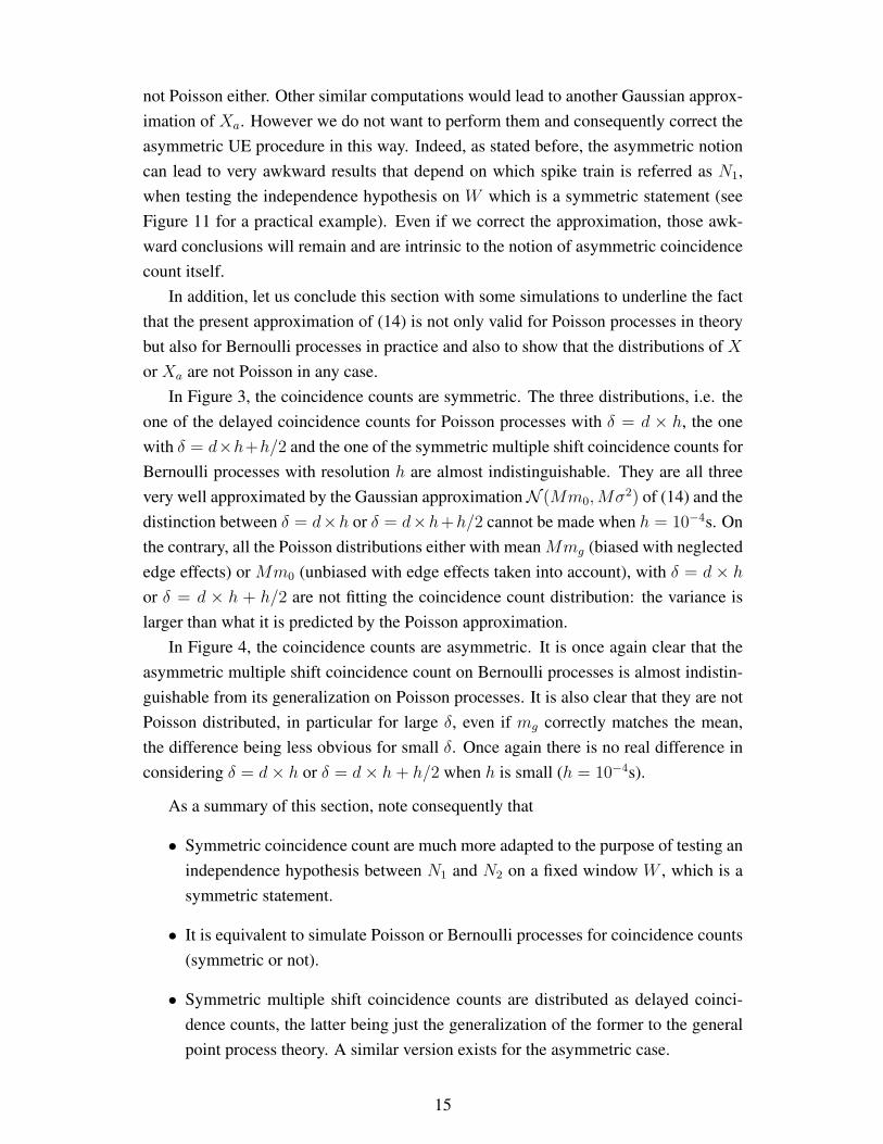
In addition, let us conclude this section with some simulations to underline the fact
that the present approximation of (14) is not only valid for Poisson processes in theory
but also for Bernoulli processes in practice and also to show that the distributions of X
or Xa are not Poisson in any case.
In Figure 3, the coincidence counts are symmetric. The three distributions, i.e. the
one of the delayed coincidence counts for Poisson processes with δ = d × h, the one
with δ = d×h+h/2 and the one of the symmetric multiple shift coincidence counts for
Bernoulli processes with resolution h are almost indistinguishable. They are all three
very well approximated by the Gaussian approximation N (Mm0,Mσ2) of (14) and the
distinction between δ = d×h or δ = d×h+h/2 cannot be made when h = 10−4s. On
the contrary, all the Poisson distributions either with mean Mmg (biased with neglected
edge effects) or Mm0 (unbiased with edge effects taken into account), with δ = d × h
or δ = d × h + h/2 are not fitting the coincidence count distribution: the variance is
larger than what it is predicted by the Poisson approximation.
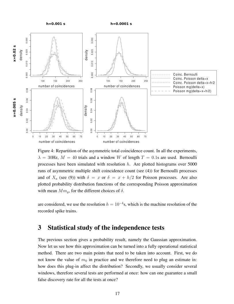
In Figure 4, the coincidence counts are asymmetric. It is once again clear that the
asymmetric multiple shift coincidence count on Bernoulli processes is almost indistin-
guishable from its generalization on Poisson processes. It is also clear that they are not
Poisson distributed, in particular for large δ, even if mg correctly matches the mean,
the difference being less obvious for small δ. Once again there is no real difference in
considering δ = d× h or δ = d× h+ h/2 when h is small (h = 10−4s).
As a summary of this section, note consequently that
• Symmetric coincidence count are much more adapted to the purpose of testing an
independence hypothesis between N1 and N2 on a fixed window W , which is a
symmetric statement.
• It is equivalent to simulate Poisson or Bernoulli processes for coincidence counts
(symmetric or not).
• Symmetric multiple shift coincidence counts are distributed as delayed coinci-
dence counts, the latter being just the generalization of the former to the general
point process theory. A similar version exists for the asymmetric case.
15

100 150 200 250
0.0
00
0.0
10
0.0
20
0.0
30
num ber o f co inc idences
de
ns
ity
h=0.001 s h=0.0001 s
x=
0.0
2 s
x=
0.0
05 s
C oinc. B ernou lliC o inc. Po isson de lta=xC o inc. Po isson de lta=x+h/2G aussian approx de lta=xG aussian approx. de lta=x+h/2Po isson m g(de lta=x)Po isson m g(de lta=x+h/2)Po isson m 0(de lta=x)Po isson m 0(de lta=x+h/2)
100 150 200 250
0.0
00
0.0
10
0.0
20
0.0
30
num ber o f co inc idencesd
en
sit
y
0 10 20 30 40 50 60 70
0.0
00
.02
0.0
40
.06
0.0
8
num ber o f co inc idences
de
ns
ity
0 10 20 30 40 50 60 70
0.0
00
.02
0.0
40
.06
0.0
8
num ber o f co inc idences
de
ns
ity
Figure 3: Repartition of the symmetric total coincidence count (i.e. the sum of the co-
incidence counts over M trials). In all the experiments, λ = 30Hz, M = 40 trials and
a window W of length T = 0.1s are used. Bernoulli processes have been simulated
with resolution h. Are plotted histograms over 5000 runs of symmetric multiple shift
coincidence count for Bernoulli processes (see (2)) and of delayed coincidence count
with δ = x or δ = x + h/2 for Poisson processes (see Definition 2). Are also plotted
densities of the corresponding Gaussian approximation as well as probability distribu-
tion functions of the corresponding Poisson approximation with mean Mmg or Mm0,
for the different choices of δ.
• In either case, the distribution is not Poisson.
• In both cases (Poisson or Bernoulli processes), the Gaussian approximation of
(14) is valid for the symmetric notion, on the classical set of parameters.
• Edge effects need to be taken into account for large δ, when dealing with the
symmetric notion of coincidence count.
• Considering δ = d × h or δ = d × h + h/2 with h = 10−4s is completely
equivalent.
Therefore, in the sequel, we use delayed coincidence count with δ of the type d×h.
Bernoulli processes are replaced by Poisson processes when necessary. When real data
16
h=0.001 s h=0.0001 s
x=
0.0
2 s
x=
0.0
05 s
100 150 200 250
0.0
00
0.0
10
0.0
20
0.0
30
num ber o f co inc idences
de
ns
ity
100 150 200 250
0.0
00
0.0
10
0.0
20
0.0
30
num ber o f co inc idencesd
en
sit
y
0 10 20 30 40 50 60 70
0.0
00
.02
0.0
40
.06
0.0
8
num ber o f co inc idences
de
ns
ity
C o inc. B ernou lliC o inc. Po isson de lta=xC o inc. Po isson de lta=x+h/2Po isson m g(de lta=x)Po isson m g(de lta=x+h/2)
0 10 20 30 40 50 60 70
0.0
00
.02
0.0
40
.06
0.0
8
num ber o f co inc idences
de
ns
ity
Figure 4: Repartition of the asymmetric total coincidence count. In all the experiments,
λ = 30Hz, M = 40 trials and a window W of length T = 0.1s are used. Bernoulli
processes have been simulated with resolution h. Are plotted histograms over 5000
runs of asymmetric multiple shift coincidence count (see (4)) for Bernoulli processes
and of Xa (see (9)) with δ = x or δ = x + h/2 for Poisson processes. Are also
plotted probability distribution functions of the corresponding Poisson approximation
with mean Mmg, for the different choices of δ.
are considered, we use the resolution h = 10−4s, which is the machine resolution of the
recorded spike trains.
3 Statistical study of the independence tests
The previous section gives a probability result, namely the Gaussian approximation.
Now let us see how this approximation can be turned into a fully operational statistical
method. There are two main points that need to be taken into account. First, we do
not know the value of m0 in practice and we therefore need to plug an estimate in:
how does this plug-in affect the distribution? Secondly, we usually consider several
windows, therefore several tests are performed at once: how can one guarantee a small
false discovery rate for all the tests at once?
17

3.1 Plug-in and modification of the Gaussian approximation
Equation (14) depends on m0 and σ that are unknown. Hence to perform the approx-
imation in practice, we need to replace them by corresponding estimates, based on the
observations. This step is known in statistics as a plug-in step and it is known to some-
times dramatically modify the distribution. One of the most famous example is the
Gaussian distribution which has to be replaced by a Student distribution when the vari-
ance is unknown and estimated by an empirical mean over less than 30 realizations 4
(Hogg & Tanis, 2009, Table VI, p 658).
Theoretical study
In the present set-up, as far as asymptotic in the number of trials M is concerned, the
plug-in of an estimate of σ does not change the Gaussian distribution, whereas the plug-
in of an estimate of m0 changes the variance of the limit, as we can see in the following
result.
Theorem 2. With the same notation as in Theorem 1, let λj be the unbiased estimate of
λj , the firing rate of neuron j, defined by
λj :=1
MT
M∑
m=1
N(m)j (W ). (17)
Let also m0 be an estimate of m0 defined by
m0 := λ1λ2[2δT − δ2]. (18)
Then under the assumptions of Theorem 1,
√M (m− m0)
L−→ N (0, v2), (19)
where
v2 := λ1λ2
[
2δT − δ2]
+ λ1λ2 [λ1 + λ2]
[
2
3δ3 − T−1δ4
]
. (20)
Moreover v2 can be estimated by
v2 := λ1λ2
[
2δT − δ2]
+ λ1λ2
[
λ1 + λ2
]
[
2
3δ3 − T−1δ4
]
(21)
and √M
m− m0√v2
L−→ N (0, 1). (22)
The proof is given in the supplementary file.
4More precisely, if X1, ..., Xn are i.i.d. Gaussian variables with mean m and variance σ2 then√
n/σ2∑
n
i=1(Xi − m) ∼ N (0, 1) whereas
√
n/σ2∑
n
i=1(Xi − m) ∼ T (n − 1) where σ2 is the
unbiased estimate of σ2.
18

−5 0 5 10
0.0
0.1
0.2
0.3
0.4
renorm alized num ber o f co inc idences
de
ns
ity
−5 0 5 10
0.0
0.1
0.2
0.3
0.4
−5 0 5 10
0.0
0.1
0.2
0.3
0.4
−5 0 5 10
0.0
0.1
0.2
0.3
0.4
−5 0 5 10
0.0
0.1
0.2
0.3
0.4
0.5
0.6
renorm alized num ber o f co inc idences
de
ns
ity
−5 0 5 10
0.0
0.1
0.2
0.3
0.4
0.5
0.6
−5 0 5 10
0.0
0.1
0.2
0.3
0.4
0.5
0.6
renorm alized num ber o f co inc idences
de
ns
ity
−5 0 5 10
0.0
0.1
0.2
0.3
0.4
0.5
0.6
−5 0 5 10
0.0
0.1
0.2
0.3
0.4
0.5
0.6
renorm alized num ber o f co inc idences
de
ns
ity
−5 0 5 10
0.0
0.1
0.2
0.3
0.4
0.5
0.6
−5 0 5 10
0.0
0.1
0.2
0.3
0.4
0.5
0.6
renorm alized num ber o f co inc idences
de
ns
ity
−5 0 5 10
0.0
0.1
0.2
0.3
0.4
0.5
0.6
−5 0 5 10
0.0
0.1
0.2
0.3
0.4
0.5
0.6
renorm alized num ber o f co inc idences
de
ns
ity
−5 0 5 10
0.0
0.1
0.2
0.3
0.4
0.5
0.6
−5 0 5 10
0.0
0.1
0.2
0.3
0.4
0.5
0.6
renorm alized num ber o f co inc idences
de
ns
ity
−5 0 5 10
0.0
0.1
0.2
0.3
0.4
0.5
0.6
density o f N (0 ,1 )
M σ × (m −m 0)
M v × (m − m 0)
M v × (m − m 0)
M σ × (m − m 0)
M σ × (m − m 0)
M m g × (m −m g)
M m g × (m − m g)
A: Plug-in / correct variances B: Plug-in / original variances
C: Poisson / symmetric count D: Poisson / asymmetric count
Figure 5: Repartition of the different renormalizations of the various coincidence
counts. Each time 5000 simulations of two independent Poisson processes with
λ1 = λ2 = 30Hz, M = 40 trials, a window W of length T = 0.1s and δ = 0.02s
are performed. In A, histograms of√M(m − m0)/σ, of
√M(m − m0)/v and of√
M(m − m0)/v with m the average delayed coincidence count. In B, histogram of√M(m − m0)/σ and of
√M(m − m0)/σ with m the average delayed coincidence
count. In C, histogram of√M(m−mg)/
√mg and of
√M(m− mg)/
√
mg with m the
average delayed coincidence count. In D, same thing as in C but with m, the average of
Xa (see (9)), the asymmetric coincidence count.
Figure 5 illustrates the impact of the plug-in in the renormalized coincidence count
distribution. When using plug-in, we need to renormalize the count since at each run a
new value for the estimate is drawn. Therefore our reference in Figure 5 is the standard
Gaussian variable. First we see that the Gaussian approximation of (14) is still valid,
but more importantly that the plug-in steps of (19) and (22) are valid on Figure 5.A.
Instead of the new variance v2 and its estimate v2, we have also plugged m0 in with the
original variance, σ2, or a basic estimate of σ2, namely
σ2 = λ1λ2
[
2δT − δ2]
+[
λ21λ2 + λ1λ
22
]
[
4δ2T − 10
3δ3]
. (23)
19
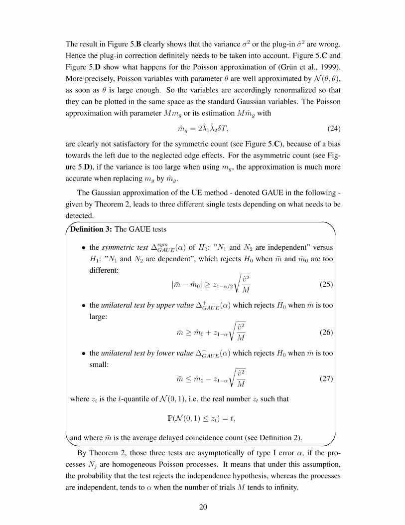
The result in Figure 5.B clearly shows that the variance σ2 or the plug-in σ2 are wrong.
Hence the plug-in correction definitely needs to be taken into account. Figure 5.C and
Figure 5.D show what happens for the Poisson approximation of (Grun et al., 1999).
More precisely, Poisson variables with parameter θ are well approximated by N (θ, θ),
as soon as θ is large enough. So the variables are accordingly renormalized so that
they can be plotted in the same space as the standard Gaussian variables. The Poisson
approximation with parameter Mmg or its estimation Mmg with
mg = 2λ1λ2δT, (24)
are clearly not satisfactory for the symmetric count (see Figure 5.C), because of a bias
towards the left due to the neglected edge effects. For the asymmetric count (see Fig-
ure 5.D), if the variance is too large when using mg, the approximation is much more
accurate when replacing mg by mg.
The Gaussian approximation of the UE method - denoted GAUE in the following -
given by Theorem 2, leads to three different single tests depending on what needs to be
detected.
Definition 3: The GAUE tests
• the symmetric test ∆symGAUE(α) of H0: ”N1 and N2 are independent” versus
H1: ”N1 and N2 are dependent”, which rejects H0 when m and m0 are too
different:
|m− m0| ≥ z1−α/2
√
v2
M(25)
• the unilateral test by upper value ∆+GAUE(α) which rejects H0 when m is too
large:
m ≥ m0 + z1−α
√
v2
M(26)
• the unilateral test by lower value ∆−GAUE(α) which rejects H0 when m is too
small:
m ≤ m0 − z1−α
√
v2
M(27)
where zt is the t-quantile of N (0, 1), i.e. the real number zt such that
P(N (0, 1) ≤ zt) = t,
and where m is the average delayed coincidence count (see Definition 2).
By Theorem 2, those three tests are asymptotically of type I error α, if the pro-
cesses Nj are homogeneous Poisson processes. It means that under this assumption,
the probability that the test rejects the independence hypothesis, whereas the processes
are independent, tends to α when the number of trials M tends to infinity.
20

The original UE multiple shift method of (Grun et al., 1999) can be formalized in
the same way.
Definition 4: The UE tests
• a symmetric test ∆symUE (α) which rejects H0 when Mm ≤ qα/2 or Mm ≥
q1−α/2
• the unilateral test by upper value ∆+UE(α) which rejects H0 when Mm ≥
q1−α
• the unilateral test by lower value ∆−UE(α) which rejects H0 when Mm ≤ qα
where qt is the t-quantile of a Poisson variable whose parameter is given by
Mmg = 2MδTλ1λ2.
Each of the previous tests exists in two versions (UEs or UEa respectively) depend-
ing on whether m is the average delayed coincidence count (symmetric notion, see
(8)) or the average Xa (asymmetric notion, see (9) ).
Up to our knowledge, no other operational method based on multiple shift coin-
cidence count has been developed. In particular, the distribution free methods such
as trial-shuffling methods developped by Pipa and collaborators, which avoid plug-in
problems, are based on binned coincidence count (Pipa & Grun, 2003; Pipa et al., 2003)
and not on multiple shift coincidence count. Plug-in effects can also be avoided in an-
other way, on binned coincidence count, by considering conditional distribution (Gutig
et al., 2001).
Simulation study on one window
The simulation study is consequently restricted to the two previous sort of tests (GAUE
and UE) to focus on this particular notion of delayed/multiple shift coincidence count,
which is drastically different from binned coincidence count.
Simulated processes Several processes have been simulated. The Poisson processes
have already been described in Section 2.2. They constitute a particular case of more
general counting processes, called the Hawkes processes, which can be simulated by
thinning algorithms (Daley & Vere-Jones, 2003; Ogata, 1981; Reimer et al., 2012). Af-
ter a brief apparition in (Chornoboy et al., 1988), they have recently been used again
to model spike trains in (Krumin et al., 2010; Pernice et al., 2011, 2012). A bivariate
Hawkes process (N1, N2) is described by its respective conditional intensities with re-
spect to the past, (λ1(.), λ2(.)). Informally, the quantity λj(t)dt gives the probability
that a new point on Nj appears in [t, t+dt] given the past. We refer the reader to (Brown
21
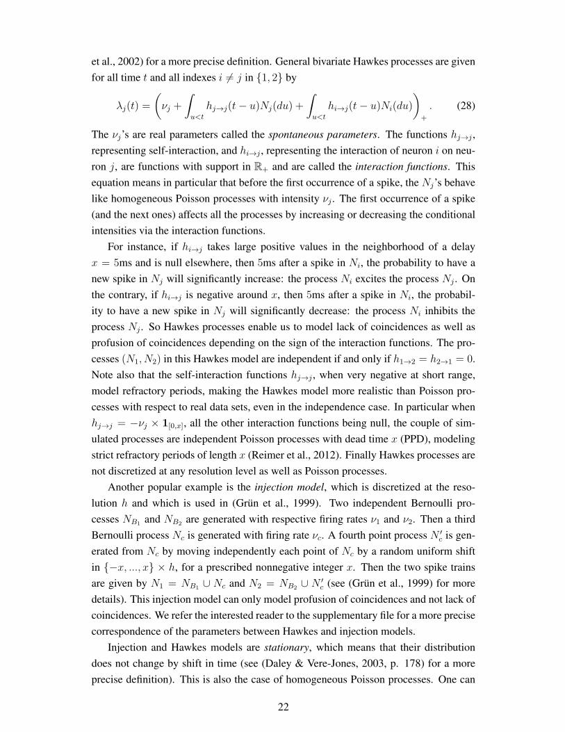
et al., 2002) for a more precise definition. General bivariate Hawkes processes are given
for all time t and all indexes i 6= j in 1, 2 by
λj(t) =
(
νj +
∫
u<t
hj→j(t− u)Nj(du) +
∫
u<t
hi→j(t− u)Ni(du)
)
+
. (28)
The νj’s are real parameters called the spontaneous parameters. The functions hj→j ,
representing self-interaction, and hi→j , representing the interaction of neuron i on neu-
ron j, are functions with support in R+ and are called the interaction functions. This
equation means in particular that before the first occurrence of a spike, the Nj’s behave
like homogeneous Poisson processes with intensity νj . The first occurrence of a spike
(and the next ones) affects all the processes by increasing or decreasing the conditional
intensities via the interaction functions.
For instance, if hi→j takes large positive values in the neighborhood of a delay
x = 5ms and is null elsewhere, then 5ms after a spike in Ni, the probability to have a
new spike in Nj will significantly increase: the process Ni excites the process Nj . On
the contrary, if hi→j is negative around x, then 5ms after a spike in Ni, the probabil-
ity to have a new spike in Nj will significantly decrease: the process Ni inhibits the
process Nj . So Hawkes processes enable us to model lack of coincidences as well as
profusion of coincidences depending on the sign of the interaction functions. The pro-
cesses (N1, N2) in this Hawkes model are independent if and only if h1→2 = h2→1 = 0.
Note also that the self-interaction functions hj→j , when very negative at short range,
model refractory periods, making the Hawkes model more realistic than Poisson pro-
cesses with respect to real data sets, even in the independence case. In particular when
hj→j = −νj × 1[0,x], all the other interaction functions being null, the couple of sim-
ulated processes are independent Poisson processes with dead time x (PPD), modeling
strict refractory periods of length x (Reimer et al., 2012). Finally Hawkes processes are
not discretized at any resolution level as well as Poisson processes.
Another popular example is the injection model, which is discretized at the reso-
lution h and which is used in (Grun et al., 1999). Two independent Bernoulli pro-
cesses NB1and NB2
are generated with respective firing rates ν1 and ν2. Then a third
Bernoulli process Nc is generated with firing rate νc. A fourth point process N ′c is gen-
erated from Nc by moving independently each point of Nc by a random uniform shift
in −x, ..., x × h, for a prescribed nonnegative integer x. Then the two spike trains
are given by N1 = NB1∪ Nc and N2 = NB2
∪ N ′c (see (Grun et al., 1999) for more
details). This injection model can only model profusion of coincidences and not lack of
coincidences. We refer the interested reader to the supplementary file for a more precise
correspondence of the parameters between Hawkes and injection models.
Injection and Hawkes models are stationary, which means that their distribution
does not change by shift in time (see (Daley & Vere-Jones, 2003, p. 178) for a more
precise definition). This is also the case of homogeneous Poisson processes. One can
22
also simulate inhomogeneous Poisson processes, which correspond to a conditional
intensity t → λ(t) which is deterministic but not constant. These inhomogeneous
Poisson processes are therefore non stationary in time (see (Daley & Vere-Jones, 2003)
for more details).
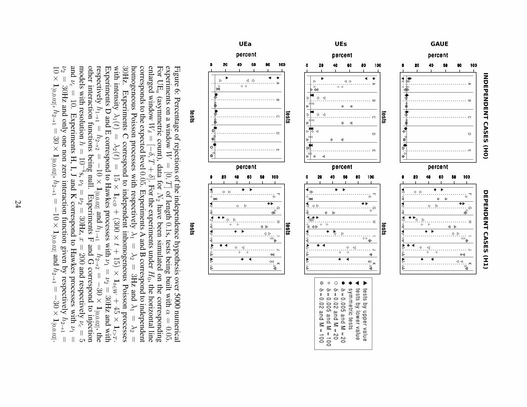
Figure 6 gives the percentage of rejections over various numerical experiments, that
have been led on those simulated processes.
Type I error Since H0 refers to ”N1 and N2 are independent on W ” (or ”N1 on W
is independent of N2 on Wδ” for UEa), we have simulated various situations of inde-
pendence. Our theoretical work proves that the level is asymptotically guaranteed if the
processes are homogeneous Poisson processes. Our aim is now twofolds: First check
whether the level is controlled for a finite, relatively small, number of trials (Experi-
ments A and B). Next check if it still holds, when the processes are not homogeneous
Poisson processes (Experiments C, D and E). Moreover we want to compare our results
to the ones of UEs and UEa. The upper left part of Figure 6 shows that the three forms
of GAUE (symmetric, upper and lower value) guarantee a level of roughly 5% and this
even for a very small number of trials (M = 20) with a very small firing rate (λ = 3Hz)
or with large δ (δ = 0.02s). In this sense, it clearly extends the validity of the original
UE method (UEa in the lower part of Figure 6), which is known to be inadequate for
firing rates less than 7Hz (Roy et al., 2000), as one can see with Experiments A. Note
also that the level for GAUE as well as for UEa seems robust to changes in the model:
non stationarity for inhomogeneous Poisson processes (Experiments C), refractory pe-
riods when using Hawkes processes (Experiments D and E). Note finally that the UEs
method does not guarantee the correct level except for the test by upper value, which is
much smaller than 5%.
Power Several dependence situations have been tested in the right part of Figure 6:
GAUE tests by upper value can adequately detect profusion of coincidences induced
by injection models (see Experiments F and G) or Hawkes models (see Experiments
H and I). GAUE tests by lower value can on the contrary detect lack of coincidences,
simulated by inhibitory Hawkes processes (see Experiments J and K). Note moreover
that symmetric GAUE tests can detect both situations. The same conclusions are true
for both UE methods, the power being of the same order as the GAUE tests except for
the injection case with low νc (Experiments F with δ = 0.02 and M = 100) where
GAUE is clearly better.
As a partial conclusion, the Gaussian approximation of Theorem 1 needs to be mod-
ified to take into account the plug-in effect. Once this modification is done (see The-
orem 2) the Gaussian approximation leads to tests that are shown to be of asymptotic
level α. Our simulation study has shown (see Figure 6) that MTGAUE type I error is
23
0 20 40 60 80 100
tes
ts
pe rcen t
0 20 40 60 80 100
tes
ts
pe rcen t
0 20 40 60 80 100
tes
ts
pe rcen t
0 20 40 60 80 100
tes
ts
pe rcen t
0 20 40 60 80 100
tes
ts
pe rcen t
0 20 40 60 80 100
tes
ts
pe rcen t
0 20 40 60 80 1000 20 40 60 80 1000 20 40 60 80 1000 20 40 60 80 1000 20 40 60 80 1000 20 40 60 80 1000 20 40 60 80 1000 20 40 60 80 1000 20 40 60 80 1000 20 40 60 80 1000 20 40 60 80 1000 20 40 60 80 1000 20 40 60 80 1000 20 40 60 80 1000 20 40 60 80 1000 20 40 60 80 1000 20 40 60 80 100
AB
CD
E
0 20 40 60 80 100
0 20 40 60 80 100
tes
ts
pe rcen t
0 20 40 60 80 100
tes
ts
pe rcen t
0 20 40 60 80 100
tes
ts
pe rcen t
0 20 40 60 80 100
tes
ts
pe rcen t
0 20 40 60 80 100
tes
ts
pe rcen t
0 20 40 60 80 100
tes
ts
pe rcen t
0 20 40 60 80 100
tes
ts
pe rcen t
0 20 40 60 80 1000 20 40 60 80 1000 20 40 60 80 1000 20 40 60 80 1000 20 40 60 80 1000 20 40 60 80 1000 20 40 60 80 1000 20 40 60 80 1000 20 40 60 80 1000 20 40 60 80 1000 20 40 60 80 1000 20 40 60 80 1000 20 40 60 80 1000 20 40 60 80 1000 20 40 60 80 1000 20 40 60 80 1000 20 40 60 80 1000 20 40 60 80 100
FG
HI
JK
0 20 40 60 80 100
tes
ts
pe rcen t
0 20 40 60 80 100
tes
ts
pe rcen t
0 20 40 60 80 100
tes
ts
pe rcen t
0 20 40 60 80 100
tes
ts
pe rcen t
0 20 40 60 80 100
ts
pe rcen t
0 20 40 60 80 100
percent
0 20 40 60 80 1000 20 40 60 80 1000 20 40 60 80 1000 20 40 60 80 1000 20 40 60 80 1000 20 40 60 80 1000 20 40 60 80 1000 20 40 60 80 1000 20 40 60 80 1000 20 40 60 80 1000 20 40 60 80 1000 20 40 60 80 1000 20 40 60 80 1000 20 40 60 80 1000 20 40 60 80 1000 20 40 60 80 1000 20 40 60 80 100
AB
CD
E
0 20 40 60 80 1000 20 40 60 80 100
tes
ts
pe rcen t
0 20 40 60 80 100
tes
ts
pe rcen t
0 20 40 60 80 100
tes
ts
pe rcen t
0 20 40 60 80 100
tes
ts
pe rcen t
0 20 40 60 80 100
tes
ts
pe rcen t
0 20 40 60 80 100
tes
ts
pe rcen t
0 20 40 60 80 1000 20 40 60 80 1000 20 40 60 80 1000 20 40 60 80 1000 20 40 60 80 1000 20 40 60 80 1000 20 40 60 80 1000 20 40 60 80 1000 20 40 60 80 1000 20 40 60 80 1000 20 40 60 80 1000 20 40 60 80 1000 20 40 60 80 1000 20 40 60 80 1000 20 40 60 80 1000 20 40 60 80 1000 20 40 60 80 100
AB
CD
E
0 20 40 60 80 100
0 20 40 60 80 100
tes
ts
pe rcen t
0 20 40 60 80 100
tes
ts
pe rcen t
0 20 40 60 80 100
tes
ts
pe rcen t
0 20 40 60 80 100
tes
ts
pe rcen t
0 20 40 60 80 100
tes
ts
pe rcen t
0 20 40 60 80 100
tes
ts
pe rcen t
0 20 40 60 80 100
tes
ts
pe rcen t
0 20 40 60 80 1000 20 40 60 80 1000 20 40 60 80 1000 20 40 60 80 1000 20 40 60 80 1000 20 40 60 80 1000 20 40 60 80 1000 20 40 60 80 1000 20 40 60 80 1000 20 40 60 80 1000 20 40 60 80 1000 20 40 60 80 1000 20 40 60 80 1000 20 40 60 80 1000 20 40 60 80 1000 20 40 60 80 1000 20 40 60 80 1000 20 40 60 80 100
FG
HI
JK
tes
ts b
y u
pp
er va
lue
tes
ts b
y lo
we
r valu
es
ym
me
tric te
sts
δ=
0.0
05
an
dM=
20
δ=
0.0
2a
nd
M=
20
δ=
0.0
05
an
dM=
10
0δ=
0.0
2a
nd
M=
10
0
IND
EP
EN
DEN
T C
AS
ES
(H0)
0 20 40 60 80 100
tes
ts
pe rcen t
0 20 40 60 80 100
tes
ts
pe rcen t
0 20 40 60 80 100
tes
ts
pe rcen t
0 20 40 60 80 100
tes
ts
pe rcen t
0 20 40 60 80 100
tes
ts
pe rcen t
0 20 40 60 80 100
tes
ts
pe rcen t
0 20 40 60 80 100
tes
ts
pe rcen t
0 20 40 60 80 1000 20 40 60 80 1000 20 40 60 80 1000 20 40 60 80 1000 20 40 60 80 1000 20 40 60 80 1000 20 40 60 80 1000 20 40 60 80 1000 20 40 60 80 1000 20 40 60 80 1000 20 40 60 80 1000 20 40 60 80 1000 20 40 60 80 1000 20 40 60 80 1000 20 40 60 80 1000 20 40 60 80 1000 20 40 60 80 1000 20 40 60 80 100
FG
HI
JK
DEP
EN
DEN
T C
AS
ES
(H1)
GAUEUEsUEa
Fig
ure
6:
Percen
tage
of
rejections
of
the
indep
enden
cehypoth
esisover
5000
num
ericalex
perim
ents
on
aw
indow
W=
[0,T]
of
length
0.1s,
testsbein
gbuilt
with
α=
0.05.
For
UEa
(asym
metric
count),
data
forN
2hav
ebeen
simulated
on
the
corresp
ondin
gen
larged
win
dowW
δ=
[−δ,T
+δ].
For
the
experim
ents
under
H0 ,
the
horizo
ntal
line
corresp
onds
toth
eex
pected
level0.05
.E
xperim
ents
Aan
dB
corresp
ond
toin
dep
enden
thom
ogen
eous
Poisso
npro
cessesw
ithresp
ectively
λ1=
λ2=
3H
zan
dλ1=
λ2=
30H
z.E
xperim
ents
Cco
rrespond
toin
dep
enden
tin
hom
ogen
eous
Poisso
npro
cessesw
ithin
tensity
λ1 (t)
=λ2 (t)
=15
×1t<
0+
(300×
t+
15)×1t∈
W+
45×
1t>
T.
Experim
ents
Dan
dE
corresp
ond
toH
awkes
pro
cessesw
ithν1=
ν2=
30H
zan
dw
ithresp
ectively
h1→
1=
h2→
2=
−10×
1[0,0.02]
andh1→
1=
h2→
2=
−30×
1[0,0.02] ,
the
oth
erin
teraction
functio
ns
bein
gnull.
Experim
ents
Fan
dG
corresp
ond
toin
jection
models
with
resolu
tionh=
10−4s,
ν1=
ν2=
30H
z,x=
200an
dresp
ectively
νc=
5an
dνc=
10.
Experim
ents
H,
I,J
and
Kco
rrespond
toH
awkes
pro
cessesw
ithν1=
ν2=
30H
zan
donly
one
non
zeroin
teraction
functio
ngiv
enby
respectiv
elyh2→
1=
10×1[0,0.02] ,h
2→
1=
30×1[0,0.02] ,h
2→
1=
−10×
1[0,0.02]an
dh2→
1=
−30×
1[0,0.02] .
24
of order 5% even for small firing rates and that those tests seem robust to variations
in the model (non stationarity, refractory periods). Moreover symmetric GAUE tests
are able to detect both profusion and lack of coincidences. Except for very small firing
rates where its level is not controlled, the original UE method (UEa) shares the same
properties, whereas the level of UEs is not controlled in any cases except for the test by
upper values.
3.2 Multiple tests and false discovery rate
Classical UE analysis (Grun, 1996; Grun et al., 1999) is performed on several windows,
so that dependence regions can be detected through time. We want to produce the same
kind of analysis with GAUE. However, since a test is by essence a random answer, it is
not true that the control of one test at level α automatically induces a controlled number
of false rejections.
Indeed, let us consider a collection W of possibly overlapping windows W , with
cardinality K and, to illustrate the problem, let us assume that we observe two indepen-
dent homogeneous Poisson processes. Now let us perform any of the previous GAUE
tests at level α on each of the previous windows. Then by linearity of the expectation,
one has that
E(number of rejections) = KP(one test rejects) →M→∞ Kα. (29)
Moreover, if L is the maximal number of disjoint windows in W , then the probability
that the K tests accept the independence hypothesis is upper bounded by
P(the L tests accept) = P(one test accepts)L →M→∞ (1− α)L →L→∞ 0, (30)
by independence of the test statistics between disjoint windows. This means that for
large M , this procedure is doomed to reject in average Kα tests and the procedure will
reject at least one test, when L grows. Consequently, one cannot apply multiple tests
procedure without correcting them for multiplicity. Ventura also underlined the problem
of the multiplicity of the tests, and proposed a procedure which is not as general as the
one described here (Ventura, 2010).
Multiple testing correction: a Benjamini and Hochberg approach
Let us denote ∆W the test considered on the window W .
One way to control multiple testing procedure based on the ∆W ’s, is to control the
so called familywise error rate (FWER) (Hochberg & Tamhame, 1987), which consists
in controlling
FWER = P(∃W ∈ W ,∆W wrongly rejects). (31)
25
This can be easily done by Bonferroni bounds:
P(∃W ∈ W ,∆W wrongly rejects) ≤∑
W∈W
P(∆W wrongly rejects) →M→∞ Kα.
(32)
So Bonferroni’s method (Holm, 1979) consists in applying the ∆W tests at level α/K
instead of α to guarantee a FWER less than α. However, the smaller the type I error, the
more difficult it is to make a rejection. Usually, the rejected tests are called detections
(or discoveries). So when K is large, Bonferroni’s procedure potentially leads to no
discovery/detection at all, even in cases where dependent structures exist.
Another notion, popularized by (Benjamini & Hochberg, 1995) has consequently been
introduced in the multiple testing areas leading to a large amount of publications in
statistics, genomics, medicine etc in the past ten years (Benjamini, 2010). This is the
false discovery rate (FDR). Actually, a false discovery (also named false detection) is
not that bad if the ratio of the number of false discoveries divided by the total number
of discoveries is small.
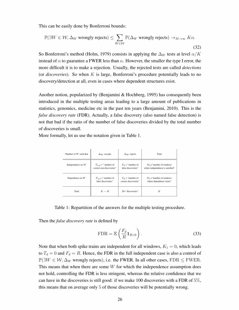
More formally, let us use the notation given in Table 1.
Number of W such that ∆W accepts ∆W rejects Total
Independence on W Tnd = ” number of Fd = ”number of K0=”number of windows
correct non discoveries” false discoveries” where independence is satisfied”
Dependence on W Fnd = ”number of Td = ”number of K1=”number of windows
false discoveries” correct discoveries” where dependence exists”
Total K − R R= ”discoveries” K
Table 1: Repartition of the answers for the multiple testing procedure.
Then the false discovery rate is defined by
FDR = E
(
Fd
R1R>0
)
. (33)
Note that when both spike trains are independent for all windows, K1 = 0, which leads
to Td = 0 and Fd = R. Hence, the FDR in the full independent case is also a control of
P(∃W ∈ W ,∆W wrongly rejects), i.e. the FWER. In all other cases, FDR ≤ FWER.
This means that when there are some W for which the independence assumption does
not hold, controlling the FDR is less stringent, whereas the relative confidence that we
can have in the discoveries is still good: if we make 100 discoveries with a FDR of 5%,
this means that on average only 5 of those discoveries will be potentially wrong.
26
The question now is: how to guarantee a small FDR? To do so, Benjamini and Hochberg
(Benjamini & Hochberg, 1995) proposed the following procedure: for each test ∆W ,
the corresponding p-value PW is computed. They are next ordered such that:
P(1)W (1) ≤ ... ≤ P
(ℓ)W (ℓ) ≤ ... ≤ P
(K)W (K). (34)
Let q ∈ [0, 1] be a fixed upper bound that we desire on the FDR and define:
k = maxℓ such that P(ℓ)W (ℓ) ≤ ℓq/K. (35)
Then the discoveries of this BH-method are given by the windows W (1), ...,W (k) cor-
responding to the k smallest p-values.
The theoretical result of (Benjamini & Hochberg, 1995) can be translated in our frame-
work as follows: if the p-values are uniformly and independently distributed under the
null hypothesis, then the procedure guarantees a FDR less than q.
Now let us finish to describe our method named MTGAUE, for multiple tests based
on a Gaussian approximation of the Unitary Events, which is based on symmetric tests
to be able to detect both profusion and lack of coincidences.
Definition 5: MTGAUE
- For each W in the collection W of possible overlapping windows, compute the
p-value of the symmetric GAUE test (see Definition 3).
- For a fixed parameter q, which controls the FDR, order the p-values according to
(34) and find k satisfying (35).
- Return as set of detections, the k windows corresponding to the k smallest p-
values.
The corresponding program in R is available at
math.unice.fr/∼malot/liste-MTGAUE.htmlNote that in our case, the assumptions required in the approach of Benjamini-
Hochberg are not satisfied. Indeed, the tests ∆symGAUE are only asymptotically of type
I error α, which is equivalent to the fact that asymptotically and not for fixed M , the
p-values are uniformly distributed. Therefore, there is a gap between theory and what
we have in practice. However, as we illustrate hereafter in simulations, this difference
does not seem to significantly impact the FDR.
Moreover, to have independent p-values we should have considered disjoint windows
W . However, it is possible that we miss some detections because the dependence region
is small and straddles two disjoint windows. Therefore, it is preferable to consider slid-
ing windows that overlap. In theory, few results exist in this context - see for instance
(Benjamini & Yekutieli, 2001). In practice, we will see in the next section that this lack
of independence does not impact the FDR as well.
Finally note that when the FDR parameter q grows, there are more and more detections.
27
Hence if a window is detected for q = q0, it is detected for all q ≥ q0. Therefore there
is a monotony of the set of detected windows as a function of q, in terms of inclusion.
Simulation study
On Figure 7, we see an example of detection by both methods: MTGAUE and UE with
symmetric tests. Note that UE is here performed without corrections due to the multi-
plicity of the tests as in (Grun et al., 1999) and therefore its parameter is α, which should
reflect the level of each individual test. MTGAUE clearly detects relevant regions and
very few false positives and this even for large delays δ, with a clear continuity in δ:
once a region has been detected for a small δ, it remains generally detected for a larger
δ, until the number of imposed coincidences is diluted because δ is much too large.
Therefore there is usually an interval of possible δ around the actual maximal true inter-
action (here 0.02s, whatever the model, injection or Hawkes) where the same window
is detected. Note also that profusion of coincidences in Hawkes model (Experiments
G) or in the injection model (Experiments I) are usually detected and that the detected
regions correspond to positive values for the difference m − m0. Reciprocally nega-
tive interactions in Hawkes model (Experiments K), i.e. lack of coincidences, are also
detected and correspond to negative values of m − m0, since they appear on Figure 7
but not in the positive detections part. Both UE methods have a much larger number of
false discoveries except when considering the positive detections of UEs.
Figure 8 gives the FDR and the false non-discovery rate. Clearly MTGAUE ensures
a FDR less than 5% as expected by the choice of the parameter q = 0.05 and this, in
all simulations. Moreover the proportion of false non discoveries is relatively small
(less than 30%) and clearly decreases when M and δ increase. Note also than even if
the trials are not i.i.d. (Case L), the method still guarantees a controlled FDR and a
reasonable amount of false negative. Both UE methods have a large FDR except the
UEs method with tests by upper values and the UEa method by lower values.
4 Real data study
MTGAUE being validated on simulated data, the method is now applied on real data,
that have already been partially published. This study is an illustration which shows
that MTGAUE is able to detect phenomenons in line with the time of the experiment.
Furthermore some novel aspects are revealed thanks to this method, completing the
existing results on those data.
28
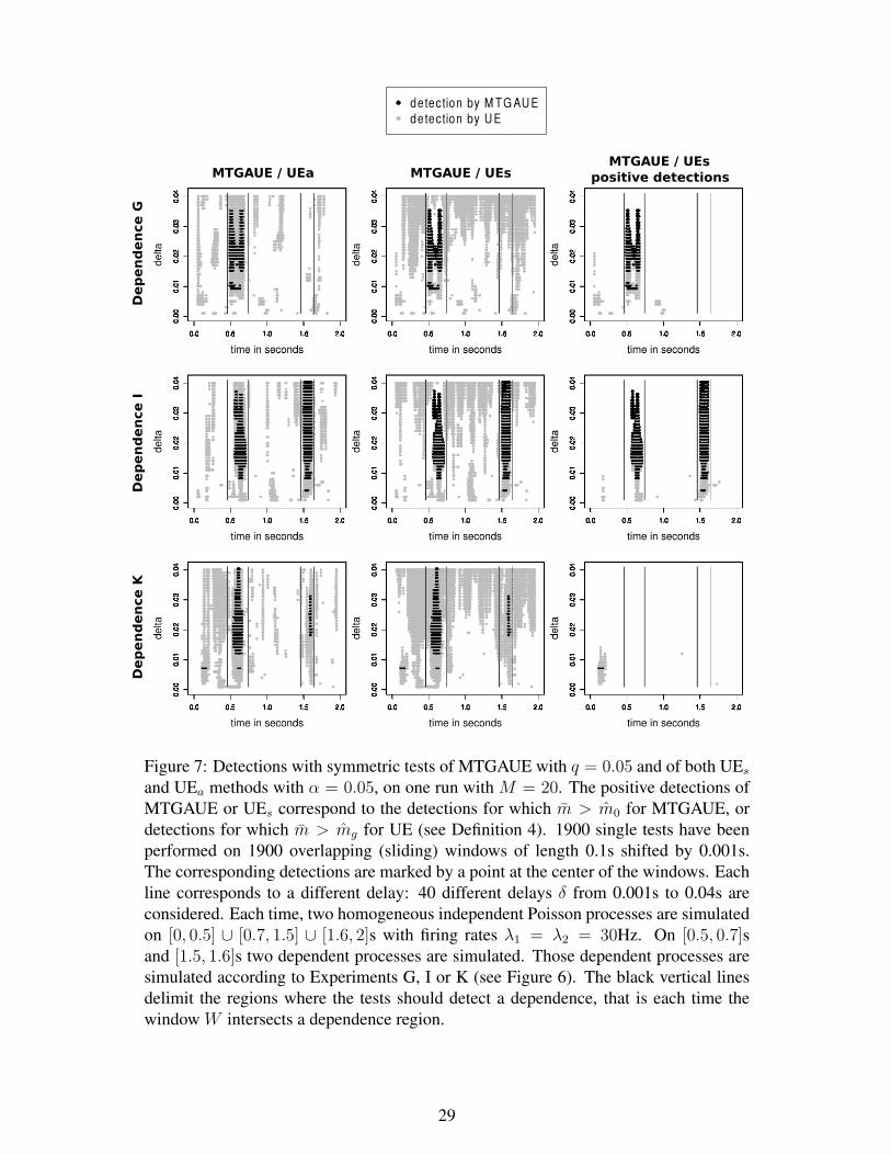
detection by M TG AU Edetection by U E
MTGAUE / UEa
Dep
en
den
ce G
Dep
en
den
ce I
Dep
en
den
ce K
MTGAUE / UEs MTGAUE / UEs
positive detections
Figure 7: Detections with symmetric tests of MTGAUE with q = 0.05 and of both UEs
and UEa methods with α = 0.05, on one run with M = 20. The positive detections of
MTGAUE or UEs correspond to the detections for which m > m0 for MTGAUE, or
detections for which m > mg for UE (see Definition 4). 1900 single tests have been
performed on 1900 overlapping (sliding) windows of length 0.1s shifted by 0.001s.
The corresponding detections are marked by a point at the center of the windows. Each
line corresponds to a different delay: 40 different delays δ from 0.001s to 0.04s are
considered. Each time, two homogeneous independent Poisson processes are simulated
on [0, 0.5] ∪ [0.7, 1.5] ∪ [1.6, 2]s with firing rates λ1 = λ2 = 30Hz. On [0.5, 0.7]sand [1.5, 1.6]s two dependent processes are simulated. Those dependent processes are
simulated according to Experiments G, I or K (see Figure 6). The black vertical lines
delimit the regions where the tests should detect a dependence, that is each time the
window W intersects a dependence region.
29
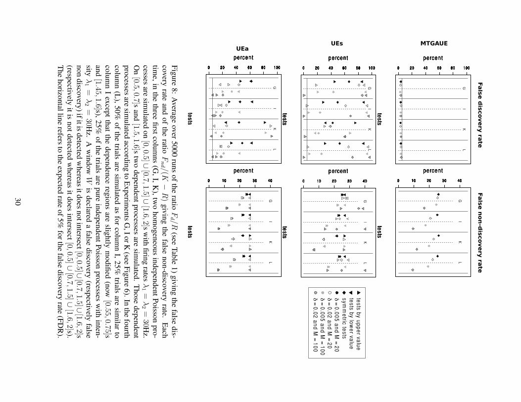
0 20 40 60 80 100
tes
ts
pe rcen t
0 20 40 60 80 100
tes
ts
pe rcen t
0 20 40 60 80 100
tes
ts
pe rcen t
0 20 40 60 80 100
tes
ts
pe rcen t
0 20 40 60 80 100
tes
ts
pe rcen t
0 20 40 60 80 1000 20 40 60 80 1000 20 40 60 80 1000 20 40 60 80 1000 20 40 60 80 1000 20 40 60 80 1000 20 40 60 80 1000 20 40 60 80 100
GI
KL
0 20 40 60 80 1000 20 40 60 80 100
tes
ts
pe rcen t
0 20 40 60 80 100
tes
ts
pe rcen t
0 20 40 60 80 100
tes
ts
pe rcen t
0 20 40 60 80 100
tes
ts
pe rcen t
0 20 40 60 80 100
tes
ts
pe rcen t
0 20 40 60 80 1000 20 40 60 80 1000 20 40 60 80 1000 20 40 60 80 1000 20 40 60 80 1000 20 40 60 80 1000 20 40 60 80 1000 20 40 60 80 1000 20 40 60 80 1000 20 40 60 80 1000 20 40 60 80 1000 20 40 60 80 1000 20 40 60 80 1000 20 40 60 80 1000 20 40 60 80 1000 20 40 60 80 100
GI
KL
0 20 40 60 80 100
0 10 20 30 40
tes
ts
pe rcen t
0 10 20 30 40
tes
ts
pe rcen t
0 10 20 30 40
tes
ts
pe rcen t
0 10 20 30 40
tes
ts
pe rcen t
0 10 20 30 40
tes
ts
pe rcen t
0 10 20 30 400 10 20 30 400 10 20 30 400 10 20 30 400 10 20 30 400 10 20 30 400 10 20 30 400 10 20 30 40
GI
KL
0 10 20 30 400 10 20 30 40
tes
ts
pe rcen t
0 10 20 30 40
tes
ts
pe rcen t
0 10 20 30 40
tes
ts
pe rcen t
0 10 20 30 40
tes
ts
pe rcen t
0 10 20 30 40
tes
ts
pe rcen t
0 10 20 30 400 10 20 30 400 10 20 30 400 10 20 30 400 10 20 30 400 10 20 30 400 10 20 30 400 10 20 30 400 10 20 30 400 10 20 30 400 10 20 30 400 10 20 30 400 10 20 30 400 10 20 30 400 10 20 30 400 10 20 30 40
GI
KL
0 10 20 30 40
tes
ts b
y u
pp
er va
lue
tes
ts b
y lo
we
r valu
es
ym
me
tric te
sts
δ=
0.0
05
an
dM=
20
δ=
0.0
2a
nd
M=
20
δ=
0.0
05
an
dM=
10
0δ=
0.0
2a
nd
M=
10
0
MTGAUEUEsUEa
Fals
e d
iscovery r
ate
Fals
e n
on
-dis
covery r
ate
Fig
ure
8:
Averag
eover
5000
runs
of
the
ratioFd /R
(seeT
able
1)
giv
ing
the
falsedis-
covery
ratean
dof
the
ratioFnd /(K
−R)
giv
ing
the
falsenon-d
iscovery
rate.E
ach
time,
inth
eth
reefi
rstco
lum
ns
(G,
I,K
),tw
ohom
ogen
eous
indep
enden
tP
oisso
npro
-
cessesare
simulated
on[0,0.5]∪
[0.7,1.5]∪[1.6,2]s
with
firin
grates
λ1=
λ2=
30H
z.
On[0.5,0.7]s
and[1.5,1.6]s
two
dep
enden
tpro
cessesare
simulated
.T
hose
dep
enden
t
pro
cessesare
simulated
accord
ing
toE
xperim
ents
G,I
or
K(see
Fig
ure
6).
Inth
efo
urth
colu
mn
(L),
50%
of
the
trialsare
simulated
asfo
rco
lum
nI,
25%
trialsare
similar
to
colu
mn
Iex
cept
that
the
dep
enden
cereg
ions
areslig
htly
modifi
ed(n
ow
[0.55,0.75]san
d[1.45,1.6]s),
25%
of
the
trialsare
pure
indep
enden
tP
oisso
npro
cessesw
ithin
ten-
sityλ1=
λ2=
30H
z.A
win
dow
Wis
declared
afalse
disco
very
(respectiv
elyfalse
non
disco
very
)if
itis
detected
whereas
itdoes
notin
tersect[0,0.5]∪[0.7,1.5]∪
[1.6,2]s(resp
ectively
itis
not
detected
whereas
itdoes
intersect
[0,0.5]∪[0.7,1.5]∪
[1.6,2]s).T
he
horizo
ntal
line
refersto
the
expected
rateof
5%
for
the
falsedisco
very
rate(F
DR
).
30
4.1 Description of the data
Behavioral procedure The data used in this theoretical article to test the detection
ability of the MTGAUE method were already partially published in previous experi-
mental studies (Riehle et al., 2000; Grammont & Riehle, 2003; Riehle et al., 2006).
These data were collected on a 5-year-old male Rhesus monkey who was trained to per-
form a delayed multidirectional pointing task. The animal sat in a primate chair in front
of a vertical panel on which seven touch-sensitive light-emitting diodes were mounted,
one in the center and six placed equidistantly (60 degrees apart) on a circle around it.
The monkey had to initiate a trial by touching and then holding with the left hand the
central target. After a fix delay of 500ms, the preparatory signal (PS) was presented by
illuminating one of the six peripheral targets in green. After a delay of either 600ms
or 1200ms, selected at random with various probability, it turned red, serving as the
response signal and pointing target. During the first part of the delay, the probability
presp for the response signal to occur at (500+600)ms =1.1s was either 0.3, 0.5 or 0.7,
depending on the experimental condition. Once this moment passed without signal oc-
currence, the conditional probability for the signal to occur at (500+600+600)ms =1.7s
changed to 1. The monkey was rewarded by a drop of juice after each correct trial. Re-
action time (RT) was defined as the release of the central target. Movement time (MT)
was defined as the touching of the correct peripheral target.
Recording technique Signals recorded from up to seven microelectrodes (quartz in-
sulated platinum-tungsten electrodes, impedance: 2-5MΩ at 1000Hz) were amplified
and band-pass filtered from 300Hz to 10kHz. Using a window discriminator, spikes
from only one single neuron per electrode were then isolated. Neuronal data along with
behavioral events (occurrences of signals and performance of the animal) were stored
on a PC for off-line analysis with a time resolution of 10kHz.
In the following study, only trials where the response signal occurs at 1.7s are consid-
ered. When presp = 0.3 (respectively 0.5 or 0.7), the corresponding data are called
Data30 (respectively Data50 and Data70). There are respectively 43, 34 and 27 pairs
of neurons that have been registered in respectively Data30, Data50 and Data70.
Assuming that the synchrony only depends on the time of signal occurrences and not
of the movement directions, we test for the independence of neuron pairs in a pooled
fashion over all direction of movement, as already done in the previous study but in
a different way (Grammont & Riehle, 2003). Note that a study with respect to the
movement directions could also have been done if data with less than 20 trials per
direction were discarded, but then Data70 would have almost completely disappeared.
Note also that small heterogeneity in the data as shown with Case L of Figure 8 does
not really affect the method. Moreover, we did not discard pairs of neurons whose firing
31
rate is smaller than 7Hz (Roy et al., 2000), as done by Riehle et al. (2000) or Grammont
& Riehle (2003) because even in this case the MTGAUE detections can be trusted (see
Figure 6).
4.2 Symmetric detections
Before making the analysis of the whole three data sets, let us focus on some examples
to underline the main difference between MTGAUE and both UE methods. MTGAUE
(see Definition 5) has been applied on the activity of two pairs of neurons (pairs 13
and 40 of Data30), recorded during the experiment described in Section 4.1, for var-
ious choices for the FDR control parameter q. Both multiple shift UE methods with
symmetric tests and with parameter α = 0.05 have also been applied. The results are
displayed in Figure 9.
The black points correspond to MTGAUE detections with q = 0.01 and conse-
quently at the most 1% of those detections are false discoveries in average. Those are
the safest detections. Because of the monotonicity in terms of q, the classical detections
with q = 0.05 correspond to the union of black and magenta points. At the opposite,
yellow circles correspond to untrusted detections since they are detected only for a FDR
control parameter q strictly larger than 80%. In this respect, on Figure 9, several periods
are detected by MTGAUE which correlate with the occurrence of specific events of the
behavorial protocol (see also Figure 12 in this respect). Interestingly, there is no real
gain by looking at the detections for q = 0.05. Most of them are already detected for
q = 0.01 for larger δ and therefore, these detections are really significant. Both UE
methods with symmetric tests and with α = 0.05 detect several intervals correspond-
ing to q > 0.8 and therefore, those are untrusted (yellow) detections for the MTGAUE
method.
4.3 Is the count significantly too low or too large ?
For single tests, the detection of ∆sym at level α = 0.05 is just the detection of both
tests ∆+ and ∆− at level α = 0.025 and this for both UE and GAUE methods (see
Definitions 3 and 4). When dealing with a collection of tests, this result is still valid for
the UE method which does not correct for multiplicity. However, it is not valid anymore
for MTGAUE (see Definition 5) since this method is based on the rank of all the p-
values of all the symmetric tests. Indeed the set of considered p-values corresponds to a
set of test statistics whose positive and negative values are mixed and whose rank only
corresponds to their absolute value. The result of Benjamini and Hochberg procedure
is consequently intertwining positive and negative detections (i.e. detections for which
m > m0 or m < m0). Since the interest lies in both distinct detections (upper and
lower values) on the experimental data, it is meaningless to independently perform tests
32
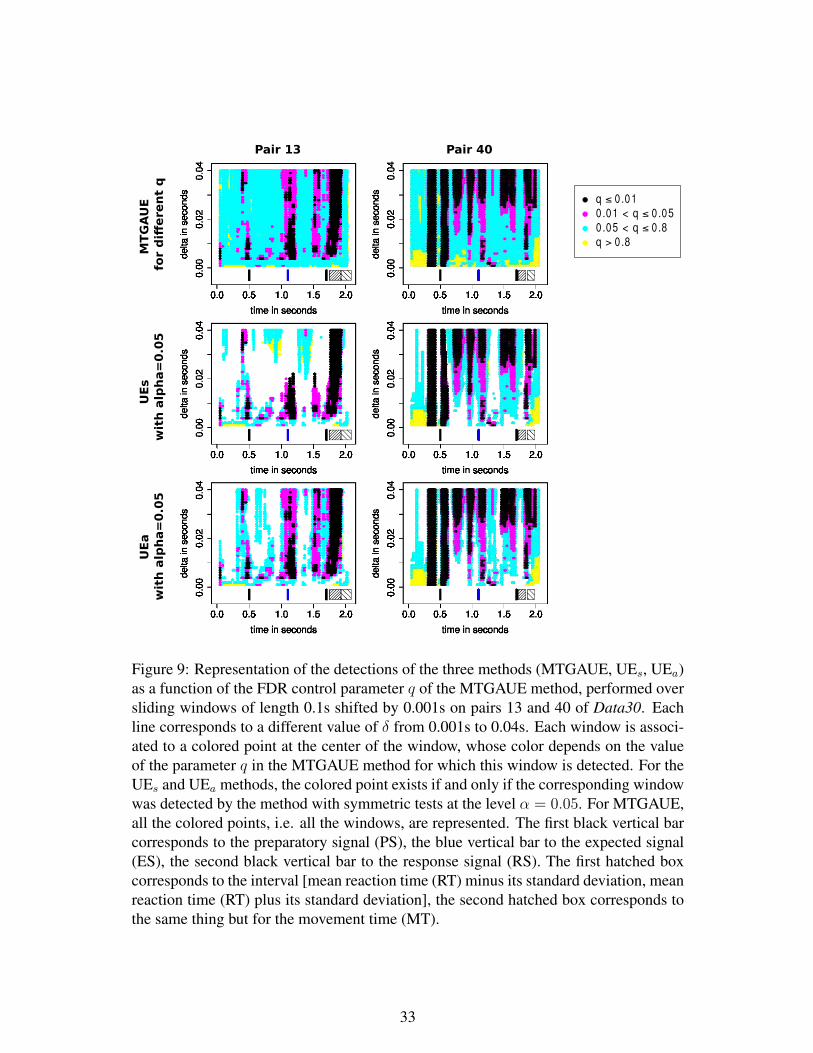
Pair 13 Pair 40 M
TG
AU
E
for d
ifferen
t q
U
Es
wit
h a
lph
a=
0.0
5
U
Ea
wit
h a
lph
a=
0.0
5
q ≤ 0.01
0.01 < q ≤ 0.05
0.05 < q ≤ 0.8
q > 0.8
Figure 9: Representation of the detections of the three methods (MTGAUE, UEs, UEa)
as a function of the FDR control parameter q of the MTGAUE method, performed over
sliding windows of length 0.1s shifted by 0.001s on pairs 13 and 40 of Data30. Each
line corresponds to a different value of δ from 0.001s to 0.04s. Each window is associ-
ated to a colored point at the center of the window, whose color depends on the value
of the parameter q in the MTGAUE method for which this window is detected. For the
UEs and UEa methods, the colored point exists if and only if the corresponding window
was detected by the method with symmetric tests at the level α = 0.05. For MTGAUE,
all the colored points, i.e. all the windows, are represented. The first black vertical bar
corresponds to the preparatory signal (PS), the blue vertical bar to the expected signal
(ES), the second black vertical bar to the response signal (RS). The first hatched box
corresponds to the interval [mean reaction time (RT) minus its standard deviation, mean
reaction time (RT) plus its standard deviation], the second hatched box corresponds to
the same thing but for the movement time (MT).
33

Pair 13 Pair 40
MTG
AU
EU
Es
negative detection
positive de tection
Figure 10: Detections according to the sign of the test statistics for MTGAUE and UEs
(symmetric count). Both methods have been run on pairs 13 and 40 with δ = 0.02s and
q = α = 0.05 over sliding windows of length 0.1s shifted by 0.001s with symmetric
tests. Lines correspond to trials, first bottom half corresponding to N1 and second upper
half to N2. Points correspond to spikes: by default their color is grey. Couples of points
(x, y) with delay less than δ are then colored in red if they belong to a window, which is
a positive detection by the considered method, i.e. m > m0 (for MTGAUE) or m > mg
(for UEs). They are colored in blue if they belong to a window, which is a negative
detection by the considered method, i.e. m < m0 (for MTGAUE) or m < mg (for
UEs).
by upper values and then tests by lower values. The correct way to use the method is
consequently to perform MTGAUE with the symmetric tests, as defined in Definition
5. Once a window is detected, one can then ask the question whether this detection was
due to a low count or a large count by looking at the sign of m− m0, which is coherent
with Figure 7.
Figures 10 and 11 show the detections according to their signs. On Figure 10, the
UEs positive detections are more or less included in the ones of MTGAUE and the
detections that are done by UEs and not MTGAUE are mostly negative detections, both
facts being coherent with Figure 7. On Figure 11, UEa detects more coincidence than
MTGAUE, fact which is also coherent with Figure 7. More importantly, we see here on
real data, that exchanging the role of N1 and N2 can drastically change the conclusion:
whole regions are detected or not depending on which spike train is restricted to the
34
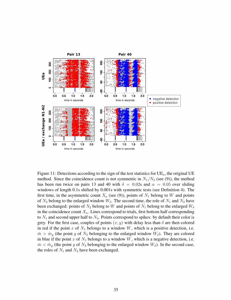
Pair 13 Pair 40
UEa
UEa /
exch
an
ge N
1-N
2
negative de tection
positive de tection
Figure 11: Detections according to the sign of the test statistics for UEa, the original UE
method. Since the coincidence count is not symmetric in N1/N2 (see (9)), the method
has been run twice on pairs 13 and 40 with δ = 0.02s and α = 0.05 over sliding
windows of length 0.1s shifted by 0.001s with symmetric tests (see Definition 4). The
first time, in the asymmetric count Xa (see (9)), points of N1 belong to W and points
of N2 belong to the enlarged window Wδ. The second time, the role of N1 and N2 have
been exchanged: points of N2 belong to W and points of N1 belong to the enlarged Wδ
in the coincidence count Xa. Lines correspond to trials, first bottom half corresponding
to N1 and second upper half to N2. Points correspond to spikes: by default their color is
grey. For the first case, couples of points (x, y) with delay less than δ are then colored
in red if the point x of N1 belongs to a window W , which is a positive detection, i.e.
m > mg (the point y of N2 belonging to the enlarged window Wδ). They are colored
in blue if the point x of N1 belongs to a window W , which is a negative detection, i.e.
m < mg (the point y of N2 belonging to the enlarged window Wδ). In the second case,
the roles of N1 and N2 have been exchanged.
35
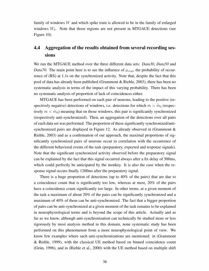
family of windows W and which spike train is allowed to be in the family of enlarged
windows Wδ. Note that those regions are not present in MTGAUE detections (see
Figure 10).
4.4 Aggregation of the results obtained from several recording ses-
sions
We run the MTGAUE method over the three different data sets: Data30, Data50 and
Data70. The main point here is to see the influence of presp, the probability of occur-
rence of (RS) at 1.1s on the synchronized activity. Note that, despite the fact that this
pool of data has already been published (Grammont & Riehle, 2003), there has been no
systematic analysis in terms of the impact of this varying probability. There has been
no systematic analysis of proportion of lack of coincidences either.
MTGAUE has been performed on each pair of neurons, leading to the positive (re-
spectively negative) detections of windows, i.e. detections for which m > m0 (respec-
tively m < m0) meaning that on those windows, this pair is significantly synchronized
(respectively anti-synchronized). Then, an aggregation of the detections over all pairs
of each data set was performed. The proportion of these significantly synchronized/anti-
synchronized pairs are displayed in Figure 12. As already observed in (Grammont &
Riehle, 2003) and as a confirmation of our approach, the maximal proportions of sig-
nificantly synchronized pairs of neurons occur in correlation with the occurrence of
the different behavioral events of the task (preparatory, expected and response signals).
Note that the significant synchronized activity observed before the preparatory signal
can be explained by the fact that this signal occurred always after a fix delay of 500ms,
which could perfectly be anticipated by the monkey. It is also the case when the re-
sponse signal occurs finally 1200ms after the preparatory signal.
There is a huge proportion of detections (up to 40% of the pairs) that are due to
a coincidence count that is significantly too low, whereas at most, 20% of the pairs
have a coincidence count significantly too large. In other terms, at a given moment of
the task a maximum of about 20% of the pairs can be significantly synchronized and a
maximum of 40% of them can be anti-synchronized. The fact that a bigger proportion
of pairs can be anti-synchronized at a given moment of the task remains to be explained
in neurophysiological terms and is beyond the scope of this article. Actually and as
far as we know, although anti-synchronization can technically be studied more or less
rigorously by most analysis method in this domain, none systematic study has been
performed on this phenomenon from a more neurophysiological point of view. We
know few examples where such anti-synchronizations are mentioned: in (Grammont
& Riehle, 1999), with the classical UE method based on binned coincidence count
(Grun, 1996), and in (Riehle et al., 2000) with the UE method based on multiple shift
36
0 0.025 0.05 0.084 0.11 0.21 0 0.08 0.16 0.22 0.36 0.42
Positive detections Negative detections
Data30
Data50
Data70
Scale of proportions
Figure 12: Proportion of positive detections/negative detections, i.e. of significantly
synchronized/anti-synchronized pairs of neurons using MTGAUE method (sliding win-
dows of length 0.1s shifted by 0.001s, q = 0.05) through time. Each line represents a
different parameter δ ∈ 1, ..., 40 × 10−3s. (PS) was presented at 0.5s (first vertical
black line), (RS) at 1.7s (third vertical black line). Even if those trials are not used in
the present average, a response signal at 1.1s ((ES)=second vertical black line) was also
presented to the animal in 30% of the cases for Data30, in 50% of the cases for Data50
and in 70% of the cases for Data70.
37

coincidence count (Grun et al., 1999).
• Significantly too large coincidence count.
The proportion of significantly synchronized pairs in Figure 12 is much more
important on Data30, showing two maxima, just after the expected signal (ES)
and just after the response signal (RS). When the probability of (ES) increases
(Data50 and Data70), those maxima still appear but in a lower proportion. There-
fore it appears with this new analysis that the proportion of synchronized pairs
tends to diminish when the probability of (RS) at 1.1s increases. Moreover, when
the response signal at 1.1s is much more likely than the response signal at 1.7s (in
Data70), those maxima are shifted in time as if the animal continued to expect
the signal for a longer time.
• Significantly too low coincidence count.
In Figure 12, it appears that all the three data sets have roughly the same maximal
proportion of pairs that are significantly anti-synchronized. The main difference
comes from the localization and the fuzziness of the proportion of pairs. The
maxima are large and strong in Data30 in particular around the preparatory and
expected signals. In Data70, the only localizations reaching such high scores are
just before and after (ES). In Data50, the signal is fuzzier and it is harder to give
a rigorous interpretation.
5 Discussion
We presented a generalization, namely the delayed coincidence count, of the notion
of multiple shift coincidence count (Grun et al., 1999) to point processes that are not
discretized at a given resolution.
The multiple shift notion is already known to clearly outperform classical binned
coincidence count, since there is, in particular, no loss in synchrony detection due to
binning effects as already pointed out in (Grun et al., 1999). However, this notion is
not as popular as the binned coincidence count mainly because its statistical properties
were much more opaque, until the present work. Actually, the multiple shift coinci-
dence count can be interpreted in two ways: symmetric and asymmetric (see Figure
1). But when testing a symmetric hypothesis, namely the independence of both spike
trains, the use of an asymmetric notion, which is the original version that has been
programmed in the UE method, leads to answers that depend on which spike train is
referred as N1 (see Figure 11 for an example on real data). Therefore we focused in
this article on the symmetric notion of multiple shift coincidence count to prevent this
effect. The delayed coincidence count, introduced in this article, is the generalization
38
of the symmetric multiple shift coincidence count to the non discretized point process
framework. This notion allows us to perform complete computations when Poisson
processes are involved. It consequently also reveals some basic properties of the (sym-
metric) multiple shift coincidence count for Bernoulli processes, this model being very
well approximated by Poisson processes as proved in Section 2.3.
The first novel property is that the multiple shift coincidence count (symmetric or
not), as well as the delayed coincidence count, is not Poisson distributed, but more dis-
persed, when both spike trains are independent homogeneous Poisson processes. The
Fano factor computed in (16) for the delayed coincidence count and Poisson processes,
is strictly larger than 1 and this gap tends to increase with the firing rate and the delay
δ. In (Grun et al., 1999), the distribution of the (asymmetric) multiple shift coincidence
count is approximated by a Poisson distribution with mean mg (see (6) or (10)). How-
ever Figures 3 and 4 show that neither the symmetric nor the asymmetric multiple shift
coincidence count is Poisson, whereas the Gaussian approximation that has been de-
rived in Theorem 1, correctly approximates the symmetric multiple shift coincidence
count, when Poisson or Bernoulli processes are involved. Moreover, when considering
symmetric multiple shift coincidence count, there is an edge effect in the mean (m0
and not mg, see (12)) that needs to be taken into account (see again Figure 3 and also
Theorem 1). For asymmetric multiple shift coincidence count, the mean is correctly
predicted by mg but not the variance.
Those properties would be useless, if they could not be turned into a real statistical
test. To do so, we investigated the plug-in step, showing that a modification of the
variance need to be taken into account (see Theorem 2). Our GAUE (for Gaussian
approximation of the Unitary Events) tests (see also Definition 3) are therefore proved
to be of asymptotical level α, when homogeneous Poisson processes are considered as
models of the spike trains. They are also proved to be robust on simulations where small
firing rates, non stationarity or refractory periods have been imposed and this even for
the test by lower value, which is able to detect lack of coincidences (see Figure 6). We
also see that for large enough firing rate λ (λ = 30Hz), the three original UEa tests of
(Grun et al., 1999), based on the asymmetric count (see also Definition 4) have type
I error α = 5%. This is in the range of parameters where the original UE method
with the multiple shift coincidence count, based on a Poissonian approximation, can
be used. For very small firing rates, the type I errors of all UE tests (with symmetric
or asymmetric count) are huge, fact which is consistent with (Roy et al., 2000) (see
Figure 6, Experiments A). For large δ and large firing rates, the UEs test by upper
values (with symmetric count) becomes too conservative (see Figure 6, Experiments
B). On the contrary, both UEs tests (symmetric or by lower values) have very large type
I error (more than 20%), and this can even increase with the number of trials M . This
is coherent with Figure 5, where we clearly see that the Poisson approximation of the
39

asymmetric count is quite accurate but that the Poisson approximation of the symmetric
count is not correctly centred, making the UEs test by upper values more conservative
but the other UEs tests (symmetric and by lower values) untrustworthy. In this sense,
even if UEs tests (symmetric or by lower values) have larger power than GAUE tests
for detecting lack of coincidences (see Figure 6, Experiments J and K), they cannot be
preferred to the GAUE tests since there is no control of their type I error. Finally note
that all UEa methods and UEs method by upper values have level α = 0.05 when non
stationary processes or refractory periods with small δ are tested (Experiments C, D and
E). But both UEs tests (symmetric and by lower values) with large δ have a type I error
which clearly becomes huge when M , the number of trials, grows and when refractory
periods are present (Experiments D and E).
Two other methods in the literature do not need plug-in steps. On the one hand, con-
ditional probability computations can be performed on binned coincidence count (Gutig
et al., 2001), but it will be, in our opinion very difficult to transfer those computations to
the delayed coincidence count, since the use of independent Bernoulli variables is fun-
damental. On the other hand, trial-shuffling methods (Pipa et al., 2003; Pipa & Grun,
2003) have also been used for binned coincidence count. This kind of resampling meth-
ods could be mathematically adapted to the delayed coincidence count and could furnish
a prescribed type I error control of the resulting test. However, the combinatorics of the
delayed coincidence count is much more complex than the binned coincidence count.
Therefore, a first step in this direction would be to develop a fast algorithm of delayed
coincidence count. As a second step, classical parallel programming could make the
trial-shuffling procedure combined with delayed coincidence count effective in practice
(Denker et al., 2010). More generally, many other surrogate data methods exist (see
(Louis et al., 2010) for dithering or (Grun, 2009) for a more general review). In our
opinion, it would be decisive, as a future work, to find a procedure which combines an
effective surrogate data method of this kind with a prescribed type I error control.
The final step of our procedure is the use of Benjamini and Hochberg’s method to
control the false discovery rate (FDR) by the choice of a parameter q (Benjamini &
Hochberg, 1995). Our method, MTGAUE, is proved on various simulations to guar-
antee the correct FDR (see Figure 8). On the contrary, the classical UE method is
not corrected for multiplicity. Simulations show that this choice leads to a huge FDR,
sometimes as high as 80%. Only for the UEs method with tests by upper values for
large delays δ (δ = 0.02s) and only for the UEa method with tests by lower values for
very large M (M = 100) and large δ (δ = 0.02s), is the UE method trustworthy. This is
coherent with the visualisation of both methods on just one run (see Figure 7). Clearly
for large δ the number of false discoveries by the symmetric UE method (UEs or UEa)
is huge whereas the detections by upper values of UEs are globally adequate, with a
tendency to be less accurate for small δ. This phenomenon can be explained as follows.
40
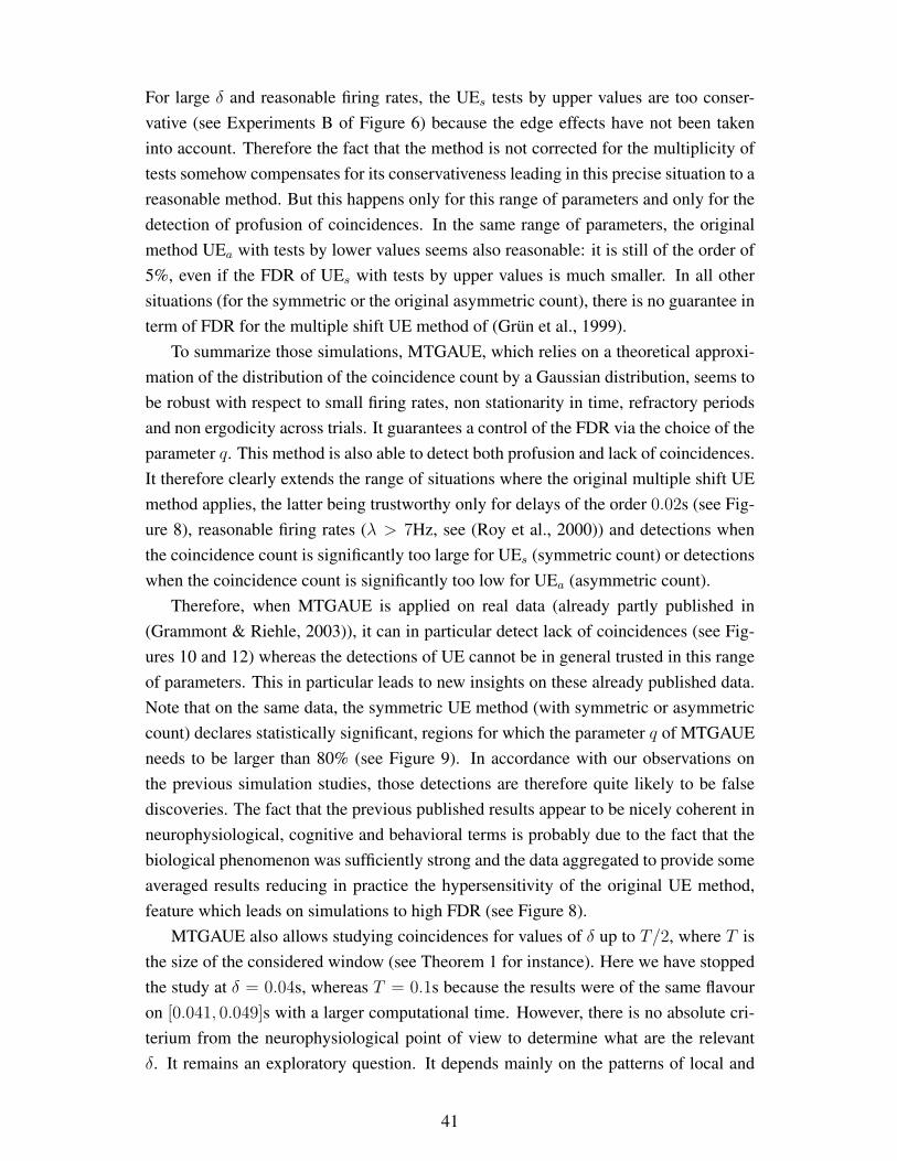
For large δ and reasonable firing rates, the UEs tests by upper values are too conser-
vative (see Experiments B of Figure 6) because the edge effects have not been taken
into account. Therefore the fact that the method is not corrected for the multiplicity of
tests somehow compensates for its conservativeness leading in this precise situation to a
reasonable method. But this happens only for this range of parameters and only for the
detection of profusion of coincidences. In the same range of parameters, the original
method UEa with tests by lower values seems also reasonable: it is still of the order of
5%, even if the FDR of UEs with tests by upper values is much smaller. In all other
situations (for the symmetric or the original asymmetric count), there is no guarantee in
term of FDR for the multiple shift UE method of (Grun et al., 1999).
To summarize those simulations, MTGAUE, which relies on a theoretical approxi-
mation of the distribution of the coincidence count by a Gaussian distribution, seems to
be robust with respect to small firing rates, non stationarity in time, refractory periods
and non ergodicity across trials. It guarantees a control of the FDR via the choice of the
parameter q. This method is also able to detect both profusion and lack of coincidences.
It therefore clearly extends the range of situations where the original multiple shift UE
method applies, the latter being trustworthy only for delays of the order 0.02s (see Fig-
ure 8), reasonable firing rates (λ > 7Hz, see (Roy et al., 2000)) and detections when
the coincidence count is significantly too large for UEs (symmetric count) or detections
when the coincidence count is significantly too low for UEa (asymmetric count).
Therefore, when MTGAUE is applied on real data (already partly published in
(Grammont & Riehle, 2003)), it can in particular detect lack of coincidences (see Fig-
ures 10 and 12) whereas the detections of UE cannot be in general trusted in this range
of parameters. This in particular leads to new insights on these already published data.
Note that on the same data, the symmetric UE method (with symmetric or asymmetric
count) declares statistically significant, regions for which the parameter q of MTGAUE
needs to be larger than 80% (see Figure 9). In accordance with our observations on
the previous simulation studies, those detections are therefore quite likely to be false
discoveries. The fact that the previous published results appear to be nicely coherent in
neurophysiological, cognitive and behavioral terms is probably due to the fact that the
biological phenomenon was sufficiently strong and the data aggregated to provide some
averaged results reducing in practice the hypersensitivity of the original UE method,
feature which leads on simulations to high FDR (see Figure 8).
MTGAUE also allows studying coincidences for values of δ up to T/2, where T is
the size of the considered window (see Theorem 1 for instance). Here we have stopped
the study at δ = 0.04s, whereas T = 0.1s because the results were of the same flavour
on [0.041, 0.049]s with a larger computational time. However, there is no absolute cri-
terium from the neurophysiological point of view to determine what are the relevant
δ. It remains an exploratory question. It depends mainly on the patterns of local and
41
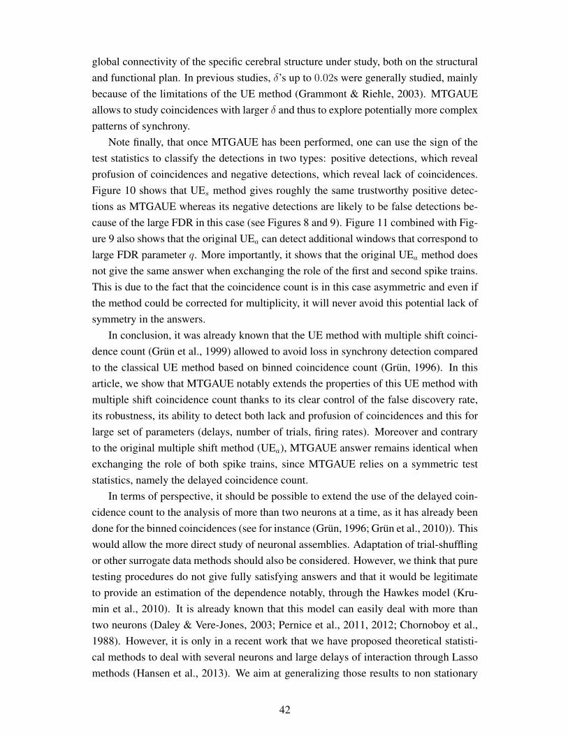
global connectivity of the specific cerebral structure under study, both on the structural
and functional plan. In previous studies, δ’s up to 0.02s were generally studied, mainly
because of the limitations of the UE method (Grammont & Riehle, 2003). MTGAUE
allows to study coincidences with larger δ and thus to explore potentially more complex
patterns of synchrony.
Note finally, that once MTGAUE has been performed, one can use the sign of the
test statistics to classify the detections in two types: positive detections, which reveal
profusion of coincidences and negative detections, which reveal lack of coincidences.
Figure 10 shows that UEs method gives roughly the same trustworthy positive detec-
tions as MTGAUE whereas its negative detections are likely to be false detections be-
cause of the large FDR in this case (see Figures 8 and 9). Figure 11 combined with Fig-
ure 9 also shows that the original UEa can detect additional windows that correspond to
large FDR parameter q. More importantly, it shows that the original UEa method does
not give the same answer when exchanging the role of the first and second spike trains.
This is due to the fact that the coincidence count is in this case asymmetric and even if
the method could be corrected for multiplicity, it will never avoid this potential lack of
symmetry in the answers.
In conclusion, it was already known that the UE method with multiple shift coinci-
dence count (Grun et al., 1999) allowed to avoid loss in synchrony detection compared
to the classical UE method based on binned coincidence count (Grun, 1996). In this
article, we show that MTGAUE notably extends the properties of this UE method with
multiple shift coincidence count thanks to its clear control of the false discovery rate,
its robustness, its ability to detect both lack and profusion of coincidences and this for
large set of parameters (delays, number of trials, firing rates). Moreover and contrary
to the original multiple shift method (UEa), MTGAUE answer remains identical when
exchanging the role of both spike trains, since MTGAUE relies on a symmetric test
statistics, namely the delayed coincidence count.
In terms of perspective, it should be possible to extend the use of the delayed coin-
cidence count to the analysis of more than two neurons at a time, as it has already been
done for the binned coincidences (see for instance (Grun, 1996; Grun et al., 2010)). This
would allow the more direct study of neuronal assemblies. Adaptation of trial-shuffling
or other surrogate data methods should also be considered. However, we think that pure
testing procedures do not give fully satisfying answers and that it would be legitimate
to provide an estimation of the dependence notably, through the Hawkes model (Kru-
min et al., 2010). It is already known that this model can easily deal with more than
two neurons (Daley & Vere-Jones, 2003; Pernice et al., 2011, 2012; Chornoboy et al.,
1988). However, it is only in a recent work that we have proposed theoretical statisti-
cal methods to deal with several neurons and large delays of interaction through Lasso
methods (Hansen et al., 2013). We aim at generalizing those results to non stationary
42

data in time.
Acknowledgments
We first of all want to thank Alexa Riehle, leader of the laboratory in which the data
used in this article were previously collected. We wish also to thank Y. Bouret and
F. Picard for fruitful discussions and programming help at several stages of this work.
Finally, we thank two anonymous referees for their thorough work on our manuscript
and their helpful comments. This research is partly supported by the french Agence
Nationale de la Recherche (ANR 2011 BS01 010 01 projet Calibration), by the PEPS
BMI 2012-2013 Estimation of dependence graphs for thalamo-cortical neurons and
multivariate Hawkes processes and the PEPS BMI 2012-2013 NeuroConf.
The authors want to precise that CTM is the main contributor to the applied method,
its simulation and the treatment of the real data sets ; PRB is at the origin of the theo-
retical method, contributed to the applied study and did most of the redaction ; AR is
a predoctoral student who ran most of the preliminary study during her internship ; FG
initiated the project by introducing CTM, PRB and AR to the neuroscientific issues and
to the informal notion of coincidence, he also gave insight on the real data sets that he
recorded in Alexa Riehle’s Laboratory.
References
Abeles, M. (1982). Quantification, smoothing, and confidence-limits for single-units
histograms. Journal of Neuroscience Methods, 5(4), 317–325.
Abeles, M. (1991). Corticonics. Neural circuits in the cerebral cortex. Cambridge
University Press.
Abeles, M., & Gat, I. (2001). Detecting precise firing sequences in experimental data.
Journal of Neuroscience Methods, 107, 141–154.
Aertsen, A.M., Gerstein, G.L., Habib, M.K., & Palm, G. (1989). Dynamics of neuronal
firing correlation: modulation of ”effective connectivity”. Journal of Neurophysiol-
ogy, 61(5), 900–917.
Benjamini, Y. (2010). Discovering the false discovery rate. Journal of the Royal Statis-
tical Society, Series B, 72(4), 405–416.
Benjamini, Y. & Hochberg, Y., (1995). Controlling the false discovery rate: a practical
and powerful approach to multiple testing. Journal of the Royal Statistical Society,
Series B, 57(1), 289–300.
43
Benjamini, Y. & Yekutieli, D., (2001). The control of the false discovery rate in multiple
testing under dependency. Annals of Statistics, 29(4), 1165–1188.
Boucsein, C., Nawrot, M.P., Schnepel, P., & Aertsen, A.M. (2011). Beyond the cortical
column: abundance and physiology of horizontal connections imply a strong role for
inputs from the surround. Frontiers in Neuroscience, (5), article 32.
Brette, R. (2012). Computing with neural synchrony. PLoS Computational Biology,
8(6), e1002561.
Brown, E., Barbieri, R., Ventura, V., Kass, R., & Frank, L. (2002). The time rescaling
theorem and its application to neural spike train analysis. Neural Computation, 14(2),
325–346.
Chornoboy, E.S., Schramm, L.P., & Karr, A.F. (1988). Maximum likelihood identifica-
tion of neural point process systems., Biological Cybernetics, 59, 265–275.
Denker, M., Wiebelt, B., Fliegner, D., Diesmann, M., & Morrison, A. (2010). Prac-
tically Trivial Parallel Data Processing in a Neuroscience Laboratory. In Analysis
of Parallel Spike Trains, Grun, S., & Rotter, S., Springer Series in Computational
Neuroscience.
Daley, D.J., & Vere-Jones, D. (2003). An introduction to the theory of point processes,
vol. I. Springer.
Diesmann, M., Gewaltig, M.O., & Aertsen, A.M. (1999). Stable propagation of syn-
chronous spiking in cortical neural networks. Nature, 402, 529–533.
Engel, A.K., & Singer, W. (2001). Temporal binding and the neural correlates of sen-
sory awareness. TRENDS in Cognitive Sciences, 5(1), 16–25.
Eyherabide, H.G., Rokem, A., Herz, A.V.M., & Samengo, I. (2009). Bursts generate a
non-reducible spike-pattern code. Frontiers in Neuroscience, 3(1), 8–14.
Gerstein, G.L. (2004). Searching for significance in spatio-temporal firing patterns.
Acta Neurobiologia Experimentalis, 64, 203–207.
Gerstein, G.L., & Aertsen, A.M. (1985). Representation of cooperative firing activity
among simultaneously recorded neurons. Journal of Neurophysiology, 54(6), 1513–
1528.
Gerstein, G.L., & Perkel, D.H. (1969). Simultaneous recorded trains of action poten-
tials: analysis and functional interpretation. Science, 164, 828–830.
44
Goedeke, S., & Diesmann, M. (2008). The mechanism of synchronization in feed-
forward neuronal networks. New Journal of Physics, 10, 015007.
Golomb, D., & Hansel, D. (2000). The number of synaptic inputs and the synchrony of
large sparse neuronal networks. Neural Computation, 12(5), 1095–1139.
Grammont, F., & Riehle, A. (1999). Precise spike synchronization in monkey motor
cortex involved in preparation for movement. Experimental Brain Research, 128(1-
2), 118–122.
Grammont, F., & Riehle, A. (2003). Spike synchronisation and firing rate in a popula-
tion of motor cortical neurons in relation to movement direction and reaction time.
Biological Cybernetics, 88, 360–373.
Grun, S. (1996). Unitary joint-events in multiple-neuron spiking activity: Detection,
significance and interpretation. Thun: Verlag Harri Deutsch.
Grun, S. (2009). Data-driven significance estimation for precise spike correlation. Jour-
nal of Neurophysiology, 101, 1126–1140.
Grun, S., Diesman, M., & Aertsen, A.M. (2002a). Unitary events in multiple single-
neuron spiking activity: I. Detection and Significance. Neural Computation, 14,
43–80.
Grun, S., Diesman, M., & Aertsen, A.M. (2002b). Unitary events in multiple single-
neuron spiking activity: II. Nonstationary Data. Neural Computation, 14, 81–119.
Grun, S., Diesmann, M., & Aertsen, A.M. (2010). Unitary Events Analysis. In Analysis
of Parallel Spike Trains, Grun, S., & Rotter, S., Springer Series in Computational
Neuroscience.
Grun, S., Diesmann, M., Grammont, F., Riehle, A., & Aertsen, A.M. (1999). Detecting
unitary events without discretization of time. Journal of Neuroscience Methods, 93,
67–79.
Grun, S., Riehle, A., & Diesmann, M. (1999). Effect of cross-trial nonstationarity on
joint-spike events. Biological Cybernetics, 88, 335–351.
Gutig, R., Aertsen, A.M., & Rotter, S. (2001). Statistical Significance of Coincident
Spikes: Count-Based Versus Rate-Based Statistics. Neural Computation, 14, 121–
153.
Hansen, N.R., Reynaud-Bouret, P., & Rivoirard, V. (2013). Lasso and probabilistic in-
equalities for multivariate point processes. http://arxiv.org/abs/1208.0570, to appear
in Bernoulli.
45
Hebb, D. O. (1949). Organization of behavior; a neuropsychological theory. New
York: John Wiley & Sons.
Heinzle, J., Konig, P., & Salazar R.F. (2007). Modulation of synchrony without changes
in firing rate. Cognitive Neurodynamics, 1, 225–235.
Hochberg, Y., & Tamhame, A. (1987). Multiple comparison procedures. New York:
Wiley.
Hogg, R.V., & Tanis, E.A. (2009). Probability and statistical inference. Pearson.
Holm, S. (1979). A simple sequentially rejection multiple test procedure. Scandinavian
Journal of Statistics, 6(2), 65–70.
Kilavik, B.E., Roux, S., Ponce-Alvarez, A. Confais, J. Grun, S. & Riehle, A. (2009).
Long-term modifications in motor cortical dynamics induced by intensive practice.
Journal of Neuroscience, 29(40), 12653–12663.
Konig, P., Engel, A.K., & Singer, W. (1996). Integrator or coincidence detector? The
role of the cortical neuron revisited. Trends in Neurosciences, 19(4), 130–137.
Konishi, M., Takahashi, T.T., Wagner, H., Sullivan, W.E., & Carr, C.E. (1988). Neuro-
physiological and anatomical substrates of sound localization in the owl. In Auditory
Function, Edelman, G.M., Gall, W.E. and Cowan, W.M., Wiley, New-York.
Krumin, M., Reutsky, I., & Shoham, S. (2010). Correlation-based analysis and genera-
tion of multiple spike trains using Hawkes models with an exogenous input. Frontiers
in Computational Neuroscience, 4, article 147.
Kumar, A., Rotter, S., & Aertsen, A.M. (2010). Spiking activity propagation in neu-
ronal networks: reconciling different perspectives on neural coding. Nature Reviews
Neuroscience, 11, 615–627.
Lestienne, R. (1996). Determination of the precision of spike timing in the visual cortex
of anaesthetised cats. Biological Cybernetics, 74, 55–61.
Lestienne, R. (2001). Spike timing, synchronization and information processing on the
sensory side of the central nervous system. Progress in Neurobiology, 65, 545–591.
Louis, S., Borgelt, C., & Grun, S. (2010). Generation and Selection of Surrogate Meth-
ods for Correlation Analysis. In Analysis of Parallel Spike Trains, Grun, S., & Rotter,
S., Springer Series in Computational Neuroscience.
Louis, S., Gerstein, G.L., Grun, S., & Diesmann, M. (2010). Surrogate spike train
generation through dithering in operational time. Frontiers in Computational Neuro-
science, 4(127), doi:10.3389/fncom.2010.00127
46
Mainen, Z.F., & Sejnowski, T.J. (1995). Reliability of spike timing in neocortical neu-
rons. Science, 268, 1503–1506.
Maimon, G., & Assad, J.A. (2009). Beyond Poisson: increased spike-time regularity
across primate parietal cortex. Neuron, 62(3), 426–440.
Maldonado, P.E., Babul, C., Singer, W., Rodriguez, E., Berger, D., & Grun, S. (2008).
Synchronization of neuronal response in primary visual cortex of monkeys viewing
natural images. Journal of Neurophysiology, 100, 1523–1532.
Maldonado, P.E., Friedman-Hill, S., & Gray, C.M. (2000). Dynamics of striate cortical
activity in the alert macaque: II. Fast time scale synchronization. Cerebral Cortex,
10, 1117–1131.
Masuda, N., & Aihara, K. (2007). Dual coding hypotheses for neural information rep-
resentation. Mathematical Biosciences, 207, 312–321.
Ogata, Y. (1981). On Lewis Simulation Method for Point Processes. Journal of the
American Statistical Association, 83(401), 9–27.
Ogata, Y. (1988). Statistical models for earthquakes occurrences and residual analysis
for point processes. IEEE Transactions on Information Theory, 27(1), 23–31.
Palm, G. (1990). Cell assemblies as a guideline for brain research. Concepts in Neuro-
science, 1, 133–148.
Pazienti, A., Maldonado, P.E., Diesmann, M., & Grun, S. (2008). Effectiveness of sys-
tematic spike dithering depends on the precision of cortical synchronization. Brain
Research, 1225, 39–46.
Perkel, D.H., Gernstein, G.L., & Moore, G.P. (1967). Neuronal spike trains and stochas-
tic point processes. Biophysical Journal, 7, 419–440.
Pernice, V., Staude, B., Cardanobile, S., & Rotter, S. (2011). How structure determines
correlations in neuronal networks. PLoS Computational Biology, 7, e1002059.
Pernice, V., Staude, B., Cardanobile, S., & Rotter, S. Recurrent interactions in spiking
networks with arbitrary topology. Physical review E, Statistical, nonlinear, and soft
matter physics, 85, 031916.
Pipa, G., Diesmann, M., & Grun, S. (2003). Significance of joint-spike events based on
trial-shuffling by efficient combinatorial methods. Complexity, 8(4), 1–8.
Pipa, G., & Grun, S. (2003). Non-parametric significance estimation of joint-spike
events by shuffling and resampling. Neurocomputing, 52-54, 31–37.
47
Pipa, G., Grun, S., & van Vreeswijk, C. (2013). Impact of Spike Train Autostructure on
Probability Distribution of Joint Spike Events. Neural Computation, 25, 1123–1163.
Prescott, S.A., Ratte, S., De Koninck, Y., & Sejnowski, T.J. (2008). Pyramidal neurons
switch from integrators in vitro to resonators under in vivo-like conditions. Journal
of Neurophysiology, 100, 3030–3042.
Reimer, I.C.G., Staude, B., Ehm, W., & Rotter, S. (2012). Modeling and analyzing
higher-order correlations in non-Poissonian spike trains. Journal of Neuroscience
Methods, 208, 18–33.
Reynaud-Bouret, P., Tuleau-Malot, C., Rivoirard, V., & Grammont, F. (2013). Spike
trains as (in)homogeneous Poisson processes or Hawkes processes: non-parametric
adaptive estimation and goodness-of-fit tests. http://hal.archives-ouvertes.fr/hal-
00789127, submitted.
Riehle, A., Grammont, F., Diesmann, M. & Grun, S. (2000). Dynamical changes and
temporal precision of synchronised spiking activity in monkey motor cortex during
movement preparation. Journal of Physiology, 94, 569–582.
Riehle, A., Grammont, F., & MacKay, A. (2006). Cancellation of a planned movement
in monkey motor cortex. Neuroreport, 17(3), 281–285.
Riehle, A., Grun, S., Diesmann, M., & Aertsen, A.M. (1997). Spike synchronization
and rate modulation differentially involved in motor cortical function. Science, 278,
1950–1953.
Roy, A., Steinmetz, P.N., & Niebur, E. (2000). Rate Limitations of Unitary Event
Analysis. Neural Computation, 12(9), 2063–2082.
Rudolph, M., & Destexhe, A. (2003). Tuning neocortical pyramidal neurons between
integrators and coincidence detectors. Journal of Computational Neuroscience, 14,
239–251.
Sakurai, Y. (1999). How do cell assemblies encode information in the brain? Neuro-
science and Biobehavioral Reviews, 23, 785–796.
Shinomoto, S. (2010). Estimating the Firing Rate. In Analysis of Parallel Spike Trains,
Grun, S., & Rotter, S., Springer Series in Computational Neuroscience.
Singer, W. (1993). Synchronization of cortical activity and its putative role in informa-
tion processing and learning. Annual Review of Physiology, 55, 349–374.
Singer, W. (1999). Neuronal synchrony: a versatile code for the definition of relations?
Neuron, 24, 49–65.
48
Singer, W., & Gray, C.M. (1995). Visual feature integration and the temporal correlation
hypothesis. Annual Review of Neuroscience, 18, 555–586.
Softky, W.R., & Koch, C. (1993). The highly irregular firing of cortical cells is incon-
sistent with temporal integration of random EPSPs. Journal of Neuroscience, 13(1),
334–350.
Staude, B., Rotter, S., & Grun, S. (2010). CuBIC: cumulant based inference of higher-
order correlations in massively parallel spike trains. Journal of Computational Neu-
roscience, 29, 327–350.
Super, H., van der Togt, C., Spekreijse, H., Lamme, V.A. (2003). Internal state of
monkey primary visual cortex (V1) predicts figure-ground perception. Journal of
Neuroscience, 23(8), 3407–3414.
Tiesinga, P.H.E, & Sejnowski, T.J. (2004). Rapid temporal modulation of synchrony by
competition in cortical interneuron networks. Neural Computation, 16, 251–275.
Vaadia, E., Haalman, I., Abeles, M., Bergman, H., Prut, Y., Slovin, H., & Aertsen,
A. (1995). Dynamics of neuronal interactions in monkey cortex in relation to be-
havioural events. Nature, 373, 515–518.
Ventura, V. (2010). Bootstrap Tests of Hypotheses. In Analysis of Parallel Spike Trains,
Grun, S., & Rotter, S., Springer Series in Computational Neuroscience.
Victor, J.D., & Purpura, K.P. (1996). Nature and precision of temporal coding in visual
cortex: a metric-space analysis. Journal of Neurophysiology, 76(2), 1310–1326.
Von der Malsburg, C. (1981). The correlation theory of brain function. Internal Report.
Gottingen: Max-Planck-Institute for Biophysical chemistry, Dept. Neurobiology.
49