Embed Size (px)
Citation preview
arX
iv:a
stro
-ph/
0310
323v
3 7
Sep
200
4
THE ELECTROMAGNETIC SIGNATURE OF BLACK HOLE RINGDOWN
C. A. Clarkson,1,2,5 M. Marklund,3,6 G. Betschart,1,3,7 and P. K. S. Dunsby1,4,8
(March 20, 2018)
abstract
We investigate generation of electromagnetic radiation by gravitational waves interacting with astrong magnetic field in the vicinity of a vibrating Schwarzschild black hole. Such an effect may playan important role in gamma-ray bursts and supernovae, their afterglows in particular. It may alsoprovide an electromagnetic counterpart to gravity waves in many situations of interest, enabling easierextraction and verification of gravity wave waveforms from gravity wave detection. We set up theEinstein-Maxwell equations for the case of odd parity gravity waves impinging on a static magneticfield as a covariant and gauge-invariant system of differential equations which can be integrated as aninitial value problem, or analysed in the frequency domain. We numerically investigate both of thesecases. We find that the black hole ringdown process can produce substantial amounts of electromagneticradiation from a dipolar magnetic field in the vicinity of the photon sphere.
Subject headings: black hole physics — gravitational waves — magnetic fields
1. Introduction
In recent years there has been an enormous effort worldwide to detect gravitational radiation (see, e.g., Barichand Weiss (1999); Willke et al. (2002); Ando et al. (2002); Acernese et al. (2002)). It is hoped that within the nextfew years these detectors will be able to consistently detect and measure the gravity waves (GW) emitted fromsuch events as black hole (BH) merger (Buonanno 2002) and exploding and collapsing stars. A pressing problemfor these detectors is the extraction of the actual waveform from the huge amount of noise invariably generated inthe detection process. The race is currently on to calculate these waveforms in every conceivable situation in orderthat gravity wave signatures can eventually be statistically extracted from the noise continuously generated bythese detectors (Flanagan and Hughes 1998a,b; Nicholson and Vecchio 1998), a formidable task. We discuss herea mechanism describing how many of these events could be accompanied by an electromagnetic (EM) counterpartwith the same waveform, which could considerably aid in this process.
Many events will be accompanied by an optical counterpart, such as in supernovae (SN) II and some compactbinary mergers (Sylvestre 2003), but many in general will not, such as BH-BH merger, and BH ringdown. In anycase these will only tell us to expect detection, and not the precise form of the waveform to try to extract. Whatwould be highly useful for GW detection would be a simultaneous optical detection of the event with the EMwaveform mirroring that of the GW. This is the situation we discuss here.
When a plane gravity wave passes through a magnetic field, it vibrates the magnetic field lines, thus creatingEM radiation with the same frequency as the forcing GW, an effect which has been known for some time (see, e.g.,Cooperstock (1968); Gerlach (1974); Marklund, Brodin, and Dunsby (2000) and references therein). This wouldprovide exactly the mechanism required: virtually all stars have a strong magnetic field threading through andsurrounding them, and this field becomes immensely strong as the field lines are compressed as the star collapsesto a BH or neutron star; anything up to 1014G – possibly even higher – seems possible in magnetars (Kouveliotouet al. 1998).
It has been proposed that this mechanism may indeed have been observed, being partly responsible for the af-terglow observed in some gamma-ray bursts (GRB) and SN events, an argument strengthened by certain anomalousGRB and SN light curves (see Mosquera Cuesta (2002) and references therein for a detailed discussion). The basicidea is that these events are thought to form a BH or neutron star after the initial explosion (envelope ejection),surrounded by a thin plasma which can support a strong magnetic field able to reach supercritical values over a
1Relativity and Cosmology Group, Department of Mathematics and Applied Mathematics, University of Cape Town, Rondebosch
7701, Cape Town, South Africa2Institute of Cosmology and Gravitation, University of Portsmouth, Portsmouth, PO1 2EG, Britain3Nonlinear Electrodynamics Group, Department of Electromagnetics, Chalmers University of Technology, SE-412 96 Goteborg,
Sweden4South African Astronomical Observatory, Observatory 7925, Cape Town, South [email protected]@[email protected]@vishnu.mth.uct.ac.za
– 2 –
relatively long period of time (compared to the period of the emitted GW). The formation of the compact objectwill release a substantial fraction of its mass as GW which could then be converted into EM radiation as it passesthrough the plasma. Individual models differ considerably in many respects; in particular, additional GW may beproduced from a stressed accretion disk powered by the spin of the BH (van Putten 2001).
Studies of generation of EM radiation by GW in astrophysical situations so far have provided order of mag-nitude estimates (Mosquera Cuesta 2002) and some of the extra complexities involved when a thin plasma ispresent (Macedo and Nelson 1983; Daniel and Tajima 1997; Brodin and Marklund 1999; Marklund, Brodin, andDunsby 2000; Servin, Brodin, and Marklund 2001). In particular, a thin plasma can increase the frequency of theelectromagnetic radiation, whose origin is from a plane gravity wave passing through a uniform, static, magneticfield, thus strengthening the observational potential of the EM-GW interaction still further (Brodin, Marklund,and Servin 2001; Servin and Brodin 2003). While these investigations have given a good indication of the physicalprocesses we may expect, the effect has not yet been studied in a strong gravitational field, the most promisingplace we may expect such an interaction as likely to happen.
Our aim here, then, is to study the induced EM field from the interaction of GW emitted during BH ringdown,the settling down of a BH after an initial perturbation, with a strong magnetic field which surrounds the BH. Shortlyafter a BH is disturbed by any kind of small perturbation, it radiates its curvature deformations as GW with certaincharacteristic frequencies which are independent of the initial perturbation, and dependent only on its mass (inthe case of a Schwarzschild BH, which we consider here). These complex quasi-normal frequencies form solutionsknown as quasi-normal modes which govern the BH ringdown process (Nollert 1999; Kokkotas and Schmidt 1999).As the ringdown process is thought to be independent of the initial perturbation, we may expect that studyingthis particular situation will help give understanding in more complex situations, such as the late stages of BH-BHmerger (Buonanno 2002). Indeed, while it would seem logical that perturbations of Schwarzschild would give littleinformation about something as non-linear as colliding black holes, it turns out that perturbation theory givessurprising accuracy in many cases of interest (Price and Pullin 1994).
The frequency of this generated EM radiation will be very low, generally less than about 100kHz, and wouldbe typically absorbed by the interstellar medium. This is where the photon frequency conversion (Marklund,Brodin, and Dunsby 2000; Brodin, Marklund, and Servin 2001; Servin and Brodin 2003) could come into play,overcoming this by increasing the frequency to detectable levels. An important extension of this work, therefore,will be to include a plasma into this situation; we leave this to later, and concentrate here on setting up a suitableformalism for the inclusion of a plasma, while investigating the pure curvature effects of the BH, which turnout to be quite large. We find that the amplification of the EM field is much stronger than is the case of planeGW (Marklund, Brodin, and Dunsby 2000), where the amplification grows linearly with interaction distance. Here,we find substantial growth in the vicinity of the horizon and photon sphere.
1.1. An overview
Electromagnetic waves around a Schwarzschild BH generated by gravitational waves interacting with a strongstatic magnetic field are governed by the Einstein-Maxwell equations which are of the form
EM field around a BH = (GW× Strong static magnetic field) . (1-1)
The homogeneous solution to these equations, where the induced currents are zero, will be governed by the wellknown Regge-Wheeler (RW) equation for EM perturbations around a BH (Price 1972), while the GW terms aregoverned by the Regge-Wheeler equation for gravitational perturbations of a BH (Regge and Wheeler 1957). TheRW equation describes how the fields of different spin are lensed and scattered around the hole. A descriptionof the more general situation including the rhs of Eq. (1-1) is rather less trivial than Eq. (1-1) may suggest, forseveral reasons: for example, the GW terms on the rhs need some manipulation to convert them to the familiarRW variable, and the existence of the magnetic field on both sides of the equation means that gauge problemsare paramount, and considerable work must be done to cast the equations into a manifestly gauge-invariant form.While it may be expedient to use the Newman-Penrose formalism (Chandrasekhar 1983) for this problem as allvariables in the perturbed spacetime travel on null cones, an important extension of this work will be to includeplasma effects, to model a more realistic astrophysical environment, for which the Newman-Penrose formalism is notso adept. In addition, the electric and magnetic fields require a timelike vector field for their definition. For thesereasons we will use the covariant and gauge-invariant perturbation method introduced in Clarkson and Barrett(2003), which is ideally suited to this particular problem involving spherical symmetry, and has the advantage thatis is well adapted to fluids for later use when investigating plasma effects.
An important issue in relativistic perturbation theory is the mapping, or gauge choice, one makes betweenthe background and perturbed model; many perturbation approaches are not invariant with respect to this gaugechoice. Metric based approaches to perturbation theory suffer from this gauge freedom, whereby spurious gaugemodes exist and must be identified. While these spurious gauge modes may be eliminated in analytical treatments,
– 3 –
when the equations are integrated numerically these modes have a tendency to grow very fast without bound, inso-called gauge pathologies (Alcubierre 1998). Furthermore, the tractability of the problem often depends uponjudicious gauge choice; hardly an ideal situation (Ruoff, Stavridis, and Kokkotas 2001).
The covariant ‘1+1+2’ approach we utilise relies on the introduction of a partial frame which form the differ-ential operators of the spacetime, and allow all objects to be split into invariantly defined physical or geometricobjects. Covariant perturbation techniques initiated in Ellis and Bruni (1989) are employed to write the equationsin a fully gauge-invariant form which can then be solved with the use of appropriate harmonic functions whichremove the tensorial nature of the equations. To aid in the solution we consider it formally as a second-orderperturbation problem, and introduce ‘interaction variables’ for quadratic quantities. This then allows us to writethe equations for the induced EM radiation as a system of gauge-invariant, covariant, first order ordinary differ-ential equations in the relevant variables, while we can easily convert to covariant wave equations for clarity andintegration as an initial value problem when desired.
The paper is organised as follows. The covariant formalism we use is reviewed in Sec. 2. In Sec 3 we derivethe coupled perturbation equations which govern the interaction. These equations are integrated numerically inSec. 4, and the implications for the emitted radiation discussed. We briefly conclude in Sec. 5. An Appendix givessome key formulae relating to the spherical harmonics we use.
Sections 2 and 3 contain most of the technical material, the crucial results being Eqs. (3-41) – (3-43) and(3-45); some readers may wish to skip to Section 4 where specific astrophysical situations are discussed.
2. The 1+1+2 covariant approach
Covariant methods in General Relativity (GR) are formulated in a very different way from coordinate metricbased approaches: in the latter, Einstein’s field equations (EFE) are second order partial differential equationsin the components of the metric; in the former, a physical (partial) frame is chosen and the Ricci and Bianchiidentities are irreducibly split with respect to this frame, resulting in a system of first-order differential equations.Supplemented by the crucial commutation relations between the frame vectors, this system of equations becomesequivalent to the EFE, but always deals with invariantly defined physical or geometric quantities.
The 1+1+2 covariant sheet approach relies on the introduction of two frame vectors: the first being a timelikevector field ua: uaua = −1, representing the congruence on which observers sit; the second is a spacelike vectorfield na: nana = 1, naua = 0, which can be chosen along a preferred direction of the spacetime. These two vectorfields define a projection tensor
N ba ≡ h b
a − nanb = g b
a + uaub − nan
b, (2-1)
which projects vectors orthogonal to na and ua: naNab = 0 = uaNab, onto 2-surfaces (N aa = 2) which we refer to
as the ‘sheet’; hab = gab + uaub is the tensor which projects orthogonal to ua, into the observers’ rest space. Usinghab, any 4-vector may be split into a (1+3 scalar) part parallel to ua and a (1+3-vector) part orthogonal to ua.Any second rank tensor may be covariantly and irreducibly split into scalar, 3-vector and projected, symmetric,trace-free (PSTF) 3-tensor parts, which requires the alternating tensor εabc = udηdabc; these are the key quantitiesin the 1+3 covariant approach (Ellis and van Elst 1998). Crucially, the covariant derivative of ua may be split inthe standard manner, the irreducible parts (the acceleration ua, the expansion, θ, the shear, σab, and the rotation,ωa) forming some of the key variables of the 1+3 approach – we refer to Ellis and van Elst (1998) for further details.
Now, using Nab, any 3-vector ψa can now be irreducibly split into a scalar, Ψ, which is the part of the vectorparallel to na, and a 2-vector, Ψa, lying in the sheet orthogonal to na:
ψa = Ψna +Ψa, (2-2a)
whereΨ ≡ ψan
a, and Ψa ≡ Nabψb ≡ ψa, (2-2b)
where we use a bar over an index to denote projection with Nab. Similarly, any PSTF tensor, ψab, can now besplit into scalar, vector and 2-tensor (which are PSTF with respect to na, and is therefore transverse-traceless)parts:
ψab = ψ〈ab〉 = Ψ(
nanb −12Nab
)
+ 2Ψ(anb) +Ψab, (2-3a)
where
Ψ ≡ nanbψab = −Nabψab, (2-3b)
Ψa ≡ N ba n
cψbc = Ψa, (2-3c)
Ψab ≡ ψab ≡(
N c(a N
db) − 1
2NabNcd)
ψcd. (2-3d)
– 4 –
We use curly brackets to denote the transverse-traceless (TT) part of a tensor. We also define the alternatingLevi-Civita 2-tensor (area element)
εab ≡ εabcnc = udηdabcn
c, (2-4)
so that εabnb = 0 = ε(ab).
With these definitions, then, we may split any object into scalars, 2-vectors in the sheet, and transverse-traceless 2-tensors, also defined in the sheet. These three types of objects are the only objects which need to besolved for, after a complete splitting. Hereafter, we will assume such a split has been made, and ‘vector’ willgenerally refer to a vector projected orthogonal to ua and na, and ‘tensor’ will generally mean transverse-tracelesstensor, defined by Eq. (2-3).
We split the familiar 1+3 variables in this manner; in particular, the electric and magnetic fields are irreduciblysplit
Ea = E na + Ea, (2-5a)
Ba = Bna + Ba, (2-5b)
while the kinematical and gravitational variables become, using Eqs. (2-2) and (2-3)
ua = Ana +Aa, (2-6a)
ωa = Ωna +Ωa, (2-6b)
σab = Σ(
nanb −12Nab
)
+ 2Σ(anb) +Σab, (2-6c)
Eab = E(
nanb −12Nab
)
+ 2E(anb) + Eab, (2-6d)
Hab = H(
nanb −12Nab
)
+ 2H(anb) +Hab. (2-6e)
For example, E = nanbEab is the tidal force along na, Ea = N ba n
cEbc is a ’drift’ vector, while Eab = Eab is theTT part of the electric Weyl curvature in the sheet orthogonal to na.
There are two new derivatives of interest, which na defines, for any object ψ ······ :
ψ c···da···b ≡ neDeψ
c···da···b , (2-7a)
δeψc···d
a···b ≡ N je N
fa · · ·N g
b N ch · · ·N d
i Djψh···i
f ···g , (2-7b)
where Da is the spatial derivative defined by h ba (see, e.g., Ellis and van Elst (1998)) . The hat-derivative is the
derivative along the vector field na in the surfaces orthogonal to ua. It is important to note, however, that thesederivatives do not commute; commutation relations for scalars are given in Clarkson and Barrett (2003). This is avital aspect of the formalism.
With these definitions we may now decompose the spatial projection of the covariant derivative of na orthogonalto ua:
Danb = naab +12φNab + ξεab + ζab, (2-8)
where
aa ≡ ncDcna = na, (2-9a)
φ ≡ δana, (2-9b)
ξ ≡ 12ε
abδanb, (2-9c)
ζab ≡ δanb. (2-9d)
We may interpret these as follows: travelling along na, φ represents the sheet expansion, ζab is the shear of na
(distortion of the sheet), and aa its acceleration, while ξ represents a ‘twisting’ of the sheet – the rotation of na.The other derivative of na is its change along ua,
na = Aua + αa where αa ≡ na and A = naua. (2-10)
The new variables aa, φ, ξ, ζab and αa are fundamental objects in the spacetime, and their dynamics gives usinformation about the spacetime geometry. They are treated on the same footing as the kinematical variables ofua in the 1+3 approach (which also appear here).
The 1+1+2 split of the Ricci identities for ua and na, and the Bianchi identities, provide a complete set offirst-order differential equations for these variables, and were discussed in Clarkson and Barrett (2003) for the caseof a gravitationally perturbed BH. We shall not require a further generalisation of these equations here.
– 5 –
Obviously, we shall require Maxwell’s equations (ME), which may be irreducibly split using these definitions:
E + δaEa = −φE + Eaa
a + 2ΩB + 2ΩaBa + µ0ρe, (2-11a)
B + δaBa = −φB + Baa
a − 2ΩE − 2ΩaEa, (2-11b)
E − εabδaB
b = 2ξB + Eaαa −
(
23θ − Σ
)
E +ΣaEa + εab
(
AaB
b +ΩaE
b)
− µ0J , (2-11c)
B + εabδaE
b = −2ξE + Baαa −
(
23θ − Σ
)
B +ΣaBa − εab
(
AaE
b − ΩaB
b)
, (2-11d)
Ea + εab
(
Bb − δbB
)
= ξBa −(
12φ+A
)
εabBb −
(
23θ +
12Σ)
Ea − ΩεabEb
+E(
−αa +Σa + εabΩb)
+ Bεab(
Ab − ab)
+ΣabEb − εabζ
bcBc − µ0Ja, (2-11e)
Ba − εab
(
Eb − δbE
)
= −ξEa +(
12φ+A
)
εabEb −
(
23θ +
12Σ)
Ba − ΩεabBb
+B(
−αa +Σa + εabΩb)
− E εab(
Ab − ab)
+ΣabBb + εabζ
bcEc. (2-11f)
Here, MKS units are used (µ0), ρe is the charge density, and the current density ja has been split into its 1+1+2parts, J and Ja. The first two equations arise from the constraint ME, while the rest are the evolution ME. Inflat space in the absence of currents and charges the rhs of these equations vanish (for a static ‘natural’ choice offrame). Thus, gravity modifies ME in the form of generalised currents. Note how the rotation terms ξ, Ω and Ωa
flip the parities of the EM fields (εab is a parity operator – see the Appendix).
3. Electromagnetic radiation around a vibrating black hole
There are two ways to proceed in solving this problem, depending on how one views Maxwell’s and Einstein’sequations. If we view Maxwell’s equations as being essentially separate from the field equations, deciding on thefly whether to include the gravitational effects of the EM field, then this particular situation may be considered ashaving the EM field as a test field on a vibrating BH background. An alternative viewpoint is to consider Maxwell’sand Einstein’s equations as a coupled system of equations (with µB ∼ 1
2B2, etc.), with decoupling occurring only
when one can legitimately set terms O(B2) to zero, clearly more intuitive in a perturbation approach. They aremathematically equivalent in vacuo only due to the linearity of ME, a feature not present in plasmas in general.1
By using the second interpretation things will automatically be easier when complicated non-linear plasma effectsare included at a later date. We will therefore treat this as a perturbation problem at second-order in a twoparameter ‘expansion’ in two ‘smallness’ parameters ǫB representing the magnitude of the static magnetic field,and ǫg representing the amplitude of the GW (these are labels for the two types of first-order perturbations as muchas anything else; we need both because we keep terms O(ǫBǫg), but neglect terms O(ǫ2g) and O(ǫ2
B)) – see Bruni
et al. (1997); Bruni and Sonego (1999). Consequently, this expansion allows us to set up the equations as a systemof linear first-order differential equations at second-order in the perturbation, which at the same time serves toillustrate a new technique for covariant and gauge-invariant non-linear perturbation theory. Once a gauge-invariantformalism has been set up to study this interaction it should then be relatively easy to include complicated plasmaeffects and so on.
We will divide up the perturbation ‘background’ spacetimes and denote them as follows:
– B = Exact Schwarzschild, O(ǫ0);
– F1 = Exact Schwarzschild perturbed by a pure static magnetic field, neglecting the energy density of thefield in comparison to the curvature of the BH: O(ǫB);
– F2 = Schwarzschild with gravitational perturbations O(ǫg), as given in Clarkson and Barrett (2003); Reggeand Wheeler (1957);
– S = F1 + F2 allowing for interaction terms in Maxwell’s equations: the induced EM fields will be O(ǫBǫg);this is the situation of interest.
1We also consider the second interpretation more appropriate in a covariant approach because the frame derivatives in ME auto-
matically couple the curvature of the spacetime to the EM field through the commutation relations [for example, D[aDb]Vc brings in
both Ricci and Weyl curvature in general, and we use this commutator after defining gauge-invariant variables – see Eq. (3-36) below].
On the other hand, the coupling to gravity which occurs explicitly in ME in any curved spacetime is from purely kinematical quantities
(frame motion), which then couple to gravity through the field equations; this is why gravity can be explicitly ‘decoupled’ from the
vacuum ME. The commutation relations thus confuse this issue, because through these relations curvature directly induces the EM
field.
– 6 –
We will generally refer to terms of order O(ǫB) and O(ǫg) appearing in F as ‘first-order’, while those variablesof order O(ǫBǫg) in S as ‘second-order’ variables. If one prefers to view ME as a test field (where the only‘perturbation’ is in the EM field), then these backgrounds may instead be thought of as useful labels for each typeof field present.
3.1. The background fields
We now review each of the backgrounds.
B: the exact schwarzschild solution. For a family of static observers, in the background we have only thezeroth-order scalars: E , the radial tidal force; A, the acceleration a static observer must apply radially outwards (toprevent infall); and φ, the spatial expansion of the radial vector na. These are determined by the radial propagationequations2:
φ = − 12φ
2 − E , (3-1a)
E = − 32φE ; (3-1b)
together withE +Aφ = 0. (3-1c)
Defining the affine parameter by ˆ = d/dρ, and another radial parameter r by
r = 12φr, (3-2)
the parametric solution to these equations, giving a complete description of the BH, are given by
E = −2m
r3, (3-3a)
φ =2
r
√
1−2m
r, (3-3b)
A =m
r2
(
1−2m
r
)−1/2
; (3-3c)
where
ρ = 2m cosh−1
(√
r
2m
)
+ r
√
1−2m
r, (3-4)
relates the affine parameter ρ associated with the radial vector na with the usual Schwarzschild coordinate r.In F and S we keep all powers of these variables.
F1: the static magnetic field. The following equations govern the static (B = Ba = 0) magnetic field:
B = −δaBa − φB, (3-5a)
Ba = δaB −(
12φ+A
)
Ba, (3-5b)
0 = εabδaB
b. (3-5c)
The last equation tells us that the field is purely of even parity. In general the solution to these equations whenharmonically decomposed can only be written as a complicated combination of hypergeometric functions (which ispartly why the perturbation method we utilise below is effective).In S we neglect all products of the magnetic field with itself.
The solution for a dipole field is of particular importance: when split into spherical harmonics (see Clarksonand Barrett (2003) and the Appendix), the ℓ = 1 equations have two solutions; one which is uniform at infinity,
characterised by B = 0 and one which falls off like 1/r3 at infinity, which is the true dipole. The solution for the
2We refer to equations in involving the radial hat-derivative as propagation equations, and those involving the temporal dot-derivative
as evolution equations; equations involving neither of these may be thought of as constraints, though this depends on how one chooses
to integrate the equations – see below.
– 7 –
latter part is, in terms of r:
BS = −3B∞
8m3
[
ln
(
1−2m
r
)
+2m
r
(
1 +m
r
)
]
, (3-6a)
BV = −3B∞
8m3
(
1−2m
r
)−1/2 [(
1−2m
r
)
ln
(
1−2m
r
)
+2m
r
(
1−m
r
)
]
, (3-6b)
where B∞ is the magnitude of BSr3 as r → ∞.
F2: the gravity wave perturbation. As shown in Clarkson and Barrett (2003), these perturbations aregoverned completely, in the Aa = δaφ = δaA = 0 frame, by the tensorial form of the Regge-Wheeler equation(Regge and Wheeler 1957; Clarkson and Barrett 2003)
−Wab +ˆWab +AWab − φ2Wab + δ2Wab = 0, (3-7)
where the Regge-Wheeler tensor Wab is a gauge- and frame-invariant TT tensor, defined as (Clarkson and Barrett2003)
Wab =12φr
2ζab −13r
2E−1δaXb, (3-8)
and Xa = δaE is the gauge-invariant variable (Stewart and Walker 1974) describing the angular fluctuation in theradial tidal force. This tensor contains in compact form the curved space generalisation of the two flat space GWpolarizations h+ and h×
3.
Every other object in F2 is determined by linear combinations of WT, WT, WTˆWT, once appropriate har-
monics are used (see the Appendix and Clarkson and Barrett (2003)). While Eq. (3-7) governs GW of both parities,for simplicity we shall only consider the case here where the GW are of odd parity. For purely odd perturbationsthe gravitational field is governed by Wab, and the other GW variables that we shall require are related to this bythe covariant gauge-invariant equations (Clarkson and Barrett 2003)
ζab =2
φr2Wab, (3-9a)
Σab = r−2Wab +2
φr2Wab, (3-9b)
αa = −Σa = Ea =2
φr2δbWab, (3-9c)
εabHb = −
2
φr2δbWab, (3-9d)
H = −2
φr2εabδ
aδcW bc. (3-9e)
Although they may be given in a similar fashion, we shall not require Eab,Hab. (All other 1+1+2 variables arezero.) While we would not normally require parts of the Weyl tensor to solve ME, we will need them here as theyarise when generating propagation equations for the gauge-invariant part of the magnetic field in S, through thecommutation relations. We shall find that turning ME into a gauge-invariant system at second order explicitlyintroduces Weyl curvature into the problem.In S we neglect all products of these quantities.
Because the background B is spherically symmetric, the solutions of both parts of F may be expanded in
3In Minkowski space, in the transverse-traceless gauge, gravitational waves are described by the TT tensor,
hTTµν =
(
h+ h×
h× −h+
)
(see Box 35.1 in Misner, Thorne, and Wheeler (1973)). In cartesian coordinates for a plane wave travelling along the z-axis, ζµν =12∂zh
TTµν . Thus, far from a localised source of radiation, the scale-invariant part of the GW is Wab ≃ rζab which is the power of the
GW; hence 〈WabWab〉 (where the angle brackets denote the average over several wavelengths) is proportional to the energy carried
from the source by the GW (Misner, Thorne, and Wheeler 1973).
– 8 –
spherical harmonics. This implies that we can write
B =
∞∑
ℓB=1
B(ℓB)
, (3-10a)
Ba =∞∑
ℓB=1
B(ℓB)
a , (3-10b)
Wab =
∞∑
ℓg=2
W(ℓg)
ab , (3-10c)
where the g and B subscripts serve to remind which harmonic indices we are summing over in each case, adistinction required in the next Section. Then the harmonic components of the magnetic field and RW tensor obeythe constraint equations, where L = ℓ (ℓ + 1),
δ2B(ℓB)
= −LBr−2
B(ℓB)
, (3-11a)
δ2B(ℓB)
a = (1− LB) r−2B
(ℓB)
a , (3-11b)
εabδaB
b(ℓB)
= 0 (3-11c)
and
δ2W(ℓg)
ab =(
φ2 − 3E − Lgr−2)
W(ℓg)
ab , (3-12a)
δaδbW(ℓg)
ab = 0. (3-12b)
Assuming separable solutions implies the usual spherical harmonics for the angular parts – see the Appendix. Wecan write the variables in this way because only one parity is present for each field.
3.2. The interaction terms in Maxwell’s equations
Here we will introduce a set of auxiliary variables, all of order O(ǫBǫg), which allow us to convert ME intoa linear (in differential order) system of gauge-invariant ordinary differential equations (gauge-invariant becausethey vanish at all perturbative orders lower than this (Bruni et al. 1997; Bruni and Sonego 1999)). We refer tothese as the interaction variables
A quick glance at the rhs of ME, Eqs. (2-11b) – (2-11f), reveals that we’re dealing with products of tensorialspherical harmonics, which are not particularly pleasant. Instead of explicitly using tensor spherical harmonics inthe GW×B products in ME, we shall absorb them into the following interaction variables, which makes the resultingequations considerably neater. There is no extra work involved here, although it may not appear that way; wewould otherwise still require the key equations (3-15) and (3-24) given below. The latter in particular are crucialrelations among all the coupled tensor/vector/scalar spherical harmonics which appear (these are the productsgiven by Eqs (3-14), (3-22d), although we have absorbed the magnetic field strength and the GW amplitude).There is another reason for defining the variables in the manner we do: while variables such as αa appear in ME,our solution in F2 only gives us αa; we circumvent this problem by absorbing the time derivatives into our newvariables below.
With these considerations in mind, we define the four interaction variables
χ(ℓB,ℓg)
a =(
χ(ℓB,ℓg)
1a , χ(ℓB,ℓg)
2a , χ(ℓB,ℓg)
3a , χ(ℓB,ℓg)
4a
)
(3-13)
as follows:
χ(ℓB,ℓg)
1a =(
φr2)−1
W(ℓg)
ab Bb(ℓB)
, (3-14a)
χ(ℓB,ℓg)
2a =(
φr2)−1
W(ℓg)
ab Bb(ℓB)
, (3-14b)
χ(ℓB,ℓg)
3a =(
φr2)−1
W(ℓg)
ab δbB
(ℓB)
, (3-14c)
χ(ℓB,ℓg)
4a =(
φr2)−1
W(ℓg)
ab δbB
(ℓB)
, (3-14d)
– 9 –
for each ℓB ↔ ℓg interaction. We use a bold font as a matrix shorthand for the ‘4-vector’ these variables form.These variables obey the propagation equations
χ(ℓB,ℓg)
a = Γ(ℓB,ℓg)
χ(ℓB,ℓg)
a , (3-15)
with the interaction matrices given by, for each ℓB and ℓg,
Γ(ℓB,ℓg) =
− (φ+A) 1 1 0
∆(ℓg)
− (φ+ 2A) 0 1
LBr−2 0 −2φ 1
0 LBr−2 ∆
(ℓg)
− (2φ+A)
, (3-16)
where∆
(ℓg)
≡ −ω2 + 3E + Lgr−2. (3-17)
We have introduced the time harmonics of Clarkson and Barrett (2003) into these equations for notational sim-plicity; factors of iω just represent time derivatives, d/dτ – we will discuss the significance of these later. For nownote that
ω = −Aω ⇒ ω = σ
(
1−2m
r
)−1/2
=2σ
φr, (3-18)
arising from the commutation relation between the dot- and hat-derivatives. Here, σ is a constant, which we willdiscuss below.
In order to simplify our presentation, we will define a set of auxiliary interaction variables as follows (some ofwhich may be a little surprising, but they are all required). First, define
V(ℓg)
a =
(
V(ℓg)
1a
V(ℓg)
2a
)
=
(
δbW(ℓg)
ab
δbW(ℓg)
ab
)
(3-19)
where we use a bold font to denote the ‘2-vector’ matrix. Similarly we define
λ(ℓB)
a =
(
λ(ℓB)
1a
λ(ℓB)
2a
)
=
(
B(ℓB)
a
δaB(ℓB)
)
. (3-20)
For simplicity of presentation, we introduce the shorthand notation ‘’ which takes two ‘2-vectors’ to form a‘4-vector’ as
V λ = (V1λ1, V2λ1, V1λ2, V2λ2) . (3-21)
We use these to define the following ‘4-vector’ variables as follows
K(ℓB,ℓg) = (φr)−1 εabV
a(ℓg)
λb(ℓB)
, (3-22a)
Ψ(ℓB,ℓg)
a = φ−1 V(ℓg)
a δcλ(ℓB)
c , (3-22b)
M(ℓB,ℓg)
a = φ−1 V b(ℓg)
δaλ(ℓB)
b , (3-22c)
J(ℓB,ℓg)
a = φ−1εcdδcV d
(ℓg) εabλ
b(ℓB)
, (3-22d)
where, for example, K = (K1,K2,K3,K4), gives the shorthand for four of these sixteen new variables. Thesevariables are all O(ǫBǫg). They are all constructed to obey the same propagation equation as χ, viz:
K(ℓB,ℓg) = Γ
(ℓB,ℓg)K
(ℓB,ℓg), (3-23a)
Ψ(ℓB,ℓg)
a = Γ(ℓB,ℓg)
Ψ(ℓB,ℓg)
a , (3-23b)
M(ℓB,ℓg)
a = Γ(ℓB,ℓg)
M(ℓB,ℓg)
a , (3-23c)
J(ℓB,ℓg)
a = Γ(ℓB,ℓg)
J(ℓB,ℓg)
a . (3-23d)
We have defined all these variables as the time integral of combinations of the RW tensor and the static magneticfield. This is because for some of the GW variables appearing in ME it’s their time derivatives which are related
– 10 –
to the RW tensor [see, e.g., Eqs. (3-9b) and (3-9c)]. Defining auxiliary interaction variables this way which satisfythe propagation equations (3-23) removes this problem, and absorbs it into the initial (or boundary) conditions.
By taking various δ-derivatives of these variables and using the appropriate commutation relations (see Clark-son and Barrett (2003)), together with Eq. (3-12b), we can show that they all obey the following constraints, whichare crucial identities for consistency of the resulting equations later, and allow us to relate all the interaction termsto χ when we split ME into spherical harmonics.
0 = J(ℓB,ℓg)
a + 2M(ℓB,ℓg)
a + 2rεabδbK
(ℓB,ℓg) + (Lg − 2)χ(ℓB,ℓg)
a −Ψ(ℓB,ℓg)
a , (3-24a)
0 = rδ2K(ℓB,ℓg) + εabδ
aΨb(ℓB,ℓg)
− (Lg − 2) εabδaχb
(ℓB,ℓg), (3-24b)
0 =[
rδ2 + (Lg − LB) r−1]
K(ℓB,ℓg) + εabδ
aΨb(ℓB,ℓg)
− 2εabδaM b
(ℓB,ℓg), (3-24c)
0 = LB
[
δ2 + (LB − Lg) r−2]
K(ℓB,ℓg) − r
[
δ2 + (LB + Lg) r−2]
εabδbΨa
(ℓB,ℓg), (3-24d)
0 =(
r2δ2 + LB
)
δaΨ(ℓB,ℓg)
a − (Lg − 2)LBδaχ
(ℓB,ℓg)
a , (3-24e)
0 =(
r2δ2 + Lg
)
δaΨ(ℓB,ℓg)
a − 2LgδaM
(ℓB,ℓg)
a . (3-24f)
These twenty-four constraint equations propagate consistently.For each ℓB ↔ ℓg interaction, the system of equations describing the gravitational wave – magnetic field
interaction are given above. Not all these variables appear explicitly in ME, but they couple to them through thesystem of propagation equations (3-23) and constraints (3-24). We now discuss how these enter ME. Consider, forexample, the term ζabB
b which appears in the evolution equation for Ea, Eq. (2-11e). We can relate this to theinteraction variables above as follows: using Eq. (3-9a) we have
ζabBb =
2
φr2
∑
ℓg
W(ℓg)
ab
(
∑
ℓB
Bb(ℓB)
)
= 2∑
ℓB,ℓg
χ(ℓB,ℓg)
1a . (3-25)
Similarly for the other products. We therefore use the following abbreviations:
K =∑
ℓB,ℓg
K(ℓB,ℓg), χa =
∑
ℓB,ℓg
χ(ℓB,ℓg)
a , Ma =∑
ℓB,ℓg
M(ℓB,ℓg)
a , Ja =∑
ℓB,ℓg
J(ℓB,ℓg)
a , (3-26)
while for Ψa we define:
Ψa =∑
ℓB,ℓg
(
Ψ(ℓB,ℓg)
1a ,Ψ(ℓB,ℓg)
2a , L−1B
Ψ(ℓB,ℓg)
3a , L−1B
Ψ(ℓB,ℓg)
4a
)
. (3-27)
(The definition for Ψ is slightly different because it is defined having a δ2B(ℓB)
∼ LBB(ℓB)
term in it.) Thesedefinitions prevent summations appearing explicitly later.
3.3. The gauge-invariant form of Maxwell’s equations
Neglecting terms O (ǫB × even parity gravity waves) and O(ǫ2B) (strictly speaking we are only neglecting terms
O(ǫ3B), see the end of this section), and choosing the frame in F2 such that Aa = δaφ = δaA = 0 we find that ME
become,
E + δaEa + φE = 0, (3-28a)
B + δaBa + φB = 0, (3-28b)
E − εabδaB
b = 0, (3-28c)
B + εabδaE
b = 0, (3-28d)
and
Ea + εab
(
Bb − δbB
)
+(
12φ+A
)
εabBb = −2εabχ
b1, (3-28e)
Ba − εab
(
Eb − δbE
)
−(
12φ+A
)
εabEb = 4Ψ3a + φχ1a + 2χ2a. (3-28f)
The terms on the left are those which govern an EM field around a BH; those on the right are the interaction terms.Note that these equations are a mixture of first and second order quantities, and are thus not gauge-invariant, andtherefore not integrable.
– 11 –
In order to convert ME into gauge-invariant form, it is not enough to define the interaction variables above;we must also do something with the magnetic field: in S the magnetic field appearing in ME has a contributionfrom the static background field in F1 which we must somehow subtract off. The standard route to do this is as aseries expansion, but this does not work here. If we imagine that Ba is written as a power series,
Ba = ǫB (Ba1 + ǫgB
a2 + · · · ) (3-29)
where Ba1 satisfies the F1 equations, (3-5c), then one would imagine Ba
1 would cancel out of the S ME when Ba
appears alone leaving just Ba2 ; when it appears multiplying an F2 term it is only Ba
1 which contributes. However,this is not the case. It is possible to show from the commutation relations for the hat and dot derivatives acting onBa that this leads to an inconsistency, implying that the interaction terms must be zero. Consider, for example,the scalar part of the magnetic field:
B = ǫBB1 + ǫgǫBB2 +O(ǫ2g, ǫ2B) (3-30)
where B1 satisfies B1 = 0 and B1 = F where F = 0, representing the background solution F1. Now, using thecommutation relation given by Eq. (30) in Clarkson and Barrett (2003),
ˆB = ǫgǫB
ˆB2 = ǫgǫB
(
˙B2 −AB2
)
, (3-31)
by using the commutation relation after substituting from Eq (3-30), and neglecting terms O(ǫ2g). Alternatively,
ˆB =
˙B −AB − 2αaδ
aB = ǫgǫB
(
˙B2 −AB2
)
− 2ǫBαaδaB1, (3-32)
where we applied the commutator before using the expansion given by Eq. (3-30). This is clearly a contradiction ifαaδ
aB1 6= 0, which is the case here. [The correct form of calculating this equation results in Eq. (3-35).] In fact,
this problem usually arises when using covariant (partial-)frame methods for second order perturbation theory.In contrast to metric-based approaches, the solutions for perturbed derivative operators are never sought, so theymust always operate on quantities of the same perturbative order. We must therefore define some gauge-invariantvariables for the magnetic field.
3.3.1. Gauge-invariant variables for the magnetic field
We define the variablesβ ≡ B, and βa ≡ Ba = Ba +
(
αbBb
)
na, (3-33)
which are gauge-invariant in S, as they vanish in F (Bruni et al. 1997; Bruni and Sonego 1999). To convert MEinto a gauge-invariant system of equations, we must somehow replace every occurrence of B with β, and Ba withβa. Note first that
β = −εabδaE
b, (3-34)
immediately from Eq. (3-28d). Meanwhile, the commutation relation between hat- and dot-derivatives (see Eq.(30) in Clarkson and Barrett (2003)), when applied to B results in the propagation equation
β = − (φ+A) β − δaβa + 4δaΨ
a3 + φδaχ
a1 + 2δaχ
a2 , (3-35)
where we have used Eq. (3-28b), and the appropriate commutation relation for dot-δ derivatives on vectors. How-ever, this equation also arises from propagating (3-34) using ME, as it should. Hence, because Eq (3-34) is aconsistent constraint, the propagation equation for β is redundant. This implies that Eq. (3-34) can replaceEqs. (3-28b) and (3-28d). To find a propagation equation for βa we must propagate Eq. (3-33) using the appropri-ate commutation relation for vectors, giving
βa = εabEb −
(
12φ+ 2A
)
βa + δaβ − 2χ1a − φχ3a − 2χ4a − 2r−2Ψ1a − 4r−2M1a − 2r−2J1a, (3-36)
which replaces Eq. (3-28e). It is this equation which brings Weyl curvature into ME through the commutation
relations. A key remaining evolution equation comes from calculating E using Eq. (3-28c):
E = εabδaβb + φεabδ
aχb1 + 2εabδ
aχb2, (3-37)
which propagates consistently. We will use this evolution equation, which is just the gauge-invariant form of Eq (3-28c), to replace Eq. (3-28a). Therefore, ME are now just the two vector propagation equations (3-36) and (3-28f),
– 12 –
together with the two scalar non-propagation equations (3-34) and (3-37). The last two serve as definitions for βand E after time harmonics are used; these then become constraints.
Note how converting the gauge-dependent form of ME, Eqs. (3-28a) – (3-28f), which contain a mixture of firstand second perturbation orders, into a gauge-invariant second order system has introduced many more interactionterms into the equations, terms arising purely from the Ricci identities. These terms are essentially hidden in theframe derivatives (dot, hat and δ) when acting on B in Eqs. (3-28a) – (3-28f), and in B itself, illustrating theimportance of using a full set of gauge-invariant variables.
Although equations we have derived are gauge-invariant to order O (ǫBǫg), they are actually valid up toO(
ǫ2Bǫg)
, O(
ǫ3B
)
, which can be easily seen as follows. If we include terms O(
ǫ2B
)
(i.e., the energy densityand anisotropic pressure of the static magnetic field) in the gravity sector, then changes to Wab (and other GWvariables) is O
(
ǫ2B
)
, making the change to the GW-B variables O(
ǫB[ǫg + ǫ2B])
. However, the equations are notgauge-invariant at this order, because the variables are non-zero at lower perturbative order (i.e., O (ǫBǫg)); see,e.g., Bruni et al. (1997); Bruni and Sonego (1999).
The gauge-invariant form of the equations now shows exactly the terms and couplings involved in generatingthe EM field. Consider, for example, the covariant wave equation for E :
−E +ˆE + δ2E + (2φ+A) E −
(
12φ
2 + 2E)
E = −2φεabδaχb
1 − 4εabδaχb
2 − 4εabδaΨb
3. (3-38)
The lhs of this equation is just the contribution from the BH geometry, and can be related simply by a change ofvariables to the usual Regge-Wheeler equation for an electromagnetic field around a BH [compare with Eq. (3-7) –see also Eq. (3-41)]. The rhs, on the other hand is the source from the interaction terms, and has contributions fromthe time integral and angular derivative of the dot-product between the transverse traceless RW shearing tensorand the angular (sheet) part of the magnetic field, and the 2-divergence of the RW tensor times the magnitude ofthe radial part of the magnetic field.
3.4. The initial value and quasi-normal mode formulations
spherical harmonics: In order to numerically integrate the system of equations we must split them usingspherical harmonics, which removes the tensorial nature of the equations, and turns Eqs. (3-24) into algebraicrelations. In the Appendix we have given an overview of the spherical harmonics we use, which were developedin Clarkson and Barrett (2003).
A spherical harmonic decomposition of all variables then implies, from Eqs. (3-24), that the spherical harmonic
components of each of the variables K(ℓB,ℓg), Ψ
(ℓB,ℓg)
a , M(ℓB,ℓg)
a , J(ℓB,ℓg)
a are proportional to the harmonic components
of χ(ℓB,ℓg)
a . So, for example, for each ℓ:
Ψ(ℓB,ℓg)
V=
LBLg
LB − Lχ
(ℓB,ℓg)
V, (3-39a)
Ψ(ℓB,ℓg)
V=
LBlg (L+ Lg − LB)
(LB + L)Lg − (L− LB)2 χ
(ℓB,ℓg)
V, (3-39b)
with similar relations for K(ℓB,ℓg),M
(ℓB,ℓg)
a ,J(ℓB,ℓg)
a .Because the equations are linear in the second order variables, when we split into spherical harmonics, the
equations decouple into two distinct subsets of opposing parity; the parity mixing which occurs between themagnetic field and the GW is contained in the interaction variables. We will call the set of equations containing EV
the even parity equations, and those containing EV the odd parity equations. Unfortunately, all the other variablesare of the ‘opposite’ parity to Ea in each system of equations, so this may cause confusion (so, e.g., βV and χV areof even parity, etc.).
initial value formulation: A useful form of writing ME is as wave equations. For this we will use the variables
WS = r2ES (even), (3-40a)
WS = 12φr
3βS (odd). (3-40b)
Then these variables satisfy the wave equations for each ℓ:
−W +ˆW +AW−
L
r2W = S (χa) (3-41)
– 13 –
where W =
WS, WS
and we have defined the even and odd source terms as
SS = −2Lr
∞∑
ℓB=1
∞∑
ℓg=2
φχ(ℓB,ℓg)
1V+ 2χ
(ℓB,ℓg)
2V+ 2
lg (L+ Lg − LB)
(LB − L)2− (LB + L)Lg
χ(ℓB,ℓg)
3V
, (3-42a)
SS = L
∞∑
ℓB=1
∞∑
ℓg=2
− 2φr2χ(ℓB,ℓg)
1V− 2φ
lg (L− 3LB)
L− LB
χ(ℓB,ℓg)
1V
+(LB − 4lg − L)φ2r2 + 4lg
L− LB
χ(ℓB,ℓg)
3V+ 2r2
LB + lg − L
L− LB
χ(ℓB,ℓg)
4V
. (3-42b)
These wave equations may replace ME, and, more importantly, are in the form of an initial value problem. We thenhave, for each parity, one forced wave equation for the EM field, plus two evolution equations for the interactionvariables (χ1 and χ3), plus two constraints (propagation equations); the set of four DEs for the interaction variablesmay be easily turned into a set of two coupled wave equations instead by eliminating two χa variables (either χ1
and χ3 or χ2 and χ4). Eliminating χ2a using the first equation of (3-15) and χ4a using the third equation turnsthe remaining two into wave equations: for the odd parity equations, we find
−χ(ℓB,ℓg)
1V+ ˆχ
(ℓB,ℓg)
1V+Aχ
(ℓB,ℓg)
1V= −2 (φ+A) χ
(ℓB,ℓg)
1V+ 2χ
(ℓB,ℓg)
3V
+[
6E − 12φ
2 −A2 + (Lg − LB) r−2]
χ(ℓB,ℓg)
1V+ (3φ+ 2A)χ
(ℓB,ℓg)
3V, (3-43a)
−χ(ℓB,ℓg)
3V+ ˆχ
(ℓB,ℓg)
3V+Aχ
(ℓB,ℓg)
3V= 2LBr
−2χ(ℓB,ℓg)
1V− 4φχ
(ℓB,ℓg)
3V
+2LBr−2 (φ+A)χ
(ℓB,ℓg)
1V+[
7E − 3φ2 + (Lg − LB) r−2]
χ(ℓB,ℓg)
3V, (3-43b)
with identical equations for the even variables.The full solution for the induced EM radiation is given by the variablesW : for even perturbations, EV is given
by (3-28a) and βV by (3-37); for odd perturbations, EV by (3-34) and βV by (3-35).
quasi-normal mode formulation using temporal harmonics: While the covariant equations above aregiven with time derivatives, allowing the problem to be put in the form suitable for solving as an initial valueproblem, it is often advantageous to use time harmonics. In particular, the effect of BH ringdown is conventionallystudied by this method, as the ringdown phase is characterised by a set of quasi-normal frequencies (Nollert 1999;Kokkotas and Schmidt 1999), which are independent of the initial perturbation. We achieve this by replacingall dot-derivatives by a factor of iω, with the usual understanding that subsequent equations are then for thespatial parts only (Clarkson and Barrett 2003), although formally it is significantly more complicated (Nollert1999; Kokkotas and Schmidt 1999; Andersson 1997). The harmonic function ω is defined with respect to theproper time, τ , of observers travelling on ua, and satisfies Eq. (3-18); σ is the constant harmonic index associatedwith time, t, measured by observers at infinity. Note that they are related by ωτ = σt.
The time derivative of the second order interaction variables K(ℓB,ℓg),Ψ
(ℓB,ℓg)
a ,χ(ℓB,ℓg)
a ,M(ℓB,ℓg)
a ,J(ℓB,ℓg)
a acts only onthe GW part of the term, because the time derivative of the magnetic field is already second order. Therefore,when these terms are split into time harmonics, and the interaction equations (3-23) are solved, the usual boundaryconditions on the GW variable Wab will take effect – that the GW cannot propagate out of the horizon, or in frominfinity. This implies that the allowed frequencies σ must be discrete with positive imaginary part (Nollert 1999;Kokkotas and Schmidt 1999). This represents modes which decay exponentially in time, but whose amplitudesgrow exponentially with radius.
Our method presented here, which sets up the equations as a set of purely second order, linear, gauge-invariantdifferential equations, means that when we solve them we don’t view quadratic first order effects as quadratic forcingterms in the second order equations, but as second order quantities in their own right; the first order equations areforgotten about. Therefore the propagation equations governing the interaction variables, Eqs. (3-15) and (3-23),also must be confined to these frequencies. Hence, the coupling between the equations for the induced EM fieldand the interaction variables implies that the allowed independent frequencies of the induced EM radiation mustbe identical to those of the forcing GW – the quasi-normal frequencies; that is, the GW and EM radiation satisfythe same dispersion relation, and are in resonant interaction. Other frequencies correspond to EM waves which arenot induced by the interaction terms with these boundary conditions (and form part of the homogeneous solutionfor the EM field); there is no need to consider these here. Therefore, when we split the system of equations usingthe time harmonics, each ℓg picks out a set of allowed frequencies in the interaction equations, thus removing thesummations over ℓg in ME. For each ℓg there is one system of equations for each quasi-normal frequency ω
(ℓg)
associated with that particular ℓg. The complete solution for EV, for example, may then be written schematically
– 14 –
for each ℓ as
EV =
∞∑
ℓg=2
EV (ℓg) =
∞∑
ℓg=2
∑
ω∈ωgn
E(ω)V
(ℓg) eiωτ (3-44)
where ωgn denotes the set of all quasi-normal frequencies for a given ℓg.From the wave equations give above, it is clear that for each parity, while there are three EM variables, there
are only two degrees of freedom in the EM radiation; in the even case for example these are WS and WS, resultingin a straightforward wave equation. We can of course stick to these variables in the QNM formulations of theproblem, but the system is naturally first order in the variables EV and βV (or ES) in the even case once the extradegree of freedom is removed (similarly for the odd case). There doesn’t seem much advantage whichever way wechoose the variables so we will remove the scalar (radial) parts of the EM field from the system of equations, usingEqs. (3-34) and (3-37). Our key equations then become:
even parity :
EV = −(
12φ+A
)
EV +(
1− Lω−2r−2)
βV
+
∞∑
ℓB=1
−(
1 + Lω−2r−2)
[
φχ(ℓB,ℓg)
1V+ 2χ
(ℓB,ℓg)
2V
]
+ 4lg (L+ Lg − LB)
(LB − L)2− (LB + L)Lg
χ(ℓB,ℓg)
3V
, (3-45a)
ˆβV = −(
12φ+ 2A
)
βV − ω2EV +
∞∑
ℓB=1
[
2(
ω2 − lgr−2)
χ(ℓB,ℓg)
1V− φχ
(ℓB,ℓg)
3V− 2χ
(ℓB,ℓg)
4V
]
, (3-45b)
ˆχ(ℓB,ℓg)
V= Γ
(ℓB,ℓg)χ
(ℓB,ℓg)
V; (3-45c)
odd parity :
ˆEV = −
(
12φ+A
)
EV − βV +
∞∑
ℓB=1
[
φχ(ℓB,ℓg)
1V+ 2χ
(ℓB,ℓg)
2V
]
+ 4lg
LB − Lχ
(ℓB,ℓg)
3V
, (3-45d)
βV = −(
12φ+ 2A
)
βV −(
−ω2 + Lr−2)
EV
+
∞∑
ℓB=1
2
[
ω2 +(L− 3LB) lg(LB − L) r2
]
χ(ℓB,ℓg)
1V− φχ
(ℓB,ℓg)
3V− 2χ
(ℓB,ℓg)
4V
, (3-45e)
χ(ℓB,ℓg)
V= Γ
(ℓB,ℓg)χ
(ℓB,ℓg)
V, (3-45f)
for each ℓg and ω ∈ ωgn. Each parity consists of a set of six coupled ordinary differential equations in the radialparameter ρ.
4. Numerical examples
We have now set up the equations as a gauge-invariant linear system of differential equations in purely secondorder variables, in two different ways. The first is as a set of three coupled wave equations (for each parity), whichmay be numerically integrated as an initial value problem once some initial data is specified. The second is as asix-dimensional system of first-order ordinary differential equations (for each parity) which are Fourier decomposedin time, which is suitable for integration once appropriate boundary conditions are satisfied. There are of courseadvantages and disadvantages to both, which we discuss presently.
While it would be desirable to be able to integrate these equations in a situation which is astrophysicallyaccurate in some sense, this is quite a non-trivial problem as it involves specifying initial data from a fully non-linear integration of the field equations in a situation such as, for example, BH-BH merger. This is beyond thepurpose of the present discussion, as we would like to get an overall estimate of the strength and importance of theeffect in this first instance.
In general, the summations over ℓg and ℓB in the equations for the generated EM radiation mean that thesecoupled systems of equations are infinite dimensional. However, for a static magnetic field around a BH thedominant contribution to the field strength will be dipolar, and the GW emitted by a compact object will typicallybe dominated by the quadrupole radiation (for example, when two BHs collide head-on from an initially smallseparation, the emitted radiation is pure quadrupole (Price and Pullin 1994); other studies with high energycollisions support this conclusion (Cardoso et al. 2003; Cardoso and Lemos 2003a,b, 2002)). Therefore, in thissection we will investigate numerically the ℓg = 2, ℓB = 1 interaction while ignoring the contribution from theothers.
– 15 –
As we mentioned earlier, the case of an ℓB = 1 magnetic field has two solutions, one which is uniform atinfinity, and one which falls off at large distances like 1/r3, a dipole. Both of these are of interest astrophysically,as magnetic fields surrounding compact objects can extend considerable distances when supported by a plasma(i.e., a BH ‘embedded’ in an external magnetic field), but be purely dipolar close in. It is clearly important todistinguish the two cases in the χa variables when we integrate the equations, in order to determine which type offield is responsible for what. For both solutions, the ratio BV/BS is a known function of r, with no dependenceon any boundary conditions – see, e.g., Eq. (3-6). This implies that
χ1
χ3=χ2
χ4= r
BV
BS
∣
∣
∣
∣
uniform or dipole solution, (4-1)
where χi (i = 1, · · · , 4) represents either the odd or even parity part of χia. The ratio BV/BS is given by Eq. (3-6)
for the dipolar field, while for the field which is uniform at infinity (characterised by BS = 0) it equals 12φr. Thus, if
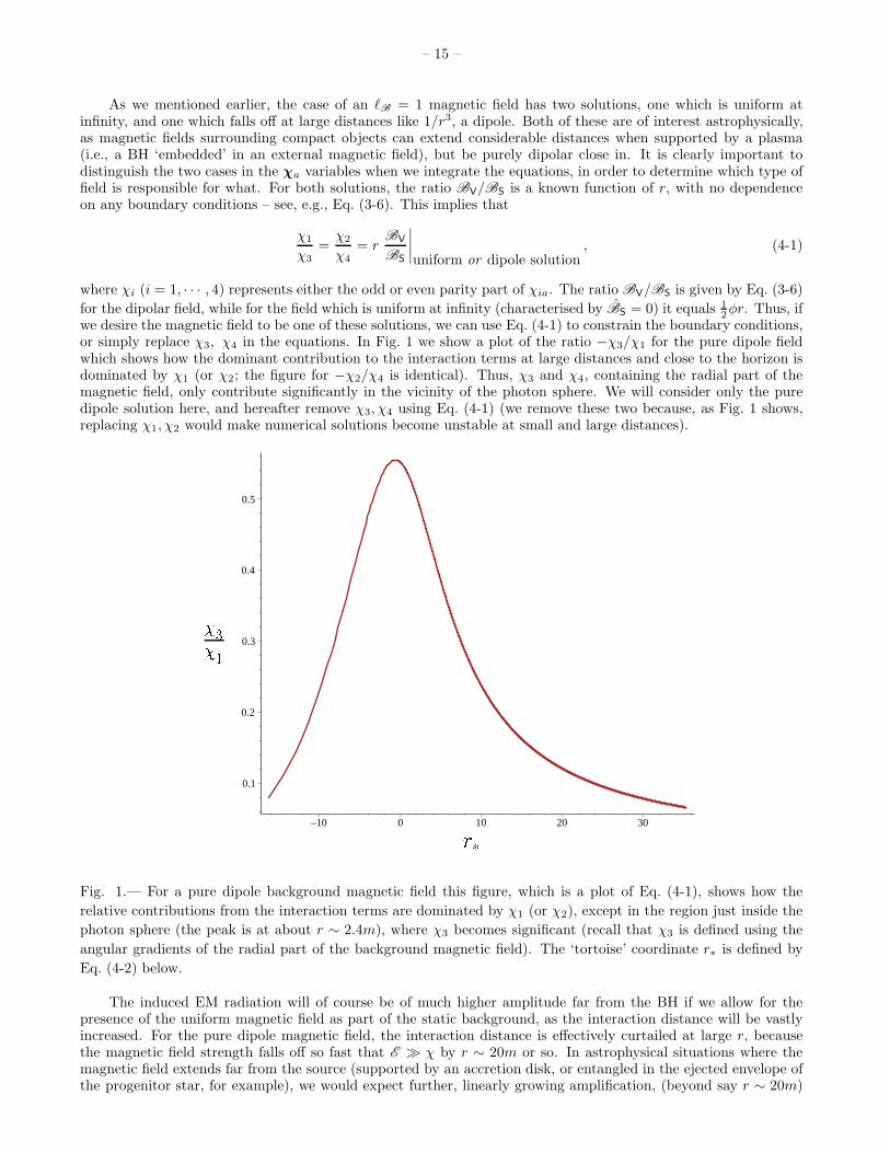
we desire the magnetic field to be one of these solutions, we can use Eq. (4-1) to constrain the boundary conditions,or simply replace χ3, χ4 in the equations. In Fig. 1 we show a plot of the ratio −χ3/χ1 for the pure dipole fieldwhich shows how the dominant contribution to the interaction terms at large distances and close to the horizon isdominated by χ1 (or χ2; the figure for −χ2/χ4 is identical). Thus, χ3 and χ4, containing the radial part of themagnetic field, only contribute significantly in the vicinity of the photon sphere. We will consider only the puredipole solution here, and hereafter remove χ3, χ4 using Eq. (4-1) (we remove these two because, as Fig. 1 shows,replacing χ1, χ2 would make numerical solutions become unstable at small and large distances).
r
3
1
0.1
0.2
0.3
0.4
0.5
–10 0 10 20 30
Fig. 1.— For a pure dipole background magnetic field this figure, which is a plot of Eq. (4-1), shows how the
relative contributions from the interaction terms are dominated by χ1 (or χ2), except in the region just inside the
photon sphere (the peak is at about r ∼ 2.4m), where χ3 becomes significant (recall that χ3 is defined using the
angular gradients of the radial part of the background magnetic field). The ‘tortoise’ coordinate r∗ is defined by
Eq. (4-2) below.
The induced EM radiation will of course be of much higher amplitude far from the BH if we allow for thepresence of the uniform magnetic field as part of the static background, as the interaction distance will be vastlyincreased. For the pure dipole magnetic field, the interaction distance is effectively curtailed at large r, becausethe magnetic field strength falls off so fast that E ≫ χ by r ∼ 20m or so. In astrophysical situations where themagnetic field extends far from the source (supported by an accretion disk, or entangled in the ejected envelope ofthe progenitor star, for example), we would expect further, linearly growing amplification, (beyond say r ∼ 20m)
– 16 –
over the amplification we report below. This will be studied at a later date when a plasma is included into thediscussion, but should be borne in mind in what follows.
Hereafter we shall set m = 1 (which just defines the units of r), and we shall use the tortoise coordinate r∗ ofRegge and Wheeler (Regge and Wheeler 1957) defined by
dρ = 12φrdr∗ =
(
12φr)−1
dr ⇒ r∗ = r + 2m ln( r
2m− 1)
. (4-2)
Because the system of equations we are investigating are linear, the units we use are physically irrelevant, and istied into the physical amplitude of our initial data which we normalise at unity (so that if units are chosen for χsay we can immediately read off the actual amplitudes for E ).
4.1. The initial value problem
Here we envisage the following situation: at some initial time t = 0 the interaction is ‘turned on’ with sometypical initial profile for the GW [i.e., the tensor Wab, which translates in this case to χa(t = 0) = χa
0], at whichtime the induced EM field is zero, but with non-zero second time derivatives (‘acceleration’). Although intuitivelyreasonable for modeling a situation such as BH formation or where the magnetic field becomes very strong veryquickly, say, we require this switching on of the interaction because otherwise the ME will not be consistent for ageneral χa
0 .A common way of specifying initial data for this type of problem is to consider GW scattering off a BH, with
the initial data given by a static narrow Gaussian peak at some distance from the hole (Andersson 1997). Thisthen splits in two as the RW equation is evolved, with the part falling into the hole of most interest: this scattersoff the photon sphere and starts the black hole vibrating (roughly speaking), with a characteristic waveformwhich is largely independent of the initial data, dominated by the quasi-normal modes of the BH (which onlydepend on its mass) (Andersson 1995, 1997; Sun and Price 1998; Nollert 1999). We will use this scenario withW0 ∼ exp
(
−(r∗ − 20)2)
at t = 0, which we normalise so that at t = 0 and r∗ = 20, χ1V = 1. We will not consider apulse originating further from the hole because the dipole field falls off so fast with distance; the qualitative resultsremain the same.
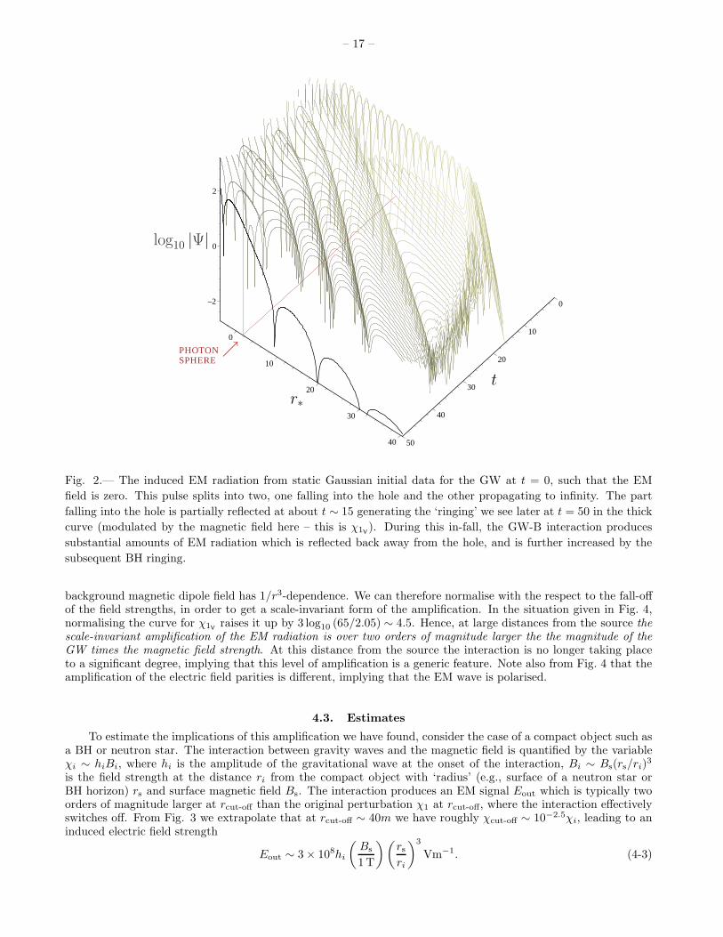
We then evolve our key equation (3-41) and the wave equation for χ1 [modified by replacing χ3 with Eq. (4-1)as discussed above] with this initial data. This then gives the solution for WS, which we convert to EV. Resultsare shown in Figs. (2) and (3) for log10 |EV|. These figures show the EM radiation generated and subsequentlyamplified during the scattering of the GW off the photon sphere. The ringing of the BH then generates a continuousstream of EM radiation, which at its peak is over two orders of magnitude larger than the initial pulse of radiation(by the time it is reflected back out to r∗ = 20). This radiation mirrors very closely the GW waveform making ita suitable EM counterpart for GW emission.
4.2. The quasi-normal mode approach
We shall now integrate the equations in the frequency domain, summing over the QNMs of the BH, which willtell us about the strength of the interaction in the latter stages of a perturbation of a BH independently of the initialperturbation (Andersson 1997). We imagine that the interaction starts at t = 0 at some inner radius r0, so for r < r0we assume that ES = βS = 0, while χ does its own thing; at r = r0 we choose boundary conditions for each ωn suchthat all EM terms and their derivatives are equal to zero; for want of accurate boundary conditions for the GW, werandomly4 choose χ(ωn) = χ0. In order to compare differing amplifications for each parity, we use the same χ0 forboth parities. We then integrate Eqs. (3-45a) – (3-45) out to some r = rmax for each QNM frequency ωn. Then,for each variable at r = rmax we can simply add up the QNMs. This then gives a good approximation to the timedecay of the signal as it passes r = rmax after t >
∼ tmax = rmax− r0+2m ln [(rmax − 2m) / (r0 − 2m)] (Andersson1997; Nollert 1999). We use the first twelve QNM frequencies as tabulated in Nollert and Schmidt (1992) forσn = 1
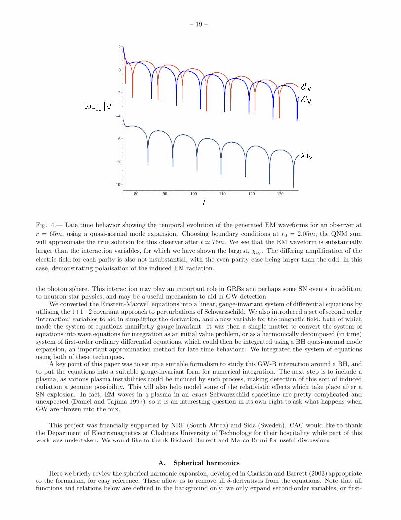
2φrωn – see Eq. (3-18).In Figure 4 we show a typical result of this integration, for an observer situated at r ≃ 65, with r0 = 2.05.
The generated electric field is shown, for both parities, as is the largest interaction variable, which is χ1V in thiscase. The units of the graph are arbitrary: dividing each variable by |χ0| (to make each variable dimensionless),say, will merely shift all the curves up or down. At large distances from the source, the behaviour of the fields canbe represented as an amplitude over a potential of the distance function. In the case of the gravitational wave,the fall-off scales like 1/r, while for a spherical electromagnetic wave it behaves as 1/r. At the same time, the
4Although this may seem somewhat arbitrary, it is no more arbitrary than choosing a Gaussian distribution as in the last section.
We have performed the numerical integration below for many different choices of χ0, and the results are qualitatively similar.
– 17 –
t
r∗
PHOTONրSPHERE
log10 |Ψ|
0
10
20
30
40
50
0
10
20
30
40
–2
0
2
Fig. 2.— The induced EM radiation from static Gaussian initial data for the GW at t = 0, such that the EM
field is zero. This pulse splits into two, one falling into the hole and the other propagating to infinity. The part
falling into the hole is partially reflected at about t ∼ 15 generating the ‘ringing’ we see later at t = 50 in the thick
curve (modulated by the magnetic field here – this is χ1V). During this in-fall, the GW-B interaction produces
substantial amounts of EM radiation which is reflected back away from the hole, and is further increased by the
subsequent BH ringing.
background magnetic dipole field has 1/r3-dependence. We can therefore normalise with the respect to the fall-offof the field strengths, in order to get a scale-invariant form of the amplification. In the situation given in Fig. 4,normalising the curve for χ1V raises it up by 3 log10 (65/2.05) ∼ 4.5. Hence, at large distances from the source thescale-invariant amplification of the EM radiation is over two orders of magnitude larger the the magnitude of theGW times the magnetic field strength. At this distance from the source the interaction is no longer taking placeto a significant degree, implying that this level of amplification is a generic feature. Note also from Fig. 4 that theamplification of the electric field parities is different, implying that the EM wave is polarised.
4.3. Estimates
To estimate the implications of this amplification we have found, consider the case of a compact object such asa BH or neutron star. The interaction between gravity waves and the magnetic field is quantified by the variableχi ∼ hiBi, where hi is the amplitude of the gravitational wave at the onset of the interaction, Bi ∼ Bs(rs/ri)
3
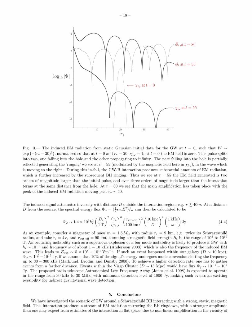
is the field strength at the distance ri from the compact object with ‘radius’ (e.g., surface of a neutron star orBH horizon) rs and surface magnetic field Bs. The interaction produces an EM signal Eout which is typically twoorders of magnitude larger at rcut-off than the original perturbation χ1 at rcut-off, where the interaction effectivelyswitches off. From Fig. 3 we extrapolate that at rcut-off ∼ 40m we have roughly χcut-off ∼ 10−2.5χi, leading to aninduced electric field strength
Eout ∼ 3× 10⁸hi
(
Bs
1T
)(
rsri
)3
Vm−1. (4-3)
– 18 –
χ1Vat t = 55
EV at t = 55
EV at t = 80
←− χ1Vat t = 0
r∗
log10 |Ψ|
–3
–2
–1
0
1
2
10 20 30 40
Fig. 3.— The induced EM radiation from static Gaussian initial data for the GW at t = 0, such that W ∼
exp(
−(r∗ − 20)2)
, normalised so that at t = 0 and r∗ = 20, χ1V = 1; at t = 0 the EM field is zero. This pulse splits
into two, one falling into the hole and the other propagating to infinity. The part falling into the hole is partially
reflected generating the ‘ringing’ we see at t = 55 (modulated by the magnetic field here in χ1V), in the wave which
is moving to the right . During this in-fall, the GW-B interaction produces substantial amounts of EM radiation,
which is further increased by the subsequent BH ringing. Thus we see at t = 55 the EM field generated is two
orders of magnitude larger than the initial pulse, and over three orders of magnitude larger than the interaction
terms at the same distance from the hole. At t = 80 we see that the main amplification has taken place with the
peak of the induced EM radiation moving past r∗ ∼ 40.
The induced signal attenuates inversely with distance D outside the interaction region, e.g. r & 40m. At a distanceD from the source, the spectral energy flux Φω = (12ǫ0cE
2)/ω can then be calculated to be
Φω ∼ 1.4× 10⁶h2i
(
Bs
1T
)2(rsri
)6( rcut-off100 km
)2(
10 kpc
D
)2(1 kHz
ω
)
Jy. (4-4)
As an example, consider a magnetar of mass m = 1.5M⊙ with radius rs = 9 km, e.g. twice its Schwarzschildradius, and take ri = 4 rs and rcut-off = 90 km, assuming a magnetic field strength Bs in the range of 105 to 1010
T. An occurring instability such as a supernova explosion or a bar mode instability is likely to produce a GW withhi ∼ 10−3 and frequency ω of about 1− 10 kHz (Andersson 2003), which is also the frequency of the induced EMwave. This leads to Eout ∼ 5 × 10⁸ − 1013Vm−1. If such an event happened within our galaxy (D ∼ 10 kpc),Φω ∼ 105− 1015 Jy, if we assume that 10% of the signal’s energy undergoes mode conversion shifting the frequencyup to 30− 300 kHz (Marklund, Brodin, and Dunsby 2000). To achieve a higher detection rate, one has to gatherevents from a farther distance. Events within the Virgo Cluster (D ∼ 15 Mpc) would have flux Φf ∼ 10−1 − 109
Jy. The proposed radio telescope Astronomical Low Frequency Array (Jones et al. 1998) is expected to operatein the range from 30 kHz to 30 MHz, with minimum detection level of 1000 Jy, making such events an excitingpossibility for indirect gravitational wave detection.
5. Conclusions
We have investigated the scenario of GW around a Schwarzschild BH interacting with a strong, static, magneticfield. This interaction produces a stream of EM radiation mirroring the BH ringdown, with a stronger amplitudethan one may expect from estimates of the interaction in flat space, due to non-linear amplification in the vicinity of
– 19 –
E
V
E
V
1
V
t
log
10
jj
–10
–8
–6
–4
–2
0
2
80 90 100 110 120 130
Fig. 4.— Late time behavior showing the temporal evolution of the generated EM waveforms for an observer at
r = 65m, using a quasi-normal mode expansion. Choosing boundary conditions at r0 = 2.05m, the QNM sum
will approximate the true solution for this observer after t ≃ 76m. We see that the EM waveform is substantially
larger than the interaction variables, for which we have shown the largest, χ1V . The differing amplification of the
electric field for each parity is also not insubstantial, with the even parity case being larger than the odd, in this
case, demonstrating polarisation of the induced EM radiation.
the photon sphere. This interaction may play an important role in GRBs and perhaps some SN events, in additionto neutron star physics, and may be a useful mechanism to aid in GW detection.
We converted the Einstein-Maxwell equations into a linear, gauge-invariant system of differential equations byutilising the 1+1+2 covariant approach to perturbations of Schwarzschild. We also introduced a set of second order‘interaction’ variables to aid in simplifying the derivation, and a new variable for the magnetic field, both of whichmade the system of equations manifestly gauge-invariant. It was then a simple matter to convert the system ofequations into wave equations for integration as an initial value problem, or as a harmonically decomposed (in time)system of first-order ordinary differential equations, which could then be integrated using a BH quasi-normal modeexpansion, an important approximation method for late time behaviour. We integrated the system of equationsusing both of these techniques.
A key point of this paper was to set up a suitable formalism to study this GW-B interaction around a BH, andto put the equations into a suitable gauge-invariant form for numerical integration. The next step is to include aplasma, as various plasma instabilities could be induced by such process, making detection of this sort of inducedradiation a genuine possibility. This will also help model some of the relativistic effects which take place after aSN explosion. In fact, EM waves in a plasma in an exact Schwarzschild spacetime are pretty complicated andunexpected (Daniel and Tajima 1997), so it is an interesting question in its own right to ask what happens whenGW are thrown into the mix.
This project was financially supported by NRF (South Africa) and Sida (Sweden). CAC would like to thankthe Department of Electromagnetics at Chalmers University of Technology for their hospitality while part of thiswork was undertaken. We would like to thank Richard Barrett and Marco Bruni for useful discussions.
A. Spherical harmonics
Here we briefly review the spherical harmonic expansion, developed in Clarkson and Barrett (2003) appropriateto the formalism, for easy reference. These allow us to remove all δ-derivatives from the equations. Note that allfunctions and relations below are defined in the background only; we only expand second-order variables, or first-
– 20 –
order variables which form part of a quadratic second-order variable so zeroth-order equations are sufficient.We introduce spherical harmonic functions Q = Q(ℓ,m), with m = −ℓ, · · · , ℓ, defined on the background, such
thatδ2Q = −ℓ (ℓ+ 1) r−2Q, Q = 0 = Q. (A1)
We also need to expand vectors and tensors in spherical harmonics. We therefore define the even (electric) parityvector spherical harmonics for ℓ ≥ 1 as
Q(ℓ)a = rδaQ
(ℓ) ⇒ Qa = 0 = Qa, δ2Qa = (1− ℓ (ℓ+ 1)) r−2Qa; (A2a)
where the (ℓ) superscript is implicit, and we define odd (magnetic) parity vector spherical harmonics as
Q(ℓ)a = rεabδ
bQ(ℓ) ⇒ ˆQa = 0 = ˙Qa, δ2Qa = (1− ℓ (ℓ+ 1)) r−2Qa. (A2b)
Note that Qa = εabQb ⇔ Qa = −εabQ
b, so that εab is a parity operator. The crucial difference between these twotypes of vector spherical harmonics is that Qa is solenoidal, so
δaQa = 0, while δaQa = −ℓ (ℓ+ 1) r−1Q. (A3)
Note also thatεabδ
aQb = 0, and εabδaQb = ℓ (ℓ+ 1) r−1Q. (A4)
The harmonics are orthogonal: QaQa = 0 (for each ℓ). Similarly we define even and odd tensor spherical harmonicsfor ℓ ≥ 2 as
Qab = r2δaδbQ, ⇒ Qab = 0 = Qab, δ2Qab =[
φ2 − 3E − ℓ (ℓ+ 1) r−2]
Qab; (A5a)
and
Qab = r2εcaδcδbQ, ⇒ ˆQab = 0 = ˙Qab, δ2Qab =
[
φ2 − 3E − ℓ (ℓ+ 1) r−2]
Qab, (A5b)
which are orthogonal: QabQab = 0, and are parity inversions of one another: Qab = −εcaQ
cb ⇔ Qab = εcaQ
cb .
We can now expand any second-order scalar Ψ in terms of these functions as
Ψ =∞∑
ℓ=0
m=ℓ∑
m=−ℓ
Ψ(ℓ,m)S
Q(ℓ,m) = ΨSQ, (A6)
where the sum over ℓ and m is implicit in the last equality. The S subscript reminds us that Ψ is a scalar, andthat a spherical harmonic expansion has been made. Due to the spherical symmetry of the background, m neverappears in any equation so we can just ignore it. Any second-order vector Ψa can now be written
Ψa =
∞∑
ℓ=1
Ψ(ℓ)VQ(ℓ)
a + Ψ(ℓ)VQ(ℓ)
a = ΨVQa + ΨVQa. (A7)
Again, we implicitly assume a sum over ℓ in the last equality, and the V reminds us that Ψa is a vector expandedin spherical harmonics. Any second-order tensor may be also be expanded
Ψab =
∞∑
ℓ=2
Ψ(ℓ)TQ
(ℓ)ab + Ψ
(ℓ)TQ
(ℓ)ab = ΨTQab + ΨTQab. (A8)
Further useful identities are to be found in Clarkson and Barrett (2003).
REFERENCES
Acernese, F., et al. 2002, Class. Quantum Grav., 19, 1421
Alcubierre, M., and Masso, J. 1998, Phys. Rev. D, 57, 4511
Andersson, N. 1995, Phys. Rev. D, 51, 353
Andersson, N. 1997, Phys. Rev. D, 55, 468
Andersson, N. 2003, Class. Quantum Grav., 20, R105
Ando, M., et al. 2002, Class. Quantum Grav., 19, 1409
– 21 –
Barish, B., and Weiss, R. 1999, Phys. Today, 52, 44
Brodin, G., and Marklund, M. 1999, Phys. Rev. Lett., 82, 3012
Brodin, G., Marklund, M., and Servin, M. 2001, Phys. Rev. D, 63, 124003
Bruni, M., Matarrese, S., Mollerach, S., and Sonego, S. 1997, Class. Quantum Grav., 14, 2585
Bruni, M., and Sonego, S. 1999, Class. Quantum Grav., 16, L29
Buonanno, A. 2002, Class. Quantum Grav., 19, 1267
Cardoso, V., Lemos, J. P. S., and Yoshida, S. 2003, gr-qc/0307104
Cardoso, V. and Lemos, J. P. S. 2003, Phys. Rev. D, 67 084005
Cardoso, V. and Lemos, J. P. S. 2003, Gen. Rel. Grav., 35 L327
Cardoso, V. and Lemos, J. P. S. 2002, Phys. Lett. B 538 1
Chandrasekhar, S. 1983, The Mathematical Theory of Black Holes, Oxford: Oxford University Press
Cooperstock, F. I. 1968, Ann. Phys., 47, 173
Clarkson, C. A., and Barrett, R. K. 2003, Class. Quantum Grav., 20, 3855
Daniel, J., and Tajima, T. 1997, Phys. Rev. D, 55, 5193
Ellis, G. F. R., and Bruni, M. 1989, Phys. Rev. D, 40, 1804
Ellis, G. F. R., and van Elst, H. 1998, in Theoretical and Observational Cosmology, M. Lachieze-Rey (ed.), NATOScience Series, Kluwer Academic Publishers (gr-qc/9812046v4)
Flanagan, E. E., and Hughes, S. A. 1998a, Phys. Rev. D, 57 4535
Flanagan, E. E., and Hughes, S. A. 1998b, Phys. Rev. D, 57 4566
Gerlach, U. N. 1974, Phys. Rev. Lett., 32, 1023
Jones, D. L., et al. 1998, in ASP Conf. Ser. 144 Radio Emission from Galactic and Extragalactic Compact Sources(eds.) Zensus J A, Taylor G B and Wrobel J M (San Francisco, ASP), 393
Kokkotas, K. D., and Schmidt, B. G. 1999, Living Rev. Relativity, 2, 2(http://www.livingreviews.org/Articles/Volume2/1999-2kokkotas/)
Kouveliotou, C., et al. 1998, Nature, 393 235
Macedo, P. G., and Nelson, A. H. 1983, Phys. Rev. D, 28, 2382
Marklund, M., Brodin, G., and Dunsby, P. K. S. 2000, ApJ, 536, 875
Misner, C. W., Thorne, K. S., and Wheeler, J. A. 1973, Gravitation, San Francisco: W. H. Freeman
Mosquera Cuesta, H. J. 2002, Phys. Rev. D, 65, 064009
Nicholson, D., and Vecchio, A. 1998, Phys. Rev. D, 57, 4588
Nollert, H-P. 1999, Class. Quantum Grav., 16, R159
Nollert, H-P., and Schmidt, B. G. 1992, Phys. Rev. D, 45, 2617
Price, R. H. 1972, Phys. Rev. D, 5, 2439
Price, R. H., and Pullin, J. 1994, Phys. Rev. Lett., 72, 3297
Regge, T., and Wheeler, J. A. 1957, Phys. Rev., 108, 1063
Ruoff, J., Stavridis, A., and Kokkotas, K. D. 2001, gr-qc/0109065; ibid, gr-qc/0203052
Servin, M., and Brodin, G. 2003, Phys. Rev. D, 68, 044017
Servin, M., Brodin, G., and Marklund, M. 2001, Phys. Rev. D, 64, 024013
Stewart, J. M., and Walker, M. 1974, Proc. R. Soc. London A, 431, 49
Sun, Y., and Price, R. H. 1988, Phys. Rev. D, 38, 1040
Sylvestre, J. 2003, ApJ, 591, 1152
Thorne, K. S. 1980, Rev. Mod. Phys., 52, 299
van Putten, M. 2001, Phys. Rev. Lett., 87, 091101
Willke, B., et al. 2002, Class. Quantum Grav., 19, 1377
This preprint was prepared with the AAS LATEX macros v5.2.