Embed Size (px)
Citation preview

MIT/WHOI 97-05
Massachusetts Institute of Technology Woods Hole Oceanographic Institution
Joint Program in Oceanography/
Applied Ocean Science
and Engineering
,o*nG%, %
1930
DOCTORAL DISSERTATION
Larval Dispersal Between Hydrothermal Vent Habitats
February 1996
19970609 092 DHC QUALITY INSPECTED 1

MIT/WHOI 97-05
Larval Dispersal Between Hydrothermal Vent Habitats
by
Stacy L. Kim
Massachusetts Institute of Technology Cambridge, Massachusetts 02139
and
Woods Hole Oceanographic Institution Woods Hole, Massachusetts 02543
February 1996
DOCTORAL DISSERTATION
Funding was provided by the Ocean Ventures Fund of the Woods Hole Oceanographic Institution, the Seaspace/Houston Underwater Club, the Mellon Foundation and the National Science
Foundation through Grant Nos. OCE90-19575 and OCE93-15554.
Reproduction in whole or in part is permitted for any purpose of the United States Government. This thesis should be cited as: Stacy L. Kim, 1996. Larval Dispersal Between Hydrothermal Vent
Habitats. Ph.D. Thesis. MIT/WHOI, 97-05.
Approved for publication; distribution unlimited.
Approved for Distribution:
Laurence P. Madin, Chair
Department of Biology
Marcia K. McNutt MIT Director of Joint Program
John W. Farrington WHOI Dean of Graduate Studies

LARVAL DISPERSAL BETWEEN HYDROTHERMAL VENT HABITATS
by
Stacy L. Kim
B.S., Biological Science University of California, Los Angeles, 1983
M.S., Marine Science Moss Landing Marine Laboratories-San Jose State University, 1989
submitted in partial fulfillment of the requirements for the degree of
DOCTOR OF PHILOSOPHY IN BIOLOGICAL OCEANOGRAPHY
at the
WOODS HOLE OCEANOGRAPHIC INSTITUTION
and the
MASSACHUSETTS INSTITUTE OF TECHNOLOGY
January 1996
© Stacy L. Kim 1996
The author hereby grants to WHOI and MIT permission to reproduce and to distribute copies of this thesis in whole or in part.
Signature of Author MIT-WHOI Joint Program in Biological Oceanography
Certified by 7^^ /^ ^ Lauren S. Mullineaux Associate Scientist, Department of Biology, WHOI
Thesis Supervisor
-^
Accepted bv htFncJcl /**? U^£&^<f^>^. Donald M. Anderson
Chairman, Joint Committee for Biological Oceanography Massachusetts Institute of Technology-Woods Hole Oceanographic Institution


TABLE OF CONTENTS
List of Figures _4
Abstract 5
Acknowledgments 6
Chapter 1. Introduction 7
Chapter 2. Larval Dispersal via Entrainment into Hydrothermal Vent Plumes 25
Chapter 3. Identification of Archaeogastropod Larvae from a Hydrothermal Vent
Community 36
Chapter 4. A Cellular Automata Model of Larval Dispersal and Population
Persistence at Hydrothermal Vent Habitats 66
Chapter 5. Summary 107

LIST OF FIGURES
Chapter 1. Introduction Figure 1. Geological organization of hydrothermal vents.
Chapter 2. Larval Dispersal via Entrainment into Hydrothermal Vent Plumes Figure 1. Schematic diagram of the hydrothermal chimney and plume. Figure 2. Schematic diagram of dye injection system. Figure 3. Calibration of voltage readings from the in-situ fluorometer. Figure 4. Observed and predicted fluorescein concentrations in the plume. Figure 5. Maximum and average dye concentrations observed and predicted.
Chapter 3. Identification of Archaeogastropod Larvae from a Hydrothermal Vent Community
Figure 1. Larvae and juveniles in family Peltospiridae. Figure 2. Larval ?Melanodrymia spp. and juvenile Melanodrymia aurantiaca . Figure 3. Larval and juvenile archaeogastropods. Figure 4. Larval and juvenile Lepetodrilus. Figure 5. Representative examples of pelagic pteropods and heteropods. Figure 6. Larvae of non-vent, benthic species.
Chapter 4. A Cellular Automata Model of Larval Dispersal and Population Persistence at Hydrothermal Vent Habitats
Figure 1. The local neighborhood of 9 cells in the cellular automata. Figure 2. Transition pathways for the cellular automaton model. Figure 3. Schematic of stable distribution of vents. Figure 4. The average number of colonizing larvae reaching a cell. Figure 5. Representative time series of model results. Figure 6. The effects of disturbance probabilities on proportion producing. Figure 7. The effects of survival and global dispersal on proportion producing. Figure 8. The effects of larval supply and global dispersal on proportion
producing. Figure 9. The effects of larval supply and survival on proportion producing. Figure 10. The effects of delayed maturity on proportion producing. Figure 11. Combinations of global dispersal and survival that result in greater
than 50% proportion producing habitat. Figure 12. The effects of disturbance probabilities on colonization rate. Figure 13. The effects of survival and global dispersal on colonization rate. Figure 14. The effect of larval supply and global dispersal on colonization rate. Figure 15. The effect of larval supply and survival on colonization rate.
Chapter 5. Summary Figure 1. Top view of the volume entrained into a central buoyant plume. Figure 2. Side view of the volume entrained into a central buoyant plume.
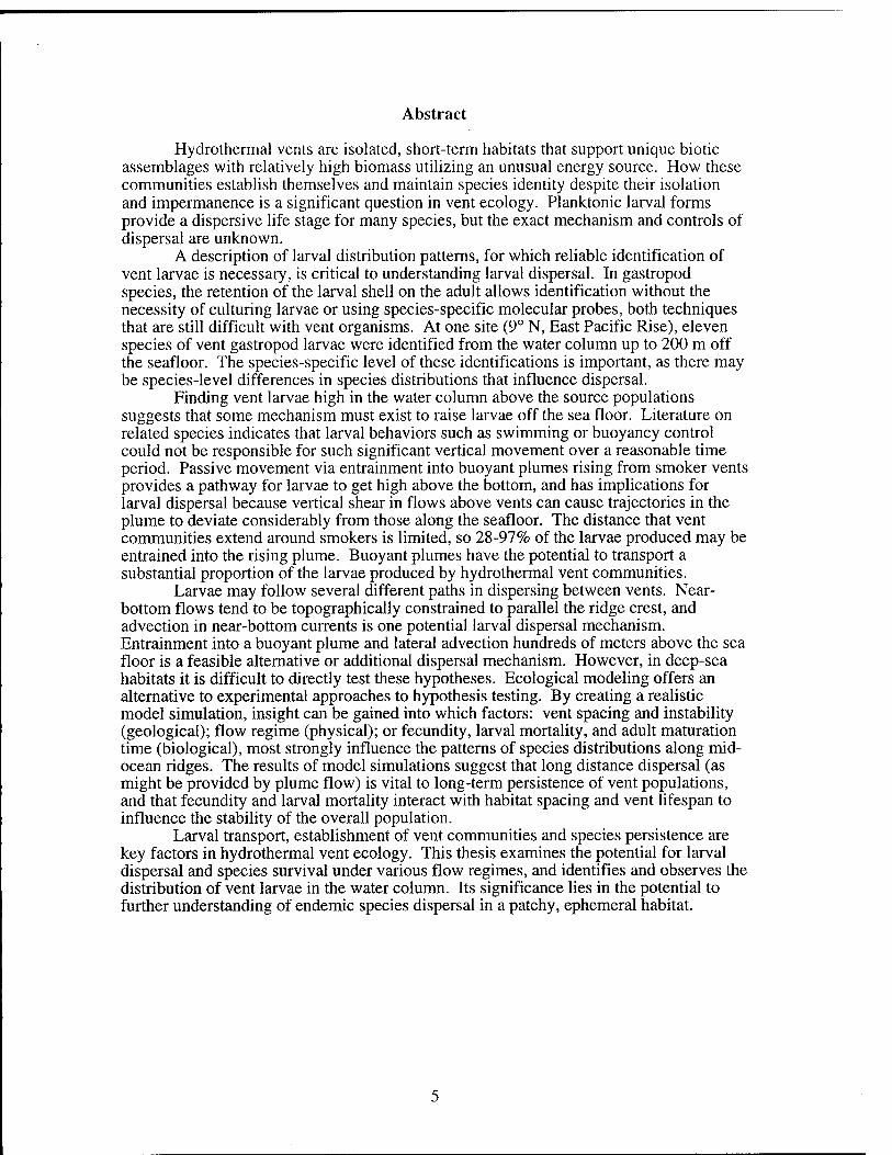
Abstract
Hydrothermal vents are isolated, short-term habitats that support unique biotic assemblages with relatively high biomass utilizing an unusual energy source. How these communities establish themselves and maintain species identity despite their isolation and impermanence is a significant question in vent ecology. Planktonic larval forms provide a dispersive life stage for many species, but the exact mechanism and controls of dispersal are unknown.
A description of larval distribution patterns, for which reliable identification of vent larvae is necessary, is critical to understanding larval dispersal. In gastropod species, the retention of the larval shell on the adult allows identification without the necessity of culturing larvae or using species-specific molecular probes, both techniques that are still difficult with vent organisms. At one site (9° N, East Pacific Rise), eleven species of vent gastropod larvae were identified from the water column up to 200 m off the seafloor. The species-specific level of these identifications is important, as there may be species-level differences in species distributions that influence dispersal.
Finding vent larvae high in the water column above the source populations suggests that some mechanism must exist to raise larvae off the sea floor. Literature on related species indicates that larval behaviors such as swimming or buoyancy control could not be responsible for such significant vertical movement over a reasonable time period. Passive movement via entrainment into buoyant plumes rising from smoker vents provides a pathway for larvae to get high above the bottom, and has implications for larval dispersal because vertical shear in flows above vents can cause trajectories in the plume to deviate considerably from those along the seafloor. The distance that vent communities extend around smokers is limited, so 28-97% of the larvae produced may be entrained into the rising plume. Buoyant plumes have the potential to transport a substantial proportion of the larvae produced by hydrothermal vent communities.
Larvae may follow several different paths in dispersing between vents. Near- bottom flows tend to be topographically constrained to parallel the ridge crest, and advection in near-bottom currents is one potential larval dispersal mechanism. Entrainment into a buoyant plume and lateral advection hundreds of meters above the sea floor is a feasible alternative or additional dispersal mechanism. However, in deep-sea habitats it is difficult to directly test these hypotheses. Ecological modeling offers an alternative to experimental approaches to hypothesis testing. By creating a realistic model simulation, insight can be gained into which factors: vent spacing and instability (geological); flow regime (physical); or fecundity, larval mortality, and adult maturation time (biological), most strongly influence the patterns of species distributions along mid- ocean ridges. The results of model simulations suggest that long distance dispersal (as might be provided by plume flow) is vital to long-term persistence of vent populations, and that fecundity and larval mortality interact with habitat spacing and vent lifespan to influence the stability of the overall population.
Larval transport, establishment of vent communities and species persistence are key factors in hydrothermal vent ecology. This thesis examines the potential for larval dispersal and species survival under various flow regimes, and identifies and observes the distribution of vent larvae in the water column. Its significance lies in the potential to further understanding of endemic species dispersal in a patchy, ephemeral habitat.

Acknowledgments
A lot of people helped me survive this thesis. It's a very diverse group of people: those who kept me sane, those who drove me crazy and those that I drove crazy.
I thank Lauren Mullineaux for being not only an excellent advisor, but also a wonderful role model. Karl Helfrich for his patience. Rudi Scheltema for his wisdom. Heidi Nepf, Hal Caswell, and Ron Etter for all their time and efforts. Peter Wiebe, Philippe Bouchet, Alan Pooley, Michael Moore, Rich Lutz, Dave Caron, Anders Waren, Al Pleuddemann, Roger Samelson, Mark Benfield and Aanderaa Instruments for explaining things and letting me use their stuff. The Ocean Ventures Fund, Seaspace/Houston Underwater Club, and most of all, WHOI Education for keeping me fed.
And from my heart I am grateful to Kendall Banks for trying. My best friends, Craig Lewis for everything, and Ewann Agenbroad for everything plus chocolate. The cast and crew of the All and Alvin, especially Spaceman Dave and BLee and King Pat, for sending me email and making me laugh. Carin Ashjian for being silly. Bonnie Ripley for being strong. Susan Mills, and Steve and Guy and Lisi, for reality checks. Andrea Arenovski and Doug Hersh for showing me it can be done. Ami Scheltema, Sarah Little, Constance Grämlich, Julie Pallant, Beth Anderson, Agnes Debrunner, Jill Johnen nee Schoenherr, Cid Richards and Kathleen Stacey for being bright stars that kept me reaching. Rycz Pawlowiczfich, Alan Kuo, Lisa Garland, Hovey Clifford, Spawn Doan, Mari Butler and Mary Landsteiner, KT Scott, Tim Conners, Patty Rosel and Scott France and Laika and Quessa, Erich Horgan, Diane DiMasse, Melora Samelson, Jim Craddock, Rich Harbison and 'Winkle, Paul Dunlap and Theo, George Hampson and Ethel LeFave for smiles/hugs/licks. Tubby Lindner for making me look good. And Club Tub et al.: Dale, Deb, Melissa, Brad, Rick and Cyndy, Rod and Kathy, Bob and Donna, Gorka, John, Vicki, Brenda, Joanne, Lori, Phil, Scott, Aaron, and Saralyn, for sand in my shorts. Everybody who tried underwater hockey. Especially the home team: Steve Shephard, Sarah Zimmerman, Tim and Kelly Burke, Laura Praderio, Dave Fernandes, Stefan Hussenoeder, Danny Sigman, and Miles Sundermeyer, and the away team: Carol, Woody, Party Dan, Ducklet, RickeyRickey, FLMB Claire, Dick 'n' Dot, Brigit and Mike, Uncle Terry and MoJo. All the owls - security guards, cleaning crew, and Dan Smith for sharing late nights. Everyone who wants me to come home, especially Oliver and Jo, Di, Don, Baldo, Eric, Jim, and Alan and Sheila. And always, Mom and Ethan.

Chapter 1
Introduction
GENERAL
Introduction
Hydrothermal vents are short-lived islands of habitat scattered along mid-ocean
ridges. Vents are small areas where hydrothermal fluid flows from the seafloor; this fluid
is at high temperatures and contains reduced chemicals that act as a food source for dense
communities of specialized organisms. Each vent "island" has a limited area, on the order
of square meters, and provides habitat for many species that are unable to survive away
from vent influence. The same megafaunal species are found at vents separated by
hundreds to thousands of meters of sea-floor. As in other island-restricted species (e.g.
ants, MacArthur and Wilson 1967), there must be migration between vents to maintain
species identity as a single interbreeding population over successive generations. This
thesis examines dispersal between the patchily distributed vent habitats in the deep sea.
Although individual vents are ephemeral, some lasting only decades, the
hydrothermal habitat in general persists through geologic time (Haymon et al. 1984, Gage
and Tyler 1991). Vent species must cope with temporal as well as spatial patchiness, and
must be able to colonize new vents as they open, or the closing of old vents will result in
eventual species extinction.
Many of the megafaunal species found at vents are sessile and migration by the
adults is impossible. In related marine invertebrate species, planktonic larvae provide a
means of dispersal. Larvae of many vent species are planktonic and may serve a similar
function, a life stage that can be transported across the unsuitable habitat between vents.
However, this solution raises further questions. How do tiny, planktonic life stages
traverse the distances between vents? Are there mechanisms for larval transport to, and
settling in, the small, isolated patches of suitable habitat? Planktonic larvae may be the

means, but the mechanisms by which vent species disperse and persist are not presently
understood.
The objectives of this thesis are to answer three general questions:
1) What is the contribution of different physical mechanisms to larval dispersal of endemic
vent species?
Near-bottom flows and/or diffusive motion are potential larval dispersal mechanisms.
Is it possible that entrainment into buoyant plumes rising from hydrothermal vents can
provide another dispersal mechanism?
2) What dispersal patterns are necessary to maintain existing species distributions?
Is local dispersal enough to ensure transport between existing or to newly opened vent
habitats? Is global dispersal required for species continuity across large spatial scales?
3) What are the effects of habitat and population patchiness on metapopulation
persistence?
How do dispersal capabilities interact with population distributions to influence
population persistence? How does this process vary with different habitat
distributions?
Approaches
I address these question using three approaches. First, I test a standard plume
model to determine whether vent plumes can entrain substantial numbers of larvae of vent
organisms and are potentially important as a dispersal mechanism. Then I use scanning
electron microscopy to identify the species of larvae collected near vents, a vital initial step
in defining larval distributions and dispersal patterns. Finally, I utilize an ecological model
to examine spatial and temporal habitat distribution, dispersal route, population maturation,
fecundity, and larval survival as factors influencing population dynamics in a patchy
habitat.

Buoyant Plumes
A standard model that describes the behavior of buoyant plumes is given in Turner
(1973), but plumes at hydrothermal vents may behave differently from the theoretical
predictions of this standard model. The standard model defines a single buoyancy source,
hydrothermal vents may have several apertures very close together that contribute to a
single plume. Initial momentum in standard model is defined as zero, real plumes have
initial momentum and behave as buoyant jets close to the source. The model assumes that
there is no volume change as the plume rises, this is not true for vent plumes (Little et al.
1987). To determine whether it is realistic to use predictions of the plume model to
estimate the degree of influence a vent plume may have on dispersal of hydrothermal vent
organisms, it is important to test the model predictions in the field. In this case, whether
the model satisfactorily predicts the degree of entrainment of particles, or larvae, external to
the plume is of concern. If idealized plume and hydrothermal vent plume behavior match
well, the theoretical model can be used to predict the potential importance of buoyant
plumes at hydrothermal vents to larval dispersal.
Larval Identification
Invertebrate larvae are found ubiquitously in the water column, but make up only a
small proportion of the plankton near vents (Mullineaux et al. 1995). To be able to define
larval distribution patterns, it must be determined whether these larvae are of vent origin.
Larval distribution patterns will help ascertain which dispersal pathways are utilized
successfully by vent species. Larvae may become entrained into buoyant plumes, or may
remain in near-bottom waters, but only those that remain viable during transport are
important to colonization processes. Identification to species is vital, for there may be
species-specific larval distribution patterns that have implications for individual species
success at colonizing or maintaining populations. Larval identification techniques,

allowing recognition of larvae of vent species wherever they are found, are thus crucial to
understanding dispersal between vent habitats.
Modeling
Mathematical modeling of the ecological system is another approach to
understanding dispersal processes at hydrothermal vents. Modeling can be used to indicate
the relative importance of factors such as dispersal mechanisms, habitat distributions, or
biological limitations to population distributions at vents. Larvae that are transported in
near-bottom flows or that are entrained into a rising plume will undergo different dispersal
directions and speeds in accordance with flow patterns that occur at the different heights
above the bottom. Though I cannot directly watch where specific larvae go in the field, I
can, through the use of appropriate ecological models, determine whether particular
physical and biological mechanisms could result in the population distribution patterns
observed across vent habitat distributions. This approach will help clarify the spatial and
temporal scales over which the different potential dispersal mechanisms are important to
larval dispersal between vents.
Significance
Understanding the mechanisms of dispersal in vent species and their consequences
for vent population dynamics is important because hydrothermal vents are isolated,
ephemeral habitats that support unusual biotic assemblages, and how such communities
establish themselves and maintain species identity is an important ecological question.
Planktonic larval forms provide a dispersive life stage for many species, but the exact
mechanism and controls of dispersal are unknown. My thesis research addresses critical
components of larval dispersal between hydrothermal vent habitats. By creating a model
simulation, the factors that most strongly influence the patterns of species distributions
along mid-ocean ridges: between vent spacing (geological); flow regime (physical); or
10

organism physiology (biological), can be determined. For example, if the dispersal
mechanism strongly affects the patterns the model generates, while larval life span has little
effect on the distribution patterns, it would suggest that further research concentrate on
current regimes and larval distributions in the water column, rather than larval physiology.
Model results can thus be used to clarify and guide further research efforts. The
significance of this work is to further our understanding of dispersal by vent species in a
patchy, ephemeral habitat.
BACKGROUND
Vent Biology
The species found in high abundances at hydrothermal vents are usually restricted
to such an environment. Though a species range may span tens of degrees of latitude, the
smaller scale spatial distribution is as discontinuous as the vent habitat. It has been
hypothesized that one way of maintaining species distributions across the large expanses of
inhospitable habitat between vents is for vent fauna to use whale carcasses as stepping
stones (Smith et al. 1989). The reduced chemicals provided by the decaying whale lipids
may act as an energy source similar to vent chemicals. However, this seems unlikely based
on the very tiny amount of overlap between known vent and carcass faunas (<1%).
Metazoan species found at vents are all dependent to some extent on the abundant
food provided by chemosynthetic bacteria; that in turn depends on the hydrothermal fluid
which carries dissolved hydrogen sulfide and methane. Because of the toxicity of these
chemicals, only species with specific adaptations can exploit this food source.
Additionally, oxygen and hydrogen sulfide cannot coexist; when combined they rapidly
undergo chemical reactions that render each useless for respiration and chemosynthesis
respectively. Organisms must deal with contradictory needs: avoiding the toxic chemicals
and requiring them for the nutrition of the symbionts, needing oxygen for respiration and
avoiding it to keep sulfide available for chemosynthesis. The vestimentiferan worm Riftia
11

does this by partitioning uptake in time, it lives in the highly turbulent zone close to intense
hydrothermal flows and alternately is exposed to oxygen-rich seawater and sulfide-rich
hydrothermal fluid (Johnson et al. 1988). Riftia blood contains proteins which allow it to
bind and carry both oxygen and sulfide from the surrounding waters (Arp and Childress
1981). Calyptogena, the vent clam, partitions resource uptake spatially: the clams live in
crevices with a vascularized foot pushed into hydrothermal fluids, while their siphons
extend into the ambient seawater above (Fisher et al. 1988). This paradoxical dependence
on oxygen and hydrogen sulfide keeps the habitat window of vent species very narrow.
The same set of factors may reduce predation and competition pressures from the
surrounding community because organisms find it difficult to invade the toxic vent habitat.
Larvae of species limited to vent habitats must be capable of sufficient dispersal
between active vents to maintain existing species distributions. Lutz et al. (1980)
suggested that the distribution of vent habitat should select for highly dispersive larval
developmental types. Non-feeding lecithotrophic larvae are, as a rule, short-lived in the
plankton, whereas pianktotrophic larvae remain in the plankton for longer periods and
grow while planktonic. These characteristics suggest that planktotrophs can disperse
further than lecithotrophs. Because of the distances between vent habitats, one might
expect that vent species would have planktotrophic larvae, but many species do not. Both
larval types are found in different vent species, with no corresponding differences in adult
distributions, leading Lutz (1988) to later suggest that dispersal capability is not necessarily
related to developmental type. Developmental type appears phylogenetically constrained,
whereas physiological ability to cope with the rigorous habitat, as well as dispersal
capability, appear to influence which species are found at vents.
The distance that larvae can disperse depends on the duration of the larval phase,
and on the ambient current speeds. Direct measurement of larval survival time has not been
possible in hydrothermal vent species, but comparisons with related planktotrophic shallow
water species suggest a larval survival time on the order of days to months (turrid
12
gastropods 1-7 weeks, Gustaffson et al. 1991; mytilid bivalves 2-4 weeks, Lutz et al.
1980; terebellid polychaetes 3 days, McHugh 1989).
These approximations may underestimate the larval lifespan of vent organisms.
Lutz et al. (1980) have hypothesized that low temperatures may slow the development time
of vent larvae. Development time may also be influenced by food supply, but all else being
equal, decreased temperatures can slow development time to months or even a year as has
been found for other species (Hoegh-Guldberg et al. 1991, Scheltema pers. comm.).
Stepwise dispersal along vent "corridors" may be facilitated by these slowed developmental
rates. Lutz et al. (1984) suggest a dual mechanism, delayed development when larvae drift
into cold water away from a vent, and rapid development if conditions are hospitable.
Although delayed metamorphosis at low temperatures may increase dispersal range, longer
survival times may have little effect on the direction of larval transport.
Whether larvae reach suitable habitat can be influenced by larval behaviors, such as
swimming. Larval behavior can be altered by various cues, such as contact with
appropriate substrates or presence of conspecifics (Crisp 1976). Barnacles and serpulids,
both taxa found at vents, exhibit settlement responses to specific cues (Knight-Jones 1953,
Scheltema et al. 1981). Larvae can remain in the water column after they have achieved
competence, delaying settlement until the presence of a cue results in behavioral changes
and rapid settlement. Since larval behavior in hydrothermal vent species can only be
postulated from behavior of related species, it is simplest to assume neutrally buoyant
larvae that settle all at once after a fixed lifespan. Larval behavior may influence settling
velocity, but the highly simplified assumption of passive larvae is the most straightforward
first-order approximation. This assumption is used in the modeling work presented in
Chapter 2.
Many aspects of biology of vent organisms, such as larval distributions, lifespans,
mortality rates, and settling velocities, cannot be precisely defined, because of the
difficulties of field experimentation in the deep-sea and the problems of maintaining the
13

organisms in the laboratory. An important first step towards defining larval distributions is
taken in this thesis work by identifying vent larvae to species. The relative importance of
other factors to the successful dispersal and persistence of populations can be determined
by using an ecological model. In this way I will examine the larval lifespans and survival
rates that are necessary for persistence of populations in a patchy, ephemeral habitat,
though the model I use is not designed to test larval behavior.
Vent Geology
Mid-ocean ridge systems have characteristic spreading rates that shape their
geomorphology. Fast spreading ridges (>10 cm/year full spreading rate) consist of a
central, axial high with a shield volcano-like cross section and a very narrow central
graben, with frequent high temperature hydrothermal activity. In contrast, slow spreading
ridges (1-5 cm/year) have a large and deep axial rift valley, closely spaced transform faults,
and only occasional hydrothermal venting (MacDonald 1985). The distribution of
hydrothermal habitat at slow spreading ridges is therefore less linear and more widely
spaced than at fast spreading ridges.
A repetitive geologic cycle appears to occur at ridge crests. On fast spreading
ridges the cycle takes approximately a thousand years, on slow spreading ridges it takes
several thousand years. On fast spreading ridges, individual hydrothermal vents are active
for 10-100 years, out of an approximate 1000 years that a ridge section will remain active.
This period is the amount of time it takes for a small magma chamber, such as those
hypothesized to occur under fast spreading ridges, to cool (Humphris 1995). Because of
the frequent occurrence of tectonic activity, faults are continually shifting and vents are
likely to appear anywhere along the ridge crest, though they are concentrated at the edges of
the axial valley. On slow spreading ridges, Sinton and Detrich (1992) envision a
consistent, large zone of crystal mush that maintains activity for tens of thousands of years,
though not continuously. Vents tend to be active for several hundred years, and later
14

reappear in the same location after thousands of years of inactivity. This constancy is
possibly due to the more stable network of fractures that are not disrupted by frequent
tectonic disturbances, allowing upward percolation of the hydrothermal fluid to a consistent
location.
Geologists have described four spatial levels of organization in hydrothermal vent
systems (figure 1). First order segments span areas between transform faults, and are
several hundred kilometers long. Second order segments, on the order of one hundred
kilometers long, are defined as overlapping spreading centers large enough to leave traces
on the ridge flanks as they spread; third order segments are smaller overlapping spreading
centers which do not persist and are tens of kilometers long. Fourth order segments are
separated by small offsets or bends in the ridge axis, also known as "devals," or deviations
from linearity, and are one to ten kilometers long (Haymon et al. 1991).
Researchers have found some evidence that correlates average inter-vent spacing
within a segment with spreading rate (Fornari and Embley 1995). Individual vents at fast
spreading ridges are evenly spaced, and close together, tens to hundreds of meters apart.
On slow spreading ridges, several vents may occur in a tight cluster, while clusters are very
widely spaced, tens of kilometers apart (Lowell et al. 1995).
The global distributional pattern of some species may be limited by vent spacing
and persistence patterns, dependent on species dispersal and colonization capabilities.
Species that persist on slow spreading ridges, with widely spaced vents, must undergo
successful long distance dispersal, though colonization can be a rare event since new vents
are unlikely to appear often. The large distances between vent areas increase the likelihood
that species will become site-specific, if successful transport is so rare that genetic
exchange is uncommon. On fast spreading ridges, with closely spaced but temporally
unstable vents, species must disperse over shorter distances but high colonization success
is vital because the instability of the habitat necessitates frequent establishment of new
communities. The development of clines through stepwise dispersal would be favored on
15

Transform fault
First order segment, several hundred km
Overlapping spreading center
Second order segment, 0(100 km)
Third order segment, O(10km)
Deval
Fourth order segment, O(lkm)
Figure 1. Schematic diagram of the four spatial levels of geologic organization in hydrothermal vent systems.
16
fast-spreading ridges (Tunnicliffe 1988). Vent spacing determines how far a larvae must
travel; flow speed and length of planktonic larval life control how far a larvae can travel
during it's lifetime. In this thesis, an ecological model will be used to examine the
interrelated effects of different habitat distributions that mimic slow spreading and fast
spreading ridges in their spatial and temporal variability with physical and biological
factors.
Physical Mechanisms of Transport
Three possible mechanisms of larval transport between vents exist. One is
diffusion from a source population, the second is advection in ambient near-bottom
currents, and the third is entrainment into a buoyant plume rising above a smoker and
subsequent advection. Each of these paths will have a characteristic pattern of larval
transport.
In the absence of a mean flow near the seafloor, diffusion would be the only
mechanism of water column dispersal available to vent organisms. In the absence of data
on flow regimes in some areas, the simplest assumption is that dispersal is a diffusive
process. I realize this is unrealistic, but it is a useful null model. Estimated values for eddy
diffusivity in the deep sea are small, so this method of dispersal will be effective only over
very small scales, or very long time frames.
Near-bottom currents can advect larvae released from vent populations along the
seafloor. Where larvae are eventually distributed depends on both current speed and
direction. Although near-bottom currents at hydrothermal vents have not been completely
described, several studies suggest that mean flows average approximately 1-5 cm/s over
time scales up to a year (Gross et al. 1986, Cannon et al. 1991, Trivett 1991). These flow
speeds are orders of magnitude larger that diffusivity estimates, so I assume that diffusion
can be ignored under advective regimes. Currents are tidally influenced and
topographically constrained to run primarily along the ridge crest, at least near the bottom
17

(within 50 meters of the seafloor). Flow directed along the ridge crest would facilitate
larval dispersal to other vents down-current along the same segment. However, this
presents a potential obstacle at transform faults, which are perpendicular to the ridge
direction. Flows at transform faults are undescribed.
Flows a few hundred meters above the seafloor differ from near-bottom flows.
Average flow speeds are generally more than twice as large as near-bottom flow speeds,
and instantaneous flow speeds may be as high as 50 cm/sec (Cannon et al. 1991, Franks
1992). Flow direction is not necessarily limited to along the ridge crest, though bottom
influence may still be felt and may direct flow along axis. Larvae, particularly of known
vent species, are small, a few hundred pm, and unlikely to swim to any height above the
bottom, but a physical mechanism that raises larvae a few hundred meters off the seafloor
might offer an alternative transport route to near-bottom flows.
Plumes of hot hydrothermal fluid rising from vents provide such a mechanism.
This "elevator" can entrain a large volume of near-bottom water and carry it to the neutral
buoyancy level. At the neutral buoyancy level the plume begins to spread laterally and
advect with the ambient currents. A rising plume might also entrain and transport larvae
upward and into a different flow pattern from that found near bottom. The extremely
limited distribution of communities around vents (less than 7 m radius, Hessler et al. 1988)
is fortuitous in this situation; a significant proportion of the larvae produced by the
community may be entrained and dispersed.
The vertical velocities in a rising vent plume (10 cm/s, Speer and Rona 1989) are
much larger than settling velocities for invertebrate larvae (0.5 cm/s, Chia et al. 1984) so
larvae that are entrained into a plume will be carried to the neutral buoyancy level. In the
rising portion of the plume, I will assume that larvae are neutrally buoyant for simplicity.
In the neutrally-buoyant plume, however, even a small settling velocity might cause larvae
to drop out of the plume. The spreading plume advects downcurrent, and non-swimming
larvae would fall to the seafloor once vertical velocities decrease. Recent models (Helfrich
18

and Battisti 1991) suggest that horizontal vortices can develop within the spreading plume.
Within the vortex circulation, reduced mixing with surrounding seawater may maintain
conditions favorable for vent larvae, such as increased sulfide concentrations that may
discourage predators or provide an energy source for bacterial enrichment. The retention of
anomalous hydrothermal properties may initiate larval behaviors, such as swimming or
buoyancy control, that help keep the larvae within the vortices and influence the distance
larvae are transported before falling to the seafloor. Research is currently underway to
determine if these vortices are found in hydrothermal vent plumes (Helfrich pers. comra.).
Because it is still unclear whether vortices actually form in plumes above hydrothermal
vents, a straightforward plume model that does not incorporate circulation is used to
examine entrainment as a dispersal mechanism.
In my thesis, I will determine whether a standard plume model is appropriate for
describing entrainment of larvae from near-bottom waters around hydrothermal vents.
Then I will examine the potential significance of plume flows to dispersal of hydrothermal
vent larvae by comparing the relative importance of local dispersal, as in near-bottom
diffusive or advective flows, and far-field dispersal, as in plume-level flows.
Species Distributions
Van Dover and Hessler (1990) hypothesized that the linear, patchy nature of
hydrothermal habitat would result in breaks in species distributions that correspond to
geological/habitat features. They used spatial/temporal definitions to describe species
distributions: within a vent field (extend for hundreds of meters, persist for tens of years);
between vent fields (1-10 kilometers, >10 years); and within ridges/between clusters (10-
100 kilometers). Their hypothesis implicitly assumed a 2-dimensional diffusive/advective
dispersal pattern. On the smaller spatial scales, within vent fields, species distributions
were very patchy and discontinuous. On the largest spatial scale, between clusters, species
were usually found somewhere within each cluster, so with this coarse grid species
19

distributions were continuous over 20° of latitude. Although these results might suggest
that colonization is particularly variable on the smaller spatial scales, an alternative
explanation is that exchanges between populations at two individual vents, or between
populations separated by transform faults, were under very different controls. There may
be one mechanism for local dispersal, such as transport in near-bottom flows, and a
different, unrelated mechanism, such as entrainment into buoyant plumes, that disperses
larvae across larger spatial scales.
Faunas at sites separated by large gaps in vent habitat, such as transform faults, are
not completely distinct. A few of the same species are found at Juan de Fuca Ridge (JdF)
and along the East Pacific Rise (EPR), despite the distance between them. These ridge
systems have been separated for 3 million years (Tunnicliffe 1988). At average
evolutionary rates, if isolation of the areas from each other was complete, it would take 1 to
3 million years for complete speciation to occur (Stanley 1985). It is possible that
speciation rates in hydrothermal vent species that span the JdF-EPR gap are very slow, but
Tunnicliffe (1988) feels that some faunal interchange must be occurring across the 3000 km
separating the ridges to prevent speciation. In the Western Pacific, distributions of some
species are continuous across gaps of 1000 km (Hessler and Lonsdale 1991). Historically,
these gaps may have been smaller, so although contemporary larval dispersal over these
distances must be enough to maintain species continuity, it may not be enough to initiate
colonization at new sites. Genetic studies also suggest that contemporary long-distance
dispersal is frequent enough to maintain species identity over gaps in vent habitat of a few
thousand km (Moraga et al. 1994, Jollivet et al. 1995).
In general, genetic exchange between neighboring vent populations is much higher
than between populations separated by large distances (Grassle 1985, France et al. 1992,
Black et al. 1994, Moraga et al. 1994), though isolation by habitat gaps is supported over
isolation by distance (Jollivet et al. 1995). For some species (Riftia, Ventiella,
20

Bathymodiolus, Alvinella and Paralvinella) thousand km gaps in vent distribution appear to
be partial boundaries to gene flow, though not to species distributions.
The disjunct species distribution patterns observed by Van Dover and Hessler
(1990) on small spatial scales could have been caused by chance recruitment from a general
species pool (Tunnicliffe 1991), or by a patchy supply of larvae to the bottom. Accidental
recruitment could lead to patchy adult distributions if initial colonizers inhibit subsequent
recruitment of other species (the lottery hypothesis, sensu Sale 1978). A patchy larval
supply might be caused by synchronized larval release or flow-mediated concentration
mechanisms such as vortices in vent plumes. Knowing the distribution of larvae in the
water column may help determine whether pre-settlement or post-settlement factors
influence adult distributions. Without identifying the larvae it is impossible to define larval
distribution patterns. Especially in the early stages, larvae are difficult to identify to
species, but secure identifications are vital to defining the available larval supply. As an
initial step towards defining larval distributions, larvae collected from the water column
near vents must be identified to known species.
SUMMARY
This research is directed towards elucidating larval dispersal patterns at
hydrothermal vents, and how they may influence species distributions. Larval lifespans are
presumably short and near-bottom current speeds are low, though species are found across
many degrees of latitude. This seeming contradiction may be resolved by alternative larval
dispersal pathways. This thesis examines the relative importance of above-bottom
dispersal via buoyant plumes of hydrothermal fluid. The second chapter defines the utility
of a standard plume model for predicting the influence of hydrothermal vent plumes on
larval dispersal, and evaluates this as a dispersal pathway for larvae of species found only
at vents. The third concentrates on identifying the planktonic larval stages to species so that
larval distribution patterns, inside and outside the plume, can be defined. In the fourth
21
chapter an ecological model is used to test the relative importance of local versus global
dispersal to population persistence in a spatially and temporally patchy habitat, as a proxy
for testing the relevance of near-bottom versus plume-level dispersal at hydrothermal vents
directly. The fifth chapter summarizes and places the results in the context of known
hydrothermal vent ecology.
LITERATURE CITED
Arp, A. J. and J. J. Childress. 1981. Blood function in the hydrothermal vent vestimentiferan tube worm. Science 213:342-344.
Black, M. B., R. A. Lutz and R. C. Vrijenhoek. 1994. Gene flow among vestimentiferan tube worm (Rifiia pachyptila) populations from hydrothermal vents of the eastern Pacific. Marine Biology 120:33-39.
Cannon, G. A., D. J. Pashinski and M. R. Lemon. 1991. Middepth flow near hydrothermal venting sites on the southern Juan de Fuca ridge. Journal of Geophysical Research 96:12,815-12,831.
Chia, F. S. and J. Buckland-Nicks and C. M. Young. 1984. Locomotion of marine invertebrate larvae: A review. Canadian Journal of Zoology 62:1205-1222.
Crisp. D. J.. 1976. Settlement responses in marine organisms. In Newell, R. C. (ed.) Adaptations to the Environment. Butterworth, London.
Fisher, C. R., J. J. Childress, A. J. Arp, J. M. Brooks, D. L. Distel, J. A. Dugan, H. Felbeck, L. W. Fritz, R. R. Hessler, K. S. Johnson, M. C. Kennicutt, R. A. Lutz, S. A. Macko, A. Newton, M. A. Powell, G. N. Somero and T. Soto. 1988. Variation in the hydrothermal vent clam, Calyptogena magnified, at the Rose Garden vent on the Galapagos spreading center. Deep-Sea Research 35(10/11):1811-1831.
Fornari, D. J. and R. W. Embley. 1995. Tectonic and Volcanic Controls on Hydrothermal Processes at the Mid-Ocean Ridge: An Overview Based on Near-bottom and Submersible Studies. Journal of Geophysical Research Monograph. 62 pp.
France, S. C, R. R. Hessler and R. C. Vrijenhoek. 1992. Genetic differentiation between spatially-disjunct populations of the deep-sea, hydrothermal vent-endemic amphipod Ventiella sulfuris. Marine Biology 11:551-559.
Franks, S. E.. 1992. Temporal and Spatial Variability in the Endeavor Ridge Neutrally Buoyant Hydrothermal Plume: Patterns, Forcing Mechanisms and Biogeochemical Implications. PhD Thesis, Oregon State University. 303 pp.
Gage, J. D. and P. A. Tyler. 1991. Deep-Sea Biology: A natural history of organisms at the deep-sea floor. Cambridge University Press, New York, NY.
Grassle, J. P. 1985. Genetic differentiation in populations of hydrothermal vent mussels (Bathymodiolus thermophilus) from the Galapagos Rift and 13°N on the East Pacific Rise. Bulletin of the Biological Society of Washington 6:429-442.
Gross, T. F., A. J. Williams and W. D. Grant. 1986. Long-term in situ calculations of kinetic energy and Reynolds stress in a deep sea boundary layer. J. Geophys. Res. 91:8461-8469.
Gustaffson, R. G., D. T. J. Littlewood and R. A. Lutz. 1991. Gastropod egg capsules and their contents from deep-sea hydrothermal vent environments. Biol. Bull. 180:34- 55.
Haymon, R. M., D. J. Fornari, M. H. Edwards, S. Carbotte, D. Wright, and K. C. MacDonald. 1991. Hydrothermal vent distribution along the East Pacific Rise crest
22

(9°09'-54'N) and its relationship to magmatic and tectonic processes on fast-spreading mid-ocean ridges. Earth and Planetary Science Letters 104:513-534.
Haymon, R. M., R. A. Koski and C. Sinclair. 1984. Fossils of hydrothermal vent worms from Cretaceous sulfide ores of the Samail ophiolite, Oman. Science 223:1407- 1409.
Helfrich, K. R. and T. M. Battisti. 1991. Experiments on baroclinic vortex shedding from hydrothermal plumes. J. Geophys. Res. 96:12,511-12,518.
Hessler, R. R. and P. F. Lonsdale. 1991. Biogeography of Mariana Trough hydrothermal vent communities. Deep-Sea Research 38:185-199.
Hessler, R. R., W. M. Smithey, M. A. Boudrias, C. H. Keller, R. A. Lutz and J. J. Childress. 1988. Temporal change in megafauna at the Rose Garden hydrothermal vent (Galapagos Rift; eastern tropical Pacific). Deep-Sea Research 35(10/11):1681- 1709.
Hoegh-Guldberg, O., J. R. Welborn, and D. T. Manahan. 1991. Metabolic requirements of antarctic and temperate asteroid larvae. Antarctic Journal of the US 26(5): 163-165.
Humphris, S. E.. 1995. Hydrothermal processes at mid-ocean ridges. Reviews of Geophysics, Supplement, pp. 71-80.
Johnson, K. S., J. J. Childress and C. L. Beehler. 1988. Short term temperature variability in the Rose Garden hydrothermal vent field: An unstable deep-sea environment. Deep-Sea Research 35:1711-1722.
Jollivet, D., D. Desbruyeres, F. Bonhommes and D. Moraga. 1995. Genetic differentiation of deep-sea hydrothermal vent alvinellid populations (Annelida: Polychaeta) along the East Pacific Rise. Heredity 74:376-391.
Knight-Jones, E. W.. 1953. Laboratory experiments on gregariousness during settling in Balanus balanoides and other barnacles. Journal of Experimental Biology 30:584-598.
Little, S. A., K. D. Stolzenbach and R. P. Von Herzen. 1987. Measurements of plume flow from a hydrothermal vent field. J. Geophys. Res. 92:2587-2596.
Lowell, R. P., P. A. Rona and R. P. Von Herzen. 1995. Seafloor hydrothermal systems. Journal of Geophysical Research 100(Bl):327-352.
Lutz, R. A., D. Jablonski and R. D. Turner. 1984. Larval development and dispersal at deep-sea hydrothermal vents. Science 226:1451-1454.
Lutz, R. A., D. Jablonski, D. C. Rhoads and R. D. Turner. 1980. Larval dispersal of a deep-sea hydrothermal vent bivalve from the Galapagos Rift. Marine Biology 57:127- 133.
Lutz, R. A.. 1988. Dispersal of organisms at deep-sea hydrothermal vents: A review. Oceanologica Acta (Hydrothermalism, Biology and Ecology Symposium 1985) 23-29.
MacArthur, R. H. and E. O. Wilson. 1967. The Theory of Island Biogeography. Princeton University Press, Princeton, NJ. 203 pp..
MacDonald, K. C. 1985. A geophysical comparison between fast and slow spreading centers: Constraints on magma chamber formation and hydrothermal activity. In Rona, P. A., K. Bostrom, L. Labier, and K. L. Smith (eds.) Hydrothermal Processes at Seafloor Spreading Centers. New York, Plenum Press, pp. 27-51.
McHugh, D.. 1989. Population structure and reproductive biology of two sympatric hydrothermal vent polychaetes, Paralvinella pandorae and P. palmiformis. Marine Biology 103:95-106.
Moraga, D., D. Jollivet and F. Denis. 1994. Genetic differentiation across the Western Pacific populations of the hydrothermal vent bivalve Bathymodiolus spp. and the Eastern Pacific (13°N) population of Bathymodiolus thermophilus. Deep-Sea Research 41(10):1551-1567.
Mullineaux, L. S., P. H. Wiebe, and E. T. Baker. 1995. Larvae of benthic invertebrates in hydrothermal vent plumes over Juan de Fuca Ridge. Marine Biology 122:585-596.
Sale, P. F.. 1978. Coexistence of coral reef fishes - a lottery for living space. Env. Biol. Fish. 3:85-102.
23

Scheltema, R. S., I. P. Williams, M. A. Shaw and C. Loudon. 1981. Gregarious settlement by the larvae of Hydroides dianthus (Polychaeta: Serpulidae). Marine Ecology Progress Series 5:69-74.
Sinton, J. M and R. S. Detrich. 1992. Mid-ocean ridge magma chambers. Journal of Geophysical Research 97:198-216.
Smith, C. S., H. Kukert, R. A. Wheatcroft, P. A. Jumars, and J. W. Deming. 1989. Vent fauna on whale remains. Nature 341:27-28 (Scientific Correspondence).
Speer, K. G. and P. A. Rona. 1989. A model of an Atlantic and Pacific hydrothermal plume. Journal of Geophysical Research 94:6213-6220.
Stanley, S. M.. 1985. Rates of evolution. Paleobiology 11:13-26. Trivett, D. A.. 1991. Diffuse flow from hydrothermal vents. PhD thesis, MIT/WHOI
Joint Program. 215 pp.. Tunnicliffe, V.. 1988. Biogeography and evolution of hydrothermal-vent fauna in the
eastern Pacific Ocean. Proceedings of the Royal Society of London, series B 233:347- 366.
Tunnicliffe, V.. 1991. The biology of hydrothermal vents: Ecology and evolution. Oceanogr. Mar. Biol. Ann. Rev. 29:319-407
Turner, J. S.. 1973. Buoyancy Effects in Fluids. Cambridge University Press, New York. 368 pp..
Van Dover, C. L. and R. R. Hessler. 1990. Spatial variation in faunal composition of hydrothermal vent communities on the East Pacific Rise and Galapagos Spreading Center. In McMurry, G. R. (ed.) Gorda Ridge. Springer Verlag, New York. 311 pp..
24

JOURNAL OF GEOPHYSICAL RESEARCH, VOL. 99, NO. C6, PAGES 12,655-12,665, JUNE 15, 1994
Reprinted with permission of the American Geophysical Union
Larval dispersal via entrainment into hydrothermal vent plumes
Stacy L. Kim, Lauren S. Mullineaux, and Karl R. Helfrich Woods Hole Oceanographic Institution, Woods Hole, Massachusetts
Abstract. One of the most intriguing ecological questions remaining unanswered about hydrothermal vents is how vent organisms disperse and persist. Because vent species are generally endemic and their habitat is patchy and ephemeral on time scales as short as decades, they must disperse frequently, presumably in a planktonic larval stage. We suggest that dispersal occurs not only in near-bottom currents but also several hundred meters above the seafloor at the level of the laterally spreading hydrothermal plumes. Using a standard buoyant plume model and observed larval abundances near hydrothermal vents at 9°50'N along the East Pacific Rise, we estimate a mean vertical flux of approximately 100 vent larvae/h at a single black smoker. Larval abundances were extremely variable near vents, resulting in a range in estimated fluxes of at least an order of magnitude. The suitability of the plume model for these calculations was determined by releasing dyes (fluorescein and rhodamine) as larval mimics into a black smoker plume. The plume model predicted dye fluxes in the plume adequately, given the short averaging times of our measurements and the difficulty of sampling the plume centerline. Our calculations of substantial numbers of vent larvae entrained into the plume support the idea that transport in the lateral plume is an important mechanism of dispersal. Because vertical shear in flows above vents can cause larval dispersal trajectories in the plume to deviate considerably from those along the seafloor, larvae in the plume may have access to habitats that are unreachable by larvae in near-bottom flows.
Introduction
Dispersal is an important component of species' life his- tories, particularly of species in isolated or variable habitats. For species living at hydrothermal vents, dispersal is critical for survival on geologically short time scales, because indi- vidual vents may have lifetimes as short as decades [Mac- Donald, 1982]. Most of the organisms living at vents are endemic; that is, they cannot survive outside of vent envi- ronments. Because vent species are mostly sessile as adults and their habitat is discontinuous over the seafloor, they must disperse predominantly as larval stages through the water column. It is clear that successful dispersal occurs; some vent species have persisted over geologic time at least since the Late Cretaceous [Haymon et al., 1984], and a few have geographic ranges that extend across ocean basins [Tunnicliffe, 1991]. The mechanisms governing larval dis- persal, however, are largely unknown, making this one of the most intriguing ecological processes left unsolved at vents.
Standard approaches to studying dispersal include physi- ological studies of larval competency periods and life spans, behavioral investigations of swimming responses to the environment, and hydrodynamic studies of transport. The first two approaches can be difficult even for shallow-water species and have not been attempted for vent species be- cause larvae recovered from the deep sea are difficult to maintain alive and spawned adults have not produced viable larvae. Hydrodynamic processes, however, are often the dominant factor in horizontal transport of larvae. This is
Copyright 1994 by the American Geophysical Union.
Paper number 94JC00644. 0148-0227/94/94JC-00644S05.00
especially true for situations in which larval swimming is nondirectional and weak relative to fluid velocities. Al- though direct measurements of swimming speeds and orien- tations are nonexistent for vent larvae, the deep-water larvae are generally small (authors' unpublished data) and not likely to swim faster than shallow-water species; nor are they exposed to steep gradients in light. Swimming speeds mea- sured for shallow-water larvae related to species at the vents range from 0.03 to 0.52 cm/s [Chia et al, 1984; Mileikovsky, 1973]. These swimming speeds are an order of magnitude lower than typical horizontal flow speeds along midocean ridges, which range from 2 to 20 cm/s [Cannon et al., 1991]. Thus currents are likely to dominate the horizontal move- ments of deep-sea larvae.
The rate and direction of dispersal depend strongly on a larva's vertical position in a vertically sheared water col- umn. This process has been well documented in shallow habitats such as estuaries (reviewed by Scheltema [1986]) and likely occurs near the bottom in deep-sea boundary layers or near topographic features such as midocean ridges. For instance, mean current velocities measured at several hundred meters above the axis of Juan de Fuca Ridge were consistently higher than those measured deeper, near the level of the ridge [Cannon et al., 1991]. Cannon et al.'s study also revealed variable flows at 200-300 m above bottom that could advect water parcels off axis into opposing currents on either side of the ridge, resulting in radically different trajec- tories.
The strong vertical shear observed within 200-300 m above Juan de Fuca Ridge is particularly intriguing because a mechanism exists that could potentially bring larvae of vent species up to this level. Hydrothermal vents at mid- ocean ridges eject high-temperature, buoyant fluids that
25

KIM ET AL.: LARVAL DISPERSAL VIA HYDROTHERMAL VENT PLUMES
entrain the surrounding seawater and form plumes that ascend to a neutral buoyancy level, usually 100 to 300 m above the seafloor [Baker, 1990]. In the process of entraining seawater from near the seafloor, these buoyant plumes may also entrain particles and planktonic organisms, including larvae of benthic invertebrates living at the vents.
Predicting hydrodynamic effects on dispersal between vents requires an understanding of the extent to which larvae are entrained into hydrothermal plumes and transported to a level several hundred meters above the seafloor. One objec- tive of the study presented here is to determine whether standard plume models can be used to predict and describe the dynamics of particles (e.g., larvae) entrained into a buoyant hydrothermal plume. A second objective is to use the plume model and near-bottom measurements of larval abundance to predict the flux of larvae off the seafloor and up to the neutral buoyancy level. This approach is a first step toward understanding hydrodynamic mechanisms transport- ing hydrothermal vent larvae and provides a springboard for future studies of horizontal transport along the seafloor and higher up in the plume.
Plume Model The model of hydrothermal plume dynamics used in this
study is derived from well-established buoyant plume theory [Morton et al., 1956]. The average vertical velocity and concentration of buoyant fluid in a plume decrease with height above the source and follow a Gaussian distribution in a horizontal profile through the plume centerline. Entrain- ment is proportional to centerline velocity at any height. Many of the properties of hydrothermal fluids can be used as tracers to follow the movement and dilution of the plume. Using the source temperature and centerline temperature at a given height, the expected tracer concentration at any height can be calculated from the initial tracer concentration.
To mimic entrainment of larvae from near-bottom water into the plume, an inert tracer not found in ambient or plume waters was introduced outside the plume. Introduced inert tracers have two advantages over naturally occurring tracers such as temperature, salinity, H2S, Si02,
3He, Mn, Fe, and other dissolved metal species. First, natural tracers may have background levels which must be measured and ac- counted for in the plume model. Second, natural tracers may be modified (physically, chemically, or biologically) after plume water exits the seafloor, altering tracer concentrations in the rising plume. 3He has been used as a naturally occurring inert tracer but expensive clean techniques are required for collecting and analyzing samples, and it cannot be followed on a small scale or in real time. An artificially introduced tracer can be followed with less difficulty. Addi- tionally, a tracer introduced outside the plume acts as a larval mimic at the level of introduction; it is not present in the vent fluids but is entrained from a near-bottom source in the ambient seawater. This paper describes observations of dye entrainment into an active hydrothermal plume and compares these observations with buoyant plume theory.
The plume model makes three basic assumptions: that the rate of horizontal entrainment into the plume at a given height above the bottom is proportional to the plume center- line vertical velocity; that time-averaged horizontal profiles of velocity, buoyancy, or tracers in the plume have Gaussian distributions at all heights; and that local density variations
are small relative to the ambient density at the depth of the source [Turner, 1973]. In a density-stratified environment, these assumptions are realistic below the spreading level in simple real plumes (i.e., plumes produced in the laboratory under ideal conditions [Morton et al., 1956]).
Plumes at hydrothermal vents are considerably more complicated than theoretical or simple real plumes. Model plumes have a single defined buoyancy source; hydrother- mal vents have several openings of various sizes [Converse et al., 1984]. Initial momentum in a plume is, by definition, zero, but hydrothermal vents act as buoyant jets close to the source, where initial momentum is significant [Little et al., 1987]. The simple model assumes that the fluids do not change in volume over the rise height of the plume; nonlinear models indicate that this assumption can introduce an error of up to 20% [Little et al., 1987], which is, however, within potential field measurement error [Speer and Rona, 1989]. Plumes at hydrothermal vents usually rise through a hori- zontal current [Little et al., 1987] that may alter entrainment velocities [Roberts and Snyder, 1987; Middle ton and Thom- son, 1986]. All of these factors can influence how closely measurements of hydrothermal vent plumes approach ideal- ized plume behavior. It is thus important to document, in the field, processes such as entrainment that are incorporated into model-based estimates of larval entrainment and verti- cal flux.
Materials and Methods Plume Measurements
The study area was located in the Venture Hydrothermal Fields along the East Pacific Rise (EPR). This fast-spreading center from 9°11' to9°54'N and 104°14' to 104°18'Whas been surveyed by Haymon et al. [1991]. The area was volcanically active, as evidenced by recent lava flows observed in 1991. The ridge crest was at approximately 2500 m depth, with a small axial graben less than 200 m wide and 100 m deep. Both high-temperature black smokers and low-temperature shimmering flows were present. The experiments were per- formed from deep submergence vehicle (DSV) Alvin at a black smoker located at 9°46'29"N, 104°16'47"W. The near- est high-temperature vent was approximately 150 m away, and no others were observed within a 1.5-km radius. Two areas of diffuse flow were observed within 0.5 km of the black smoker.
The smoker consisted of a sulfide chimney roughly 50 cm tall with two orifices, each approximately 10 cm in diameter, separated by about 20 cm. For modeling purposes, the areas of these separate orifices were summed to estimate the position of a single virtual point source 11 cm below the orifices [Morton et al., 1956]. Because the virtual point source was 11 cm below the orifices while the orifices were at the top of an edifice approximately 50 cm tall, the height above the source of the plume was the measured altitude above the seafloor minus 39 cm (Figure 1), and we have used this adjusted value in all calculations. This height adjustment was small relative to the precision of the pressure sensor used to measure depths. The maximum exit temperature, recorded with the high-temperature probe on DSV Alvin, was 286°C. All plume measurements were taken within 15 m of the seafloor, well below the height at which the plume could have interacted with neighboring plumes and well
26

KIM ET AL.: LARVAL DISPERSAL VIA HYDROTHERMAL VENT PLUMES
below the neutral buoyancy (i.e., spreading) level at approx- imately 200 m above the bottom.
Fluorescein and rhodamine dyes dissolved in ambient seawater were used as passive external tracers to determine actual entrainment rates for comparison with model predic- tions and to predict entrainment rates of benthic larvae. A constant-rate injection system was constructed from a 30- cm-long tube of 20-cm-diameter polyvinyl chloride (PVC) (Figure 2). Inside, a 7-L plastic bag of dye with a pipette tip dispenser was sealed until deployment near a vent. The liquid dye was discharged at a constant rate by the weight of a lead plate falling through the PVC tube. Flow rate was measured 'in shallow water (3 m) by capturing the dye released in 30 s in a small plastic bag and measuring the volume. For injector 1 (fluorescein), the mean flow rate was 1.6 mL/s (s.d. = 0.13, n = 6); for injector 2 (rhodamine), it was 1.4 mL/s (s.d. = 0.12, n = 6).
Dye injector 1 was filled with fluorescein (concentration, 4.4 g/L) and deployed by submersible at a location 1 m upcurrent from the black smoker, where observers noted that all the visible dye released was entrained into the plume. Dye entrainment was allowed to reach steady state before sampling began, and sampling was completed within 30 min, well before the injector ran out of dye. The concentration of fluorescein in the plume was measured with an in situ fluorometer (Sea Tech Inc.; response time, 0.1 s; sample interval, I s) attached to the front of the basket on DSV Alvin. Fluorescence measurements were unbiased by back- ground levels of chlorophylls or other fluorescent pigments, as measurements taken in ambient waters and in the plume before dye introduction showed no detectable fluorescence. Temperature and conductivity were also measured with sensors mounted on the basket front at distances of 17 and 21 cm, respectively, from the fluorometer. Horizontal cross- plume profiles of fluorescein concentration, temperature, and conductivity were obtained by turning the submersible through the plume. The distance traversed by the sensors during a profile was calculated from the time elapsed and the sensor speed. Sensor speed was estimated by measuring the horizontal velocities of particles in the plane of the sensors as recorded by video. Slow profiling movements were used
Figure 1. Schematic diagram of the hydrothermal chimney and plume, showing location of virtual point source and relevant plume dimensions (z is height off bottom, and b is the e-folding length of the plume).
e Weighted plate
Dye-filled Plastic Bag
3
Nozzle
PVC Cylinder
PVC End Cap
Figure 2. Schematic diagram of dye injection system used to introduce a constant flow of dye to a hydrothermal vent plume. The nozzle was sealed and a release bar held the weighted plate above the dye bag as the injector was carried to the seafloor by the submersible Alvin.
to reduce turbulence generated by the basket, and most of the submersible body remained outside the plume radius to minimize interference with the plume.
The fluorometer had been previously calibrated only for chlorophyll wavelengths (425-nm excitation peak, 685-nm emission peak), but it could also detect fluorescein dye (498-nm excitation peak, 518-nm emission peak). Laboratory calibration tests with known fluorescein concentrations showed a linear relationship between fluorescein concentra- tion and voltage output from the fluorometer (Figure 3). This tight correlation demonstrated that the fluorometer produced reliable measurements in the laboratory, but we were con- cerned that residual chlorophyll or other fluorescing pig- ments might occur at the vents or that the fluorescein would be altered by pressure, resulting in erroneous concentration readings. As an independent test, a second dye injector was filled with rhodamine dye (concentration, 7.5 parts per thousand) and deployed at the same black smoker site.
Rhodamine was selected as an alternative tracer because, unlike fluorescein, samples could be stored and brought back to the laboratory, as the dye does not absorb into plastics and does not degrade in light. During the rhodamine deploy- ment, water samples were, collected in 5-L Niskin bottles
27

KIM ET AL.: LARVAL DISPERSAL VIA HYDROTHERMAL VENT PLUMES
above the jet entrance region and well below the neutral buoyancy level, and the source buoyancy flux B0 (in m
4/s3), are calculated from the following [Morton et al., 1956]:
20 40 60
Fluorescein (ngd)
Figure 3. Calibration of voltage readings (mean and s.d.; n = 3) from the in situ fiuorometer immersed in a known concentration of fluorescein dye. Linear regression gives a relationship y = 0.058* + 0.221; the coefficient of deter- mination r2 = 0.98.
and titanium bottles. The titanium bottles [Von Damm et al., 1985] drew 750 mL of water in through a modified intake port with a small (I-mm-diameter) aperture which restricted intake rate and extended sampling duration to >30 s. Rho- damine concentrations in the water samples were measured in the laboratory with a Turner Designs model 10 fiuorome- ter equipped with rhodamine detection lamp and filters. Control samples from Niskin and titanium bottles (taken during intervals when no dye was introduced) had no detect- able rhodamine concentrations.
Sampling the dye with sensors and water bottles resulted in measurements that averaged over very different temporal and spatial scales. Fluorescein was sampled instantaneously at each point, whereas the plume model assumes temporal averages over many plume-eddy time scales. Titanium sam- plers were positioned with the orifice as close to the plume midline as possible, providing concentration values averaged over time scales comparable to those used in the plume model but producing only a few point measurements. Niskin bottles were oriented vertically in the plume, also as close to the centerline as possible, so that when closed they provided an instantaneous average over at least part of an eddy scale. The comparison between samples from Niskin and titanium bottles was of particular interest because the two methods correspond to plankton-sampling techniques using bottles and pumps, respectively, and can be used to evaluate the relative advantages of these methods.
To estimate the spatial scale of eddies, we calculate the e-folding radius b(z), the distance from the centerline at which a Gaussian-distributed property decreases to e'] of the centerline value, by using the following equation [Mor- ton et at., 1956]:
b(z) = ßz (1)
where ß is an empirically determined constant (ß = 0.084 [Morton et al., 1956]), and z is the height above the plume source. The Niskin bottles were 50 cm long, approximately half the calculated length scale of eddies (b(z) < 92 cm) in the plume at the Niskin sampling heights.
The temporal scale of eddies depends on the ratio of eddy length to centerline vertical velocity (b/Wc(z)): Wc(z)
WC(Z) = CI(B0/Z)"3
B0 = [(agT(z)/C2)h5]'
(2)
(3)
Here, Ci is an empirically determined constant (C, = 4.7 [Rouse et al., 1952]), a is the coefficient of thermal expan- sion at ambient temperature (a = 1.48 x 10~4°C_1 [Little et al., 1987]), g is gravitational acceleration (g = 9.8 m/s2), C2
is a dimensionless empirical constant (C2 = 9.1 [Chen and Rodi, 1980]), and T(z) is the maximum (centerline) temper- ature anomaly at z. These equations are strictly valid only in an unstratified water column or well below the neutral buoyancy level in a stratified water column. Our sampling was done at z < 15 m. The neutral buoyancy level was approximately 205 m, so (2) and (3) are appropriate for this study. By calculating Wc(z) from previous estimates of B0
from hydrothermal vents [e.g., Bemis et al, 1993, at Juan de Fuca], we estimate that the temporal scale of eddies should be less than 20 s within 15 m of the bottom. Titanium bottles were sampled for more than 30 s and were thus averaged over at least one eddy time scale, though this time is still too short for complete compliance with the model assumptions.
Larval Measurements
Towing plankton nets from the submersible allowed us to maintain sampling positions close to the bottom and entirely within the axial summit caldera. We used a deep tow system (modified from that of Wishner [1980]) with an opening/ closing mechanism operated from the submersible, a mouth area of 0.2 m2, and three nets of 64-/xm mesh. Tow volume was calculated from the distance the submersible traveled during the tow as recorded from navigation fixes every 15 s. A flowmeter attached to the front of the net system did not operate reliably, so volumes calculated from distance trav- eled were the best estimates available. During some tows, poor acoustic returns made the navigational fixes unreliable; volumes for these tows were calculated from tow duration and a typical submersible speed, averaged from speeds of comparable tows. Some error in estimates of volumes fil- tered was introduced by currents at the study site. An upper bound on this error of roughly 25% was estimated by calculating the ratio of current speed (rarely > 10 cm/s; 2-min averages were recorded by an Aanderaa current meter moored 5 m above the seafloor for 2-3 days at two locations along the ridge) to average submersible towing speed (ap- proximately 40 cm/s; obtained from navigation). The error would be this great only if net tows were oriented directly into or away from the strongest currents measured.
Plankton samples were preserved in 4% buffered formalin, transferred to 95% ethanol, and sorted under a dissecting microscope (at 50x) for larvae. Larvae of benthic inverte- brates were identified to the lowest taxonomic level possible. Larvae of vent mussels (Bathymodiolus sp.) and clams (Calyptogena sp.) were identified by comparison with micro- graphs published by Lutz [1988], Berg and Van Dover [1987], and Turner et al. [1985]. Benthic gastropods were identified by shell characteristics illustrated in micrographs of vent larvae and adults by Gustaffson et al. [1991], Lutz [1988], Van Dover et al. [1988], Berg and Van Dover [1987], Turner
28

KIM ET AL.: LARVAL DISPERSAL VIA HYDROTHERMAL VENT PLUMES
Table 1. Temperature Anomaly and Fluorescein Dye Concentration Observed at z Meters Above the Bottom From Profiles Through a Hydrothermal Vent Plume
T,°C
rib
Dye concentration, /xg/L
Maximum Average
z, m Observed Center Observed Predicted Observed Predicted
5.7 0.04 0.38 1.50 224.8* 224.8 14.6 15.lt 7.4 0.02 0.24 1.58 330.4* 145.5 17.6 8.0t 8.8 0.02 0.18 1.49 214.7* 109.0 16.0* 9.3tt 9.9 0.03 0.15 1.27 120.4* 89.6 13.lt 15.4tt
11.7 0.12 0.11 57.0 67.8 17.2 32.8 12.2 0.10 0.11 83.8 63.2 30.2t 39.8t
Temperatures and dye concentrations were measured with submersible-mounted sensors. Ambient temperature was 1.8PC, and ambient dye concentrations were zero. 7" observed, maximum temperature anomaly observed; T center, centerline temperature anomaly calculated from (3); rib, relative distance off centerline, where r is distance from centerline as estimated from temperature, and * is e-folding length of plume (from (1)), calculated for profiles where T observed <K T center. Maximum dye concentrations observed were then corrected to centerline values at heights below 10 m. Predicted maximum concentrations were calculated from (8). One-dimensional averages of dye concentration were calculated across plume profiles, truncated where necessary in abbreviated profiles. Details of calculations of r, averages, and truncation are explained in the text.
'Corrected to centerline value. tCorrected to distance r off centerline. tTruncated for incomplete profiles.
et al. [1985], and Lutz et al. [1984]. Larval shell character- istics used to distinguish gastropod species of vert* origin included details of shell coiling, ornamentation,"thickness, spire morphology, and general shape. Larvae that could be identified from the above sources were considered probable vent larvae.
All polychaete larvae were still in early developmental stages (trochophore or early metatrochophore), and we were unable to identify them to lower taxa. Pelagic gastropods were identified from data given by Thiriot-Quievreux [1973], Fretter and Pilkington [1970], and Tesch [1947] and were excluded from consideration.
Results Plume Measurements
The vertical temperature structure measured during fluo- rescein profiles of the plume was unexpected, with the highest temperatures recorded at the two uppermost heights off the bottom (Table 1). The most likely explanation for this anomalous temperature distribution is that temperatures were not measured along the centerline in the profiles below 10 m above bottom (mab). An alternative possibility is that parcels of cold ambient water entrained by the plume were
measured in all these transects. We believe this latter scenario is unlikely, because the durations of the tempera- ture profiles (>37 s) were longer than the time scales of eddies at each height, and temperatures through each profile below 10 mab (data not shown) were uniformly low.
Maximum temperatures recorded during fluorescein transects at 11.7 and 12.2 mab (the two highest heights) were used to calculate a representative (mean) buoyancy flux B0
of 3.61 x 10~5 m4/s3 from (3). The reliability of this calculation was evaluated by comparing maximum temper- atures measured during subsequent rhodamine sampling with centerline temperatures predicted from this B0 (Table 2). Temperature maxima measured during Niskin bottle sampling corresponded well to centerline temperatures pre- dicted from (3) using this B0, and those measured during titanium bottle sampling were moderately higher than ex- pected. This consistency among different temperature mea- surements indicated that the temperatures used to calculate B0 were representative centerline values and that the calcu- lated B0 was a reasonable estimate for this plume.
The plume model predicts that both vertical velocities and tracer concentrations across the plume diameter have Gaus- sian distributions, so the dye injection rate and centerline velocities can be used to calculate dye concentrations at any
Table 2. Observed and Model-Predicted Rhodamine Dye Concentrations in a Hydrothermal Vent Plume
z, m
T, °C Centerline Dye Amounts, PPb
Sampler Observed Predicted Observed Predicted Average
Niskin 1 Niskin 2 Titanium 1 Titanium 2
10.5 11.0 6.0
10.5
0.18 0.17 0.43 0.09
0.14 0.13 0.35 0.14
30 50
0 50
121 112 308 121
35.3 33.4 71.6 35.3
Temperatures measured during dye sampling were not taken directly at the sample intakes. Concentrations were in parts per billion (ppb), and samples were taken z meters above the bottom. The predicted values are centerline maxima calculated from (3) and (8), and the average values are calculated over a cross-section of the plume model from (9). Observed values were from Niskin and titanium bottles.
29

KIM ET AL.: LARVAL DISPERSAL VIA HYDROTHERMAL VENT PLUMES
location in the plume. Starting with the general integral mass balance, the vertical flux of dye /(z) at any level z in the plume is
Hz) -\:
2TTD(Z, r)W(z, r)r dr (4)
where r is a radial distance from the plume centerline. D(z, r) and W(z, r), the dye concentration and vertical velocity, respectively, at (z, r), follow the Gaussian distribution:
£>(z, r)=Dc(z)[e
W(z, r) = Wc(z)[e
-ir2lb(z)2)
-ir'lbU)')-
(5)
(6)
where Dc(z) and Wc(z) are the centerline dye concentration and centerline vertical velocity, respectively, expected in the plume at a given height off the bottom, and b(z) is given by (1).
The plume volume flux Q(z) at any level z, using (6), is
ß(z) = 2TT j" W(z, r)r dr = 7rb(z)2Wc(z) (7)
Here Wc(z) is given by (2). We then solve the mass balance equation (4), using (5H7), for £>c(z):
Dc(z) = 2/(z)/ß(z) (8)
Since we observed that all the dye released from the injector was entrained into the plume/conservation of mass requires that /(z) be a constant equal to 7.04 x 10 ~3 g/s, the rate of fluorescein injection.
Predicted centerline fluorescein dye concentrations were calculated at all heights using (7) and (8) and a buoyancy flux of 3.61 x 10~5 (Table 1). Observed maximum dye concen- trations in the upper two transects were directly comparable to predicted values, because profiles appeared to pass through the centerline. For transects below 10 m, which apparently did not pass through the plume centerline, the distance off centerline r was estimated assuming a Gaussian distribution of temperature. Using an e-folding length b(z) from (1) and predicted centerline temperature from (3), r was calculated as the radial distance from centerline where the predicted temperature decreased to the observed value. Maximum dye concentrations measured at this presumed distance r were used to calculate (using (6)) a corresponding centerline dye concentration at each height below 10 m for comparison with predicted values from (8) (Table 1).
Cross-plume profiles of observed fluorescein concentra- tions are displayed without correction for each height in Figure 4. Although we could adjust single point values to the centerline, no comparable method is available for correcting transects that did not pass through the centerline. Instead, adjustments were made to the predicted profiles. At each height below 10 m, a corrected profile was calculated from a Gaussian distribution of dye concentration at the distance r (calculated, as above, from observed temperature) from the centerline. Gaussian dye distributions for the upper two profiles were calculated directly from predicted centerline fluorescein concentrations shown in Table 1.
Average dye concentrations over the cross-sectional area of the plume are of interest because spatial averages should be more comparable to a time-averaged model tharr to point
-2 -1.5 -1 -0.5 0 0.5 1 1.5 2 Distance (meters)
Figure 4. Observed (solid curve) and predicted (dashed curve) fluorescein concentrations in profiles through hydro- thermal vent plumes at z meters above the bottom (mab). Transects at z < 10.0 mab appeared not to have passed through the plume centerline, so predicted fluorescein con- centrations were adjusted to reflect distance off center. The fluorescein concentration exceeded the fluorometer calibra- tion range during the z = 12.2 mab transect. The centerline (0 m) is set at the position of the maximum observed fluorescein concentration. Horizontal distances were calcu- lated from time elapsed during profile and estimates of horizontal sensor speed.
measurements. Cross-sectional averages could not be esti- mated for the off-center profiles, so instead, one-dimensional averages across the plume profile were compared to aver- ages across the expected Gaussian curves at each height. These comparisons were further complicated by abbreviated profile measurements that were not continued all the way to the edge of the plume. Because truncation of the observa- tions occurred, truncation of the expected Gaussian profiles at comparable positions was also necessary. Averages were calculated out to the distance at which profiling was stopped or, if the observed profile extended beyond the plume, out to the distance at which temperature decreased below the level of detection (0.005°C).
In Figure 5a these observations of centerline dye concen- tration are compared with the model predictions from (8). With the exception of the two measurements at 7.4 and 8.8 m, the agreement is quite good and within the estimated measurement error. There is a tendency for the model to underpredict the centerline concentration. In Figure 5b we show the averaged dye concentrations at each measurement height versus the predicted value. Again there is some scatter in these few measurements, but all but two (z = 7.4 and 8.8 m) fall within ±50% of the expected value.
One possible cause of discrepancies between the model
30

KIM ET AL.: LARVAL DISPERSAL VIA HYDROTHERMAL VENT PLUMES
r*i r^ m ci Tt
Tj- — o\
<s ■<*■ M
<N *Ti (N -H
(N -^ H m
f> ro f> ro
Tj- rr rf tj-
-a OQ ö ° (NNN
i-t O T
ON ci C*i
r- —> ri M
t: So ,8-
8.1
51 a -ä
si p|öm S* SZ || j-55 o Z(2
6 S * ■s »5
.a E.
u « u C « S O > •£ can
•S J o
l=r
3.
PJ 'S (N O
SNSB
■ o.S t
cald
e m
outh
di
gits
pl
anat
umi
net
st 2
r
ex
3 g -£ " 2 >>r-
£ä=M
= .s-S >,
wit
h as
c
are
ctiv
e
.5 5& xl^s
ible
vo
] m
in
sp.,
Dm t
h rv
ae (
tw
een
Bat
hy
-äiSü-g g = -g 3 . .-2 £ S " o « £
^ j» o<J e'g
u *-* o "o — -B 1-s-ai-SS g = SsE a u n fi .£> o. > S « S g > £ S | £ S | 5 = e »OH -j «> -s c • +- b a «j
31
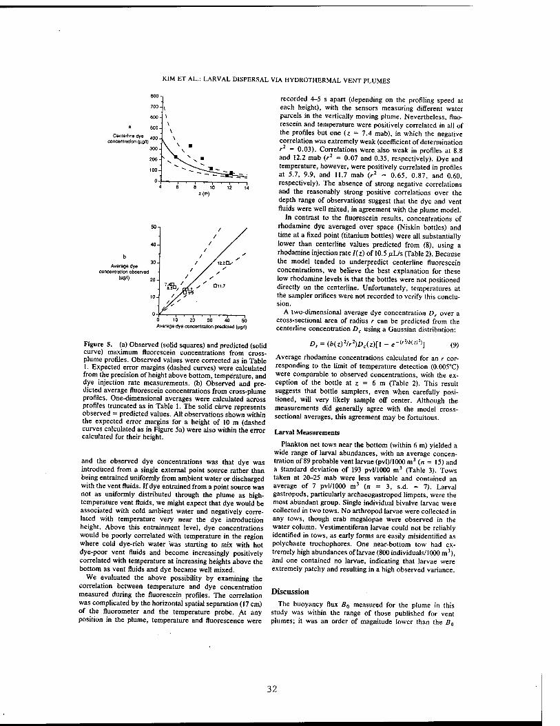
KIM ET AL.: LARVAL DISPERSAL VIA HYDROTHERMAL VENT PLUMES
Centerline dye 40n
concentration (ng/t)
300
*<m)
Average dye concentration observed
(HTJ/1)
0 10 20 30 40 SO Average dye concentration predicted (pig/!)
Figure S. (a) Observed (solid squares) and predicted (solid curve) maximum fluorescein concentrations from cross- plume profiles. Observed values were corrected as in Table I. Expected error margins (dashed curves) were calculated from the precision of height above bottom, temperature, and dye injection rate measurements, (b) Observed and pre- dicted average fluorescein concentrations from cross-plume profiles. One-dimensional averages were calculated across profiles truncated as in Table 1. The solid curve represents observed = predicted values. All observations shown within the expected error margins for a height of 10 m (dashed curves calculated as in Figure 5a) were also within the error calculated for their height.
and the observed dye concentrations was that dye was introduced from a single external point source rather than being entrained uniformly from ambient water or discharged with the vent fluids. If dye entrained from a point source was not as uniformly distributed through the plume as high- temperature vent fluids, we might expect that dye would be associated with cold ambient water and negatively corre- lated with temperature very near the dye introduction height. Above this entrainment level, dye concentrations would be poorly correlated with temperature in the region where cold dye-rich water was starting to mix with hot dye-poor vent fluids and become increasingly positively correlated with temperature at increasing heights above the bottom as vent fluids and dye became well mixed.
We evaluated the above possibility by examining the correlation between temperature and dye concentration measured during the fluorescein profiles. The correlation was complicated by the horizontal spatial separation (17 cm) of the fluorometer and the temperature probe. At any position in the plume, temperature and fluorescence were
recorded 4-5 s apart (depending on the profiling speed at each height), with the sensors measuring different water parcels in the vertically moving plume. Nevertheless, fluo- rescein and temperature were positively correlated in all of the profiles but one (z = 7.4 mab), in which the negative correlation was extremely weak (coefficient of determination r2 = 0.03). Correlations were also weak in profiles at 8.8 and 12.2 mab (r2 = 0.07 and 0.35, respectively). Dye and temperature, however, were positively correlated in profiles at 5.7, 9.9, and 11.7 mab (r2 = 0.65, 0.87, and 0.60, respectively). The absence of strong negative correlations and the reasonably strong positive correlations over the depth range of observations suggest that the dye and vent fluids were well mixed, in agreement with the plume model.
In contrast to the fluorescein results, concentrations of rhodamine dye averaged over space (Niskin bottles) and time at a fixed point (titanium bottles) were all substantially lower than centerline values predicted from (8), using a rhodamine injection rate I(z) of 10.5 fiL/s (Table 2). Because the model tended to underpredict centerline fluorescein concentrations, we believe the best explanation for these low rhodamine levels is that the bottles were not positioned directly on the centerline. Unfortunately, temperatures at the sampler orifices were not recorded to verify this conclu- sion.
A two-dimensional average dye concentration Dr over a cross-sectional area of radius r can be predicted from the centerline concentration Dc using a Gaussian distribution:
£>, = (i(z)2/r2)Dc(z)[l - e-l'2,bU)2)] (9)
Average rhodamine concentrations calculated for an r cor- responding to the limit of temperature detection (0.005°C) were comparable to observed concentrations, with the ex- ception of the bottle at z = 6 m (Table 2). This result suggests that bottle samplers, even when carefully posi- tioned, will very likely sample off center. Although the measurements did generally agree with the model cross- sectional averages, this agreement may be fortuitous.
Larval Measurements
Plankton net tows near the bottom (within 6 m) yielded a wide range of larval abundances, with an average concen- tration of 89 probable vent larvae (pvl)/1000 m3 (n = 15) and a standard deviation of 193 pvl/1000 m3 (Table 3). Tows taken at 20-25 mab were less variable and contained an average of 7 pvl/1000 m3 (n = 3, s.d. = 7). Larval gastropods, particularly archaeogastropod limpets, were the most abundant group. Single individual bivalve larvae were collected in two tows. No arthropod larvae were collected in any tows, though crab megalopae were observed in the water column. Vestimentiferan larvae could not be reliably identified in tows, as early forms are easily misidentified as polychaete trochophores. One near-bottom tow had ex- tremely high abundances of larvae (800 individuals/1000 m3), and one contained no larvae, indicating that larvae were extremely patchy and resulting in a high observed variance.
Discussion
The buoyancy flux B0 measured for the plume in this study was within the range of those published for vent plumes; it was an order of magnitude lower than the B0
32

KIM ET AL.: LARVAL DISPERSAL VIA HYDROTHERMAL VENT PLUMES
obtained by Little et al. [1987] at 11 °N on the EPR and was at the low end of a range of values calculated by Bemis et al. [1993] for Juan de Fuca. An initial exit velocity calculated from this ß0 (from (2)) was 0.33 m/s. This is on the low end of most of the exit velocities reported in the literature (0.40 m/s reported by Lupton et al. [1985]; 0.63 m/s by Little et al. [1987]; and 0.7-2.4 m/s by Converse et al. [1984]). These comparisons indicate that although the plume in the present study was not particularly vigorous, it was not atypical.
The dilutions of the fluorescein and rhodamine dyes by the plume provide a way to evaluate whether the in situ fluorom- eter readings were affected by pressure. Fluorescein, with an initial concentration of 4.4 g/L, was diluted to a centerline concentration of 57 ^g/L at 11.7 mab, which is equivalent to an; average concentration of 21 /u.g/L over the cross-sectional area of the plume (equation (9); bounded by the distance at which expected temperature dropped below the level of detection). The resulting dilution ratio was 2.1 x 10⁵. Rhodamine, with an initial concentration of 7.5 parts per thousand, was diluted to 50 parts per billion at 11.0 mab, a 2.2 x 10⁵ ratio. The similarity between these dilution ratios supports the supposition that the in situ fluorometer pro- vided reliable measurements.
Several independent observations suggest that dye was entrained and diluted in the plume as expected from the model. Predicted average fluorescein dye concentrations were within a factor of 2 of observed levels, with no consistent bias of under- or overprediction of entrainment. Although maximum fluorescein concentrations were consis- tently higher than predicted, all but two were within mea- surement error. A positive correlation between dye concen- tration and temperature was observed in all but one profile, indicating that dye from an external point source was mixing with vent fluids within a few meters of the entrainment level. We believe that observed discrepancies in some of the profiles were not-unexpected consequences of limitations in our sampling procedures (i.e., instantaneous point sampling and inaccuracies in positioning sensor). The rhodamine concentrations were substantially lower than centerline val- ues predicted from the buoyancy flux and height off the bottom, as were values in the four lower fluorescein transects. We believe that these samples were taken off center, as positioning the sensors or samplers directly in the center of the plume was difficult, particularly in the lower 10 m. The difficulty in obtaining reliable centerline dye concentra- tions with bottle samplers serves as a caution for attempting to measure centerline larval abundances using similar samplers in the plume.
The observations that all the visible dye was entrained into the plume and that fluorescein dye and temperature were positively correlated at several locations in the plume sug- gest that it is reasonable to use centerline plume tempera- tures and external tracer concentrations to model fluxes of the tracer up to the lateral spreading level. If the tracer is a larva, then we have an additional task of evaluating whether it can be considered passive and neutrally buoyant. Direct measurements of sinking and swimming speeds for hydro- thermal vent larvae are lacking, but if we assume that they are similar to those of related shallow-water larvae, the sinking speeds should be within the range from 0.17 to 0.83 cm/s [Chia et al., 1984]. Vertical velocities in the rising plume are approximately 10 cm/s. This disparity implies that larvae of vent species can indeed be entrained and vertically
advected by hydrothermal plumes. Converse et al. [1984] calculate that fewer than 3% of particles with sinking speeds as high as 1.68 cm/s will fall out of a plume rising 250 m above the bottom. Thus most of the larvae should be carried to the top of the rising plume. Additional evidence for vertical larval transport comes from observations of even large, relatively heavy postmetamorphic juveniles of benthic species high in a plume over Juan de Fuca Ridge [Mullineaux et al., 1991].
To determine the flux of larvae reaching the top of the plume, we calculate the rise height of the plume (the height of the top of the lateral plume) zmax from the following [Morton et al., 1956]:
Zmax=5(iy7r)"4/v-
N = [(glp)(dpldz)y
(10)
(11)
where p is the density of the ambient seawater. The buoy- ancy frequency N = 1.6 x 10~4 s~' was calculated from observed conductivity-temperature-depth profiles. Using B0 = 3.61 x 10"5 m4/s3 from above, zmax was calculated to be 205 m. On the same cruise, a zraax of 240 m was observed over the same portion of the ridge by P. H. Wiebe (personal communication, 1992). The observed zmax was defined as the height at which the light attenuation anomaly, recorded by transmissometer, decreased to e~' of the maximum attenuation anomaly.
The larval flux at the top of the plume can be calculated from the known concentration of larvae outside the plume and the volume of ambient fluid entrained. We use a surface integral for entrainment through the conical plume surface 5 to calculate larval flux out of the top of the plume F0M:
j j LV dS, = f j LV dS0 + \\ LV dS,
Sz (12)
Here L is the larval concentration, 50 is the plume source surface, 5) is the approximately conical plume surface, and S2 is the circular plume surface at the base of the spreading level. We assume that no larvae are present in the source fluid. For a conical surface, // dSt = f2irb(z) dz, and the larval flux Fin into the plume between two levels z, and z2 is, for L constant between those two levels,
Fm = L\ 2irb{z)Ve dz (13)
Here Ve is the horizontal entrainment velocity at the plume edge and is [Turner, 1973]
Vt=yWc (14)
with the empirically determined entrainment coefficient y = 0.07 [Turner, 1973]. Using (2) and (14), (13) becomes
Fio = Z.27r/3yC,(B^3)(3/5)(z25/3 - z?'3) (15)
Like (2), this is valid only well below zmax. Assuming that the ambient larval concentration L is zero above z2 and below zi, FBM = Fin.
Mean larval abundance within 6 m of the bottom was 89 individuals/1000 m3. If we assume that larvae were entrained
33

KIM ET AL.: LARVAL DISPERSAL VIA HYDROTHERMAL VENT PLUMES
only from this region (z, = 0 m, z2 = 6 m), then 22 pvl/h, would enter the spreading level of the plume. This number is equivalent to an average concentration of 0.49 pvl/1000 m3
(following (8)) in the spreading portion of the plume. Larvae, however, were observed in plankton net tows above 6 m; net tows taken at 20-25 mab averaged 7 pvl/1000 m3. This result suggests that some benthic larvae were being entrained into the plume even at 25 m off the bottom. At the spreading level of the plume, entrainment from 20-25 mab results in a flux of 6 pvl/h, and a density of 0.13 pvl/1000 m3. If we interpolate larval abundances, assuming a linear relationship with height above bottom, we estimate a mean abundance of 47 pvl/1000 m3 between 6 and 20 mab. If we sum the larval flux into the plume below 25 m, Fout = Z Fin and the mean number of benthic larvae reaching the spreading level of the plume is 102 pvl/h, for a larval concentration in the spreading plume of 2.30 pvl/1000 m3.
For comparison, the maximum ambient larval concentra- tions observed were 800 individuals/1000 m3 within 6 m of the bottom and 14 individuals/1000 m3 between 20 and 25 m. Using the procedure described above, we calculate a maxi- mum flux of 836 pvl/h and a maximum density of 19.0 pvl/1000 m3 in the spreading plume. The order of magnitude difference between these values and the averages suggests that the larval supply to the spreading level may be ex- tremely patchy. Dense patches of larvae, if they remain coherent during entrainment and dispersal, may enhance recruitment success and colony establishment by ensuring the arrival of a critical number of reproductive colonists.
To determine whether these larval flux estimates can be generalized, we compared them to calculations using the larval abundances at 21°N on the East Pacific Rise reported by Berg and Van Dover [1987]. Using our conservative criterion for categorizing vent larvae (groups found solely or predominantly at vents), abundances of probable vent larvae (Calyptogena, Munidopsis, and Bythograea) in near-bottom tows at 21°N were similar to our average densities: an average of 103 larvae/1000 m3 (« = 6, s.d. = 69) within 14 m of the bottom. If the 21°N gastropods (which probably included some nonvent species) are included in the calcula- tions, the average is 296 larvae/1000 m3. Assuming a similar initial vent buoyancy flux and no larvae above 14 m, this abundance results in 104 (298 with gastropods) larvae/h entering the spreading level of the plume and a spreading- level concentration of 2.36 (6.77 with gastropods) larvae/ 1000 m3. The maximum flux rate of 858 larvae (including gastropods) per hour at the 21°N sites was comparable to our measurements at 9°N, as was the expected concentration in the lateral plume (19.5 larvae/1000 m3). Despite the similar- ity in overall numbers of vent larvae, the types of larvae found were very different at the two sites. These differences may be due in part to differences between the vent commu- nities in the two areas. Other sources of variability in larval supply, such as synchronized or seasonal spawning, also affect larval densities.
In general, these results predict that larval abundances in the spreading plume should be roughly 2 orders of magnitude lower than those in near-bottom waters and that fluxes from vent communities with similar reproductive output are likely to average on the order of 100 larvae/h, with an upper bound close to 1000 larvae/h. The similarity in abundance of vent larvae to that at 21°N suggests that these predictions may be generalizable along the East Pacific Rise. The calculated
larval fluxes and lateral-plume abundances are only weakly sensitive to the estimate of B0 OSo'3; compare (15)); varying B0 over the range reported from vents along the East Pacific Rise [Converse er al., 1984; Little et al., 1987] and the Juan de Fuca Ridge [Bemis et al., 1993] changes the estimates only slightly.
These estimates of vertical larval flux and larval abun- dance in a spreading plume provide a "null model" for comparison with future observations. Deviations of ob- served larval abundances in the laterally spreading plume from those expected from near-bottom abundances and plume flux estimates may reveal important larval behaviors or physical processes. For instance, it is possible that larval behaviors such as chemotaxis to vent-specific chemicals could inhibit dispersion in the lateral plume and result in anomalously high concentrations of larvae near the source of the spreading plume. Alternatively, recent work with plume mechanics has suggested that geostrophic vortex flows may be forced by high-temperature venting [e.g., Speer, 1989; Helfrich and Battisti, 1991] and may concentrate larvae in patches [Mullineaux et al., 1991]. Even in the absence of plume-forced vortices, studies of deposition from plumes predict the existence of a specific down-current area that will consistently receive high densities of particles [Ghoneim et al., 1993]. Either of these physical mechanisms could pro- vide large numbers of recruits to a limited area, enhancing colonization and species survival probabilities.
The present study shows that a standard plume model appears to describe the dynamics of an external tracer sufficiently well to use the model for predicting larval en- trainment and vertical fluxes. Calculations of expected larval fluxes at sites near 9° and 21°N along the EPR demonstrate that a substantial number of vent larvae should be entrained into hydrothermal plumes and transported to a level several hundred meters above the seafloor. These predictions can be tested with field observations and provide a first step toward estimating vertical larval fluxes on large geographical scales. The results presented here emphasize the need to consider horizontal currents not only near the seafloor but also at the level of the lateral plume in order to understand dispersal of vent larvae in deep-ocean flows. Because of strong vertical shears near midocean ridges, trajectories of vent larvae dispersing in the lateral plume may be considerably different from the paths of larvae remaining near the seafloor. The next step in understanding how far and in what direction larvae can disperse and successfully colonize remote vent habitats is to combine estimated larval trajectories based on horizontal and vertical flows with information on larval sinking speeds, swimming behaviors, and life spans.
Acknowledgments. We are very grateful to L. Garland, C. Lewis, and P. Wiebe, who provided extensive support in all aspects of this project. We would like to thank R. Catenach, S. Gleason, R. Pawlowicz. and the crews of the Atlantis II and DSV Alvin. Aanderaa Instruments very generously loaned us an RCM8 current meter for the cruise. S. Little and three anonymous reviewers greatly improved the manuscript with their comments. This research was supported by NSF grant 9019575, WHOI Education, Ocean Ventures Fund, and Seaspace/Houston Underwater Club. This is contribution 8421 of the Woods Hole Oceanographic Institution.
References Baker. E. T.. Hydrothermal plume prospecting: Hydrographie and
geochemical techniques, in Gorda Ridge, edited by G. R. McMur- ray, pp. 155-167, Springer-Verlag, New York, 1990.
34

KIM ET AL.: LARVAL DISPERSAL VIA HYDROTHERMAL VENT PLUMES
Bemis, K. G., R. P. Von Herzen, and M. J.'Mottl, Geothermal heat flux from hydrothermal plumes on the Juan de Fuca Ridge, J. Geophys. Res., 98, 6351-6365, 1993.
Berg, C. J., and C. L. Van Dover, Benthopelagic macrozooplankton communities at and near deep-sea hydrothermal vents in the eastern Pacific Ocean and the Gulf of California, Deep Sea Res., 43, 379-401, 1987.
Cannon, G. A., D. J. Pashinski, and M. R. Lemon, Middepth flow near hydrothermal venting sites on the southern Juan de Fuca ridge, J. Geophys. Res., 96, 12,815-12,831, 1991.
Chen, C. J., and W. Rodi, Vertical turbulent buoyant jets: A review of experimental data, in Science and Applications of Heal and Mass Transfer, Series V4, edited by D. B. Spalding, 83 pp., Pergamon, New York, 1980.
Chia, F. S., J. Buckland-Nicks, and C. M. Young, Locomotion of marine invertebrate larvae: A review. Can. J. Zool., 62, 1205- 1222, 1984.
Converse, D. R., H. D. Holland, and J. M. Edmond, Flow rates in the axial hot springs of the East Pacific Rise (21°N): Implications for the heat budget and the formation of massive sulfide deposits, Earth Planet. Sei. Lett., 69, 159-175, 1984.
Fretter, V., and M. C. Pilkington, Prosobranchia, in Fiches d"Iden- tification du Zooplancton, edited by J. H. Fräser and V. K. Hansen, Conseil International pour l'Exploration de la Mer, sheets 129-132, pp. 1-26, Charlottenlund, Denmark, 1970.
Ghoneim, A. F., X. Zhang, and O. M. Knio, Dispersion and deposition of smoke plumes' generated from massive fires, J. Hazard. Mater., 33, 275-282, 1993.
Gustaffson, R. G., D. T. J. Littlewood, and R. A. Lutz, Gastropod egg capsules and their contents from deep-sea hydrothermal vent environments, Biol. Bull., 180, 34-55, 1991.
Haymon, R. M., R. A. Koski, and C. Sinclair, Fossils of hydrother- mal vent worms from Cretaceous sulfide ores of the Samail Ophiolite, Oman, Science, 223, 1407-1409, 1984.
Haymon, R. M., D. J. Fomari, M. H. Edwards, S. Carbotte, D. Wright, and K. C. MacDonald, Hydrothermal vent distribution along the East Pacific Rise Crest (9°09'-54'N) and its relationship to magmatic and tectonic processes on fast-spreading mid-ocean ridges, Earth Planet. Sei. Lett., 104, 513-534, 1991.
Helfrich, K. R., and T. M. Battisti, Experiments on baroclinic vortex shedding from hydrothermal plumes, J. Geophys. Res., 96, 12,511-12,518, 1991.
Little, S. A., K. D. Stolzenbach, and R. P. Von Herzen, Measure- ments of plume flow from a hydrothermal vent field, J. Geophys. Res., 92, 2587-2596, 1987.
Lupton, J. E., J. R. Delany, H. P. Johnson, and M. K. Tivey, Entrapment and vertical transport of deep-ocean water by buoy- ant hydrothermal plumes, Nature, 316, 621-623, 1985.
Lutz, R. A., Dispersal of organisms at deep-sea hydrothermal vents: A review, Oceanol. Ada, special volume, 23-29, 1988.
Lutz, R. A., D. Jablonski, and R. D. Turner, Larval dispersal and development at deep-sea hydrothermal vents, Science, 226, 1451- 1453, 1984.
MacDonald, K. C, Mid-ocean ridges: Fine scale tectonic, volcanic
and hydrothermal processes within the plate boundary zone, Anna. Rev. Earth Planet. Sei., 10. 155-190, 1982.
Middleton, J. H., and R. E. Thomson, Modeling the rise of hydrothermal plumes. Can. Tech. Rep. Hydrogr. Ocean Sei., 69, 14 pp., Dep. of Fish, and Oceans, Inst. of Ocean Sei., Sydney, B. C, 1986.
Mileikovsky, S. A., Speed of active movement of pelagic larvae of marine bottom invertebrates and their ability to regulate their vertical position, Mar. Biol, 23, 11-17, 1973.
Morton, B. R„ G. Taylor, F. R. S. Turner, and J. S. Turner, Turbulent gravitational convection from maintained and instanta- neous sources, Proc. R. Soc. Lond. Ser. A, 234, 1-23, 1956.
Mullineaux, L. S., P. H. Wiebe, and E. T. Baker, Hydrothermal vent plumes: Larval highways in the deep sea?, Oceanus, 34, 64-68, 1991.
Roberts, P. J. W., and W. H. Snyder, Merging buoyant jets in a stratified crossflow, U.S. Environ. Prot. Agency Res. Dev. Rep., EPA-2, 1987.
Rouse, H., C. S. Yih, and H. W. Humphreys, Gravitational con- vection from a boundary source, Tellus, 4, 201-210, 1952.
Scheltema, R. S., On dispersal and planktonic larvae of benthic invertebrates: An eclectic overview and summary of problems, Bull. Mar. Sei., 39, 290-322, 1986.
Speer, K. G., A forced baroclinic vortex around a hydrothermal plume, Geophys. Res. Leu., 16, 461^»64, 1989.
Speer, K. G., and P. A. Rona, A model of an Atlantic and Pacific hydrothermal plume, J. Geophys. Res., 94, 6213-6220, 1989.
Tesch, J. J., Pteropoda Thecosomata, in Fiches d'Identification du Zooplancton, edited by J. H. Fräser and V. K. Hansen, Conseil International pour l'Exploration de la Mer, sheet 8, pp. 1-6, Charlottenlund, Denmark, 1947.
Thiriot-Quievreux, C, Heteropoda, Oceanogr. Mar. Biol., II, 237-261, 1973.
Tunnicliffe, V., The biology of hydrothermal vents: Ecology and evolution, Oceanogr. Mar. Biol., 29, 319-407, 1991.
Turner, J. S., Buoyancy Effects in Fluids, 368 pp., Cambridge University Press, New York, 1973.
Turner, R. D., R. A. Lutz, and D. Jablonski, Modes of molluscan larval development at deep-sea-hydrothermal vents, Biol. Soc. Wash. Bull., 6, 167-184, 1985.
Van Dover, C. L„ C. J. Berg, and R. D. Turner, Recruitment of marine invertebrates to hard substrates at deep-sea hydrothermal vents on the East Pacific Rise and Galapagos spreading center, Deep Sea Res., 35, 1833-1849, 1988.
Von Damm, K. L., J. M. Edmond, B. Grant, and C. I. Measures, Chemistry of submarine hydrothermal solutions at 21°N, East Pacific Rise, Geochim. Cosmochim. Ada, 49, 2197-2220, 1985.
Wishner, K. F., The biomass of deep-sea benthopelagic plankton, Deep Sea Res., 27, 203-216, 1980.
K. R. Helfrich, S. L. Kim, and L. S. Mullineaux, Woods Hole Oceanographic Institution, Woods Hole, MA 02543:
(Received,July 1, 1993; revised January 18, 1994; accepted March 9, 1994.)
35

Chapter 3
Identification of Archaeogastropod Larvae
from a Hydrothermal Vent Community
INTRODUCTION
Since hydrothermal vent habitats in the deep sea are ephemeral and spatially
disjunct, the question of how vent species disperse is an interesting issue. Most common
vent species have planktonic larvae able to disperse in the water column, though the adults
usually are sessile and endemic to a vent environment. For ecological studies which
include larval stages, identification of larvae to the species level is necessary. However,
the morphological characteristics used for species identifications among adults may not be
the same as those for larvae. While larval characteristics may be sufficient to distinguish
between species, they may not be adequate for the identification of species if such
characters are not retained into adulthood.
At hydrothermal vents along the East Pacific Rise, the most abundant taxa are
vestimentiferans, polychaetes, bivalves, and gastropods. Larvae of Vestimentifera have
not been found in the water column, though their developmental sequence can be inferred
from that of related pogonophorans (Southward 1988). Polychaete larvae are difficult to
identify to species, because their morphological characteristics often do not reliably
correspond to those of adults. Most polychaete larvae collected near vents are in early
developmental stages (trochophore or early metatrochophore) and are too small to identify
past family level. In such soft-bodied taxa, a species-specific genetic probe or some other
technique for matching larvae to adults will be necessary to make larval identifications.
In most molluscs, the larval shell is retained on the apex of the adult shell.
Ornamentation on the surface of the shells is often detailed and usually species-specific,
and shell shape and details of aperture and hinge are also useful morphological
characteristics. The initial shell laid down by a larva is known as the protoconch I in
36

gastropods, or prodissoconch I in bivalves. Larvae of both gastropods and bivalves can be
identified by close examination of such a larval shell, and by comparisons with the
prodissoconch I or protoconch I of known adult species. Published micrographs of vent
adults often show details of the larval shell (i.e. Turner et al. 1985, McLean 1988, McLean
1989a, b, Waren and Bouchet 1989, McLean 1993, Waren and Bouchet 1993). Thus,
some species can be identified by comparison of the larval shell with the protoconch or
prodissoconch of the adult (Mullineaux et al. 1995).
Other techniques for larval identification are to rear captured larvae from the
plankton to an identifiable juvenile or adult stage (Scheltema 1971), or to spawn adults,
fertilize eggs and then raise the larvae in the laboratory. Such techniques require rearing
conditions and the appropriate food for larval development, and a source of spawning
adults or larvae. The environment at vents, such as high pressure and variable oxygen and
sulfide concentrations, may be difficult to replicate in the laboratory, so that maintaining
adults or raising larvae is not easy and has not yet been accomplished. The methods of
larval collection result in specimens that may be damaged by mechanical trauma from the
nets or pumps used, and by differences in pressure and temperature experienced between
the point of collection and the surface. While it may be possible to construct a sampling
device that would collect larvae gently and bring them to the surface at in situ pressure and
temperature, the relatively low abundances of larvae (20-100/1000 m3; Kim et al. 1994,
Mullineaux et al. 1995) would require processing large volumes of water. Such a collector
would be expensive and challenging to construct.
Molecular techniques offer another method for identification of larvae to species. A
genetic probe can be created that complements a known species-specific DNA sequence. If
the probe binds to DNA from a larvae, the species is identified. Progress has been made
on sequencing portions of the genome of some species found at vents (Tillier et al. 1994,
R. C. Vrijenhoek, pers. com.). Work is advancing steadily on this technique, but it has
not yet reached a usable form for vent species. A simpler alternative is to resolve
37

recognizable banding patterns from adult DNA using restriction enzymes and compare this
to the banding pattern obtained from larvae (R. A. Feldman, pers. com.). This method is
quick because no sequencing is necessary, but less likely to be successful for all species
because enzymes can detect a change only within their recognition sites. Both techniques
require equivalent knowledge of related species, in order to define characteristics (sequence
or banding pattern) that are species-specific. Since genetic techniques could potentially be
useful for all species (cf. Grassle and Grassle 1976, Olson et al. 1991, Tunnicliffe et al.
1993), not just those with hard parts retained by the adults, and because they may require
less individual manipulation of specimens, they will ultimately be very effective
approaches.
Each of the techniques available for larval identification has limitations.
Morphological techniques rely on the retention of larval characters by adults; even in
gastropods the protoconch may be deciduous or may become covered by the teleoconch or
adult shell as it develops, and distinguishing between within-species and between-species
variability requires multiple samples of both adults and larvae. Raising larvae of deep-sea
species is technically difficult and awaits the development of appropriate sampling and
culturing techniques. Genetic methods are expensive, time consuming, and labor
intensive, but have potential for easy processing of large samples by using visually tagged,
species-specific probes (Delong et al. 1989) and may be especially useful for identification
of morphologically similar species (Grassle and Grassle 1976).
Currently, only morphological identification of larvae of vent species is a reliable
technique. It is tempting to assume that because a larval type is common near vents, that it
must be a species indigenous to a vent environment, but this is not always true. Species
identification is required to define the distributions of larvae of vent species and necessary
to answer ecological questions concerning the dispersal patterns of species restricted to
vents. Identifications can be made among some gastropod species by morphological
comparison of the larval shell with the protoconch of an identifiable adult. In this chapter I
38

demonstrate the use of scanning electron microscopy (SEM) as an effective technique for
species-specific identification of vent gastropod larvae.
MATERIALS AND METHODS
Larvae were collected during research cruises aboard the RV Atlantis H/DSV Alvin
in December 1991 and November 1994. The series of Alvin submersible dives were
conducted in the Venture Hydrothermal Fields along the East Pacific Rise, a fast spreading
center located from 9°09'N to 9°54'N and 104°14'W to 104°18'W that has been well-
mapped by Haymon et al. (1991). The area was volcanically active as evidenced by recent
lava flows. The ridge crest is at -2500 m depth, with a small axial graben <200 m wide
and <100 m deep. Both black smokers and shimmering flows are common.
Plankton samples were taken around the vents and in and around the plume of
hydrothermal fluid rising from the vents, using nets of 64 urn mesh for capturing smaller
larvae. Near-bottom sampling from Alvin was conducted with a 3-net deep-tow system
(Gowing and Wishner 1986) or with a 5-bin plankton pump. Pump samples were taken
within the caldera close to hydrothermal structures and communities (i.e. chimneys, diffuse
vents, mussel beds). Deep-tows were taken within or just outside the axial caldera.
Sampling from the ship was done with an 18-net MOCNESS (Multiple Opening Closing
Net Environmental Sensing System, Wiebe et al. 1985), and tows were taken in and
around the neutrally buoyant plume.
On return to the surface, samples were immediately rinsed from the nets with
seawater and chilled. Care was taken to avoid contamination by surface plankton, by
rinsing nets from the outside and using filtered seawater when it was necessary to rinse
inside the nets. Deep-tow and pump samples were quickly examined under a dissecting
microscope (at 50x) for larvae, and preserved in buffered formalin within 4 hours of
recovery. Samples were later transferred to 70% ethanol.
39

All samples were later sorted at 50x under a Wild M5A dissecting microscope.
Larvae were divided into visually distinguishable groups, and gastropods were drawn with
a camera lucida. These images were less than ideal, and attempts were made to improve
them with camera images taken with a phototube and Olympus OM4 and Ektachrome 400
film. However, it was impossible to distinguish species-specific characteristics at this
magnification. I then tried to distinguish shell ornamentation under a compound scope, and
though some characteristics were discernible, even at 400x the characteristics were not
distinct. These improved images were archived using a digital camera system, consisting
of a Nikon 8008S, a Kodak DCS200, a Macintosh Quadra 840AV, and Photoshop v. 2.5.
Further magnification and higher contrast required the use of a scanning electron
microscope (SEM) to visualize the very fine species-specific ornamentation. Individuals
that were indistinguishable under even high magnification on a light microscope became
easily differentiated by their surface structure under SEM. Preparation of the specimens for
scanning was a difficult and time-consuming process, and could not have been completed
without the patience and skill of Alan Pooley at Rutgers University. Individual larvae were
oriented apex up and mounted with 3M 850 silver tape on stubs, air dried and sputter
coated with gold/palladium. When samples appeared encrusted under the dissecting scope,
they were treated with a 50% bleach solution to remove surface deposits. Though a few
specimens were lost or crushed in the preparation process, excellent images of most were
obtained. The SEM was an AMRAY 18301, in the lab of Richard Lutz at Rutgers
University. Settings were 10 kV, with a 10-12 mm working distance. Buildup of charge
in the SEM can cause size measurements or magnifications to be systematically erroneous,
so a correction factor to determine the exact sizes of the larvae was obtained from the
relative size of a spherical bead under the SEM and under a calibrated dissecting
microscope.
These protoconch micrographs were grouped and compared with published
micrographs of adults. Where possible, the original adult specimens were located from the
40
collection at Rutgers University and re-imaged so that magnifications and orientations of
larval shells matched those of protoconchs on adults as closely as possible. The groupings
of larvae done under the light microscope were subdivided under the SEM to the lowest
taxonomic level possible. One of the initial groupings made under the light microscope
contained at least eleven species in five families, though all were within one order.
These species identifications were examined by Philippe Bouchet, an expert in deep
sea gastropod taxonomy at the Museum national d'Histoire naturelle in Paris, who
confirmed the identifications of vent species, and identified non-vent specimens, some to
genus.
RESULTS
The characteristics that distinguished the gastropod veliger larvae of vent species
from those not indigenous to the vent environment were general size and shape of the shell.
The vent gastropods found were all of the superorder Archaeogastropoda. The
protoconchs were small, single-whorled, dextrally coiled (though this may be difficult to
determine even with SEM), and exhibited distinctive sculpting patterns. Other gastropod
larvae found were usually multi-whorled, or if single-whorled, lacked surface
ornamentation.
The characteristics used to distinguish species within superorder
Archaeogastropoda were protoconch size, the shape of the aperture, and protoconch
ornamentation, which included striation or lines (cf. Figure 1 A), reticulation or webbing
(cf. Figure 3A), and punctation or indentations (cf. Figure 5A). The three types of
sculpturing formed distinct categories that simplified comparisons with the many published
protoconch types, though family designations did not always fall within such groupings.
In some cases, protoconch morphologies for all members of a taxon were not known. In
such instances, the genus name or a species name within the genus was assigned based on
41

the known distribution of adults along the East Pacific Rise. A question mark preceding a
taxon indicates uncertainty.
Within the family Peltospiridae, four species were found. All have sculpting of
parallel striations, but exhibit distinct differences that allow species-level identification.
Rhynchopelta concentrica (2 larval specimens) has a large protoconch (285-290 (im),
fourteen broad, gradually raised ridges meeting in a curve at the apex, and a shelf at the
axis of coiling (Figure 1A-C). Peltospira ?operculata (6 larval specimens) has a moderate-
sized protoconch (200-230 jxm), nineteen steep-sided ridges meeting at a point, and no
shelf (Figure 2D-F). Species identification for Peltospira is not certain because two
congeners remain whose protoconch morphologies are unknown (McLean 1989a, Waren
and Bouchet 1989), and one is also found at 9°N. The third species was Lirapex granularis
(1 larval specimen), with a medium-sized protoconch, 230 jim, and approximately ten
parallel grooves as well as pustulose ornamentation near the suture (Figure 1G-I).
Four larval types were recovered with reticulate sculpturing on the protoconch.
Two were similar, both 175-190 fim, with faint reticulation and a straight aperture (Figure
2A-B). Slight differences include a flare at the aperture of one, and sculpting that does not
extend to the shell edge in the other, though this difference could be due to preservation in
formalin. These two forms (4 larval specimens) were assigned to the genus
?Melanodrymia, in family Peltospiridae, since the larval shells were each very similar to the
protoconch of Melanodrymia aurantiaca (Figure 2C-D). An undescribed species of
Melanodrymia has been reported from the 9-10° N site (R. G. Gustafson, pers. com.).
The two other specimens with reticulate protoconchs were identified as Cyathermia
natacoides in family Cyathermidae, and Neomphalus fretterae, in the family Neomphalidae.
Cyathermia natacoides (2 larval specimens) has a 240-255 |im protoconch, strong reticulate
sculpting and a wavy margin (Figure 3A-C), while N. fretterae (1 larval specimen) has a
maximum dimension of 260 |im, fine reticulation and a very sinuous aperture (Figure 3D-
F). Examples of protoconchs for all confamilial species found between Galapagos and
42

Guaymas were available, and thus clearly defined species-specific sculpting patterns for
these two larval types were established (McLean 1981, Waren and Bouchet 1989).
Five species had punctate protoconchs. In family Gorgoleptidae, a species of
Gorgoleptis was identified (1 larval specimen). The protoconch morphology of only one
of three congeners was available (Figure 3H,I); the protoconch of the species that is found
at 9°N has not been described or imaged. The punctate larval shell is small (180 um), has
deep, dense indentations, with faint striations near the aperture and a very sinuous margin
(Figure 3G).
Clypeosectus delectus (1 larval specimen), in the family Clypeosectidae, is also
small (175 |im), with coarse, closely spaced punctate sculpting, organized into distinct
parallel striations, and a straight aperture (Figure 3J-L). No congeneric Clypeosectus have
been found on the East Pacific Rise, but one is present on Juan de Fuca Ridge for which
protoconch morphology is undescribed (McLean 1989b).
Among the remaining punctate larvae, three distinct morphotypes were found that
correspond with the protoconchs of three known species. The differences between the
larval shells were subtle, but as they match differences in the adults, they have been
tentatively identified as Lepetodrilus ?elevatus galriftensis (10 larval specimens),
Lepetodrilus ?elevatus elevatus (9 larval specimens), and Lepetodrilus ?ovalis (7 larval
specimens). All are small, ranging from 165 to 210 |im. One larval morphotype has two
sizes of small indentations (average diameters 0.6 and 1.3 |im) that are organized into a line
following the shell curve (Figure 4A), as does the protoconch of L. elevatus galriftensis
(Figure 4D, G). The second morphotype has evenly sized, large indentations (average
diameter 1.8 Jim) with a similar line (Figure 4B), matching the protoconch of L. elevatus
elevatus (Figure 4E, H), and the third morphotype has evenly-sized large indentations
(average diameter 2.3 (im), with no linear organization (Figure 4C), like the protoconch of
L. ovalis (Figure 4F, I).
43

Figure 1 Larvae and juveniles in family Peltospiridae. Scale bars are 50 urn for all shells except C (400 urn), F (200 urn) and I (300 um). A - Rhynchopelta concentrica larva from 9°50'N, EPR, 5 meters above bottom
(mab) B - Rhynchopelta concentrica protoconch from 21°N, EPR C - Rhynchopelta concentrica juvenile shell from 21°N, EPR D - Peltospira ?operculata larva from 9°50'N, EPR, 5 mab E - Peltospira operculata protoconch from 21°N, EPR F - Peltospira operculata juvenile shell from 21°N, EPR G - Lirapex granularis larva from 9°50'N, EPR, 5 mab H - Lirapex granularis protoconch from 21°N, EPR I - Lirapex granularis juvenile shell from 21°N, EPR
44

45

Figure 2 Larval ?Melanodrymia spp. and juvenile Melanodrymia aurantiaca . Scale bars are 50 (im for all shells except D (300 \im). A - ?Melanodrymia sp. larva 1 from 9°50'N, EPR, 5 mab B - ?Melanodrymia sp. larva 2 from 9°50'N, EPR, 100 mab C - Melanodrymia aurantiaca protoconch from 21°N, EPR D - Melanodrymia aurantiaca adult from 21°N, EPR
46

47

Figure 3 Larval and juvenile archaeogastropods. Scale bars are 50 fim for all shells except C (400 um), F (1000 \im), I (400 \un) and L (200 um). A - Cyathermia natacoides larva from 9°50'N, EPR, 5 mab B - Cyathermia natacoides protoconch from 21°N, EPR C - Cyathermia natacoides juvenile shell from 21°N, EPR D - Neomphalus fretterae larva from 9°50'N, EPR, 5 mab E - Neomphalus fretterae protoconch from 21°N, EPR F - Neomphalus fretterae juvenile shell from 21°N, EPR G - Gorgoleptis sp. larva from 9°50'N on EPR, 5 mab H - Gorgoleptis emarginatus protoconch from 21°N, EPR I - Gorgoleptis emarginatus juvenile shell from 21°N, EPR J - Clypeosectus delectus larva from 9°50'N, EPR, 5 mab K - Clypeosectus delectus protoconch from 21°N, EPR L - Clypeosectus delectus juvenile shell from 21°N, EPR
48

47

Figure 3 Larval and juvenile archaeogastropods. Scale bars are 50 urn for all shells except C (400 |lm), F (1000 um), I (400 um) and L (200 |im). A - Cyathermia natacoides larva from 9°50'N, EPR, 5 mab B - Cyathermia natacoides protoconch from 21°N, EPR C - Cyathermia natacoides juvenile shell from 21°N, EPR D - Neomphalus fretterae larva from 9°50'N, EPR, 5 mab E - Neomphalus fretterae protoconch from 21°N, EPR F - Neomphalus fretterae juvenile shell from 21 °N, EPR G - Gorgoleptis sp. larva from 9°50'N on EPR, 5 mab H - Gorgoleptis emarginatus protoconch from 21°N, EPR I - Gorgoleptis emarginatus juvenile shell from 21°N, EPR J - Clypeosectus delectus larva from 9°50'N, EPR, 5 mab K - Clypeosectus delectus protoconch from 21°N, EPR L - Clypeosectus delectus juvenile shell from 21°N, EPR
48

49

j -i Q™1P bars are 50 urn for all shells except for G Figure 4 Larval and juvenile ^(«*^^cate bars are \i
S (200 pm), H (100 urn) and I (200 ^ • pR 5 mab
A - Lepetodrilus ? elevatus «^^SSfeim Galapagos B - Lepetodrilus elevatus galnftensis V^™*™™™m Galapagos C- Lepetodrilus elevatus galnftensis juvenilev8^™ ^ab D -Lepetodrilus ?elevatus elevatus larva from 9 50NW
g:ffeS£ ÄÄ I - Lepetodrilus ovalis juvenile shell from Galapagos
50

51

Because of the limited number of adult specimens imaged, uncertainty remains as to
whether the slight morphological differences between these protoconchs actually delineated
species. Even adult characteristics which distinguish L. elevatus galriftensis from L.
elevatus elevatus are small, and possibly are due simply to differences in habitat.
Lepetodrilus elevatus galriftensis is a geographic subspecies limited to the Galapagos
vents and not found along the East Pacific Rise. Distinctive differences in larval shells and
their similarity with protoconchs on adults suggest that larvae of both subspecies were
present at 9°N.
Eleven species in six families have been identified from larvae collected near 9-10°N
on the East Pacific Rise. All the other larval gastropod specimens collected were from non-
vent species. Holoplanktonic pelagic forms were of the order Thecosomata (pteropods) or
the family Carinariidae (heteropods) (examples in Figure 5A-B). One pelagic heteropod
genus in the past has been tentatively identified as veliger larvae of a vent gastropod species
(Turner et al. 1985). The distinctive veligers of two species of the heteropod Atlanta
(Thiriot-Quievreux 1973) are commonly found in the plankton (Figure 5C-F). Because of
past confusion, the evidently common occurrence of these species near vents, and the
distinctive nature of the shells, images are included here.
Two larval types from non-vent but benthic species were found; an unidentified
eulimid (Figure 6A-B) and ?Laeviphitus sp. (Figure 6C-D). These groups are easily
distinguished from the vent archaeogastropods by the lack of sculpting on the protoconch
and development of multiple whorls while still planktonic.
DISCUSSION
I have found that characteristics of protoconch morphology can be used to identify most
gastropod larvae to species. For some of the specimens identified here, geographic
distributions of adults were used to determine the most probable species identification
within genera. This was necessary when protoconchs of related species were unknown.
52

Using information on geographical distribution to assist in identifications assumes that (1)
the species list from the site is complete, and (2) that larvae of species present at any given
site are more likely to be found than larvae of species from other sites. Though the area
from 9-10°N has been visited many times, sampling for gastropods in vent habitat is
demanding and all collections have been incidental to collections of large animals or
geological specimens. Thus, though the species list is as complete as that for any vent site,
it is not definitive, and the assumption that all species from a site are known remains
questionable. In cases where adult distribution has been used to designate species,
alternative identifications should be explored.
Among the three obvious sculpting patterns (striated, reticulated, and punctate),
specimens with striated protoconchs are easiest to identify because morphological
differences are clearly defined. All species with striated protoconchs belong to the family
Peltospiridae (Table 1). Lirapex granularis has a congener, L. humata, but the protoconchs
of the two species are distinctly different (Waren and Bouchet 1989). One possible
congener of Rhynchopelta concentrica , (R? nux; Okutani et al. 1993) has been described,
but its the protoconch morphology is unknown. Since R? nux is found only near Japan I
feel confident that the larvae found at 9°N is R. concentrica.
Two species of Peltospira, P. operculata and P. delicata, are found at 9°N on the
East Pacific Rise. The protoconch of P. operculata appears identical to the larval shells
found at 9°N. Adult specimens of P. delicata tend to lose their protoconchs (McLean
1989a), though the scar left on the adult shell indicates that the protoconchs are the same
size as the larval shells found in the present study. A third congener, P. lamellifera, has
been found along the East Pacific Rise, though not at 9°N. Peltospira lamellifera is very
rare, and the only scanning electron micrographs available show a specimen with mineral
deposits obscuring the protoconch. One other species, Nodopelta subnoda, has a
protoconch that appears similar to the larval specimens, but the correspondence in
morphology is not as exact as that of P. operculata. Because P. operculata has been found
53

Figure 5 Representative examples of pelagic pteropods and heteropods. Scale bars are 50 |im for all shells except for B (25 (im). A - Pteropod (order Thecosomata) from 9°50'N, EPR, 5 mab B - Heteropod (family Carinariidae) from 9°50'N, EPR, 5 mab C - Side view of Atlanta sp. 1 larva from 9°50'N, EPR, 5 mab D - Top view of Atlanta sp. 1 larva from 9°50'N, EPR, 5 mab E - Side view of Atlanta sp. 2 larva from 9°50'N, EPR, 5 mab F - Top view of Atlanta sp. 2 larva from 9°50'N, EPR, 5 mab
54
55

Figure 6 Larvae of non-vent, benthic species. Scale bars are 50 Jim for all shells. A - Top view of eulimid larva from 9°50' N, EPR, 200 mab B - Side view of eulimid larva from 9°50' N, EPR, 200 mab C - Side view of ?Laeviphitus larva from 9°50'N, EPR, 5 mab D - Top view of ?Laeviphitus larva from 9°50'N, EPR, 5 mab
56

57

o ;
(D 4—» a o
a c .2 1"* 0) -
o o .3
cd PH
4)
4-» o
1 e (D 4-»
G Ü
3 O IS
I
PH o «3 £
5
(D .O ON 00 ON CO 1—' ON 3 ON CvS i—i <D „
ON ON HJ ON 00 00 o 00
o o ON ON S ON
ON ON #> ■*->
ON ON 1) <D »r> <D i—1 *—H XI XI oo J3
^ ^ o o x _o ON O O ^ ""> 3 3 ON ON i—i 3 ON oo 00 o O 00 OO O ON ON ON PQ PH ON ON 15 PQ <—i >—i >—i V—1 r—1
cLea
n cL
ean
cLea
n =3 =3 C
J3 cLea
n cL
ean <D
s- <D
E 3 H
s 1
SSS £ £S£ £ PA ^ PH PH w W
OH (F Pi £ p< PH ON PH ON PH
ffl . W ffl
iF Pi 2 PH P* PH o
PH PH < o
ONWÜ W W ON W Ü ON
o & 0J.H 15 g _ra to in g
■B "2 5 On CM <U 52 o c o o "a g, &"g IS « .*» O S g^Cn CM E5
-C bO CM >, <D 'S
<a o ö ü (U « ^^ s Cfl C/3 C
tr-1 tr*.^ *« fc- "-<
fli ^ Ja <+H 3 <^ T3 MH <H a) b <C
CO
58

ON 00 ON
<D JS o 3 O
pq
3
co ON ON
00 00 OO 00 oo oo 00 oo ON ON ON ON
c S c s cd cd cd cd D <L> u a)
o o o o
»n >o in vT oo oo oo oo ON ON ON ON T-' ,_H '—' <—' oo co
cd cd cd cd ON ON
U Ü U <D c ui cd
oo oo ON T—H
s cd D
o
oo ON 1—1 oo ^-! OO
cd ON ■4—» *""*
n cd
ID U U U (j U !U <D E£ E E^J Ed O Ü
£ E^^SS 3
"d- ON 00 OO ON ON
C cd
£ o CO j^ 3 ON O O ON r-1 m ~£
=3 ON ON ON" ON ON
c l-c
OO 00 00 00 00 ON ON ON ON r^ ON '—i r—< i—i i—i CO .
ON ON tJ
J3
cd 4~» <D CL>
X! „ o O O O ■!rl <-> cd >o 3 3 3 3 a 3 ON oo O O O O
3ffl cd oo
ON PQ mm m CT\ 0\
~- <% =3=3 =3 pq^ 00 ^
2 3 cd s 3 3 3 =3 8 cd
-t—» <D <D <D <D 3 <Q
<D
E 3
l-C cd cd cd
**
War
19
93
C- cd (v-j
cLea
M
cL
v-f «n vf oo J2
a,W
98
5,
chet
2 lO H 00 oo oo -oo
ON ON ON ON o cd n-t n-( iri ^oS ""' 1—1 r—1 _| '-' 3 ON ON ^ 3 ON ON ON CO 00 T-H
ON . OO • , ; t_^ _: ° oo 00 ■ O 00 OO OO ON ON cd cd cd cd pq ON ON cd PQ ON ON ON ON ""! ^ a <D 0> <D o=3 3 c U^ c 3
r—(
c cd a) cd s-< i-i V.
Tur
ner
War
en cd cd s-i ^H cd cd cd Cd *r> I-,
<D
o
<D c S-H
3 H T
urne
T
urne
McL
e M
cLe
Tur
ne
War
er
McL
e M
cLe;
M
cLe;
L
utze
T
urne
:
P4 p-, pq
öS Pi PH pq
ÜONS&NÜW
OS CL, w
WON
CL, tfi
•4 < Ü
P4 OH pq
o ON
ptS PL, pq
P-1 CM pq
P4 P4 ^ ^04 P4 P4 04 P4 P4 P4 P4 04 -£P4
pqpqoNONpqpqgqwpqpqpqgqpqoNpq
-a D 3 .3 %-» 3 o o
59

at 9°N, and the protoconch is so similar to the larval shells, these larvae were identified as
P. ?operculata.
Specimens with reticulate sculpting on their larval shell were all identified within the
superfamily Neomphaloidea, but in different families. Cyathermia natacoides, family
Cyathermidae, and Neomphalusfretterae, family Neomphalidae, are closely related but
have distinctly different and unique protoconch ornamentation (Figure 3). The specimens
identified as ?Melanodrymia spp., family Peltospiridae, are similar to the protoconchs of
several species in the same family, or within the superfamily. All these species differ
slightly in the degree of reticulation and aperture shape, and have different adult
distributions. Melanodrymia aurantiaca, in family Peltospiridae, has light webbing over
most of the protoconch, and occurs on the East Pacific Rise though not at 9°N. Leptogyra
inflata, also in family Peltospiridae, has light webbing over the apical part of the
protoconch and a curved aperture, but has been found only in the Western Pacific.
Symmetromphalus regularis, in superfamily Neomphaloidea, has light webbing over the
entire protoconch, and has been found only in the Western Pacific. Two species have
incomplete webbing over part of the protoconch; Planorbidella planispira (family
Peltospiridae) has reticulation reduced to fragments and is found along the East Pacific Rise
though not at 9°N, and Lacunoides exquisitus (superfamily Neomphaloidea) has been
found at Galapagos but not along the East Pacific Rise. Two species with heavy
reticulation are Pachydermis laevis (family Peltospiridae) and Solutigyra reticulata; they
were recently moved to family Skenidae from Peltospiridae (Waren and Bouchet 1993).
Pachydermis laevis has a bulbous aperture and is found along the East Pacific Rise but not
at 9°N; S. reticulata, with reticulation over half the protoconch, has been found at 9°N.
Morphological features of the larval shells match Melanodrymia aurantiaca protoconchs
most closely, though they are not identical. A further justification for identifying the
specimens as ?Melanodrymia spp. is the presence of an undescribed species of
Melanodrymia at the 9°N site.
60

The possibility remains that a larval morphogroup might match an undescribed
protoconch more closely than any of the known protoconch morphologies. Echinopelta
fistulosa, Hirtopelta hirta, Nodopelta heminoda, Peltospira delicata and P. lamellifera, in
family Peltospiridae, are found along the East Pacific Rise and have undescribed
protoconchs. These species probably have protoconchs with ridged ornamentation,
indicated by the protoconch morphologies of the most closely related species (Ctenopelta
porifera, N. subnoda, P. operculata), though other species in the same family have
reticulate sculpting. Without knowing the protoconch morphologies of every species,
some potential for mis-identification of larvae exists.
Larvae with punctate protoconch morphology are the most difficult to identify, as
differences in sculpting are slight. Two species of Clypeosectus, namely C. delectus and
C. curvus, have been described (McLean 1989b). The protoconchs of C. delectus and
larval shells were indistinguishable (Figure 4D-F), and C. delectus adults are found at 9°N,
so I identified these specimens as ?C delectus. It is unlikely that the larvae are
Clypeosectus curvus, as this species has been found only in the northeast Pacific. The
protoconch of C. curvus is undescribed, as protoconchs of all imaged adult specimens have
been obscured by mineral deposits. The only other species with a similar protoconch
morphology is Sutilizone theca, family Scissurellidae, which resembles, but does not
match, the shell morphology of the larvae in question.
Gorgoleptis emarginatus, G. spiralis and G. patulus are the three known species of
Gorgoleptis. Both G. spiralis and G. patulus are rare, and protoconchs of known
specimens are obscured by mineral deposits (McLean 1988). Gorgoleptis spiralis has
been found at 9°N, G. emarginatus elsewhere along the East Pacific Rise, and G. patulus
only at Galapagos. The match between larval shells and protoconchs of G. emarginatus
was close, but not exact. The presence of the rarer G. spiralis adults at the 9°N site
suggests that the larvae were G. spiralis, though the possibility that they belong to one or
both of the other species cannot be completely excluded.
61

Five species in the genus Lepetodrilus are found along the East Pacific Rise
(McLean 1988, 1993). Four of these, Lepetodrilus ovalis, L. elevatus, L. cristatus and L.
pustulosus, are found at 9°N. Additional site-specific species are found at Guaymas (L.
guaymasensis), off Japan (L. japonicus), in the western Pacific (L. schrolli), and two in
the northeast Pacific (L. fucensis and L. corrugatus). A separate sub-species (L. elevatus
galriftensis) is found at Galapagos hydrothermal communities. The larval shells divided
clearly into three groups, though the characteristics differentiating them were slight.
Difficulties arose when trying to assign each of these morphogroups to species, because
protoconch morphologies are only known for L. elevatus elevatus , L. elevatus galriftensis
and L. ovalis. The matches between larval shells and protoconchs on adults are good, but
without examining several adult specimens, some uncertainty remains as to whether the
characteristics seen are truly species-specific, or are merely variable between individuals.
As protoconch morphologies of more lepetodrilid species become known, these
identifications should be reevaluated.
Of the 11 species of larvae found, seven were also found as adults in the same area.
All opportunistic collections of adult gastropods at the 9°N site have yielded a total of 15
species. The collection of adults was necessarily limited to those species which live closely
with larger animals such as the tubeworm Riftia and the mussel Bathymodiolus. Thus,
species which are primarily found on rock surfaces rather than biogenic ones are
underrepresented. The eight species found as adults but not as larvae may have non-
planktonic larval stages (Morton 1968), reproduce periodically, or simply be too rare as
larvae to be found in the net samples.
Four of the larval species found were not represented in the collections of adults,
but these species are found elsewhere, at 13 or 21 °N along the East Pacific Rise, or at
Galapagos. It is unclear whether this observation means simply that sampling of the adults
is incomplete at 9°N, or that larvae from other sites are reaching 9°N.
62

Larvae from other areas of active venting are probably present at 9°N. Known
species distributions span ridge systems over 3000 km, and there are less than 350 km
between sites at 9°N and at 13°N. Advection in near-bottom currents could transport larvae
over the distance between 9 and 13°N. If currents average 5 cm/s along the ridge crest
(Cannon et al. 1991), it would take 12 weeks to transport between the two sites; it is
feasible that larvae remain planktonic for this length of time.
Both the morphological comparisons as described here, and molecular genetic
techniques, allow identification of individual larvae. Large samples, which are difficult to
obtain, are not necessary, and even rare species can be identified. Knowledge about
congeneric and confamilial species is required for definitive identifications. Such a
database has not been built for genetic analysis but one is currently available and usable,
though incomplete, for shell morphology of vent archaeogastropods. A limitation of the
morphological technique is that it requires much handling of small individual protoconchs,
and a degree of skill with the scanning electron microscope. Genetic techniques require
less precise manipulation, and could decrease handling time and losses significantly.
Morphologically-based identification is useful only for species which retain identifiable
larval characteristics into adulthood. However, at the present time it is the only technique
available for identification of molluscan larvae of vent species. The ability to identify vent
larvae reliably is a major step towards defining larval distribution patterns and mechanisms
at hydrothermal vents.
LITERATURE CITED
Cannon, G. A., D. J. Pashinski and M. R. Lemon. 1991. Middepth flow near hydrothermal venting sites on the southern Juan de Fuca ridge. Journal of Geophysical Research 96:12,815-12,831.
Delong, E., G. S. Wickham and N. R. Pace 1989. Phylogenetic stains: ribosomal RNA- based probes for the identification of single cells. Science 243: 1360-1363.
Gowing, M. M. and K. F. Wishner. 1986. Trophic relationships of deep-sea calanoid copepods from the benthic boundary layer of the Santa Catalina Basin, California. Deep-Sea Research 33:939-961.
Grassle, J. P. and J. F. Grassle. 1976. Sibling species in the marine pollution indicator Capitella. (Polychaeta). Science 192:567-569.
63

Haymon, R. M., D. J. Fornari, M. H. Edwards, S. Carbotte, D. Wright, and K. C. Macdonald. 1991. Hydrothermal vent distribution along the East Pacific Rise crest (9°09'-54'N) and its relationship to magmatic and tectonic processes on fast-spreading mid-ocean ridges. Earth and Planetary Science Letters 104: 513-534.
Hickman, C. S. 1984. A new Archaeogastropod (Rhipidoglossa, Trochacea) from hydrothermal vents on the East Pacific Rise. Zoological Scripta 13(1): 19-25.
Kim, S. L., L. S. Mullineaux, and K. R. Helfrich. 1994. Larval dispersal via entrainment into hydrothermal vent plumes. Journal of Geophysical Research 99(C6): 12655- 12665.
McLean, J. H. 1981. The Galapagos rift limpet Neomphalus: Relevance to understanding the evolution of a major Paleozoic-Mesozoic radiation. Malacologia 21(1-2): 291-336.
McLean, J. H. 1988. New archaeogastropod limpets from hydrothermal vents: superfamily Lepetodrilacea I. Systematic descriptions. Philosophical Transactions of the Royal Society London B 319: 1-32.
McLean, J. H. 1989a. New archaeogastropod limpets from hydrothermal vents: new family Peltospiridae, new superfamily Peltospiracea. Zoologica Scripta 18(1): 49-66.
McLean, J. H. 1989b. New slit-limpets (Scissurellacea and Fissurellacea) from hydrothermal vents. Part 1. Systematic descriptions and comparisons based on shell and radular characteristics. Contributions in Science, Natural History Museum of Los Angeles County 407: 1-29.
McLean, J. H. 1993. New species and records if Lepetodrilus (Vetigastropoda: Lepetodrilidae) from hydrothermal vents. Veliger 36(1): 27-35.
Morton, J. E. 1968. Molluscs. London, Hutchinson and Co. Mullineaux, L. S., P. H. Wiebe, and E. T. Baker. 1995. Larvae of benthic invertebrates in
hydrothermal vent plumes over Juan de Fuca Ridge. Marine Biology 122:585-596. Okutani, T., K. Fujikura, and T. Sasaki. 1993. New taxa and new distribution records of
deepsea gastropods collected from or near the chemosynthetic communities in the Japanese waters. Bulletin of the National Science Museum series A (Zoology) 19(4): 123-143.
Olson, R. R., J. A. Runstadler, T. D. Kocher. 1991. Whose larvae? Nature 351:357-358. Scheltema, R. S. 1971. Larval dispersal as a means of genetic exchange between
geographically separated populations of shallow-water benthic marine gastropods. Biological Bulletin 140:284-322.
Southward, E. C. 1988. Development of the gut and segmentation of newly settled stages of Ridgeia (Vestimentifera): Implications for relationship between Vestimentifera and Pogonophora. Journal of the Marine Biological Association of the United Kingdom 68: 465-487.
Thiriot-Quievreux, C. 1973. Heteropoda. Oceanography and Marine Biology Annual Review 11:237-261.
Tillier, S., M. Masselot, J. Guerdoux, and A. Tillier. 1994. Monophyly of major gastropod taxa tested from partial 28S-rRNA sequences, with emphasis on Euthyneura and hot-vent limpets Peltospiroidea. Nautilus 108 (Suppl. 2): 122-140.
Turner, R. D., R. A. Lutz, and D. Jablonski. 1985. Modes of molluscan larval development at deep-sea hydrothermal vents. Biological Society of Washington Bulletin 6: 167-184.
Tunnicliffe, V., D. Desbruyeres, D. Jollivet, and L. Laubier. 1993. Systematic and ecological characteristics of Paralvinella sulfinicola Desbruyeres and Laubier, a new polychaete (family Alvinellidae) from northeast Pacific hydrothermal vents. Canadian Journal of Zoology 71:286-297.
Waren, A. and P. Bouchet. 1989. New gastropods from east Pacific hydrothermal vents. Zoologica Scripta 18(1): 67-102.
Waren, A. and P. Bouchet. 1993. New records, species, genera, and a new family of gastropods from hydrothermal vents and hydrocarbon seeps. Zoologica Scripta 22(1): 1-90.
64

Wiebe, P. H., A. W. Morten, A. M. Bradley, J. E. Craddock, T. J. Cowles, V. A. Barber, R. H. Backus and G. R. Flierl. 1985. New developments in the MOCNESS, an apparatus for sampling Zooplankton and micronekton. Marine Biology 87:313-323.
65

Chapter 4
A Cellular Automata Model of Larval Dispersal and
Population Persistence in Hydrothermal Vent Habitats
INTRODUCTION
Hydrothermal vents are distributed as archipelagos of habitat distinct from the
surrounding deep sea environment. At vents, seawater is chemically altered and heated by
passing through geothermally active regions beneath the seafloor. The chemicals in this
hydrothermal fluid are utilized by chemosynthetic organisms which reproduce prolifically
near vents, and these bacteria form a large food resource that is unusual in the deep sea. To
take advantage of this abundant food supply, vent organisms must be able to tolerate the
unusual vent chemistry which would poison unadapted animals. Dependence on this food
source comes at a price: vent organisms are unable to survive away from hydrothermal
areas. Thus, organisms that inhabit vent habitat are found only at vents, though large-scale
distributions for a few species extend along ridge crests across ocean basins (Tunnicliffe
1991). Because of the patchy arrangement of vents, animals must have a mechanism of
transport between isolated sites to maintain species continuity. This chapter examines how
the persistence of a population in a patchy habitat, such as hydrothermal vents, is effected
by larval abundance and survival, and by dispersal mechanisms.
Hydrothermal vents occur predominantly along mid-ocean ridge crests, where the
plates of the earth's crust are spreading apart. The distribution of vents (both spatial and
temporal) appears correlated with the spreading rate of the ridge crest system. At fast
spreading ridges (-15 cm/yr), the axial summit caldera, where most of the hydrothermal
activity takes place, is very narrow and linear, and vents average a few tens of meters apart
(Fornari and Embley 1995). The ridge crest is underlain by a melt lens that provides a heat
source for hydrothermal flows through shallow fissures, and the fluid flow pathways are
frequently reorganized by volcanic activity. Vents can appear anywhere along the ridge
66

crest, with an overall pattern of geological succession where individual vents are active for
100 years out of a 1000 year cycle of general activity along the ridge segment overlying a
single magma chamber (Haymon et al. 1991). Along slower spreading ridges (~3 cm/yr)
the axial summit caldera is wider, and vents are tens of kilometers apart, with a less linear
overall distribution. Lateral offsets in the ridge crest are more closely spaced, and volcanic
activity is infrequent. Venting occurs periodically at faults whose locations are stable, and
the geological cycle follows a 1000 year active, 4000 year inactive pattern (Macdonald
1985, Humphris 1995). At slow spreading ridges, sites of venting are tectonically
constrained, rather than volcanically controlled as they are at fast spreading ridges.
Differences in habitat distributions may interact with the dispersal capabilities of
vent species, possibly accounting for some of the differences in species composition
between communities at fast- and slow-spreading ridges. At slow spreading ridges the
dominant species in terms of biomass are bresilid shrimps (Van Dover et al. 1988), which
have the potential to disperse as adults. Biomass dominants at faster spreading ridges
include clams, mussels, and vestimentiferan tube worms, all of which are sessile and have
extremely limited mobility as adults.
Most marine invertebrates have a planktonic larval stage that is well suited for
dispersal in the water column. Many factors impact the dispersal potential of a larva,
including larval lifespan, physiological tolerances, and feeding capabilities. These life-
history characteristics can be studied directly in shallow nearshore, intertidal, or near-
surface species, by field and laboratory measurements. For organisms from hydrothermal
vent ecosystems, such approaches are difficult to execute. Larvae of vent organisms have
been difficult to raise in the lab, though recently C. M. Young (Young et al. in press) has
had limited success with vestimentiferan species. Direct observations of dispersal paths are
difficult, for the larvae of vent organisms are small and occur in low densities. However,
as larvae do not swim rapidly, they probably act as passive particles and track the water
flow near vents. Flow is dominated by two patterns: near-bottom currents which are
67

topographically constrained to flow principally along the ridge crest (Cannon et al. 1991,
pers. obs.), and buoyant plumes of hot water that rise from vents, entraining ambient water
until positive buoyancy is lost and the neutral plume spreads laterally with the currents a
few hundred meters above the sea floor (Lupton et al. 1985). Either or both of these larval
dispersal pathways may be important to the establishment and maintenance of vent
populations (Mullineaux and France 1994). It is possible that a dispersive adult, which can
survive transport over long distances, is required for species persistence along ridge crests
where vents are widely spaced.
Additional factors that influence colonization success and species distributions are
settling cues (such as presence of conspecific adults), survival to reproduction, population
maturation time, and size of the reproductive population. No explicit studies on these
factors have been done for species from hydrothermal vents, though research on
recruitment is currently being conducted (Mullineaux et al. in press). For now, we cannot
examine the influence of these factors directly, though we can estimate values from the
literature on known related species.
The colonization of new habitat patches and the evolutionary persistence of endemic
species are important, fundamental processes in ecology. Patchy habitat distributions are
common and are becoming more so as human activities continue to alter ecosystems.
Species persistence in any isolated habitat, from oceanic island chains to undisturbed
rainforest remaining after slash and burn agriculture, requires efficient colonization and
species maintenance processes. These processes are particularly interesting at vents
because the habitat is ephemeral, on the order of years to decades, so rapid dispersal is vital
to the survival of the species.
Much remains unknown about dispersal and colonization processes, and species
persistence and distributions at hydrothermal vents. We need to know fecundities,
spawning patterns, larval mortalities and whether these are temporally or spatially
dependent, larval lifespans and what factors limit these (i.e. feeding ability, metabolic rate),
68
and larval behavior patterns. We need precise information on currents and flow patterns
near vents, over time scales equivalent to larval lifespans. And we need more extensive
mapping of habitat and species distributions over large spatial scales. Then, we can begin
to answer directly questions such as: How far do larvae travel and what dispersal
pathways do they follow? How quickly do new vent habitats become colonized, and is this
process dependent on the distance to the nearest vent community? How do the spatial and
temporal variation of vents and the reproduction and larval ecology of vent species interact
to influence species distributions and persistence?
The research tools ecologists can use include observation, field experimentation,
laboratory studies, and mathematical modeling. Because of limited access and equipment
constraints in the deep sea, and the extreme habitat at vents, observation, experimentation
and laboratory work can be very difficult with hydrothermal vent organisms. Mathematical
modeling is not subject to the same limitations, though it is an abstraction of a natural
ecosystem. Just as we control variables in the lab and field to simplify the system of
interest, pose hypothesis and perform experiments, we can design and execute experiments
within a modeling framework to help identify important biological, physical and geological
processes. Insights gleaned from models are uniquely helpful when one or more of the
parameters is beyond experimental control, for example, when the spatial scale is too large
for easy manipulation (Bradbury et al. 1990, Jeltsch and Wissel 1992). Models are useful
in determining the key parameters in an ecosystem, and the expanded understanding of
community dynamics is particularly valuable for research at hydrothermal vents, where
field work is difficult, expensive and very time-constrained. Modeling cannot replace field
and laboratory work, but it is a valuable adjunct to research in an ecosystem when empirical
data are limited.
If we examine the distribution of single vent species, or even of vent communities,
we find a group of subpopulations, geographically isolated but connected by migration.
This type of spatially discontinuous but genetically connected distribution is called a
69

metapopulation (Lande and Barrowclough 1990). Metapopulations can be mathematically
modeled by cellular automata, a spatially explicit type of model that can incorporate the
discontinuities present in hydrothermal vent systems. Inclusion of spatial coordinates and
temporal variability in the model is necessary to mimic important characteristics of a
spatially structured system like vents, and precludes using models which neglect patchiness
(cf. May 1973).
In cellular automata, the state of the population, as well as time and space, are
divided into discrete units (Caswell and Etter 1992, Durrett and Levin 1994). The model
uses a map of equally-sized cells or patches, each of which may be in one of several states.
With each time step, the state of a cell may change, depending on the states of its
neighboring cells and the rules that govern the model. The neighborhood of a cell is
defined as the area within which cells affect each other. The transition rules of the model
are formulated to incorporate all the ecological variables that might influence neighboring
cells' states.
Cellular automata have advantages over other types of ecological models, in which
space, time, or population density are continuous, in the simplicity of their solutions
(Caswell and Etter 1992). In reaction-diffusion models, all parameters are continuous and
approximate spatiotemporal interactions reasonably, but their solution is computationally
unwieldy. Transition rules that govern cellular automata are simple and facilitate
determination of the key factors influencing the results. However, the results of cellular
automata are less precise than those of reaction-diffusion models, because in making all the
variables discrete, cellular automata become blind to processes occurring on scales finer
than the discrete units of the model.
Cellular automata have been used to study systems in which spatial patterns are a
distinctive feature. Early studies of ecological systems assumed spatial homogeneity as a
simplification, but ecologists now recognize the importance of habitat heterogeneity (Pickett
and Cadenasso 1995). Initially, models of patchy habitats included habitat proportions,
70

though they were not spatially explicit; in cellular automata specific information about
habitat locations is integral to the model (Hanski 1994). When habitat distributions are
distinctive, spatial structure cannot be ignored. Examples of areas where cellular automata
have been used include conservation biology, to determine the best management strategies
for the remaining subpopulations of a threatened species (Hanski 1994); pest control, for
pesticide use and management of outbreaks (Bradbury et al. 1990, Sherratt and Jepson
1993); in studies of larval dispersal (Etter and Caswell 1994); and in theoretical studies on
the effects of pattern on population dynamics (Silvertown et al. 1992, Colosanti and Grime
1993, Molofsky 1994).
The cellular automaton model is an abstraction, so the model runs test abstractions
of direct ecological questions. The questions addressed in this chapter, using a cellular
automata model, are:
A. What are the effects on metapopulation persistence of dispersal in near-bottom versus
above-bottom flows, or in diffusive versus advective regimes?
B. What effect does crustal spreading rate, and hence vent ephemerality and distribution,
have on metapopulation persistence?
C. What are the effects of larval mortality, population size, and population time to maturity
on metapopulation persistence?
MATERIALS AND METHODS
The Model
The cellular automaton model used here was designed to represent dispersal
between discrete patches of suitable habitat, where the patches are scattered and ephemeral
as is found for hydrothermal vent habitat. The transition rules simulate processes that
occur at vents: opening of new vents and cessation of existing venting, and local and
global dispersal of larvae. The original code was written by Ron Etter in THINK Pascal on
71

a Macintosh computer; I have modified the original code to adapt the model for vent
ecosystems (code available on request from the author).
This model is organized on a 256 x 256 grid of square cells. The top and bottom
boundaries are absorbing; larvae that disperse past these edges are lost from the simulation.
The side boundaries are periodic; larvae that disperse past a side edge re-enter the
simulation at the opposite side. This arrangement mimics an elongate, linear habitat
distribution, such as vents along a ridge crest. Each cell can be in one of four states:
uninhabitable (no hydrothermal habitat in the cell), habitable but unoccupied (vent present
in the cell), occupied (by reproductively immature individuals around a vent), or producing
larvae (a vent population of reproductive adults). A local neighborhood of 9 cells is
defined (Figure 1), where producing neighbors influence the likelihood of colonization
occurring in the central cell. The central cell can also be influenced by a global
neighborhood consisting of all the other cells in the simulation.
1 2 3
4 5 6
7 8 9
Figure 1. The local neighborhood of 9 cells in the cellular automaton. Cell 5 is the central cell; the states of the other cells influence the state of cell 5 in the following time step.
Three basic transition rules control the change in state of a cell at each time step:
one defines disturbance, i.e. the change from inhospitable habitat to hospitable (Pn) and
visa versa (Pd), one defines the probability that an occupied cell will begin producing larvae
(Pr), and one defines the colonization probability (C) for a given cell (Table 1, Figure 2).
72

State at t
State at t + 1 Unsuitable Suitable Occupied Producing
Unsuitable 1-Pn Pd Pd Pd
Suitable Pn (1-Pd)*(l-C) 0 0
Occupied 0 c (1-Pd)*(l-Pr) 0
Producing 0 0 Pr 1-Pd
Table 1. Transition rules for the cellular automaton model. A cell in a given state at time t has the given probability of moving into each other state at time t+1.
1-Pn 1-Pd
(1-Pd)*(l-C) (1-Pd)*(l-Pr)
Figure 2. Transition pathways for the cellular automaton model.
The first rule, on disturbance rate, abstracts the spreading rate of a ridge crest.
Since vent distribution and longevity appear to be related to spreading rate (Fornari and
Embley 1995), these geological factors are incorporated in this rule. The probability of
73

disturbance is based on the geological cycle underlying vent distribution along the ridge
crest, which has a period of active venting, tv, and an inactive period, tj. With a model
timestep t, and one vent per cell, the probability Pn that a new vent appears in a cell is
p-=r (1)
and the probability of the existing vent in a cell ceasing to be active, Pj, is
P- = f (2)
These disturbance probabilities assume that vents are independent of each other. It is likely
that neighboring vents actually have some influence on each other, depending on the
distance between vents, because a single melt zone supplies heat to all vents along a ridge
segment, and the plumbing system of subsurface hydrothermal fluid flow is
interconnected. However, it is unclear exactly what, if any, relationship there is between
individual vents, so at our present state of knowledge the simplified assumption of
independence is justified.
The second transition rule represents the time for a population to become
reproductively mature after it is established. The probability that an occupied cell begins
producing larvae depends on the organism maturation time relative to the model timestep.
For these simulations, the probability that an occupied cell becomes producing, Pr, was set
to 1; any cell that is colonized starts producing larvae in the next timestep. Simulations
were also run for the case where the populations were immediately reproductive. This
simplification allows straightforward examination of simple hypotheses about larval
transport; its inclusion keeps the model flexible enough to later examine the effects of
population maturation time.
74

The third transition rule, which describes colonization, depends on the number of
larvae getting to a new vent site and includes local and global terms that represent dispersal
and mortality. The local neighborhood is the immediately surrounding 8 cells, and the
global neighborhood is all the other cells in the model. In the local neighborhood, the
number of cells which are actively producing larvae is defined as nL, and the local
frequency of cells producing larvae, FL, is
FL = ^ (3)
In the global neighborhood, XIQ is the total number of producing cells. The map comprises
65536 cells, and the global frequency of producing cells, FG, is
65535 FG = T^b (4)
The local and global dispersal components can be thought of as representing near-
bottom and plume-level dispersal respectively, or alternatively, diffusive and advective
dispersal. Larvae may reach a new site via near-bottom flows, or through entrainment into
the buoyant plume and transport at the spreading level a few hundred meters off the
seafloor. Both diffusion and advection occur at both heights above the bottom. In near-
bottom flows, velocities are small and so dispersal distances are relatively short; this can be
represented in the model by local dispersal. Also, where larvae are moving close to the
seafloor, they are likely to settle out at the first hospitable habitat they encounter, which
would be a suitable neighboring cell in the model. Plume-level transport is represented by
global dispersal in the model, since once a larvae gets up into the plume it may travel long
distances before falling back to the seafloor. Flow velocities are typically higher at the
neutral buoyancy level than near bottom (Franks 1992), so horizontal dispersal distances in
the same time frame will be further in plume-level flows. Similarly, on a smaller scale
75

within near-bottom flows, diffusion can be thought of as transporting larvae locally and
advection globally. The canonical value for eddy diffusivity in the deep-sea is 1 cm2/s
(Toole et al. 1994), so in one hour a larvae might travel 0.3 m horizontally via diffusion.
Near-bottom current speeds average 0.05 m/s (Cannon et al. 1991, L. S. Mullineaux,
unpublished data), thus in the same period of time a larvae could be advected 180 m.
Two components of the colonization probability represent mortality; one affects
both types of dispersal, and another represents the increased risk of global dispersal. The
component affecting global and local dispersers equally is incorporated within a variable
that embodies the average time for suitable habitat to become colonized, regardless of
dispersal path. In the equation, it is assumed that population size controls larval supply,
and that the larger the supply, the shorter the time to colonization. Colonization probability
also incorporates predation and other factors influencing larval survival that decrease
colonization likelihood, potential settlement cues that increase colonization likelihood, and
the spatial separation of habitat patches. The separate mortality term for globally
transported larvae abstracts all the same mortality factors (predation, starvation, settlement
cues or missing them, and simply not landing at a vent) to mimic the potentially higher risk
experienced during global dispersal.
I assume that colonization is a random process and follows a Poisson distribution,
so that the probability of at least one larva colonizing a cell is 1 - e-M-, where [i is the average
number of larvae colonizing a cell. Let d be the average number of larvae that can reach the
central cell in one time step from "full" neighborhoods, that is, neighborhoods that contain
all producing cells. The importance of global dispersal relative to local dispersal is
represented by r (0 < r < 1), and s represents the survival of larvae subjected to an
additional mortality risk from global dispersal (0 < s < 1). Thus JLL is the number of larvae
that could reach the central cell (d) adjusted by the proportion of producing cells in the
neighborhoods (FG and FT_), and modified by the proportion of larvae in each dispersal
76

pathway (r) and the relative mortality (s). The probability that 1 or more larvae colonize a
cell is the colonization probability C, where
C = l-exp[-d(rsFG+(l-r)FL)] (5)
When r = 0, dispersal is entirely local, and when r = 1, dispersal is only global. The
relative survival, s, reflects the increased risk of global dispersal, which may be due to the
increased amount of time spent in the water column and extra exposure to predation and
other mortality hazards.
The cellular automaton map is initialized with the equilibrium percentage of the cells
unsuitable, Pd/(Pn+Pd), as derived below. The unsuitable cells were randomly distributed
across the map. All other cells were producing; assuming that all venting sites are
colonized rapidly (relative to the model timescale) after they appear agrees with field
observations (Lutz et al. 1994, Milligan and Tunnicliffe 1994, Mullineaux et al. in press).
The derivation for the stable proportion of cells in each state is as follows: A A Wv is the stable probability of a cell containing a vent and Wn is the stable probability that a
cell does not contain a vent (Figure 3). Since these are the only two possibilities,
Wv = 1 - Wn (6)
As before, Pn is the probability of a vent opening, and Pd is the probability of a vent A
closing. At equilibrium, Wn is constant, and equal to the number of non-venting cells that
remain non-venting plus the number of venting cells that cease activity,
so that
Wn = (l-Pn)Wn + Pd(l-Wn) (7)
Wn = Pd/(Pd + Pn) (8)
77

Inserting this solution into (6), the steady state proportion of cells containing vents is
Wv= Pn/(Pd + Pn) (9)
Pd
1-Pd Wv ) Wn ) 1-Pn
Figure 3. Schematic of stable distribution of vents. Wv is the stable probability of a cell containing a vent
A and Wn is the stable probability that a cell does not contain a vent. Pn is the probability of a vent opening, and Pj is the probability of a vent closing.
As the model executes, it examines each of the 65536 cells in turn. It checks
whether the cell is unsuitable, and if it is, whether a new vent opens up; if the probability of
a new vent appearing, Pn, is greater than a randomly generated (uniformly distributed)
number between 0 and 1, a new vent appears. If a cell is suitable, it becomes occupied if
the colonization probability C is greater than a random number between 0 and 1. If a cell is
occupied, it becomes producing in the next time step, assuming a population maturation
time of less than the model timestep. Lastly, cells that are suitable, occupied or producing
may become unsuitable if the disturbance probability Pd is greater than a random number
between 0 and 1. As these transition rules are performed for each cell in the landscape, the
changes in cell states are recorded but not executed until the end of the time step. Then, the
78

entire map changes at once, instead of changes propagating through the system within a
timestep. This procedure insures that inappropriate temporal scales are not introduced into
the model.
Parameter Values
Model simulations were run for various values of the parameters, set at realistic
values for testing specific questions. Some of the constraints on the model are set by the
geology of the mid-ocean ridge system. Disturbance probabilities, both of existing vents
closing and of new vents opening, are dependent on the geological cycle relative to the
model timestep. In the model, parameters Pn and Pd are set at 1 year/100 years and 1/900,
respectively, for a fast spreading ridge, or 1/1000 and 1/4000, respectively, for a slow
spreading ridge (time estimates of vent activity and inactivity from Lowell et al. 1995). The
implicit model timestep is the numerator of the disturbance probabilities, in this case, 1
year. If the timestep is much smaller, the disturbance probabilities become so low (i.e. if
the timestep was 0.1 year, at a slow spreading ridge Pd = 0.1 year/4000 years = 0.000025)
that the habitat changes relatively little and questions on habitat ephemerality cannot be
addressed effectively with the model. If the model timestep is set to be much greater than a
year, the mismatch between the order of magnitude of a realistic population maturation time
(0.3 to 20 years, see below) and the model timestep becomes extreme. If the population
maturation time is 1, it takes 1 model timestep (in this case, 1 year) for the population to
begin reproducing, and if it is 0, populations are immediately reproductive.
Cell size in the model corresponds to the spacing of individual vents. Average vent
spacing can range from 100 m on a fast spreading ridge to 65,000 m on slow spreading
ridges (Fornari and Embley 1995). The model is constrained to have only one vent per cell
to keep calculations of disturbance probabilities straightforward. In order to calculate the
probability that multiple vents in a cell would all close, rendering the cell unsuitable, the
model would need to keep track of the changing number of vents in each cell, in essence
79

examining a smaller spatial scale then the cell size. Additionally, the probability of a new
vent opening should depend on the number of vents already open in the cell, as well as on
the cell size, to preclude unrealistic situations like 100 vents in a cell 1 m across. It is
simpler to limit the number of vents per cell to 1, though this also constrains the cell size.
The steady state proportion of active cells on a fast spreading ridge is 10%, calculated from
(9), and to obtain a 100 m average vent spacing, the cell size must be 10 m. Substituting
the disturbance probabilities at a slow spreading ridge into (9), the equilibrium percentage
of cells containing vents is 20%, and 65 km is the average vent spacing, leading to a cell
size of 13 km.
The mean time it takes for a newly colonized vent population to begin producing
larvae is the inverse of the probability that an occupied cell begins producing larvae. We
have set Pr to 1, which sets the maturation time to a single timestep of the model.
Maturation time in nature may be as short as 4 months (Tunnicliffe 1991, Mullineaux et al.
in press) or as long as 20 years (Turekian et al. 1983, Lutz et al. 1985, Tunnicliffe 1991).
By eliminating the "occupied" state in some model runs, so that cells that are colonized
immediately become "producing", we were able to explore the dynamics when the
maturation time is less than the model timestep of 1 year.
The remaining term is colonization probability, a function that incorporates global
and local dispersal and mortality. Values for r, the proportion of dispersal that is global,
and s, the relative mortality of global dispersers, each cover the entire potential range from
0 to 1. A range of realistic values for d, the average number of colonizing larvae reaching a
cell, can be calculated from the expected time to colonization for a newly opened vent, E.
Since E = C1, we can substitute in (5) for C and solve for d, assuming that all neighbors
are producing (FL = 1, FG = 1), and there is no additional global mortality (s = 1),
d = -ln (10)
80

As E goes to infinity, d goes to 0, and as E goes to 1, d goes to infinity. From a plot of d
versus E (Figure 4), we selected intermediate values of E = 10, 2, and 1.1 timesteps for
initial model runs, which gives us d = 0.1054, 0.6931, and 2.3979 colonists.
3 4 5 6 7 8
E (expected timesteps to colonization)
Figure 4. The average number of colonizing larvae reaching a cell (d), as a function of the average time to colonization (E) varied from 1 to 10 timesteps. Values represent colonization from a neighborhood full of producing cells.
10
Simulations
Each model simulation was initialized with a map of randomly distributed
producing vent sites. Simulations were run until equilibrium was reached, when the
proportion of cells in each state had not changed over the last 500 timesteps (e.g. Figure 5).
At each timestep, the model outputs the number of cells in each state and their spatial
distribution.
Comparison of absolute equilibrium numbers of cells in different states between
model runs was not attempted because the absolute number of unsuitable cells depended on

6000
U4000
CD XI
3 z 2000
200 400 600 Model Timestep
800
Producing (d = 0.1054)
Suitable (d = 0.1054)
Producing (d = 0.6931)
Suitable (d = 0.6931)
Producing (d = 2.3979)
Suitable (d = 2.3979)
Figure 5. Representative time series of model results for low (d = 0.1054), moderate (d = 0.6931) and high (d = 2.3979) larval supplies. This example is from a
run with moderate global dispersal (r = 0.50) and moderate survival (s = 0.50). Heavy lines are producing cells, light lines are suitable cells.
82

the disturbance probabilities (Figure 2). The number of unsuitable cells stays steady within
a single simulation, representing the constant proportion of habitat which does not contain
hydrothermal vents, and initially each simulation contains only unsuitable and producing
cells. Thus, the proportions of cells in each state relative to the initial number of producing
cells were used for comparisons. The following two ratios were most informative for
comparisons between model runs: the final number of producing cells relative to the initial
number of producing cells, and the final number of occupied cells over the initial number of
producing cells. The ratio of producing cells is a measure of the suitable habitat that
contains mature communities, or proportion producing. The colonization efficiency is
represented by the proportion of suitable cells that are occupied but non-reproductive. The
proportion of newly colonized cells can only be calculated when "occupied" is a potential
cell state, and cells that are colonized become reproducing in one time step.
Five questions were addressed with the model, and evaluated in terms of the
proportion of producing cells at equilibrium and the proportion of occupied cells at
equilibrium.
1. What is the effect of varying the relative importance of local and global dispersal?
2. What is the effect of varying the relative mortality rates of global and local dispersal?
3. What is the effect of varying the average number of colonizing larvae?
4. How do the above effects interact with variations in habitat ephemerality?
5. What is the effect of immediate versus delayed population maturity?
These questions break down the general questions in the introduction into easily
investigated components. Question 1 addresses A: What are the effects on metapopulation
persistence of dispersal in near-bottom versus above-bottom flows, or in diffusive versus
advective regimes?; question 4 addresses B: What effect does crustal spreading rate, and
hence vent ephemerality and distribution, have on metapopulation persistence?; and
questions 2, 3 and 5 address C: What are the effects of larval mortality, population size,
83

and population time to maturity on metapopulation persistence? The pattern of model runs
outlined in Table 2 examined the specific questions 1-5 posed above.
Variables Values Question
r 0, 0.25, 0.50, 0.75, 1 1
s 0, 0.25, 0.50, 0.75, 1 2
d 0.1054, 0.6931, 2.3979 3
Pn/Pd 0.0011/0.01,0.00025/0.001 4
P_r 1, immediate* 5
Table 2. Parameter values for cellular automata model runs. Variable r represents the relative importance of global (r = 1) versus local (r = 0) dispersal; s represents survival of global dispersers (when r = 0, dispersal is local and the value of s is inconsequential); d represents the average number of colonizing larvae reaching a cell; Pn and P^ are the probabilities of a new vent opening and of an existing vent closing, respectively (covarying as both depend on timestep) for fast and slow spreading ridges; and Pr is the probability that a colonized cell becomes producing in the next timestep. *The effects of immediate production are investigated by eliminating "occupied" as a cell state. Question refers to the 5 questions that are being tested by the model.
RESULTS AND DISCUSSION
To accomplish all combinations of variables in Table 2, 252 simulations were run.
I show the results of representative model runs.
Local Dispersal
When dispersal is entirely local (r = 0), the population persists at a low level
(Figure 6). At model equilibrium, with high disturbance probabilities, less than 1% of the
number of initially producing cells contain communities that are producing larvae; at low
84

b.
bß C a 3
-a o l-H
OH
e o '6 o & o
OH
1 - r dz s =
- 2.3979 :0.25
A
0.8- - Pr = 1 ■
0.6- A A A
■
0.4- ■
0.2- ■
0" 1 —1 —) 1 1
'o 3
O \~ OH
e o '■S o O %-,
0-,
0 0.25 0.50 0.75 r
1T r = 0.5 s=l
0.8-1- Pr=l
0.6--
0.4-"
0.2
0 0.1054 0.6931
d 1 T
bß
1 0.81
| 0.6 f
o 0.41 a, o LH
CM 0.2--
d = 0.75 r = 0.6931 Pr=l
0 0.25 0.50 s
0.75
2.3979
A
1
■Pn/Pd = 0.0011/0.01 A Pn/Pd = 0.00025/0.001
■Pn/Pd = 0.0011/0.01 A Pn/Pd = 0.00025/0.001
■Pn/Pd = 0.0011/0.01 A Pn/Pd = 0.00025/0.001
Figure 6. Representative examples of the effects of disturbance probabilities on the proportion of producing cells at model equilibrium. At high disturbance probabilities, Pn/Pd = 0.0011/0.01; at low disturbance probabilities Pn/Pd = 0.00025/0.001.
a. versus global dispersal (r), at high larval supply (d = 2.3979) and low survival (s = 0.25).
b. versus larval supply (d), at moderate global dispersal (r = 0.50) and complete survival (s = 1).
c. versus survival (s), at high global dispersal (r = 0.75) and moderate larval supply (d = 0.6939).
85

disturbance probabilities, less than 15%. Without global dispersal, colonization is an
extremely rare event, despite the abundance of suitable habitat patches.
The small proportion of suitable habitat that contains producing communities at
model equilibrium when dispersal is only local is in contrast to what we have observed at
hydrothermal vent habitats, where nearly every vent found has had a mature community of
vent organisms around it. This suggests that in reality dispersal has at least some global
component. This could mean that advection or plume level dispersal are important to the
overall dispersal process at hydrothermal vents.
It is possible that at lower disturbance probabilities local dispersal is all that is
necessary to maintain populations. In the model, at low disturbance probabilities, the
proportion of productive habitats is up to 15% with only local dispersal. Though all vents
found at slow spreading ridges have had populations of vent organisms, this may be a
function of the low number of sites visited, and not an indication of the true proportion of
producing habitat. On the appropriate scale, dispersal between adjacent vents would need
to cover a distance of 65,000 m. For diffusion to transport larvae this far, using the
canonical eddy diffusivity value in the deep-sea of 1 cm2/s, larvae must live about 20
weeks, a fairly long time but not outside the range of reality. For advection to transport
larvae this far along the axis, with an average flow speed of 0.05 m/s, larvae would need to
survive 2 weeks to be transported between vents on a slow spreading ridge. Larval
lifespans of 2 or 20 weeks are both possible.
Population Persistence
The proportion of producing cells at model equilibrium is higher when disturbance
probabilities are low (Figure 7b). The proportion producing increases as the degree of
global dispersal (r) increases, the larval supply (d) increases, and the global survival (s)
increases. Global dispersal has the strongest influence on proportion producing; the
increase is proportionate when the disturbance probabilities are high and irregular when the
86

a.
Pn/Pd = 0.0011/0.01
11 r d = 0.6931 Pr=l
M0.8-
'o -o 0.6 - o
1-4
CL,
.2 °-4 ■ "-4—»
+
° s = 0
A s = 0.25
+ ♦ ♦ © A
• s = 0.50
♦ s = 0.75 O CL, 2 0.2-
0-,
+ ®
♦ A
Ä A n
+ s=l
n .
( ) 0.25 0.50 0.75 1
b.
Pn/Pd = 0.00025/0.001
1 - r d = 0.6931 •+ *
Pr = = 1 o
M0.8 J + e o
•a 0.6 - o s-, * Ä A
OH A O 0.4 - t; O &, 2 0.2-
OH
i I D a D D 0- —h- —i— 1 1
° S = 0
As = 0.25
• s = 0.50
♦s = 0.75
+ s = 1
0 0.25 0.50 0.75
Figure 7. Representative examples of the effects of survival (s) and global dispersal (r) on the proportion producing at model equilibrium, at constant larval supply (d = 0.6931).
a. at high disturbance probabilities (Pn/Pd = 0.0011/0.01). b. at low disturbance probabilites (Pn/Pd = 0.00025/0.001).
87

disturbance probabilities are low (Figure 7). At low disturbance probabilities, the
proportion of producing cells at equilibrium rises abruptly when 25% global dispersal is
added to the model, and when at least 25% of the larvae produced survive global dispersal
(except at 50% global dispersal and 50% survival). The suitable habitat becomes saturated
(i.e. all suitable habitat is producing) when 75% of the larvae produced are successfully
globally dispersed. Larval supply has a positive effect; increasing the supply increases the
final proportion of producing habitat (Figure 8). Increasing larval supply and increasing
global dispersal have similar effects on proportion producing when the disturbance
probability is high, and the effect is uniform across the range of larval supply values. The
influence of larval supply is much weaker than that of global dispersal when the
disturbance probability is low, though the proportion producing increases abruptly when
larval supply increases from low to medium as long as there is some global dispersal.
Similar interactions occur between larval supply and survival (Figure 9). Increasing larval
supply and survival increase the proportion producing, except increasing survival had no
effect at high disturbance when larval supply was low. Larval supply has less effect at low
disturbance levels. Maturation time has little effect on proportion producing (Figure 10).
If we start from the observation that on mid-ocean ridges, nearly all discovered
vents are occupied, we can select the combinations of variables that result in an appropriate
proportion of producing cells in the model. We can select a minimum realistic value for
proportion producing based on individual species distributions. We must assume that post-
settlement processes have not caused the local extinction of a species, that there is no
difference in habitat across a ridge segment that would give a competitive advantage to one
species over another, and that sampling completeness is equivalent across a ridge segment.
Over 50% of the observed vents fields within a ridge segment contain a given species (Van
Dover and Hessler 1990). Though the species diversity at vent habitats in general is low,
and is even lower within a single site (Tunnicliffe 1991), the degree of species overlap
between individual sites is high. In the model, only certain combinations of global insert
88

0.8 -- bß G 'o
0 0.6 f
1 0.4 + o o I-C
OH 0.2
Pn/Pd = 0.0011/0.01 s = 0.75 Pr=l
0.25 0.50
-9- 0.75
■R
]
n d = 0.1054
Ad = 0.6931
• d = 2.3979
1 T
g> 0.8 o
O 0.6 OH
C o 3 0.4 -- o o
0.2
Pn/Pd = o.oc )025/0.001 T s = 0.75
Pr=l ▲ ft
D
□
° d = 0.1054
1 &
D Ad = 0.6931 -\
1 «
-- 1 1 1
• d = 2.3979
0.25 0.50 0.75
Figure 8. Representative examples of the effects of larval supply (d) and global dispersal (r) on the proportion of producing cells at model equilibrium, at constant survival (s = 0.75).
a. at high disturbance probabilities (Pn/Pd = 0.0011/0.01). b. at low disturbance probabilities (Pn/Pd = 0.00025/0.001).
89

Pn/Pd = 0.0011/0.01 1 - r r = 0.50
00 c 0 R -
Pr=l
o 3
T3 2 0.6- • •
• 0 d = 0.1054
c A Ad = 0.6931
•2 0.4 - • A t-, o P 02 - A
• d = 2.3979
a, n i I A n u ■ 0
1 UJ u
0.25 0.50 0.75
u
1
b.
Pn/Pd = 0.00025/0.001 1T r = 0.50
C 'o 3
-a o
a o tÜ o o
0.8 --
0.6 --
0.4 --
0.2 --
0
Pr=l
0 0.25
D
0.50
ft D
0.75
a d = 0.1054
Ad = 0.6931
• d = 2.3979
Figure 9. Representative examples of the effects of larval supply (d) and survival (s) on the proportion of producing cells at model equilibrium, at constant global dispersal (r = 0.50).
a. at high disturbance probabilities (Pn/Pd = 0.0011/0.01). b. at low disturbance probabilities (Pn/Pd = 0.00025/0.001).
90
a.
b.
c.
t>JO _c 'o 3 -a O i-i
CU c _o
'-4—» l-H
o o I- a.
1 j
0.8-
0.6-
0.4»
0.2--
0*
C 'o
o OH
C o
0.8 +
0.6
0.4 +
a 0.2 4- o
(X, 0*
_c 'o 3
—1 O
e o *-4->
l-H
o OH O S-i
0.8-
0.6 --
0.4--
0.2-
0 0
1-
0.8--
0.6-
0.4-
D.0.2 + o
bO c o
—) o
e o
a, 0
11 d = 0.6931 s = 0.50 Pn/Pd = 0.0011/0.01
-*- +
A
+ 0 0.25 0.5 0.75 1
1 -4-
0 0.25 0.5 0.75 1
m
H
- Pr = immediate APr=l
d = 0.6931 r = 0.75 Pn/Pd = 0.0011/0.01
D Pr = immediate _Pr=l
r = 0.50 s = 0.75 Pn/Pd = 0.0011/0.01
□ P = immediate APr=l
0.1054 0.6831 2.3979 d
d = 0.6931 s = 0.75 r = 0.50
p Pr = immediate AP=1
1 1
n 0.0011/0.01 0.00025/0.001 Pn/Pd
Figure 10. Representative examples of the effects of delayed maturity (Pr) on the proportion of producing cells at equilibrium.
a. versus global dispersal, with high disturbance (Pn/Pd = 0.0011/0.01), moderate survival (s = 0.50), and moderate larval supply (d = 0.6931).
b. versus survival, with high disturbance (Pn/Pd = 0.0011/0.01), high global dispersal (r = 0.75), and moderate larval supply (d = 0.6931).
c. versus larval supply, with high disturbance (Pn/Pd = 0.0011/0.01), moderate global dispersal (r = 0.50), and high survival (s = 0.75).
d. versus disturbance probability, for moderate global dispersal (r = 0.50), high survival (s = 0.75), and moderate larval supply (d = 0.6931).
91

dispersal, survival and larval supply result in occupation proportions that match those
observed. In general, a high colonization probability is required, whether it results from a
large degree of global dispersal, high survival, a high larval supply, or some combination
(Figure 11). Habitats with higher disturbance probabilities require higher colonization
probabilities to maintain more than 50% of the suitable cells producing.
The model results suggest that on a fast spreading ridge, the most successful
strategy would be to produce a lot of larvae, and to get as many as possible into the global
dispersal pattern, regardless of their survival probability. In contrast, on a slow spreading
ridge, it would still be advantageous to put as many larvae as possible into global dispersal,
but it would matter less how many larvae are produced. The model explores a limited
selection of the possible parameter values and suggests that within these restricted ranges,
extremely prolific species will do better at fast-spreading ridges or under high disturbance
regardless of mortality, though there must be some limit; at least a few larvae must survive
dispersal. The model exhibits strong dependence on global dispersal, particularly at low
disturbance probabilities.
Though mortality is included within d, the difference between local and global
mortality is a separate term, and varying it seems to have less effect on model outcome than
the degree of global dispersal. As long as s > 0, some global dispersers survive, and
further increases do not seem to have a very great impact on model results; larval predation,
starvation, competition, and response to cues all appear to be insignificant to colonization
dynamics as long as some larvae survive dispersal. The model results suggest that it would
be productive to instead concentrate studies on physiology (fecundity and larval lifespan)
and dispersal dynamics (water flow patterns) to answer the questions posed here.
If we consider entrainment into a buoyant plume as the equivalent of a global
dispersal pathway, we can see how important plume level dispersal may be to the
persistence of hydrothermal vent metapopulations. The proportion of reproductive output
from a vent community that recruits locally, versus that dispersed globally would be
92
1 - r B H H H 0.75- H 3 H
a. r 0.50- a 3 3 0.25-
0- 1— —i—
3 —i—
3 —i
3 d = = 2.3979
H d = = 0.6931
H d = = 0.1054
0.25 0.50 0.75
1 - r E E B B 0.75- • H E E E
. r 0.50- H H H E 0.25-
0-
■ 3
1—
H —i—
H —i—
H —i
[25 d = 2.3979
P~| d = 0.6931
0 d = 0.1054
0 0.25 0.50 0.75
Figure 11. Combinations of global dispersal (r) and survival (s) that result in greater than 50% proportion producing habitat at model equilibrium, for high (d = 2.3979), moderate (d = 0.6931) and low (d = 0.1054) larval supply.
a. at high disturbance probabilities (Pn/Pd = 0.0011/0.01). b. at low disturbance probabilities (Pn/Pd = 0.00025/0.001).
93
interesting to examine, as well as the time scales of colonization for a new habitat. The
distribution of larvae in the water column around vents as well as near-bottom patterns
would tell us what proportion of larvae are being distributed via each pathway. Also
interesting would be colonization studies at new vent sites, distant from existing
populations. If the time until colonization does not correlate with the distance to the nearest
producing community, that would suggest that global dispersal is extremely important.
Genetic techniques can be used to examine the degree of relatedness of populations, though
they assume that once colonized, local recruitment is enough to maintain populations, and
that there is no further global dispersal to confound the initial genetic patterns. Almost all
vents that have been discovered have vent communities surrounding them, this suggests
that colonization is a rapid process and that some degree of global dispersal is occurring.
Colonization Rate
In general, the normalized number of occupied but not producing cells, a proxy for
colonization efficiency, is higher when disturbance probabilities are higher (Figure 12).
The colonization efficiency, or proportion occupied, increases with increasing global
dispersal, with increasing larval supply, and with increasing survival. At high disturbance
probabilities, degree of global dispersal and survival have similar effects on the model
results, increasing the colonization efficiency, and when disturbance probabilities are low,
increasing global dispersal has a much more marked effect than increasing survival (Figure
13). At high disturbance probabilities, increasing larval supply has a very strong positive
influence on colonization efficiency; it is still positive at low disturbance probabilities, but
not nearly as influential (Figures 14 & 15). Increasing larval supply from low to moderate
generally has a much greater effect than the subsequent increase. At high disturbance
probability and high larval supply, the colonization efficiency was the same regardless of
survival.
94
a.
ü -4—>
Pi C
_o cd N 'S O 'o U
0.01
0.008 --
0.006
0.004 --
0.002 --
CD -4—»
Co
Pi C _o
N '2 JD
u
(D td
C
cd N
oB-
o 0.01 j
0.008 --
0.006 --
■3 0.004 -- e _o "o U 0.002
Oft- 0
d = 2.3979 s = 0.25
A -f-
A -+■
A -+-
0.1054 0.6931 d
r = 0.75 d = 0.6931 Pr=l
■ A A -+-
A -+-
0.25
Figure
0.50 s
0.75
■ Pn/Pd = 0.0011/0.01 A Pn/Pd = 0.00025/0.001
0 0.25 0.50 0.75 1 0.01 -I ■ r = 0.50
s=l
r
0.008 - - Pr=l ■
0.006 - ■
0.004 -
0.002 -
0 - A *-
A —1
A 1
■ Pn/Pd = 0.0011/0.01 A Pn/Pd = 0.00025/0.001
2.3979
■ Pn/Pd = 0.0011/0.01 A Pn/Pd = 0.00025/0.001
1
12. Representative examples of the effects of disturbance probability (Pd/Pn) on colonization efficiency (proportion of occupied cells) at model equilibrium,
a. versus global dispersal (r), at high larval supply (d = 2.3979) and low survival (s = 0.25). versus larval supply (d), at moderate global dispersal (r = 0.50) and complete survival (s = 1). versus survival (s), at high global dispersal (r = 0.75) and moderate larval supply (d = 0.6931).
b.
c.
95

a.
0.008
c 0.006
•g 0.004 o
"o U
0.002 --
0 +
Pn/Pd = 0.0011/0.01 0.01 T s = 0.6931
Pr=l
0.25
+ ♦
©
0.50
r
0.75
+ ♦ ©
-g l
D s = 0
A s = 0.25
• s = 0.50
♦ s = 0.75
+ s = 1
b.
Pn/Pd
Pi G
N 'c o 'o U
0.0012 -
- S — U.U5
pr=l
0.001 -
0.0008 -
0.0006 - t 0.0004 - +
©
0.0002 -
0- p-
0.00025/0.001
+
A
♦
+
0 0.25 0.50 0.75 -P
1
ns = 0
As = 0.25
• s = 0.50
♦s = 0.75
+ s = 1
Figure 13. Representative examples of the effects of survival (s) and global dispersal (r) on the colonization efficiency (proportion of occupied cells) at model equilibrium, at constant larval supply (d = 0.6931). Note difference in y-axis scales.
a. at high disturbance probabilities (Pn/Pd = 0.0011/0.01). b. at low disturbance probabilities (Pn/Pd = 0.00025/0.001).
96

a.
4-» a & c o
'% si '2 o
U
Pr/Pd 0.01 -I r s = o:
pr=l
0.008 -
0.006 - •
0.004 -
0.002 - A
0J I D-
0.0011/0.01
Jl_ -9
n d = 0.1054
A d = 0.6931
• d = 2.3979
0 0.25 0.50 0.75
a Pi c o
h '-^ N
'S o
U
Pn/Pd = 0.00025/0.001 U.UU14 -]
0.0012 -
s =
Pr = = 1 A
•
0.001 -
0.0008 -
0.0006 - • A
•
A
0.0004 -
0.0002 - D
A • D
D □
0J I —1 1 h 1
a d = 0.1054
A d = 0.6931
• d = 2.3979
0 0.25 0.50 0.75
Figure 14. Representative examples of the effect of larval supply (d) and global dispersal (r) on the colonization efficiency (proportion of occupied cells) at model equilibrium, at constant survival (s = 0.75). Note that y-axis scales are different.
a. at high disturbance probabilities (Pn/Pd = 0.0011/0.01). b. at low disturbance probabilities (Pn/Pd = 0.00025/0.001).
97

a.
Pn/Pd = 0.0011/0.01
0.01 - r r = 0.50 Pr=l
-a 0.008 - Pi
• D d = 0.1054
§ 0.006- "■4-J a
• • • A A d = 0.6931
| 0.004- o
A
A • d = 2.3979
U 0.002 -
i A n n n fii
0 0.25 0.50 0.75 1
b. '«
Pn/Pd = 0.0( )025/( ).001
0.0014 -
„ 0.0012 -
| 0.001 -
- r =
- Pr
0.50 = 1
A
| 0.0008 -
1 0.0006- 1 0.0004- o U 0.0002-
• A D
• A
D
A • D
ü
01 I \ 1— H 1 0 0.25 0.50
s
0.75
0 d = 0.1.54
A d = 0.6931
• d = 2.3979
Figure 15. Representative examples of the effect of larval supply (d) and survival (s) on the colonization efficiency (proportion of occupied cells) at model equilibrium, at constant global dispersal (r = 0.50). Note that y-axis scales are different.
a. at high disturbance probabilities (Pn/Pd = 0.0011/0.01). b. at low disturbance probabilities (Pn/Pd = 0.00025/0.001).
98

The increased colonization efficiency at higher disturbance could be due to more new
habitat available for colonization. Colonization efficiency also rises with rising number of
larvae dispersing globally in the model. Since values for larval supply are not linearly
distributed, it is unclear whether the greater increase in colonization efficiency when larval
supply changes from low and moderate, than from moderate and high, is an important
pattern.
Summary
The model gives the following results for the initial questions posed.
1: Strictly local dispersal is insufficient for long term persistence of a metapopulation in a
patchy, ephemeral habitat.
2: Increased mortality of globally dispersing larvae decreases the proportion of habitat
containing producing communities.
3. Increasing the time to colonization decreases the proportion of habitat containing
producing communities.
4. When the habitat is highly ephemeral, degree of global dispersal, relative mortality of
global dispersers, and average colonization time have stronger effects than when the habitat
is more stable.
5. Delaying population maturity has no effect over the range of values examined.
The model suggests that in isolated, ephemeral habitat patches, some degree of
global dispersal is vital to the persistence of a metapopulation. Local dispersal is not
sufficient because of the limited number of neighbors that can be affected; if colonization
probabilities are low, the overall chance of colonizing one of 65536 neighbors is greater
than the chance of colonizing one of 8 neighbors. High colonization efficiencies, due to a
large number of larvae reaching new, uncolonized habitat, also strongly affect the
proportion of habitat patches that are occupied. The most successful strategy for
metapopulation persistence would be to produce a large number of larvae, and ensure that
99

as many larvae as possible are globally dispersed. It appears that as long as a few larvae
survive global dispersal, it is a very successful mechanism.
Several species of vent organisms, the alvinellid polychaetes, do not appear to have
larvae suited for long distance dispersal (Zal et al. 1995). Two potential mechanisms might
allow these species to disperse successfully between vent habitats. First, if adults can
survive away from vent habitat, they may be dispersive; Paralvinella palmiformis have been
found on crabs that can wander far from vent influence and could carry the worms to a new
vent (Tunnicliffe and Jensen 1987). Second, the microhabitat for alvinellids is on the walls
of smokers, and this proximity to the buoyant plume may increase the chances of
entrainment of larval or post-larval stages and subsequent dispersal.
The modeling approach used here has some limitations in describing hydrothermal
vent systems. This model is isotropic, so that global dispersal is equally effective in all
directions. The advective flow regime at hydrothermal vents, in the near-bottom or plume-
level, has a predominant direction. When I use global dispersal to describe larval transport
in these advective regimes, I am ignoring the directionality, and focusing only on the larger
spatial scale of transport. Representing isotropic diffusion by local dispersal is more nearly
realistic.
A more precise approach to modeling hydrothermal vents would explicitly
incorporate the mechanics of diffusion and advection. A differential equation can be used
to describe diffusion in 3 dimensions (Okubo 1980), and terms can be added for advection,
particle settling velocity, and particle mortality. Though the exact solution of such a
diffusion equation is difficult, it is certain to incorporate variables for eddy diffusivity,
advection, fall velocity, mortality rate, source strength, fall height, and horizontal distance.
All of these terms can be non-dimensionalized, organizing the parameter space to be
explored with the model. By varying the non-dimensional parameters over realistic values,
question similar to those addressed with the model I used here can be examined. The
diffusion equation would make it possible to look more closely at the exact effects of
100

diffusion versus advection, both on a local and a global level. This capability would add
significantly to the model reality.
Another valuable addition to this model would be more realistic distribution of
vents. Vent habitat is extremely linear, with lateral breaks at several different spatial scales.
This particular distribution of habitat may have a distinctive effect on the impact of different
dispersal processes, particularly on differences between diffusion and advection. The
existing model map is somewhat linear, because the top and bottom boundaries are
aperiodic, but a comparison with actual patterns of vent distribution shows that the model
dimension from top to bottom is too large for known ridge crests. Vent activity takes place
within the axial graben, which on a fast spreading ridge is up to a few hundred meters
wide. In the model, 256 x 10 m cells gives an across-axis dimension an order of
magnitude too large; model vent distribution is not as linear as reality. On a slow spreading
ridge the axial graben is kilometers across; in the model, 256 x 15 km cells results in a map
3 orders of magnitude too wide. Slow spreading ridges have short segments and wide
transform faults, and vents are not as linearly distributed as they are on fast spreading
ridges. The existing model map does not incorporate the larger habitat discontinuities such
as overlapping spreading centers and transform faults, that may have a strong influence on
dispersal constraints. More realistic distributions of habitat in the model would certainly
increase applicability to vent systems.
In light of the model limitations, the application of the model to processes occurring
in hydrothermal vent habitats is restricted. The model results indicate the importance of
global dispersal; I interpret this to mean that plume-level dispersal is important at
hydrothermal vents. Global dispersal in the model is isotropic; advection in near-bottom or
plume-level flows is not. Intuitively, it seems that advective dispersal may not be as
effective at maintaining populations as model global dispersal, because advection moves
larvae only downcurrent and global dispersal moves larvae in all directions equally.
Advection could be more realistically represented in the model as global dispersal with a
101

more limited neighborhood, for example a neighborhood that is asymmetrically smaller
across the axis of advection. Recent work (Ron Etter, pers. com.) suggests that dispersal
with a neighborhood even slightly larger than the local 9 cell nearest neighborhood is as
effective for population persistence as global dispersal across the entire map. If this pattern
is also found for an anisotropic neighborhood, a more realistic simulation of plume-level
advective transport may not influence the effectiveness of global dispersal for maintaining
populations. Though it is counter-intuitive, adding more realistic plume-level dispersal
may not influence population persistence in the model, and interpreting effects of model
global dispersal as equivalent to effects of plume-level dispersal is acceptable.
The generalized pattern of vent patchiness in the model may obscure the influence
of vent spatial distribution. Model habitat distributions differed in disturbance
probabilities, and interpretations were extended to fast or slow spreading ridges. It is
possible that lateral spatial discontinuities as occur at transform faults have effects on
dispersal success, and I would hazard a guess that such offsets would increase the
importance of global dispersal to successful persistence of populations because of the
increased distance between habitat patches.
Sublimation of many ecological factors into one term, larval source strength,
necessarily hides the individual effects that these factors, including adult population size,
larval mortality, and response to cues, would have on dispersal processes. Though the
model results indicate that these factors en toto are less important when habitat is less
disturbed, the model is not specific enough to distinguish further details. Limiting the
population maturation time in the model runs likewise limits the conclusions that can be
drawn about the influence of this parameter. The lack of response to changes in population
maturation time indicates that as long as the animals become reproductive before their
habitat dies, maturation time has little effect on colonization dynamics. The simulations
performed do not explore what happens when population maturation time is further
102

delayed. I expect that population maturation times on the order of the activity time of
habitat patches would decrease population persistence regardless of dispersal mechanism.
Global dispersal, whether it is advective in near-bottom flows or plume-level, is
necessary for the persistence of a metapopulation at the occupation frequency observed in
vent habitats. Even 25% global dispersal is sufficient if other parameters are ideal. Fast
spreading ridges, with unstable habitats and vents distributed close together, require more
successful global dispersal to maintain realistic occupancy levels in the model
metapopulation than do slow spreading ridges. Larval mortality influences the occupancy
level, when there is no survival of globally dispersed larvae there is not enough producing
habitat, but low survival (25%) is enough if other factors are optimal. A large population
size, leading to a large larval supply, is particularly important in less stable habitats.
Maturation time, as tested in the simulations, has no effect on the model outcome. This
modeling approach demonstrates the importance of a global dispersal mechanism to
metapopulation persistence in a patchy, ephemeral habitat.
103
LIST OF SYMBOLS
Pn The probability of a new vent opening, in a single cell, in a single timestep. t The model timestep, set to 1 year in these simulations. tj The time that a vent is inactive, set to 900 years for fast spreading ridges, and
4000 years for slow spreading ridges. Pd The probability of an existing vent closing, in a single cell, in a single
timestep. tv The time that a vent is active, set to 100 years for fast spreading ridges, and
1000 years for slow spreading ridges. Pr The maturation time, the average number of timesteps until an occupied cell
becomes producing. nL The number of cells which are actively producing larvae in the local 9 cell
neighborhood. FL The frequency of cells in the local neighborhood that are producing larvae. FG The frequency of cells in the global neighborhood that are producing larvae, nc The total number of cells which are producing larvae in the global
neighborhood. \i The average number of larvae colonizing a cell, r The importance of global dispersal relative to local dispersal, s The additional mortality risk of global over local dispersal, d The average number of larvae that can reach a central cell in one time step
from neighborhoods that contain all producing cells. C The colonization probability, the probability that a suitable cell becomes
occupied in the next time step. A Wv The stable probability that a cell contains a vent. Wn The stable probability that a cell does not contain a vent. E The expected time to colonization for a newly opened vent.
104

LITERATURE CITED
Bradbury, R. H., J. D. van der Laan, and B. McDonald. 1990. Modelling the effects of predation and dispersal on the generation of waves of starfish outbreaks. Math. Comp. Model. 13(6):61-67.
Cannon, G. A., D. J. Pashinski, M. R. Lemon. 1991. Middepth flow near hydrothermal venting sites on the southern Juan de Fuca Ridge. Journal of Geophysical Research 96 (C7):12815-12831.
Caswell, H. and R. J. Etter. 1992. Ecological interactions in patchy environments: From patch-occupancy models to cellular automata. In Patch Dynamics. S. A. Levin, T. Powell and J. H. Steele (eds.). Springer Verlag, New York.
Colosanti, R. L. and J. P. Grime. 1993. Resource dynamics and vegetation processes: A deterministic model using two-dimensional cellular automata. Functional Ecology 7(2): 169-176.
Durrett, R. and S. A. Levin. 1994. Stochastic spatial models: A user's guide to ecological applications. Philosophical Transactions of the Royal Society of London Series B - Biological Sciences 343:329-350.
Etter, R. J. and H. Caswell. 1994. The advantages of dispersal in a patchy environment: Effects of disturbance in a cellular automata model. In Reproduction. Larval Biology and Recruitment of the Deep-Sea Benthos. C. M. Young and K. J. Eckelbarger (eds.).Columbia University Press, New York. pp. 284-305.
Fornari, D. J. and R. W. Embley. 1995. Tectonic and volcanic controls on hydrothermal processes at the mid-ocean ridge: An overview based on near-bottom and submersible studies. Journal of Geophysical Research Monograph. 62 pp..
Franks, S. E.. 1992. Temporal and Spatial Variability in the Endeavor Ridge Neutrally Buoyant Hydrothermal Plume: Patterns, Forcing Mechanisms and Biogeochemical Implications. PhD Thesis, Oregon State University. 303 pp..
Hanski, I.. 1994. A practical model of metapopulation dynamics. Journal of Animal Ecology 63:151-162.
Haymon, R. M., D. J. Fornari, M. H. Edwards, S. Carbotte, D. Wright and K. C. Macdonald. 1991. Hydrothermal vent distribution along the East Pacific Rise crest (9°09'-54'N) and its relationship to magmatic and tectonic processes on fast-spreading mid-ocean ridges. Earth and Planetary Science Letters 104:513-534.
Humphris, S. E.. 1995. Hydrothermal processes at mid-ocean ridges. Reviews of Geophysics, Supplement, U.S. National Report to International Union of Geodesy and Geophysics 1991-1994. pp. 71-80.
Jeltsch, F. and C. Wissel. 1994. Modelling dieback phenomena in natural forests. Ecological Modelling 75-76:111-121.
Lande, R. and G. F. Barrowclough. 1990. Effective population size, genetic variation, and their use in population management. In Viable Populations for Conservation. M. E. Soule (ed.). Cambridge University Press, Cambridge, pp. 87-123.
Lowell, R. P., P. A. Rona, and R. P. Von Herzen. 1995. Seafloor hydrothermal systems. Journal of Geophysical Research 100(Bl):327-352.
Lupton, J. E., J. R. Delany, H. P. Johnson, and M. K. Tivey. 1985. Entrainment and vertical transport of deep-ocean water by buoyant hydrothermal plumes. Nature 316:621-623.
Lutz, R. A., L. W. Fritz, and D. C. Rhoads. 1985. Molluscan growth at deep-sea hydrothermal vents. Bulletin of the Biological Society of Washington 6:199-210.
Lutz, R. A., T. M. Shank, D. J. Fornari, R. M. Haymon, M. D. Lilley, K. L. VonDamm, and D. Desbruyeres. 1994. Rapid growth at deep-sea vents. Nature 371(6499): 663- 664.
Macdonald, K. C. 1985. A geophysical comparison between fast and slow spreading centers: Constraints on magma chamber formation and hydrothermal activity. In
105

Hydrothermal Processes at Seafloor Spreading Centers, P. A. Rona, K. Bostrom, L. Labier, and K. L. Smith (eds.). Plenum Press, New York. pp. 27-51.
May, R. M.. 1973. Stability and Complexity in Model Ecosystems. Princeton University Press, Princeton.
Milligan, B. N. and V. Tunnicliffe. 1994. Vent and nonvent faunas of Cleft Segment, Juan-de-Fuca Ridge, and their relations to lava age. Journal of Geophysical Research - Solid Earth 99: 4777-4786.
Molofsky, J.. 1994. Population dynamics and pattern formation in theoretical populations. Ecology 75(l):30-39.
Mullineaux, L. S., F. Micheli, S. W. Mills, C. R. Fisher, C. H. Peterson, S. L. Kim and J. E. Agenbroad. In press. Biological interactions during colonization at hydrothermal vents and their implications for faunal zonation. EOS.
Mullineaux, L. S. and S. C. France. 1994. Dispersal mechanisms of deep-sea hydrothermal vent fauna. Geophysical Monograph 91:408-424.
Okubo, A. 1980. Diffusion and Ecological Problems: Mathematical Models. Springer Verlag, New York. 254 pp..
Pickett, S. T. A. and M. L. Cadenasso. 1995. Landscape ecology: Spatial heterogeneity in ecological systems. Science 269:331-334.
Sherratt, T. N. and P. C. Jepson. 1993. A metapopulation approach to modelling the long-term impact of pesticides on invertebrates. Journal of Applied Ecology 30:696- 705.
Silvertown, J., S. Holder and J. Johnson. 1992. Cellular automaton models of interspecific competition for space - the effect of pattern on process. Journal of Ecology 80(3):527-533.
Toole, J. M., K. L. Polzin, and R. W. Schmitt. 1994. Estimates of diapyncnal mixing in the abyssal ocean. Science 264:1120-1123.
Tunnicliffe, V.. 1991. The biology of hydrothermal vents: Ecology and evolution. Oceanogr. Mar. Biol. Ann. Rev. 29:319-407
Tunnicliffe, V. and R. G. Jensen. 1987. Distribution and behaviour of the spider crab Macroregonia macrochira Sakai (Brachyura) around the hydrothermal vents of the northeast Pacific. Canadian Journal of Zoology 65:2443-2449.
Turekian, K. K., J. K. Cochran, and J. T. Bennett. 1983. Growth rate of a vesicomyid clam from the 21 °N East Pacific rise hydrothermal area. Nature 303:55-56.
Van Dover, C. L., B. Fry, J. F. Grassle, S. Humphris and P. A. Rona. 1988. Feeding biology of the shrimp Rimicaris exoculata at hydrothermal vents on the Mid-Atlantic Ridge. Marine Biology 98:209-216.
Van Dover, C. L. and R. R. Hessler. 1990. Spatial variation in faunal composition of hydrothermal vent communities on the East Pacific Rise and Galapagos Spreading Center. In McMurry, G. R. (ed.) Gorda Ridge. Springer Verlag, New York. 311 pp..
Young, C. M., E. Vazquez, A. Metaxas and P.A. Tyler. In press. Embryology of vestimentiferan tube worms from deep-sea methane/sulfide seeps. Nature.
Zal, F., D. Jollivet, P. Chevaldonne and D. Desbruyeres. 1995. Reproductive biology and population structure of the deep-sea hydrothermal vent worm Paralvinella grasslei (Polychaeta: Alvinellidae) at 13°N on the East Pacific Rise. Marine Biology 122:637- 648.
106

Chapter 5
Summary
This thesis examines larval dispersal and its relationship to the persistence of
hydrothermal vent populations. Planktonic larvae of vent organisms must travel up to
hundreds of kilometers to maintain species continuity between vents. The research
described here explores the mechanisms of this long-distance dispersal.
Hydrothermal venting occurs at plate boundaries such as mid-ocean spreading
ridges, and wherever the earth's lithosphere is very thin and brittle and seawater can
percolate through the seafloor to contact geothermally heated rocks. The hot, chemically
modified fluid exits the seafloor at hydrothermal vents. Vents are patchily, linearly
distributed, and are temporally impermanent. There is wide variation in the scales of
patchiness that correlates with the underlying geologic organization and spreading rate of
the ridge crest. The lifetime of vents varies on fast spreading ridges, lasting for years to
decades, while on slow spreading ridges an individual vent may last for hundreds of years
(Macdonald 1985). Vents are more closely and evenly spaced on fast spreading ridges.
Individual vent apertures, centimeters across, are separated by meters. These clusters of a
few vents are separated by tens of meters, and make up vent fields that are linearly
distributed on the ridge crest along the edge of an axial summit caldera (Haymon et al.
1991). The axial summit caldera runs straight for tens of kilometers, with very slight
bends every few kilometers. Overlapping spreading centers offset the linear ridge on the
order of every hundred kilometers, and transform faults are large lateral discontinuities that
disrupt the ridge crest every several hundred kilometers. On fast spreading ridges, vent
fields consist of tens of clusters, and are separated by tens of kilometers. In contrast, on
slow spreading ridges vent fields contain one or a few clusters, and are separated by
hundreds of kilometers.
107

Species found at vents are unique to vent habitats, and are very different from
creatures found elsewhere in the deep-sea. The same vent species are found across 20° of
latitude on contiguous spreading ridges, and a few species cross large habitat
discontinuities such as the 20° gap between the East Pacific Rise and Juan de Fuca Ridge
(Tunnicliffe 1991). Vent animals are generally large and abundant, in contrast to other
deep-sea animals that are small and relatively sparsely distributed. The deep-sea is a habitat
poor in surface-derived food resources, but vent species utilize in situ chemosynthetic
bacteria as an abundant food source. Chemosynthetic bacteria thrive at vents because of the
hydrogen sulfide and other reduced chemicals in the hydrothermal fluid exiting the
seafloor. This unusual food resource is not available to animals that lack mechanisms for
coping with the toxicity of hydrogen sulfide and other potential poisons in hydrothermal
fluid (Hand and Somero 1983).
The patchiness and instability of vent habitat, and the dependence of the vent
species on resources available at vents make larval dispersal a vital process for maintenance
of populations and continuity of species in this ecosystem. This thesis examined the
feasibility and contribution of different larval dispersal mechanisms to the geographic
continuity and temporal persistence of vent species. This general topic is addressed
through three different but complimentary approaches: 1) hydrodynamic modeling, 2)
larval studies, and 3) metapopulation modeling. The applicability of a standard buoyant
plume model to larval entrainment into plumes rising above hydrothermal vents was tested,
and the potential of this mechanism as a dispersal pathway for larvae of vent organisms is
demonstrated. Larvae collected from the water column near hydrothermal vents were
identified to species. It is necessary to distinguish larvae of vent species, in order to define
larval distributions in the water column and determine dispersal pathways. An ecological
model was used to determine the importance of global pathways, such as plume dispersal,
to population maintenance in a patchy, transitory habitat.
108

A fluid dynamical model was used to answer questions on whether entrainment into
a buoyant plume is an important dispersal pathway. The hot fluid released at hydrothermal
vents is buoyant relative to the surrounding seawater, and rises to form a plume. As
surrounding fluid is entrained into a rising plume, the buoyant plume fluid is diluted until it
loses its buoyancy relative to the ambient fluids. The standard plume model states that the
entrainment velocity, the velocity at which fluid and particles external to the plume are
pulled into the rising fluid, is proportional to the upward flow speed at the center of the
plume (Morton et al. 1956). This centerline velocity is in turn dependent on the buoyancy
of the initial plume fluid. The buoyancy of hydrothermal fluids is primarily due to their
very high temperature relative to ambient seawater. If the model is appropriate for plumes
at hydrothermal vents, the buoyancy flux and the entrainment rate can be calculated from
the initial temperature and mass flux of vent fluid. An entrainment experiment was
performed, measuring the initial plume temperature, adding a dye tracer external to the
plume, and comparing the actual amount of dye entrained with theoretical predictions (Kim
et al. 1994). The model averages in time, whereas real plumes are turbulent, and this
mismatch introduces a potential source of error between the instantaneously measured dye
concentrations and the calculated average values. Nevertheless, measured dye dilution and
distribution in the rising plume were close to expected values.
This result shows that the standard plume model is useful for describing
entrainment of external particles such as larvae into high-temperature vent plumes. The
model can be used to estimate the proportion of larvae that will be entrained into a buoyant
vent plume. In no-flow conditions, entrainment velocities will be non-zero out to infinity,
effectively entraining all larvae, but in a more realistic situation with near-bottom currents
some larvae will be swept downcurrent. In a flow field, the proportion of larvae that will
be entrained depends on the horizontal velocity u, assumed to be 1 cm/s near the bottom.
Near-bottom water and larvae will be entrained in a region extending out to where the
entrainment velocity into the plume equals the horizontal velocity away from the plume, the
109

zero-flow surface. By ignoring the cross-flow components of the velocities, the actual
shape of the zero-flow surface is simplified as in Figure 1, and re is the entrainment radius
where u equals the entrainment velocity Ve. This simplification results in a smaller volume
entrained, and a conservative estimate of the proportion of larvae that will be entrained. In
a flow field the flux of fluid entering the plume below z meters above bottom is F(z)
F(z) = Jo2reudz (1)
In no-flow conditions the fluid flux entering the plume below z meters above bottom is
N(z)
N(z) = JZ2^b(z)Vedz (2)
where b(z) and Ve are calculated from (1), (2) and (14) in chapter 2. Assuming mass
balance is the same regardless of the flow field, F(z) = N(z), and an equation for re can be
solved. Then E(z), the volume that will be entrained below z meters above bottom, shown
by the heavily shaded areas in Figures 1 and 2, is calculated as
EM=J: ^ + rA + 2„r«2 asm
fx. A
Vrb7
360 dz (3)
Assuming that larvae are evenly distributed in the water column directly above the vent
communities, the volume containing larvae within z meters above bottom, B(z), is
B(z) = r7rrb2dz (4)
110

Figure 1. Two dimensional top view of the proportion of fluid over a hydrothermal vent community that will be entrained into a central buoyant plume. Heavy shading indicates the entrainment volume E(z), light shading indicates the extent of the vent community, B(z). The average near-bottom current speed is u, and Ve is the entrainment velocity at radius b(z). The radius of the community is rt,, and the entrainment radius is re.
re= 2.44 m 25mab
rb= 2.5 to 7 m 0 mab
Figure 2. Two dimensional side view of the proportion of fluid over a hydrothermal vent community that will be entrained into a central buoyant plume. Heavy shading indicates the entrainment volume E(z), light shading indicates the extent of vent larvae in the water column, B(z), 0 to 25 meters above bottom (mab). The average near-bottom current speed is u, and Ve is the entrainment velocity into the plume. The radius of the community is rb, and the entrainment radius is re.
Ill

Communities around vents are spatially limited because of their dependence on
hydrothermal fluids. Biological communities are observed to extend 2.5 to 7 m around a
central vent (Hessler and Smithey 1983). Assuming that larvae are only found in the
bottom 25 m of the water column, the influence of rising plumes extends far enough to
entrain 28 to 97% of the volume containing larvae produced by a vent community in a 1
cm/s bottom current, calculated from (3) and (4) as follows
E(z)_ 1
B(z) 2rb
zTr/fyC, + -
+ - 180
(
asm U; urK
7Ku
i \
znßyC Do
V z J
l
(5)
Thus, buoyant hydrothermal plumes have the potential to transport a significant proportion
of the larvae produced in vent communities.
Because this theoretical study suggests that larvae can be entrained into plumes
from hydrothermal vents, the next step is to determine whether larvae are actually
entrained. Sampling larval distributions in the field is the most direct approach to this
question, but identifying larvae from deep-sea plankton samples is a difficult task.
Therefore, an initial step is to develop methods for species-level larval identification of vent
organisms. To accomplish this step, larvae collected from near-bottom and plume flows
near hydrothermal vents were first sorted under a dissecting microscope, but species-level
identifying characteristics were indistinguishable at this magnification. By concentrating on
larvae with hard shells, such as gastropods, and using the higher magnification and
112
resolution of a scanning electron microscope, I was able to clearly image species specific
characteristics. This work was done in collaboration with Richard Lutz and Alan Pooley at
Rutgers University.
Gastropod larvae lay down an initial shell, called the protoconch I, which has
distinctive surface ornamentation, as well as a characteristic size and shape. Planktonic
larvae, which feed in the water column, may lay down a protoconch II as they grow.
When the larva undergoes metamorphosis, it begins to lay down the true adult shell, or
teleoconch. Sometimes, the larval shell is retained on the adult. Adults are easily
identified, and by searching for and imaging the protoconch on adults of known species,
we can match the protoconch morphology to that of larvae. Key morphological differences
are type of ornamentation: striated, reticulate, or punctate.
Using this technique, eleven vent species belonging to six families of
archaeogastropods were identified. Five of these species identifications were unequivocal,
and six were secure at the genus level. The uncertainty at the species level is due to a lack
of well-preserved protoconchs on identified adults; in some species the protoconch is shed,
or is obscured by mineral deposits or etched by the corrosive fluids of the vent habitat.
Nevertheless, the identified larvae were all certainly vent species, and were clearly
distinguishable from non-vent and holoplanktonic species.
These identifications provide a tool for quantifying distributions of vent larvae. The
species-specific level of these identifications is important, as there may be differences in
species distributions that influence dispersal success. Preliminary examination of plankton
samples showed that larvae of vent species occur both in the near-bottom waters and in
vent plumes, suggesting that both near-bottom and plume flows are larval dispersal
pathways.
A full understanding of dispersal mechanisms would require several years of
extensive and intense field and lab work, so for my final thesis component I chose
ecological modeling as a technique to further understand vent larval dispersal. The
113

particular processes that I was interested in were dispersal in near-bottom and plume-level
flows. Near-bottom flows at hydrothermal vents are tidally influenced, but over several
tidal cycles, average advection is along the ridge crest at a few cm/s. Advection above the
seafloor, at the level where vent plumes lose their buoyancy and begin to spread
horizontally, often has a dominant direction, but may be less topographically rectified, and
is generally two to five times faster than near-bottom flows (Franks 1992). Eddy
diffusivity, the random spread of particles from a source, is much smaller, in the deep sea
the canonical value is 1 cm2/s (Toole et al. 1994). In the same time frame, near-bottom
advection could transport larvae ten times as far as diffusion, and plume-level advection up
to five times as far as near-bottom advection.
Diffusivity may be thought of as a localized dispersal mechanism, and advection as
a global one, or, near-bottom advection can be considered as a local dispersal regime, and
plume-level advection as a global regime. An ecological model was used to test the relative
importance of global and local dispersal pathways to the persistence of populations in a
patchy, ephemeral habitat, such as hydrothermal vents.
The model used was a cellular automaton, a type of model that allows spatial
relationships to influence the behavior of the model. The potential for effects of real map
coordinates is important when modeling spatially explicit habitats like hydrothermal vents
(Caswell and Etter 1992). Vent communities can be categorized as metapopulations,
defined as spatially discontinuous but biologically connected populations. The cellular
automaton used was made up of square patches, or cells, arranged in a map that wrapped
from side to side and was discontinuous at the top and bottom, simulating a linear habitat
like hydrothermal vents. Cells could be in one of four states: unsuitable, indicating that no
hydrothermal activity was occurring in the cell; suitable, indicating that vents, but no vent
organisms, were present; occupied, indicating that vent organisms had colonized a suitable
cell; and producing larvae, indicating that the vent organisms had matured and were
producing larvae. Each cell could influence its neighbors according to the state it was in
114

and certain transition rules. For any given cell, the local neighborhood consisted of the
eight surrounding cells, and the global neighborhood the entire map. The transition rules
were:
1. An unsuitable cell could become suitable with a given disturbance probability, and a
suitable, occupied or producing cell could become unsuitable with a given disturbance
probability. This arrangement represented the opening and closing of vents, and the
probabilities were set to match the estimated persistence time of individual vents.
2. An occupied cell could become producing with a given probability. This probability
abstracted the maturation time for a vent organism, the time it takes for a community to
begin producing larvae after it is established. Though maturation time is not well
defined for vent species, we used two values within the estimated range.
3. A suitable cell could become occupied with a given probability. This colonization
probability incorporated the size of the larval supply, the relative proportions of global
and local dispersal, and the relative mortality of global and local dispersers. These
variables are not well constrained for vent animals, so they were varied over a range of
values.
The model was used to test the influence of each of the parameters on the frequency
of producing populations in a suitable habitat at equilibrium. The results showed
increasing disturbance probability decreased the proportion of producing cells at
equilibrium. Varying maturation time had little effect. Increasing global dispersal
increased the proportion of producing cells at model equilibrium, and in some situations, so
did increasing larval supply and survival. The results suggest that the most effective
dispersal strategy for organisms in patchy, ephemeral habitats is global dispersal,
regardless of maturation time, survival, or fecundity. It also suggests that more temporally
variable habitats will have fewer occupied patches, and thus might be at greater risk for
extinction, particularly if the proportion of occupied patches is very low. These results
indicate that some degree of global dispersal is vital to the long term maintenance of
115

populations in a habitat like hydrothermal vents. If plume-level advection is acting as a
global dispersal mechanism, it is very important to the perpetuation of vent communities.
These results point out the importance of plume-level mesoscale flow patterns to
dispersal between vent habitats. They suggest that research in the immediate future be
concentrated on flow patterns around hydrothermal vents, to better define "global" flow
regimes, and larval distributions in the water column, to determine if a significant
proportion of vent larvae are utilizing this pathway. An informative comparison might be
between specific larval type and position in the zonation around vents. If species found in
the zone closest to smokers and species found in the periphery had equivalent larval types
and physiologies, we might expect those that are closer to the vent and more likely to have
larvae entrained into the plume to be better dispersers. For example, alvinellid species are
found in the very high-temperature zone of chimney walls on vents. There is evidence that
alvinellids have lecithotrophic, possibly brooded larvae, and the short planktonic lifespan
would suggest poor dispersal capabilities that may be overcome by their proximity to vent
plumes.
Further interesting work would be to improve the model so that it incorporates more
specific habitat maps and dispersal pathways. A three-dimensional diffusion equation can
be used to incorporate the mechanics of diffusion and advection into the model. Such an
equation can contain specific variables for eddy diffusivity, advection, fecundity, larval fall
velocity, larval mortality and both horizontal and vertical scales. Each of these factors can
be varied separately to observe individual effects more closely. Other iterations could test
the effects of introducing equations representing rotational vortices that may form in
hydrothermal plumes, and that are likely to influence larval retention or dispersal.
Individual vent communities that have been examined have an unusually low
species diversity. The vent habitat en toto has a low species diversity relative to the deep
sea, possibly because the habitat is so physically rigorous. Species must be able to
withstand high temperature, high metal and sulfide concentrations, and a rapidly fluctuating
116

environment. But even accounting for the overall small species pool, the diversity at
individual vents is surprisingly low, that is, there are fewer species present at an individual
vent than exist over the entire ridge segment (Tunnicliffe 1991). In any new patch of
habitat, a community builds over time as more new species are recruited. Colonization
studies suggest that there is a logarithmic increase in species diversity over time (MacArthur
and Wilson 1967). After a new vent opens, it will take time for a community to build up to
the maximum species richness. But if vents are going extinct before this maximum number
is reached, individual vents will have an unexpectedly low species diversity. This
prediction can be initially tested with an ecological model. In the absence of definitive
colonization studies at vents, we can start with the assumption that colonization at vents
proceeds similarly to colonization in other habitats. By reducing disturbance probability to
make the habitat stable, and setting the model to count the number of recruitment events
within each cell, a measure of species diversity over time for an individual cell, or vent, can
be obtained. From this number of recruitment events and an assumed relationship to
species diversity, we can determine the time for an individual vent to reach maximum
diversity. While this number may be very approximate, based as it is on a general
assumption that recruitment processes at hydrothermal vents are similar to those in other
habitats, it would be interesting to see if it is even the same order of magnitude as a more
realistic vent lifespan. Results will suggest whether the geologic vent lifespan might be
limiting the species diversity at individual vents.
There is a great deal of interesting research yet to be done at hydrothermal vents.
My thesis work demonstrates that buoyant plumes above hydrothermal vents are a feasible
dispersal mechanism, that larvae of vent organisms are found in buoyant plumes as well as
in near-bottom waters over vent communities, and that global dispersal mechanisms such
as buoyant plumes are a vital component of species persistence in vent habitats.
LITERATURE CITED
117

Caswell, H. and R. J. Etter. 1992. Ecological interactions in patchy environments: From patch-occupancy models to cellular automata. In Patch Dynamics, S. A. Levin, T. Powell and J. H. Steele (eds.). Springer Verlag, New York.
Franks, S. E.. 1992. Temporal and Spatial Variability in the Endeavor Ridge Neutrally Buoyant Hydrothermal Plume: Patterns, Forcing Mechanisms and Biogeochemical Implications. PhD Thesis, Oregon State University. 303 pp..
Hand, S. C. and G. N. Somero. 1983. Energy metabolism pathways of hydrothermal vent animals: Adaptations to a food-rich and sulfide-rich deep-sea environment. Biological Bulletin 165:167-181.
Haymon, R. M., D. J. Fornari, M. H. Edwards, S. Carbotte, D. Wright and K. C. Macdonald. 1991. Hydrothermal vent distribution along the East Pacific Rise crest (9°09'-54'N) and its relationship to magmatic and tectonic processes on fast-spreading mid-ocean ridges. Earth and Planetary Science Letters 104:513-534.
Hessler, R. R. and W. M. Smithey. 1983. The distribution and community structure of megafauna at the Galapagos Rift hydrothermal vents. In Hydrothermal Processes at Seafloor Spreading Centers, P. A. Rona, K. Bostrom, L. Laubier and K. L Smith (eds.). NATO Conference Series IV, Plenum Press, New York, pp 735-770.
Kim, S. L., Mullineaux, L. S. and K. R. Helfrich. 1994. Larval dispersal via entrainment into hydrothermal vent plumes. Journal of Geophysical Research 99(C6): 12655- 12665.
MacArthur, R. H. and E. O. Wilson. 1967. The Theory of Island Biogeography. Princeton University Press, Princeton, NJ.
Macdonald, K. C. 1985. A geophysical comparison between fast and slow spreading centers: Constraints on magma chamber formation and hydrothermal activity. In Hydrothermal Processes at Seafloor Spreading Centers. P. A. Rona, K. Bostrom, L. Labier, and K. L. Smith (eds.). Plenum Press, New York. pp. 27-51.
Toole, J. M., K. L. Polzin, and R. W. Schmitt. 1994. Estimates of diapyncnal mixing in the abyssal ocean. Science 264:1120-1123.
Tunnicliffe, V.. 1991. The biology of hydrothermal vents: Ecology and evolution. Oceanogr. Mar. Biol. Ann. Rev. 29:319-407.
118

DOCUMENT LIBRARY Distribution List for Technical Report Exchange - February 1996
University of California, San Diego SIO Library 0175C 9500 Gilman Drive Lajolla, CA 92093-0175
Hancock Library of Biology & Oceanography Alan Hancock Laboratory University of Southern California University Park Los Angeles, CA 90089-0371
Gifts & Exchanges Library Bedford Institute of Oceanography P.O. Box 1006 Dartmouth, NS, B2Y 4A2, CANADA
Commander International Ice Patrol 1082 Shennecossett Road Groton, CT 06340-6095
NOAA/EDIS Miami Library Center 4301 Rickenbacker Causeway Miami, FL 33149
Research Library U.S. Army Corps of Engineers Waterways Experiment Station 3909 Halls Ferry Road Vicksburg, MS 39180-6199
Institute of Geophysics University of Hawaii Library Room 252 2525 Correa Road Honolulu, HI 96822
Marine Resources Information Center Building E38-320 MIT Cambridge, MA 02139
Library Lamont-Doherty Geological Observatory Columbia University Palisades, NY zl0964
Library Serials Department Oregon State University Corvallis, OR 97331
Pell Marine Science Library University of Rhode Island Narragansett Bay Campus Narragansett, RI 02882
Working Collection Texas A&M University Dept. of Oceanography College Station, TX 77843
Fisheries-Oceanography Library 151 Oceanography Teaching Bldg. University of Washington Seattle, WA 98195
Library R.S.M.A.S. University of Miami 4600 Rickenbacker Causeway Miami, FL 33149
Maury Oceanographic Library Naval Oceanographic Office Building 1003 South 1002 Balch Blvd. Stennis Space Center, MS, 39522-5001
Library Institute of Ocean Sciences P.O. Box 6000 Sidney, B.C. V8L 4B2 CANADA
National Oceanographic Library Southampton Oceanography Centre European Way Southampton SO 14 3ZH UK
The Librarian CSIRO Marine Laboratories G.P.O. Box 1538 Hobart, Tasmania AUSTRALIA 7001
Library Proudman Oceanographic Laboratory Bidston Observatory Birkenhead Merseyside L43 7 RA UNITED KINGDOM
IFREMER Centre de Brest Service Documentation - Publications BP 70 29280 PLOUZANE FRANCE

50272-101
REPORT DOCUMENTATION PAGE
1. REPORT NO.
MIT/WHOI 97-05 2. 3. Recipient's Accession No.
4. Title and Subtitle Larval Dispersal Between Hydrothermal Vent Habitats
5. Report Date February 1996
6.
7. Author(s) Stacy L. Kim
8. Performing Organization Rept. No.
9. Performing Organization Name and Address
MIT/WHOI Joint Program in Oceanography/Applied Ocean Science & Engineering
10. Project/Task/Work Unit No. MIT/WHOI 97-05
11. Contract(C) or Grant(G) No.
(C) OCE9019575
(G) OCE9315554
12. Sponsoring Organization Name and Address
Ocean Ventures Fund of the Woods Hole Oceanographic Institution, Seaspace/Houston Underwater Club, Mellon foundation and the National Science Foundation
13. Type of Report & Period Covered
Ph.D. Thesis
14.
15. Supplementary Notes This thesis should be cited as: Stacy L. Kim, 1996. Larval Dispersal Between Hydrothermal Vent Habitats. Ph.D. Thesis. MIT/WHOI, 97-05.
16. Abstract (Limit: 200 words) Hydrothermal vents are isolated, impermanent habitats that support unique biotic assemblages. The processes by which these
communities establish themselves and maintain species identity across geographic gaps are currently unknown. Planktonic vent larvae can be dispersed by buoyant plumes of hot hydrothermal fluid that rise from vents and entrain near-bottom water, carrying it several hundred meters above the seafloor before spreading laterally. A standard plume model describes vent plumes well, and
predicts that up to 97% of the larvae produced by a vent community will be entrained. Gastropod larvae found in the plume can be identified as specific vent species by scanning electron microscopy. Species-level larval identification is a vital step in defining the overall distribution patterns and dispersal pathways of vent larvae. The potential importance of physical flow patterns, geological structure, and biological constraints were compared using a spatially explicit type of mathematical model, called cellular automata. The results of the model simulations suggest that dispersal in plume flow is vital to long-term persistence of vent populations, and that fecundity and larval mortality interact with habitat spacing and vent lifespan to influence the stability of the overall population.
17. Document Analysis a. Descriptors
Deep-Sea Ecology Plume
b. Identifiers/Open-Ended Terms
c. COSATI Field/Group
18. Availability Statement
Annroverl fnr nnhlinarinn- rlistrihiitirm nnlimitprl
19. Security Class (This Report)
UNCLASSIFIED 21. No. of Pages
122 20. Security Class (This Page) 22. Price
(See ANSI-Z39.18) See Instructions on Reverse OPTIONAL FORM 272 (4-77) (Formerly NTIS-35) Department of Commerce