Embed Size (px)
Citation preview
Electromagnetic counterparts to gravitationalwaves from binary black hole mergers
Fan ZhangBeijing Normal UniversityWest Virginia University
@2nd LeCosPA SymposiumDec 14, 2015
Multimessenger astronomy
I Gain much more information about the physics of the sources.I More convincing claims of first GW detection.I Verify progenitors to EM observations like kilonova.
Figure: As of 2010, mostly robotic wide-field optical telescopes, from MartinHenry KITPC talk.
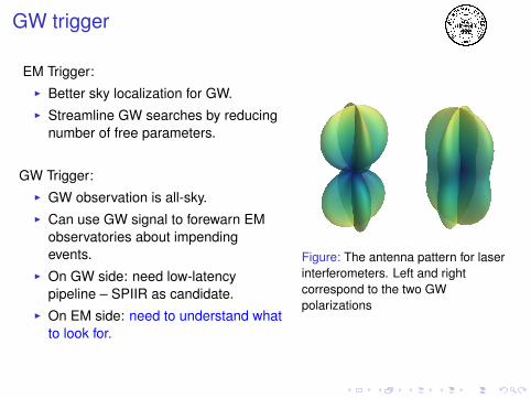
GW trigger
EM Trigger:I Better sky localization for GW.I Streamline GW searches by reducing
number of free parameters.
GW Trigger:I GW observation is all-sky.I Can use GW signal to forewarn EM
observatories about impendingevents.
I On GW side: need low-latencypipeline – SPIIR as candidate.
I On EM side: need to understand whatto look for.
Figure: The antenna pattern for laserinterferometers. Left and rightcorrespond to the two GWpolarizations
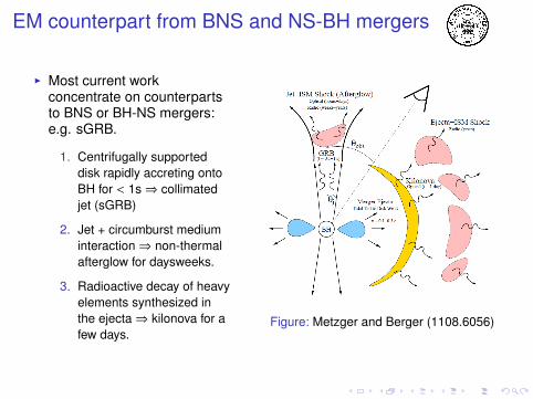
EM counterpart from BNS and NS-BH mergers
I Most current workconcentrate on counterpartsto BNS or BH-NS mergers:e.g. sGRB.
1. Centrifugally supporteddisk rapidly accreting ontoBH for < 1s⇒ collimatedjet (sGRB)
2. Jet + circumburst mediuminteraction⇒ non-thermalafterglow for daysweeks.
3. Radioactive decay of heavyelements synthesized inthe ejecta⇒ kilonova for afew days.
Figure: Metzger and Berger (1108.6056)
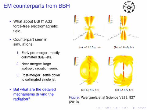
EM counterparts from BBH
I What about BBH? Addforce-free electromagneticfield.
I Counterpart seen insimulations.
1. Early pre-merger: mostlycollimated dual-jets.
2. Near-merger: largeisotropic radiation seen.
3. Post-merger: settle downto collimated single jet.
I But what are the detailedmechanisms driving theradiation? Figure: Palenzuela et al Science V329, 927
(2010).
Intro to FFE
I Idealized approximation to magnetosphere of neutron stars andblack holes, containing (B dominated) EM field and tenuous plasma.
I The B field:Inherited for neutron star.Accretion disk or ion-supported torus for black hole.
I The Plasma: ∼ strong B field⇒ E field when compact object present⇒ accelerate stray charged particles⇒ emit photon above mass of e− and e+ pair⇒ pair production and sequence repeats (cascade )⇒ e− and e+ short out E along B⇒ ∃ gaps to replenish lost plasma (”dynamical equilibrium”).
Intro to FFE
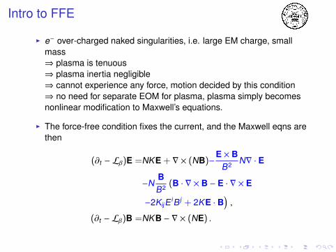
I e− over-charged naked singularities, i.e. large EM charge, smallmass⇒ plasma is tenuous⇒ plasma inertia negligible⇒ cannot experience any force, motion decided by this condition⇒ no need for separate EOM for plasma, plasma simply becomesnonlinear modification to Maxwell’s equations.
I The force-free condition fixes the current, and the Maxwell eqns arethen
(∂t − Lβ)E =NKE + ∇ × (NB)−E × B
B2 N∇ · E
−NBB2 (B · ∇ × B − E · ∇ × E
−2KijE iB j + 2KE · B),
(∂t − Lβ)B =NKB − ∇ × (NE) .
Spacetime approach to FFE
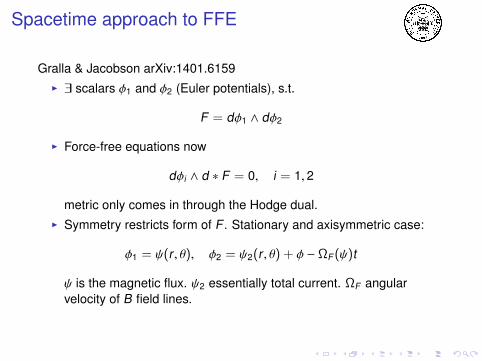
Gralla & Jacobson arXiv:1401.6159I ∃ scalars φ1 and φ2 (Euler potentials), s.t.
F = dφ1 ∧ dφ2
I Force-free equations now
dφi ∧ d ∗ F = 0, i = 1, 2
metric only comes in through the Hodge dual.I Symmetry restricts form of F . Stationary and axisymmetric case:
φ1 = ψ(r , θ), φ2 = ψ2(r , θ) + φ − ΩF (ψ)t
ψ is the magnetic flux. ψ2 essentially total current. ΩF angularvelocity of B field lines.
BBH stages
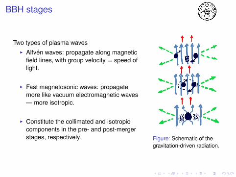
Two types of plasma wavesI Alfven waves: propagate along magnetic
field lines, with group velocity = speed oflight.
I Fast magnetosonic waves: propagatemore like vacuum electromagnetic waves— more isotropic.
I Constitute the collimated and isotropiccomponents in the pre- and post-mergerstages, respectively. Figure: Schematic of the
gravitation-driven radiation.
BBH pre-merger
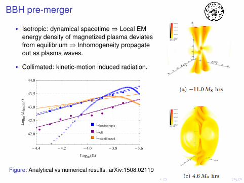
I Isotropic: dynamical spacetime⇒ Local EMenergy density of magnetized plasma deviatesfrom equilibrium⇒ Inhomogeneity propagateout as plasma waves.
I Collimated: kinetic-motion induced radiation.
æ
æ
æ
æ
æ
æ
æ
æ
æ
æ
ææ
ææ
æ
æ
æ
++
+
++
+
++++
+++++
+
+++++
+++++
++
+
+++++++
+++++++++
++++++++++++
+++++++++
++
++++++++++++++++++++++++++
+++++++++++++
++++++++++++++++++++++++++++++++++++++++++++++++++++++++++++++++++++++++++++++++++++++++++++++++
Lfastisotropic
LAlf
Lmcollimated
-4.4 -4.2 -4.0 -3.8 -3.6
42.0
42.5
43.0
43.5
44.0
Log10 HWL
Log 1
0HL f
astA
lfL
Figure: Analytical vs numerical results. arXiv:1508.02119
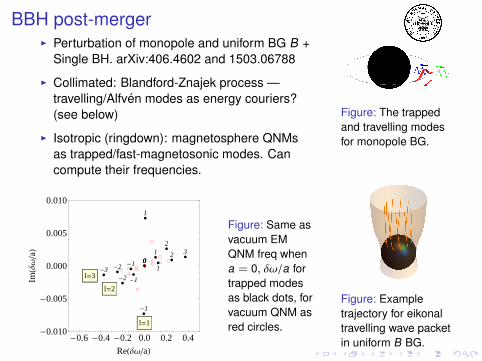
BBH post-mergerI Perturbation of monopole and uniform BG B +
Single BH. arXiv:406.4602 and 1503.06788
I Collimated: Blandford-Znajek process —travelling/Alfven modes as energy couriers?(see below)
I Isotropic (ringdown): magnetosphere QNMsas trapped/fast-magnetosonic modes. Cancompute their frequencies.
-1
0
1
-2 -1
01
232
10
-1-2
-3
- 1
0
1
- 2
- 1
0
1
2
3
2
1
0
- 1
- 2
- 3
-0.6 -0.4 -0.2 0.0 0.2 0.4-0.010
-0.005
0.000
0.005
0.010
ReH∆ΩaL
ImH∆
Ωa
L
l=1
l=2
l=3
Figure: Same asvacuum EMQNM freq whena = 0, δω/a fortrapped modesas black dots, forvacuum QNM asred circles.
Figure: The trappedand travelling modesfor monopole BG.
Figure: Exampletrajectory for eikonaltravelling wave packetin uniform B BG.
Future: better understanding of jets
I Final single jet: BZ solution is only for slow spin monopole orpoloidal BG, what of high spin? uniform BG?
I Early dual jets: analytical description of kinetic-motion jets?
I Efforts run into non-uniqueness: allowance for current enlarge spaceof possible solutions:
I Given an ΩF choice, often has a current that makes it happen (relatedby horizon BC), even with fixed BC at infinity (nonlinear eqns, nouniqueness?).
I Choose ΩF to satisfy additional symmetry etc to narrow down search.E.g. self-similar solution in NHEK (PRD 90, 124009, much more inLupsasca, Rodriguez, Strominger, arXiv:1406.4133, arXiv:1412.4124).
I Or get family of solutions “indexed” by ΩF . E.g. jet solutions of Gralla &Jacobson arXiv:1503.03848 (translationally symmetric) andarXiv:1503.06788 (axisymmetrically symmetric).
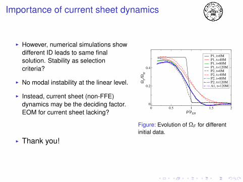
Importance of current sheet dynamics
I However, numerical simulations showdifferent ID leads to same finalsolution. Stability as selectioncriteria?
I No modal instability at the linear level.
I Instead, current sheet (non-FFE)dynamics may be the deciding factor.EOM for current sheet lacking?
I Thank you!
0 0.5 1 1.5 2ρ/ρEH
0
0.2
0.4
ΩF/ΩH
P1, t=0M
P1, t=40M
P1, t=80M
P1, t=120M
P2, t=0M
P2, t=40M
P2, t=80M
P2, t=120M
A1, t=120M
Figure: Evolution of ΩF for differentinitial data.
![Electromagnetic counterparts of gravitational wave transientsnuclphys.sinp.msu.ru/conf/epp10/Branchesi.pdf · fainter signals 1 t(year) 10 F v mJy F v [mJy] 100 10-1 100 10-1 10-2](https://img.pdfslide.us/doc/110x75/5c01b41509d3f20f068d2b9c/electromagnetic-counterparts-of-gravitational-wave-fainter-signals-1-tyear.jpg)