The Eﬁect of Supply Disruptions on Supply Chain …...Arreola-Risa (1994). His approximate cost function not only is convex but also yields a closed His approximate cost function

The Effect of Supply Disruptions on Supply Chain

Design Decisions

Lian Qi

Department of Business & Information Technology

Missouri University of Science & Technology, Rolla, MO

Zuo-Jun Max Shen

Department of Industrial Engineering & Operations Research

University of California, Berkeley, CA

Lawrence V. Snyder

Department of Industrial & Systems Engineering

Lehigh University, Bethlehem, PA

March 14, 2008

Abstract

We study an integrated supply chain design problem that determines the locations of retailers

and the assignments of customers to retailers in order to minimize the expected costs of location,

transportation, and inventory. The system is subject to random supply disruptions that may

occur at either the supplier or the retailers. Analytical and numerical studies reveal the effects

of these disruptions on retailer locations and customer allocations. In addition, we demonstrate

numerically that the cost savings from considering supply disruptions at the supply chain design

phase (rather than at the tactical or operational phase) are usually significant.

1

2

1 Introduction

Integrated supply chain design problems make facility location and demand assignment decisions

based on the locations and demand characteristics of fixed customers in order to minimize the

total cost (or maximize the total profit), including location, inventory and transportation costs.

It has been recently studied by many researchers, including Shen, Coullard and Daskin (2003),

Daskin, Coullard, and Shen (2002), Shu, Teo, and Shen (2005), and Shen and Qi (2007). Shen

(2007) provides a comprehensive literature review on integrated supply chain design problems.

The existing research on integrated supply chain design problems assumes that the suppliers and

facilities in supply chain networks are always available to serve their customers. However, supply

chain disruptions are possible at any stage of a supply chain network, and failing to plan for them

adequately may result in significant economic losses.

Recent examples of supplier/facility disruptions include:

• The west-coast port lockout in 2002 and the subsequent inventory shortages caused factories

across a variety of industries to close and perishable cargo to rot. Economists estimated

damage to the economy at $1 billion a day (Greenhouse, 2002).

• The logistical logjam due to the disruptions of numerous facilities after hurricanes Katrina and

Rita caused a huge economic loss in 2005 (Barrionuevo and Deutsch, 2005). For example,

124 local Wal-Mart stores and two distribution centers were shut down, and fifteen stores

remained closed half a month after Hurricane Katrina (Halkias, 2005).

We learn from these examples that supplier and facility disruptions should be both considered

in integrated supply chain design problems so that the facilities’ locations are determined with the

possible losses caused by facility disruptions taken into consideration and the inventory decisions

at the facilities are made to protect against supplier disruptions.

3

In summary, we believe that it is important for supply chain designers and managers to be able

to address the following questions:

• What are the impacts of disruptions both at internal facilities and at those facilities’ suppliers

on the optimal facility location and demand-allocation decisions?

• Can significant cost savings be achieved in practice if we consider supply disruptions at the

supply chain design phase?

We explore answers to these questions, borrowing ideas from inventory management problems

with supply disruptions, such as the models of Parlar and Berkin (1991), Berk and Arreola-Risa

(1994), Snyder (2005), Qi, Shen and Snyder (2007), and Tomlin (2006).

Specifically, we consider the following single-product problem: Customers are distributed through-

out a certain region. We wish to open one or more retailers that are served directly from a supplier

whose location is fixed. The retailers satisfy deterministic demands from the customers and place

replenishment orders to the supplier. We assume zero lead time for order processing at the supplier

and retailers when non-disrupted. However, both the supplier and the retailers may be disrupted

randomly:

• When a retailer is disrupted, it becomes unavailable, and no customer demand received during

the disruption can be filled until the disruption has ended. In addition, any inventory on hand

at the retailer is destroyed when the disruption occurs.

• If a retailer wishes to place an order when the supplier is disrupted, this order will not be

filled until the supplier recovers from the disruption. Hence, a retailer may not be able to

serve its customers even if it is available itself, since it may have no inventory on hand due

to the delayed shipment from the disrupted supplier.

If a customer is assigned to a retailer but the retailer is disrupted or out of stock, the unmet

demands are backlogged, at a cost. We assume that customers may not be temporarily reassigned

4

to non-disrupted retailers if their own assigned retailer is disrupted or out of stock; that is, we

do not consider dynamic sourcing. In addition, we allow some customers not to be served at all,

even when no disruptions have occurred, if the cost of serving them is prohibitive. In this case, a

lost-sales penalty is applied for each unit of unserved customer demand.

We formulate an integrated model to determine 1) how many retailers should be opened, and

where to locate them; 2) which retailers should serve which customers; and 3) how often and how

much to order at each retailer, so as to minimize the total location, working inventory (including or-

dering, holding and backorder costs), transportation, and lost-sales costs. Since customer demands

are deterministic, the inventory at each retailer serves two main purposes: 1) to take advantage of

economies of scale due to fixed costs, and 2) to protect against supplier disruptions.

We analyze this model to evaluate the impact of random supply disruptions at the supplier

and retailers on the retailer location and customer demand allocation decisions. We use numerical

experiments to verify the conclusions made in our analytical studies. Our results show that sig-

nificant cost savings can often be achieved if we consider supply disruptions when making supply

chain design decisions.

The remainder of this paper is organized as follows. In Section 2, we review the related literature.

We then propose an integrated supply chain design model in Section 3 for the problem stated above.

We analyze the model in Section 4 to evaluate the impact of supply disruptions on facility location

and demand assignment decisions. We suggest a solution algorithm in Section 5 for the model, and

conduct numerical experiments in Section 6 to further study the impact of supply disruptions and

explore the conditions under which significant cost savings can be achieved by considering supply

disruptions during the supply chain design phase. We conclude our work in Section 7, and suggest

some future research directions.

5

2 Literature Review

The study by Parlar and Berkin (1991) is among the earliest works that incorporate supply disrup-

tions into classical inventory models. They consider a variant of the EOQ model in which supply is

available during an interval of random length and then unavailable for another interval of random

length. Their model assumes that the firm knows the availability status of the supplier and that

it follows a zero-inventory ordering (ZIO) policy. Berk and Arreola-Risa (1994) show that Parlar

and Berkin’s original model is incorrect in two respects. Their corrected cost function cannot be

minimized in closed form, nor is it known whether it is convex.

Snyder (2005) develops an effective approximation for the model introduced by Berk and

Arreola-Risa (1994). His approximate cost function not only is convex but also yields a closed-

form solution and behaves similarly to the classical EOQ cost function in several important ways.

Heimann and Waage (2005) relax the ZIO assumption in Snyder’s model and derive a closed-form

approximate solution.

Parlar and Perry (1995) relax the two assumptions made in (1991). First, they consider the

case in which the decision maker is not aware of the ON-OFF status of the supply before an order

is placed. Second, their model allows the reorder point to be a decision variable. In addition

to random supply disruptions, Gupta (1996) assumes that the customer demands are random,

generated according to a Poisson process. He considers constant lead times, whereas Parlar (1997)

introduces a more general model in which the lead time may be stochastic.

Qi, Shen and Snyder (2007) extend the works of Berk and Arreola-Risa (1994) and Snyder (2005)

by considering random disruptions at two echelons—at the supplier (as in Berk and Arreola-Risa,

1994, and Snyder, 2005) and at the retailers. They conduct analytical and numerical studies to

determine the impact of supply disruptions on the retailer’s optimal inventory decisions. They also

propose an effective approximation of their cost function that we embed into the objective function

of our integrated model in the present paper. Qi, Shen and Snyder prove that their approximation

6

is a concave and increasing function of the total demand the retailer faces, a property that we make

use of in the present paper.

The above works assume there is only one supplier, and if that supplier is disrupted, the firm

has no recourse. In contrast, Tomlin (2006) presents a dual-sourcing model in which orders may

be placed with either a cheap but unreliable supplier or an expensive but reliable supplier. He

considers a very general stochastic recovery process at the unreliable supplier. He evaluates the

firm’s optimal strategy under various realizations of the problem parameters.

Since this paper considers multiple retailers in an integrated supply chain design setting, our

work is also closely related to the literature on integrated supply chain design. Shen, Coullard

and Daskin (2003), Daskin, Coullard, and Shen (2002) study a joint location/inventory model in

which location, shipment and nonlinear inventory costs are included in the same model. They

develop an integrated approach to determine the number of distribution centers (DCs) to establish,

the location of the DCs, the assignments of customers to DCs, and the magnitude of inventory

to maintain at each DC. More general problems are studied by Shu, Teo, and Shen (2005), Shen

and Qi (2007), and Snyder, Daskin, and Teo (2007). None of these integrated supply chain design

problems consider random supply disruptions.

Our paper is also closely related to the literature on facility location with disruptions. Snyder

and Daskin (2005) consider facility location models in which some facilities will fail with a given

probability. Their models are based on two classical facility location models and assume that

customers may be re-assigned to alternate DCs if their closest DC is disrupted. Their models

minimize a weighted sum of the nominal cost (which is incurred when no disruptions occur) and

the expected transportation cost accounting for disruptions. They do not consider inventory costs.

Related models are studied by Berman, Krass, and Menezes (2007), Church and Scaparra (2007),

and Scaparra and Church (2008). Snyder and Daskin (2007) compare models for reliable facility

location under a variety of risk measures and operating strategies. Snyder, Scaparra, Daskin,

7

and Church (2006) provide a tutorial and literature review for supply chain design models with

disruptions.

Like our paper, Berman, Krass, and Menezes (2007), Church and Scaparra (2007), Scaparra

and Church (2008), Snyder and Daskin (2005), Snyder and Daskin (2007), Snyder et al. (2006)

consider facility location with disruptions. Our paper differs from the earlier literature in two main

respects. First, we consider the cost of inventory at the facilities, optimizing the inventory levels to

account for supplier disruptions. Second, we consider disruptions at both the supplier and at the

retailers, whereas the earlier literature considers disruptions only at the retailers.

Finally, we mention two additional papers on supply chain design under supply uncertainty:

those of Qi and Shen (2007) and Kim, Lu and Kvam (2005). Both papers consider yield uncer-

tainty/product defects in supply chain design decisions for a three-echelon supply chain using ideas

from the random yield literature. However, supply disruptions are not considered in these papers.

3 Model Formulation

3.1 Notation and Formulation

In this section, we formulate an integrated model for the problem stated in Section 1. The objective

is to minimize the expected total annual cost including 1) the fixed cost to open retailers, 2) the

working inventory cost (including ordering, holding and backorder costs) at the open retailers; 3)

the transportation cost from retailers to customers; and 4) the lost-sales penalty cost of choosing

not to serve some customers. (Although we use one year as the time horizon for our model, it can

easily be adapted for other time units.)

We use the following notation throughout the paper:

I: index set of all customers

J : index set of candidates locations for retailers

8

Di: annual demand of customer i ∈ I

fj : annual fixed cost to open a retailer at location j ∈ J

π: penalty cost for not assigning a customer to any retailer, per unit of demand

Tj(·): the working inventory cost at retailer j ∈ J (This includes ordering, holding, and backo-

rder costs at retailer j and is a function of the total demand assigned to j. It is zero if no retailer

is opened at location j. We examine Tj(·) in greater detail in Section 3.2.)

dij : unit cost to deliver items from retailer j ∈ J to customer i ∈ I

There are two sets of decision variables:

Xj= 1 if a retailer is opened at site j ∈ J , 0 otherwise;

Yij= 1 if the demand from customer i ∈ I is to be served by the retailer at site j ∈ J , 0 otherwise.

It is expedient to create a “dummy” retailer with index s; assigning a customer i to this retailer

(Yis = 1) represents not assigning the customer at all. We therefore formulate our problem as

minimize∑

j∈J

{fjXj + Tj

(∑

i∈I

DiYij

)+

∑

i∈I

dijDiYij

}+ π

∑

i∈I

DiYis (1)

subject to∑

j∈J

Yij + Yis = 1 ∀i ∈ I (2)

Yij −Xj ≤ 0 ∀i ∈ I, j ∈ J (3)

Yij ∈ {0, 1} ∀i ∈ I, j ∈ J ∪ {s} (4)

Xj ∈ {0, 1} ∀j ∈ J (5)

The first three terms in the objective function represent the annual fixed cost to open retail-

9

ers, the working inventory cost at open retailers, and the retailer–customer transportation cost,

respectively. (The transportation cost from the supplier to the retailers is included in Tj(·), as

discussed in Section 3.2.) The last term in the objective function represents the lost-sales cost for

those customers not served by any retailer. The constraints of the above model are similar to those

of other well known warehouse location problems, such as the one studied by Erlenkotter (1978).

In particular, (2) requires each customer to be assigned to exactly one retailer or to the “dummy”

retailer. Constraint (3) requires customers to be served only by open retailers. Constraints (4) and

(5) are standard integrality constraints.

This is a single-sourcing model since each customer may be served by only one retailer (either

a real retailer or the dummy retailer). One could consider a multiple-sourcing option, in which a

customer may be served by more than one retailer, simply by replacing (4) with Yij ∈ [0, 1]. The

resulting model has a convex (linear) feasible region and therefore will attain its minimum at an

extreme point if the objective function is concave. In other words, the multiple-sourcing constraint

Yij ∈ [0, 1] reduces to (4) if the objective function is concave. As we will prove in Section 3.2, the

form we will use for Tj(·) is concave in the demand assigned to retailer j. Therefore, we consider

only the single-sourcing version of the model in the remainder of this paper.

We define Dj(Y ) =∑

i∈I DiYij to simplify the notation. Replacing Yis in (1) with 1−∑i∈I Yij

according to (2) and omitting the constant term π∑

i∈I Di, the original problem may be rewritten

as follows:

(P) : minimize∑

j∈J

{fjXj + Tj(Dj(Y )) +

∑

i∈I

(dij − π)DiYij

}

subject to∑

j∈J

Yij ≤ 1 ∀i ∈ I

Yij −Xj ≤ 0 ∀i ∈ I, j ∈ J

Yij ∈ {0, 1} ∀i ∈ I, j ∈ J

10

Xj ∈ {0, 1} ∀j ∈ J

3.2 Formulation and Approximation of Tj(·)

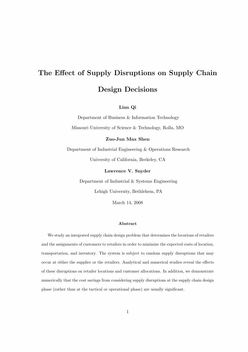
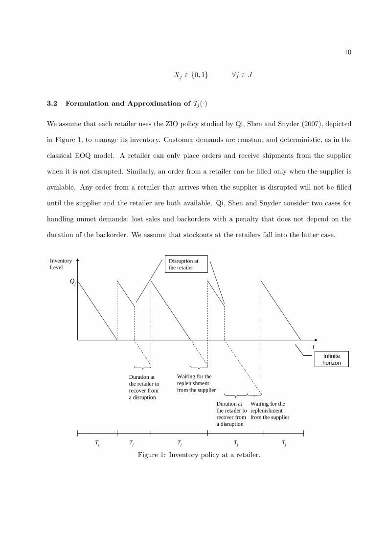
We assume that each retailer uses the ZIO policy studied by Qi, Shen and Snyder (2007), depicted

in Figure 1, to manage its inventory. Customer demands are constant and deterministic, as in the

classical EOQ model. A retailer can only place orders and receive shipments from the supplier

when it is not disrupted. Similarly, an order from a retailer can be filled only when the supplier is

available. Any order from a retailer that arrives when the supplier is disrupted will not be filled

until the supplier and the retailer are both available. Qi, Shen and Snyder consider two cases for

handling unmet demands: lost sales and backorders with a penalty that does not depend on the

duration of the backorder. We assume that stockouts at the retailers fall into the latter case.

t

Qj

Disruption at the retailer

Waiting for the replenishment from the supplier

Tj

Infinite horizon

Inventory Level

Duration at the retailer to recover from a disruption

Duration at the retailer to recover from a disruption

Waiting for the replenishment from the supplier

Tj Tj Tj Tj

Figure 1: Inventory policy at a retailer.

11

We define

Fj : fixed ordering cost at retailer j ∈ J

aj : per-unit ordering cost at retailer j ∈ J

hj : annual holding cost per item at retailer j ∈ J

πj : time-independent backorder cost per unit of unmet demand at retailer j ∈ J (typically,

aj < πj)

Tj : the inventory cycle length at retailer j ∈ J , equal to the duration between two consecutive

shipments from the supplier to retailer j (a random variable)

Qj : the inventory level at retailer j ∈ J at the beginning of each inventory cycle; the order size

from retailer j to the supplier is therefore Qj plus any backlogged demand (Qj is a decision variable;

however, we will express the optimal inventory cost in closed form without using Qj explicitly in

the objective function)

The retailers and supplier both experience ON (available) and OFF (disrupted) cycles of ran-

dom durations. We assume that the durations of the ON and OFF cycles at the supplier follow

independently and identically distributed (iid) exponential distributions with rates λ and ψ, respec-

tively; and that the durations of the ON and OFF cycles at retailer j ∈ J follow iid exponential

distributions with rates αj and βj , respectively. To summarize:

λ: disruption rate at the supplier (times/year)

ψ: recovery rate at the supplier (times/year)

αj : disruption rate at retailer j ∈ J (times/year)

βj : recovery rate at retailer j ∈ J (times/year)

Following Qi, Shen, and Snyder (2007), we further assume that all inventory at a retailer is

destroyed if the retailer is disrupted.

12

If Dj(Y ) > 0, Qi, Shen, and Snyder (2007) proves that the expected annual working inventory

cost (including ordering, holding, and backorder costs) at retailer j is given by:

Ij(Qj) ≡ πjDj(Y ) +Fj +

(aj + hj

αj

)Qj −

(1− e

−αjQj

Dj(Y )

) [hjDj(Y )

α2j

+ πjDj(Y )αj

]

E[Tj ](6)

where

E[Tj ] = Aj

[1− e

−(αj+λ+ψ)Qj

Dj(Y )

]+ Bj

[1− e

− αjQjDj(Y )

]

Aj =λ

βjψ· αj + βj

αj + λ + ψ

Bj =1αj

+1βj

Let Q∗j = argminQ{Ij(Qj)}. Then Tj(Dj(Y )), the optimal working inventory cost at retailer

j ∈ J in (1), is equal to Ij(Q∗j ) when Dj(Y ) > 0 and to 0 otherwise.

Qi, Shen and Snyder (2007) suggest efficient solution algorithms to compute Q∗j based on the

cost function (6). Unfortunately, it is difficult to analyze (P) or to solve it using standard algorithms

since Tj(Dj(Y )) cannot be written in closed form without solving a separate non-linear optimization

problem. Though numerical experiments by Qi, Shen, and Snyder (2007) suggest that Tj(Dj(Y ))

is concave when considered as a function of Dj(Y ), they do not prove this rigorously, nor does the

exact cost function permit a closed-form expression for the optimal cost.

Instead, we use the following approximation for Tj(Dj(Y )):

Tj(Dj(Y )) =

πjDj(Y ) +Fj+

(aj−πj)Dj(Y )

αj+

(aj+

hjαj

)Qj

Aj+Bj, Dj(Y ) > 0

0 , Dj(Y ) = 0(7)

13

and the following approximation for Q∗j :

Qj = Dj(Y ) ·−Aj +

√

A2j +

2αj(Aj+Bj)

[αjFjBjDj(Y )

+Aj(πj−aj)

]

(αjaj+hj)

(Aj + Bj)αj, (8)

both of which are proposed by Qi, Shen, and Snyder (2007).

Tj(Dj(Y )) has an important property, stated in the following theorem.

Theorem 1 (Qi, Shen and Snyder, 2007) Tj(Dj(Y )) is a concave and increasing function of

Dj(Y ), the total demand that retailer j serves.

We replace Tj(·) in the objective function of (P) using its approximation Tj(·). The objective

function of (P) is thus approximated by:

∑

j∈J


∑

i∈I

(dij − π)DiYij

}(9)

We use (P) to denote the problem that minimizes (9) subject to the same constraints as (P). In

the following sections, we analytically and numerically study (P).

4 Model Analysis

It follows from (8) that

Qj =−Aj

(Aj + Bj)αj·Dj(Y )

+

√√√√[

A2j

(Aj + Bj)2α2j

+2Aj(πj − aj)

(αjaj + hj)(Aj + Bj)αj

]D2

j (Y ) +2FjBjDj(Y )

(αjaj + hj)(Aj + Bj)

= −Cj ·Dj(Y ) +

√(C2

j + 2CjKj

)D2

j (Y ) +2Fj(1− αjCj)Dj(Y )

αjaj + hj,

14

where we define

Cj =Aj

(Aj + Bj)αj=

λ

(ψ + αj)(ψ + λ)

Kj =πj − aj

αjaj + hj

to simplify the notation.

Furthermore, we have

∂

∂Dj(Y )Qj = −Cj +

(C2

j + 2CjKj

)Dj(Y ) + Fj(1−αjCj)

αjaj+hj√(C2

j + 2CjKj

)D2

j (Y ) + 2Fj(1−αjCj)Dj(Y )αjaj+hj

(10)

∂2

∂D2j (Y )

Qj = −[

Fj(1−αjCj)αjaj+hj

]2

[√(C2

j + 2CjKj

)D2

j (Y ) + 2Fj(1−αjCj)Dj(Y )αjaj+hj

]3

= −[

Fj

αjaj+hj

]2 √1− αjCj

[√Cj

1−αjCj· (Cj + 2Kj

)D2

j (Y ) + 2FjDj(Y )αjaj+hj

]3 < 0 (11)

Let

Lj = πj − αjaj + hj

αj(Aj + Bj)· (Cj + Kj −

√C2

j + 2Cj ·Kj). (12)

Lemma 1 Lj provides a lower bound on the marginal working inventory cost at retailer j ∈ J

regardless of the demand already assigned to this retailer.

Proof It follows from (10) and (11) that

∂

∂Dj(Y )Qj > −Cj +

√C2

j + 2CjKj for Dj(Y ) ≥ 0.

Therefore, the following inequality can be derived from (7):

∂

∂Dj(Y )Tj(Dj(Y )) > πj +

aj−πj

αj+ (aj + hj

αj)(−Cj +

√C2

j + 2Cj ·Kj)

Aj + Bj

15

= πj − αjaj + hj

αj(Aj + Bj)· (Cj + Kj −

√C2

j + 2Cj ·Kj)

= Lj ,

as desired.

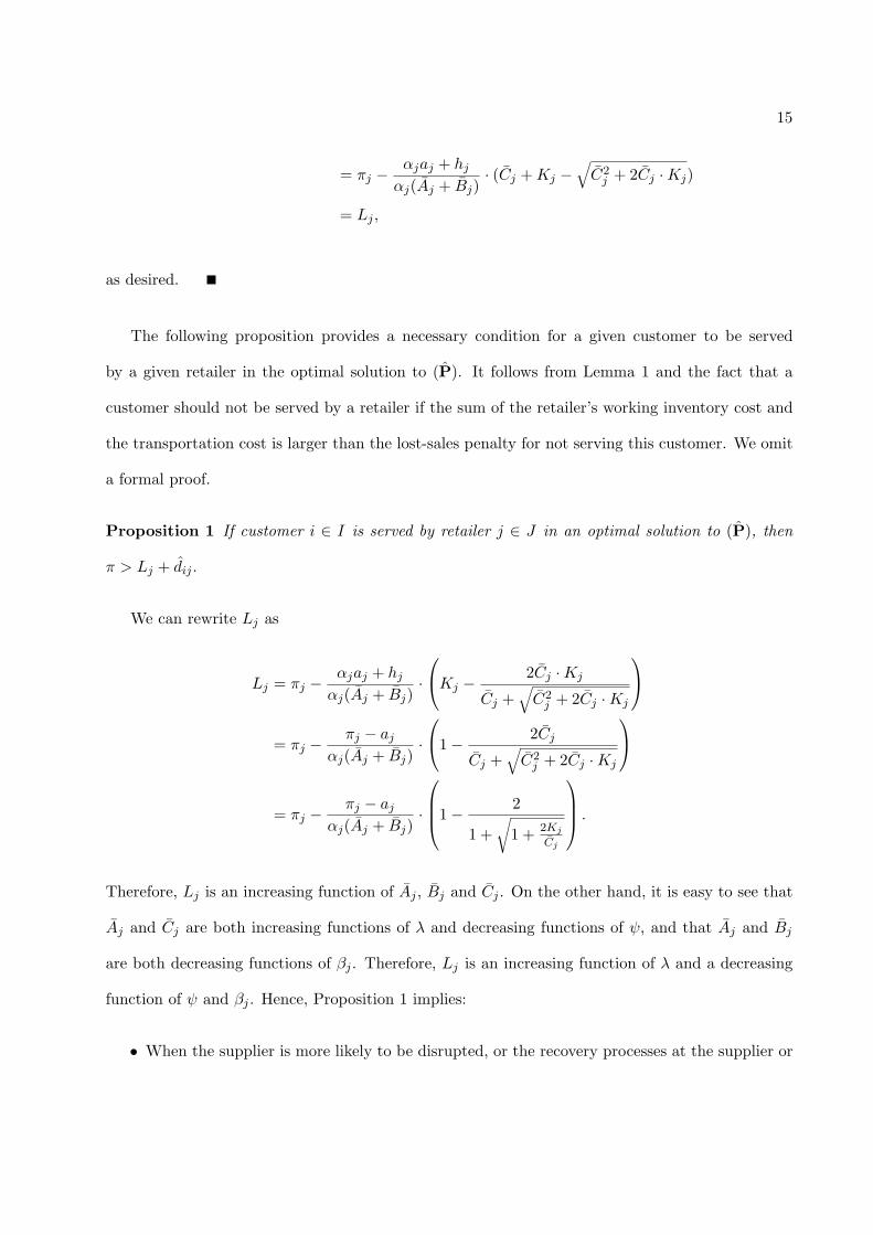
The following proposition provides a necessary condition for a given customer to be served

by a given retailer in the optimal solution to (P). It follows from Lemma 1 and the fact that a

customer should not be served by a retailer if the sum of the retailer’s working inventory cost and

the transportation cost is larger than the lost-sales penalty for not serving this customer. We omit

a formal proof.

Proposition 1 If customer i ∈ I is served by retailer j ∈ J in an optimal solution to (P), then

π > Lj + dij .

We can rewrite Lj as

Lj = πj − αjaj + hj

αj(Aj + Bj)·Kj − 2Cj ·Kj

Cj +√

C2j + 2Cj ·Kj

= πj − πj − aj

αj(Aj + Bj)·1− 2Cj

Cj +√

C2j + 2Cj ·Kj

= πj − πj − aj

αj(Aj + Bj)·

1− 2

1 +√

1 + 2Kj

Cj

.

Therefore, Lj is an increasing function of Aj , Bj and Cj . On the other hand, it is easy to see that

Aj and Cj are both increasing functions of λ and decreasing functions of ψ, and that Aj and Bj

are both decreasing functions of βj . Therefore, Lj is an increasing function of λ and a decreasing

function of ψ and βj . Hence, Proposition 1 implies:

• When the supplier is more likely to be disrupted, or the recovery processes at the supplier or

16

retailers are slower, fewer customers should be served by each open retailer, and the optimal

solution will involve more customers not served by any retailer.

• Retailers are more likely to be opened at locations with quick recoveries, and customers are

more likely to be served by retailers at these locations.

These conclusions conform with our intuition that to improve the service level or reduce the

extra operational costs caused by disruptions, reliable suppliers are preferred, and retailers should

be opened in low risk areas.

We are not able to analyze the impact of αj on the supply chain design decisions because of

the complexity of Lj as a function of αj . We numerically study these effects in Section 6.2.

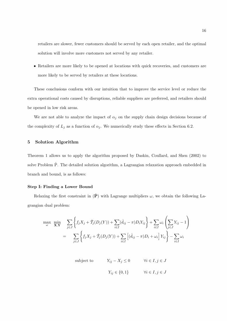
5 Solution Algorithm

Theorem 1 allows us to apply the algorithm proposed by Daskin, Coullard, and Shen (2002) to

solve Problem P. The detailed solution algorithm, a Lagrangian relaxation approach embedded in

branch and bound, is as follows:

Step I: Finding a Lower Bound

Relaxing the first constraint in (P) with Lagrange multipliers ω, we obtain the following La-

grangian dual problem:

maxω

minX,Y

∑

j∈J


∑

i∈I

(dij − π)DiYij

}+

∑

i∈I

ωi

∑

j∈J

Yij − 1

=∑

j∈J


∑

i∈I

[(dij − π)Di + ωi

]Yij

}−

∑

i∈I

ωi

subject to Yij −Xj ≤ 0 ∀i ∈ I, j ∈ J

Yij ∈ {0, 1} ∀i ∈ I, j ∈ J

17

Xj ∈ {0, 1} ∀j ∈ J

ωi ≥ 0 ∀i ∈ I

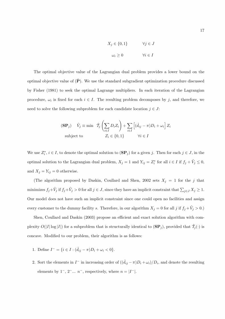
The optimal objective value of the Lagrangian dual problem provides a lower bound on the

optimal objective value of (P). We use the standard subgradient optimization procedure discussed

by Fisher (1981) to seek the optimal Lagrange multipliers. In each iteration of the Lagrangian

procedure, ωi is fixed for each i ∈ I. The resulting problem decomposes by j, and therefore, we

need to solve the following subproblem for each candidate location j ∈ J :

(SPj) Vj ≡ min Tj

(∑

i∈I

DiZi

)+

∑

i∈I

[(dij − π)Di + ωi

]Zi

subject to Zi ∈ {0, 1} ∀i ∈ I

We use Z∗i , i ∈ I, to denote the optimal solution to (SPj) for a given j. Then for each j ∈ J , in the

optimal solution to the Lagrangian dual problem, Xj = 1 and Yij = Z∗i for all i ∈ I if fj + Vj ≤ 0,

and Xj = Yij = 0 otherwise.

(The algorithm proposed by Daskin, Coullard and Shen, 2002 sets Xj = 1 for the j that

minimizes fj+Vj if fj+Vj > 0 for all j ∈ J , since they have an implicit constraint that∑

j∈J Xj ≥ 1.

Our model does not have such an implicit constraint since one could open no facilities and assign

every customer to the dummy facility s. Therefore, in our algorithm Xj = 0 for all j if fj + Vj > 0.)

Shen, Coullard and Daskin (2003) propose an efficient and exact solution algorithm with com-

plexity O(|I| log |I|) for a subproblem that is structurally identical to (SPj), provided that Tj(·) is

concave. Modified to our problem, their algorithm is as follows:

1. Define I− = {i ∈ I : (dij − π)Di + ωi < 0}.

2. Sort the elements in I− in increasing order of ((dij −π)Di +ωi)/Di, and denote the resulting

elements by 1−, 2−... n−, respectively, where n = |I−|.

18

3. Find the value of m (1 ≤ m ≤ n) that minimizes

Tj

(m∑

i=1

Di−Zi−

)+

m∑

i=1

[(di−j − π)Di− + ωi−

]Zi− .

4. Then an optimal solution to subproblem (SPj) is given by Z1− = Z2− = ... = Zm− = 1 and

Zi = 0 for all other i ∈ I.

Step II: Finding an Upper Bound

In each iteration of the Lagrangian procedure, we derive a feasible solution to Problem P based

on the current Lagrangian solution by assigning each customer to one and only one retailer.

Note that assigning customers optimally to a fixed set of open retailers is not trivial in our

problem, as it is in most linear facility location problems. Although the customer-assignment

problem is polynomially solvable for a fixed number of open retailers (it is a special case of the

[PTP(k)] problem discussed by Tuy et al., 1996), exact algorithms for this problem, such as the one

proposed by Tuy et al., are impractical when the number of retailers is reasonably large. Therefore,

we employ the following heuristic procedure, adapted from Shen, Coullard and Daskin (2003), to

assign customers to retailers:

1. For each customer i ∈ I, let Ji be the set of potential retailer sites (Ji ⊆ J) that customer i

is assigned to in the Lagrangian solution. If Ji 6= ∅, we assign customer i to the retailer in

Ji ∪ {s} that results in the least increase in cost. If Ji = ∅, we assign this customer to the

dummy retailer s.

2. We close all open retailers that no longer serve any customers after performing step 1.

If the objective value of (P) under the resulting feasible solution is less than the current upper

bound, we take the objective value of the new solution as the new upper bound, and further improve

it using Step III. (One may choose to perform Step III even if the new solution is not better than

19

the best known solution. However, we found that this strategy does not significantly enhance the

algorithm’s performance and in many cases makes the algorithm slower.)

Step III: Customer Reassignment

1. For each i ∈ I, we search the other open retailers (including the dummy retailer s) to see

whether the cost would decrease if we assigned i instead to that retailer. We perform the

best improving swap found.

2. We close all open retailers that no longer serve any customers after performing step 1.

We then recalculate the objective value of (P) with the new feasible solution obtained in this

step, and update the upper bound if necessary.

Step IV: Variable Fixing

At the end of each iteration of the Lagrangian procedure, we employ the following two rules

to see whether some of the Xj variables can be fixed. (See Shu, Teo, and Shen, 2005 for detailed

proofs of the validity of these rules.)

Let LB and UB be the current lower and upper bounds on the optimal objective value, respec-

tively.

Rule 1: If no retailer is opened at candidate location j ∈ J in the Lagrangian solution obtained

in Step I, and if LB + fj + Vj > UB, then no retailer will be opened at j in any optimal solution

to (P), so we fix Xj = 0.

Rule 2: If a retailer is opened at candidate location j ∈ J in the Lagrangian solution obtained

in Step I, and if LB− (fj + Vj) > UB, then a retailer will be opened at j in every optimal solution

to (P), so we fix Xj = 1.

If the lower and upper bounds are sufficiently close (please refer to Table 1), or if all candidate

locations are fixed with the above two rules, we terminate the Lagrangian procedure. In either of

20

these cases, the solution corresponding to the upper bound is a (near-)optimal solution to (P). We

also stop the Lagrangian procedure based on certain conditions regarding the current Lagrangian

settings (please refer to Table 1); in this case, we conduct branch and bound, branching on the

unfixed location variables (Xj , j ∈ J).

Proposition 1 can also be used to filter out solutions that are impossible to make the algorithm

more efficient. Based on this proposition, customer i ∈ I should not be served by retailer j ∈ J in

the optimal solution if π ≤ Lj + dij .

6 Numerical Experiments

In this section, we report the results of our computational experiments to verify the conclusions

drawn in Section 4. We also study the benefit of considering supply disruptions during the supply

chain design phase.

We conduct computational experiments on the 88-node and 150-node data sets described by

Daskin (1995). The weight factors associated with the transportation and inventory costs we used

in our experiments on the 88-node data set are 0.005 and 0.1, respectively, and those we used in

experiments on the 150-node data set are 0.0008 and 0.01, respectively. We fix the per-unit penalty

cost for not serving customers, π, which is not included in the original data sets, to be 25. As

in Daskin, Coullard and Shen (2002), we fix the fixed ordering cost, unit ordering cost and unit

holding cost at retailer j ∈ J (Fj , aj and hj) to be 10, 5, and 1, respectively.

Table 1 lists the parameters we used for the Lagrangian relaxation procedure in our computa-

tional experiments. Please refer to Fisher (1981) and Daskin, Coullard, and Shen (2002) for more

details on the interpretation of these parameters. With these parameters, the algorithm solved the

problems within 10 seconds for most instances associated with the 88-node data set and within 60

seconds for most instances associated with the 150-node data set. We do not provide a detailed

report of the computational performance of the algorithm, since its efficiency has already been

21

documented by Daskin, Coullard and Shen (2002), Shen and Qi (2007), Snyder, Daskin, and Teo

(2004) and others.

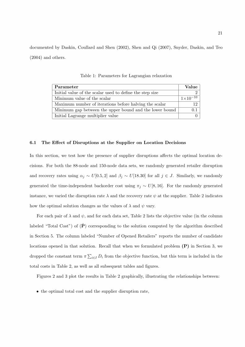
Table 1: Parameters for Lagrangian relaxation

Parameter ValueInitial value of the scalar used to define the step size 2Minimum value of the scalar 1×10−10

Maximum number of iterations before halving the scalar 12Minimum gap between the upper bound and the lower bound 0.1Initial Lagrange multiplier value 0

6.1 The Effect of Disruptions at the Supplier on Location Decisions

In this section, we test how the presence of supplier disruptions affects the optimal location de-

cisions. For both the 88-node and 150-node data sets, we randomly generated retailer disruption

and recovery rates using αj ∼ U [0.5, 2] and βj ∼ U [18.30] for all j ∈ J . Similarly, we randomly

generated the time-independent backorder cost using πj ∼ U [8, 16]. For the randomly generated

instance, we varied the disruption rate λ and the recovery rate ψ at the supplier. Table 2 indicates

how the optimal solution changes as the values of λ and ψ vary.

For each pair of λ and ψ, and for each data set, Table 2 lists the objective value (in the column

labeled “Total Cost”) of (P) corresponding to the solution computed by the algorithm described

in Section 5. The column labeled “Number of Opened Retailers” reports the number of candidate

locations opened in that solution. Recall that when we formulated problem (P) in Section 3, we

dropped the constant term π∑

i∈I Di from the objective function, but this term is included in the

total costs in Table 2, as well as all subsequent tables and figures.

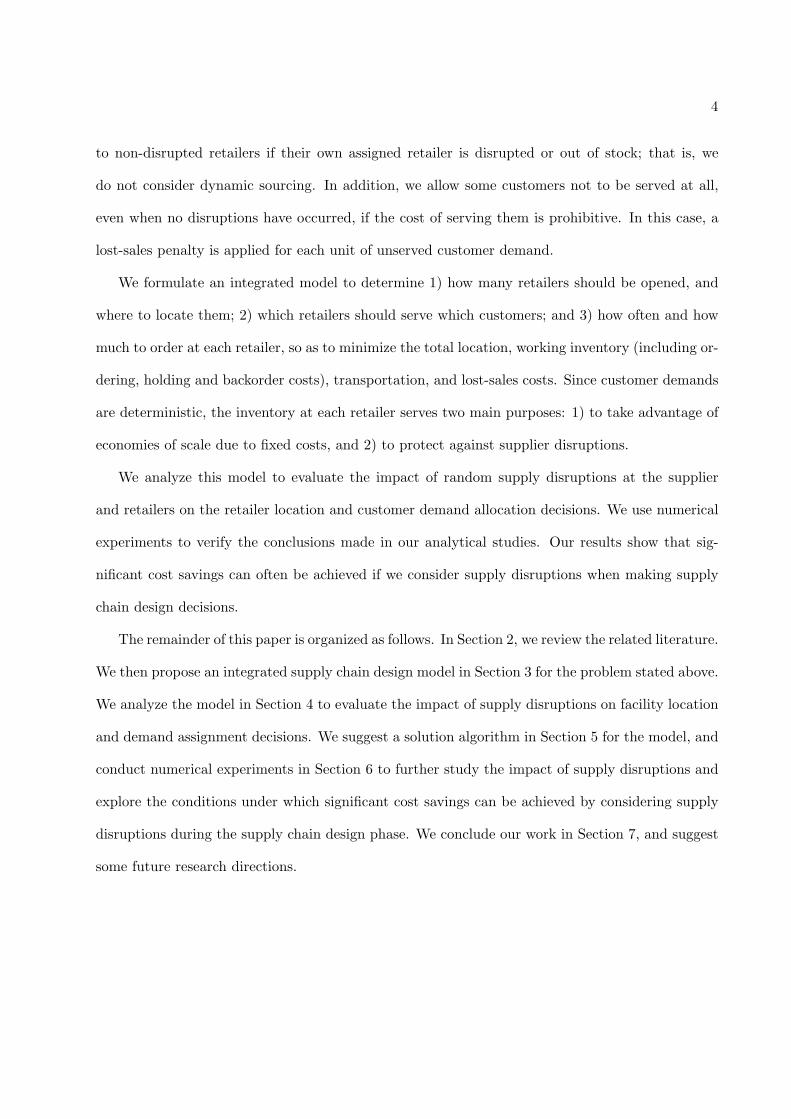
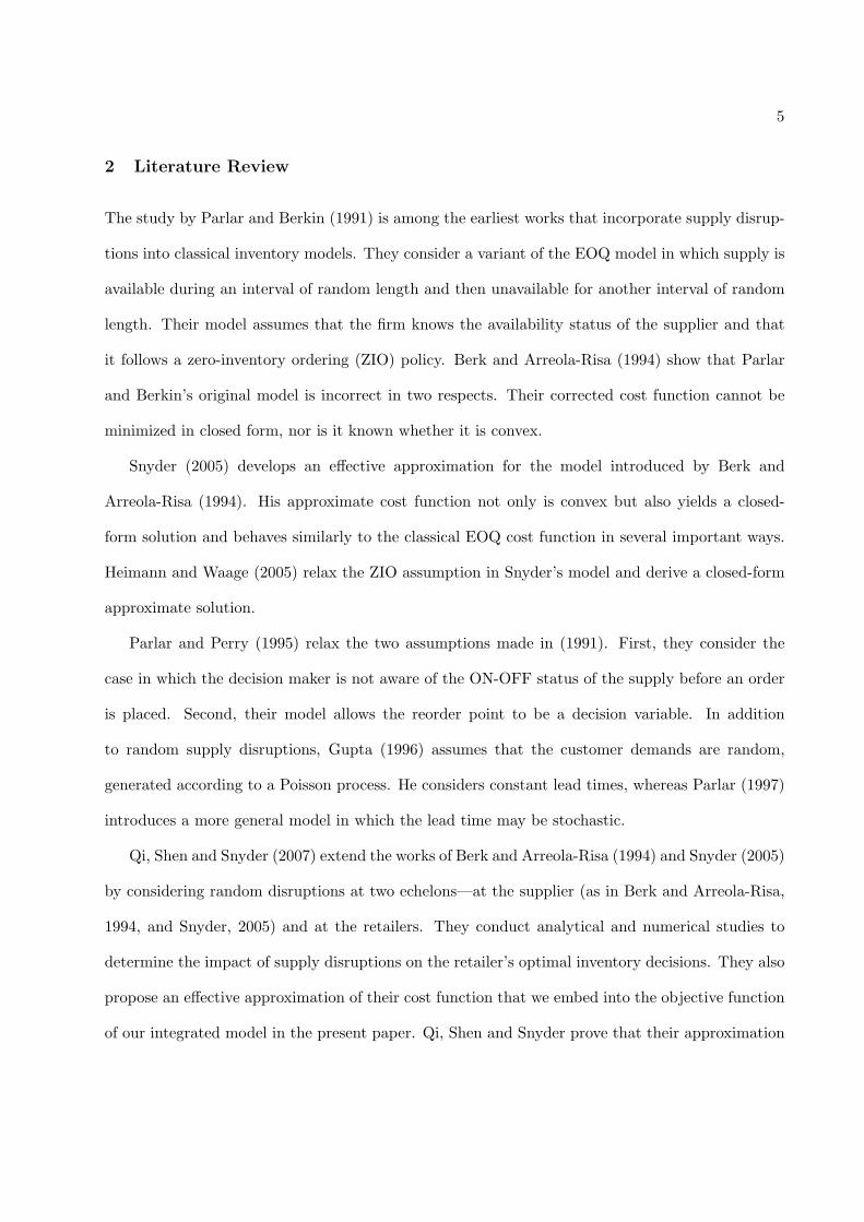
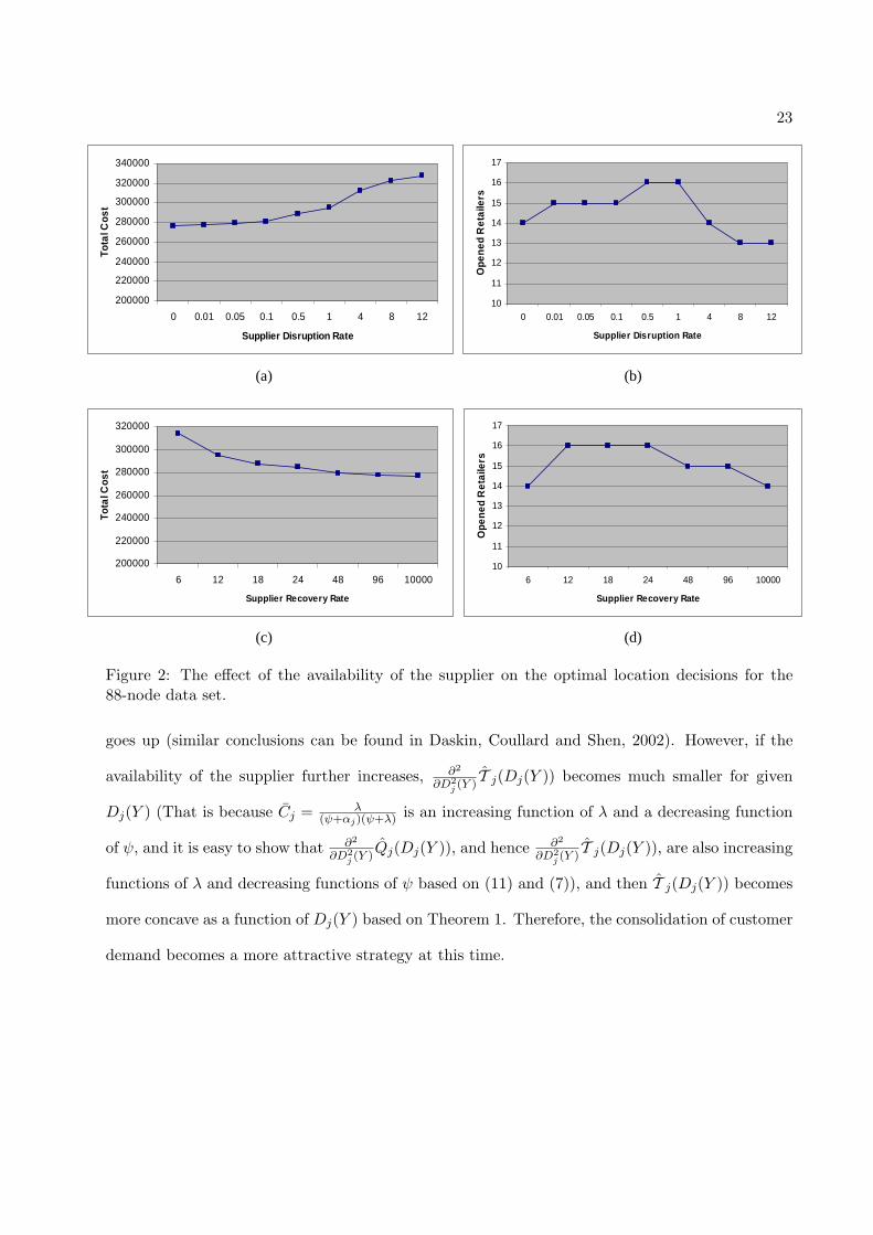
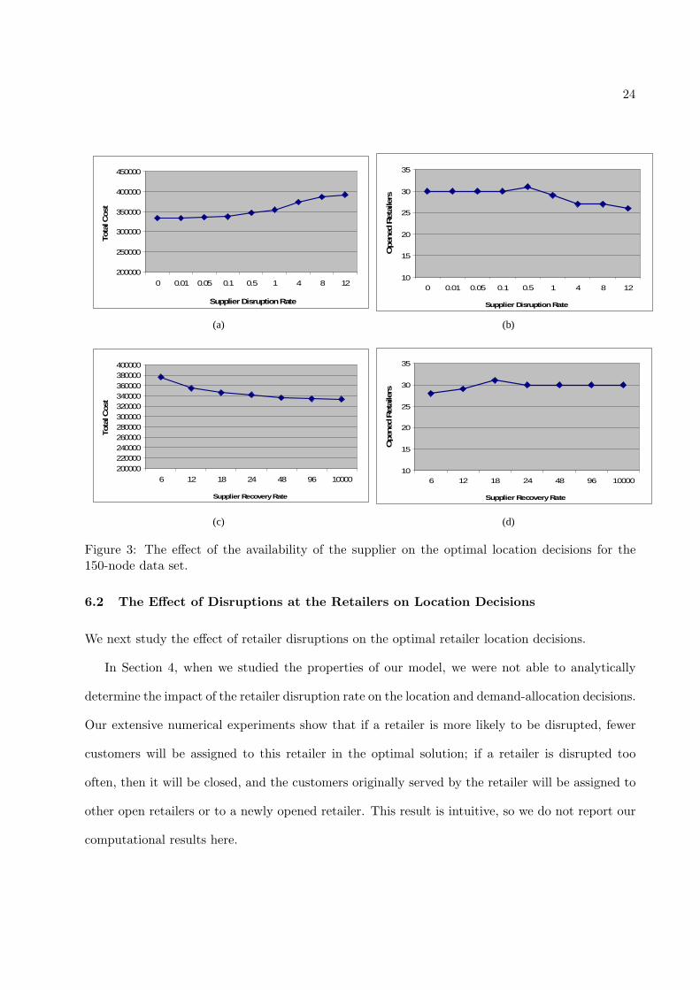
Figures 2 and 3 plot the results in Table 2 graphically, illustrating the relationships between:

• the optimal total cost and the supplier disruption rate,

22

Table 2: The effect of the availability of the supplier on the optimal location decisions.

# of # of Opened # of # of Openedλ ψ Nodes Total Cost Retailers Nodes Total Cost Retailers0 12 88 276767.08 14 150 333286.37 30

0.01 12 277286.85 15 333834.36 300.05 12 278954.51 15 335607.10 300.1 12 280601.75 15 337391.01 300.5 12 288702.56 16 346615.31 31

1 12 294839.21 16 353874.28 294 12 312382.05 14 374168.50 278 12 322345.30 13 385723.81 27

12 12 327646.43 13 392088.10 261 6 88 313632.55 14 150 375981.89 281 12 294839.21 16 353874.28 291 18 287901.07 16 345635.92 311 24 284397.19 16 341599.14 301 48 279499.94 15 336151.49 301 96 277599.60 15 334151.26 301 10000 276767.16 14 333286.46 30

• the optimal number of opened retailers and the supplier disruption rate,

• the optimal total cost and the supplier recovery rate,

• and the optimal number of opened retailers and the supplier recovery rate.

Table 2 and Figures 2 and 3 indicate that the number of opened retailers increases as the avail-

ability of the supplier increases (i.e., λ decreases or ψ increases) and then becomes non-decreasing

as the availability of the supplier further increases. In other words, if the availability of the supplier

increases, the number of opened retailers may increase at the very beginning; however, once this

number decreases, it will never increase again.

An informal explanation of the above observation is as follows.

When the availability of the supplier increases, the working inventory cost at each opened

retailer becomes smaller and relatively unimportant. Therefore, the number of opened retailers

23

200000

220000

240000

260000

280000

300000

320000

340000

0 0.01 0.05 0.1 0.5 1 4 8 12

Supplier Disruption Rate

Tota

l Cos

t

10

11

12

13

14

15

16

17

0 0.01 0.05 0.1 0.5 1 4 8 12


Ope

ned

Ret

aile

rs

200000

220000

240000

260000

280000

300000

320000

6 12 18 24 48 96 10000

Supplier Recovery Rate

Tota

l Cos

t

10

11

12

13

14

15

16

17

6 12 18 24 48 96 10000


Ope

ned

Ret

aile

rs

(a)

(c)

(b)

(d)

Figure 2: The effect of the availability of the supplier on the optimal location decisions for the88-node data set.

goes up (similar conclusions can be found in Daskin, Coullard and Shen, 2002). However, if the

availability of the supplier further increases, ∂2

∂D2j (Y )

T j(Dj(Y )) becomes much smaller for given

Dj(Y ) (That is because Cj = λ(ψ+αj)(ψ+λ) is an increasing function of λ and a decreasing function

of ψ, and it is easy to show that ∂2

∂D2j (Y )

Qj(Dj(Y )), and hence ∂2

∂D2j (Y )

T j(Dj(Y )), are also increasing

functions of λ and decreasing functions of ψ based on (11) and (7)), and then T j(Dj(Y )) becomes

more concave as a function of Dj(Y ) based on Theorem 1. Therefore, the consolidation of customer

demand becomes a more attractive strategy at this time.

24

200000

250000

300000

350000

400000

450000

0 0.01 0.05 0.1 0.5 1 4 8 12


Tota

l Cost

a

10

15

20

25

30

35

0 0.01 0.05 0.1 0.5 1 4 8 12


Open

ed R

etai

lers

a

200000220000240000260000280000300000320000340000360000380000400000

6 12 18 24 48 96 10000


Tota

l Cost

a

(a) (b)

(c) (d)

10

15

20

25

30

35

6 12 18 24 48 96 10000


Ope

ned

Ret

aile

rs

a

Figure 3: The effect of the availability of the supplier on the optimal location decisions for the150-node data set.

6.2 The Effect of Disruptions at the Retailers on Location Decisions

We next study the effect of retailer disruptions on the optimal retailer location decisions.

In Section 4, when we studied the properties of our model, we were not able to analytically

determine the impact of the retailer disruption rate on the location and demand-allocation decisions.

Our extensive numerical experiments show that if a retailer is more likely to be disrupted, fewer

customers will be assigned to this retailer in the optimal solution; if a retailer is disrupted too

often, then it will be closed, and the customers originally served by the retailer will be assigned to

other open retailers or to a newly opened retailer. This result is intuitive, so we do not report our

computational results here.

25

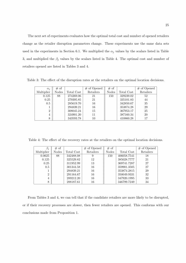
The next set of experiments evaluates how the optimal total cost and number of opened retailers

change as the retailer disruption parameters change. These experiments use the same data sets

used in the experiments in Section 6.1. We multiplied the αj values by the scalars listed in Table

3, and multiplied the βj values by the scalars listed in Table 4. The optimal cost and number of

retailers opened are listed in Tables 3 and 4.

Table 3: The effect of the disruption rates at the retailers on the optimal location decisions.

αj # of # of Opened # of # of OpenedMultiplier Nodes Total Cost Retailers Nodes Total Cost Retailers

0.125 88 274269.06 21 150 329239.02 520.25 279395.85 21 335101.83 440.5 285619.70 16 342850.67 35

1 294839.21 16 353874.28 292 308045.24 15 367953.17 254 324901.20 11 387160.34 208 343593.78 10 410860.28 17

Table 4: The effect of the recovery rates at the retailers on the optimal location decisions.

βj # of # of Opened # of # of OpenedMultiplier Nodes Total Cost Retailers Nodes Total Cost Retailers

0.0625 88 342488.08 9 150 406058.7541 180.125 325529.82 12 385028.7777 210.25 311952.99 13 369741.7287 270.5 301344.58 16 359901.3505 27

1 294839.21 16 353874.2815 292 291164.67 16 350049.9331 324 289212.20 16 347920.1995 338 288187.61 16 346799.7249 34

From Tables 3 and 4, we can tell that if the candidate retailers are more likely to be disrupted,

or if their recovery processes are slower, then fewer retailers are opened. This conforms with our

conclusions made from Proposition 1.

26

6.3 The Benefit of Considering Supply Disruptions in the Supply Chain Design Phase

In this section we compare the performance of the following two supply chain design methods:

• Integrated Approach: consider supply disruptions when we make all supply chain design

decisions including location, demand-assignment and inventory decisions, as we do in this

paper; in other words, design supply chain networks according to the optimal solution to (P).

• Sequential Approach: make location and demand-assignment decisions using the supply chain

design model introduced by Daskin, Coullard, and Shen (2002) without taking supply disrup-

tions into consideration; then at the operational phase, make inventory decisions at opened

retailers using the inventory model proposed by Qi, Shen and Snyder (2007), which considers

supply disruptions.

The integrated approach considers supply disruptions in the supply chain design phase, while

the sequential approach considers supply disruptions only in the operational phase. By comparing

these two methods numerically, we demonstrate the benefit of our integrated model.

We used the same instances as in Section 6.1. For each pair of λ and ψ, and for each data

set (88-node and 150-node), we apply the integrated and sequential approaches to derive the total

costs, which we denote by TCD and TCS , respectively, and then calculate the cost increase for the

sequential approach. As in Tables 2-4, when we calculate the values of TCS and TCD in the tables

below, we add the term π∑

i∈I Di to ensure that TCS and TCD represent the actual total costs.

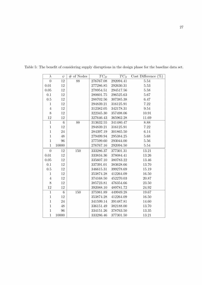
Table 5 lists the costs and cost differences for the baseline data set. It shows that the benefit

of using the integrated approach can be significant—up to 25%—and that the benefit increases as

the supplier disruption rate increases or recovery rate decreases.

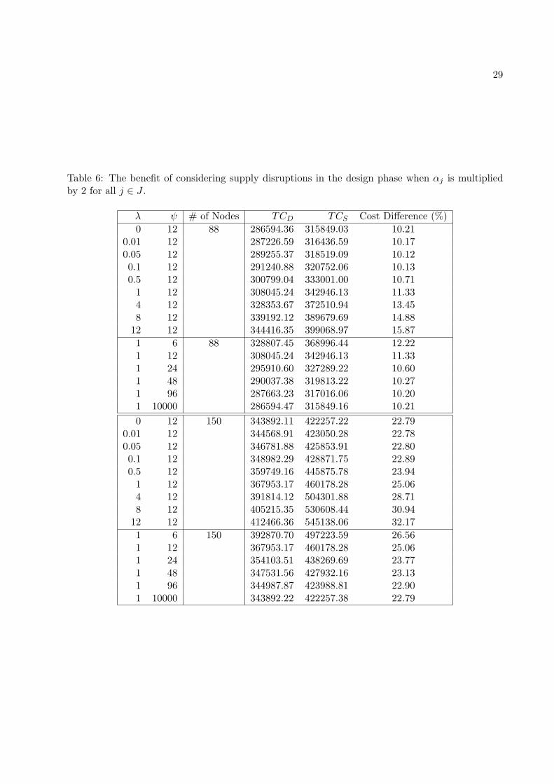
Next, we increased the disruption rates αj at all candidate locations by multiplying them each

by 2 (in Table 6) and 4 (in Table 7). By comparing these two tables with Table 5, we see that

the benefit of using the integrated approach becomes pronounced as the retailer disruption rates

27

Table 5: The benefit of considering supply disruptions in the design phase for the baseline data set.

λ ψ # of Nodes TCD TCS Cost Difference (%)0 12 88 276767.08 292094.41 5.54

0.01 12 277286.85 292630.31 5.530.05 12 278954.51 294517.56 5.580.1 12 280601.75 296525.63 5.670.5 12 288702.56 307385.38 6.47

1 12 294839.21 316125.91 7.224 12 312382.05 342178.31 9.548 12 322345.30 357498.06 10.91

12 12 327646.43 365962.28 11.691 6 88 313632.55 341480.47 8.881 12 294839.21 316125.91 7.221 24 284397.19 301865.50 6.141 48 279499.94 295384.25 5.681 96 277599.60 293044.00 5.561 10000 276767.16 292094.50 5.540 12 150 333286.37 377301.31 13.21

0.01 12 333834.36 378084.41 13.260.05 12 335607.10 380783.22 13.460.1 12 337391.01 383628.66 13.700.5 12 346615.31 399278.69 15.19

1 12 353874.28 412264.09 16.504 12 374168.50 452270.03 20.878 12 385723.81 476354.66 23.50

12 12 392088.10 489781.72 24.921 6 150 375981.89 449949.28 19.671 12 353874.28 412264.09 16.501 24 341599.14 391487.81 14.601 48 336151.49 382188.00 13.701 96 334151.26 378763.50 13.351 10000 333286.46 377301.50 13.21

28

increase, especially if the sequential approach “unluckily” suggests opening retailers at locations

with large disruption rates.

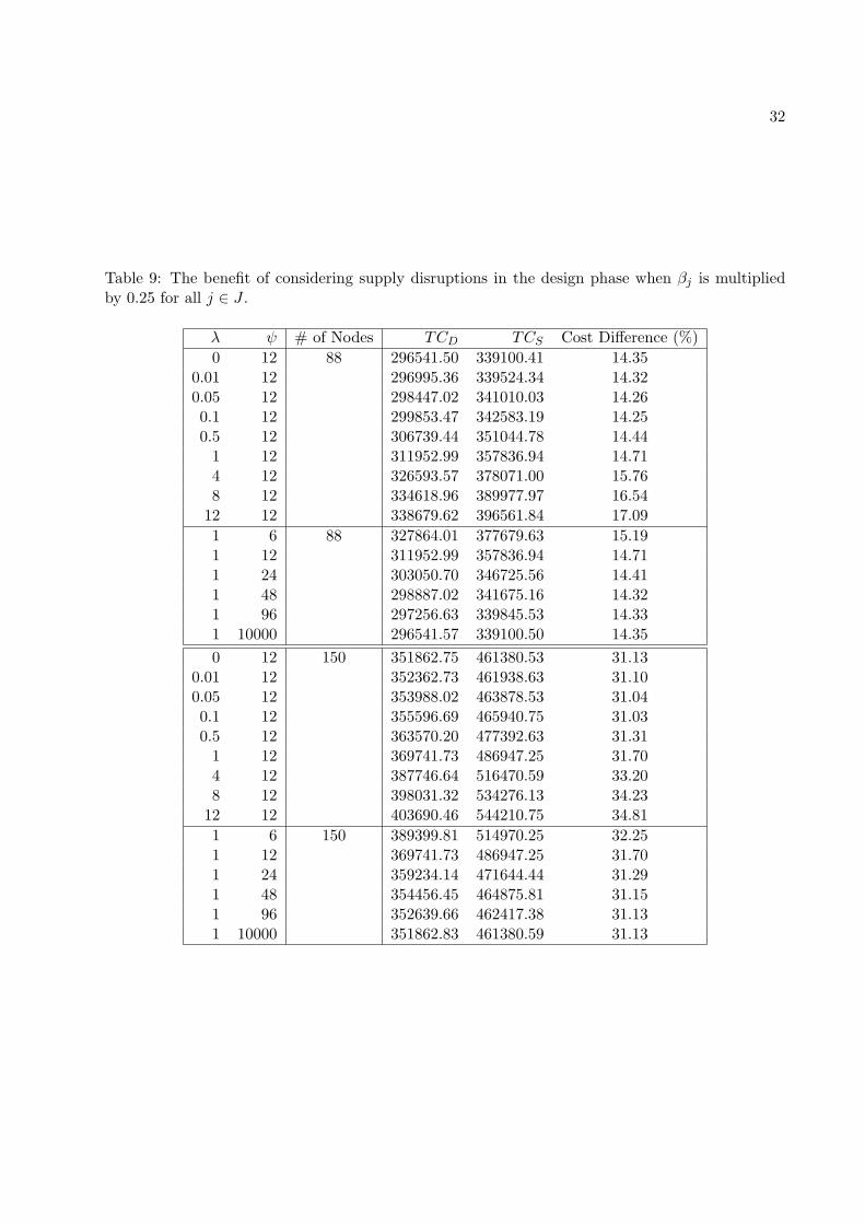
Finally, we decreased the recovery rates βj at all candidate locations by multiplying them each

by 0.5 (in Table 8) and 0.25 (in Table 9). We can see from these two tables that when the recovery

rates at these candidate locations are small, the advantage from using the integrated approach is

significant.

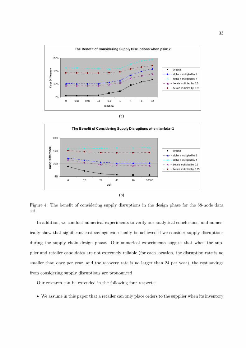
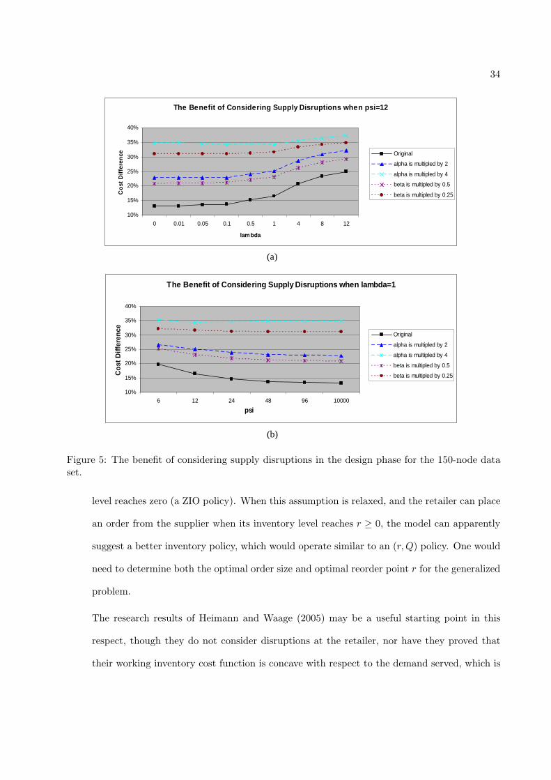
Figures 4 and 5 illustrate the results in Tables 5-9 graphically. For both the 88-node and 150-

node data sets, Figures 4 and 5 show the relationships between the cost savings from considering

supply disruptions in the design phase and the disruption and recovery rates at the retailers and

the supplier.

We conclude that significant cost savings may be realized if disruptions are considered during

the supply chain design phase, especially if the supplier or candidate retailers are often unavailable

(e.g., the disruption rate is at least once per year, and the recovery rate is at most 24 times per

year).

7 Conclusions

We consider an integrated supply chain design problem in which the supplier and retailers are

disrupted randomly. We formulate a nonlinear integer programming model for this problem. An

effective approximation of the objective function of this model is used to make the model easier to

analyze and to solve using a common solution algorithm.

Our analysis leads us to conclude that:

• when the supplier is disrupted more often, or the recovery processes at the supplier or retailer

candidates become slower, it is optimal to serve fewer customers at each opened retailer;

• retailers are more likely to be opened at locations with quick recoveries, and customers are

more likely to be served by retailers with higher recovery rates.

29

Table 6: The benefit of considering supply disruptions in the design phase when αj is multipliedby 2 for all j ∈ J .


0.01 12 287226.59 316436.59 10.170.05 12 289255.37 318519.09 10.120.1 12 291240.88 320752.06 10.130.5 12 300799.04 333001.00 10.71

1 12 308045.24 342946.13 11.334 12 328353.67 372510.94 13.458 12 339192.12 389679.69 14.88

12 12 344416.35 399068.97 15.871 6 88 328807.45 368996.44 12.221 12 308045.24 342946.13 11.331 24 295910.60 327289.22 10.601 48 290037.38 319813.22 10.271 96 287663.23 317016.06 10.201 10000 286594.47 315849.16 10.210 12 150 343892.11 422257.22 22.79

0.01 12 344568.91 423050.28 22.780.05 12 346781.88 425853.91 22.800.1 12 348982.29 428871.75 22.890.5 12 359749.16 445875.78 23.94

1 12 367953.17 460178.28 25.064 12 391814.12 504301.88 28.718 12 405215.35 530608.44 30.94

12 12 412466.36 545138.06 32.171 6 150 392870.70 497223.59 26.561 12 367953.17 460178.28 25.061 24 354103.51 438269.69 23.771 48 347531.56 427932.16 23.131 96 344987.87 423988.81 22.901 10000 343892.22 422257.38 22.79

30

Table 7: The benefit of considering supply disruptions in the design phase when αj is multipliedby 4 for all j ∈ J .


0.01 12 301348.46 350153.75 16.200.05 12 303628.21 352190.53 15.990.1 12 305857.29 354395.09 15.870.5 12 316807.59 366712.66 15.75

1 12 324901.20 376842.47 15.994 12 345745.36 406933.22 17.708 12 356900.87 424181.66 18.85

12 12 362928.64 433510.63 19.451 6 88 345535.10 400484.13 15.901 12 324901.20 376842.47 15.991 24 311433.43 361667.47 16.131 48 304647.89 353958.66 16.191 96 301897.47 350915.13 16.241 10000 300644.11 349584.03 16.280 12 150 358520.40 483347.41 34.82

0.01 12 359311.43 484024.72 34.710.05 12 361898.49 486494.69 34.430.1 12 364477.84 489228.38 34.230.5 12 377327.47 507188.22 34.42

1 12 387160.34 519899.78 34.294 12 414438.52 561427.75 35.478 12 429563.63 586568.63 36.55

12 12 437729.13 600325.44 37.151 6 150 414170.09 560268.13 35.271 12 387160.34 519899.78 34.291 24 370780.98 499115.84 34.611 48 362932.85 489179.38 34.791 96 359860.40 485187.81 34.831 10000 358520.54 483347.63 34.82

31

Table 8: The benefit of considering supply disruptions in the design phase when βj is multipliedby 0.5 for all j ∈ J .


0.01 12 284950.46 311322.28 9.250.05 12 286505.22 313048.94 9.260.1 12 288043.99 314882.63 9.320.5 12 295581.49 324778.13 9.88

1 12 301344.58 332734.13 10.424 12 317831.69 356442.81 12.158 12 327181.71 370388.22 13.21

12 12 332123.32 378095.53 13.841 6 88 319069.47 355875.09 11.541 12 301344.58 332734.13 10.421 24 291579.30 319740.22 9.661 48 287007.03 313834.19 9.351 96 285238.02 311698.75 9.281 10000 284472.90 310831.16 9.270 12 150 340625.69 411817.72 20.90

0.01 12 341150.55 412505.94 20.920.05 12 342873.81 414886.06 21.000.1 12 344598.22 417404.22 21.130.5 12 353280.11 431308.16 22.09

1 12 359901.35 442870.50 23.054 12 379081.51 478535.66 26.248 12 390286.03 500022.28 28.12

12 12 396311.78 512004.84 29.191 6 150 380916.19 476566.25 25.111 12 359901.35 442870.50 23.051 24 348594.86 424363.69 21.741 48 343389.99 416119.50 21.181 96 341447.79 413100.34 20.981 10000 340625.78 411817.81 20.90

32

Table 9: The benefit of considering supply disruptions in the design phase when βj is multipliedby 0.25 for all j ∈ J .


0.01 12 296995.36 339524.34 14.320.05 12 298447.02 341010.03 14.260.1 12 299853.47 342583.19 14.250.5 12 306739.44 351044.78 14.44

1 12 311952.99 357836.94 14.714 12 326593.57 378071.00 15.768 12 334618.96 389977.97 16.54

12 12 338679.62 396561.84 17.091 6 88 327864.01 377679.63 15.191 12 311952.99 357836.94 14.711 24 303050.70 346725.56 14.411 48 298887.02 341675.16 14.321 96 297256.63 339845.53 14.331 10000 296541.57 339100.50 14.350 12 150 351862.75 461380.53 31.13

0.01 12 352362.73 461938.63 31.100.05 12 353988.02 463878.53 31.040.1 12 355596.69 465940.75 31.030.5 12 363570.20 477392.63 31.31

1 12 369741.73 486947.25 31.704 12 387746.64 516470.59 33.208 12 398031.32 534276.13 34.23

12 12 403690.46 544210.75 34.811 6 150 389399.81 514970.25 32.251 12 369741.73 486947.25 31.701 24 359234.14 471644.44 31.291 48 354456.45 464875.81 31.151 96 352639.66 462417.38 31.131 10000 351862.83 461380.59 31.13

33

The Benefit of Considering Supply Disruptions when psi=12

5%

10%

15%

20%

0 0.01 0.05 0.1 0.5 1 4 8 12

lambda

Co

st D

iffe

ren

ce Original

alpha is multipled by 2


beta is multipled by 0.5


The Benefit of Considering Supply Disruptions when lambda=1

5%

10%

15%

20%

6 12 24 48 96 10000

psi

Co

st D

iffe

ren

ce

Original





(a)

(b)

Figure 4: The benefit of considering supply disruptions in the design phase for the 88-node dataset.

In addition, we conduct numerical experiments to verify our analytical conclusions, and numer-

ically show that significant cost savings can usually be achieved if we consider supply disruptions

during the supply chain design phase. Our numerical experiments suggest that when the sup-

plier and retailer candidates are not extremely reliable (for each location, the disruption rate is no

smaller than once per year, and the recovery rate is no larger than 24 per year), the cost savings

from considering supply disruptions are pronounced.

Our research can be extended in the following four respects:

• We assume in this paper that a retailer can only place orders to the supplier when its inventory

34

The Benefit of Considering Supply Disruptions when psi=12

10%

15%

20%

25%

30%

35%

40%

0 0.01 0.05 0.1 0.5 1 4 8 12

lambda

Co

st D

iffe

ren

ce Original





The Benefit of Considering Supply Disruptions when lambda=1

10%

15%

20%

25%

30%

35%

40%

6 12 24 48 96 10000

psi

Co

st D

iffe

ren

ce

Original





(a)

(b)

Figure 5: The benefit of considering supply disruptions in the design phase for the 150-node dataset.

level reaches zero (a ZIO policy). When this assumption is relaxed, and the retailer can place

an order from the supplier when its inventory level reaches r ≥ 0, the model can apparently

suggest a better inventory policy, which would operate similar to an (r,Q) policy. One would

need to determine both the optimal order size and optimal reorder point r for the generalized

problem.

The research results of Heimann and Waage (2005) may be a useful starting point in this

respect, though they do not consider disruptions at the retailer, nor have they proved that

their working inventory cost function is concave with respect to the demand served, which is

35

an important condition in order to apply the Lagrangian relaxation based solution algorithm

proposed in Section 5.

• Dynamic-sourcing is a topic of our ongoing research—a customer can be temporarily served

by other retailer(s) when its assigned retailer is disrupted or out of stock.

• This paper assumes deterministic yields at the supplier and retailers. Random yield will be

considered in our future research.

• We assume constant customer demand when we formulate the working inventory cost at open

retailers. More general stochastic customer demand is to be incorporated into the model for

realism.

References

[1] A. Barrionuevo and C.H. Deutsch, “A Distribution System Brought to Its Knees”, New York

Times, p. C1, Sep. 1, 2005.

[2] E. Berk and A. Arreola-Risa, Note on “Future Supply Uncertainty in EOQ Models”, Naval

Research Logistics 41, 129-132 (1994).

[3] O. Berman, D. Krass, and M.B.C. Menezes, “Facility Reliability Issues in Network p-median

Problems: Strategic Centralization and Co-location Effects”, Operations Research 55, 332-350

(2007).

[4] R.L. Church and M.P. Scaparra, “Protecting Critical Assets: The r-Interdiction Median Prob-

lem with Fortification”, Geographical Analysis 39, 129-146 (2007).

[5] M.S. Daskin, Network and Discrete Location: Models, Algorithms, and Applications, Wiley,

New York (1995).

36

[6] M.S. Daskin, C. Coullard, and Z.J. Shen, “An Inventory-Location Model: Formulation, So-

lution Algorithm and Computational Results”, Annals of Operations Research 110, 83-106

(2002).

[7] D. Erlenkotter, “A Dual-based Procedure for Uncapacitated Facility Location”, Operations

Research 26, 992-1009 (1978).

[8] M.L. Fisher, “The Lagrangian Relaxation Method for Solving Integer Programming Problems”,

Management Science 27, 1-18 (1981).

[9] S. Greenhouse, “Both Sides See Gains in Deal to End Port Labor Dispute”, New York Times,

A14, Nov. 25, 2002.

[10] D. Gupta, “The (q, r) Inventory System with an Unreliable Supplier”, INFOR 34, 59-76 (1996).

[11] M. Halkias, “Wal-Mart Lets Down Its Guard”, Dallas Morning News (Texas), Sept. 14, 2005.

[12] D. Heimann and F. Waage, “A Closed-Form Non-ZIO Approximation Model for the Supply

Chain with Disruptions”, Submitted for publication (2005).

[13] H. Kim, J.C. Lu, and P.H. Kvam, “Ordering Quantity Decisions Considering Uncertainty in

Supply-Chain Logistics Operations”, Working Paper, Georgia Institute of Technology, Atlanta,

GA, 2005.

[14] M. Parlar and D. Berkin, “Future Supply Uncertainty in EOQ Models”, Naval Research Lo-

gistics 38, 107-121 (1991).

[15] M. Parlar and D. Perry, “Analysis of a (q, r, t) Inventory Policy with Deterministic and

Random Yeilds When Future Supply is Uncertain”, European Journal of Operational Research

84, 431-443 (1995).

37

[16] M. Parlar, “Continuous-review Inventory Problem with Random Supply Interruptions”, Eu-

ropean Journal of Operational Research 99, 366-385 (1997).

[17] L. Qi and Z.M. Shen, “A Supply Chain Design Model with Unreliable Supply”, Naval Research

Logistics 54, 829-844 (2007).

[18] L. Qi, Z.M. Shen, and L.V. Snyder, “A Continuous-Review Inventory Model with Disruptions

at Both Supplier and Retailer”, Submitted to Production and Operations Management, 2007.

[19] M.P. Scaparra and R.L. Church, “A Bilevel Mixed-Integer Program for Critical Infrastructure

Protection Planning”, Computers and Operations Research, forthcoming, 2008.

[20] Z.M. Shen, “Integrated Supply Chain Design Models: A Survey and Future Research Direc-

tions”, Journal of Industrial and Management Optimization 3, 1-27 (2007).

[21] Z.M. Shen, C. Coullard, and M.S. Daskin, “A Joint Location-Inventory Model”, Transportation

Science 37, 40-55 (2003).

[22] Z.M. Shen and L. Qi, “Incorporating Inventory and Routing Costs in Strategic Location Mod-

els”, European Journal of Operational Research 179, 372-389 (2007).

[23] L.V. Snyder, “A Tight Approximation for a Continuous-Review Inventory Model with Supplier

Disruptions”, Submitted for publication, 2005.

[24] L.V. Snyder and M.S. Daskin, “Reliability Models for Facility Location: The Expected Failure

Cost Case”, Transportation Science 39, 400-416 (2005).

[25] L.V. Snyder and M.S. Daskin, “Models for Reliable Supply Chain Network Design,” in Critical

Infrastructure: Reliability and Vulnerability, A.T. Murray and T.H. Grubesic (eds.), Chapter

13, 257-289, Springer-Verlag, Berlin, 2007.

38

[26] L.V. Snyder, M.S. Daskin, and C.P. Teo, “The Stochastic Location Model with Risk Pooling”,

European Journal of Operational Research 179, 1221-1238 (2007).

[27] L.V. Snyder, M.P. Scaparra, M.S. Daskin, and R.L. Church, “Planning for Disruptions in

Supply Chain Networks,” in TutORials in Operations Research, M.P. Johnson, B. Norman,

and N. Secomandi (eds.), Chapter 9, 234-257, INFORMS, Baltimore, MD, 2006.

[28] J. Shu, C.P. Teo, Z.J. Shen, “Stochastic Transportation-inventory Network Design Problem”,

Operations Research 53, 48-60 (2005).

[29] B.T. Tomlin, “On the Value of Mitigation and Contingency Strategies for Managing Supply-

chain Disruption Risks”, Management Science 52, 639-657 (2006).

[30] H. Tuy, S. Ghannadan, A. Migdalas, and P. Varbrand, “A Strongly Polynomial Algorithm for

a Concave Production-Transportation Problem with a Fixed Number of Nonlinear Variables”,

Mathematical Programming 72, 229-258 (1996).

Documents

The Eﬁect of Supply Disruptions on Supply Chain …...Arreola-Risa (1994). His approximate cost function not only is convex but also yields a closed His approximate cost function