Trade Costs, Non-Linear Home Market Effect, andother Thingummies. ∗

Matthieu Crozet† Federico Trionfetti‡

This draft: September, 2005

Preliminary and Incomplete

Abstract

Most of the theoretical and empirical studies on the Home Market Effect(HME) make the assumption of the existence of an ”outside good” that ab-sorbs all trade imbalances and equalizes wages. We study the consequencesthat abandoning this assumption has on the HME and on the SecondaryMagnification Effect. These two effects have been used in the literature asdiscriminating criteria to test trade theories. We find that the HME andthe SME remain valid criteria when the outside good is eliminated but theirmagnitude is attenuated. Further, and more importantly, we find that theshape of the HME is non linear. The non-linearity implies that the HME ismore important for very large and very small countries than for medium sizecountries. The empirical investigation conducted on a data set developed atCEPII and comprising 25 industries, 25 countries and 7 years confirms theattenuation of the HME and its non-linear shape.

Keywords: Test of Trade Theories, Economic Geography.JEL Codes: F1, R3.

∗We are grateful to Thierry Mayer and Soledad Zignago for having kindly provided us withdata. We thank Tommaso Mancini for helpful advices and Rosen Marinov for excellent researchassistance. The first author acknowledges financial support from the ACI - Dynamiques de con-centration des activites economiques dans l’espace mondial and the second author acknowledgesfinancial support from FNS (Swiss National Scientific Foundation).

†TEAM, Universite Paris 1. crozet@univ-paris1.fr‡CEPN Universite Paris 13, GIIS, and CEPII. Trionfet@hei.unige.ch

1

1 INTRODUCTION

Models characterized by the presence of increasing returns and monopolistic compe-

tition typically give rise to what has become known as the Home Market Effect: that

is, the magnification of demand idiosyncrasies on output. The HME is so closely

associated to the presence of increasing returns to scale (IRS) and monopolistic

competition (MC) that it has been used as a discriminating criterion in a novel

approach to tasting trade theory initiated by Davis and Weinstein (1999, 2003).

Since then, as it will be discussed below, further theoretical and empirical research

has explored the robustness and the pervasiveness of the HME under various model

modifications. One assumption common to this literature is that of the presence

of a good freely traded and produced under constant returns to scale (CRS) and

perfect competition (PC). This good is often referred to as the “outside good”, The

presence of the outside good serves two purposes. First, it guarantees factor price

equalization, thereby simplifying grandly the solution of the models. Second, it

absorbs all trade imbalances in the IRS-MC good, thereby permitting international

specialization. A different way of seeing the second point is that the outside good

absorbs all changes in demand for labour caused by the expansion or contraction of

the IRS-MC sector, thereby allowing for the reaction of output to demand in the

latter sector to be more than proportional. The assumption of the existence of a

freely traded CRS-PC good is as much convenient as it is at odds with reality. As

noted by Head and Mayer (2004, p. 2634) when discussing this issue in their com-

prehensive account of this literature:“... the CRS sector probably does not have zero

trade costs or the ability to absorb all trade imbalances.” The inconsistency of the

outside good assumption with reality and the fact that many theoretical models and

empirical tests of theories relay on it raises the key question of whether the HME

survives to the elimination of the outside good and, if it does, how is it affected?

The present paper attempts to answer this question.

We introduce explicitly trade costs in the CRS-PC sector in two of the main

models used in the empirical literature on the HME. We find that, in general, the

HME survives in both models but its average magnitude is attenuated. Only when

trade costs are sufficiently high in the CRS-PC sector, then the HME disappears

in one of the two models considered but not in the other one. More interestingly,

both models predict a non linear relationship between share of output and share

2

of demand in all sectors. In one model the HME is absent when countries are of

similar size but it emerges again when countries are of sufficiently dissimilar size.

This giving rise to a “piecewise HME”. In the other model we find that the HME is

present but very weak when countries are of similar size and it becomes smoothly

stronger when country size differences increase. In conclusion, if these models tell the

truth, we should find a piecewise or smoothly increasing HME in IRS-MC sectors as

countries become more dissimilar. We put this result to empirical verification where

we indeed find that for eleven of the 25 sectors we have the piecewise HME predicted

by the first model while we find the smooth non linearity predicted by the second

model for five sectors. One interesting implication of the piecewise or smooth non

linearity is that the HME is more important for large and small countries than for

medium size countries. A result for which we find empirical evidence by looking at

the structural changes in the HME.

As for the CRS-PC sectors the model shows that the less-than-proportional

relationship between share of output and share of demand survives to the presence of

trade costs in all sectors. This result confirms the theoretical validity of the HME as

a discriminating criterion to test trade theories even in the presence of trade costs in

all sectors. For the CRS-PC sector also, the model predicts a smoothly non-linear or

a piecewise less-than-proportional relationship between share of demand and share

of output. The empirical investigation finds little evidence of sectors exhibiting this

type of relationship.

Finally, we study theoretically the sensitivity of the HME to a change a trade

liberalization. In models where there is a freely traded CRS-PC good, trade liberal-

ization accentuates the HME. This result is known as the “secondary magnification”

effect (SME) and it has been used by Head and Ries (2001) as an additional dis-

criminating criterion. Our theoretical analysis shows that the (SME) remains a

valid discriminating criterion when the outside good is removed from the models.

Unfortunately, our data set does not allow us to put this result to econometric

verification.

3

2 RELATIONSHIP TO THE LITERATURE

In the model structures of Krugman (1980) and Helpman and Krugman (1985) the

HME is a feature of the IRS-MC sectors and not of the CRS-PC sectors. Recent

empirical research has used this discriminating criterion to test the empirical merits

of competing trade theories. In their seminal contributions, Davis and Weinstein

(1999, 2003) find stronger evidence of the HME at the regional level (Davis and

Weinstein 1999) than at the international level (Davis and Weinstein 2003). In

a more recent work, Head and Ries (2001) use both the HME and the SME as

discriminating criteria. They consider a model where, in addition to the outside

good and the IRS-MC goods, there is also a CRS-PC good characterized by National

Product Differentiation (NPD) a la Armington (1969). Such good is produced under

constant returns to scale and perfect competition but consumers perceive national

product differently from foreign product. In their model, the IRS-MC good exhibits

the HME while the NPD good does not. Further, they show that a decline in trade

costs magnifies the HME in the IRS-MC good, this is the SME effect. Conversely, in

the NPD good a decline in trade costs reduces the less-than-proportional relationship

between share of output and share of demand. This difference constitutes a new

discriminating criterion that they utilize in the empirical study. Using data for U.S.

and Canadian manufacturing they find evidence in support of both the IRS-MC and

the NPD market structure depending on wether within or between variations are

considered. Most of the evidence however is in favour of the NPD market structure.

Both model structures used in Davis and Weinstein (1999 and 2003) and in Head

and Ries (2001) assume the existence of an outside good. In this paper we remove

the assumption of the existence of an outside good from both of these models and

study the consequences that this has on the HME. In particular, we study the shape

and magnitude of the HME when this assumption is removed and whether the HME

and the SME remain valid discriminating criteria.

The use of the HME for empirical purposes has stimulated research aimed at

studying its robustness to several modifications to the basic model structure.1

1Other papers in this literature have studied different manifestations of the HME while keepingthe assumption of the existence of an outside good whenever appropriate. Such papers includeLundback and Torstensson (1999), Feenstra, Markusen and Rose (2001), Trionfetti (2001), Weder(2003), Brulhart and Trionfetti (2005).

4

Indeed, the very first robustness check has been done by Davis (1998) who has

shown elegantly and succinctly that in the presence of trade costs in the CRS-PC

good the HME may - though not necessarily does - disappear. The HME disappears

only if trade costs in the CRS-PC good are sufficiently high to impede international

trade in such good. The reason is simple: if there is no international trade in the

CRS-PC good then domestic output must satisfy domestic demand in each country

and the CRS-PC good can no longer absorb trade imbalances coming from the IRS-

MC sector. Therefore, in both goods, each country’s share of output must be in

perfect proportionality with the country’s share of world’s expenditure. But trade

costs in the CRS-PC good need not be high enough to impede trade in this good.

Does the HME survive and what shape does it take when trade costs in the CRS-

PC good are not prohibitive? This question remains not fully answered in Davis

(1998). We fully and explicitly derive the relationship between the share of output

and share of expenditure in such model when trade costs in the CRS-PC good are

not prohibitive. We put our theoretical results to empirical verification.

The HME derived in the two-country model extends to the many-country model

if we assume that countries are equidistant from each other. Taking account of

non-equidistant countries in the model complicates the analysis of HMEs because,

without information on the geographical distribution of the expenditure shocks, it

is impossible to know the total effect of the shock on any of the countries. Behrens

et al. (2004) explore this issue in great detail while keeping the assumption of the

existence of an outside good that equalizes wages and absorbs all trade imbalances.

They find that when countries are not equidistant from each other, the HME may

disappear. We limit our analysis to the two country case but complicate matters

by introducing trade costs in the CRS-PC sector. Ideally, one would like to see

an analysis that takes account of trade costs in CRS-PC and of non-equidistant

countries, but this proves to be beyond mathematical tractability for the time being.

In a comprehensive theoretical investigation Head Mayer and Ries (2002) have

studied the pervasiveness of the HME to a number of different models though keep-

ing the assumption (whenever consistent with the model) of a freely traded CRS-PC

good. Their focus is not on the role of trade costs, rather it is on the validity of the

HME as discriminating criterion when the market structure is modified. An inter-

esting result is that the HME emerges even for homogenous goods traded at costs,

5

namely in the Brander (1981) model. However, the good traded in the Brander

model is produced under economies of scale and Cournot oligopoly, so it is differ-

ent from a CRS-PC good. We limit our attention to two distinct cases of market

structure: CRS-PC and IRS-MC and leave for future research the generalization to

other market structures.

Other papers have addressed the issue of trade costs without, however, focusing

on the shape of the HME or on its validity as a discriminating criterion. Amiti

(1998), among other things, studies how the pattern of specialization and trade

varies with country size when industries have different trade costs. One of the

major finding is that small countries will tend to specialize in lower transport cost

goods. This result is similar to the one found in Davis (1998) where the large country

specializes, if at all, in the high trade costs good. But the two models are hardly

comparable since they differ in various respects. In Amiti, for instance, there is no

CRS-PC good. A similar result is found in Hanson and Xiang (2004) who develop a

model where there is no CRS-PC good and the continuum of IRS-MC goods differ

in terms of elasticity of substitutions and trade costs. Their key result, for which

they find empirical support, is that industries with high transport costs and low

substitution elasticity tend to concentrate in larger countries and industries with

low transport costs and high substitution elasticity tend to concentrate in smaller

countries. Holmes and Stevens (2005) also address the question of trade costs and

production structure. Their main focus is to study how the pattern of trade varies

across industries that differ in technology. For this purpose they develop a model

where there is a range of industries which differ in the minimum efficient scale beyond

which average costs are constant. In their model, entry is at intensive margin (more

firms producing the same variety) rather than at the extensive margin (more single-

variety firms) and trade costs are identical in all sectors. The trade pattern that

emerges from this setting is one where goods with low minimum efficient scale (near

constant returns) are not traded, goods with high and medium minimum efficient

scale are traded but the high minimum efficient scale goods are not produced in

the small country. In a way, this pattern is similar to the one in Davis (1998)

since the “near-CRS-PC” good is not traded. The focus of both Amiti (1998)

and Holmes and Stevens (2005), however, is elsewhere than on the HME. They do

not study the existence and shape of the HME nor they address its validity as a

6

discriminating criterion. Further, neither one of these two works studies the issue

empirically. Hanson and Xiang (2004) also do not address the validity of the HME

as discriminating criterion, indeed there is no alternative to the IRS-MC market

structure in their paper. Their focus is on the trade pattern that results from a

model with many different IRS-MC industries.

The remainder of the paper is as follows section 3 presents the two theoretical

models and their predictions, section 4 presents the empirical results and section 5

concludes. The Appendix section derives mathematically the results of the second

model.

3 THEORY

In this section we study the consequences that introducing trade costs in the CRS-

PC good has on the HME and on the SME. We do so in the two principal models

that have been used to test trade theories relaying on the HME and SME as discrim-

inating criteria. We start with a model where the CRS-PC good is differentiated

by country of production and continue with a model where the CRS-PC good is

internationally homogenous.

3.1 National Product Differentiation in the CRS-PC good.

(Model 1)

In this section we study the relationship between share of output and share of de-

mand in a model where the CRS-PC good is differentiated by country of production

a la Armington (1969). For notational convenience we shall refer to this good as

the CRS-PC-A good. Head and Ries (2001) have shown that this model exhibits

the HME and the SME in the IRS-MC good but not in the CRS-PC-A good and

have used these two discriminating criteria to test trade theories. The version of the

model used in Head and Ries (2001) assumes the presence of an “outside good” in

addition to the CRS-PC-A good and to the IRS-MC good. We use the same model

but we eliminate the outside good and study the robustness of the HME and the

SME criteria to such model modification.

7

3.1.1 The Model

Individuals have the following two-tier utility function: U = MγA1−γ, where M =

N∫

0

(cMk)σ−1

σ dk

σσ−1

is the usual CES aggregate of the N varieties of the IRS-

MC good produced in the world and A =(c

σ−1σ

A1 + cσ−1

σA2

) σσ−1

is the CES aggregate

of the two varieties (domestic and foreign) of the CRS-PC-A good. Good A is

produced under constant returns to scale and perfect competition, there is an infinity

of domestic producers and an infinity of foreign producers, but consumers perceive

the domestic kind of A as different from the foreign kind. Consumers perceive as

identical the output of two producers in the same country. There is, therefore,

product differentiation by country of production. That is, consumers care about

the “made in” label. From utility maximization and aggregation over individual

in the same country we have the following demand functions: mii = p−σMiiP

σ−1Mi γYi

, mji = p−σMjiP

σ−1Mi γYi , aii = p−σ

AiiPσ−1Ai (1− γ) Yi , aji = p−σ

AjiPσ−1Ai (1− γ) Yi; where

mii indicates domestic residents’ demand for any of the domestic varieties of M ,

mji indicates country i’s imports of any of the varieties of M , aii indicates domestic

residents’ demand for the domestic output of A, aij indicates country i’s imports

of A. Yi = wiLi is national income, wi is the wage and Li is country i’s labour

endowment.

We assume that there are iceberg transport costs in both sectors:

τM ∈ (0, 1] in M , (1)

τA ∈ (0, 1] in A, (2)

where τM and τA is the fraction of one unit of good sent that arrives at destina-

tion. It is convenient to compact notation by use the following definitions of fee-ness

of trade: φM ≡ τσ−1M ∈ (0, 1], φA ≡ τσ−1

A ∈ (0, 1].

Production technology of any variety of M exhibits increasing returns to scale.

The labor requirement per q units of output is: LM = F + aMq. The production

technology of A exhibits constant returns to scale. To save notation we assume

that one unit of labor input produces one unit of output of A. Profit maximization

gives the following optimal prices: pAii = wi , pAij = 1τA

pAii , pMii = σσ−1

aMwi ,

8

pMij = 1τM

pii. The zero profit condition gives the optimal size of firms in the M

sector, this is: q1 = q2 = FaM

(σ − 1) ≡ q. Using demand functions and Walras’ law

the equilibrium conditions in the goods market are:

pM11q =p1−σ

M11γw1L1

p1−σM11n1 + φMp1−σ

M22n2

+φMp1−σ

M11γw2L2

φMp1−σM11n1 + p1−σ

M22n2

(3)

pM22q =φMp1−σ

M22γw1L1

p1−σM11n1 + φMp1−σ

M22n2

+p1−σ

M22γw2L2

φMp1−σM11n1 + p1−σ

M22n2

(4)

pA11A1 =p1−σ

A11 (1− γ) w1L1

p1−σA11 + φAp1−σ

A22

+φAp1−σ

A11 (1− γ) w2L2

φAp1−σA11 + p1−σ

A22

(5)

Equilibrium conditions in labor markets are:

L1 = A1 + n1 (F + aMq) (6)

L2 = A2 + n2 (F + aMq) (7)

It is convenient to make use of the following definitions: SN ≡ n1

n1+n2, SA ≡

A1

A1+A2, ω ≡ w1

w2, and SL ≡ L1

L1+L2. The five equations (3)-(7), after replacing in

them the expressions for the optimal prices and size of firms, determine the five

endogenous of the model, namely: n1, n2, A1, A2, and ω. The system does not give

algebraic solutions for the five unknowns. We obtain the results in two ways: first

we study the model analytically by use of the implicit function theorem, second we

explore the model numerically.

3.1.2 Analytic results.

We differentiate the system composed of equations (3)-(7) at the symmetric equi-

librium (SL = 12). The resulting expressions for dSN

dSLand dSA

dSLare long and intricated

and, therefore, not particularly informative. These expressions, however, simplify

grandly if we compute them at φM = φA = φ. Thus, for expositional purposes, all

expressions shown in this sub-section are computed at equal trade costs in all sec-

tors. Naturally, in the numerical exploration of the model we relax this restriction

on trade costs.

9

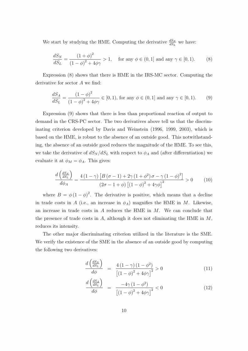
We start by studying the HME. Computing the derivative dSN

dSLwe have:

dSN

dSL

=(1 + φ)2

(1− φ)2 + 4φγ> 1, for any φ ∈ (0, 1] and any γ ∈ [0, 1). (8)

Expression (8) shows that there is HME in the IRS-MC sector. Computing the

derivative for sector A we find:

dSA

dSL

=(1− φ)2

(1− φ)2 + 4φγ∈ [0, 1), for any φ ∈ (0, 1] and any γ ∈ [0, 1). (9)

Expression (9) shows that there is less than proportional reaction of output to

demand in the CRS-PC sector. The two derivatives above tell us that the discrim-

inating criterion developed by Davis and Weinstein (1996, 1999, 2003), which is

based on the HME, is robust to the absence of an outside good. This notwithstand-

ing, the absence of an outside good reduces the magnitude of the HME. To see this,

we take the derivative of dSN/dSL with respect to φA and (after differentiation) we

evaluate it at φM = φA. This gives:

d(

dSN

dSL

)

dφA

=4 (1− γ)

[B (σ − 1) + 2γ (1 + φ2) σ − γ (1− φ)2]

(2σ − 1 + φ)[(1− φ)2 + 4γφ

]2 > 0 (10)

where B = φ (1− φ)2. The derivative is positive, which means that a decline

in trade costs in A (i.e., an increase in φA) magnifies the HME in M . Likewise,

an increase in trade costs in A reduces the HME in M . We can conclude that

the presence of trade costs in A, although it does not eliminating the HME in M ,

reduces its intensity.

The other major discriminating criterion utilized in the literature is the SME.

We verify the existence of the SME in the absence of an outside good by computing

the following two derivatives:

d(

dSN

dSL

)

dφ=

4 (1− γ) (1− φ2)[(1− φ)2 + 4φγ

]2 > 0 (11)

d(

dSA

dSL

)

dφ=

−4γ (1− φ2)[(1− φ)2 + 4φγ

]2 < 0 (12)

10

The sign of (11) and (12) show that a reduction of trade costs in all sectors

magnifies the HME in M while reduces the less than proportional relationship in

A. Therefore, the test developed by Head and Ries (2001), which is based on the

SME, remains valid in the absence of an outside good.

In conclusion - in this model - the two major discriminatory criteria remain

valid when the assumption of the existence of an outside good is removed but their

intensity is attenuated.

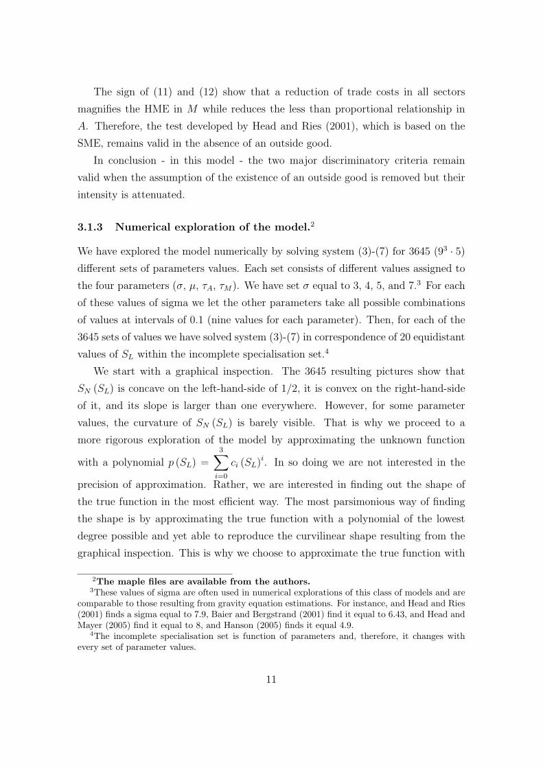
3.1.3 Numerical exploration of the model.2

We have explored the model numerically by solving system (3)-(7) for 3645 (93 · 5)

different sets of parameters values. Each set consists of different values assigned to

the four parameters (σ, µ, τA, τM). We have set σ equal to 3, 4, 5, and 7.3 For each

of these values of sigma we let the other parameters take all possible combinations

of values at intervals of 0.1 (nine values for each parameter). Then, for each of the

3645 sets of values we have solved system (3)-(7) in correspondence of 20 equidistant

values of SL within the incomplete specialisation set.4

We start with a graphical inspection. The 3645 resulting pictures show that

SN (SL) is concave on the left-hand-side of 1/2, it is convex on the right-hand-side

of it, and its slope is larger than one everywhere. However, for some parameter

values, the curvature of SN (SL) is barely visible. That is why we proceed to a

more rigorous exploration of the model by approximating the unknown function

with a polynomial p (SL) =3∑

i=0

ci (SL)i. In so doing we are not interested in the

precision of approximation. Rather, we are interested in finding out the shape of

the true function in the most efficient way. The most parsimonious way of finding

the shape is by approximating the true function with a polynomial of the lowest

degree possible and yet able to reproduce the curvilinear shape resulting from the

graphical inspection. This is why we choose to approximate the true function with

2The maple files are available from the authors.3These values of sigma are often used in numerical explorations of this class of models and are

comparable to those resulting from gravity equation estimations. For instance, and Head and Ries(2001) finds a sigma equal to 7.9, Baier and Bergstrand (2001) find it equal to 6.43, and Head andMayer (2005) find it equal to 8, and Hanson (2005) finds it equal 4.9.

4The incomplete specialisation set is function of parameters and, therefore, it changes withevery set of parameter values.

11

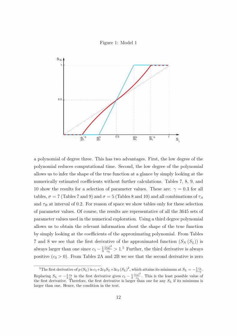
Figure 1: Model 1

1

0.5

S N

0.5 1

SL

S ' is

L Sis

L Sis

L S ' is

L

a polynomial of degree three. This has two advantages. First, the low degree of the

polynomial reduces computational time. Second, the low degree of the polynomial

allows us to infer the shape of the true function at a glance by simply looking at the

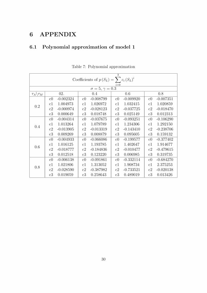
numerically estimated coefficients without further calculations. Tables 7, 8, 9, and

10 show the results for a selection of parameter values. These are: γ = 0.3 for all

tables, σ = 7 (Tables 7 and 9) and σ = 5 (Tables 8 and 10) and all combinations of τA

and τB at interval of 0.2. For reason of space we show tables only for these selection

of parameter values. Of course, the results are representative of all the 3645 sets of

parameter values used in the numerical exploration. Using a third degree polynomial

allows us to obtain the relevant information about the shape of the true function

by simply looking at the coefficients of the approximating polynomial. From Tables

7 and 8 we see that the first derivative of the approximated function (SN (SL)) is

always larger than one since c1− 13

(c2)2

c3> 1.5 Further, the third derivative is always

positive (c3 > 0). From Tables 2A and 2B we see that the second derivative is zero

5The first derivative of p (SL) is c1+2c2SL+3c3 (SL)2, which attains its minimum at SL = − 13

c2c3

.

Replacing SL = − 13

c2c3

in the first derivative gives c1 − 13

(c2)2

c3. This is the least possible value of

the first derivative. Therefore, the first derivative is larger than one for any SL if its minimum islarger than one. Hence, the condition in the text.

12

for values of SL ≈ 1/2. Therefore the true function has the following properties: it

is always increasing, its slope is always larger than 1, it has an inflexion point at

1/2, and it is concave for SL < 1/2 while it is convex for SL > 1/2.

The graphical exploration and the approximation method, obviously, give us the

same results. These results are summarized in Figure 1. The medium-thick straight

line shows the HME in the presence of an outside good (like in Head and Ries, 2001).

Removing the outside good from the model makes the HME non-linear as shown

by the curvilinear shape of the thick line representing the function SN (SL) in the

absence of an outside good. The function is flatter around the symmetric equilibrium

than away from it, implying that the HME is weaker if demand deviations are

concentrated around the mean than if they are more dispersed.

If the model tells the truth, in the data we should find a non-linear relationship

between share of output and share of expenditure of the type shown by the thick

line in Figure 1.

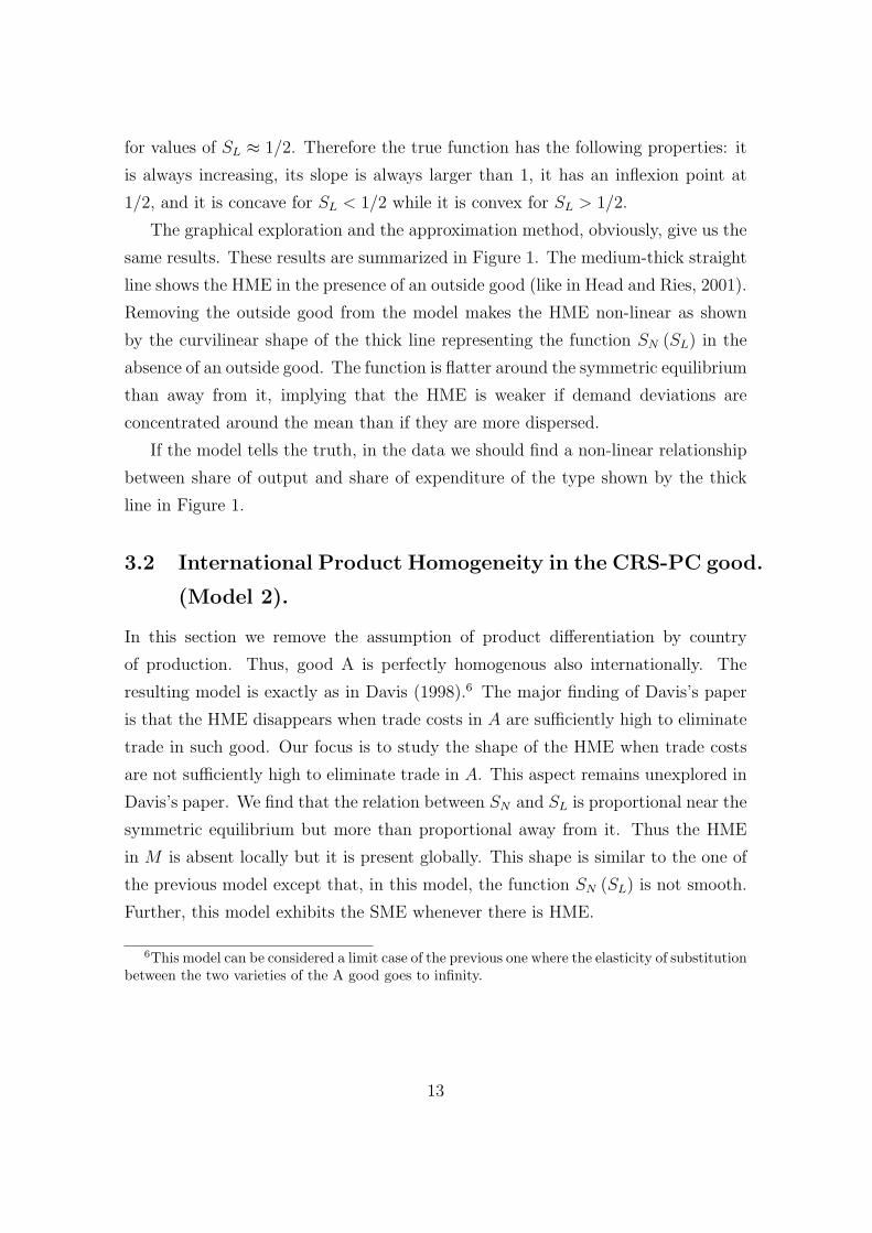
3.2 International Product Homogeneity in the CRS-PC good.

(Model 2).

In this section we remove the assumption of product differentiation by country

of production. Thus, good A is perfectly homogenous also internationally. The

resulting model is exactly as in Davis (1998).6 The major finding of Davis’s paper

is that the HME disappears when trade costs in A are sufficiently high to eliminate

trade in such good. Our focus is to study the shape of the HME when trade costs

are not sufficiently high to eliminate trade in A. This aspect remains unexplored in

Davis’s paper. We find that the relation between SN and SL is proportional near the

symmetric equilibrium but more than proportional away from it. Thus the HME

in M is absent locally but it is present globally. This shape is similar to the one of

the previous model except that, in this model, the function SN (SL) is not smooth.

Further, this model exhibits the SME whenever there is HME.

6This model can be considered a limit case of the previous one where the elasticity of substitutionbetween the two varieties of the A good goes to infinity.

13

3.2.1 The Model

Individual utility function is: U = MγA1−γ, where A is the CRS-PC good and M

is the IRS-MC good. The only difference with the model in the previous section is

that good A is perceived as homogenous regardless of the country of production.

We obtain the results formally in the Appendix section and summarize them here

by use of a Figure.

3.2.2 Results

The HME disappears in this model if there is no trade in A. In the absence of trade

in A, the production of A in each country (A1, and A2) must respond proportionally

to any expenditure shock. Consequently, the response of the output of M in each

country must also be perfectly proportional. Trade in A is prevented if trade costs

in A are sufficiently high. Indeed, country 2 will not import good A as long as

pA2 < pA1

τAand country 1 will not import good A as long as pA1 < pA2

τA. Therefore,

there is no trade in A as long as τA < pA1

pA2< τ−1

A . We denote SL and SL the lower and

upper bound of the set of values of SL in correspondence of which pA1

pA2∈ (

τA, τ−1A

).

If SL ∈(SL, SL

), then there is no trade in A and dSN

dSL= dSA

dSL= 1. We refer to the set(

SL, SL

)as the ”no-trade-in-A” set. The set

(SL, SL

)need not to cover the entire

set [0, 1] in which SL can range. If SL ∈(SL, 1

)or SL ∈

(0, SL

), then there is trade

in A and dSN

dSL> 1 (i.e., there is HME).

The existence of the HME in this model then crucially depends on whether the

set(SL, SL

)is a proper subset of [0, 1]. If it is, then there is HME even in the

presence of trade costs in the homogenous sector, if it is not then trade costs in

the homogenous sector eliminate the HME. Whether the set(SL, SL

)is a proper

subset of [0, 1] depends on the size of trade costs in both sectors (see appendix).

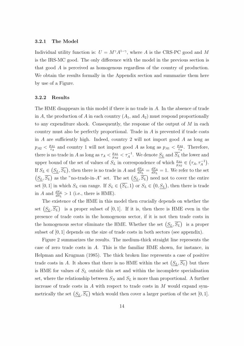
Figure 2 summarizes the results. The medium-thick straight line represents the

case of zero trade costs in A. This is the familiar HME shown, for instance, in

Helpman and Krugman (1985). The thick broken line represents a case of positive

trade costs in A. It shows that there is no HME within the set(SL, SL

)but there

is HME for values of SL outside this set and within the incomplete specialisation

set, where the relationship between SN and SL is more than proportional. A further

increase of trade costs in A with respect to trade costs in M would expand sym-

metrically the set(SL, SL

)which would then cover a larger portion of the set [0, 1].

14

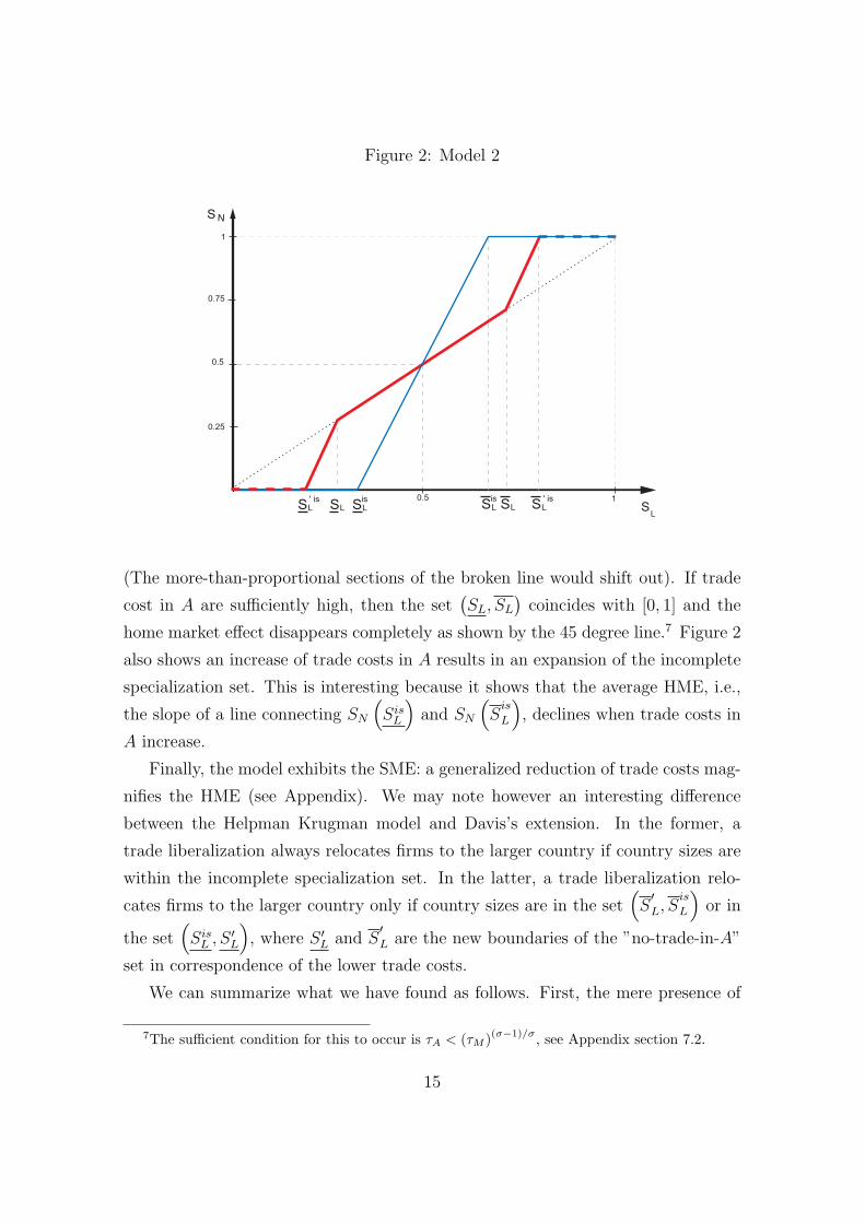
Figure 2: Model 2

1

0.75

0.5

0.25

0.5 1

SL

S N

S ' is

L SL SLSis

L S ' is

LSis

L

(The more-than-proportional sections of the broken line would shift out). If trade

cost in A are sufficiently high, then the set(SL, SL

)coincides with [0, 1] and the

home market effect disappears completely as shown by the 45 degree line.7 Figure 2

also shows an increase of trade costs in A results in an expansion of the incomplete

specialization set. This is interesting because it shows that the average HME, i.e.,

the slope of a line connecting SN

(Sis

L

)and SN

(S

is

L

), declines when trade costs in

A increase.

Finally, the model exhibits the SME: a generalized reduction of trade costs mag-

nifies the HME (see Appendix). We may note however an interesting difference

between the Helpman Krugman model and Davis’s extension. In the former, a

trade liberalization always relocates firms to the larger country if country sizes are

within the incomplete specialization set. In the latter, a trade liberalization relo-

cates firms to the larger country only if country sizes are in the set(S′L, S

is

L

)or in

the set(Sis

L , S ′L), where S ′L and S

′L are the new boundaries of the ”no-trade-in-A”

set in correspondence of the lower trade costs.

We can summarize what we have found as follows. First, the mere presence of

7The sufficient condition for this to occur is τA < (τM )(σ−1)/σ, see Appendix section 7.2.

15

trade costs in every sector does not necessarily eliminate the HME, it only reduces

the average HME. Second, and more importantly, the relationship between share of

demand and share of output is represented by a broken line with a central section

where the HME is absent and a lower and an upper section where there is HME.

We refer to this relationship as the ”piecewise HME”.

3.3 Conclusion to this section.

The two models examined in this section give the same prediction: removing the

outside good makes the HME non linear by either giving it the smooth shape of

model 1 or the piecewise form model 2. If the empirical investigation supports the

non linearity that implies that Davis (1998) point is important, namely, that the

assumption of the existence of an outside good (which is made in virtually all models

of this class) is not an innocuous one. If we find a linear HME instead, than the

outside good assumption, although clearly unrealistic, is innocuous. But the mod-

els give also another prediction: the HME is weak (or absent) near the symmetric

equilibrium than away from it. This means that the HME is more important for

very small and very large countries than for average size countries. If the empiri-

cal investigation supporst this finding then, although the outside good assumption

may not be entirely innocuous, its empirical implications may be of a rather scarce

economic importance for countries of size near the average.

4 EMPIRICAL IMPLEMENTATION.

4.1 Empirical strategy and data

Both models described above give the prediction that the HME is non linear. The

first model exhibits a piecewise HME while the second model exhibits a smooth

non-linearity. To test for the existence of these non-linearity we use the following

equation:

SS,ikt = α1SD,ikt + α2SD,ikt.|SD,ikt|, (13)

16

where i and k denote countries and industries8. SikS and Sik

D are respectively

deviations of production and demand from the average. The estimated values of the

two coefficients α1 and α2 can be associated precisely to different market structure

and HME paradigm, as shown in table (1).

Table 1: Expected coefficient values and associated paradigms

Model 1 Model 2 Unidentified(Smooth HME) (Piecewise HME) (Linear)

IRS-MC α1 > 1, α2 > 0 α1 = 1, α2 > 0 α1 > 1, α2 = 0CRS-PC α1 < 1, α2 < 0 α1 = 1, α2 < 0 α1 < 1, α2 = 0Unidentified - - α1 = 1, α2 = 0

4.1.1 Definition of variables

In the empirical specification we have to take account of the fact that the world

economy consists of R > 2 countries. Denoting with xjkt the quantity produced in

country j, production deviation in country i for product k is:

SS,ikt =xikt∑nj xjkt

− 1

R.

To be consistent with the theoretical predictions we measure SS,ikt in terms of

quantity of output rather than in value. Of course, we do not observe the real

quantities produced in each country. Thus we proxy the quantities by the volume

of production, i.e. xikt = Xikt/pikt, where Xikt is the value of production of good k

in country i and pikt the price of that production.

The variable of demand deviation is defined similarly. It represents the difference

in the quantities demanded that are perceived by producers in a given country i:

SD,ikt =Dikt/pikt∑n

j (Djkt/pjkt)− 1

R,

8The models in previous sections suggest that the relation between demand idiosyncraciesand output is a polynomial of odd order, such as SS,ikt = c1SD,ikt + c2 (SD,ikt)

2 + c3 (SD,ikt)3.

However, such a specification gives rise to multicollinearity among the powered terms. On thecontrary, multicollinearity diagnostics are systematically negative for equation (13).

17

where Dikt is what Davis and Weinstein (2003) call the “Derived Demand” and

Head and Mayer (2004) call the “Nominal Market Potential”. It is the value of

demand emanating from all countries as perceived by producers of k in country i, and

is computed as follows: denoting with Ejk the expenditure on good k in country j

and with Φijkt a measure of all inclusive trade costs, we have: Dikt =∑R

j=1 ΦijktEjk.

An important issue for empirical investigation lies in the measurement of trade

freeness represented by the parameter Φijkt and to which, following Baldwin et al.

(2004) we will refer as the phi-ness of trade. We use here the same estimate of

trade barriers than Head and Ries (2001). Confronting the theoretical demands

expressed on foreign and domestic markets, and assuming symmetric bilateral trade

impediments and free trade within countries, they obtain the following proxy for

Φijkt:

ΦHRijkt =

√zijktzjikt

ziiktzjjkt

,

where zijkt is the value of trade flow of good k, from j to i at year t; it varies

from 0 (prohibitive trade barriers) to 1 (free trade). We use this measure of phi-ness

of trade in the computation of the derived demand9.

This measure of phi-ness of trade has three main qualities. Firstly, ΦHRijkt is time

dependant, so that we can control for the potential changes in access to market

due to trade liberalization processes. Secondly, ΦHRijkt catches all possible sources of

bilateral trade barriers, besides trade frictions associated to geographical distances

and other usual gravity inputs. Thirdly, ΦHRijkt does not impose any strict assumption

on bilateral trade relation and fits similarly to each country-pair. For instance, the

gravity equation assumes a log-linear influence of geographic distance on bilateral

trade and cannot fit well for particularly large or small distances. This is very

important for the purpose of this paper: since we are looking for nonlinearity in the

HME relation, we have to make sure that our measure of access to market does not

introduce a bias that specially affects outlier trading countries.

9Head and Mayer (2004) discuss further this index that they call φ. See also Behrens et al.(2004).

18

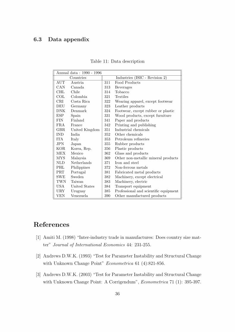
4.1.2 Data

The empirical investigation of the model requires compatible data of production and

demand for a large set of countries and industries. Moreover, we need the bilateral

trade data for the corresponding products and countries in order to compute ΦHRijkt.

We use a database developed in CEPII (see Mayer and Zignago, 2005). It com-

piles production and bilateral trade data from various sources. The resulting data-

base covers 26 industries (ISIC-Rev. 2) and a large number of countries over 25

years (1976-2001). However, we had to restrict the data because of numerous miss-

ing values, so that we get finally a balanced data set for 25 countries, 25 industries

and 7 years (1990-1996). A complete description of the data is given in table 11 in

appendix.10

4.2 Econometric results

Econometric estimates of the model are presented in Tables (2) to (5). All regression

use ordinary least squares.

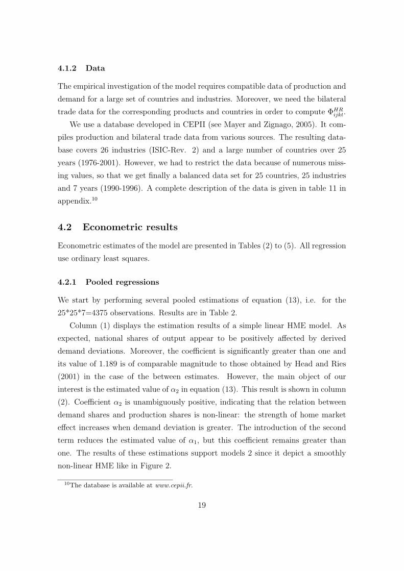
4.2.1 Pooled regressions

We start by performing several pooled estimations of equation (13), i.e. for the

25*25*7=4375 observations. Results are in Table 2.

Column (1) displays the estimation results of a simple linear HME model. As

expected, national shares of output appear to be positively affected by derived

demand deviations. Moreover, the coefficient is significantly greater than one and

its value of 1.189 is of comparable magnitude to those obtained by Head and Ries

(2001) in the case of the between estimates. However, the main object of our

interest is the estimated value of α2 in equation (13). This result is shown in column

(2). Coefficient α2 is unambiguously positive, indicating that the relation between

demand shares and production shares is non-linear: the strength of home market

effect increases when demand deviation is greater. The introduction of the second

term reduces the estimated value of α1, but this coefficient remains greater than

one. The results of these estimations support models 2 since it depict a smoothly

non-linear HME like in Figure 2.

10The database is available at www.cepii.fr.

19

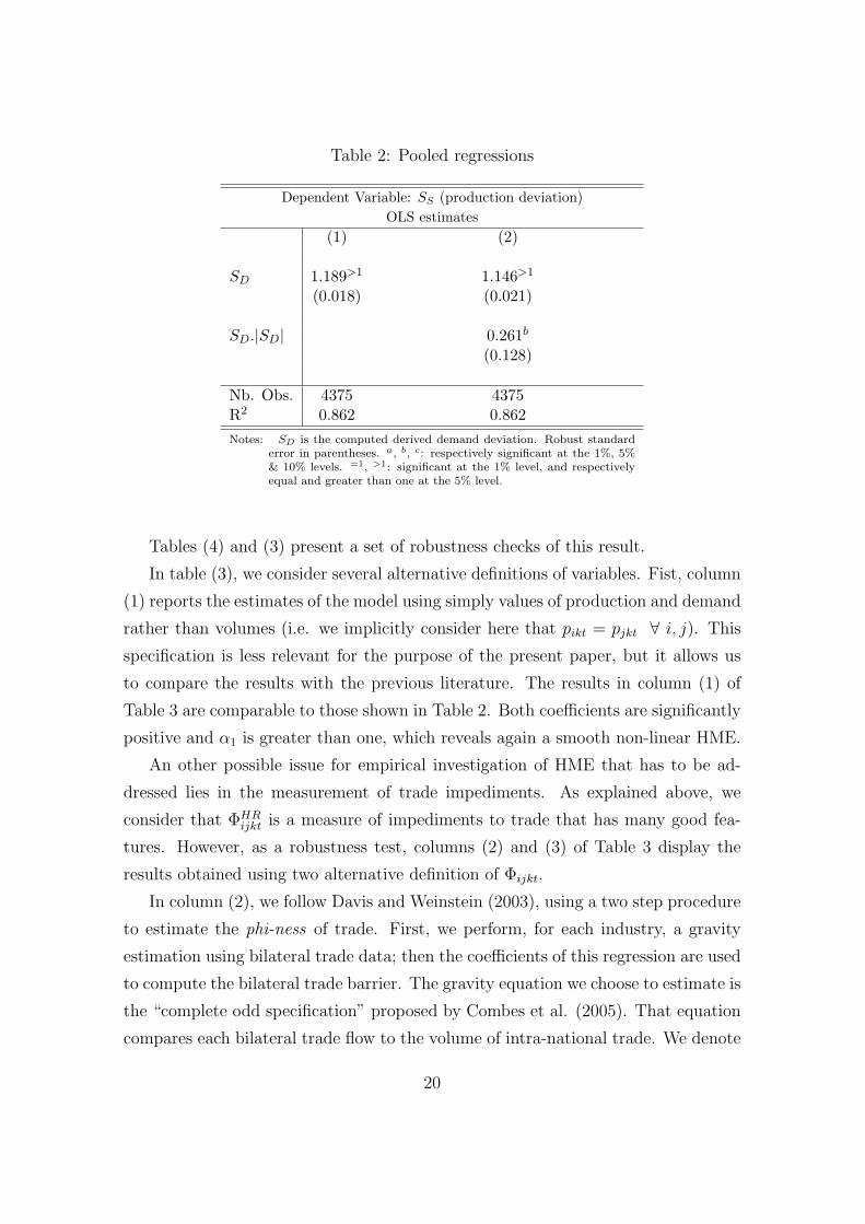
Table 2: Pooled regressions

Dependent Variable: SS (production deviation)OLS estimates

(1) (2)

SD 1.189>1 1.146>1

(0.018) (0.021)

SD.|SD| 0.261b

(0.128)

Nb. Obs. 4375 4375R2 0.862 0.862Notes: SD is the computed derived demand deviation. Robust standard

error in parentheses. a, b, c: respectively significant at the 1%, 5%& 10% levels. =1, >1: significant at the 1% level, and respectivelyequal and greater than one at the 5% level.

Tables (4) and (3) present a set of robustness checks of this result.

In table (3), we consider several alternative definitions of variables. Fist, column

(1) reports the estimates of the model using simply values of production and demand

rather than volumes (i.e. we implicitly consider here that pikt = pjkt ∀ i, j). This

specification is less relevant for the purpose of the present paper, but it allows us

to compare the results with the previous literature. The results in column (1) of

Table 3 are comparable to those shown in Table 2. Both coefficients are significantly

positive and α1 is greater than one, which reveals again a smooth non-linear HME.

An other possible issue for empirical investigation of HME that has to be ad-

dressed lies in the measurement of trade impediments. As explained above, we

consider that ΦHRijkt is a measure of impediments to trade that has many good fea-

tures. However, as a robustness test, columns (2) and (3) of Table 3 display the

results obtained using two alternative definition of Φijkt.

In column (2), we follow Davis and Weinstein (2003), using a two step procedure

to estimate the phi-ness of trade. First, we perform, for each industry, a gravity

estimation using bilateral trade data; then the coefficients of this regression are used

to compute the bilateral trade barrier. The gravity equation we choose to estimate is

the “complete odd specification” proposed by Combes et al. (2005). That equation

compares each bilateral trade flow to the volume of intra-national trade. We denote

20

Table 3: Pooled regressions - Robustness tests

Dependent Variable: SS (production deviation) - OLS estimates(1) (2) (3)

Values Gravity Robust-Φφijk

Market access Market access

SD 1.168>1 1.053>1 1.088>1

(0.021) (0.022) (0.016)

SD.|SD| 0.310b 0.658c 0.189b

(0.133) (0.374) (0.096)

Nb. Obs. 4375 4375 4375R2 0.880 0.507 0.939Notes: SD is the computed derived demand deviation. a, b, c: respec-

tively significant at the 1%, 5% & 10% levels. =1, >1: significantat the 1% level, and respectively equal and greater than one atthe 5% level. Robust standard errors in parentheses.

with zijkt the exports of good k from j to i, xik the production of k in country i, dij

the bilateral distance between countries i and j, Cij a dummy variable that equals

one if countries i and j have a common border. The gravity equation we estimate

is:

ln

(zijkt

mjjkt

)= b1 ln

(Xijkt

Xjjkt

)+ b2 ln

(pijkt

pjjkt

)+ b3 ln

(dij

djj

)+ b4Cij + b5 + εijkt.

In this equation, the estimated value of the intercept (a5) is a measure of the

border effect (b5 < 0). We estimate this equation separately for each industry. All

the coefficients have the expected sign, therefore we can compute a time invariant

gravity-based measure of impediments to trade: ΦGijk =

(d b3k

ij

) (e b4kCij

) (e b5kIntraij

),

where Intraij is a dummy equal to one when i = j.

We then use ΦGijk to compute derived demand and estimate equation (13). The

results shown in column (3) of table (3) are consistent to those obtained with ΦHRijk :

both α1 and α2 are positive and α1 is significantly greater than one, which denotes a

smoothly non-linear HME pattern. However, the overall fit of the model is relatively

weak.

Finally, we consider the possibility that ΦHRijkt may be affected by measurement

21

errors in bilateral trade flows and to sudden changes in prices of traded goods.

Hence, we introduce a third measure of impediments to trade, ΦHRijkt, that is a robust

measure of ΦHRijkt. We estimate the following equation: ln ΦHR

ijkt = εij + εk + εt + νijkt,

where νijkt is an error term and εij, εk and εt are three sets of fixed effects, relative

respectively to each countries pairs, industries and years. Hence, ΦHRijkt is broken up

into three elements. The first one (εij) accounts for the influence of elements such

as distances, bilateral trade agreements and common borders and language. The

second one (εk) accounts for the differences in product transportability. The last

one (εt) captures the evolution of transport techniques and multilateral trade agree-

ments. We define ΦHRijkt as the exponential of the predicted value of this estimation.

As expected, ΦHRijkt is highly correlated to ΦHR

ijkt, but its variance is smaller11. The

estimates of equation (13) using ΦHRijkt are reported in column (3). Once again, we

confirm the results presented in table (2) that show a smoothly non-linear HME

but, as expected, the relation here is less pronounced.

In Table 4 we test whether the result reported in Table 2 is robust to alterna-

tive specifications and country sample. First we ran estimations using a data set

restricted to OECD countries12 (see column 1). When non-OECD countries are ex-

cluded from the data, α2 is non-significant, which gives support to the linear HME

hypothesis. This result suggests that the outside good assumption seems innocuous

if we consider only intra-OECD idyiosincratic demand shocks while it is not if we

consider a larger set of countries.

In column (2) we control for a possible bias resulting from temporary external

imbalances by using the variable TBikt. This variable is computed as the product

of a given country i’s trade balance and the share of i’s production of good k in

the world economy. Controlling for external imbalances does not change the results.

Indeed, it reinforce the smooth non-linearity result since introducing TBikt gives a

smaller α1 and a larger α2.

11Note that even if ΦHRijkt controls for measurement errors that possibly affect ΦHR

ijkt, it may notbe a more accurate measure for the purpose of our empirical work. Indeed, it may reduce theinfluence of some particularly extremes values of ΦHR

ijkt that result from real trade flows. Onceagain, using a measure of access to market that smoothes large deviations may affect seriously theresults.

12Denmark, Spain, Finland, France, United Kingdom, Italy, Japan, Korea, Mexico, The Nether-lands, Philippines, Portugal, Sweden and USA.

22

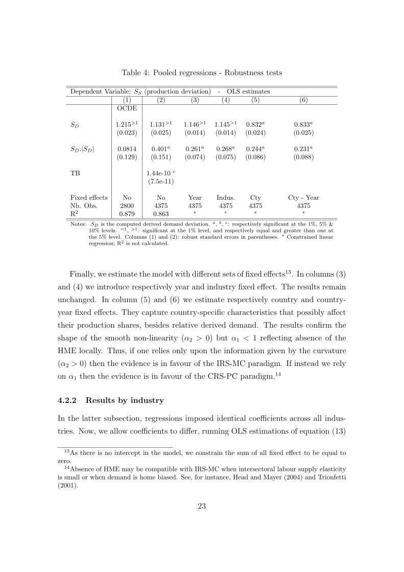
Table 4: Pooled regressions - Robustness tests

Dependent Variable: SS (production deviation) - OLS estimates(1) (2) (3) (4) (5) (6)

OCDE

SD 1.215>1 1.131>1 1.146>1 1.145>1 0.832a 0.833a

(0.023) (0.025) (0.014) (0.014) (0.024) (0.025)

SD.|SD| 0.0814 0.401a 0.261a 0.268a 0.244a 0.231a

(0.129) (0.151) (0.074) (0.075) (0.086) (0.088)

TB 1.44e-10 c

(7.5e-11)

Fixed effects No No Year Indus. Cty Cty - YearNb. Obs. 2800 4375 4375 4375 4375 4375R2 0.879 0.863 ∗ ∗ ∗ ∗

Notes: SD is the computed derived demand deviation. a, b, c: respectively significant at the 1%, 5% &10% levels. =1, >1: significant at the 1% level, and respectively equal and greater than one atthe 5% level. Columns (1) and (2): robust standard errors in parentheses. ∗ Constrained linearregression; R2 is not calculated.

Finally, we estimate the model with different sets of fixed effects13. In columns (3)

and (4) we introduce respectively year and industry fixed effect. The results remain

unchanged. In column (5) and (6) we estimate respectively country and country-

year fixed effects. They capture country-specific characteristics that possibly affect

their production shares, besides relative derived demand. The results confirm the

shape of the smooth non-linearity (α2 > 0) but α1 < 1 reflecting absence of the

HME locally. Thus, if one relies only upon the information given by the curvature

(α2 > 0) then the evidence is in favour of the IRS-MC paradigm. If instead we rely

on α1 then the evidence is in favour of the CRS-PC paradigm.14

4.2.2 Results by industry

In the latter subsection, regressions imposed identical coefficients across all indus-

tries. Now, we allow coefficients to differ, running OLS estimations of equation (13)

13As there is no intercept in the model, we constrain the sum of all fixed effect to be equal tozero.

14Absence of HME may be compatible with IRS-MC when intersectoral labour supply elasticityis small or when demand is home biased. See, for instance, Head and Mayer (2004) and Trionfetti(2001).

23

separately for each industry. The results are summarized in Table 5.

The estimates support the hypothesis that home market effect matters for inter-

national location of industrial production; the relation between demand shares and

market shares is unambiguously more than proportional for 17 industries over the

25 in the sample. As for the shape of the non-linearity, results are more mixed.

Indeed, for 13 industries over 25, α1 ≥ 1 and α2 > 0. Referring to Table

(1), this results is consistent with both the IRS pattern and the hypothesis of the

existence of trade costs in all industries, so that production patterns are shaped

by an non-linear HME. But, for 10 of those sectors, the “Piecewise HME” model

is prevalent. Indeed, those sectors15, the coefficient α1 is not significantly different

from one, while α2 is strictly positive. Therefore, the home market effect hypothesis

is persuasive for these industries, but it really matters only for extreme values of

demand deviations; for most countries, whose world share of derived demand is close

to the mean, a small change in access to market does not involve any magnification

effect on local production. Only 3 sectors are associated with the smooth non-linear

model16. Hence, whereas the pooled regressions provides support to the smooth

HME hypothesis (i.e. model 1), the sectoral analysis gives more evidence in favor

of the piecewise HME (model 2). This conclusion is in line with the theoretical

predictions since the previous sections show that a piecewise HME is more likely to

occur when product differentiation is low.

Further, 5 sectors show a linear HME. For these industries17, α1 > 1 and α2 = 0.

However, the relatively small number of sectors in this case suggests that assuming

free trade in an outside good is not innocuous.

Three sectors do not conform with anyone of the cases in Table 1, but reveals

a positive and non-linear relationship between derived demands and outputs. For

Tobacco, Wearing Apparel and Scientific equipment α1 is smaller than one but α2 is

significantly positive. As explained above, this case may be ascribed to the IRS-MC

paradigm, so that for countries that have a sufficiently high demand deviation, the

non-linear HME is effective in these sectors.

Finally, only 3 sectors (Beverages, Footwear and Other non-metallic products)

15Food, Wood products, Paper, Industrial chemicals, Petroleum Refineries, Glass, Non-ferrousmetal, Electric machinery, Transport equipments and Other manufactured products.

16Printing and publishing, Other chemicals and Non electrical machinery.17Textiles, Rubber products, Iron and steel and Metal products and Plastic.

24

give counter-intuitive results; α1 is greater than one, but α2 is negative.

Overall, the econometric analysis of HME allow to assign almost each industries

to a theoretical paradigm, but results in Table 5 show very little evidence in favor

of the CRS-PC paradigm. The very large number of industries that exhibit a sig-

nificant HME and the 3 puzzling cases, sheds doubt on the possibility of deriving a

clear classification of industrial market structures based on such HME test. How-

ever, leaving aside the idea of providing a robust industrial classification, a very

concordant conclusion arises from the empirical analysis presented in Table 5. We

have clear evidence in favor of the non-linearity of the HME as predicted by the two

models above.

4.2.3 Structural changes in the HME

According to Table 5, ten industries out of 25 show a piecewise HME, i.e. HME is

effective in these industries only for countries in which firms perceive a very large

or a very small share of world demand. In other words, we have found evidence

that in some cases, the HME exists but does not matter for all counties; it has

negligible influence on industrial specialization for countries that have small demand

deviation from the overage, while it has a stronger impact on countries that have a

large demand deviation from the average. In this section, we investigate further this

issue estimating the critical value of demand deviation beyond which HME really

matters.

To do so, we test for parameter structural change in a simple linear HME test.

Hence we perform maximum-Wald tests, estimating the following equation,

SiktS = β1S

iktD (1−Groupπ) + β2S

iktD Groupπ, (14)

where Groupπ is a dummy variable that equals one if SiktD belongs to the π/2

smallest or the π/2 greatest values in the sample and zero otherwise. We test

β1 < β2 performing Wald tests for several values of π, then we consider the larger

value of Wald statistic as the most significant break point18. Hence, the estimated

critical value of π splits the data into three sub-groups: A group of observations that

have small values of derived demand deviations, a group of large derived demand

18See Andrews (1993, 2003).

25

deviations, and a group of intermediate derived demand deviations. The two groups

of extreme values of demand deviations are of identical size and we assume that for

these two groups, HME is of identical magnitude. The smaller is the estimated value

of π the smaller is the size of these two groups of observations. We report in Table

6 the critical value of π and the corresponding regression result.

We first perform this test for the pooled data19. Consistently with the esti-

mations of equation (13) the results show evidence of smooth non-linearity (β2 >

β1 > 1), which suggests that HME matters for all countries. Nevertheless, when we

consider each year successively, we observe a very different result20.

The maximum-Wald test identifies a significant break point for a π ranking from

100 to 148 (i.e. about 20% of the sample). For each year, but 1990 and 1992, this

parameter change has a real economic implication since β2 is greater than one while

β1 does not statistically differ from one. Hence, these estimations suggests that home

market effects only affect industrialization patterns for the first and last decile of

country/industry market-access deviations. For 80% of the countries/industries in

the sample, a better access to market does not lead to any magnification effect on

production.

Results by industry are globally consistent with those displayed in Table 3 21.

For 11 sectors, we observe β1 = 1 and β2 > 1, that is a piecewise HME. For 9

sectors both coefficients are greater than 1, suggesting that HME always matters.

More, for 5 of these the test confirms smooth non-linearity, i.e., β2 > β1 > 1.

Two industries (Apparel and Footwear) give results classifiable under the CRS-PC

paradigm, that is: β1 = 1 and β2 < 1. Finally, six industries show the unexpected

result β1 > β2 ≥ 1. Note however that in all of these industries but beverage, the

critical values of π are very high (greater than 120).

Hence, results in Table 5 confirm those displayed in Table 3 giving support to the

piecewise HME. More, considering each sector separately, the concordance between

the two tables is fairly good: 8 sectors exhibit a piecewise HME in both Table 3 and

Table 5, 2 sectors show a smooth HME, and one a linear HME. Hence, 11 industries

19We increase π from 20 to 2000, using steps of 20 observations.20There are 625 observations for each year. We preform regressions for values of π ranking from

4 to 624, with a step of 4 observations.21There are 175 observations for each of the 25 industries. We perform 42 regression for each

industry with π ranking from 4 to 172 with steps of 4 observations.

26

over 25 are clearly associated to a sigle paradigm exposed in Table 1.

More interestingly, considering the 11 industries that show a piecewise HME in

Table 5, the threshold value of π is always smaller than 36 and its mean is about

22. In other words, that means that in these eleven sectors the HME matters only

for about 12.5% of the observations.

5 CONCLUSION.

We have introduced trade costs in the CRS-PC sector in two of the main model

structures that used the HME and the SME to test trade theory. Our theoretical

results confirm that these criteria are robust to such model modification. However,

when there are trade costs in the CRS-PC good, the HME is attenuated and is non

linear. The non-linearity may take the form of a piecewise function or of a smooth

non-linearity. Our empirical investigation confirms that a significant HME shapes

industrial specialization patterns, at least in a very large majority of sectors. More

importantly, the estimation results strongly support the non-linearity. Considering

an accurate structure of trade costs is important for an understanding of the inter-

national trade and specialization. However, we find a smooth non-linearity in about

5 sectors while in about 11 sectors over 25 we find a piecewise non-linear relation-

ship. In the latter cases, we show that the HME is not significantly effective for a

large fraction of the world economy. In those eleven sectors, HME matters only for

countries that have a very large or a very small deviation of access to market.

27

Table 5: Results by industry

Dependent Variable: SS (production deviation) - OLS estimates311 SD 0.989=1 (0.013) 355 SD 1.234>1 (0.048)Food SD.|SD| 0.493a (0.057) Rubber SD.|SD| -0.265 (0.269)

R2 0.996 products R2 0.950313 SD 1.028>1 (0.007) 356 SD 1.057=1 (0.086)Beverages SD.|SD| -0.159a (0.036) Plastic SD.|SD| 0.277 (0.303)

R2 0.996 products R2 0.942314 SD 0.327a (0.019) 362 SD 1.092=1 (0.051)Tobacco SD.|SD| 1.267a (0.161) Glass and SD.|SD| 1.471=1 (0.292)

R2 0.989 products R2 0.947321 SD 1.343>1 (0.079) 369 SD 1.064>1 (0.011)Textiles SD.|SD| -0.681 (0.421) Other non- SD.|SD| -0.273a (0.092)

R2 0.919 metal. products R2 0.995322 SD 0.787a (0.083) 371 SD 1.142>1 (0.045)Wearing SD.|SD| 0.741b (0.323) Iron and SD.|SD| 0.711 (0.473)Apparel R2 0.956 steel R2 0.967323 SD 1.278>1 (0.106) 372 SD 0.874=1 (0.096)Leather SD.|SD| -1.658 (1.660) Non ferrous SD.|SD| 2.511>1 (0.445)products R2 0.725 metals R2 0.891324 SD 1.379>1 (0.153) 381 SD 1.167>1 (0.026)Footwear SD.|SD| -5.937a (0.894) Metal SD.|SD| 0.195 (0.137)

R2 0.509 products R2 0.977331 SD 0.953=1 (0.024) 382 SD 1.261>1 (0.120)Wood SD.|SD| 0.632a (0.114) Non electric SD.|SD| 2.665>1 (0.729)products R2 0.976 machinery R2 0.892341 SD 1.045=1 (0.025) 383 SD 0.861=1 (0.133)Paper and SD.|SD| 0.643a (0.091) Electric SD.|SD| 5.980>1 (1.201)products R2 0.990 machinery R2 0.841342 SD 1.045>1 (0.005) 384 SD 0.957=1 (0.126)Printing SD.|SD| 0.057a (0.015) Transport SD.|SD| 2.577>1 (0.531)

R2 0.998 equipment R2 0.860351 SD 1.067=1 (0.057) 385 SD 0.363 (0.206)Industrial SD.|SD| 4.324>1 (0.428) Prof. and SD.|SD| 11.614>1 (1.207)chemicals R2 0.952 scientific equip. R2 0.870352 SD 1.144>1 (0.023) 390 SD 0.986=1 (0.141)Other SD.|SD| 0.669a (0.121) Other manuf. SD.|SD| 2.140>1 (0.708)chemicals R2 0.980 Products R2 0.843353 SD 0.974=1 (0.046)Petroleum SD.|SD| 0.774=1 (0.207)refineries R2 0.960Notes: SD is the computed derived demand deviation. a, b, c: respectively significant at the 1%, 5% & 10% levels.

=1, >1: significant at the 1% level, and respectively equal and greater than one at the 5% level. Robuststandard errors in parentheses.

28

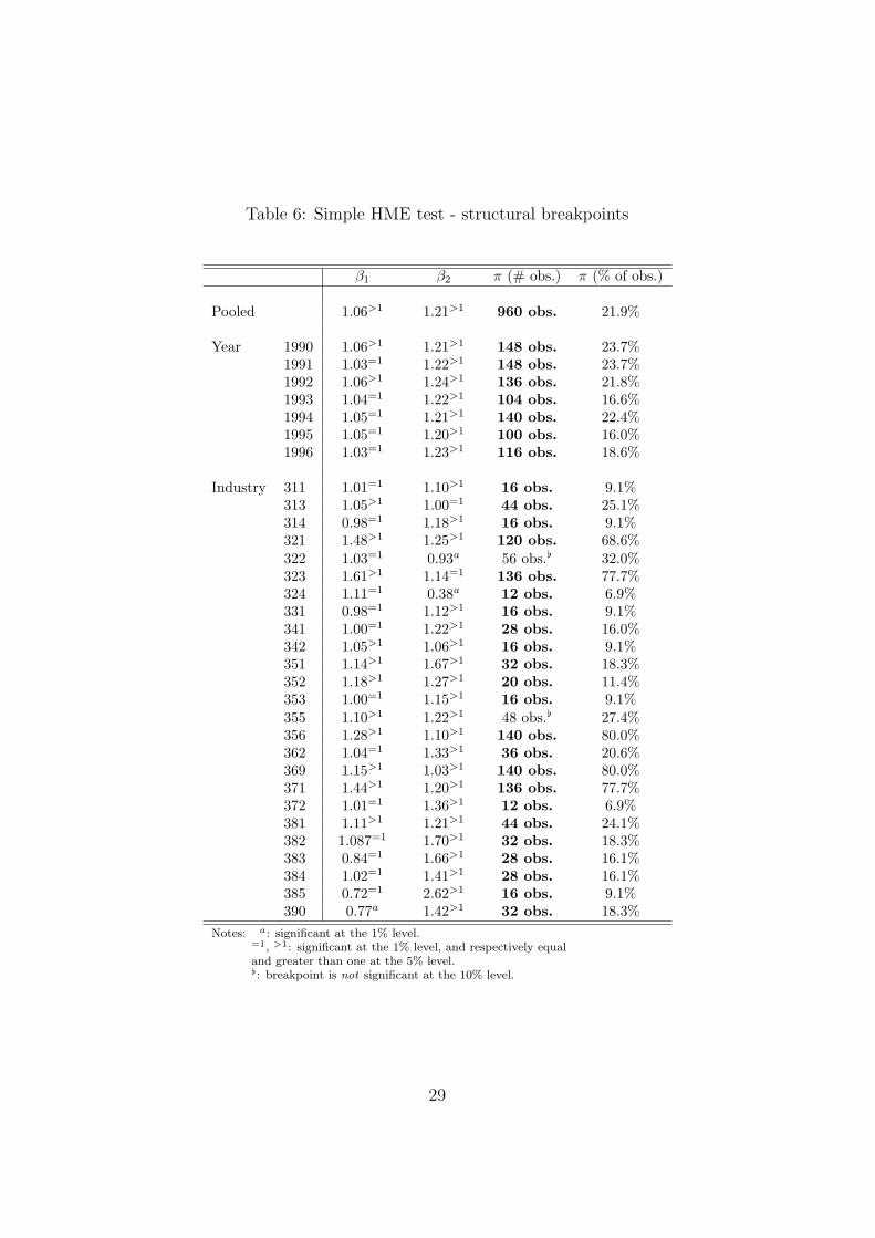
Table 6: Simple HME test - structural breakpoints

β1 β2 π (# obs.) π (% of obs.)

Pooled 1.06>1 1.21>1 960 obs. 21.9%

Year 1990 1.06>1 1.21>1 148 obs. 23.7%1991 1.03=1 1.22>1 148 obs. 23.7%1992 1.06>1 1.24>1 136 obs. 21.8%1993 1.04=1 1.22>1 104 obs. 16.6%1994 1.05=1 1.21>1 140 obs. 22.4%1995 1.05=1 1.20>1 100 obs. 16.0%1996 1.03=1 1.23>1 116 obs. 18.6%

Industry 311 1.01=1 1.10>1 16 obs. 9.1%313 1.05>1 1.00=1 44 obs. 25.1%314 0.98=1 1.18>1 16 obs. 9.1%321 1.48>1 1.25>1 120 obs. 68.6%322 1.03=1 0.93a 56 obs.[ 32.0%323 1.61>1 1.14=1 136 obs. 77.7%324 1.11=1 0.38a 12 obs. 6.9%331 0.98=1 1.12>1 16 obs. 9.1%341 1.00=1 1.22>1 28 obs. 16.0%342 1.05>1 1.06>1 16 obs. 9.1%351 1.14>1 1.67>1 32 obs. 18.3%352 1.18>1 1.27>1 20 obs. 11.4%353 1.00=1 1.15>1 16 obs. 9.1%355 1.10>1 1.22>1 48 obs.[ 27.4%356 1.28>1 1.10>1 140 obs. 80.0%362 1.04=1 1.33>1 36 obs. 20.6%369 1.15>1 1.03>1 140 obs. 80.0%371 1.44>1 1.20>1 136 obs. 77.7%372 1.01=1 1.36>1 12 obs. 6.9%381 1.11>1 1.21>1 44 obs. 24.1%382 1.087=1 1.70>1 32 obs. 18.3%383 0.84=1 1.66>1 28 obs. 16.1%384 1.02=1 1.41>1 28 obs. 16.1%385 0.72=1 2.62>1 16 obs. 9.1%390 0.77a 1.42>1 32 obs. 18.3%

Notes: a: significant at the 1% level.=1, >1: significant at the 1% level, and respectively equaland greater than one at the 5% level.[: breakpoint is not significant at the 10% level.

29

6 APPENDIX

6.1 Polynomial approximation of model 1

Table 7: Polynomial approximation

Coefficients of p (SL) =3∑

i=0

ci (SL)i

σ = 5, γ = 0.3τA\τM 02. 0.4 0.6 0.8

0.2

c0 -0.002324c1 1.004973c2 -0.000974c3 0.000649

c0 -0.008799c1 1.026972c2 -0.028123c3 0.018748

c0 -0.009920c1 1.032415c2 -0.037725c3 0.025149

c0 -0.007351c1 1.020859c2 -0.018470c3 0.012313

0.4

c0 -0.004314c1 1.013264c2 -0.013905c3 0.009269

c0 -0.037675c1 1.079789c2 -0.013319c3 0.008879

c0 -0.093251c1 1.234306c2 -0.143410c3 0.095605

c0 -0.106290c1 1.292150c2 -0.238706c3 0.159132

0.6

c0 -0.004933c1 1.016125c2 -0.018777c3 0.012518

c0 -0.066086c1 1.193785c2 -0.184836c3 0.123220

c0 -0.199577c1 1.402647c2 -0.010477c3 0.006985

c0 -0.377402c1 1.914677c2 -0.479615c3 0.319735

0.8

c0 -0.006138c1 1.021806c2 -0.028590c3 0.019059

c0 -0.091861c1 1.313052c2 -0.387982c3 0.258643

c0 -0.332114c1 1.908734c2 -0.733521c3 0.489019

c0 -0.684270c1 2.375253c2 -0.020138c3 0.013426

30

Table 8: Polynomial approximation

Coefficients of p (SL) =3∑

i=0

ci (SL)i

σ = 7, γ = 0.3τA\τM 02. 0.4 0.6 0.8

0.2

c0 -0.000094c1 1.000206c2 -0.000054c3 0.000036

c0 -0.000434c1 1.001456c2 -0.001763c3 0.001175

c0 -0.000448c1 1.001524c2 -0.001887c3 0.001258

c0 -0.000350c1 1.001074c2 -0.001119c3 0.000746

0.4

c0 -0.000181c1 1.000579c2 -0.000647c3 0.000432

c0 -0.005881c1 1.012993c2 -0.003694c3 0.002463

c0 -0.019885c1 1.056726c2 -0.050866c3 0.033910

c0 -0.021496c1 1.064708c2 -0.065148c3 0.043430

0.6

c0 -0.000191c1 1.000623c2 -0.000723c3 0.000482

c0 -0.011236c1 1.035072c2 -0.037798c3 0.025197

c0 -0.070302c1 1.151020c2 -0.031248c3 0.020832

c0 -0.169397c1 1.430712c2 -0.275752c3 0.183830

0.8

c0 -0.000229c1 1.000803c2 -0.001033c3 0.000688

c0 -0.014432c1 1.050082c2 -0.063650c3 0.042431

c0 -0.138318c1 1.431578c2 -0.464823c3 0.309873

c0 -0.400872c1 1.802177c2 -0.001298c3 0.000866

Table 9: Polynomial approximationInflexion point: values of SL such that p′′ (SL) = 0

σ = 5, γ = 0.3τA\τM 02. 0.4 0.6 0.8

0.2 0.500021 0.500000 0.500000 0.4999990.4 0.500001 0.500000 0.500009 0.5000160.6 0.500025 0.500016 0.499979 0.5000120.8 0.500026 0.500021 0.499995 0.499997

31

Table 10: Polynomial approximationInflexion point: values of SL such that p′′ (SL) = 0

σ = 7, γ = 0.3τA\τM 02. 0.4 0.6 0.8

0.2 0.499903 0.500008 0.500030 0.5000120.4 0.500024 0.500003 0.500013 0.5000200.6 0.500068 0.500021 0.500001 0.5000130.8 0.500038 0.500027 0.500014 0.500019

6.2 Model 2

In this appendix we derive formally the results sketched in Figure 2. Most of these

results do not appear in Davis (1998).

6.2.1 The Model.

Utility maximization gives demand functions for the differentiated commodity iden-

tical to those of the first model in this paper, that is: mii = p−σMiiP

σ−1Mi γYi , mji =

p−σMjiP

σ−1Mi γYi . Since good A is homogenous across countries, consumers have a sin-

gle demand for the good A instead of a demand for each of the country’s variety

of A. This demand is: ai = (1− γ) Yi/pAi , where pAi is the domestic price of A.

Transport costs and technology are the same as in the first model.

When there is trade in A, the equilibrium conditions in the goods market are:

pM11q =p1−σ

M11γ

p1−σM11n1 + φMp1−σ

M22n2

w1L1 +φMp1−σ

M11γ

φMp1−σM11n1 + p1−σ

M22n2

w2L2 (15)

pM22q =φMp1−σ

22 γ

p1−σM11n1 + φMp1−σ

M22n2

w1L1 +p1−σ

22 γ

φMp1−σM11n1 + p1−σ

M22n2

w2L2 (16)

and equilibrium conditions in the labor market are given by:

L1 = A1 + n1 (F + aMq) (17)

L2 = A2 + n2 (F + aMq) (18)

When there is no trade in A, then domestic demand of A must be satisfied by

32

domestic supply. That means Ai = (1− γ) Li. Because of no trade in A, the trade

balance must clear within the IRS-MC good, therefore (by Walras’ law) if any one

of (15) and (16) is satisfied, so is the other one. The market equilibrium equation

for good is then given by any one of (15) and (16) and the market equilibrium

conditions for labour are given by (17) and (18) after replacing Ai = (1− γ) Li in

them.

As explained in the main text, the existence of the HME in this model then

crucially depends on whether the set(SL, SL

)is a proper subset of [0, 1]. If it is,

then there is HME even in the presence of trade costs in the homogenous sector.

If it is not, then trade costs in the homogenous sector eliminate the HME. This is

what we study in the next subsection.

6.2.2 The set(SL, SL

)and the sufficient condition for trade in A.

The share SL takes the value SL when pA1

pA2(= w1

w2) reaches the value 1/τA. Then,

trade in A begins (country 1 starts importing A) and pA1

pA2does not increase any

further. Analogously, SL takes the value SL when the ratio pA1

pA2reaches value τA.

Then, trade in A begins (country 2 starts importing A) and pA1

pA2does not decrease

any further. Substituting pA1

pA2= w1

w2= 1/τA in (15) or (16) and solving for SL gives:

SL =1− τσ

Aτσ−1M

τσ−1A

(τσA − τσ−1

M

)+ 1− τσ

Aτσ−1M

∈[1

2, 1

]if τA > τ

σ−1σ

M . (19)

Analogously, substituting pA1

pA2= τA in (15) or (16) and solving for SL gives:

SL = 1− 1− τσAτσ−1

M

τσ−1A

(τσA − τσ−1

M

)+ 1− τσ

Aτσ−1M

∈[0,

1

2

]if τA > τ

σ−1σ

M . (20)

The strictly sufficient condition for trade in A to exist is easily found by solving

the inequality SL < 1 for τA. This gives the condition: τA > τσ−1

σM , if this condition

is satisfied then there is trade in A.22Naturally, solving SL > 0 gives the same

condition.

22Using the strictly sufficient condition we can compute the tariff equivalent ratio beyond whichthere is no HME. Davis (1998, p.1273), using an overly sufficient conditions, finds that the tariffequivalent in the IRS-MC sector must be 308% higher than in the CRS-PC sector. Using thesufficient condition instead, we obtain a ratio of only 11%.

33

6.2.3 The piecewise relationship between output and demand.

If there is trade in A, then equations (15) and (16) determine n1 and n2 and the

factors market equilibrium equations determine A1 and A2 residually. Assume that

country 1 is the importer of A. Then, pA1

pA2= w1

w2is constant at 1/τA. Substituting

1/τA in the place of pA1

pA2in equations (15) and (16), then solving for n1 and n2 and

rearranging we have.

SN(right) =φ2

M τσ+1A −τAφM+SL(τσ

A−φM+τAφM−φ2M τσ+1

A )τσA−τAφM−φM τ2σ

A +φ2M τσ+1

A +SL(τAφM−φM+φM τ2σA −φM τ2σ−1

A +φ2M τσ−1

A −φ2M τσ+1

A ), for

any SL ∈(SL, S

is

L

).

If we assume that country 1 is the exporter of A than, by replacing pA1

pA2= w1

w2= τA

in equations (15) and (16), solving for n1 and n2 and rearranging we have:

SN(left) = − (−τ2AφM+τAφM−φ2

MφA+τAφM)SL+φ2MφA−τAφM

(φ2MφA+τ2

AφM−τAφM−τ2Aφ2

MφA+τAφMφ2A−φMφ2

A)SL−φ2MφA−τAφA+τAφM+φ2

AφM,for

any SL ∈(Sis

L , SL

).

It is easily verified that, if τA = 1, then SN(rigth) = SN(left) = 1/2+ 1+φM

1−φM

(SL − 1

2

)

exactly as in the benchmark Helpman-Krugman model. To sum up, we have the

following piecewise relationship:

SN =

SN(left), for any SL ∈(Sis

L , SL

)

SL, for any SL ∈ [SL, SL]

SN(right), for any SL ∈(SL, S

is

L

)

The expressions for SA(right) and SA(left) are found analogously. We omit to

report the resulting expressions for reason of space.

6.2.4 The HME and the SME when there is trade in A.

To show the HME it suffices to take the derivatives ofdSN(right)

dSLand

dSN(left)

dSL. They

are:dSN(right)

dSL=

φγ(φγ−φ2θγ2−θ+θ3+φ2θ3γ2−φθ4γ)[(−θ+φγ−φθ2γ2−φ2θγ+φ2θγ2+φθ2)λ−θγ+φθ2γ2−φ2θγ2+φγ]2

,

anddSN(left)

dSL=

φγ(φγ+θ3γ2−φθ4γ−θγ2−φ2θ+φ2θ3)[(θγ2−θγ+φθ2+φ2θγ−φθ2γ2−φ2θ)λ−φθ2+θγ+φ2θ−φγ]2

.

Proving that these derivatives are larger than 1 is a tedious exercise that we omit

here for reason of space. Plotting of the above expressions (like in the figures in the

main text) gives the result at a glance.

To show the SME it suffices to take the derivativesd(SL)

dτA+

d(SL)

dτMand d(SL)

dτA+ d(SL)

dτM.

Computing the first set of derivatives we have:

34

d(SL)

dτA+

d(SL)

dτM= − 2τσ

M(τ3σ+1A −τσ+1

A )(σ−1)

(τσM τσ+1

A −τ2σA τM+τσ

M τσA−τM τA)

2 > 0.

Note that from (20) we have that d(SL)dτA

+ d(SL)dτM

= −(

d(SL)

dτA+

d(SL)

dτM

). Therefore:

d(SL)dτA

+ d(SL)dτM

=2τσ

M(τ3σ+1A −τσ+1

A )(σ−1)

(τσM τσ+1

A −τ2σA τM+τσ

M τσA−τM τA)

2 < 0.

This means that the a trade liberalization in all sectors shrinks the range of

values for which there is no HME. This implies that, for any given country size

above 1/2 for which there is HME, a trade liberalization increases the country’s

share of manufacturing output. Therefore, there is SME.

6.2.5 The incomplete specialization set.

Solving SN(right) = 1 for SL gives us the upper bound of the incomplete specialization

set. This is:

Sis

L =φMτ 1+σ

A − τA

−τA + φ2M − φMτσ

A + φMτσ+1A

∈(

1

2, 1

)if τA > τ

σ−1σ

M . (21)

Analogously, solving SN(left) = 0 for SL gives the lower bound. This is:

SisL = 1− φM τ1+σ

A −τA

−τA+φ2M−φM τσ

A+φM τσ+1A

∈ (0, 1

2

)if τA > τ

σ−1σ

M .

SisL = 1− φMτ 1+σ

A − τA

−τA + φ2M − φMτσ

A + φMτσ+1A

∈(

0,1

2

)if τA > τ

σ−1σ

M . (22)

It is easily checked that the incomplete specialization set coincides with the set [0, 1]

when there is no trade in A. That is: Sis

L = 1 (and SisL = 0) when τA < τ

σ−1σ

M . Also,

it is easily verified that when τA = 1, then we have Sis

L = 11+φM

and SisL = φM

1+φM

exactly as in Helpman and Krugman (1985, section 10.4).

35

6.3 Data appendix

Table 11: Data description

Annual data : 1990 - 1996Countries Industries (ISIC - Revision 2)

AUT Austria 311 Food ProductsCAN Canada 313 BeveragesCHL Chile 314 TobaccoCOL Colombia 321 TextilesCRI Costa Rica 322 Wearing apparel, except footwearDEU Germany 323 Leather productsDNK Denmark 324 Footwear, except rubber or plasticESP Spain 331 Wood products, except furnitureFIN Finland 341 Paper and productsFRA France 342 Printing and publishingGBR United Kingdom 351 Industrial chemicalsIND India 352 Other chemicalsITA Italy 353 Petroleum refineriesJPN Japan 355 Rubber productsKOR Korea, Rep. 356 Plastic productsMEX Mexico 362 Glass and productsMYS Malaysia 369 Other non-metallic mineral productsNLD Netherlands 371 Iron and steelPHL Philippines 372 Non-ferrous metalsPRT Portugal 381 Fabricated metal productsSWE Sweden 382 Machinery, except electricalTWN Taiwan 383 Machinery, electricUSA United States 384 Transport equipmentURY Uruguay 385 Professional and scientific equipmentVEN Venezuela 390 Other manufactured products

References

[1] Amiti M. (1998) “Inter-industry trade in manufactures: Does country size mat-

ter” Journal of International Economics 44: 231-255.

[2] Andrews D.W.K. (1993) “Test for Parameter Instability and Structural Change

with Unknown Change Point” Econometrica 61 (4):821-856.

[3] Andrews D.W.K. (2003) “Test for Parameter Instability and Structural Change

with Unknown Change Point: A Corrigendum”, Econometrica 71 (1): 395-397.

36

[4] Armington, P.S. (1969) “A theory of demand for products distinguished by

place of production” IMF Staff Papers 16: 159-176.

[5] Baldwin, R.E.; Forslid, R.; Martin, Ph.; Ottaviano, G.I.P. and Robert-Nicoud,

F. (2003) Public Policies and Economic Geography. Princeton University Press.

[6] Behrens K., Lamorgese A., Ottaviano G.I.P., Tabuchi T. (2004) “Testing the

‘Home Market Effect’ in a Multi-Country World: A Theory-Based Approach”.

Mimeo.

[7] Baier S.L. and Bergstrand, J.H. (2001) “The Growth of World Trade: Tariffs,

Transport Costs, and Income Similarity”, Journal of International Economics

53(1):1-27.

[8] Brander J. (1981). “Intra-Industry Trade in Identical Commodities” Journal of

International Economics 11: 1-14.

[9] Brulhart M. and F. Trionfetti (2005) “A Test of Trade Theories when Expen-

diture is Home Biased” CEPR working paper 5097.

[10] Combes, P-P. M. Lafourcade, and T. Mayer (2005) ”The trade-creating effects

of business and social networks: evidence from France” Journal of International

Economics 66 (1): 1-29.

[11] Davis, D.R. (1998) “The Home Market, Trade and Industrial Structure” Amer-

ican Economic Review 88, 1264-76.

[12] Davis, D.R., and D.E. Weinstein (1999) “Economic Geography and Regional

Production Structure: an empirical investigation” European Economic Review

43, 379-407.

[13] Davis, D.R., and D.E. Weinstein (2003) “Market Access, Economic Geogra-

phy and Comparative Advantage: an Empirical Test” Journal of International

Economics 59(1):1-23.

[14] Feenstra, R. C., Markusen, J. A. and Rose A.K. (2001) “Using the Gravity

Equation to Differentiate Among Alternative Theories of Trade”. Canadian

Journal of Economics, 34: p 430-47.

37

[15] Hanson H.G., “Market Potential, Increasing Returns, and Geographic Concen-

tration” Journal of International Economics, forthcoming.

[16] Hanson, H.G., and Xiang C. (2004) “The Home Market Effect and Bilateral

Trade Patterns” American Economic Review, 94: 1108-1129.

[17] Head, K., T. Mayer, and J. Ries (2002) “On the Pervasiveness of the Home

Market Effects” Economica 69 (275): 371-390.

[18] Head, K. and T. Mayer (2004) “The Empirics of Agglomeration and Trade”

CEPR WP 3985 and also Ch. 59 in J.V. Henderson and J-F. Thisse (eds),

Handbook of Urban and Regional Economics, Vol. 4. North Holland.

[19] Head, K. and T. Mayer (2004) “Regional Wages and Employment Responses

to Market Potential in the EU” CEPR WP 4908.

[20] Head, K., and J. Ries (2001) “Increasing Returns Versus National Product Dif-

ferentiation as an Explanation for the Pattern of US-Canada Trade” American

Economic Review 91 (4) :858-876.

[21] Holmes, T. J. and J. J. Stevens (2005) “Does home market size matter for the

pattern of trade?” Journal of International Economics 65: 489-505.

[22] Helpman H., and P. Krugman (1985) ”Market Structure and Foreign Trade”,

MIT Press.

[23] Krugman, P.R. (1980) “Scale Economies, Product Differentiation, and the Pat-

tern of Trade” American Economic Review 70, 950-9.

[24] Lundback, E. and J. Torstensson (1998). “Demand Comparative Advantage

And Economic Geography In International Trade: Evidence From The OECD”,

Weltwirtschaftliche Archiv 134 (2): 230-49.

[25] Mayer, T. and S. Zignago (2005) “Market Access in Global and Regional Trade

”CEPII working Paper 2005-02.

[26] Trionfetti, F. (2001) “Using Home-Biased Demand to Test for Trade Theories”

Weltwirtschaftliches Archiv 137 (3): 404-426.

38

[27] Weder, R. (2003) “Comparative Home-Market Advantage: An Empirical

Analysis of British and American Exports”Weltwirtschaftliches Archiv, 139(2):

220-247.

39