The Effect of Service Time Variability on Job Scheduling

Fairness

Eli BroshDepartment of Computer Science

Columbia Universityelibrosh@cs.columbia.edu

Hanoch LevySchool of Computer Science

Tel-Aviv University, Tel-Aviv, Israelhanoch@cs.tau.ac.il

Benjamin Avi-ItzhakRUTCOR, Rutgers University, New Brunswick, NJ, USA

aviitzha@rutcor.rutgers.edu

November 11, 2004

Abstract

Fairness is an inherent and fundamental factor of queue service disciplines in a

large variety of queueing applications, ranging from computer systems, communica-

tions systems and call centers to airport and supermarket waiting lines. Service time

variability across jobs is a major factor affecting both system performance and schedul-

ing rules (for example, computer systems prioritize short jobs over long jobs). Service

time variability and its effects on mean response times have been studied extensively.

However, its effect on queue fairness has not been researched. This work studies the

effect of service time variability on queue fairness. We use the RAQFM queue fairness

measure, whose analysis for the case of the M/M/1 queue was provided in Raz et al.

(2004b), and aim at studying it under a wide variety of service time distributions

(rather than exponential only) with a large range of service time variability. For the

LCFS-PR scheduling we provide a full analysis of the M/G/1 system. We find that

for this system the fairness (when expressed as second moment of discrimination) de-

pends on the first two moments of the service time and only on them. For other service

disciplines (FCFS, LCFS-NPR, ROS-NPR, ROS-PR) we propose to use the common

approach of mapping an arbitrary service time distribution into a Coxian distribu-

tion (via moment mapping) and to use a Markovian-type fairness analysis of RAQFM

for deriving the fairness level of the single server system with Poisson arrivals. The

analysis reveals that queue fairness is sensitive to service time variability and that the

fairness ranking of common scheduling policies (e.g. FCFS, LCFS, ROS) depends on

1

this parameter.

2

1 Introduction

Queueing systems have been used in a wide variety of applications such as computer

systems, call centers, Web services and communications networks, as well as waiting lines

in airports, banks, public offices and others. Queueing Theory has been used for nearly a

century to study the performance of such systems and how to operate them efficiently.

Service times and their distributions play an important role in affecting the perfor-

mance of queueing systems, and the scheduling policies used. One can mention the

Pollaczek-Khinchin formula (see queueing theory text books, e.g. Kleinrock (1975), Cooper

(1981)) where the for the M/G/1 system the average delay is proportional to the second

moment of the service time. Accounting for service times in scheduling policies has been

Widely studied, mainly in the context of optimizing mean system delay or mean delay

cost. A well known result in this context is the so-called µc rule. According to this rule

in a single server system with K classes, if class j incurs cost cj per time unit of wait and

its service time has mean 1/µj , then the cost minimizing rule is to pick for service the

customer with the largest value of µjcj . In other words, the larger the value of µjcj the

higher the priority of this customer (or its class) (see Cox and Smith (1961) Chapter 3.3

and Kleinrock (1976), Lippman (1975)).

Fairness has been recognized as a highly important performance aspect in queues. This

recognition can be found in past studies such as Larson (1987) Rothkopf and Rech (1987)

Palm (1953) Mann (1969) and Whitt (1984). Recent experimental studies of the reaction

of humans to various queue situations (Rafaeli et al. (2002) and Rafaeli et al. (2003)) have

shown that fairness in the queue is very important to humans, perhaps some times even

more than the wait itself. In practice, fairness aspects seem to affect scheduling policies,

in some cases not less than the wish to minimize mean waiting time or weighted mean

wafting time). However, fairness considerations have rarely been expressed quantitatively,

simply since queue fairness quantification was not available until quite recently.

The interest in computer job scheduling and in their fairness has recently raised interest

in quantitatively evaluating queue scheduling fairness. Work in this area has been done

in Avi-Itzhak and Levy (2004), Bender et al. (1998), Bansal and Harchol-Balter (2001),

Wierman and Harchol-Balter (2003), Raz et al. (2004b), Raz et al. (2004a) and Avi-Itzhak

et al. (2004).

Our goal in this work is studying the quantitative effect of service variability on the

3

fairness to jobs in the system and on various common scheduling policies. At the intuitive

level one can easily recognize that high variability may adversely affect queue fairness in

a significant way, since it implies the processing of very long jobs and very short jobs at

the same system. This brings up performance questions as well as operational questions,

such as: 1) To what degree (quantitatively) service time variability affects job scheduling

fairness, 2) How fair are common scheduling disciplines, as a function of the job size

variability, and 3) Which scheduling disciplines achieve higher job fairness (as a function

of the job variability). Since job fairness is one of the major concerns in choosing a

scheduling disciplines, answers to these questions should be useful to system designers

and operators.

To quantify queue fairness we must first select a measure (yarstick) of queue fairness.

To this end, three different approaches have been proposed recently:

1. In Avi-Itzhak and Levy (2004) measures based on order of service have been devised.

2. The slowdown (a.k.a. stretch, normalized response time) was proposed as a metric

of unfairness in several works. In Bender et al. (1998) the max slowdown is used

as indication of unfairness. In Bansal and Harchol-Balter (2001) the max mean

slowdown is used to evaluate the unfairness of the SRPT scheduling policy. In

Wierman and Harchol-Balter (2003), the max mean slowdown is used as a criterion

for evaluating whether a system is fair or unfair.

3. In Raz et al. (2004b) an analysis of the resources allocated by the system to the

various customers forms the base for a fairness measure named Resource Allocation

Queueing Fairness Measure (RAQFM).

As discussed in Avi-Itzhak et al. (2004) the first approach focuses on the relative arrival

times of customers while the second approach focuses on their relative service times; as such

both approaches have difficulties accounting for the tradeoff between relative seniority (the

time spent in the system since arrival) and service requirement. The reader may recognize

this tradeoff and its importance from his/her daily life experience where a very short job

arrives to the queue just shortly after a very long job (e.g in a supermarket), bringing up

the common dilemma of whom it is more fair to serve first.

The third approach (Raz et al. (2004b,a)) focuses on the resources of the system and

their allocation, and thus allows to deal with the tradeoff between service requirement and

4

seniority. The results derived in there show that the measure is indeed sensitive to both

factors and reacts properly (intuitively) in a variety of cases of interest. We will therefore

adopt the RAQFM measure as our fairness evaluation metrics in this study 1

Having selected RAQFM, our first goal is to have an analysis of the fairness of common

service disciplines, under the M/G/1 model. This is required in order to examine systems

under various conditions of service variabilities. To this end, note that the work conducted

on evaluating queue fairness using the RAQFM metric (Raz et al. (2004b,a)) has focused

on exponential service times (M/M/1 model) and therefore, that work needs to be extended

to deal with general service time distribution.

We start by presenting the model and reviewing the RAQFM measure (Section 2). We

then (Section 3) turn to the analysis of the Processor Sharing (PS) and LCFS-Preemptive

disciplines. First (Section 3.1), we recall from the literature that the unfairness of PS

is 0 in all single server systems, including the M/G/1 model (thus it is the most fair

policy), and regardless of service variability. Second (Section 3.2), we start our study

by providing an exact analysis of queue unfairness (expressed as the second moment of

discrimination) in the Last-Come-First-Served Preemptive-Resume (LCFS-PR) M/G/1

system. The analysis leads to a simple numerical recursion for evaluating the individual

discriminations as well as the system’s unfairness in this system. The results derived

imply that system unfairness directly depends on the first two moments of the service

times. That is, service variability is a major factor affecting queue fairness. Further, the

results imply that the system unfairness does not depend on the third and higher moments

of the service time.

We next (Section 4) turn to analyze the First-Come-First-Served (FCFS), LCFS non-

preemptive (LCFS-NPR), Random-Order-of-Service Non-preemptive (ROS-NPR) and ROS-

PR. We realize that the analysis of RAQFM for the M/G/1 model might be quite chal-

lenging. The performance measure of fairness (at least as used in RAQFM) is inherently

more involved (mathematically) than the performance measure of waiting times. This is

so since the latter involves the measures of individual jobs while the former involves a1The reader may question whether the fairness measures developed in the analysis of Weighted Fair

Queueing, like Absolute Fairness Bound and Relative Fairness Bound (see, e.g. Greenberg and Madras

(1992), Keshav (1997), ch. 9 pp. 209-261, Golestani (1994), Zhou and Sethu (2002)) should be considered.

Those measures seem to fit well streams of packets and less so individual jobs, on which our focus is in

this work.

5

comparative measuring between different jobs.

To overcome this difficulty we turn to the common strategy of mapping a general service

time distribution into a Coxian distribution, by matching the moments of the distribu-

tions, and analyzing the Markovian model of with the Coxian service time distribution.

This is done in Section 4 where we first discuss the mapping procedure and then analyze

the corresponding Markovian models. The analysis is carried out via a set of recursive

equations, which can be solved numerically to yield the individual job discrimination as

well as system unfairness.

To provide some insight into the behavior of the non-preemptive policies we provide

in Section 5 an approximate analysis of discrimination in these systems, leading to some

closed form approximate expressions. That analysis demonstrates that in non-preemptive

systems, in the presence of highly variable service times, the positive discrimination expe-

rienced by the long jobs is the dominant factor in the system unfairness.

Lastly (Section 6.1) we turn to conduct a numerical evaluation of the models, examining

their fairness sensitivity to service time variability. The major findings are:

1. Service variability significantly affects the fairness of scheduling policies, including

their relative (fairness) ranking.

2. At high service time variability: At most load conditions the non-preemptive policies

are the most unfair. At high load LCFS-PR is the most unfair. ROS-PR seems to

be the most fair almost at all loads.

3. At low service time variability: At most ranges the policies maintain order of fairness:

FCFS-NPR > ROS-NPR > ROS-PR > LCFS-NPR > LCFS-PR. At very high loads

LCFS-NPR seems to become the most unfair.

2 Model, Notation and Review of RAQFM in a Single Server

System

2.1 Model and Notation

Consider a single server queueing system. The system is subject to a stream of arriving

customers, C1, C2, . . . , arriving at this order. Let ai and ei denote the arrival and exit

(departure) epochs of Ci respectively. Let Si be a random variable denoting the service

requirement (measured in time units) of Ci, where S1, S2, ... are i.i.d as S.Let s(1) = E[S],

6

s(2) = E[S2] σ2S = E[S2]− (E[S])2 and γS = σS/E[S], where γS is called the coefficient of

variation. A specific series of values {ai}Li=1 is called an arrival pattern. A specific series

of values {ai, si}Li=1 is called an arrival and service pattern.

At each epoch t the server grants service at rate xi(t) ≥ 0 to Ci. Let N(t) denote

the number of customers in the system at epoch t. The system is work-conserving, i.e.∫ ei

aixi(t)dt = si. The server has a service rate of one unit and is non-idling, i.e. ∀t,N(t) >

0 ⇒ ∑i xi(t) = 1.

2.2 Individual Customer Discrimination

The fundamental principle underlying RAQFM is the belief that at every epoch t, all

customers present in the system deserve an equal share of the system’s resources. This

principle implies that the share of the server’s resources a customer deserves at t is simply

given by 1/N(t). We call this quantity the momentary warranted service of Ci at epoch t.

Summing this for Ci yields Ridef=

∫ ei

aidt/N(t), the warranted service of Ci. The (overall)

discrimination of Ci, denoted Di is the difference between the warranted service and the

granted service. Since the granted service is Si =∫ ei

aixi(t)dt, then

Di = Si −Ri = Si −∫ ei

ai

dt/N(t). (1)

A positive (negative) value of Di means that a customer receives better (worse) treatment

than it fairly deserves, and therefore it is positively (negatively) discriminated.

Since Di consists of the difference between Si and Ri, we may view Si as the ”positive

discrimination” and denote it by D+i = Si, and Ri as the ”negative discrimination” and

denote it D−i = −Ri. Similarly define D+ and D− to be the steady state limiting values

of D+i and D−

i respectively.

An alternative way to define Di is to define the momentary discrimination of Ci at

epoch t as

δi(t)def= xi(t)− 1/N(t), (2)

and then the overall discrimination of Ci is:

Di =∫ ei

ai

δi(t)dt. (3)

7

An important property of this measure is that it obeys, for every non-idling work-

conserving system, and for every t:∑

i δi(t) = 0, that is, every positive discrimination

is balanced by negative discrimination. This results from the fact that when the system

is non-empty∑

i xi(t) = 1 (due to non-idling) and the overall momentarily warranted

service at such epoch is 1 as well. An important outcome of this property is that if D is

a random variable denoting the discrimination of an arbitrary customer when the system

is in steady state, then E[D] = 0, namely the expected discrimination is zero. The proof

is given in Raz et al. (2004a).

2.3 System Measure of Unfairness

To measure the unfairness of a system, using a particular policy, across all customers, that

is, to measure the system unfairness, one would choose some summary statistics measure

over the values Di, or a function of the distribution of D, where D is a random variable

denoting the discrimination of an arbitrary customer when the system is in steady state.

Since fairness inherently deals with differences in treatment of customers, a natural

choice is the variance of customer discrimination. Since E[D] = 0, this equals the sec-

ond moment and we denote this measure FD2 . Other optional measures are the mean

of distances E[|D|] (denoted F|D|) and the mean negative discrimination −E[D|D < 0]

(denoted FD<0). Throughout this paper, the term “unfairness” refers to FD2 since the

paper focuses on this measure. In some instances we also mention F|D|. FD<0 seems to

be less tractable and is not dealt with in this paper.

3 The Fairness of the PS and the LCFS-PR Scheduling Poli-

cies

3.1 The Fairness of the PS System

The Processor Sharing discipline was analyzed in Raz et al. (2004b) under general assump-

tion of arrival and service times. Under such general processes, which include the M/G/1

case, it was shown that the discrimination of an individual job is identically 0 and so is the

unfairness (expressed either as the second moment of discrimination or as the expected

absolute value of discrimination). As such it is the ”utmost fair” policy. The reader may

verify these results by applying the definitions of discrimination and unfairness given in

Section 2 to the PS discipline.

8

3.2 Analysis of Fairness in the LCFS-PR System

In this section we analyze the fairness and discriminations experienced in the Preemptive

LCFS system. Consider a tagged customer C∗ arriving at the LCFS-PR system. Let

k ≥ 0 be the number of customers it finds upon arrival. C∗ enters service immediately,

and these k customers will remain in the system until C∗ leaves. Recall that S denotes a

random variable representing the service time of C∗, with moments s(1) and s(2).

While C∗ is served, customers arrive at the system at rate λ. Once such a customer

arrives, it preempts C∗, starting a sub-busy-period, at the end of which (after all customers

arriving during the busy period depart, including the preempting one) the service of C∗

resumes. Let N be a random variable denoting the number of arrivals during S; this is

exactly the number of times C∗ will be preempted and a sub-busy-period will start. Since

the arrival process is Poisson, we have:

E[N ] = λE[S]; E[N2] = λ2E[S2] + λE[S]. (4)

Let D|k be a random variable denoting the discrimination experienced by C∗ conditioned

on the number of customers (k) it finds in the system upon arrival. Let D+|k and D−|kbe the conditional positive discrimination (granted service) and negative discrimination

(warranted service). Let DSE |k and DQ|k be the conditional discriminations experienced

by C∗ while in service and while in the queue, respectively. Assuming that the value of S

is s, we have:

DSE |k = (1− 1/k)s, (5)

DQ|k = D1|k + D2|k + ... + DN |k (6)

where Di|k is a random variable denoting the total discrimination experienced by C∗ at the

ith sub-busy period. It is important to note that, while N depends on S, the variables Di|kare i.i.d as D|k (which denotes the discrimination experienced by C∗ during an arbitrary

sub-busy period). The following claim establishes a key relation between the variables

D|k and D|k:

Proposition 3.1. For k = 0, 1, ... the random variable D|k is identical to the variable

D−|k + 1.

Proof. D|k is the discrimination C∗ experiences from the moment a new customer, say C ′,

arrives and until the sub-busy period of C ′ ends. Since during this sub-busy period both

9

C∗ and C ′ are in the system their negative discrimination during this period is identical.

Further, since C ′ sees exactly k+1 customers upon arrival, its discrimination is distributed

as D|k + 1 and its negative discrimination is distributed as D−|k + 1.

Thus, the first and the second moments of D|k are given by:

E[D|k, S = s] = E

[s(1− 1

k + 1) + Y (s, k)

], (7)

E[D2|k, S = s] = E

[s(1− 1

k + 1) + Y (s, k)

]2

(8)

where Y (s, k) =∑N(s)

i=1 Di|k and N(s) is the number of Poisson arrivals in an interval of

length s. Hence

E[Y (s, k) = λsE[D|k]; E[(Y (s, k))2] = λsσD|k + (λ2s2 + λs)E[D|k]2, (9)

where σD|k is the variance of D|k. Taking the expectations of in Eqs. 7 and 8 yields:

E[D|k, S = s] = s

(1− 1

k + 1

)+ λsE[D|k], (10)

and

E[D2|k, S = s] = s2

(1− 1

k + 1

)2

+λE[D2|k] +λ2s2E[D|k]2 +2(

1− 1k + 1

)λs2E[D|k].

(11)

Unconditioning on S = s and using Proposition 3.1 we get

E[D|k] = s(1)

[(1− 1

k + 1) + λE[D−|k + 1

](12)

E[D2|k] = s(2)

(1− 1

k + 1+ λE[D−|k + 1]

)2

+ λs(1)E[(D−)2|k + 1]. (13)

Now, to derive the first two moments of D−|k one can repeat the analysis above only for

the negative part of the discrimination, leading to equations that are similar to Equations

12 and 13:

E[D−|k] = s(1)

[ −1k + 1

+ λE[D−|k + 1]

(14)

10

E[(D−)2|k] = E[S2]( −1

k + 1+ λE[D−|k + 1]

)2

+ λE[S]E[(D−)2|k + 1]. (15)

Equation 14 can be solved by successive substitution to yield:

E[D−|0] = −s(1)∞∑

i=1

ρi−1

i= −s(1)

ρln(1− ρ). (16)

E[D−|k] = − s(1)

ρk+1ln(1− ρ) + s(1)

k∑

i=1

1iρk−i+1

. (17)

Finally, let gk be the probability that C∗ sees k customers upon arrival (which, due

to PASTA, equals the steady state probability of having k customers in the system).

Unconditioning Equation 13 on k we get:

E[D2] = s(2)∞∑

k=0

gk

(1− 1

k + 1+ λE[D−|k + 1]

)2

+ s(1)∞∑

k=0

λgkE[(D−)2|k + 1]. (18)

The LCFS-PR system is a symmetric queue as defined by (Kelly, 1979, Section 3.3).

Therefore2

gk = (1− ρ)ρk, k = 0, 1, 2, ... (19)

where ρ = λE[S]. Thus we have:

E[D2] = s(2)∞∑

k=0

(1− ρ)ρk

(1− 1

k + 1+ λE[D−|k + 1]

)2

+ ρ∞∑

k=0

(1− ρ)ρkE[(D−)2|k + 1].

(20)

Equation 20 demonstrates a direct dependency of the second moment of discrimination

on the first two moments of service time. Further, we may conclude the following important

corollary:

Corollary 3.1. The unfairness of the M/G/1 system with the LCFS-PR service regime,

measured via the RAQFM measure (via the second moment of discrimination) depends on

the first two moments of the service time S, and does not depend on higher moments of

S.2Note that this form results also directly from the following simple argument: In the LCFS-PR iff a

customer leaves behind him k customers he encounters k customers upon arrival. A custoem leaves behind

k + 1 customers iff he preempts a customer who Encountered k upon arrival. Since E[N ] = λE[S] = ρ we

have gk+1 = ρgk implying gk = (1− ρ)ρk, where gk is the probability of encountering k upon arrival.

11

4 Analysis of Non-Preemptive Policies and ROS-Preemptive

under Coxian distribution

In this section we analyze the FCFS, LCFS-NPR, ROS-PR and ROS-NPR policies. The

analysis approach used is to take the (general) distribution of the service time, and ap-

proximate it by a Coxian distribution. This leads to a Markovian model for which the

discrimination and fairness are then derived. For the lack of space we provide only the

analysis of LCFS and ROS-PR. The analysis of the other models can be found in the

appendix.

4.1 Approximating General Service Time distributions by Coxian Dis-

tributions

For the purpose of approximating a general service time distribution we use a second

order moment matching technique (Adan and Resing, 2001, Chapter 2.5). In particular,

we fit a phase-type distribution, either Coxian or Erlangian, on the mean, s(1), and the

coefficient of variation, γS , of the given service time random variable S. We distinguish

between two cases: (a) When 0 < γS < 1 we seek an integer k such that 1k ≈ γS

2, and fit a

k-stage Erlang distribution, Ek, (see Section 4.2) with mean s(1). To match an arbitrary

0 < γS < 1 it is possible to use a more sophisticated distribution such as the mixed Erlang

distribution which selects between Ek and Ek−1 distributions with some fixed probability.

However, using the basic Erlang distribution leads to simpler recurrence equations and

therefore we use it for the analysis. (b) When γS > 1 we use a Coxian-2 distribution

(Adan and Resing, 2001, Chapter 2.4) which is composed of two exponential stages with

mean lengths µi, i = 1, 2 where the move from the first stage to the second one is with

probability p1, and with probability 1 − p1 the service ends after the first stage. For the

approximation we use the following parameters, suggested by Marie (1980):

µ1 = 2s(1), α =0.5γS

, µ2 = µ1α

4.2 Conditional Discrimination in M/Er/1

Consider the M/Er/1 where the service time distribution is Erlang with r exponential

stages. For this distribution the service is assumed to be composed of r phases (i.e.,

stages) arranged serially, where a new customer that enters service proceeds through stages

12

1, . . . , r one at a time; upon completion of the last stage the customer departs. The lengths

of the stages are i.i.d exponentially with parameter rµ.

In a work conserving non-idling M/Er/1 system the time between the arrival of a cus-

tomer and its departure is slotted by arrivals and stage completions. Let Ti, i = 1, 2, . . .

be the duration of the i-th slot, then Ti, i = 1, 2, . . . are i.i.d. random variables exponen-

tially distributed with parameter λ + rµ; the first two moments of Ti are t(1) = 1λ+rµ and

t(2) = 2(λ+rµ)2

= 2(t(1))2. The probabilities that a slot ends with an arrival or with a stage

completion are denoted by λ and µ respectively.

λ =λ

λ + rµ=

ρ

r + ρµ =

rµ

λ + rµ=

r

r + ρ, (21)

where ρ = λ/µ < 1.

The system unfairness, given by E[D2], can be expressed as:

E[D2] = P0E[D2|0, 1] +∞∑

k=1

r∑

j=1

Pk,jE[D2|k, j], (22)

where Pk,j , k ≥ 1 is the probability of finding k customers upon arrival and the served

customer in stage j, P0 = 1−ρ is the probability of finding an empty system, and E[D2|k, j]

is the second moment of D for a customer who arrives to find k customers in the system

and the served one in stage j. Note that Pk,j can be derived numerically via standard

techniques for solving steady state balance equations (see, for example, Kleinrock (1975)).

4.2.1 FCFS

For a tagged customer C residing in the system let a denote the number of customers

ahead of C, let b denote the number of customers behind C, and let j = 1, . . . , r denote

the stage of service in which the served customer is currently found. Such a customer is

said to be in state Sa,b,j . Due to the memoryless properties of the system, the state Sa,b,j

captures all that is needed for predicting the future of C. The momentary discrimination

at state Sa,b,j is independent of the current service stage. We denote it by c(a, b), where

j is omitted.

c(a, b) =

{− 1

a+b+1 a > 01− 1

b+1 a = 0... (23)

13

Let D(a, b, j) denote the accumulated discrimination of C during a walk starting

at state Sa,b,j and ending at the departure of C, and let d(a, b, j)def= d(1)(a, b, j) and

d(2)(a, b, j) be the first and second moments of D(a, b, j). Then

E[D|k, j] = E[d(k, 0, j)] (24)

E[D2|k, j] = E[d(2)(k, 0, j)] (25)

Assume C is in state Sa,b,j . C will encounter one of the two following evens:

1. A new customer arrives into the system. The probability of this event is λ. Afterward

C will move to state Sa,b+1,j .

2. A customer completes its current stage. The probability of this event is µ. If C is

not being served (a 6= 0) it will move to Sa,b,j+1 if j 6= r or to Sa−1,b,j if j = r. If

C is being served (a = 0) it will move to S0,b,j+1 if j 6= r or will leave the system if

j = r.

Thus for customers not in service

D(a, b, j) =

Tc(a, b) + D(a, b + 1, j) w.p λ

T c(a, b) + D(a, b, j + 1) w.p µ, j 6= r

Tc(a, b) + ∆(a > 0)D(a− 1, b, j) w.p µ, j = r

(26)

where T is the duration of the current slot, and ∆() is an indicator function.

Taking expectation leads to the following recursive expression:

d(a, b, j) =

{t(1)c(a, b) + λd(a, b + 1, j) + µd(a, b, j + 1) j 6= r

t(1)c(a, b) + λd(a, b + 1, j) + ∆(a > 0)µd(a− 1, b, 1) j = r(27)

From Eq.(26) for customers not in service

D(a, b, j)2 =

(Tc(a, b) + D(a, b + 1, j))2 w.p λ

(Tc(a, b) + D(a, b, j + 1))2 w.p µ, j 6= r

(Tc(a, b) + ∆(a > 0)D(a− 1, b, 1))2 w.p µ, j = r

(28)

We now take its expectation, after expanding the quadratic terms, and get that

d(2)(a, b, j) = t(2)(c(a, b))2 + λd(2)(a, b + 1, j)+

14

2t(1)c(a, b)λd(a, b + 1, j)+

{µd(2)(a, b, j + 1) + 2t(1)c(a, b)µd(a, b, j + 1)) j 6= r

∆(a > 0)(µd(2)(a− 1, b, j) + 2t(1)c(a, b)µd(a− 1, b, j))) j = r(29)

These recursive relations (equations (29), (27)) combined with equations (24), (23),

(22), (21) can be used, via numerical computation, to derive the system unfairness measure,

V [D].

4.2.2 Preemptive ROS

Consider a preemptive ROS policy in which a preempted customer is immediately se-

lectable for service, i.e., a preempted customer is allowed to immediately reenter service.

Let a =< a1, . . . , ar > be a vector of length r, where ai is the number of customers other

than C that need to complete r − i + 1 stages of service. Let a =∑

i ai denote the total

number of customers in the system other than C. Let c = 1, . . . , r be an integer variable

such that r − c + 1 is the number of stages that C needs to complete. Let s be a boolean

variable which is 1 if C is in service and 0 if it is waiting. The state of C is denoted by

Sa, c, s, j. In this state ai,i = 1, . . . , r customers need to complete r − i + 1 stages, the

tagged customer C needs to complete r − c + 1 stages, the one in service is in its j-th

stage, and it is C if s = 1 and not C if s = 0.

When C is in state Sa,c,s,j it will encounter one of the following possible events:

1. If s = 0 the possible events are:

(a) A customer arrives into the system and C is chosen to receive service next.

The probability of this event is λa+2 and C will move to S<a1+1,...,ar>,c,1,c, where

< a1 + 1, . . . , ar > is the updated vector which includes the additional arriving

customer that needs to complete r stages.

(b) A customer arrives into the system and a waiting customer (other than C) which

is left with r − k + 1 stages is chosen to receive service next. The probability

of this event is λ aka+2 where ak =

{ak k = 2, . . . , r

a1 + 1 k = 1. Then C will move to

S<a1+1,...,ar>,c,0,k.

(c) A customer completes its current stage j, where j 6= r. The probability of this

event is µ and C moves to S<...,aj−1,aj+1+1,...>,c,0,j+1, where < . . . , aj−1, aj+1 +

15

1, . . . > is the updated vector with a single decrease in the number of customers

left with r − j + 1 stages and a single increase in the number of customers left

with r − (j + 1) + 1 stages.

(d) A customer completes service, leaves the system and C is chosen to receive ser-

vice next. The probability of this event is µ/a and C will move to S<a1,...,ar−1>,c,1,c,

where < a1, . . . , ar − 1 > is the updated vector which excludes the departing

customer.

(e) A customer completes service, leaves the system and a waiting customer left

with r − k + 1 stages is chosen to receive service next. The probability of this

event is µaka and C will move to S<a1,...,ar−1>,c,0,k.

2. If s = 1 the possible events are:

(a) Same as (1a)

(b) Same as (1b) but C moves to S<a1+1,...,ar>,j,0,k

(c) Same as (1c) but C moves to Sa,c+1,1,j+1

(d) The customer in service completes its service. The probability of this event is

µ and C leaves the system.

To simplify the recursive equations let a1 + 1def= < a1+1, . . . , ar >, aj − 1, aj+1 + 1

def= <

. . . , aj − 1, aj+1 + 1, . . . >, and ar − 1def= < a1, . . . , ar − 1 >.

For s = 0, d(a, c, s, j) and d(2)(a, c, s, j), can be expressed as

d(a, c, 0, j) = t(1)c(a, s) +λ

a + 2d(a1 + 1, c, 1, c)+

∑

i:ai>0

λai

a + 2d(a1 + 1, c, 0, i)+

{µd(aj − 1, aj+1 + 1, c, 0, j + 1) j 6= rµad(ar − 1, c, 1, c) +

∑i:ai>0 µak

a d(ar − 1, c, 0, i) j = r(30)

d(2)(a, c, 0, j) = t(2)c(a, s)2 +λ

a + 2d(2)(a1 + 1, c, 1, c)+

16

2t(1)c(a, s)λ

a + 2d(a1 + 1, c, 1, c)+

∑

i:ai>0

λai

a + 2d(2)(a1 + 1, c, 0, i)+

2t(1)c(a, s)∑

i:ai>0

λai

a + 2d(a1 + 1, c, 0, i)+

µd(2)(aj − 1, aj+1 + 1, c, 0, j + 1) + 2t(1)c(a, s)µd(aj − 1, aj+1 + 1, c, 0, j + 1) j 6= rµad(2)(ar − 1, c, 1, c) +

∑i:ai>0 µak

a d(2)(ar − 1, c, 0, i)+2t(1)c(a, s)( µ

ad(ar − 1, c, 1, c) +∑

i:ai>0 µaka d(ar − 1, c, 0, i)) j = r

(31)

For s = 1 they are given by

d(a, c, 1, j) = t(1)c(a, s) +λ

a + 2d(a1 + 1, c, 1, c)+

∑

i:ai>0

λai

a + 2d(a1 + 1, j, 0, i)+

{µd(a, c + 1, 1, j + 1) j 6= r

0 j = r(32)

d(2)(a, c, 1, j) = t(2)c(a, s)2 +λ

a + 2d(2)(a1 + 1, c, 1, c)+

2t(1)c(a, s)λ

a + 2d(a1 + 1, c, 1, c)+

∑

i:ai>0

λai

a + 2d(2)(a1 + 1, j, 0, i)+

2t(1)c(a, s)∑

i:ai>0

λai

a + 2d(a1 + 1, j, 0, i)+

{µd(2)(a, c + 1, 1, j + 1) + 2t(1)c(a, s)µd(a, c + 1, 1, j + 1) j 6= r

0 j = r(33)

A customer arrives to the system either at state S0,1,1,1 when it is empty, where 0 is

a zero vector of length r; or at state Sa,1,0,j when it serving customer at stage j and the

17

number customers left with service stages is represented by a. Then, for preemptive ROS

E[D2] = P0d(2)(0, 1, 1, 1) +

∞∑

k=1

∑

a:a=k

r∑

j=1

Pa,jd(2)(a, 1, 0, j] (34)

where Pa,j , is the probability of finding a customers upon arrival such that the number of

customers left with r − i + 1 stages of service is ai, and the served customer is in stage j.

4.2.3 Non-Preemptive LCFS

Here we give a short description of the state variable, Sa,b,j , used to construct the recursive

discrimination equations for this model. The full analysis is presented in Section A.1.1.

Our approach is to preserve the notations of the FCFS model. At every slot let a denote

the number of customers arrived earlier than C and thus to be served after C, and let b

denote the number of customers arrived later than C and thus to be served before C. The

state Sa,b,j (where j is the stage of the customer in service) captures all that is needed for

predicting the future of C.

4.2.4 Non Preemptive ROS

Similarly to the previous section we provide only a brief description of the state variable.

Further detailed can be found in Section A.1.2. For a tagged customer C, denote by a

the number of customers in the system other than C, and by s a boolean variable which

is 1 if C is in service and 0 if it is waiting. Then, in state Sa, s, j there are a customers

in addition to C, the one in service is in its j-th stage, and it is C if s = 1 and not C if

s = 0.

4.3 Conditional Discrimination in M/Cox2/1

For the analysis of M/Cox2/1 model we preserve the notations of the the M/Er/1 model

and use the same state variables; this leads to simpler recursive equations than the M/Er/1

equations. The full description of the M/Cox2/1 model and its analysis is given in Section

B of the appendix.

4.4 Complexity perspective

Observe that the complexity of the discrimination computation (i.e., the recursive equa-

tions complexity) is dependent upon the number of stages used to approximate the service

18

time distribution. This implies that M/Cox2/1 equations have lower complexity than

M/Er/1 (r states versus 2). Nonetheless, for the M/Er/1 one may avoid high complexity

analysis due to the convergence of the discrimination equations (see Section 6.1). Thus,

in practice, the computational complexity is based only on a small number of stages.

5 Analysis of Fairness and its Properties

In this section we are interested in understanding the behavior of the discrimination func-

tion in the presence of high variability service times. We do this by focusing on non-

preemptive systems and studying the discrimination during the service of long customers.

To this end, it will be convenient to break the discrimination of Ci to several compo-

nents. Let DSEi and DQ

i be the discriminations experienced by Ci while in service and

while (waiting) in queue, respectively. We may further break DSEi to the positive discrim-

ination observed in service, denoted and obeying DSE+i = Si, and to the corresponding

negative discrimination DSE−i obeying DSE−

i +DQi = −Ri (which is the overall warranted

service). Recall also the notations D+i = Si and D−

i = −Ri (see Section 2.2). For the

corresponding steady state variables we use the same notation where the index i is omitted.

5.1 Expected Positive and Negative Discriminations

Recalling that under RAQFM the expected discrimination obeys E[D] = 0, it immediately

follows that:

Observation 5.1. Under RAQFM, for any single server system and any work conserving

policy, the expected values of the positive discrimination and of the negative discrimination

are equal to each other:

E[D+] = −E[D−]. (35)

5.2 Non Preemptive systems: The effect of a Customer with Long Ser-

vice on the Discrimination of Other Customers

Consider a tagged customer, C∗, who resides in the system, and who encounters, during

her waiting time, the service of a very long job (denote the customer with the long job by

CL).

19

To achieve some insight, we use a simplistic model and assume that customers are

of two types whose service time are exponentially distributed with means 1/µ1 and 1/µ2

where the second type corresponds to the very large jobs and thus µ2 << µ1. Then the

service time of CL is exponentially distributed with mean 1/µ2. The arrival rate (Poisson)

into the system is assumed to be λ

Note that λ/µ2 is not necessarily smaller than 1 (for stability). In fact, we are interested

in cases where λ/µ2 >> 1. We also assume that service is non-preemptive, thus, once the

service of the long job started it will be carried out to completion.

Let K be the number of customers present at the system when the service of CL starts,

or when C∗ arrives, whichever is later; obviously K ≥ 2 since both CL and C∗ reside in

the system. Let t be the expected duration until the next event (service completion of CL

or arrival of a new customer), then t = 1/(λ+µ2). Let D−(k) be the negative discrimination

experienced by C∗ during the service of CL given that K = k and let d(1)−(k) = E[D−

(k)] and

d(2)−(k) = E[(D−

(k))2].

Proposition 5.1. d(1)−(k) , k = 2, , 3, ... is monotonically decreasing, i.e. d

(1)−(k+1) < d

(1)−(k) .

Proof. The proof is carried out by examining two systems, one that starts with k customers

and one that starts with k + 1 customers. If the systems are subject to exactly the same

arrival and departure processes (until the departure of C∗), then at every epoch of arrival

or departure the first system will have one less customer. Since the temporal negative

discrimination at t is given by 1/N(t) it follows that the discrimination in the first system

is larger than that in the second system for every sample path. This directly implies the

monotonicity of the expected values as stated in the proposition.

To bound the value of d(1)−(k) , it is now sufficient to bound the value of d

(1)−(2) , which

we do next. We look at the events occurring while CL is served, these can be either an

arrival or the service completion of CL. Since both occur at exponential rates the expected

duration until the next event is given by t = 1/(λ + µ2), the probability that the next

event is an arrival is given by p = λ/(λ + µ2) and the probability that the next event is

a service completion is given by 1 − p. Also, the negative momentary discrimination at

the first interval (time until first event) is -1/2, at the second interval is given by -1/3 and

so on. Thus, the over all expected negative discrimination accumulated by C∗ during the

20

service of CL is given by:

d(1)−(2) = −t

∞∑

i=0

12 + i

pi. (36)

To obtain a closed form expression we rewrite this expression as:

d(1)−(2) = − t

p2

∫dp

∞∑

i=2

d

dp

pi

i=

t

p2

∫p

1− pdp, (37)

which yields

d(1)−(2) = − t

p2[−p− ln(1− p)]. (38)

For relatively large values of 1/µ2 where p is close to 1, we have:

d(1)−(2) ≈ − 1

λ + µ2ln(

11− p

) ≈ − 1λ

ln(1

1− p), (39)

d(1)−(2) ≈ −1

λln(

1µ2

). (40)

5.3 Non Preemptive systems: The effect of Long Services on the Dis-

crimination of the served Customer

We now repeat the analysis performed in the previous section, but now we focus on the

discrimination experienced by CL while being served. Let K be the number of customers

present at the system when the service of CL starts. Assume that K ≥ 2 (that is CL is

not alone). Let D(k) be the negative discrimination experienced by CL during its service

given that K = k and let d(1)(k) = E[D(k)]. Similarly to the previous section one can show

that d(1)(k) is monotonically non decreasing in k. Also, similarly to Equation 36 we get:

d(1)(2) = t

∞∑

i=0

(1− 1

2 + i

)pi = t

(1

1− p−

∞∑

i=0

12 + i

pi

). (41)

Following the analysis of the previous section we get, when p approaches 1:

d(1)(2) ≈

1λ + µ2

(1

1− p− ln(

11− p

))

, (42)

d(1)(2) ≈

1λ

(1µ2− ln(

1µ2

))

. (43)

21

Observation 5.2. Comparison of Equations 43 and 40 shows that while the discrimina-

tion of the served customer (CL) is proportional to 1µ2

, which is the expected duration of

the service time, the negative discrimination of a waiting customer (C∗) is proportional

only to the log of 1µ2

.

6 Numerical results and Observations

6.1 Numerical Results

In this section we numerically evaluate the systems studied, aiming at examining their

unfairness as function of the system load, service time variability and Scheduling policy.

We conduct an evaluation for all the scheduling policies studied under a wide range of

service time variability. For low service time variability we use the M/Er/1 model and for

the high variability the M/COX2/1 model. The results for the non-preemptive systems

are calculated numerically and verified via a simulation, while the results of the preemptive

policies are derived via simulation.

0.1 0.2 0.3 0.4 0.5 0.6 0.7 0.8 0.90

50

100

150

200

250

300

350

400

M/Cox2/1 system, γ

s=10

ρ

Var

[D]

LCFS−PRLCFS−NPRROS−NPRFCFSROS−PR

Figure 1: Unfairness for high variability system, M/COX2/1 (Coefficient of variation

γS = 10)

22

0.1 0.2 0.3 0.4 0.5 0.6 0.7 0.8 0.90

1

2

3

4

5

6

7

8

M/E1/1 system, γ

s2=1

ρ

Var

[D]

LCFS−PRLCFS−NPRROS−PRROS−NPRFCFS

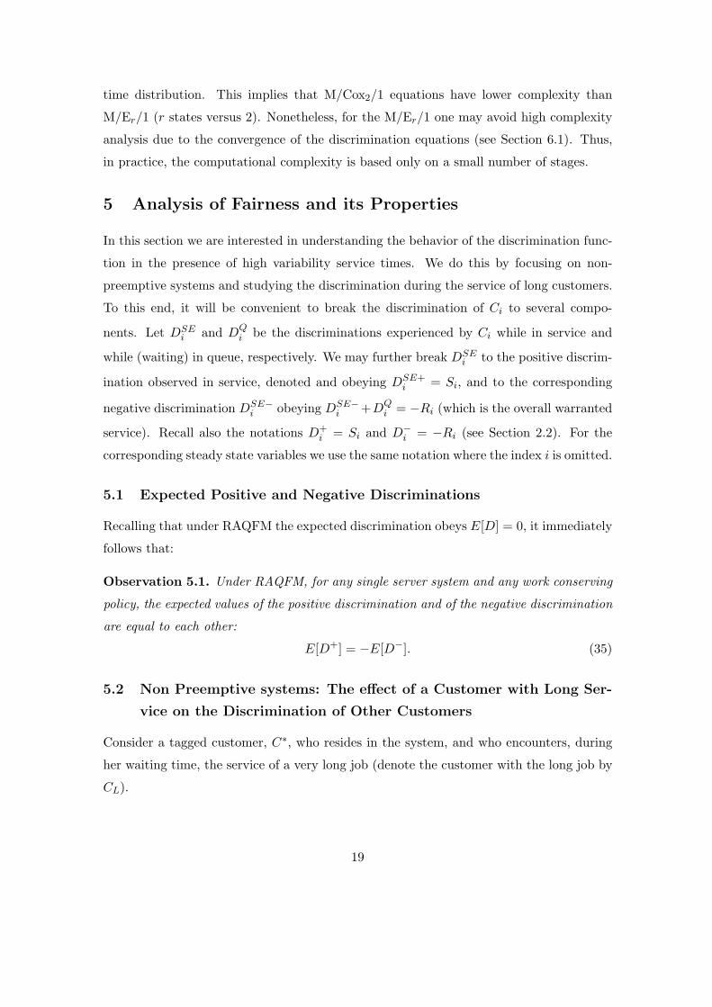
Figure 2: Unfairness for medium variability system, M/E1/1 (Coefficient of variation

γS = 1)

0.1 0.2 0.3 0.4 0.5 0.6 0.7 0.8 0.90

0.5

1

1.5

2

2.5

3

3.5

4

4.5

M/E10

/1 system, γs2=1/10

ρ

Var

[D]

LCFS−PRLCFS−NPRROS−PRROS−NPRFCFS

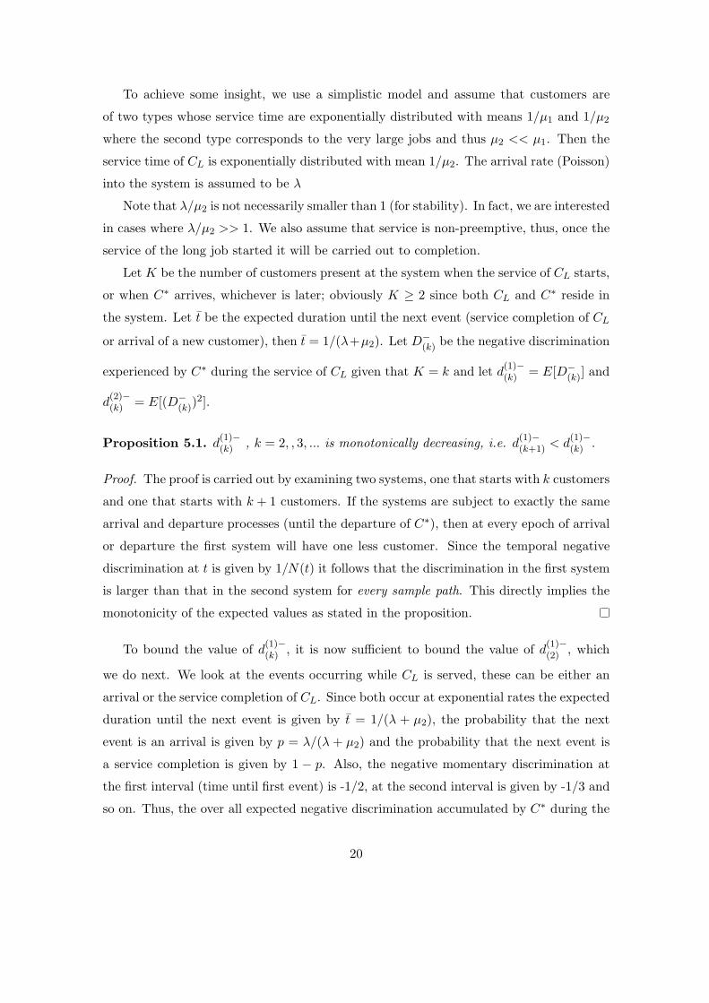
Figure 3: Unfairness for low variability system, M/E10/1 (Coefficient of variation γS =

1/√

10)

In all cases examined we set the mean service time to E[S] = 1 and use the arrival rate

λ to control the system load. We also vary the service time coefficient of variation γS . The

examination is carried out for loads ranging between 0.1 and 0.9 and γS varies through

the values 1/(√

20), 1/(√

15), 1/(√

10), 1/(√

5), 1, 5, 10, 15, 20. For compactness we do not

present here all the results.

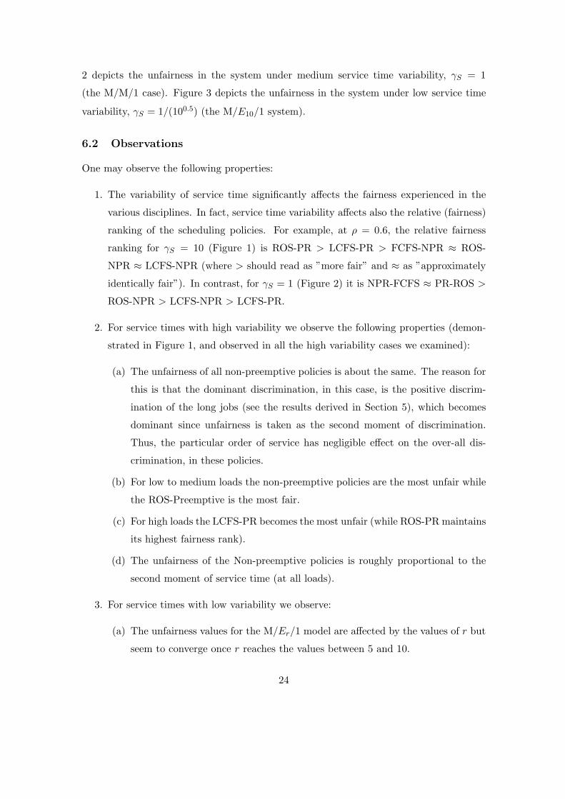
Figure 1 depicts the unfairness in the system under high service time variability γS =

10. The behavior for γS = 5, 15, 20 is quite similar and thus is not presented. Figure

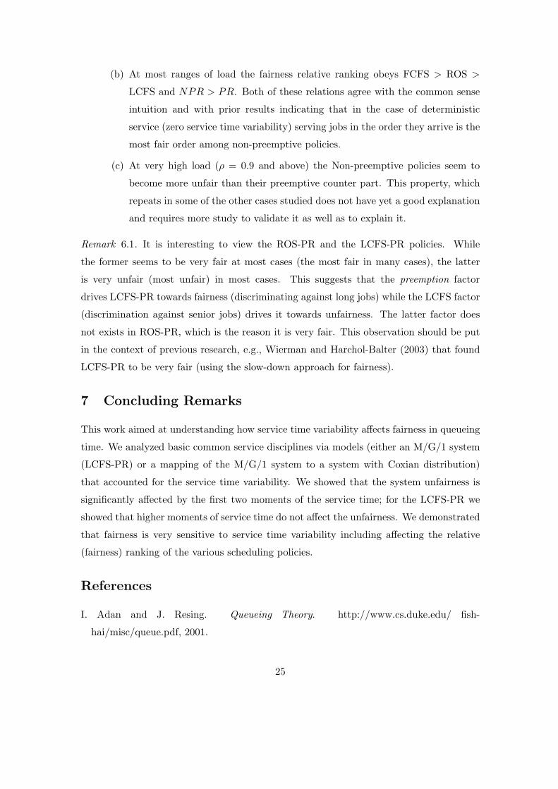
23

2 depicts the unfairness in the system under medium service time variability, γS = 1

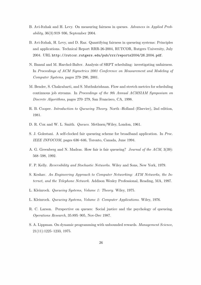
(the M/M/1 case). Figure 3 depicts the unfairness in the system under low service time

variability, γS = 1/(100.5) (the M/E10/1 system).

6.2 Observations

One may observe the following properties:

1. The variability of service time significantly affects the fairness experienced in the

various disciplines. In fact, service time variability affects also the relative (fairness)

ranking of the scheduling policies. For example, at ρ = 0.6, the relative fairness

ranking for γS = 10 (Figure 1) is ROS-PR > LCFS-PR > FCFS-NPR ≈ ROS-

NPR ≈ LCFS-NPR (where > should read as ”more fair” and ≈ as ”approximately

identically fair”). In contrast, for γS = 1 (Figure 2) it is NPR-FCFS ≈ PR-ROS >

ROS-NPR > LCFS-NPR > LCFS-PR.

2. For service times with high variability we observe the following properties (demon-

strated in Figure 1, and observed in all the high variability cases we examined):

(a) The unfairness of all non-preemptive policies is about the same. The reason for

this is that the dominant discrimination, in this case, is the positive discrim-

ination of the long jobs (see the results derived in Section 5), which becomes

dominant since unfairness is taken as the second moment of discrimination.

Thus, the particular order of service has negligible effect on the over-all dis-

crimination, in these policies.

(b) For low to medium loads the non-preemptive policies are the most unfair while

the ROS-Preemptive is the most fair.

(c) For high loads the LCFS-PR becomes the most unfair (while ROS-PR maintains

its highest fairness rank).

(d) The unfairness of the Non-preemptive policies is roughly proportional to the

second moment of service time (at all loads).

3. For service times with low variability we observe:

(a) The unfairness values for the M/Er/1 model are affected by the values of r but

seem to converge once r reaches the values between 5 and 10.

24

(b) At most ranges of load the fairness relative ranking obeys FCFS > ROS >

LCFS and NPR > PR. Both of these relations agree with the common sense

intuition and with prior results indicating that in the case of deterministic

service (zero service time variability) serving jobs in the order they arrive is the

most fair order among non-preemptive policies.

(c) At very high load (ρ = 0.9 and above) the Non-preemptive policies seem to

become more unfair than their preemptive counter part. This property, which

repeats in some of the other cases studied does not have yet a good explanation

and requires more study to validate it as well as to explain it.

Remark 6.1. It is interesting to view the ROS-PR and the LCFS-PR policies. While

the former seems to be very fair at most cases (the most fair in many cases), the latter

is very unfair (most unfair) in most cases. This suggests that the preemption factor

drives LCFS-PR towards fairness (discriminating against long jobs) while the LCFS factor

(discrimination against senior jobs) drives it towards unfairness. The latter factor does

not exists in ROS-PR, which is the reason it is very fair. This observation should be put

in the context of previous research, e.g., Wierman and Harchol-Balter (2003) that found

LCFS-PR to be very fair (using the slow-down approach for fairness).

7 Concluding Remarks

This work aimed at understanding how service time variability affects fairness in queueing

time. We analyzed basic common service disciplines via models (either an M/G/1 system

(LCFS-PR) or a mapping of the M/G/1 system to a system with Coxian distribution)

that accounted for the service time variability. We showed that the system unfairness is

significantly affected by the first two moments of the service time; for the LCFS-PR we

showed that higher moments of service time do not affect the unfairness. We demonstrated

that fairness is very sensitive to service time variability including affecting the relative

(fairness) ranking of the various scheduling policies.

References

I. Adan and J. Resing. Queueing Theory. http://www.cs.duke.edu/ fish-

hai/misc/queue.pdf, 2001.

25

B. Avi-Itzhak and H. Levy. On measuring fairness in queues. Advances in Applied Prob-

ability, 36(3):919–936, September 2004.

B. Avi-Itzhak, H. Levy, and D. Raz. Quantifying fairness in queueing systems: Principles

and applications. Technical Report RRR-26-2004, RUTCOR, Rutgers University, July

2004. URL http://rutcor.rutgers.edu/pub/rrr/reports2004/26 2004.pdf.

N. Bansal and M. Harchol-Balter. Analysis of SRPT scheduling: investigating unfairness.

In Proceedings of ACM Sigmetrics 2001 Conference on Measurement and Modeling of

Computer Systems, pages 279–290, 2001.

M. Bender, S. Chakrabarti, and S. Muthukrishnan. Flow and stretch metrics for scheduling

continuous job streams. In Proceedings of the 9th Annual ACMSIAM Symposium on

Discrete Algorithms, pages 270–279, San Francisco, CA, 1998.

R. B. Cooper. Introduction to Queueing Theory. North -Holland (Elsevier), 2nd edition,

1981.

D. R. Cox and W. L. Smith. Queues. Methuen/Wiley, London, 1961.

S. J. Golestani. A self-clocked fair queueing scheme for broadband application. In Proc.

IEEE INFOCOM, pages 636–646, Toronto, Canada, June 1994.

A. G. Greenberg and N. Madras. How fair is fair queueing? Journal of the ACM, 3(39):

568–598, 1992.

F. P. Kelly. Reversibility and Stochastic Networks. Wiley and Sons, New York, 1979.

S. Keshav. An Engineering Approach to Computer Networking: ATM Networks, the In-

ternet, and the Telephone Network. Addison Wesley Professional, Reading, MA, 1997.

L. Kleinrock. Queueing Systems, Volume 1: Theory. Wiley, 1975.

L. Kleinrock. Queueing Systems, Volume 2: Computer Applications. Wiley, 1976.

R. C. Larson. Perspective on queues: Social justice and the psychology of queueing.

Operations Research, 35:895–905, Nov-Dec 1987.

S. A. Lippman. On dynamic programming with unbounded rewards. Management Science,

21(11):1225–1233, 1975.

26

I. Mann. Queue culture: The waiting line as a social system. Am. J. Sociol., 75:340–354,

1969.

R.A. Marie. Calculating equilibrium probabilities for λ(n)/ck/1/n queue. In Proceedings

Performance, pages 117–125, Toronto, May 1980.

C. Palm. Methods of judging the annoyance caused by congestion. Tele. (English Ed.), 2:

1–20, 1953.

A. Rafaeli, G. Barron, and K. Haber. The effects of queue structure on attitudes. Journal

of Service Research, 5(2):125–139, 2002.

A. Rafaeli, E. Kedmi, D. Vashdi, and G. Barron. Queues and fairness: A multiple study

investigation. Faculty of Industrial Engineering and Management, Technion. Haifa,

Israel. Under review, 2003. URL http://iew3.technion.ac.il/Home/Users/anatr/

JAP-Fairness-Submission.pdf.

D. Raz, B. Avi-Itzhak, and H. Levy. Classes, priorities and fairness in queueing systems.

Technical Report RRR-21-2004, RUTCOR, Rutgers University, June 2004a. URL http:

//rutcor.rutgers.edu/pub/rrr/reports2004/21 2004.pdf.

D. Raz, H. Levy, and B. Avi-Itzhak. A resource-allocation queueing fairness measure. In

Proceedings of Sigmetrics 2004/Performance 2004 Joint Conference on Measurement

and Modeling of Computer Systems, pages 130–141, New York, NY, June 2004b. Also

appears in Performance Evaluation Review, 32(1):130-141.

M. H. Rothkopf and P. Rech. Perspectives on queues: Combining queues is not always

beneficial. Operations Research, 35:906–909, 1987.

W. Whitt. The amount of overtaking in a network of queues. Networks, 14(3):411–426,

1984.

A. Wierman and M. Harchol-Balter. Classifying scheduling policies with respect to unfair-

ness in an M/GI/1. In Proceedings of ACM Sigmetrics 2003 Conference on Measurement

and Modeling of Computer Systems, pages 238 – 249, San Diego, CA, June 2003.

Y. Zhou and H. Sethu. On the relationship between absolute and relative fairness bounds.

IEEE Communication Letters, 6(1):37–39, January 2002.

27

A Appendix

A.1 Conditional Discrimination in M/Er/1

A.1.1 Non-Preemptive LCFS

Let C denote the tagged customer. For consistency we assume that the queue is ordered

in order of arrival and customers are admitted into service from the tail of the queue.

At every slot let a denote the number of customers arrived earlier than C and thus to

be served after C. Let b denote the number of customers arrived later than C and thus

to be served before C. The state Sa,b,j (where j is the stage of the customer in service)

captures all that is needed for predicting the future of C. Note that using this description

a customer is served in Sa,0,j , i.e., when b = 0.

An arriving customer starts either in state S0,0,1 when the system is empty, or in state

Sk−1,1,j when the system is serving a customer at stage j. Thus

E[D|k, j] =

{E[d(k − 1, 1, j)] k > 0E[d(0, 0, 0)] k = j

(44)

E[D2|k, j] =

{E[d(2)(k − 1, 1, j)] k > 0E[d(2)(0, 0, 1)] k = j

(45)

Using the same notations as in Section ?? we have:

c(a, b) =

{− 1

a+b+1 b > 01− 1

a+1 b = 0(46)

Here too, when C is in state Sa,b,j it will encounter one of two possible events:

1. A customer arrives into the system. The probability of this event is λ. If C was in

service (b = 0) it will move to Sa+1,0,j , otherwise to Sa,b+1,j

2. A customer completes its current stage. The probability of this event is µ. If C was

in service and j = r it leaves the system. If C wasn’t in service it moves to Sa,b,j+1

if j 6= r or to Sa,b−1,1 if j = r.

This leads to the following recursive expressions for D(a, b, j). For b > 0

D(a, b, j) =

Tc(a, b) + D(a, b + 1, j) w.p λ

T c(a, b) + D(a, b, j + 1) w.p µ, j 6= r,

T c(a, b) + D(a, b− 1, 1) w.p µ, j = r.

(47)

28

and for b = 0

D(a, 0, j) =

Tc(a, 0) + D(a + 1, 0, j) w.p λ

T c(a, 0) + D(a, 0, j + 1) w.p µ, j 6= r,

T c(a, 0) w.p µ, j = r.

(48)

From these, as in Section 4.2.1, we derive the recursive equations for expressing

d(a, b, j) and d(2)(a, b, j).

For b > 0

d(a, b, j) =

{t(1)c(a, b) + λd(a, b + 1, j) + µd(a, b, j + 1) j 6= r

t(1)c(a, b) + λd(a, b + 1, j) + µd(a, b− 1, 1) j = r(49)

d(2)(a, b, j) = t(2)(c(a, b))2 + λd(2)(a, b + 1, j)

+ 2t(1)c(a, b)λd(a, b + 1, j))+

{µd(2)(a, b, j + 1) + 2t(1)c(a, b)µd(a, b, j + 1) j 6= r

µd(2)(a, b− 1, j) + 2t(1)c(a, b)µd(a, b− 1, 1) j = r(50)

and for b = 0

d(a, 0, j) =

{t(1)c(a, 0) + λd(a + 1, 0, j) + µd(a, 0, j + 1) j 6= r

t(1)c(a, 0) + λd(a + 1, 0, j) j = r(51)

d(2)(a, 0, j) = t(2)(c(a, 0))2 + λd(2)(a + 1, 0, j)+

2t(1)c(a, 0)λd(a + 1, 0, j))+

{µd(2)(a, 0, j + 1) + 2t(1)c(a, 0)µd(a, 0, j + 1) j 6= r

0 j = r(52)

A.1.2 Non-Preemptive ROS

For a tagged customer C, let a denote the number of customers in the system other than

C. Consider a boolean variable s which is 1 if C is in service and 0 if it is waiting. The

29

notation used in this section remains unchanged, except that b is replaced by s. In state

Sa, s, j there are a customers in addition to C, the one in service is in its j-th stage, and

it is C if s = 1 and not C if s = 0.

The momentary discrimination at this state is c(a, s),

c(a, s) =

{− 1

a+1 s = 01− 1

a+1 s = 1(53)

A customer arrives to the system either at state S0,1,1 when it is empty, or at state

Sk,0,j when it serving customer at stage j. Then

E[D|k, j] =

{E[d(k, 0, j)] k > 0E[d(0, 1, 1)] k = 0

(54)

E[D2|k, j] =

{E[d(2)(k, 0, j)] k > 0E[d(2)(0, 1, 1)] k = 0

(55)

When C is in state Sa,s,j it will encounter one of the following possible events:

1. If s = 0 the possible events are:

(a) A customer arrives into the system. The probability of this event is λ and C

will move to Sa+1,0,j .

(b) A customer completes its current stage j, where j 6= r. The probability of this

event is µ and C moves to S(a, 0, j + 1).

(c) A customer completes service, leaves the system and C is chosen to receive

service next. The probability of this event is µ/a. C will move to Sa−1,1,1.

(d) A customer completes service, leaves the system and C is not chosen to receive

service next. The probability of this event is µ(a−1)/a. C will move to Sa−1,0,1.

2. If s = 1 the possible events are:

(a) Same as (1a) but C will move to Sa+1,1,j .

(b) Same as (1b) but C will move to Sa,1,j+1.

(c) The customer in service completes its service. The probability of this event is

µ and C leaves the system.

30

Using the same method as in the previous two sections this leads to the following

recursive expressions:

d(a, s, j) = t(1)c(a, s) + λd(a + 1, s, j)+

µd(a, s, j + 1) j 6= rµad(a− 1, 1, 1) + µa−1

a d(a− 1, 0, 1) j = r, s = 00 j = r, s = 1

(56)

d(2)(a, s, j) = t(2)(c(a, s))2 + λd(2)(a + 1, s, j)+

2t(1)c(a, s)λd(a + 1, s, j)+

µd(2)(a, s, j + 1) + 2t(1)c(a, b)µd(a, s, j + 1)) j 6= rµad(2)(a− 1, 1, 1) + µa−1

a d(2)(a− 1, 0, 1)+2t(1)c(a, s)( µ

ad(a− 1, 1, 1) + µa−1a d(a− 1, 0, 1)) j = r, s = 0

0 j = r, s = 1

(57)

B Conditional Discrimination in M/Cox2/1

Consider the M/Cox2/1 where the service time distribution is a two-stage Coxian. For

this distribution the service is assumed to be composed of two serially arranged stages,

where a new customer that enters service starts with stage 1 and after its completion

enters stage 2 with probability p1. The mean length of stage i is µi, i = 1, 2.

Similarly to M/Er/1 the time between the arrival of a customer and its departure is

slotted by arrivals and stage completions, however, for Coxian service the slot duration

is dependant upon the stage of service in which the served customer is currently found.

Let Ti,j , j = 1, 2, i = 1, 2, . . . be the duration of the i-th slot, where j is the stage of the

served customer. Then, Ti,j is a random variable exponentially distributed with parameter

λ + µj ; the first two moments of Ti,j are t(1)j = 1

λ+µjand t

(2)j = 2

(λ+µj)2= 2(t(1)

j )2. The

probabilities that a slot ends with an arrival or with a stage completion are denoted by λj

and µj respectively.

λj =λ

λ + µjµj =

µj

λ + µj(58)

31

. Similarly to Eq.(22) the system unfairness is expressed as:

E[D2] = P0E[D2|0, 1] +∞∑

k=1

2∑

j=1

Pk,jE[D2|k, j], (59)

B.0.3 FCFS

We preserve the notations of Section 4.2.1 and denote by Sa,b,j the state of a tagged

customer C, where a is the number of customers ahead of C, b is the number of customers

behind C, and j is the stage of customer in service.

The momentary discrimination at state Sa,b,j is given by

c(a, b) =

{− 1

a+b+1 b > 01− 1

b+1 b = 0(60)

Similarly to (24)

E[D|k, j] = E[d(k, 0, j)] (61)

E[D2|k, j] = E[d(2)(k, 0, j)] (62)

Using a similar method of analysis as in Section ?? we have that

d(a, b, j) = t(1)j c(a, b) + λjd(a, b + 1, j)+

{p1µjd(a, b, j + 1) + ∆(a > 0)(1− p1)µjd(a− 1, b, 1) j = 1∆(a > 0)µjd(a− 1, b, 1) j = 2

(63)

where Tj is the duration of the current slot and the served customer is located at stage j

during this slot. The second moment is given by

d(2)(a, b, j) = t(2)j (c(a, b))2 + λd(2)(a, b + 1, j)+

2t(1)j c(a, b)λd(a, b + 1, j)+

p1µjd(2)(a, b, j + 1) + ∆(a > 0)(1− p1)µjd

(2)(a− 1, b, 1)+2t

(1)j c(a, b)(p1µjd

(2)(a, b, j + 1) + ∆(a > 0)(1− p1)µjd(2)(a− 1, b, 1)) j = 1

∆(a > 0)(µjd(2)(a− 1, b, j) + 2t

(1)j c(a, b)µjd(a− 1, b, j))) j = 2

(64)

32

B.0.4 Non-Preemptive LCFS

We preserve the notations of Section A.1.1 and denote by Sa,b,j the state of C, where a

is the number of customers arrived earlier than C and thus to be served after C, b is the

number of customers arrived later than C and thus to be served before C, and j is the

stage of the served customer. The conditional discrimination (Eq.(44), Eq.(45)) and the

momentary discrimination (Eq.(46)) remains the same as in Section A.1.1.

By examining the possible events that C encounter we get that for b > 0

d(a, b, j) = tjc(a, b) + λjd(a, b + 1, j)+

{p1µjd(a, b, j + 1) + (1− p1)µjd(a, b− 1, 1) j = 1µjd(a, b− 1, 1) j = 2

(65)

d(2)(a, b, j) = t(2)j (c(a, b))2 + λjd

(2)(a, b + 1, j) + 2t(1)j c(a, b)d(a, b + 1, j)

p1µjd(2)(a, b, j + 1) + (1− p1)µjd

(2)(a, b− 1, 1)+2t

(1)j c(a, b)(p1µjd(a, b, j + 1) + (1− p1)µjd(a, b− 1, 1)) j = 1

µjd(2)(a, b− 1, 1) + 2t(1)

j c(a, b)µjd(a, b− 1, 1) j = 2

(66)

For b = 0

d(a, 0, j) = tjc(a, 0) + λjd(a + 1, 0, j)+

{p1µjd(a, 0, j + 1) j = 10 j = 2

(67)

d(2)(a, 0, j) = t(2)j (c(a, 0))2 + λjd

(2)(a + 1, 0, j) + 2t(1)j c(a, 0)d(a + 1, 0, j)

{p1µjd

(2)(a, 0, j + 1) + 2t(1)j c(a, 0)p1µjd(a, 0, j + 1) j = 1

0 j = 2(68)

B.0.5 Non Preemptive ROS

We preserve the notations of Section A.1.2 and denote by Sa, s, j the state of C, where

a is the number of customers in the system other than C, s is 1 if C is in service and 0

33

if it is waiting, and j is the state of the served customer. The conditional discrimination

(Eq.(54), Eq.(54)) and the momentary discrimination (Eq.(53)) remains the same as in

Section A.1.2.

By examining the possible events that C encounter we get that

d(a, s, j) = t(1)j c(a, s) + λjd(a + 1, s, j)+

p1µjd(a, s, j + 1)+∆(a > 0)(1− p1)µj( 1

ad(a− 1, 1, 1) + a−1a d(a− 1, 0, 1)) j = 1

∆(a > 0)µj( 1ad(a− 1, 1, 1) + a−1

a d(a− 1, 0, 1)) j = 2

(69)

d(2)(a, b, j) = t(2)j (c(a, s))2 + λjd

(2)(a + 1, s, j)+

2t(1)j c(a, s)λjd(a + 1, s, j)+

p1µj(d(2)(a, s, j + 1) + 2t(1)j c(a, s)d(a, s, j + 1))+

∆(a > 0)(1− p1)µj( 1ad(2)(a− 1, 1, 1) + a−1

a d(2)(a− 1, 0, 1)+2t

(1)j c(a, s)( 1

ad(a− 1, 1, 1) + a−1a d(a− 1, 0, 1)) j = 1

∆(a > 0)µj( 1ad(2)(a− 1, 1, 1) + a−1

a d(2)(a− 1, 0, 1)+2t

(1)j c(a, s)( 1

ad(2)(a− 1, 1, 1) + a−1a d(2)(a− 1, 0, 1)) j = 2

(70)

34