The Effects of Future Capital Investment and R&D ...fm · The Effects of Future Capital Investment and R&D Expenditures on Firms’ Liquidity ... It is important to understand why

The Effects of Future Capital Investment and

R&D Expenditures on Firms’ Liquidity

Christopher F Bauma,b,1, Mustafa Caglayanc, Oleksandr Talaverad

aDepartment of Economics, Boston College, Chestnut Hill, MA 02467 USAbDIW Berlin, Mohrenstraße 58, 10117 Berlin, Germany

cDepartment of Economics, University of Sheffield, Sheffield S10 2TN, UKdDurham Business School, Durham University, Durham DH1 3LB, UK

Abstract

The paper explores factors that lead to accumulation or decumulation of firms’ cash reserves.In particular, we empirically examine whether additional future fixed capital and R&Dinvestment expenditures induce firms to change their liquidity ratio while considering therole of market imperfections. Implementing a dynamic framework on a panel of US, UKand German firms, we find that firms in all three countries make larger adjustments tocash holdings when they plan additional future R&D rather than fixed capital investmentexpenditures. This behavior is particularly prevalent among financially constrained firms.(JEL Classification Numbers: G31, G32)

Key words: cash holdings, fixed investment, R&D investment, dynamic panel regression

Email addresses: [email protected] (Christopher F Baum), [email protected] (MustafaCaglayan), [email protected] (Oleksandr Talavera)

1Corresponding author. Phone 1-617-552-3673, Fax 1-617-552-2308.

November 15, 2012

The Effects of Future Capital Investment and

R&D Expenditures on Firms’ Liquidity

Abstract

The paper explores factors that lead to accumulation or decumulation of firms’ cash

reserves. In particular, we empirically examine whether additional future fixed capital and

R&D investment expenditures induce firms to change their liquidity ratio while considering

the role of market imperfections. Implementing a dynamic framework on a panel of US,

UK and German firms, we find that firms in all three countries make larger adjustments to

cash holdings when they plan additional future R&D rather than fixed capital investment

expenditures. This behavior is particularly prevalent among financially constrained firms.

2

1. Introduction

It is important to understand why firms hold substantial amounts of cash, which earns

little or no interest, rather than channelling those funds towards capital investment projects

or as dividends to shareholders. In an environment with no market imperfections, firms can

tap into financial markets costlessly and need not hold cash (Keynes (1936)) as cash has a

zero net present investment value (Modigliani & Miller (1958)). However, in the presence of

financial frictions, firms do not undertake all positive net present value projects, but rather

choose to save funds for transactions or precautionary motives. In that sense, firms facing

market imperfections must choose their level of liquidity at each point in time while taking

into account current and future business opportunities.

In this paper we empirically examine the changes in firms’ cash holdings, focusing on

the effects of future investment expenditures on the accumulation or decumulation of firms’

cash reserves. Although we are not the first to investigate how firms’ investment expendi-

tures affect their cash holding behavior, our study differs from the rest of the literature on

several grounds. An inspection of the literature shows that researchers have recognized the

significance of current and future investment plans for liquidity management, yet there seems

to be little consensus on how to capture those effects. For instance, some researchers use

current investment expenditures or reported investment plans, while others use Tobin’s Q to

proxy future investment opportunities of the firm. However, all of these strategies have their

drawbacks, as we later discuss. In this paper, we examine the effect of one-period-ahead

additional investment expenditures on firms’ liquidity management behavior. We reason

that a rational manager who plans to expand her firm’s investment in the next period would

take measures to improve the liquid assets of the company so that the project could be

realized despite the potential effects of external or internal financial constraints. In such

circumstances we should observe that firm’s cash holdings will increase.

Our second objective is to examine which type of future investment, fixed capital versus

3

R&D expenditures, would lead to a higher accumulation of cash buffer stocks. We conjecture

that an increase in future R&D expenditures will require firms to increase their cash holdings

by more than that of fixed capital expenditures. Our reasoning, similar to that of the

earlier literature including Brown & Petersen (2011), Hall & Lerner (2009), Bates et al.

(2009), and Opler & Titman (1994), can be explained as follows. In contrast to fixed capital

investment, R&D investment contributes to the stock of intangible capital and cannot be

used as collateral. Thus, firms undergoing large R&D expenditures do not have the financial

flexibility of firms that mainly invest in physical capital, as the latter firms may pledge their

fixed investment as collateral. As most of a firm’s R&D capital stock is represented by human

capital, it would be much more difficult to temporarily reduce R&D expenditures without

losing much of the specialized human capital to other companies.2 Therefore, companies that

have carried out sizable R&D activities are more likely to face greater obstacles in accessing

external financing in comparison to those firms that have largely invested in pledgeable

physical or financial assets. In the presence of financial frictions, this will require firms to

hoard more cash should they plan to increase their R&D expenditures. Another reason

linking expansion in R&D activities to those firms’ increase in cash holdings is the fact that

R&D expenditures have a lengthy and highly uncertain payback.

Some studies in the literature have considered the impact of R&D and fixed investment

expenditures along with several potential firm-specific variables which may also affect firms’

cash holding behavior. In particular, Bates et al. (2009) examine why cash holdings of

US firms increased. They suggest that the precautionary demand for cash can plausibly

explain the secular increase in cash holdings, and show that firms whose R&D expenditures

increase hold more cash, while cash is generally negatively correlated with fixed capital

2As Hall & Lerner (2009) stress (p. 5), a multi-year purchase of machinery could be rescheduled in theface of financial exigencies, but it would be much more difficult to temporarily reduce R&D expenditures.They indicate that this is perhaps the most important distinguishing characteristic of R&D investment, andleads to firms smoothing R&D spending over time to retain their skilled human capital.

4

investment. An earlier, influential study by Opler et al. (1999) also implies that firms’ cash

holdings increase significantly as their capital expenditures-to-assets ratio as well as their

R&D-to-sales ratio increases. In contrast to these studies’ findings, Brown & Petersen (2011)

investigate the factors that affect firms’ R&D expenditures and show that in order to smooth

their R&D activities, firms build up their cash reserves when cash flow is available while

drawing them down when cash flow is reduced.3 In this context, our study is closer to those

of Bates et al. (2009) and Opler et al. (1999). However, we investigate firms’ cash holding

behavior in a dynamic setting as we evaluate the impact of firms’ future investment activities

on this process, and we deal with issues of endogeneity that are not addressed in those

studies. Hence, our work complements the prior literature, as we show that accumulation

of cash holdings is related to firms’ future investment activities, but is most sensitive to

planned R&D activities. These implications are forthcoming from the analytical findings of

Almeida et al. (2011), who present several propositions for firms’ choice of liquid vs. illiquid

investments, and safe vs. risky assets in the context of future financing constraints.

We should also note that recent research highlights the importance of funds raised from

the equity markets to finance R&D expenditures. Kim & Weisbach (2008) provide evidence

that firms who raise funds through IPOs/SEOs experience an increase in their cash holdings,

which is then drawn down to finance various activities including R&D and fixed investment

expenditures.4 Observing their findings, although one can suggest that funds raised from

public offerings can be stored as cash holdings to finance R&D expenditures rather than fixed

investment, it is well accepted in the literature that financial frictions require managers to

hoard cash due to precautionary motives to continue with investment projects when external

3Brown & Petersen (2011) do not investigate firms’ cash accumulation, but rather consider the role ofchanges in cash holdings required to smooth their R&D expenditures.

4For instance, they show that in the first year after an IPO, R&D expenditures increase by 18.5 cents forevery dollar of funding raised.

5

sources of finance may not be available.5 For instance, Bates et al. (2009) provide evidence

from a panel of US manufacturing firms that although firms’ cash holdings have generally

increased in recent years, this is not due to new equity issuance.6 They show that the

observed increase is a reflection of firm characteristics and that the data are consistent with

the presence of precautionary savings.

To test the hypothesis that future fixed capital and R&D investment expenditures have an

impact on firms’ cash holdings, we use large panels of quoted manufacturing firms obtained

from Global COMPUSTAT for the US, UK and Germany over the 1989–2007 period. Our

consideration of firms’ behavior across these three advanced economies provides broader

evidence than the many studies focused on firms in a single country. Cross-country differences

in tax regimes, investment incentives, and firms’ sources of finance provide an additional

source of variation in firms’ behavior.7

We employ the Dynamic Panel Data System-GMM estimator of Blundell & Bond (1998)

to allow for the possible endogeneity of the explanatory variables. Our approach considers

how changes in future investment expenditures may lead to changes in firms’ liquidity. In

contrast to other studies (e.g., Almeida et al. (2004), Ozkan & Ozkan (2004) and Baum

et al. (2008)) and Bates et al. (2009)) that consider the level of cash holdings, we consider

firms’ cash accumulation and decumulation.8 In estimating our models, we take into account

firm-level fixed effects and time effects as well as other firm-specific factors. As the impact of

additional investment expenditures may differ across categories of firms due to the presence

5See, for instance, the first two ‘untested direct model implications’ in Table 1 of Almeida et al. (2011).6Consideration of new equity issuance in our US sample shows that it represents, for the median firm-

year, 0.41% of total assets and 4.94% of cash stocks. Thus, we may conclude that adjustments of cash stockslargely reflect use of internal funds.

7Baum et al. (2011) find significant differences in the financial constraints faced by firms in differentcountries depending on the financial structure in which they operate.

8Bates et al. (2009) consider models of the level and change in the cash ratio. However, their relianceon OLS in a context with several plausibly endogenous regressors, including capital spending and R&Dexpenditures, may cast doubt on their results.

6

of financial frictions, we consider three sample categorizations based on firms’ size, their

dividend payout ratio and their dividend status.

Our analysis provides evidence that firms increase their cash holdings by a larger amount

when they incur additional future R&D expenditures than in the case of future fixed capital

investment. Scrutinizing the data in more detail, we find that this behavior is particularly

prevalent among the so-called ‘financially constrained’ firms (firms that are small in size,

have a low payout ratio, or pay no dividends) that are heavily involved in R&D activities.

Also, similar to the earlier literature, we show that the cash flow sensitivity of cash is higher

for constrained firms with respect to their unconstrained counterparts. Robustness checks

support our findings.

The rest of the paper is organized as follows. Section 2 briefly reviews the literature.

Section 3 presents the model and describes our data. Section 4 provides the empirical

results and Section 5 concludes.

2. Literature Review

2.1. Determinants of Cash Holdings

Keynes (1936) suggests the transaction costs motive and the precautionary motive are

the two major reasons why firms hold cash buffers.9 To attain a certain level of liquidity,

although a firm manager could raise capital by selling assets or issuing new debt or eq-

uity, there are significant costs associated with any of these strategies.10 Bates et al. (2009)

show that over the years, the transactions-based demand for funds declined as both firms

and financial intermediaries developed more efficient transactions technologies. However,

9Keynes (1936) also considers that firms may accumulate cash for speculative purposes. Bates et al.(2009) discuss two other possible motives, based on taxes and agency costs. The tax motive is due to Foleyet al. (2007) who suggest that tax considerations might provide incentives for multinational companies tohoard large amounts of cash. The agency motive is argued by Jensen (1986) that entrenched managers preferto hoard cash, rather than pay dividends, if the firm has poor investment opportunities.

10For instance, see Miller & Orr (1966) who show that firms hold liquid assets as a result of the presenceof brokerage costs involved in raising funds.

7

the precautionary motive, which emphasizes the costs associated with foregone capital in-

vestment opportunities due to financial constraints—as well as managers’ desire to avoid

financial embarrassment in the case of an unexpected shortfall in cash flow—still plays an

important role. For instance, many firms have imperfect access to external funds and they

cannot borrow sizable sums on short notice, particularly if they experience shortfalls in their

cash flow. Furthermore, as firms with weak track records enter the market and experience

various firm-specific risks over the business cycle, it would be difficult for firms’ managers to

successfully raise capital to satisfy their need for liquidity.11 In such circumstances, even if a

lender is willing to extend external credit, it is likely that the premium will be high. Hence,

we would observe that firms follow a financial hierarchy, or ‘pecking order’, as they first tap

cheaper internal sources of funds followed by more expensive alternatives in financing their

activities (see Myers (1984) and Myers & Majluf (1984)). Hence, it should not be surprising

to see that those firms which are adversely affected by financial frictions make use of a cash

buffer in order to minimize the explicit and implicit costs of liquidity management.

The subsequent empirical literature that builds upon the seminal work of Fazzari et al.

(1988) helps us to appreciate why internal funds for the so-called ‘financially constrained’

firms is an important determinant of capital or R&D investment behavior. The basic premise

in this line of empirical work is to capture the differential impact of cash flow on investment

expenditures of firms that are constrained versus those that are not. In other words, the

focus of attention is placed on the dependence of constrained firms on internally generated

funds. Although there are some challenges with respect to the modeling of the problem,

the methodology that one uses to categorize firms, or the control variables used in the

model, it is widely accepted that financial market frictions adversely affect capital investment

expenditures of the constrained firms in comparison to unconstrained firms.12

11Along these lines see Campbell et al. (2001), Fama & French (2004) and Irvine & Pontiff (2009).12See Kaplan & Zingales (1997), Kaplan & Zingales (2000), Fazzari et al. (2000), and Erickson & Whited

8

Given the developments in the literature on fixed investment behavior of firms and finan-

cial frictions, several researchers implement those methodologies to model firms’ liquidity

behavior. Kim et al. (1998), using a sample of US firms, show that firms facing higher costs

of external financing, having more volatile earnings and exhibiting lower returns on assets

carry larger stocks of liquid assets. In a similar vein Opler et al. (1999) provide evidence

that small firms and firms with strong growth opportunities and riskier cash flows hold larger

amounts of cash.13 Almeida et al. (2004) show that constrained firms have a positive cash

flow sensitivity of cash, while unconstrained firms’ cash balance adjustments are not system-

atically related to cash flows. Sufi (2009), using a panel of US firms, also shows that the

cash flow sensitivity of cash is higher for constrained firms, defined as the lack of access to

a line of bank credit. Khurana et al. (2006), using data from several countries, find that the

sensitivity of cash holdings to cash flows decreases with financial development. In a related

study, Faulkender & Wang (2006) and Pinkowitz & Williamson (2007) present evidence that

the value of cash is higher for constrained firms than for unconstrained firms.14

2.2. Effects of Expected Investment Opportunities on Liquidity

Although researchers seek to show that firms’ cash holdings will be related to their in-

vestment opportunities, there is no consensus on how to capture those effects. Researchers

(e.g., Opler et al. (1999)) often incorporate firms’ current investment expenditures in em-

pirical models to capture the impact of investment opportunities on cash holding behavior.

However, empirical models that use current investment expenditures do not necessarily cap-

(2000) for more along these lines.13Pinkowitz & Williamson (2001) report similar findings for firms in Germany and Japan in addition to

those in the US.14There is also active research that relates the value of cash to corporate governance. For instance Dittmar

& Mahrt-Smith (2007) and Harford et al. (2008) present evidence that cash has lower value for firms withweak shareholder rights, pointing out the presence of agency problems. Ozkan & Ozkan (2004), using apanel of UK firms, show that there is a non-monotonic relationship between managerial ownership and cashholdings.

9

ture the effect of future investment. To our knowledge, only Lamont (2000)) has used firms’

investment plans, which more closely address the notion that capital expenditures are largely

determined for a multiperiod horizon. However, data on investment plans are very limited.

Perhaps the most common approach in the literature is the use of Tobin’s Q as a measure

of future investment opportunities of firms, although Erickson & Whited (2000) raise several

warnings about this strategy. For instance, Riddick & Whited (2009), after correcting for

measurement error associated with Tobin’s Q, estimate negative propensities to save out of

cash flow. Almeida et al. (2004) replace the standard Q measure in their basic regressions

model with the average growth of investment over two periods to capture the impact of

current and future investment opportunities on cash holdings.15 In a similar vein, Baum

et al. (2009) study firms’ leverage decisions by employing not current, but realized future

values of the level of capital investment. We follow a similar approach in this study.

While acknowledging the importance of expected investment opportunities, few researchers

distinguish how different types of investment affect corporate liquidity. As we have discussed

above, fixed capital investment leads to the accumulation of pledgeable assets, whereas in-

vestment in R&D may not. We expect that a firm that increases its non-pledgeable invest-

ment activities would hold more liquid assets than a similar firm whose assets may readily

be pledged as collateral. Notably, Almeida & Campello (2007) claim that accumulation of

pledgeable assets supports more borrowing and hence more capital expenditures.16 Bates

et al. (2009), implementing a model where they consider firm-specific factors including fixed

capital and R&D expenditures, provide evidence that firms that are R&D-intensive hold

greater cash buffers against future shocks to cash flows. Opler et al. (1999) show that cash

holdings increase significantly as firms increase their capital expenditures-to-assets ratio as

15Time zero investment opportunities are measured as (I2 + I1)/(2I0).16Almeida & Campello (2007) define tangibility as a function of receivables, inventories and capital stock.

They also use a proxy to measure how easily lenders can liquidate the firm and another proxy based onproduct type (durable/nondurable) of each firm.

10

well as when the R&D-to-sales ratio increases. More recently, Brown & Petersen (2011)

implement dynamic R&D investment models that provide evidence on the importance of

cash reserves, particularly for young firms. However, in none of these studies do researchers

consider firms’ demand for liquidity that arises from future investment activities.

There is also a sizable body of research that focuses on the importance of firms’ financial

constraints and R&D activities. Bond et al. (2005) suggest that financial constrains affect

UK firms’ decision to engage in R&D activity, but not the level of their R&D expenditures.

In a recent paper, Li (2011) argues that financially constrained R&D–intensive firms are more

likely to terminate R&D projects. Furthermore, R&D activities increase the risk of financially

constrained firms, which exacerbates their financial frictions. Czarnitzki & Hottenrott (2011)

find that the availability of internal funds has a more sizable impact on R&D investment,

relative to capital investment, for German firms, with the effect being particularly strong

for small companies. Using a sample of European firms, Brown et al. (2011) show strong

evidence that the availability of finance matters for R&D even after controlling for the use

of external equity financing and smoothing R&D with cash reserves. Evidence of the effects

of financial constrains on R&D activities is also observed for Dutch (Mohnen et al. (2007))

and Slovenian (Bovha-Padilla et al. (2009)) companies.

In our study, we investigate the impact of two types of firms’ future investment activity

on the accumulation of cash holdings: R&D investment versus investment in physical cap-

ital. As discussed in the introduction, the former may be considered as intangible capital

investment, which has a substantially higher marginal cost of external financing because of

its limited pledgeability. Another reason linking expansion in R&D activities to those firms’

increase in cash holdings is the fact that R&D expenditures have a lengthy and highly un-

certain payback. A firm which is engaged in R&D activity may not realize any benefit in

the near future, and may indeed never receive a meaningful return on that investment. This

increases the uncertainty surrounding the firm’s cash flows and working capital. As Hall

11

(2002) points out, uncertain returns from R&D investment might lead to greater asymmet-

ric information and more serious problems of moral hazard, rendering borrowing a costly

option.17 Therefore, one would expect that firms planning to expand their R&D activities

would increase their liquid assets in comparison to other firms which only plan to increase

their fixed capital.

3. Empirical Implementation

3.1. The Baseline Model

To quantify the motivation for firms’ liquid asset holdings, we use a variant of an empirical

specification which is often employed in the literature. The main difference in our approach

is the introduction of two types of investment, fixed capital and R&D, rather than merely

focusing on the role of fixed capital investment. Second, we investigate the effect of changes

in investment expenditures rather than the level. In doing so we would like to capture the

impact of actual changes in investment patterns on the accumulation or decumulation of

cash holdings. If the firm changes either sort of future investment by a sizable amount, we

expect to find a concomitant change in the firm’s cash holdings.

Our baseline model takes the following form:

∆Cashit = α0 + α1∆Cashi,t−1 + α2CashF lowit + α3∆RDi,t+1 (1)

+ α4∆FixInvi,t+1 + α5∆ShortDebtit + α6∆NWCit

+ µi + τt + εit

where i indexes the firm, t the year, ∆Cash is a ratio of the change in cash and short term

investment to beginning-of-period total assets ((Casht − Casht−1)/TAt−1), and CashF low

is defined as income before extraordinary items plus depreciation, also normalized by to-

tal assets. The key coefficients of interest are α3 and α4, which determine the response

17Also see Brown & Petersen (2011), Bates et al. (2009) and Opler & Titman (1994) along these lines.

12

of liquid assets’ holdings to changes in actual future R&D, ∆RD, and fixed capital invest-

ment, ∆FixInv, respectively.18 Additionally, the decision to hold cash crucially depends

on changes in net working capital (∆NWC) and changes in short term debt (∆ShortDebt),

which could be considered as cash substitutes. These two firm-specific characteristics are also

normalized by beginning-of-period total assets (TAt−1). The firm and year-specific effects

are denoted by µ and τ , respectively. Finally, ε is an idiosyncratic error term.

We allow for dynamics in the adjustment of cash holdings, as the firm’s managers (un-

beknownst to the econometrician) may have a multi-year investment plan in place that may

imply several years’ adjustments to their liquidity ratio. Taking this into account, we believe

it is wise to allow the data to indicate whether dynamics in the changes of the liquidity ratio

should play a role in the model.

3.2. The Augmented Model

While allowing for differences between R&D and fixed investment’s effects on corporate

liquidity, Equation (1) does not allow us to explore variations of the cash–future investment

sensitivity between financially constrained and unconstrained firms. To investigate this issue

as well as the differential impact of cash flow between constrained and unconstrained firms,

we specify an extended model in which cash flow and future fixed capital and R&D investment

expenditures are interacted with a vector of firm categories.

The first categorization is based on firm size, given the widespread use of size as a proxy

for financial constraints in the literature. For each firm, we compute the annual average of

their book value of total assets over the full period for which they are observed. We assign the

top and bottom quartiles to large and small firms, respectively, while the two intermediate

quartiles constitute medium size firms. The second category is based on the level of the

dividend payout ratio. The payout categorization is based on the ratio of common share

18We define ∆RDt+1 = (RDt+1 −RDt)/TAt and ∆FixInvt+1 = (Invt+1 − Invt)/TAt.

13

dividend and stock repurchases to total operating income, using the same three quartile-

based categories. The third categorization is dichotomous, considering whether the dividend

payout ratio is positive or zero. There are disagreements in the empirical literature on the

use of the dividend payout ratio (or the presence or absence of dividends) as a proxy for

financial constraints. This is all the more important in a cross-country setting with different

institutional factors. Thus, for robustness, we use two alternative measures based on the

firm’s dividend policy.

Our augmented model takes the form

∆Cashit = α0 + α1∆Cashi,t−1 + [CashF lowit × TY PEit] η + [∆RDi,t+1 × TY PEit] γ1

+ [∆FixInvi,t+1 × TY PEit] γ2 + α5∆ShortDebtit + α6∆NWCit (2)

+ µi + τt + εit

where TY PEit is a vector of dummies capturing one of the categorizations of firms as more

or less likely to face financial constraints.

To aid in comparing results across categories, we estimate a single model where we

interact the category indicators with cash flow and changes of future investment.19 This

approach allows us to properly conduct a test of coefficients’ stability over these categories

of firms. This strategy also allows firms to transition among categories, year by year, rather

than categorizing them once and for all.

To estimate equations (1) and (2) we must take into account the endogeneity of finan-

cial and investment decisions. In particular, including the lagged dependent variable as an

explanatory variable renders a fixed effects estimator biased and inconsistent (see Nickell

(1981)). To overcome this difficulty previous researchers relied heavily on using various

GMM-family estimators (e.g. IV or 2SLS). However, quite often the choice of instruments

19As a robustness check, Section 4.3.4 presents a set of regressions which we carry out for separate cate-gories. Regression results obtained from this investigation provide further support for our main hypothesis.

14

in those settings requires very careful justification. To address this critique, we employ the

Dynamic Panel Data (DPD) estimator that proposes an appropriate set of instruments by

construction. All our models are estimated with the two-step GMM-System estimator, which

combines equations in differences of the variables with equations in levels of the variables.

Individual firm fixed effects are removed by using a first difference transformation.

The reliability of our econometric methodology depends crucially on the validity of the

instruments, which can be evaluated with the Sargan–Hansen J test of overidentifying re-

strictions, asymptotically distributed as χ2 in the number of restrictions. A rejection of the

null hypothesis that instruments are orthogonal to the error process would indicate that the

estimates are not consistent. We also present test statistics for second-order serial correlation

in the error process. In a dynamic panel data context, we expect first order serial correlation,

but should not be able to detect second-order serial correlation if the instruments are appro-

priately uncorrelated with the errors. Our instrument sets have been chosen to ensure that

the orthogonality conditions are satisfied, and that we have avoided the issue of ‘too many

instruments’ discussed in Roodman (2009b). In particular, it is well known that p-values of

1.00 for Hansen J tests indicate that the test of overidentifying restrictions lacks sufficient

power to reject its null in the presence of too many instruments. The GMM-System approach

creates a plethora of instruments, as separate instruments are constructed for the difference

and level equations. We report the number of instruments used in each specification, which

should be well below the number of observations entering the regression. In all cases, the

number of instruments is no greater than 18% of the number of firm-years, and on average

is between 8–11% of the number of firm-years.

As Roodman (2009a) suggests, it is usually necessary to limit the lags of endogenous

variables used as ‘GMM-style’ instruments. We have done so, with lag lengths between 2 and

4 periods applied to the endogenous variables. To ensure validity, we have not included the

first or second lags of changes in actual future R&D, ∆RD, and fixed investment, ∆FixInv.

15

For those variables, lag lengths between 3 and 5 periods have been chosen. The instrument

lag structure for each model has been chosen to ensure that the p-value of the Hansen J

statistic is below unity wherever possible. In each of the models presented below, the Hansen

J statistic for overidentifying restrictions and the Arellano–Bond AR(2) tests show that our

instruments are appropriate and no second order serial correlation is detected, respectively.

3.3. Data

In our empirical investigation we use manufacturing firm-level data extracted from S&P’s

Global COMPUSTAT database which reports accounting information on large corporations.

Although this dataset covers a number of countries, we constrain our investigation to three

advanced economies: the US, UK and Germany. These three advanced economies each have

significant manufacturing sectors—particularly Germany, the world’s leading exporter—but

emphasize different industrial sectors in terms of both capital investment and R&D expen-

ditures.20 These countries allow us to have a reasonably large sample which is essential to

satisfy the asymptotic properties of the GMM-System estimator.

In total, our sample consists of an unbalanced panel of about 32,000 manufacturing firm-

year observations over the period from 1989–2007.21 Prior to estimating our models we apply

a number of sample selection criteria which roughly follow Almeida et al. (2004). First, we

retain companies which have not undergone substantial changes in their composition during

the sample period (e.g., participation in a merger, acquisition or substantial divestment). As

these phenomena are not observable in the data, we calculate the growth rate of each firm’s

total assets and sales, and trim the annual distribution of these growth rates exceeding

20Data availability limits the possibility to consider other leading economies: for instance, although thedataset provides information on a large sample of Japanese firms, data on fixed capital investment are notavailable.

21A firm is considered in the manufacturing sector if its two-digit US Standard Industrial Classification(SIC) code is in the 20–39 range. The database provides this code for non-US firms as well.

16

100%.22 Second, we remove all firms that have fewer than three observations over the

time span. Third, the top and bottom 1% observations of all firm-specific variables are

winsorized. Missing values of R&D expenditures are replaced with zeros. Finally, we drop

all those companies that have cash flow-to-assets ratio lower than −0.5 (−50%) for at least

three years to remove those companies in financial distress.23 The screened US sample is

the largest and consists of 17,813 observations pertaining to 2,006 companies. The German

and UK screened samples consist of 2,306 (352 firms) and 3,202 (505 firms) firm-years’ data,

respectively. All data items are transferred into US dollars and CPI adjusted.

Descriptive statistics for the firm-year observations entering the analysis are presented in

Table 1. As anticipated, there are considerable variations in liquidity ratios across countries.

The highest average liquidity ratio (14.4%) is maintained by US companies, while the lowest

(8.6%) is found for companies headquartered in Germany. Importantly, Table 1 shows that

those US companies that are involved in R&D invest almost as much in R&D as in fixed

capital, while UK firms have a smaller R&D to asset ratio and German firms have the

smallest. We should also note that German firms maintain the highest fixed investment

rates and the highest short-term debt among the three countries.

4. Empirical Results

4.1. Contrast with the Model of Almeida et al. (2004)

Our model can be considered an extension of that developed by Almeida et al. (2004) to

estimate the change in cash holdings (∆C) caused by changes in cash flow and Tobin’s Q,

controlling for firm size.24 In their model, investment opportunities are proxied by Tobin’s Q.

Our data do not include firms’ market value, so we cannot directly estimate their model. We

22We experimented with a more restrictive definition and received quantitatively similar results.23In total, 104 firms have been removed.24We are grateful to an anonymous reviewer for suggesting this discussion be added to the manuscript.

17

proxy Tobin’s Q with the ratio of realized future investment to current investment, defined

in their footnote 20 as (I1 + I2)/(2 × I0).

To illustrate how our modeling strategy differs from that of Almeida et al. (2004), we

present fixed effects results using US, German and UK firms’ data in Table 2, which shows

results from estimating their Equation (8), page 1787, augmented with actual future R&D,

∆NWC, ∆ShortDebt, ∆RD, and ∆FixInv. For comparability, we ignore issues of potential

endogeneity and employ OLS with firm-level fixed effects. Column (1) presents results for

US companies. The common coefficients are quantitatively similar to Almeida et al. (2004)’s

results. Our US estimates also contain positive and significant coefficients for the coeffi-

cients on ∆RD and ∆FixInv. However for the UK and German firms (Columns 2 and 3,

respectively), the Almeida–style results contain insignificant coefficients on the planned R&D

variable. We believe this reflects the serious econometric issues raised by the application of

an OLS fixed effects approach. The proxy for Tobin’s Q introduces obvious measurement

error problems, and ignoring the possible endogeneity in other regressors casts doubt on

the validity of these estimates. For that reason, we do not carry out additional exercises

with this model, which in any case is not in line with the focus of our study. We believe

that adjustment of the firm’s cash buffer stock should be treated as an explicitly dynamic

process. The sizable and significant coefficients on the lagged dependent variables in our

chosen specifications support that interpretation, rendering a fixed effects model biased (per

Nickell (1981)) and inconsistent.

4.2. The Baseline Model

We continue our investigation by implementing a dynamic model (Equation 1) for each

country to explore the effects of cash flow, lagged change in cash holding, change in future

R&D and fixed capital investment expenditures, and changes in non-cash net working capital

and short-term debt ratios on firms’ cash holding behavior. Our premise is that cash flow

and future R&D and fixed investment expenditures should have positive and significant

18

coefficients, with the impact of increases in R&D expenditures greater than that of increases

in fixed capital investment expenditures, as explained earlier. The coefficients of changes in

the non-cash net working capital and short-term debt ratios are expected to be negative.

The impact of R&D expenditures are likely to be most significant for the US firms, as the

data show that US firms are more heavily engaged in R&D activities.

It is useful to note that there are many firms in each country’s sample that do not report

positive R&D spending in any year. If we were attempting to model the firm’s decision to

carry out R&D, and if so how much to spend, we would have to take that stylized fact into

account. In our context, as R&D expenditures only appear on the right side of our estimated

equations, the distribution of that variable is not a concern. In fact, we do not consider

the level of expenditures, but only its change, ∆RDi,t+1. In that context, a firm that never

carries out R&D and a firm that always spends the same amount on R&D are observationally

equivalent. To the extent that zero R&D expenditures are commonly observed—e.g., the

median values of R&D spending in Germany and the UK are both zero—our findings of the

importance of future changes in spending as an important determinant of firms’ liquidity

adjustments are all the more meaningful.

Table 3 presents the results for the dynamic model given in Equation (1). The change

in future fixed investment expenditures is positive for all countries but it is only significant

for the US at the five percent level. That is, an increase in fixed investment behavior

does not necessarily lead to a significant change in cash holdings. This evidence could be

explained by the pledgeability of investments in physical capital. Bester (1985) argues that

collateral can be used as a signaling mechanism to distinguish between high-risk and low-risk

borrowers. In contrast, R&D capital has limited collateral value and it is a riskier type of

investment. We expect that those firms that are planning to increase their R&D investment

expenditures are likely to accumulate liquid assets to finance this type of investment. We

find support for this conjecture. Table 3 provides evidence that the effect of the change

19

in future R&D expenditures leads to a positive and significant increase in liquidity (at the

one percent level for the US and Germany and at the five percent level for the UK). This

observation implies that firms increase their current cash holdings in anticipation of next

period’s R&D expenditures. Furthermore, given the results we can say that firms accumulate

more cash for future R&D expenditures than for future fixed investment expenditures, as

captured by the relative magnitudes of their coefficients. The tests of equality of γ∆RD and

γ∆FixInv coefficients yields p-values of less than 0.10, unambiguously rejecting the null of

equal coefficients.

In Table 3 the coefficient on the lagged dependent variable for all countries is significant

and negative, implying that dynamics of the cash adjustment process are important. Inter-

estingly, our coefficient estimates are very similar to those reported on a firm level by Opler

et al. (1999) from their Eqn. 1, a pure autoregressive model of the change in the cash/assets

ratio. They find a median coefficient of −0.242 at the firm level.25 The table also shows that

an increase in cash flow leads to an accumulation of cash for all countries, as its coefficient is

positive and significant for all three countries at the 1% level. As earlier research has shown,

changes in the non-cash net working capital ratio possess negative and significant coefficients

for all countries. Finally, we find that the change in the short-term debt ratio has a negative

and significant effect on cash accumulation for UK firms, but an insignificant effect in the

US and Germany.

4.3. The Augmented Model

The results given in Tables 4, 5 and 6 present our findings for Equation (2) where we model

firms’ adjustment of their cash balances for different size, dividend and payout categories,

respectively. Each table depicts six models (two per country) where columns 1, 3 and 5 only

25Opler et al. (1999), in their full models, include last period’s deviation from a target cash ratio as anexplanatory factor, using several definitions of the target cash ratio. As we are not testing the ‘static tradeoff’model, we do not include this complication in our dynamic specification.

20

allow the cash flow coefficients to differ across categories. In columns 2, 4 and 6, interactions

with R&D and fixed investment are also included, per Equation (2).

4.3.1. Firms’ Liquidity and the Role of Firm Size

Table 4 presents our results for Equation (2) for different firm size categories. Comparing

results from this table with that of Table 3, we see that the lagged dependent variable and

the changes in non-cash net working capital ratios have similar significance and effects on

firms’ adjustments of their liquidity. Our results show that small firms contribute to their

liquidity more than their larger counterparts do as their cash flow increases. In line with

earlier research, cash flow has a small and insignificant effect on large firms’ liquidity behavior

across all three countries. Although the differences between these effects’ magnitudes across

size categories are generally not statistically significant, the point estimates clearly suggest

the greater importance of cash flow for smaller firms.

Having examined the impact of cash flow across different size categories, we next consider

the effects of R&D and fixed capital expenditure on the liquidity behavior of firms as firm

size is allowed to change for the same set of models. Columns 1, 3, and 5 of the table show

that future capital investment expenditures affect US firms’ liquidity at the one percent level

while the effect is insignificant for the other countries. In contrast, future change in R&D

affects liquidity in all three countries positively and significantly: at the five percent level

for US firms and the ten percent level for UK and German firms.

We next allow the impact of the change in R&D and fixed investment to differ across

different categories along with the effect of cash flow. Inspecting the results given in columns

2, 4 and 6, we see that only US small firms’ liquidity responds to an increase in future capital

investment expenditures. When we consider the effects of future R&D expenditures, we find

that small firms’ future R&D expenditures have a significant and large impact on firms’

liquidity, yet we find no such effect for medium or large firms. This means that medium

and large firms do not significantly increase their liquidity in response to an increase in

21

future R&D expenditures. Financially constrained firms tend to save more in comparison to

unconstrained firms, with future R&D expenditures emerging as an important factor that

induces firms to adjust their cash holdings.

4.3.2. Firms’ Liquidity and the Dividend Payout Ratio

Our second categorization is based on firms’ payout ratios. This categorization allows us

to generate three groups of firms, with low, medium and high dividend payout ratios. We

follow this approach due to the observation that most German and UK firms pay dividends

while some of these may be in fact financially constrained. Hence, inspection of German

and UK firms using this categorization may help us to understand the effects of the changes

in future R&D and fixed investment activities. The disadvantage of this route is that we

will allocate some of the non-dividend paying US firms, which are generally considered by

researchers as financially constrained, to another category. Hence, we would expect that

when evaluating results for US firms that low and medium payout firms in the US would

have similar characteristics.

Table 5 presents our regression results when we investigate firms’ liquidity behavior cate-

gorizing the firms with respect to their dividend payout ratio. In line with our earlier results,

the coefficient of the lagged dependent variable is negative and significant. Also, the signif-

icance and sign of changes in the non-cash net working capital and short-term debt ratios

are unchanged. We also observe that while cash flow for low and medium payout firms has

a positive and significant effect on liquidity the impact of cash flow on those firms that are

in the large payout category, although positive, is insignificant.

When we inspect the impact of a change in future fixed investment on liquidity we find

that the effect is positive for all countries for those countries in the low payout group yet

significant only for the US and the UK. In all cases, changes in future capital investment

does not lead to an increase in firms’ liquidity for medium and high payout firms. When we

examine the impact of a change in future R&D expenditure, we find that low payout firms

22

increase liquidity in all countries. In the US, firms that are in the medium payout category

also increase their liquidity. As discussed earlier, an increase in future R&D investment

induces financially constrained firms to increase their liquidity. While similar behavior is

observed for those firms that increase their fixed capital investment, the evidence is not as

broad as in the case of R&D investment, and the size of the impact on liquidity is always

smaller than that of a change in future R&D investment.

4.3.3. Firms’ Liquidity and Dividend Status

Table 6 presents our regression results when we investigate firms’ liquidity behavior com-

paring dividend-paying with non-dividend-paying firms. In all models, the coefficient of the

lagged dependent variable is negative and significant, indicating that dynamics play an im-

portant role in this relationship. The significance and sign of changes in the non-cash net

working capital and short-term debt ratios are unchanged: non-cash net working capital is

negative and significant for US and UK firms but insignificant for German firms, while the

short-term debt ratio is negative for all cases but significant only for UK firms (see column

5). When we inspect the effect of cash flow for dividend-paying versus non-dividend-paying

firms, we see that non-dividend-paying US firms increase their liquidity significantly in com-

parison to their dividend-paying counterparts. For the case of German and UK firms we find

no difference across dividend paying and non-dividend paying firms, as an increase in their

cash flow leads to an increase in their liquidity.

Next we concentrate on the effects of fixed capital investment and R&D expenditures. In

contrast to the results presented in Table 4, when we categorize the firms between dividend-

paying and non-dividend paying firms, we see no differential effect of future fixed investment

expenditures on either type of firms’ liquidity behavior. However, when we inspect the

impact of an increase in future R&D expenditures, we see that non-dividend-paying firms

augment their liquidity, while dividend-paying firms do not significantly change their liquidity

behavior. This pattern holds for firms in all three economies, supporting the claim that an

23

increase in future R&D expenditures leads to an increase in financially constrained firms’

liquidity.

4.3.4. Robustness checks and a general discussion

The augmented model presented in Tables 4, 5 and 6 constrains some of the coefficients

(e.g., that of the lagged dependent variable, ∆Casht−1) to a single value for different size

classes and dividend categories. This makes it possible to perform formal tests of coefficient

variation across categories in the context of a single equation. Nevertheless, one may suspect

that equations fit separately to each category might exhibit different dynamic behavior.26 To

evaluate the robustness of our findings, we present results obtained from estimating separate

equations for the whole sample and four subsamples (small and large firms, and each dividend

category) of US firms. In doing so, we also include the lagged ratio of new equity issuance to

total assets in the model to investigate whether funds raised from equity issuance will impact

firms’ cash accumulation behavior along the lines suggested by Kim & Weisbach (2008).27,28

The inclusion of this variable allows us to consider whether the coefficients associated with

future fixed investment and R&D expenditures will be qualitatively affected or not.29

These results, for the baseline model, are presented in Table 7.30 Column 1 reports results

for the entire set of US firms, while estimates in columns (2)-(5) are based on subsamples

of small, large, no-dividend-paying and dividend-paying firms, respectively. In general, the

subsample results are qualitatively similar to those presented for the entire set of US firms

26We are grateful to an anonymous reviewer for suggesting that this discussion be added to the manuscript.27The median values of this ratio are 0.004 for the current firm-year, 0.006 averaged over the prior three

firm-years, and 0.008 averaged over the past five firm-years.28Results do not differ when the current ratio of new equity issuance to total assets is used instead of its

lag.29We cannot carry out this exercise for the UK and German subsamples as information on new equity

issuance is only available for US companies.30Estimation of a dynamic panel data model for subsamples is not workable if firms frequently switch

between subsamples. In order to define stable subsamples, we define a dividend-paying firm as a firm thatpaid dividends in 50% or more of observed firm-years, and vice versa.

24

in column (1). We find that the effect of changes in future capital investment is precisely

estimated in the dividend-paying subsample, but not in the other three subsamples. In

these three subsamples, the effects of changes in future R&D expenditures on cash holdings

are precisely estimated. Financially constrained (small or no-dividend-paying) firms have a

greater sensitivity to cash flow and are more likely to adjust their cash stock in anticipation of

changes in future R&D expenditures. For small and non-dividend-paying firms, the effects of

planned R&D and fixed investment are statistically distinguishable at the five per cent level,

and at the six per cent level for all firms. Although, per expectation, new equity issuance

has a uniformly positive effect on firms’ cash accumulation, the impact of the remaining

variables on cash accumulation is not meaningfully altered by its inclusion. The positive

coefficient on new equity issuance suggests that firms use the funds they raise to increase

their cash holdings, quite possibly to finance investment expenditures in subsequent years,

as Kim & Weisbach (2008) suggest.31 However, this effect appears to be weak and we do

not explore this idea further, as it is beyond the objective of this paper.32

A potential issue to be considered in future research is the observational similarity be-

tween the R&D interaction coefficients of small and large US firms, or dividend-paying or

non-paying US firms. For instance in Table 5, although the coefficient of the low payout–

R&D interaction is insignificant and that of the high payout–R&D interaction is significant,

these coefficients cannot be statistically distinguished from each other. This finding for US

firms somewhat weakens the suggestion that financial market frictions affect smaller firms

more severely than larger firms. However, in the UK and German subsamples, the same

set of coefficients are statistically distinguishable, implying the presence of financial market

frictions. The result for US firms could be driven by a number of reasons including the fact

31We thank an anonymous reviewer for suggesting this interpretation.32It may also be the case that the timing of new equity issuance is driven by market timing issues and

underwriters’ recommendations. See Kim & Weisbach (2008) along these lines.

25

that the US firms included in the Global COMPUSTAT database are not really small firms.

Another possibility is that US firms might have greater access to external finance than their

foreign counterparts, regardless of their size, given the greater development of the private

equity and venture capital channels in the US. For future research, it would be useful to

explore this idea using a wider variety set of firms which differ in size and access to financial

markets. For instance, it would be useful to look into public versus non-public firm behavior.

5. Conclusions

In this paper we empirically examine the factors that affect the accumulation or decu-

mulation of cash reserves of firms using data from three advanced economies: the US, UK

and Germany. Our investigation specifically considers the impact of future fixed capital and

R&D expenditures on firms’ liquidity behavior. Although one can expect that an increase in

either type of investment will lead to an improvement in firms’ cash holdings, we conjecture

that the effect of R&D expenditures on firms’ cash holdings should be stronger based on

the observation that R&D investment leads to accumulation of intangible assets and yields

highly uncertain returns. As a result, asymmetric information problems weigh more heavily

in the case of R&D investment in comparison to investment in fixed capital, rendering R&D

activity more dependent on internal financial resources.

To carry out our investigation, we use panels of quoted manufacturing firms obtained from

Global COMPUSTAT for the US, UK and Germany over 1989–2007. The empirical models

implement a dynamic framework to allow the adjustment of cash balances to reflect the many

unobserved factors that may be associated with firms’ multi-year investment plans for both

fixed capital and R&D expenditures. We also consider the impact of market imperfections

resulting in financial constraints by categorizing firms based on size, dividend payout ratio

and dividend status. Our analysis reveals that firms in each country augment their cash

holdings more vigorously in response to additional future R&D expenditures than they do

for increases in future fixed capital investment. Scrutinizing the data in more detail, we

26

find that this behavior is particularly prominent among firms more likely to be financially

constrained: small, low–payout firms or those who do not pay dividends. In line with the

earlier literature, we also show that point estimates of the cash flow sensitivity of cash is

higher for constrained firms with respect to their larger counterparts in all three countries.

The results for US firms are robust to the inclusion of new equity issuance as a source of

cash.

From the policy perspective, one cannot underestimate the importance of technology-

producing mechanisms for knowledge-based economies. Our study reveals that companies

that plan to increase their R&D activities would increase their cash buffers, implying their

need for internally generated funds. This observation holds for all countries in our dataset.

In that sense, our findings are unique in light of previous studies, which have not shown such

diverse and significant effects. In particular we show that future R&D investment has an

economically significant effect on firms’ liquidity behavior, and that this effect is much larger

than that related to future fixed investment. Robustness checks support these findings and

our hypotheses relating to the severity of financial frictions.

Acknowledgements

We acknowledge the constructive suggestions of two anonymous reviewers. We are alsograteful for the comments of participants at the 28th GdRE International Annual Symposiumon Money, Banking and Finance, 2011; the Sixteenth Annual Conference on Panel Data,2010; and seminar participants at Queen’s University Belfast, the University of York, theNational University of Singapore and OFCE/SKEMA Business School, Sophia Antipolis.

27

References

Almeida, H. & Campello, M. (2007), ‘Financial constraints, asset tangibility, and corporateinvestment’, Review of Financial Studies 20(5), 1429–1460.

Almeida, H., Campello, M. & Weisbach, M. (2004), ‘The cash flow sensitivity of cash’,Journal of Finance 59(4), 1777–1804.

Almeida, H., Campello, M. & Weisbach, M. S. (2011), ‘Corporate financial and investmentpolicies when future financing is not frictionless’, Journal of Corporate Finance 17(3), 675–693.

Bates, T. W., Kahle, K. M. & Stulz, R. M. (2009), ‘Why do U.S. firms hold so much morecash than they used to?’, Journal of Finance 64(5), 1985–2021.

Baum, C. F., Caglayan, M., Stephan, A. & Talavera, O. (2008), ‘Uncertainty determinantsof corporate liquidity’, Economic Modelling 25(5), 833–849.

Baum, C. F., Schafer, D. & Talavera, O. (2011), ‘The impact of the financial system’sstructure on firms’ financial constraints’, Journal of International Money and Finance30, 678–691.

Baum, C. F., Stephan, A. & Talavera, O. (2009), ‘The effects of uncertainty on the leverageof nonfinancial firms’, Economic Inquiry 47(2), 216–225.

Bester, H. (1985), ‘Screening vs. rationing in credit markets with imperfect information’,American Economic Review 75(4), 850–55.

Blundell, R. & Bond, S. (1998), ‘Initial conditions and moment restrictions in dynamic paneldata models’, Journal of Econometrics 87, 115–143.

Bond, S., Harhoff, D. & Reenen, J. V. (2005), ‘Investment, R&D and financial constraintsin Britain and Germany’, Annales d’Economie et de Statistique 79-80, 433–460.

Bovha-Padilla, S., Damijan, J. P. & Konings, J. (2009), Financial constraints and the cycli-cality of R&D investment:evidence from Slovenia, LICOS Discussion Papers 23909, LICOS- Centre for Institutions and Economic Performance, K.U.Leuven.

Brown, J. R., Martinsson, G. & Petersen, B. C. (2011), Do financing constraints matter forR&D?, Discussion Paper 1684731, SSRN.

Brown, J. R. & Petersen, B. C. (2011), ‘Cash holdings and R&D smoothing’, Journal ofCorporate Finance 17(3), 694–709.

28

Campbell, J. Y., Lettau, M., Malkiel, B. G. & Xu, Y. (2001), ‘Have individual stocks becomemore volatile? An empirical exploration of idiosyncratic risk’, Journal of Finance 56(1), 1–43.

Czarnitzki, D. & Hottenrott, H. (2011), ‘R&D investment and financing constraints of smalland medium-sized firms’, Small Business Economics 36, 65–83.

Dittmar, A. & Mahrt-Smith, J. (2007), ‘Corporate governance and the value of cash hold-ings’, Journal of Financial Economics 83(3), 599–634.

Erickson, T. & Whited, T. M. (2000), ‘Measurement error and the relationship betweeninvestment and q’, Journal of Political Economy 108(5), 1027–1057.

Fama, E. F. & French, K. R. (2004), ‘New lists: Fundamentals and survival rates’, Journalof Financial Economics 73(2), 229–269.

Faulkender, M. & Wang, R. (2006), ‘Corporate financial policy and the value of cash’, Journalof Finance 61(4), 1957–1990.

Fazzari, S., Hubbard, R. G. & Petersen, B. C. (1988), ‘Financing constraints and corporateinvestment’, Brookings Papers on Economic Activity 19(2), 141–195.

Fazzari, S. M., Hubbard, R. G. & Petersen, B. C. (2000), ‘Investment-cash flow sensitiv-ities are useful: A comment on Kaplan and Zingales’, Quarterly Journal of Economics115(2), 695–705.

Foley, C. F., Hartzell, J. C., Titman, S. & Twite, G. (2007), ‘Why do firms hold so muchcash? A tax-based explanation’, Journal of Financial Economics 86(3), 579–607.

Hall, B. H. (2002), ‘The financing of research and development’, Oxford Review of EconomicPolicy 18(1), 35–51.

Hall, B. H. & Lerner, J. (2009), The financing of R&D and innovation, NBER WorkingPapers 15325, National Bureau of Economic Research, Inc.

Harford, J., Mansi, S. A. & Maxwell, W. F. (2008), ‘Corporate governance and firm cashholdings’, Journal of Financial Economics 87(3), 535–555.

Irvine, P. J. & Pontiff, J. (2009), ‘Idiosyncratic return volatility, cash flows, and productmarket competition’, Review of Financial Studies 22(3), 1149–1177.

Jensen, M. C. (1986), ‘Agency costs of free cash flow, corporate finance, and takeovers’,American Economic Review 76(2), 323–29.

Kaplan, S. N. & Zingales, L. (1997), ‘Do investment-cash flow sensitivities provide usefulmeasures of financing constraints’, Quarterly Journal of Economics 107(1), 196–215.

29

Kaplan, S. N. & Zingales, L. (2000), ‘Investment-cash flow sensitivities are not valid measuresof financing constraints’, Quarterly Journal of Economics 115(2), 707–712.

Keynes, J. M. (1936), The general theory of employment, interest and money, London, Har-court Brace.

Khurana, I. K., Martin, X. & Pereira, R. (2006), ‘Financial development and the cash flowsensitivity of cash’, Journal of Financial and Quantitative Analysis 41(4), 787–808.

Kim, C.-S., Mauer, D. C. & Sherman, A. E. (1998), ‘The determinants of corporate liquidity:Theory and evidence’, Journal of Financial and Quantitative Analysis 33, 335–359.

Kim, W. & Weisbach, M. S. (2008), ‘Motivations for public equity offers: An internationalperspective’, Journal of Financial Economics 87(2), 281–307.

Lamont, O. A. (2000), ‘Investment plans and stock returns’, Journal of Finance 55(6), 2719–2745.

Li, D. (2011), ‘Financial constraints, R&D investment, and stock returns’, Review of Finan-cial Studies 24(9), 2974–3007.

Miller, M. H. & Orr, D. (1966), ‘A model of the demand for money by firms’, QuarterlyJournal of Economics 80(3), 413–435.

Modigliani, F. & Miller, M. (1958), ‘The cost of capital, corporate finance, and the theoryof investment’, American Economic Review 48(3), 261–297.

Mohnen, P., Tiwari, A., Palm, F. & Schim van der Loeff, S. (2007), Financial constraint andR&D investment: Evidence from CIS, UNU-MERIT Working Paper Series 011, UNU-MERIT.

Myers, S. C. (1984), ‘The capital structure puzzle’, Journal of Finance 39(3), 575–92.

Myers, S. C. & Majluf, N. S. (1984), ‘Corporate financing and investment decisions whenfirms have information that investors do not have’, Journal of Financial Economics13, 187–221.

Nickell, S. (1981), ‘Biases in dynamic models with fixed effects’, Econometrica 49, 1417–1426.

Opler, T. C. & Titman, S. (1994), ‘Financial distress and corporate performance’, Journalof Finance 49(3), 1015–40.

Opler, T., Pinkowitz, L., Stulz, R. & Williamson, R. (1999), ‘The determinants and impli-cations of corporate cash holdings’, Journal of Financial Economics 52, 3–46.

30

Ozkan, A. & Ozkan, N. (2004), ‘Corporate cash holdings: An empirical investigation of UKcompanies’, Journal of Banking and Finance 28, 2103–2134.

Pinkowitz, L. & Williamson, R. (2001), ‘Bank power and cash holdings: Evidence fromJapan’, Review of Financial Studies 14(4), 1059–82.

Pinkowitz, L. & Williamson, R. (2007), ‘What is the market value of a dollar of corporatecash?’, Journal of Applied Corporate Finance 19(3), 74–81.

Riddick, L. A. & Whited, T. M. (2009), ‘The corporate propensity to save’, Journal ofFinance 64(4), 1729–1766.

Roodman, D. (2009a), ‘How to do xtabond2: An introduction to difference and system GMMin Stata’, Stata Journal 9(1), 86–136.

Roodman, D. (2009b), ‘A note on the theme of too many instruments’, Oxford Bulletin ofEconomics and Statistics 71(1), 135–158.

Sufi, A. (2009), ‘Bank lines of credit in corporate finance: An empirical analysis’, Review ofFinancial Studies 22(3), 1057–1088.

31

Table 1: Descriptive statistics: All firms, 1989–2007

Panel A: USVariable µ σ Median NCash 0.144 0.176 0.070 17,813Cash Flow 0.067 0.127 0.089 17,813R&D 0.048 0.077 0.019 17,813Fixed Investment 0.052 0.041 0.042 17,813Short Term Debt 0.024 0.054 0.000 17,813

Panel B: GermanyVariable µ σ Median NCash 0.086 0.101 0.049 2,306Cash Flow 0.080 0.096 0.087 2,306R&D 0.013 0.035 0.000 2,306Fixed Investment 0.068 0.049 0.058 2,306Short Term Debt 0.109 0.111 0.068 2,306

Panel C: UKVariable µ σ Median NCash 0.113 0.134 0.071 3,202Cash Flow 0.077 0.119 0.097 3,202R&D 0.020 0.054 0.000 3,202Fixed Investment 0.060 0.044 0.051 3,202Short Term Debt 0.073 0.083 0.045 3,202

Note: All figures are calculated as ratios to the firm’s total assets. µ and σ represent mean and standarddeviation respectively. N is the number of firm-years.

32

Table 2: Fixed effects estimates of ∆Cash

US Germany UK(1) (2) (3)

Cash Flowt 0.286*** 0.126** 0.212***(0.016) (0.054) (0.033)

Sizet 0.015*** 0.024*** 0.020***(0.002) (0.006) (0.006)

Q Proxyt 0.005*** 0.001 0.000(0.001) (0.001) (0.001)

∆NWCt -0.249*** -0.085** -0.394***(0.016) (0.041) (0.044)

∆ShortDebtt+1 -0.292*** -0.066** -0.309***(0.024) (0.033) (0.036)

∆RDt+1 0.288*** -0.066 -0.169(0.048) (0.090) (0.130)

∆Fix. Investmentt+1 0.161*** 0.157*** 0.075(0.034) (0.045) (0.048)

Firm-years 18,440 2,263 3,198Firms 2,013 347 505Test γ∆RD = γ∆FixInv, pvalue 0.030 0.023 0.073

Note: Estimates produced by OLS two-way fixed effects with cluster-robust standard errors, clustering by

firm. * p < 0.10, ** p < 0.05, *** p < 0.01.

33

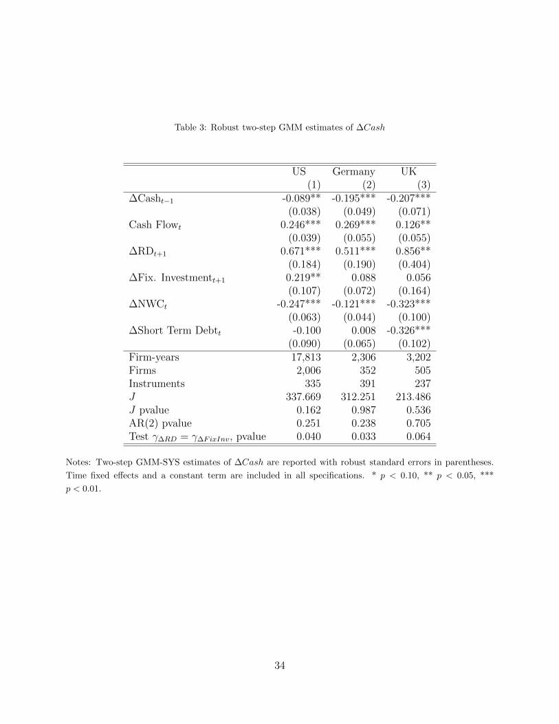
Table 3: Robust two-step GMM estimates of ∆Cash

US Germany UK(1) (2) (3)

∆Casht−1 -0.089** -0.195*** -0.207***(0.038) (0.049) (0.071)

Cash Flowt 0.246*** 0.269*** 0.126**(0.039) (0.055) (0.055)

∆RDt+1 0.671*** 0.511*** 0.856**(0.184) (0.190) (0.404)

∆Fix. Investmentt+1 0.219** 0.088 0.056(0.107) (0.072) (0.164)

∆NWCt -0.247*** -0.121*** -0.323***(0.063) (0.044) (0.100)

∆Short Term Debtt -0.100 0.008 -0.326***(0.090) (0.065) (0.102)

Firm-years 17,813 2,306 3,202Firms 2,006 352 505Instruments 335 391 237J 337.669 312.251 213.486J pvalue 0.162 0.987 0.536AR(2) pvalue 0.251 0.238 0.705Test γ∆RD = γ∆FixInv, pvalue 0.040 0.033 0.064

Notes: Two-step GMM-SYS estimates of ∆Cash are reported with robust standard errors in parentheses.

Time fixed effects and a constant term are included in all specifications. * p < 0.10, ** p < 0.05, ***

p < 0.01.

34

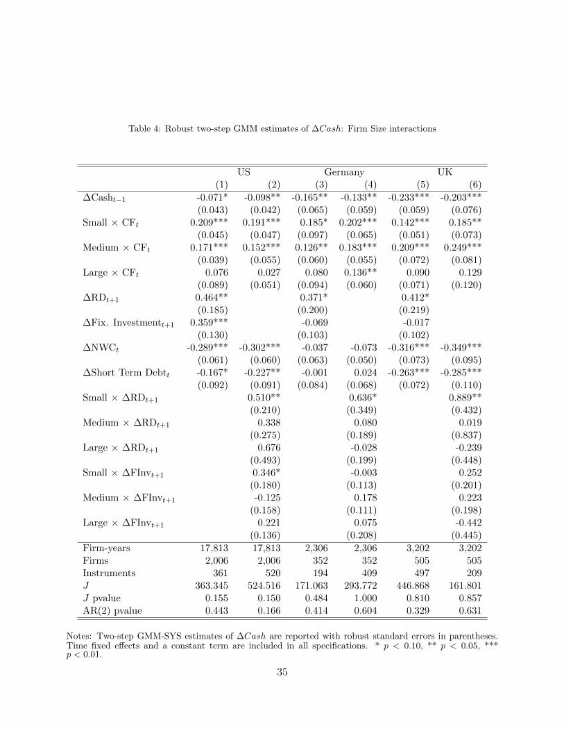
Table 4: Robust two-step GMM estimates of ∆Cash: Firm Size interactions

US Germany UK(1) (2) (3) (4) (5) (6)

∆Casht−1 -0.071* -0.098** -0.165** -0.133** -0.233*** -0.203***(0.043) (0.042) (0.065) (0.059) (0.059) (0.076)

Small × CFt 0.209*** 0.191*** 0.185* 0.202*** 0.142*** 0.185**(0.045) (0.047) (0.097) (0.065) (0.051) (0.073)

Medium × CFt 0.171*** 0.152*** 0.126** 0.183*** 0.209*** 0.249***(0.039) (0.055) (0.060) (0.055) (0.072) (0.081)

Large × CFt 0.076 0.027 0.080 0.136** 0.090 0.129(0.089) (0.051) (0.094) (0.060) (0.071) (0.120)

∆RDt+1 0.464** 0.371* 0.412*(0.185) (0.200) (0.219)

∆Fix. Investmentt+1 0.359*** -0.069 -0.017(0.130) (0.103) (0.102)

∆NWCt -0.289*** -0.302*** -0.037 -0.073 -0.316*** -0.349***(0.061) (0.060) (0.063) (0.050) (0.073) (0.095)

∆Short Term Debtt -0.167* -0.227** -0.001 0.024 -0.263*** -0.285***(0.092) (0.091) (0.084) (0.068) (0.072) (0.110)

Small × ∆RDt+1 0.510** 0.636* 0.889**(0.210) (0.349) (0.432)

Medium × ∆RDt+1 0.338 0.080 0.019(0.275) (0.189) (0.837)

Large × ∆RDt+1 0.676 -0.028 -0.239(0.493) (0.199) (0.448)

Small × ∆FInvt+1 0.346* -0.003 0.252(0.180) (0.113) (0.201)

Medium × ∆FInvt+1 -0.125 0.178 0.223(0.158) (0.111) (0.198)

Large × ∆FInvt+1 0.221 0.075 -0.442(0.136) (0.208) (0.445)

Firm-years 17,813 17,813 2,306 2,306 3,202 3,202Firms 2,006 2,006 352 352 505 505Instruments 361 520 194 409 497 209J 363.345 524.516 171.063 293.772 446.868 161.801J pvalue 0.155 0.150 0.484 1.000 0.810 0.857AR(2) pvalue 0.443 0.166 0.414 0.604 0.329 0.631

Notes: Two-step GMM-SYS estimates of ∆Cash are reported with robust standard errors in parentheses.Time fixed effects and a constant term are included in all specifications. * p < 0.10, ** p < 0.05, ***p < 0.01.

35

Table 5: Robust two-step GMM estimates of ∆Cash: Dividend Payout Ratio interactions

US Germany UK(1) (2) (3) (4) (5) (6)

∆Casht−1 -0.098** -0.102*** -0.225*** -0.222*** -0.269*** -0.203***(0.041) (0.038) (0.055) (0.045) (0.050) (0.041)

Low Payout×CFt 0.164*** 0.206*** 0.377*** 0.276*** 0.133** 0.102*(0.045) (0.037) (0.091) (0.078) (0.063) (0.061)

Medium Payout×CFt 0.203*** 0.017 0.212*** 0.118** 0.267*** 0.256***(0.053) (0.083) (0.073) (0.053) (0.081) (0.072)

High Payout×CFt 0.023 -0.136 0.192** 0.157 0.137 0.164(0.044) (0.084) (0.094) (0.098) (0.089) (0.107)

∆RDt+1 0.503*** 0.374*** 0.493*(0.194) (0.140) (0.268)

∆Fix. Investmentt+1 0.263** 0.007 0.088(0.109) (0.069) (0.109)

∆NWCt -0.249*** -0.271*** -0.086* -0.029 -0.208*** -0.297***(0.055) (0.058) (0.045) (0.041) (0.080) (0.071)

∆Short Term Debtt -0.171* -0.139* -0.003 -0.035 -0.237*** -0.326***(0.094) (0.083) (0.072) (0.055) (0.074) (0.078)

Low Payout×∆RDt+1 0.512*** 0.654* 0.845**(0.190) (0.394) (0.355)

Medium Payout×∆RDt+1 1.383** 0.133 -0.131(0.587) (0.199) (0.407)

High Payout×∆RDt+1 0.776 -0.306 0.629(0.570) (0.791) (0.417)

Low Payout×∆FInvt+1 0.363** 0.185 0.341***(0.167) (0.165) (0.126)

Medium Payout×∆FInvt+1 -0.058 -0.028 -0.010(0.176) (0.091) (0.176)

High Payout×∆FInvt+1 0.069 -0.093 0.212(0.200) (0.137) (0.229)




p < 0.01. 36

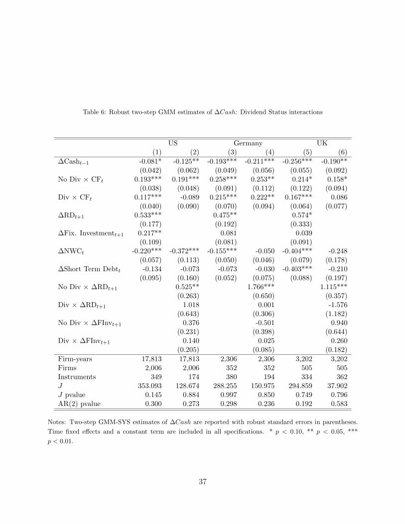
Table 6: Robust two-step GMM estimates of ∆Cash: Dividend Status interactions

US Germany UK(1) (2) (3) (4) (5) (6)

∆Casht−1 -0.081* -0.125** -0.193*** -0.211*** -0.256*** -0.190**(0.042) (0.062) (0.049) (0.056) (0.055) (0.092)

No Div × CFt 0.193*** 0.191*** 0.258*** 0.253** 0.214* 0.158*(0.038) (0.048) (0.091) (0.112) (0.122) (0.094)

Div × CFt 0.117*** -0.089 0.215*** 0.222** 0.167*** 0.086(0.040) (0.090) (0.070) (0.094) (0.064) (0.077)

∆RDt+1 0.533*** 0.475** 0.574*(0.177) (0.192) (0.333)

∆Fix. Investmentt+1 0.217** 0.081 0.039(0.109) (0.081) (0.091)

∆NWCt -0.220*** -0.372*** -0.155*** -0.050 -0.404*** -0.248(0.057) (0.113) (0.050) (0.046) (0.079) (0.178)

∆Short Term Debtt -0.134 -0.073 -0.073 -0.030 -0.403*** -0.210(0.095) (0.160) (0.052) (0.075) (0.088) (0.197)

No Div × ∆RDt+1 0.525** 1.766*** 1.115***(0.263) (0.650) (0.357)

Div × ∆RDt+1 1.018 0.001 -1.576(0.643) (0.306) (1.182)

No Div × ∆FInvt+1 0.376 -0.501 0.940(0.231) (0.398) (0.644)

Div × ∆FInvt+1 0.140 0.025 0.260(0.205) (0.085) (0.182)




p < 0.01.

37

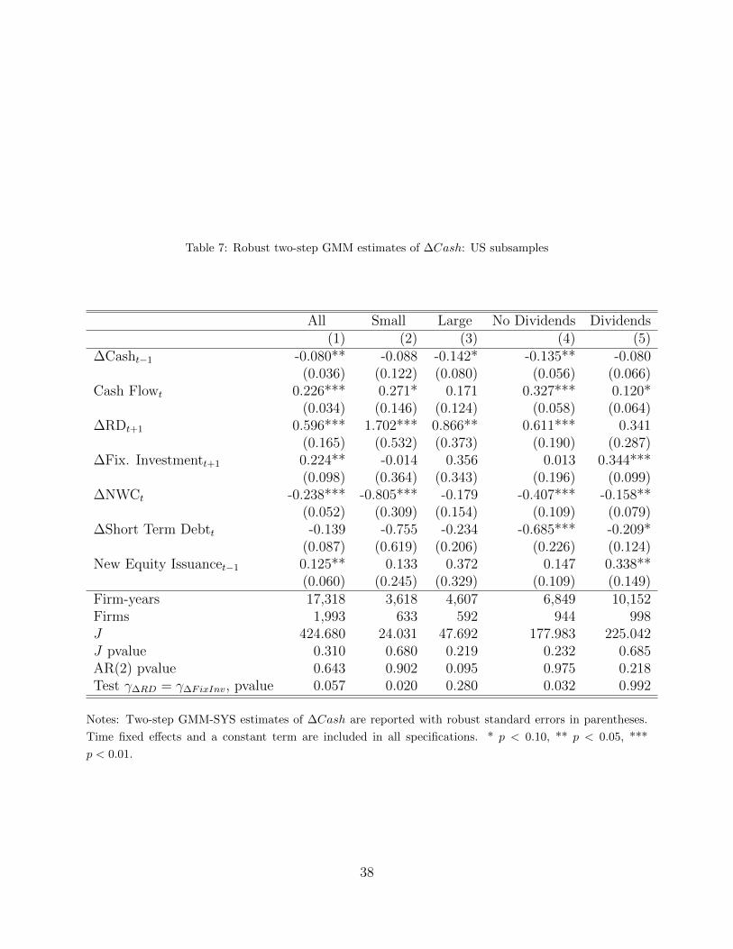
Table 7: Robust two-step GMM estimates of ∆Cash: US subsamples

All Small Large No Dividends Dividends(1) (2) (3) (4) (5)

∆Casht−1 -0.080** -0.088 -0.142* -0.135** -0.080(0.036) (0.122) (0.080) (0.056) (0.066)

Cash Flowt 0.226*** 0.271* 0.171 0.327*** 0.120*(0.034) (0.146) (0.124) (0.058) (0.064)

∆RDt+1 0.596*** 1.702*** 0.866** 0.611*** 0.341(0.165) (0.532) (0.373) (0.190) (0.287)

∆Fix. Investmentt+1 0.224** -0.014 0.356 0.013 0.344***(0.098) (0.364) (0.343) (0.196) (0.099)

∆NWCt -0.238*** -0.805*** -0.179 -0.407*** -0.158**(0.052) (0.309) (0.154) (0.109) (0.079)

∆Short Term Debtt -0.139 -0.755 -0.234 -0.685*** -0.209*(0.087) (0.619) (0.206) (0.226) (0.124)

New Equity Issuancet−1 0.125** 0.133 0.372 0.147 0.338**(0.060) (0.245) (0.329) (0.109) (0.149)

Firm-years 17,318 3,618 4,607 6,849 10,152Firms 1,993 633 592 944 998J 424.680 24.031 47.692 177.983 225.042J pvalue 0.310 0.680 0.219 0.232 0.685AR(2) pvalue 0.643 0.902 0.095 0.975 0.218Test γ∆RD = γ∆FixInv, pvalue 0.057 0.020 0.280 0.032 0.992



p < 0.01.

38

Documents

The Effects of Future Capital Investment and R&D ...fm · The Effects of Future Capital Investment and R&D Expenditures on Firms’ Liquidity ... It is important to understand why