The Effect of Artificial Light on the Community Structure

Louisiana State UniversityLSU Digital Commons

LSU Master's Theses Graduate School

2016

The Effect of Artificial Light on the CommunityStructure and Distribution of Reef-AssociatedFishes at Oil and Gas Platforms in the NorthernGulf of MexicoVictoria Anne BarkerLouisiana State University and Agricultural and Mechanical College

Follow this and additional works at: https://digitalcommons.lsu.edu/gradschool_theses

Part of the Oceanography and Atmospheric Sciences and Meteorology Commons

This Thesis is brought to you for free and open access by the Graduate School at LSU Digital Commons. It has been accepted for inclusion in LSUMaster's Theses by an authorized graduate school editor of LSU Digital Commons. For more information, please contact [email protected].

Recommended CitationBarker, Victoria Anne, "The Effect of Artificial Light on the Community Structure and Distribution of Reef-Associated Fishes at Oiland Gas Platforms in the Northern Gulf of Mexico" (2016). LSU Master's Theses. 3620.https://digitalcommons.lsu.edu/gradschool_theses/3620

https://digitalcommons.lsu.edu?utm_source=digitalcommons.lsu.edu%2Fgradschool_theses%2F3620&utm_medium=PDF&utm_campaign=PDFCoverPages

https://digitalcommons.lsu.edu/gradschool_theses?utm_source=digitalcommons.lsu.edu%2Fgradschool_theses%2F3620&utm_medium=PDF&utm_campaign=PDFCoverPages

https://digitalcommons.lsu.edu/gradschool?utm_source=digitalcommons.lsu.edu%2Fgradschool_theses%2F3620&utm_medium=PDF&utm_campaign=PDFCoverPages

https://digitalcommons.lsu.edu/gradschool_theses?utm_source=digitalcommons.lsu.edu%2Fgradschool_theses%2F3620&utm_medium=PDF&utm_campaign=PDFCoverPages

http://network.bepress.com/hgg/discipline/186?utm_source=digitalcommons.lsu.edu%2Fgradschool_theses%2F3620&utm_medium=PDF&utm_campaign=PDFCoverPages

https://digitalcommons.lsu.edu/gradschool_theses/3620?utm_source=digitalcommons.lsu.edu%2Fgradschool_theses%2F3620&utm_medium=PDF&utm_campaign=PDFCoverPages

mailto:[email protected]

THE EFFECT OF ARTIFICIAL LIGHT ON THE COMMUNITY STRUCTURE AND DISTRIBUTION OF REEF-ASSOCIATED FISHES AT OIL AND GAS PLATFORMS

IN THE NORTHERN GULF OF MEXICO

A Thesis

Submitted to the Graduate Faculty of the Louisiana State University and

Agricultural and Mechanical College in partial fulfillment of the

requirements for the degree of Masters of Science

in

The College of Oceanography and Coastal Sciences

by Victoria A Barker

B.S., University of South Carolina, 2013 May 2016

ii

ACKNOWLEDGEMENTS

First and foremost, I would like to thank my academic advisor, Dr. James H.

Cowan, Jr., for this incredible opportunity to work and study at LSU. During my time

here, I have had access to incredible resources and the ability to share my results not only

at LSU, but also at international conferences. I feel privileged to be selected as a Cowan

lab student and have immensely enjoyed my time conducting offshore research with

some of the kindest and most dedicated people I have ever met. I would like to thank my

committee members, Dr. Kenneth Rose and Dr. Kevin Xu, for their time and support over

the course of my Masters. They served not only as committee members but also as

excellent professors. My sincerest gratitude to Dr. James Geagan, Dr. Brian Marx,

Stephen Potts, and David Reeves, who tirelessly assisted me with my statistics and never-

ending coding projects.

I am eternally grateful for Dave Nieland, the best lab manager/chum

maker/fisherman one could ask for. He was always willing to lend an ear and has done

more for the advancement of my degree than he could possible know. Further, this

project would never have been completed without the unflagging assistance of Captain

Thomas Tunstall and the crew of the Blazing 7. Offshore trips were never dull and I owe

Thomas for wrestling every shark we brought on board!

I was blessed to join a very tight knit lab group and my lab mates were not only

my colleagues but also my closest friends. Thank you to Kristin Foss, my collaborator,

office mate, and fellow Chilean traveler, for your kind words and constant support over

the past three years. You are without a doubt the most prepared and hard working person

I know! Thanks to Lizz Keller, my fellow Wine Walk Wednesday-er, for nights dressed

iii

up at charity banquets and for always throwing a fantastic tailgate. Thank you to Alayna

Petre and Emily Reynolds for teaching me the ins and outs of offshore research and how

to operate all of the software programs. A big thank you to Ashley Baer, Jackie McCool,

Sarah Margolis, Kat Ellis, Mario Souza, and Haixue Shen for your help offshore and in

the lab.

Finally, a huge thank you to my family and friends who supported me throughout

this lengthy endeavor. To Havalend Steinmuller, who was always there at the phone to

keep me sane, I will never be able to thank you enough for being such an incredible

friend during what was at times a challenging process. I know you’re going to do

amazing things with your doctorate! To my family, I owe you the biggest debt of

gratitude of all. You have always supported my dream of obtaining my Masters and have

stuck by me through all that that decision entailed. Thank you for your love, support, and

guidance.

Funding was provided by the Louisiana Department of Fish and Wildlife and

would not have been possible without their assistance. Oil and gas platforms were owned

and operated by Apache Shelf, Inc., Fieldwood Energy LLC, and Arena Offshore, LP.

This project could never have been completed without their support and access.

iv

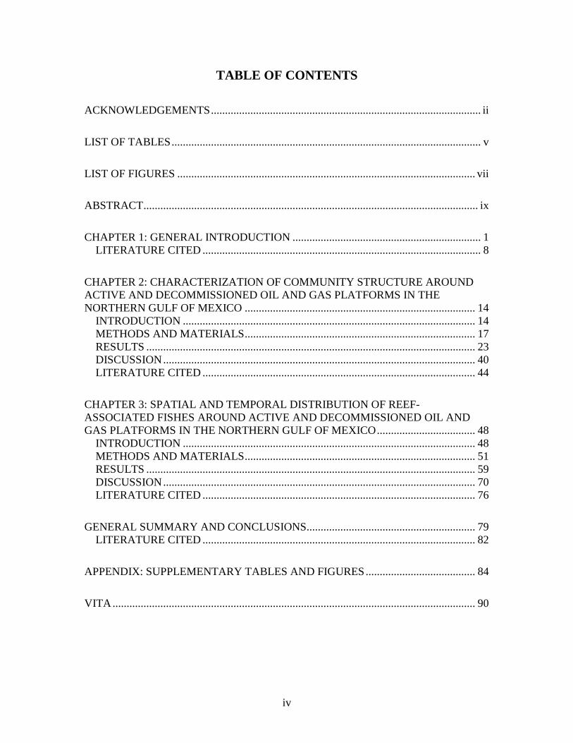
TABLE OF CONTENTS ACKNOWLEDGEMENTS ................................................................................................ ii LIST OF TABLES .............................................................................................................. v LIST OF FIGURES .......................................................................................................... vii ABSTRACT ....................................................................................................................... ix CHAPTER 1: GENERAL INTRODUCTION ................................................................... 1

LITERATURE CITED ................................................................................................... 8 CHAPTER 2: CHARACTERIZATION OF COMMUNITY STRUCTURE AROUND ACTIVE AND DECOMMISSIONED OIL AND GAS PLATFORMS IN THE NORTHERN GULF OF MEXICO .................................................................................. 14

INTRODUCTION ........................................................................................................ 14 METHODS AND MATERIALS .................................................................................. 17 RESULTS ..................................................................................................................... 23 DISCUSSION ............................................................................................................... 40 LITERATURE CITED ................................................................................................. 44

CHAPTER 3: SPATIAL AND TEMPORAL DISTRIBUTION OF REEF-ASSOCIATED FISHES AROUND ACTIVE AND DECOMMISSIONED OIL AND GAS PLATFORMS IN THE NORTHERN GULF OF MEXICO ................................... 48

INTRODUCTION ........................................................................................................ 48 METHODS AND MATERIALS .................................................................................. 51 RESULTS ..................................................................................................................... 59 DISCUSSION ............................................................................................................... 70 LITERATURE CITED ................................................................................................. 76

GENERAL SUMMARY AND CONCLUSIONS............................................................ 79

LITERATURE CITED ................................................................................................. 82 APPENDIX: SUPPLEMENTARY TABLES AND FIGURES ....................................... 84 VITA ................................................................................................................................. 90

v

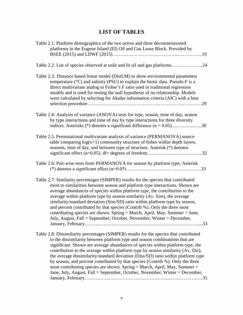
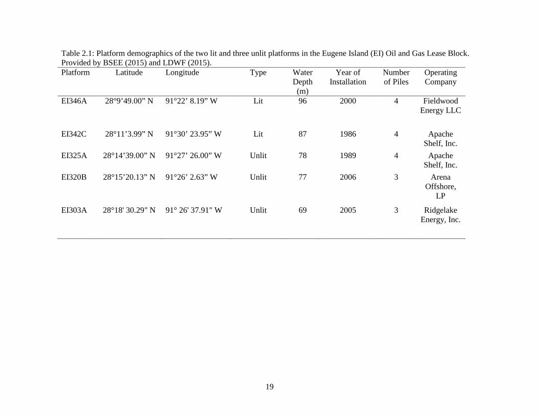
LIST OF TABLES Table 2.1: Platform demographics of the two active and three decommissioned

platforms in the Eugene Island (EI) Oil and Gas Lease Block. Provided by BSEE (2015) and LDWF (2015)…………………………………...……………19

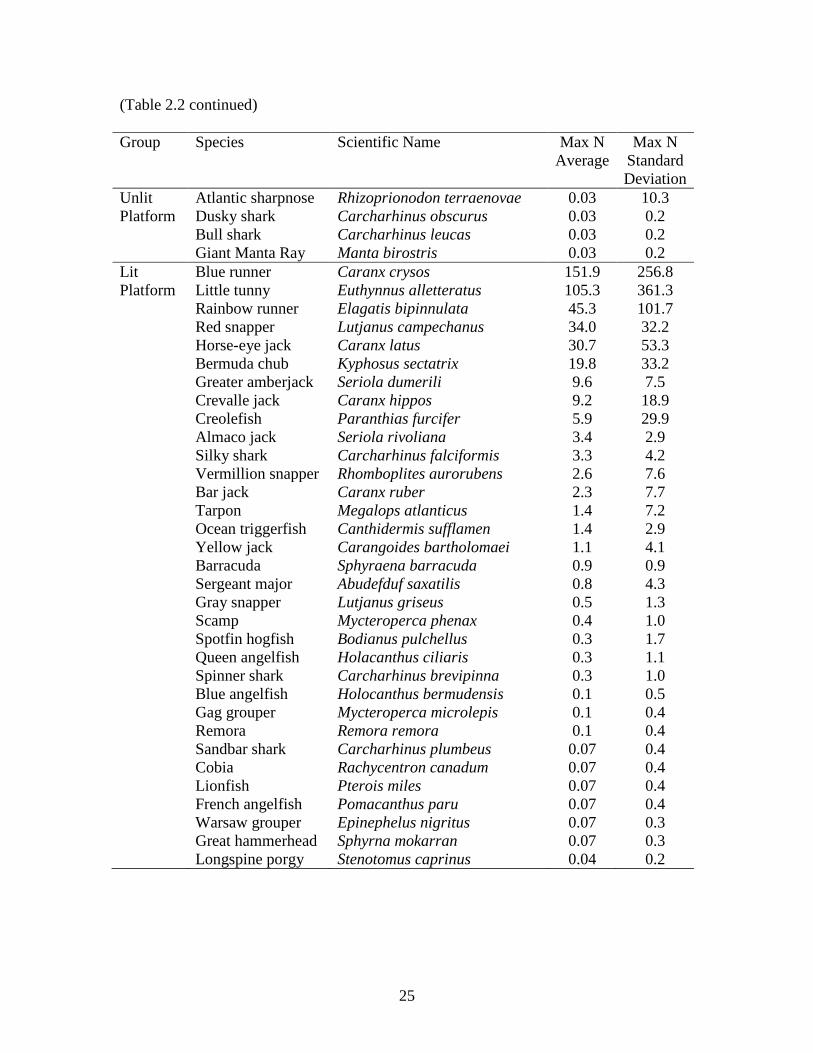
Table 2.2: List of species observed at unlit and lit oil and gas platforms………………..24 Table 2.3: Distance based linear model (DistLM) to show environmental parameters

temperature (°C) and salinity (PSU) to explain the biotic data. Pseudo-F is a direct multivariate analog to Fisher’s F ratio used in traditional regression models and is used for testing the null hypothesis of no relationship. Models were calculated by selecting for Akaike information criteria (AIC) with a best selection procedure………………………………………………………………29

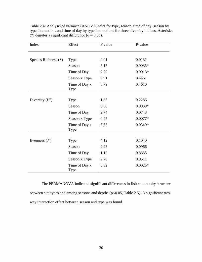
Table 2.4: Analysis of variance (ANOVA) tests for type, season, time of day, season

by type interactions and time of day by type interactions for three diversity indices. Asterisks (*) denotes a significant difference (α = 0.05)…………...…..30

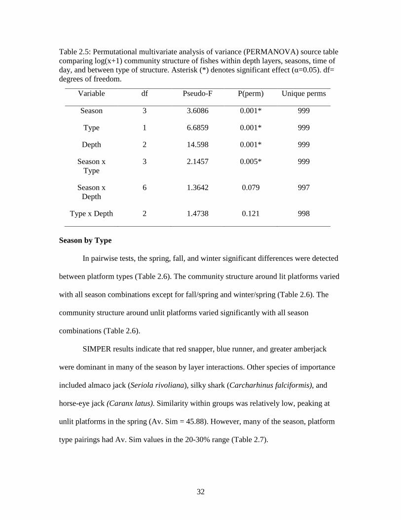
Table 2.5. Permutational multivariate analysis of variance (PERMANOVA) source

table comparing log(x+1) community structure of fishes within depth layers, seasons, time of day, and between type of structure. Asterisk (*) denotes significant effect (α=0.05). df= degrees of freedom……………………………..32

Table 2.6: Pair-wise tests from PERMANOVA for season by platform type; Asterisk (*) denotes a significant effect (α=0.05)………………………. ……………….33

Table 2.7: Similarity percentages (SIMPER) results for the species that contributed

most to similarities between season and platform type interactions. Shown are average abundances of species within platform type, the contribution to the average within platform type by season similarity (Av. Sim), the average similarity/standard deviation (Sim/SD) ratio within platform type by season, and percent contributed by that species (Contrib %). Only the three most contributing species are shown. Spring = March, April, May, Summer = June, July, August, Fall = September, October, November, Winter = December, January, February………………………………………………………………...33

Table 2.8: Dissimilarity percentages (SIMPER) results for the species that contributed to the dissimilarity between platform type and season combinations that are significant. Shown are average abundances of species within platform type, the contribution to the average within platform type by season similarity (Av. Dis), the average dissimilarity/standard deviation (Diss/SD) ratio within platform type by season, and percent contributed by that species (Contrib %). Only the three most contributing species are shown. Spring = March, April, May, Summer = June, July, August, Fall = September, October, November, Winter = December, January, February……………………………………………...…………………35

vi

Table 2.9: Pair-wise tests from PERMANOVA for depth bins; Asterisk (*) denotes a significant effect (α=0.05)……………………………………………………..36

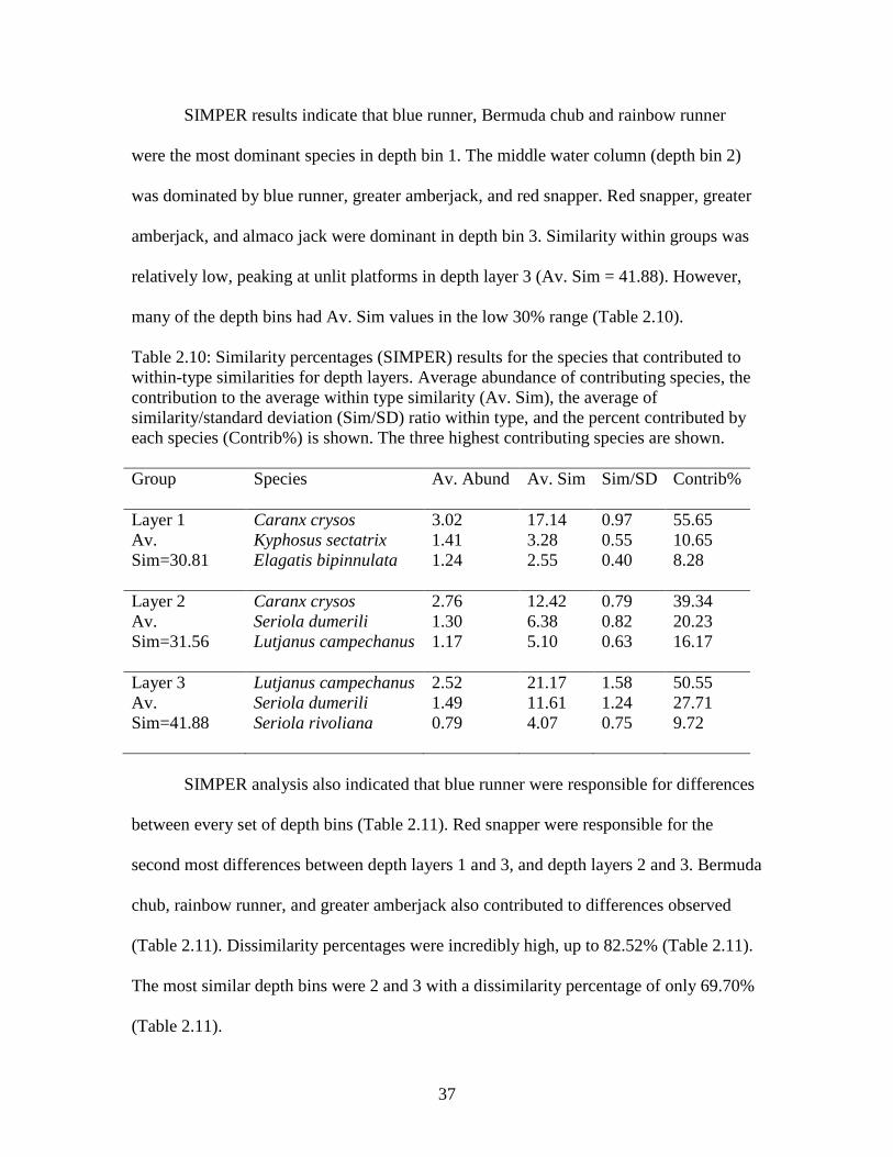
Table 2.10: Similarity percentages (SIMPER) results for the species that contributed

to within-type similarities for depth layers. Average abundance of contributing species, the contribution to the average within type similarity (Av. Sim), the average of similarity/standard deviation (Sim/SD) ratio within type, and the percent contributed by each species (Contrib%) is shown. The three highest contributing species are shown…………………………………………………..37

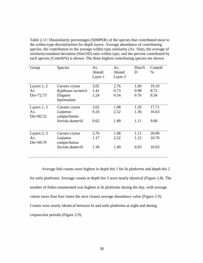
Table 2.11: Dissimilarity percentages (SIMPER) of the species that contributed most

to the within-type dissimilarities for depth layers. Average abundance of contributing species, the contribution to the average within type similarity (Av. Sim), the average of similarity/standard deviation (Sim/SD) ratio within type, and the percent contributed by each species (Contrib%) is shown. The three highest contributing species are shown…………………………………………..38

Table 3.1: Platform demographics. Provided by BSEE (2015)………………………….52

Table 3.2: ANOVA table of Type III Fixed Effects indicating the significance of various effects and interactions on observed mean volume backscatter (MVBS).

Significance was set at α=0.05. Model DF = model degrees of freedom. Error DF = error degrees of freedom…………………………………………………..63 Table A.1: A list of all species observed over the course of the study including MaxN

values, percent the species comprised of the total MaxN (%), number of surveys for which the species was present, and percent of surveys the species was viewed (%)……………………………………………………………………….84

vii

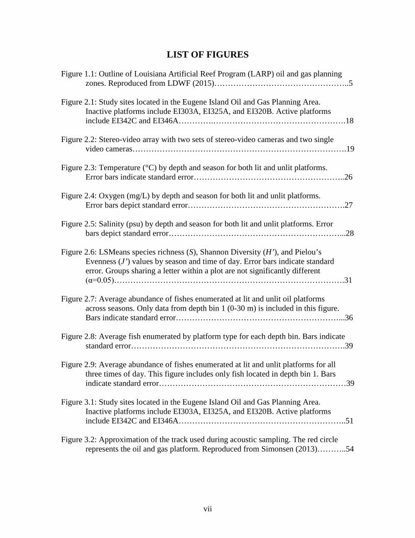
LIST OF FIGURES Figure 1.1: Outline of Louisiana Artificial Reef Program (LARP) oil and gas planning

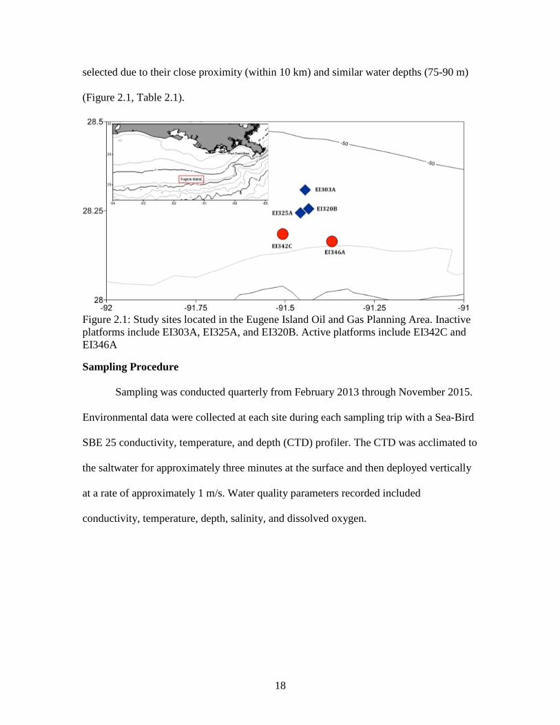
zones. Reproduced from LDWF (2015)…………………………………………..5 Figure 2.1: Study sites located in the Eugene Island Oil and Gas Planning Area.

Inactive platforms include EI303A, EI325A, and EI320B. Active platforms include EI342C and EI346A………….………………………………………….18

Figure 2.2: Stereo-video array with two sets of stereo-video cameras and two single

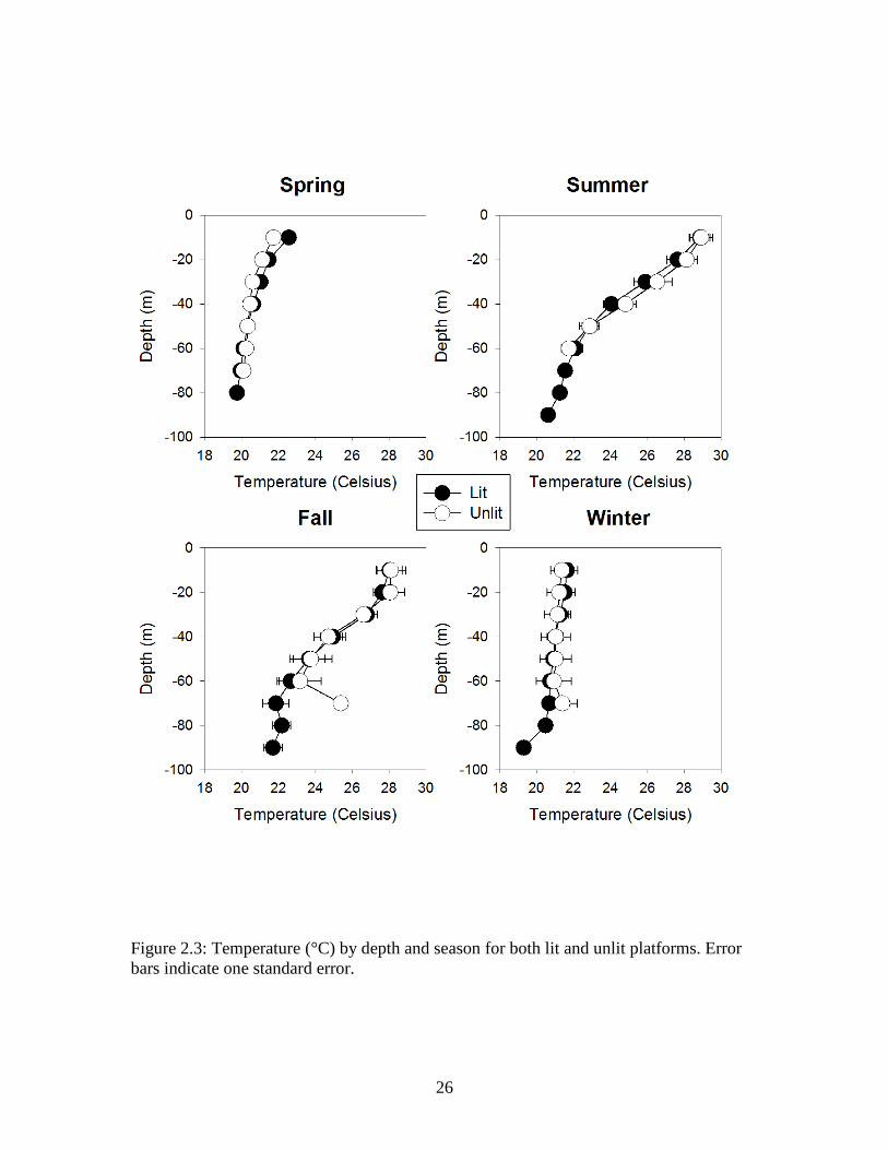
video cameras…………………………………………………………………….19 Figure 2.3: Temperature (°C) by depth and season for both lit and unlit platforms.

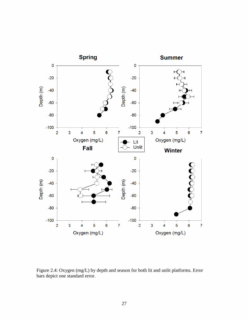
Error bars indicate standard error………………………………………………..26 Figure 2.4: Oxygen (mg/L) by depth and season for both lit and unlit platforms. Error bars depict standard error………………………………………………….27 Figure 2.5: Salinity (psu) by depth and season for both lit and unlit platforms. Error

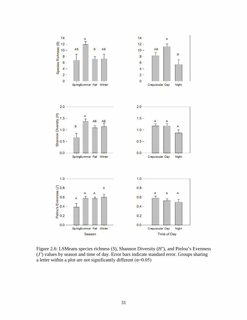
bars depict standard error………………………………………………………...28 Figure 2.6: LSMeans species richness (S), Shannon Diversity (H’), and Pielou’s

Evenness (J’) values by season and time of day. Error bars indicate standard error. Groups sharing a letter within a plot are not significantly different (α=0.05)………………………………………………………………………….31

Figure 2.7: Average abundance of fishes enumerated at lit and unlit oil platforms

across seasons. Only data from depth bin 1 (0-30 m) is included in this figure. Bars indicate standard error……………………………………………………...36

Figure 2.8: Average fish enumerated by platform type for each depth bin. Bars indicate

standard error…………………………………………………………………….39 Figure 2.9: Average abundance of fishes enumerated at lit and unlit platforms for all

three times of day. This figure includes only fish located in depth bin 1. Bars indicate standard error……………………………………………………………39

Figure 3.1: Study sites located in the Eugene Island Oil and Gas Planning Area.

Inactive platforms include EI303A, EI325A, and EI320B. Active platforms include EI342C and EI346A……………………………………………………..51

Figure 3.2: Approximation of the track used during acoustic sampling. The red circle

represents the oil and gas platform. Reproduced from Simonsen (2013)………..54

viii

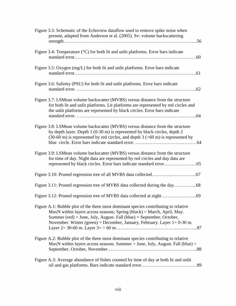
Figure 3.3: Schematic of the Echoview dataflow used to remove spike noise when present, adapted from Anderson et al. (2005). Sv: volume backscattering strength…………………………………………………………………………...56

Figure 3.4: Temperature (°C) for both lit and unlit platforms. Error bars indicate

standard error…………………………………………………………………….60 Figure 3.5: Oxygen (mg/L) for both lit and unlit platforms. Error bars indicate

standard error…………………………………………………………………….61 Figure 3.6: Salinity (PSU) for both lit and unlit platforms. Error bars indicate

standard error. …………………………………………………………………...62 Figure 3.7: LSMean volume backscatter (MVBS) versus distance from the structure

for both lit and unlit platforms. Lit platforms are represented by red circles and the unlit platforms are represented by black circles. Error bars indicate standard error. ………………………………………….………………………..64

Figure 3.8: LSMean volume backscatter (MVBS) versus distance from the structure

by depth layer. Depth 1 (0-30 m) is represented by black circles, depth 2 (30-60 m) is represented by red circles, and depth 3 (>60 m) is represented by blue circle. Error bars indicate standard error. ………………………….………64

Figure 3.9: LSMean volume backscatter (MVBS) versus distance from the structure

for time of day. Night data are represented by red circles and day data are represented by black circles. Error bars indicate standard error…………………65

Figure 3.10: Pruned regression tree of all MVBS data collected………………………..67

Figure 3.11: Pruned regression tree of MVBS data collected during the day…………...68

Figure 3.12: Pruned regression tree of MVBS data collected at night…………………..69

Figure A.1: Bubble plot of the three most dominant species contributing to relative MaxN within layers across seasons; Spring (black) = March, April, May. Summer (red) = June, July, August. Fall (blue) = September, October, November. Winter (green) = December, January, February. Layer 1= 0-30 m. Layer 2= 30-60 m. Layer 3= > 60 m……………………………………………..87

Figure A.2: Bubble plot of the three most dominant species contributing to relative MaxN within layers across seasons. Summer = June, July, August. Fall (blue) =

September, October, November………………………………………………….88 Figure A.3: Average abundance of fishes counted by time of day at both lit and unlit

oil and gas platforms. Bars indicate standard error………………………………89

ix

ABSTRACT

The northern Gulf of Mexico (GOM) contains approximately 2,500 oil and gas

platforms, resulting in one of the largest de facto artificial reef systems in the world. As

of 2013, 1,227 additional structures had ceased to produce oil and gas and have been

decommissioned and removed. While active platforms are lit by high-pressure mercury

vapor lights, inactive platforms are only minimally lit for navigation. The positively

phototaxic behavior of many fish species causes lit oil platforms to act as fish attraction

devices, especially at night. Though a variety of fish species have been reported near

these structures, changes in fish abundance, biomass, and species composition in

response to artificial light regimes has not been studied thoroughly. Hydroacoustic and

video surveys were conducted at two lit and three unlit oil and gas platforms located

approximately 130 km off the coast of Louisiana. The goal of this study was to examine

the effect of artificial lighting on fish community composition and spatial distribution

during the day, night, and during crepuscular periods.

Fish abundance changed with depth, season, time of day, and type of platform

(lit/unlit), with blue runner (Caranx crysos) as the dominant species at both platform

types. Species richness varied with season and time of day, with highest values observed

in the summer and during the day. Hydroacoustic surveys were utilized to determine the

spatial distribution of fish biomass (MVBS, Sv), which was largely concentrated near the

structure and decreased rapidly with distance away from the platform. Platform type did

not significantly impact fish biomass. Fish MVBS was highest in depth layer 3 (>60 m)

and lowest in depth layer 1 (0-30 m), particularly at night. Regression trees showed a

clear area of influence within 45 – 70 m horizontal distance around the structure, as well

x

as fish avoidance behavior of the surface waters (< 9 m). These results suggest that

though fishes are attracted to the vertical relief of the structure, they are actively avoiding

the artificial light field due to nocturnal predation pressure.

1

CHAPTER 1: GENERAL INTRODUCTION

The northern Gulf of Mexico (GOM) currently contains approximately 2,500 oil

and gas platforms, resulting in one of the largest de facto artificial reef systems in the

world (Stanley and Wilson 2000a, b). The first commercially successful offshore

platform was installed by Kerr-McGee on Ship Shoal in 1947, approximately 17 km off

the coast of Louisiana. Since then, construction of new platforms has occurred primarily

off Louisiana (81%) and Texas (14%) (Dauterive 2000, Franks 2000). In total, over 7,000

oil and gas platforms have been constructed in the GOM from 1947 to present day

(LARP 2015). The highest number standing at any given time was 4052 in 2001 (Doug

Peter, Pers. comm.1).

Platforms are outfitted with high-pressure sodium or mercury vapor lights that

operate from dusk to dawn. Additionally, active platforms periodically may produce a

natural gas flare, which burns off petroleum byproducts (Keenan et al. 2007). The

positive phototaxic behavior of many fish species, as well as the vertical relief provided

by the structure, causes oil and gas platforms to act as fish attraction devices (FADs),

especially at night (Simonsen 2013). Though not intended to function as artificial reefs,

these structures secondarily serve to increase the amount of hard substrate and vertical

relief in the GOM, providing aggregation points for fishes and additional habitat for

sessile organisms (Shinn 1974, Scarborough Bull and Kendall 1994, Cox et al. 1996,

Daigle et al. 2013). The northern Gulf of Mexico covers nearly 78,328 km2, yet only

3.3% (2,700 km2) is natural reef habitat (Parker et al. 1983). Only one-third of this hard

1 Doug Peter, Bureau of Safety and Environmental Enforcement, August 2014

2

bottom substrate exists off the coasts of Louisiana and Texas, where 99% of platforms

are located (GMFMC 1989).

Oil and gas platforms contribute an additional 12.1 km2 of hard substrate to the

GOM and are unique in that they provide a continuous vertical link between the photic

zone and benthos (Gallaway and Lewbel 1982, Stanley and Wilson 1996, 2000a). This

additional hard bottom habitat supports a fish community that differs greatly from that

which occurs on the adjacent natural muddy substrate, including many recreationally and

commercially important species such as snappers [red (Lutjanus campechanus),

vermillion (Rhomboplites aurorubens)], groupers [gag (Mycteroperca microlepis), scamp

(Mycteroperca phenax), Warsaw (Epinephelus nigritus)], pelagics [greater amberjack

(Seriola dumerili), king mackerel (Scomberomorus cavalla)], and sharks [sandbar

(Carcharhinus plumbeus), silky (Carcharhinus falciformis), Atlantic sharpnose

(Rhizoprionodon terraenovae), bull (Carcharhinus leucas), greater hammerhead

(Sphyrna mokarran)] as well as many other fish and invertebrate species (Scarborough

Bull and Kendall 1994). Due to their economic and ecological importance, these

structures are recognized by every GOM state as vital reef habitat and legislation is in

place that allows for the conversion of obsolete structures into state-managed artificial

reefs (Scarborough Bull and Kendall 1994). To help resource managers better understand

the role of oil and gas platforms as artificial reefs, many studies have been published that

focus on the surrounding fish abundance and species composition.

The earliest research on oil and gas platforms as artificial reefs was encouraged

by the oil industry itself. Energy companies quickly realized that the cost of scrapping

the metal jackets was simply not in their best economic interest. Shinn (1974), a marine

3

specialist with Shell Oil Company, commented that the average removal cost of an oil

platform at that time could exceed nearly $2,000,000 per platform. To date, cumulative

removal costs of decommissioned platforms have exceeded $1,000,000,000 (Lukens

1997). Therefore, Shinn (1974) suggested that some platforms should remain on the

continental shelf as artificial reef habitat after oil production had ceased. He noted that

platforms serve to provide vertical relief and hard substrate, do not impede the flow of

water, and can promote fishing success for recreational and commercial anglers (Shinn

1974).

However, researchers quickly noted that while platforms served to attract reef-

associated fishes, they provided inferior habitat to natural reefs (Rooker et al. 1997,

Schroeder et al. 2000, Glenn 2014, Schwartzkopf 2014). Additionally, comparisons of

fish communities around oil and gas platforms and naturally occurring reefs have shown

significantly greater biodiversity on natural reefs (Sonnier et al. 1976, Rooker et al. 1997,

Langland 2015).

Most oil platforms are dominated by a few key species that utilize the artificial

reef year-round and lower abundances of migratory species exhibiting low site fidelity

(Stanley and Wilson 2000a). For instance, Rooker et al. (1997) found that the community

structure of fishes at artificial reef platforms was dominated (>50%) by midwater pelagic

species such as carangids and scombrids, whereas at the natural reefs, these species

accounted for <1% of individuals. Sonnier et al. (1976) suggested that due to limited

epifaunal growth on platforms and low habitat complexity, the artificial reefs lacked

sufficient niche breath to support the vast biodiversity found on natural reefs. Schroeder

et al. (2000) calculated that the average habitat value of an oil and gas platform in the

4

Southern California Bight was 42% lower than that for natural reefs, suggesting that

while platforms may act as a fish attraction device for large pelagic species, the metal

jackets provide inferior habitat for some small, reef-dependent species that rely on highly

complex substrates for shelter.

In comparison, natural reefs such as the Flower Garden Banks National Marine

Sanctuary are dominated by highly rugose habitats with high cover by stony corals that

provide ideal refuge from predation for small, reef-associated fishes. Natural reefs also

support higher relative abundance and species diversity, with most fishes being small,

reef-dependent taxa (Rooker et al. 1997, Hernandez et al. 2003). Additionally, a

comparison of fishes at standing platforms versus natural reef habitat on the shelf edge

banks off Louisiana showed that at natural habitats individuals tend to be older

(Kormanec 2015), have greater reproductive potential (Glenn 2014), and are in better

nutritional condition due to a more varied and calorie rich diet than their platform

counterparts (Schwartzkopf 2014).

Despite questions regarding the value of platforms as artificial reef habitat, the

Louisiana Fishing Enhancement Act created the Louisiana Artificial Reef Program

(LARP) in 1986, which seeks to convert “obsolete, nonproductive offshore oil and gas

platforms [into] artificial reefs to support marine habitat” (BSEE 2015). Current federal

regulations dictate that obsolete oil platforms must be removed from the continental shelf

within one year from the lease termination. The LARP offers an alternative for platforms

that meet certain specifications regarding their location, ecological importance, and cost

of removal. Structures close to shore are generally rejected as they are easy to tow back

to scrapyards and the structure often doesn’t meet clearance requirements for boat traffic.

5

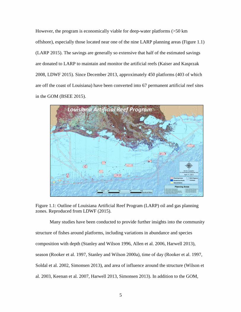
However, the program is economically viable for deep-water platforms (>50 km

offshore), especially those located near one of the nine LARP planning areas (Figure 1.1)

(LARP 2015). The savings are generally so extensive that half of the estimated savings

are donated to LARP to maintain and monitor the artificial reefs (Kaiser and Kasprzak

2008, LDWF 2015). Since December 2013, approximately 450 platforms (403 of which

are off the coast of Louisiana) have been converted into 67 permanent artificial reef sites

in the GOM (BSEE 2015).

Figure 1.1: Outline of Louisiana Artificial Reef Program (LARP) oil and gas planning zones. Reproduced from LDWF (2015).

Many studies have been conducted to provide further insights into the community

structure of fishes around platforms, including variations in abundance and species

composition with depth (Stanley and Wilson 1996, Allen et al. 2006, Harwell 2013),

season (Rooker et al. 1997, Stanley and Wilson 2000a), time of day (Rooker et al. 1997,

Soldal et al. 2002, Simonsen 2013), and area of influence around the structure (Wilson et

al. 2003, Keenan et al. 2007, Harwell 2013, Simonsen 2013). In addition to the GOM,

6

fish communities around oil platforms have been sampled worldwide, including Australia

(Pradella et al. 2014), the Mediterranean Sea (Consoli et al. 2013), the Adriatic Sea (Fabi

et al. 2002, Fabi et al. 2004, Scarcella et al. 2011), the North Sea (Soldal et al. 2002), and

off the coast of California (Bascom et al. 1976, Schroeder et al. 2000) Due to the

inherently stochastic nature of fish populations and the myriad of environmental factors

that impact their distribution, it is difficult to generalize and extrapolate these localized

results to the greater GOM as a whole, especially those conducted in other seas.

Additionally, platforms are notoriously difficult to sample due to the size and depth of the

structures, as well as their distance offshore.

However, over fifty years of study, some general conclusions can be drawn.

Firstly, fishes vertically stratify throughout the water column, following family- and even

species-specific preferences. The top portion of the water column (<30 m) contains

runners and jacks (fam. Carangidae), chubs (fam. Kyphosidae), coastal sharks (fam.

Carcharhinidae), and barracudas (fam. Sphyraenidae). The middle water column (30 – 60

m) is a transition zone containing both large jacks (Carangidae) and snappers (fam.

Lutjanidae). The deepest waters (>60 m) contain primarily snappers (Lutjanidae) and

groupers (fam. Serranidae, fam. Epinephelinae) (Rooker et al. 1997, Stanley and Wilson

2000b, Allen et al. 2006, Reynolds 2015). However, it is possible that these stratifications

can change at night or under varying light regimes.

Additionally, fish biomass is generally concentrated within the structure itself or

within a halo-shaped area of influence around the platform. The size of this area is still

highly debated but has been found to extend up to 100 m, with biomass decreasing with

increasing distance from the structure (Soldal et al. 2002, Simonsen 2013). Most studies

7

cite this halo of fish abundance to be within 20 – 100 meters of the structure, depending

upon reef size (Stanley and Wilson 1996, 1997, 2000b, Fabi and Sala 2002, Boswell et al.

2010).

Metal jackets are large, prolific, and stable, which makes them ideal artificial

reefs. In fact, steel jackets are so stable that Quigel and Thorton (1989) estimated that

they could retain their original structure for at least 300 years. However, the effectiveness

and quality of these platforms as fish habitat needs to be examined. While it has been

shown that fish are attracted to vertical relief (Stanley and Wilson 1991, 1996, Simonsen

2013), they are also highly phototaxic. Fishes are attracted to mercury vapor lights, with

each species and each life stage exhibiting a unique response to varying light thresholds

(Nemeth and Anderson 1992). As artificial light increases, fish have been shown to

establish nocturnal schools in an effort to reduce predation risk (Nightingale et al. 2005).

The late night “antipredator window” of relative safety is often either reduced or even

eliminated as surface lighting aids predators in identifying prey from below.

Additionally, altering the natural illumination regime changes the size of prey being

consumed, as predators are more likely to visually detect larger individuals (Blaxter

1980). It is hypothesized that the artificial lighting of oil and gas platforms in the GOM

could have drastic effects on the nocturnal landscape of the region.

The goal of this study was to compare and describe fish communities at lit versus

unlit platforms, focusing on the effect of light and other environmental variables. Two

active and three inactive platforms within the Eugene Island (EI) Oil and Gas Lease

Planning Area were chosen as study sites. In an effort to conduct unbiased, non-

destructive, and accurate surveys, both mobile hydracoustics and video sampling

8

techniques were successfully implemented for this study. Chapter 2 of this thesis

examines fish assemblage structure around lit and unlit platforms using baited remote

underwater video (BRUV) techniques. BRUVs have been deployed in previous studies in

the GOM (Gledhill et al. 1996, Gledhill et al. 2005) and they are not depth limited,

allowing for efficient, standardized sampling at a variety of depths, habitats, and

environmental conditions.

Chapter 3 examines the spatial and temporal distribution of nektonic biomass

around lit and unlit oil and gas platforms using mobile hydroacoustic surveys.

Hydroacoustics is a popular technique for rapidly assessing acoustic biomass, fish

density, distribution, and area of influence around standing platforms and artificial

structures in the GOM (Stanley and Wilson 1996, 2000a, 2000b, Boswell et al. 2010).

Additionally, this technique is not limited by poor visibility and has minimal impact on

fish behavior, resulting in an accurate “snapshot” of fish biomass and density. The

combination of BRUVs and mobile hydroacoustics allowed me to gain a better

understanding of how light impacts fish community structure and biomass around lit and

unlit oil and gas platforms.

LITERATURE CITED Allen, Y., K. Boswell, M. Miller, D. Nieland, and C. Wilson. 2006. Effects of Depth,

Location, and Habitat Type on Relative Abundance and Species Composition of Fishes Associated with Petroleum Platforms and Sonnier Bank in the Northern Gulf of Mexico. Page 85 in M. M. S. U.S. Dept. of the Interior, Gulf of Mexico OCS Region, editor. New Orleans, LA.

Bascom, W., A. J. Mearns, and M. D. Moore. 1976. A biological survey of oil platforms

in the Santa Barbara Channel. Journal of Petroleum Technology 28(11):1280-1284.

Blaxter, J. H. S. 1980. Vision and feeding of fishes. Pages 32-56 in J.E. Bardach, J.J.

Magnuson, R.C. May, and J.M. Reinhart, editors. Fish behavior and its use in the

9

capture and culture of fishes. ICLARM Conference Proceedings 5, International Center for Living Aquatic Resources Management, Manila, Philippines.

Boswell, K. M., R. J. D. Wells, J. H. Cowan Jr, and C. A. Wilson. 2010. Biomass,

density, and size distributions of fishes associated with a large-scale artificial reef complex in the Gulf of Mexico. Bulletin of Marine Science 86:879-889.

Bureau of Safety and Environmental Enforcement (BSEE). 2015. Platform/Rig

Information. http://www.data.bsee.gov/homepg/data_center/platform/platform.asp. Last accessed June 10, 2015.

Consoli, P., T. Romeo, M. Ferraro, G. Sarà, and F. Andaloro. 2013. Factors affecting fish

assemblages associated with gas platforms in the Mediterranean Sea. Journal of Sea Research 77:45-52.

Cox, S. A., C. R. Beaver, Q. R. Dokken, and J. Rooker. 1996. Diver-based underwater

survey techniques used to assess fish populations and fouling community development on offshore oil and gas platform structures. Pages 101-105 in Methods and Techniques of Underwater Research.

Daigle, S. T. 2013. What Is the Relative Importance of Phytoplankton and Attached

Macroalgae and Epiphytes to Food Webs on Offshore Oil Platforms?. Marine and Coastal Fisheries: Dynamics, Management, and Ecosystem Science 5:53-64.

Dauterive, L. 2000. Rigs-To-Reefs policy, progress, and perspective. U.S. Department of

the Interior, Minerals Management Service, Gulf of Mexico OCS Region. OCS Report MMS 2000-073.

Fabi, G., and A. Sala. 2002. An assessment of biomass and diel activity of fish at an

artificial reef (Adriatic Sea) using a stationary hydroacoustic technique. ICES Journal of Marine Science: Journal du Conseil 59:411-420.

Fabi, G., F. Grati, M. Puletti, and G. Scarcella. 2004. Effects on fish community induced

by installation of two gas platforms in the Adriatic Sea. Marine Ecology Progress Series 273:187-197.

Franks, J. S. 2000. Pelagic fishes at petroleum platforms in the Northern Gulf of Mexico;

diversity, interrelationships, and perspective.in Pêche thonière et dispositifs de concentration de poissons, Caribbean-Martinique, 15-19 Oct 1999.

Gallaway, B. J., and G. S. Lewbel. 1982. Ecology of petroleum platforms in the

northwestern Gulf of Mexico: a community profile. LGL Ecological Research Associates, Inc., Bryan, TX (USA).

10

Gledhill, C. T., J. Lyczkowski-Shultz, K. Rademacher, E. Kargard, G. Crist, and M. A. Grace. 1996. Evaluation of video and acoustic index methods for assessing reef-fish populations. ICES Journal of Marine Science: Journal du Conseil 53:483-485.

Gledhill, C. T., K. R. Rademacher, and P. Felts. SEAMAP Reef Fish Survey of Offshore

Banks. 2005. Pages 38-39 in Somerton, D. A. and C. T. Glendhill (editors). Report of the National Marine Fisheries Service Workshop on Underwater Video Analysis. U.S. Dep. Commerce, NOAA Tech. Memo. NMFS-F/SPO-68.

Glenn, H. D. 2014. Does Reproductive Potential of Red Snapper in the Northern Gulf of

Mexico Differ Among Natural and Artificial Habitats? MS Thesis. Louisiana State University, Baton Rouge.

Gulf of Mexico Fishery Management Council (GMFMC). 1989. Ammendment 1 to the

reef fish fishery management plan. Tampa, FL. 456 pages. Harwell, G. E. 2013. Acoustic biomass of fish associated with an oil and gas platform

before, during and after "reefing" it in the northern Gulf of Mexico. MS Thesis. Louisiana State University, Baton Rouge.

Hernandez, J., Frank J, R. F. Shaw, J. S. Cope, J. G. Ditty, T. Farooqi, and M. C.

Benfield. 2003. The across-shelf Larval, postlarval, and juvenile fish assemblages collected at offshore oil and gas platforms west of the Mississippi River delta. Pages 39-72 in D.R. Stanley and A. Scarborough-Bull, editors. Fisheries, reefs, and offshore development. American Fisheries Society, Symposium 36, Bethesda, Maryland

Kaiser, M. J., and R. A. Kasprzak. 2008. The impact of the 2005 hurricane season on the

Louisiana Artificial Reef Program. Marine Policy 32:956-967. Keenan, S. F., M. C. Benfield, and J. K. Blackburn. 2007. Importance of the artificial

light field around offshore petroleum platforms for the associated fish community. Marine Ecology Progress Series 331:219-231.

Kormanec, M. 2015. Otoliths then and now: a study of ancient and modern fish

populations in Louisiana's coastal waters. Louisiana State University, Baton Rouge, LA.

Langland, T. 2015. Fish assemblage structure, distribution, and trophic ecology at

northwestern Gulf of Mexico banks. Ph.D. dissertation. Louisiana State University, Baton Rouge, LA.

Louisiana Artificial Reef Program (LARP). 2015. Artificial Reef Program.

http://www.wlf.louisiana.gov/fishing/artificial-reef-program. Last accessed December 8, 2015.

11

Louisiana Department of Fish and Wildlife (LDWF). 2015. Louisiana Artificial Reef Program (LARP). Artificial Reef Program. http://www.wlf.louisiana.gov/fishing/artificial-reef-program. Last accessed June 5, 2015.

Lukens, R. R. 1997. Oil and gas platforms. Pages 82 – 91 in Guidelines for Marine

Artificial Reef Materials. Gulf States Marine Fisheries Commission. Nemeth, R. S., and J. J. Anderson. 1992. Response of juvenile coho and chinook salmon

to strobe and mercury vapor lights. North American journal of fisheries management 12:684-692.

Nightingale, B., T. Longcore, and C. A. Simenstad. 2005. Artificial Night Lighting and

Fishes.in T. Longcore and C. Rich, editors. Ecological Consequences of Artificial Night Lighting. Island Press, Washington.

Parker, R., D. R. Colby, and T. Willis. 1983. Estimated amount of reef habitat on a

portion of the US South Atlantic and Gulf of Mexico continental shelf. Bulletin of Marine Science 33:935-940.

Pradella, N., A. M. Fowler, D. J. Booth, and P. I. Macreadie. 2014. Fish assemblages

associated with oil industry structures on the continental shelf of north-western Australia. Journal of Fisheries Biology 84:247-55.

Quigel, J. C. and W. L. Thorton. 1989. Rigs to Reefs – A case history. Pages 77-83 in

V.C. Reggio, editor. Petroleum Structures as Artificial Reefs: A Compendium. OCS MMS 89-0021. U.S. Department of the Interior, Mineral Management Service, Gulf of Mexico OCS Region, New Orleans, LA.

Reynolds, E. 2015. Fish biomass and community structure around standing and toppled

oil and gas platforms in the northern Gulf of Mexico using hydroacoustic and video surveys. Louisiana State University, Baton Rouge, LA.

Rooker, J., Q. Dokken, C. Pattengill, and G. Holt. 1997. Fish assemblages on artificial

and natural reefs in the Flower Garden Banks National Marine Sanctuary, USA. Coral Reefs 16:83-92.

Scarborough Bull, A., and J. J. Kendall, Jr. 1994. An indication of the process: offshore

platforms as artificial reefs in the Gulf of Mexico. Bulletin of Marine Science 55:1086-1098.

Scarcella, G., F. Grati, and G. Fabi. 2011. Temporal and spatial variation of the fish

assemblage around a gas platform in the Northern Adriatic Sea, Italy. Turkish Journal of Fisheries and Aquatic Sciences 11:433-444.

12

Schroeder, D. M., A. J. Ammann, J. A. Harding, L. A. MacDonald, and W. T. Golden. 2000. Relative habitat value of oil and gas production platforms and natural reefs to shallow water fish assemblages in the Santa Maria Basin and Santa Barbara Channel, California. Pages 493-498 in Proc. Fifth Calif. Islands Symp.

Schwartzkopf, B. D. 2014. Assessment of Habitat Quality for Red Snapper, Lutjanus

campechanus, in the Northwestern Gulf of Mexico: Natural vs. Artificial Reefs. MS Thesis. Louisiana State University, Baton Rouge.

Shinn, E. A. 1974. Oil structures as artificial reefs. Pages 91-96 in Proceedings of an

international conference on artificial reefs. Texas A&M University, Houston, Texas.

Simonsen, K. A. 2013. Reef fish demographics on Louisiana artificial reefs: the effects of

reef size on biomass distribution and foraging dynamics. Ph.D. dissertation. Louisiana State University, Baton Rouge.

Soldal, A. V., I. Svellingen, T. Jørgensen, and S. Løkkeborg. 2002. Rigs-to-reefs in the

North Sea: hydroacoustic quantification of fish in the vicinity of a “semi-cold” platform. ICES Journal of Marine Science: Journal du Conseil 59(suppl):S281-S287.

Sonnier, F., J. Teerling, and H. Dickson Hoese. 1976. Observation on the offshore reef

and platform fish fauna of Louisiana. Copeia 1976:105-111. Stanley, D. R., and C. A. Wilson. 1991. Factors affecting the abundance of selected fishes

near oil and gas platforms in the northern Gulf of Mexico. Fishery Bulletin 89:149-159.

Stanley, D. R., and C. A. Wilson. 1996. Abundance of fishes associated with a petroleum

platform as measured with dual-beam hydroacoustics. ICES Journal of Marine Science: Journal du Conseil 53:473-475.

Stanley, D. R., and C. A. Wilson. 1997. Seasonal and spatial variation in the abundance

and size distribution of fishes associated with a petroleum platform in the northern Gulf of Mexico. Canadian Journal of Fisheries and Aquatic Sciences 54:1166–1176.

Stanley, D. R., and C. A. Wilson. 2000a. Variation in the density and species composition

of fishes associated with three petroleum platforms using dual beam hydroacoustics. Fisheries Research 47:161-172.

Stanley, D. R., and C. A. Wilson. 2000b. Seasonal and spatial variation in the biomass

and size frequency distribution of fish associated with oil and gas platforms in the northern Gulf of Mexico. OCS Study MMS 2000-005:252.

13

Wilson, C. A., A. Pierce, and M. W. Miller. 2003. Rigs and Reefs: a comparison of the fish communities at two artificial reefs, a production platform, and a natural reef in the northern Gulf of Mexico. Mineral Management Service, OCS Study MMS 2003- 009, New Orleans, 95 p.

14

CHAPTER 2: CHARACTERIZATION OF COMMUNITY STRUCTURE AROUND ACTIVE AND DECOMMISSIONED OIL

AND GAS PLATFORMS IN THE NORTHERN GULF OF MEXICO

INTRODUCTION In an effort to satisfy the global need for oil, over 2,500 oil and gas platforms are

currently located in the Gulf of Mexico (GOM), accounting for 30% of the nation’s

domestic oil production (BSEE 2015). Artificial reefs formed by oil and gas platforms are

important to many stakeholders as they attract and concentrate recreationally and

commercially important fish species. By 1979, over 99% of all offshore recreational

charter boats and commercial fishing vessels in Louisiana waters fished at platforms

(Dugas et al. 1979). Today, nearly $1.5 million annually is spent on private charter boats

for recreational fishing off the Louisiana coast (Hiett and Milon 2002). Due to their

economic and ecological importance, these structures are recognized by every GOM state

as vital reef habitat and legislation is in place that allows for the conversion of obsolete

structures into state-managed artificial reefs (Scarborough Bull and Kendall 1994).

To effectively study these artificial reef structures, efficient, standardized

sampling methodology must be employed. Today, many studies utilize baited remote

underwater video (BRUV) techniques as a non-extractive method of monitoring fishes in

situ (Cappo et al. 1999, 2006, Wells 2007). BRUVs sidestep the potential risks involved

with SCUBA diving and are not depth limited, allowing for convenient sampling at a

variety of depths, habitats, and environmental conditions. Additionally, stereo-video

arrays provide a permanent record of observations, resulting in less subjective data, while

the ability to watch and rewatch footage increases both accuracy and precision of length

measurements. Whereas in situ diver data were often erroneous with regards both to fish

15

length and to distance from transect, computer programs, including the popular SeaGIS

EventMeasure™ system, are accurate to within 1 – 2% of a fish’s true length and can be

used to measure fishes in excess of 9 meters from the camera (Cappo et al. 2006).

Additionally, stereo-video systems allow the researcher to view video segments multiple

times, freezing each frame as needed to obtain the best view of a particular fish and thus

increasing accuracy of both identification and measurement.

Prior to stereo-cameras, SCUBA divers had simply counted fish, recording

density, approximate length, and species composition on dive slates. While this method

was successful for habitats in which species diversity and fish abundance were relatively

low, it simply wasn’t feasible for highly diverse habitats. Even the most experienced

divers consistently underestimated population densities while overestimating the length

of small fish and underestimating the length of large fish (Harvey et al. 2002, Harvey et

al. 2007). Additional sources of bias arose, which questioned the number of species that

can be accurately counted at one time, swimming speed of the diver, and the behavior of

fish toward divers. All of these factors can impact the accuracy of SCUBA surveys and

prevent comparison across studies. Due to these sources of error, BRUVs are the new

standard for sampling fish populations effectively.

There has been much debate in the literature regarding the use of bait as an

attractant for these types of stereo-video arrays. Proponents of baited systems argue that

the bait attracts fish already in the area, thus providing a larger data set and more accurate

assessment of community structure (Watson et al. 2005, Cappo et al. 2006, Stobart et al.

2007). However, many scientists believe this method is flawed and argue that the

resulting video is biased toward either predatory or scavenging species while

16

discriminating against herbivorous or omnivorous species (Harvey et al. 2007). Watson et

al. (2005) compared the effectiveness of three sampling systems: baited and unbaited

remote sampling versus diver-operated systems. They found that the baited video

recorded 33 fish species, while the unbaited video only recorded 23. The divers had the

advantage of being able to enter crevices that were inaccessible to the remote stereo-

video. Therefore, several species were detected on the diver surveys that did not appear in

either of the remote surveys. Despite this, baited remote stereo-video was determined to

produce the highest power results with the fewest replications, making it the preferred

method for studying fish communities. Clearly, baited stereo-video arrays are valuable

tools for fisheries monitoring projects worldwide and can greatly increase our

understanding of aquatic habitats and the animals that call them home.

There has been very little research dedicated to examining the effects of platform

lighting on surrounding fish communities. Active platforms are outfitted with either high-

pressure sodium or mercury vapor lights that operate from dusk to dawn. Additionally,

active platforms periodically may produce a natural gas flare, which burns off petroleum

byproducts (Keenan et al. 2007). The positive phototaxic behavior of many fish species,

as well as the vertical relief provided by the structure, causes oil and gas platforms to act

as fish attraction devices (FADs), especially at night (Simonsen 2013). Keenan et al.

(2007) determined that the light produced by two platforms in the northern GOM

extended more than 10 meters below the sea surface. This may greatly alter the nocturnal

landscape around platforms by creating a halo of light that concentrates both predatory

and planktivorous species, as per results in Blaxter (1980).

17

It is apparent that oil and gas platforms support high fish biomass and density,

including large pelagic fishes such as greater amberjack (Seriola dumerili), great

barracuda (Sphyraena barracuda), and many species of coastal sharks (Stanley and

Wilson 1991, 1996, 1997, Franks 2000, Stanley and Wilson 2000a, b, Boswell et al.

2010). However, little information exists regarding how fish community structure may

vary temporally and spatially in relation to lit and unlit platforms. The goal of this chapter

was to compare the community structure of fishes at lit versus unlit oil and gas platforms

by season, type of structure, and depth by utilizing BRUVS. The working hypothesis was

that there would be greater species richness and abundance at the lit platforms due to the

positive phototaxic behavior of many fish species.

METHODS AND MATERIALS

Study Sites

Five oil and gas platforms located approximately 130 km off the coast of

Louisiana were selected for examining the effects of artificial light on fish community

structure (Figure 2.1). The five platforms were located in the Eugene Island (EI) Oil and

Gas Lease Planning Area, and consisted of two operational lit oil and gas platforms

(hereafter lit) and three decommissioned unlit oil and gas platforms (hereafter unlit).

Active platforms are lit by high-pressure mercury vapor floodlights around the exterior of

the structure, which allows for normal working operations to proceed 24 hours a day. An

additional source of illumination is a natural gas flare stack, which periodically combusts

any natural gas or petroleum byproducts released (Keenan et al. 2007). Unlit platforms

are only minimally lit for the purpose of avoidance by boat traffic. Platforms were

18

selected due to their close proximity (within 10 km) and similar water depths (75-90 m)

(Figure 2.1, Table 2.1).

Figure 2.1: Study sites located in the Eugene Island Oil and Gas Planning Area. Inactive platforms include EI303A, EI325A, and EI320B. Active platforms include EI342C and EI346A

Sampling Procedure

Sampling was conducted quarterly from February 2013 through November 2015.

Environmental data were collected at each site during each sampling trip with a Sea-Bird

SBE 25 conductivity, temperature, and depth (CTD) profiler. The CTD was acclimated to

the saltwater for approximately three minutes at the surface and then deployed vertically

at a rate of approximately 1 m/s. Water quality parameters recorded included

conductivity, temperature, depth, salinity, and dissolved oxygen.

19

Table 2.1: Platform demographics of the two lit and three unlit platforms in the Eugene Island (EI) Oil and Gas Lease Block. Provided by BSEE (2015) and LDWF (2015). Platform Latitude Longitude Type Water

Depth (m)

Year of Installation

Number of Piles

Operating Company

EI346A 28°9’49.00” N 91°22’ 8.19” W Lit 96 2000 4 Fieldwood Energy LLC

EI342C 28°11’3.99” N 91°30’ 23.95” W Lit 87 1986 4 Apache Shelf, Inc.

EI325A 28°14’39.00” N 91°27’ 26.00” W Unlit 78 1989 4 Apache Shelf, Inc.

EI320B 28°15’20.13” N 91°26’ 2.63” W Unlit 77 2006 3 Arena Offshore,

LP

EI303A 28°18' 30.29" N 91° 26' 37.91" W Unlit 69 2005 3 Ridgelake Energy, Inc.

20

Video surveys were conducted during the day, at night, or during crepuscular

periods to provide diurnal, transitional, and nocturnal community structure data. A six-

camera array consisted of a circular metal cage within which two Canon VIXIA HF G10

stereo camera pairs and two single cameras were mounted (Figure 2.2). The stereo

cameras are separated by 70 cm and angled inward at 7 degrees to collect high-resolution

images of nekton distributed around the platforms with maximum area of overlap. Two

single cameras were mounted at right angles affording a nearly 3600 view. Four 50 watt

HID lights (Light Monkey Enterprises LLC, Florida, USA) were mounted to the cage

above each of the single or stereo-camera sets. Each light had a waterproof battery (also

attached to the cage) and provided 5000 Lumen Output with a battery life of

approximately 2 hours. The cage was baited with either Gulf menhaden (Brevoorita

Figure 2.2: Stereo-video array with two sets of stereo-video cameras and two single video cameras.

21

patronus) or chub mackerel (Scomber japonicas). The water column was split into three

depth strata: top, middle, and bottom segments, each accommodating one-third of the

water column: 0-30 m, 30-60 m, and >60 m (hereafter referred to as depth layers 1, 2, and

3 respectively). The cameras recorded at the middle of each depth stratum (i.e. 12.5 m)

for 20 minutes, for a total of one hour per drop.

Data Analysis

EventMeasure software (SeaGIS Pty. Ltd.) was used to identify and enumerate all

species present in the video footage. Identifications were made to the lowest possible

taxonomic level (usually species) and counts were calculated as MaxN (Priede et al.

1994). MaxN is a conservative estimate of the number of fish present during a survey. It

is defined as the maximum number of individuals of a particular species that can be seen

in a single video frame. This method prevents recounting individual fish that may either

swim in and out of the frame or circle the baited cage. First, MaxN was determined for

each individual camera. The largest individual camera MaxN value was selected,

resulting in one MaxN value per depth per species. For biological indices calculations,

MaxN values for each species were summed across depth bins, resulting in one MaxN

value for each species per platform.

The Relative MaxN of an individual species was calculated from MaxN values

averaged over a variable of interest. Relative MaxN was defined by:

Relative MaxN (%) = (Individual species MaxN/total MaxN) x 100

All video data were analyzed with Plymouth Routines in Multivariate Ecological

Research v. 6 (Primer-E software, Primer-E Ltd., Lutton, United Kingdom). The data

were log(x+1) transformed to reduce the impact of highly abundant species and to

22

eliminate zeros from the data. A resemblance matrix was calculated which defined the

zero-adjusted Bray-Curtis similarity between every pair of samples.

Traditional assemblage metrics of evenness, richness, and diversity were

calculated. Species richness (S) was simply expressed as the number of species present in

each survey. Shannon’s diversity index (H’) was expressed as:

𝐻𝐻’ = − Σi 𝑝𝑝i ln 𝑝𝑝i

where pi is the proportional of total individuals belonging to the ith species. Pielou’s

evenness index (J’) was expressed as:

J’ = H’/H’max =H’/logS

where H’ is the observed possible value of Shannon diversity and H’max is the maximum

possible value of Shannon diversity for that survey.

MaxN was analyzed using permutational multivariate analysis of variance

(PERMANOVA) to partition variation among depth, season and lit versus unlit, and

diversity, evenness, and richness were compared across seasons and time of day. All

video data were analyzed with Plymouth Routines in Multivariate Ecological Research v.

6 (Primer-E software, Primer-E Ltd., Lutton, United Kingdom). The MaxN data were

log(x+1) transformed to reduce the impact of highly abundant species. A resemblance

matrix was that calculated which defined the zero-adjusted Bray-Curtis similarity

between every pair of cruises. Traditional assemblage metrics of evenness, richness, and

diversity were calculated for season and time of day. PERMANOVA was conducted with

depth, season, and platform type (lit/unlit) as fixed variables. Originally, the model

included time of day as a fixed variable but was removed to prevent confounding

variables. The null hypothesis was that species abundance did not change either between

23

active and inactive platforms or with time of day. If the community composition around

platforms was significantly different, pairwise tests were computed to determine which

factors were significantly different from each other. To determine which species

contributed the most to the similarity in the community structure between lit and unlit

platforms, a similarity percentages (SIMPER) procedure was performed.

A distance based linear model (DistLM) was performed to test for correlation

between the observed fish community structure and environmental data recorded by the

CTD: temperature (°C) and salinity (PSU). The model with the lowest Akaike

information criterion (AIC) scores was selected. CTD data were plotted as the mean ±

standard deviation at discrete depths (every 10 m, from 0-100 m) to examine differences

in temperature, salinity, and dissolved oxygen with season and depth.

RESULTS Between June 2013 and November 2015, a total of 62 camera-array surveys were

conducted: 30 during the day, 21 during crepuscular periods, and 11 at night. Forty-five

fish species in 20 families were observed (Appendix, Table A.1). Blue runner (Caranx

crysos) was the most abundant species, accounting for 46.34% of individuals observed,

followed by little tunny (Euthynnus alletteratus, 14.86%), and red snapper (Lutjanus

campechanus, 7.84%). Taxa were functionally diverse with planktivorous species (e.g.

rainbow runner Elagatis bipinnulata) through large predators (e.g. Lutjanus spp. and

Carcharhinus spp.) represented.

At lit platforms, 39 species were observed, while only 34 species were observed

at unlit platforms (Table 2.2). Eleven species were identified only at lit platforms, 6

species were identified at only unlit platforms, and 28 species were observed at both

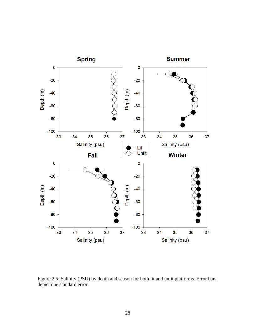
24

types. The CTD profiles indicated a stratified water column with a strong thermocline

and halocline during the summer and early fall. During spring and winter months, the

water column was well mixed. Temperature (°C), dissolved oxygen (mg/L), and salinity

(PSU) showed similar patterns at both lit and unlit platforms (Figures 2.3, 2.4, and 2.5,

respectively).

Table 2.2: List of species observed at unlit and lit oil and gas platforms.

Group Species Scientific Name Max N Average

Max N Standard Deviation

Unlit Blue runner Caranx crysos 168.9 164.0 Platform Red snapper Lutjanus campechanus 22.0 22.3 Bermuda chub Kyphosus sectatrix 15.0 25.3 Greater amberjack Seriola dumerili 11.4 7.0 Horse-eye jack Caranx latus 10.7 28.3 Crevalle jack Caranx hippos 8.2 15.3 Little tunny Euthynnus alletteratus 7.6 22.3 Rainbow runner Elagatis bipinnulata 6.4 10.3 Almaco jack Seriola rivoliana 5.0 6.7 Vermillion snapper Rhomboplites aurorubens 4.2 9.3 Gray snapper Lutjanus griseus 2.9 5.2 Spotfin hogfish Bodianus pulchellus 0.9 4.2 Gray triggerfish Balistes capriscus 0.9 1.5 Lookdown Selene vomer 0.7 3.0 Ocean triggerfish Canthidermis sufflamen 0.7 1.6 Creolefish Paranthias furcifer 0.5 2.7 Bar jack Caranx ruber 0.4 1.5 Silky shark Carcharhinus falciformis 0.4 1.0 Barracuda Sphyraena barracuda 0.4 0.6 Yellow jack Carangoides bartholomaei 0.3 1.2 Spinner shark Carcharhinus brevipinna 0.2 0.7 Great hammerhead Sphyrna mokarran 0.2 0.6 Scamp Mycteroperca phenax 0.2 0.6 Cobia Rachycentron canadum 0.2 0.5 Remora Remora remora 0.1 0.4 Sandbar shark Carcharhinus plumbeus 0.1 0.3 French angelfish Pomacanthus paru 0.06 0.3 Atlantic spadefish Chaetodipterus faber 0.06 0.3 Warsaw grouper Epinephelus nigritus 0.06 0.2 Lionfish Pterois miles 0.06 0.2

25

(Table 2.2 continued)

Group Species Scientific Name Max N Average

Max N Standard Deviation

Unlit Atlantic sharpnose Rhizoprionodon terraenovae 0.03 10.3 Platform Dusky shark Carcharhinus obscurus 0.03 0.2 Bull shark Carcharhinus leucas 0.03 0.2 Giant Manta Ray Manta birostris 0.03 0.2 Lit Blue runner Caranx crysos 151.9 256.8 Platform Little tunny Euthynnus alletteratus 105.3 361.3 Rainbow runner Elagatis bipinnulata 45.3 101.7 Red snapper Lutjanus campechanus 34.0 32.2 Horse-eye jack Caranx latus 30.7 53.3 Bermuda chub Kyphosus sectatrix 19.8 33.2 Greater amberjack Seriola dumerili 9.6 7.5 Crevalle jack Caranx hippos 9.2 18.9 Creolefish Paranthias furcifer 5.9 29.9 Almaco jack Seriola rivoliana 3.4 2.9 Silky shark Carcharhinus falciformis 3.3 4.2 Vermillion snapper Rhomboplites aurorubens 2.6 7.6 Bar jack Caranx ruber 2.3 7.7 Tarpon Megalops atlanticus 1.4 7.2 Ocean triggerfish Canthidermis sufflamen 1.4 2.9 Yellow jack Carangoides bartholomaei 1.1 4.1 Barracuda Sphyraena barracuda 0.9 0.9 Sergeant major Abudefduf saxatilis 0.8 4.3 Gray snapper Lutjanus griseus 0.5 1.3 Scamp Mycteroperca phenax 0.4 1.0 Spotfin hogfish Bodianus pulchellus 0.3 1.7 Queen angelfish Holacanthus ciliaris 0.3 1.1 Spinner shark Carcharhinus brevipinna 0.3 1.0 Blue angelfish Holocanthus bermudensis 0.1 0.5 Gag grouper Mycteroperca microlepis 0.1 0.4 Remora Remora remora 0.1 0.4 Sandbar shark Carcharhinus plumbeus 0.07 0.4 Cobia Rachycentron canadum 0.07 0.4 Lionfish Pterois miles 0.07 0.4 French angelfish Pomacanthus paru 0.07 0.4 Warsaw grouper Epinephelus nigritus 0.07 0.3 Great hammerhead Sphyrna mokarran 0.07 0.3 Longspine porgy Stenotomus caprinus 0.04 0.2

26

Figure 2.3: Temperature (°C) by depth and season for both lit and unlit platforms. Error bars indicate one standard error.

27

Figure 2.4: Oxygen (mg/L) by depth and season for both lit and unlit platforms. Error bars depict one standard error.

28

Figure 2.5: Salinity (PSU) by depth and season for both lit and unlit platforms. Error bars depict one standard error.

29

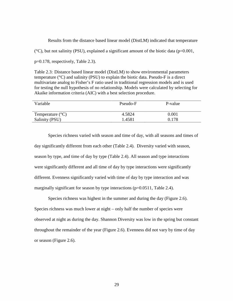
Results from the distance based linear model (DistLM) indicated that temperature

(°C), but not salinity (PSU), explained a significant amount of the biotic data (p=0.001,

p=0.178, respectively, Table 2.3).

Table 2.3: Distance based linear model (DistLM) to show environmental parameters temperature (°C) and salinity (PSU) to explain the biotic data. Pseudo-F is a direct multivariate analog to Fisher’s F ratio used in traditional regression models and is used for testing the null hypothesis of no relationship. Models were calculated by selecting for Akaike information criteria (AIC) with a best selection procedure. Variable Pseudo-F

P-value

Temperature (°C) 4.5824 0.001 Salinity (PSU) 1.4581 0.178

Species richness varied with season and time of day, with all seasons and times of

day significantly different from each other (Table 2.4). Diversity varied with season,

season by type, and time of day by type (Table 2.4). All season and type interactions

were significantly different and all time of day by type interactions were significantly

different. Evenness significantly varied with time of day by type interaction and was

marginally significant for season by type interactions (p=0.0511, Table 2.4).

Species richness was highest in the summer and during the day (Figure 2.6).

Species richness was much lower at night – only half the number of species were

observed at night as during the day. Shannon Diversity was low in the spring but constant

throughout the remainder of the year (Figure 2.6). Evenness did not vary by time of day

or season (Figure 2.6).

30

Table 2.4: Analysis of variance (ANOVA) tests for type, season, time of day, season by type interactions and time of day by type interactions for three diversity indices. Asterisks (*) denotes a significant difference (α = 0.05). Index

Effect F value P-value

Species Richness (S) Type 0.01 0.9131 Season 5.15 0.0035* Time of Day 7.20 0.0018* Season x Type 0.91 0.4451 Time of Day x

Type 0.79 0.4610

Diversity (H’) Type 1.85 0.2286 Season 5.08 0.0039* Time of Day 2.74 0.0743 Season x Type 4.45 0.0077* Time of Day x

Type 3.63 0.0340*

Evenness (J’) Type 4.12 0.1040 Season 2.23 0.0966 Time of Day 1.12 0.3335 Season x Type 2.78 0.0511 Time of Day x

Type 6.82 0.0025*

The PERMANOVA indicated significant differences in fish community structure

between site types and among seasons and depths (p<0.05, Table 2.5). A significant two-

way interaction effect between season and type was found.

31

Figure 2.6: LSMeans species richness (S), Shannon Diversity (H’), and Pielou’s Evenness (J’) values by season and time of day. Error bars indicate standard error. Groups sharing a letter within a plot are not significantly different (α=0.05)

32

Table 2.5: Permutational multivariate analysis of variance (PERMANOVA) source table comparing log(x+1) community structure of fishes within depth layers, seasons, time of day, and between type of structure. Asterisk (*) denotes significant effect (α=0.05). df= degrees of freedom.

Season by Type

In pairwise tests, the spring, fall, and winter significant differences were detected

between platform types (Table 2.6). The community structure around lit platforms varied

with all season combinations except for fall/spring and winter/spring (Table 2.6). The

community structure around unlit platforms varied significantly with all season

combinations (Table 2.6).

SIMPER results indicate that red snapper, blue runner, and greater amberjack

were dominant in many of the season by layer interactions. Other species of importance

included almaco jack (Seriola rivoliana), silky shark (Carcharhinus falciformis), and

horse-eye jack (Caranx latus). Similarity within groups was relatively low, peaking at

unlit platforms in the spring (Av. Sim = 45.88). However, many of the season, platform

type pairings had Av. Sim values in the 20-30% range (Table 2.7).

Variable df Pseudo-F P(perm) Unique perms

Season 3 3.6086 0.001* 999

Type 1 6.6859 0.001* 999

Depth 2 14.598 0.001* 999

Season x Type

3 2.1457 0.005* 999

Season x Depth

6 1.3642 0.079 997

Type x Depth 2 1.4738 0.121 998

33

Table 2.6: Pair-wise tests from PERMANOVA for season by platform type; Asterisk (*) denotes a significant effect (α=0.05). Factor Group t P(perms) Unique Perms Spring Lit, Unlit 2.4710 0.003* 999 Summer Lit, Unlit 1.2782 0.134 998 Fall Lit, Unlit 2.1982 0.001* 998 Winter Lit, Unlit 1.6807 0.011* 998 Unlit Summer, Fall

Summer, Winter Summer, Spring Fall, Winter Fall, Spring Winter, Spring

2.0397 1.6608 1.6954 1.3138 1.2662 1.7555

0.004* 0.009* 0.018* 0.103 0.165 0.010*

999 998 999 998 998 999

Lit Summer, Fall Summer, Winter Summer, Spring Fall, Winter Fall, Spring Winter, Spring

1.8150 1.7088 1.6595 1.6761 1.5215 1.3924

0.004* 0.008* 0.011* 0.004* 0.022* 0.100

997 999 999 997 998 999

Table 2.7: Similarity percentages (SIMPER) results for the species that contributed most to similarities between season and platform type interactions. Shown are average abundances of species within platform type, the contribution to the average within platform type by season similarity (Av. Sim), the average similarity/standard deviation (Sim/SD) ratio within platform type by season, and percent contributed by that species (Contrib %). Only the three most contributing species are shown. Spring = March, April, May, Summer = June, July, August, Fall = September, October, November, Winter = December, January, February. Factor Group Species Av.

Abund Av. Sim

Sim/SD Contrib %

Spring Lit Av. Sim=17.84

Seriola rivoliana Lutjanus campechanus Seriola dumerili

1.10 1.27

0.72

9.41 4.91

3.52

1.00 0.32

0.57

52.77 27.49

19.74

Unlit Av. Sim=54.88

Caranx crysos Lutjanus campechanus Seriola dumerili

3.93 1.63

0.98

27.21 10.18

7.79

1.75 1.28

1.11

49.59 18.55

14.19

Summer Lit Av. Sim=30.22

Caranx crysos Seriola dumerili Lutjanus campechanus

2.44 1.54 1.63

8.82 8.43 5.57

0.75 0.97 0.49

29.18 27.90 18.45

34

(Table 2.7 continued) Factor Group Species Av.

Abund Av. Sim

Sim/SD Contrib %

Unlit Av. Sim=36.07


2.58 1.43 1.56

10.16 6.92 6.07

0.79 1.36 0.70

28.16 19.18 16.84

Fall Lit Av. Sim=24.41

Caranx crysos Lutjanus campechanus Carcharhinus falciformis

1.42

1.10

0.71

5.06

4.62

3.69

0.53

0.44

0.50

20.72

18.92

15.13 Unlit

Av. Sim=31.02


2.57 1.03 1.04

17.41 5.47 4.94

0.75 0.54 0.55

56.11 17.63 15.91

Winter Lit Av. Sim=25.33

Caranx latus Lutjanus campechanus Seriola rivoliana

1.77 1.38

0.71

6.29 4.41

3.92

0.51 0.46

0.86

24.84 17.42

15.50

Unlit Av. Sim=29.88

Lutjanus campechanus Caranx crysos Seriola dumerili

1.31

1.81 1.00

9.50

7.56 6.86

0.68

0.62 0.58

31.81

25.31 22.94

SIMPER analysis indicated that blue runner was the primary species driving

differences for every platform type, season interaction (Table 2.8). Blue runner explained

the most differences in spring but the least in summer (33.79% and 14.16%, respectively,

Table 2.8). Red snapper was the second most dominant species for all platform type,

season combinations except for Winter Unlit and Lit (Table 2.8). Bermuda chub, red

snapper, and greater amberjack also contributed to differences observed (Table 2.8).

Abundances of dominant species were typically higher at unlit platforms, except in the

winter, when lit platforms had a higher abundance of all three dominating species (Table

2.8).

35

Table 2.8: Dissimilarity percentages (SIMPER) results for the species that contributed to the dissimilarity between platform type and season combinations that are significant. Shown are average abundances of species within platform type, the contribution to the average within platform type by season similarity (Av. Dis), the average dissimilarity/standard deviation (Diss/SD) ratio within platform type by season, and percent contributed by that species (Contrib %). Only the three most contributing species are shown. Spring = March, April, May, Summer = June, July, August, Fall = September, October, November, Winter = December, January, February. Group

Species Av. Abund Av. Abund Diss/SD Contrib%

Spring Unlit & Spring Lit Av. Dis=71.82


Spring Unlit 3.93 1.63

1.35

Spring Lit 1.14 1.27

0.72

1.62 1.33

0.94

33.79 15.43

10.52

Summer Lit & Summer Unlit Av. Dis=67.44

Caranx crysos Lutjanus campechanus Kyphosus sectatrix

Summer Unlit 2.58 1.56 1.37

Summer Lit 2.44 1.63 1.09

1.29 1.01 1.02

14.16 11.53 8.48

Fall Unlit & Fall Lit Av. Dis=76.24


Fall Unlit 2.57 1.04

1.03

Fall Lit 1.42 1.10

0.87

1.12 0.97

0.97

21.96 12.99

9.99

Winter Unlit & Winter Lit Av. Dis=76.57

Caranx crysos Caranx latus Lutjanus campechanus

Winter Unlit 1.81 0.85 1.31

Winter Lit 1.89 1.77 1.38

1.08 0.73 0.97

14.75 13.92 12.05

More fish were seen at lit platforms than unlit platforms in every season except

spring (Figure 2.7). Average abundance of fishes at lit platforms was particularly high in

36

the summer, while at unlit platforms the most individuals were counted in the spring

(Figure 2.7).

Figure 2.7: Average abundance of fishes enumerated at lit and unlit oil platforms across seasons. Only data from depth bin 1 (0-30 m) is included in this figure. Bars indicate standard error. Depth

Results for depth as a main effect indicate that all of the three depth bins were

significantly different from the others (Table 2.9).

Table 2.9: Pair-wise tests from PERMANOVA for depth bins; Asterisk (*) denotes a significant effect (α=0.05).

Groups t P-value Unique perms

Depth bins 1, 2 2.4037 0.001* 999

Depth bins 1, 3 5.2919 0.001* 998

Depth bins 2, 3 2.9481 0.001* 998

37

SIMPER results indicate that blue runner, Bermuda chub and rainbow runner

were the most dominant species in depth bin 1. The middle water column (depth bin 2)

was dominated by blue runner, greater amberjack, and red snapper. Red snapper, greater

amberjack, and almaco jack were dominant in depth bin 3. Similarity within groups was

relatively low, peaking at unlit platforms in depth layer 3 (Av. Sim = 41.88). However,

many of the depth bins had Av. Sim values in the low 30% range (Table 2.10).

Table 2.10: Similarity percentages (SIMPER) results for the species that contributed to within-type similarities for depth layers. Average abundance of contributing species, the contribution to the average within type similarity (Av. Sim), the average of similarity/standard deviation (Sim/SD) ratio within type, and the percent contributed by each species (Contrib%) is shown. The three highest contributing species are shown. Group Species

Av. Abund Av. Sim Sim/SD Contrib%

Layer 1 Av. Sim=30.81

Caranx crysos Kyphosus sectatrix Elagatis bipinnulata

3.02 1.41 1.24

17.14 3.28 2.55

0.97 0.55 0.40

55.65 10.65 8.28



2.76 1.30 1.17

12.42 6.38 5.10

0.79 0.82 0.63

39.34 20.23 16.17


Lutjanus campechanus Seriola dumerili Seriola rivoliana

2.52 1.49 0.79

21.17 11.61 4.07

1.58 1.24 0.75

50.55 27.71 9.72

SIMPER analysis also indicated that blue runner were responsible for differences

between every set of depth bins (Table 2.11). Red snapper were responsible for the

second most differences between depth layers 1 and 3, and depth layers 2 and 3. Bermuda

chub, rainbow runner, and greater amberjack also contributed to differences observed

(Table 2.11). Dissimilarity percentages were incredibly high, up to 82.52% (Table 2.11).

The most similar depth bins were 2 and 3 with a dissimilarity percentage of only 69.70%

(Table 2.11).

38

Table 2.11: Dissimilarity percentages (SIMPER) of the species that contributed most to the within-type dissimilarities for depth layers. Average abundance of contributing species, the contribution to the average within type similarity (Av. Sim), the average of similarity/standard deviation (Sim/SD) ratio within type, and the percent contributed by each species (Contrib%) is shown. The three highest contributing species are shown. Group Species Av.

Abund Layer 1

Av. Abund Layer 2

Diss/SD

Contrib%

Layers 1, 2 Av. Dis=72.73

Caranx crysos Kyphosus sectatrix Elagatis bipinnulata

3.02 1.41 1.24

2.76 0.73 0.54

1.00 0.98 0.76

19.10 8.72 8.56



3.02 0.24 0.62

1.08 2.52 1.49

1.20 1.36 1.11

17.71 16.63 9.06



2.76 1.17 1.30

1.08 2.52 1.49

1.11 1.12 0.93

20.00 16.70 10.03

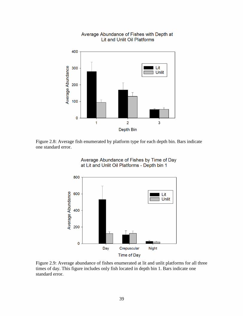
Average fish counts were highest in depth bin 1 for lit platforms and depth bin 2

for unlit platforms. Average counts at depth bin 3 were nearly identical (Figure 2.8). The

number of fishes enumerated was highest at lit platforms during the day, with average

values more than four times the next closest average abundance value (Figure 2.9).

Counts were nearly identical between lit and unlit platforms at night and during

crepuscular periods (Figure 2.9).

39

Figure 2.8: Average fish enumerated by platform type for each depth bin. Bars indicate one standard error.

Figure 2.9: Average abundance of fishes enumerated at lit and unlit platforms for all three times of day. This figure includes only fish located in depth bin 1. Bars indicate one standard error.

40

DISCUSSION

Oil and gas platforms have been shown to increase hard substrate in the GOM and

provide artificial reef habitat for reef-associated and migratory fish species (Stanley and

Wilson 1991, 1997, Wilson et al. 2003, Keenan et al. 2007, Szedlmayer 2007). However,

the impact of artificial night lighting has never been examined as a potential driver of fish

community differences. The goal of this study was to determine potential differences in

fish community structure surrounding lit and unlit oil and gas platforms in the northern

GOM, focusing on variables such as depth, platform type, and season.

Diversity indices including species richness (S), Shannon Diversity (H’), and

Pielou’s Evenness (J’) showed no significant difference existed between platform types

for any of the three metrics. This is likely because the platforms are in close proximity (<

10 km apart) and therefore the same fish species inhabit the waters surrounding both lit

and unlit structures. Species richness was significantly different between seasons and

among times of day. The results mirror those in Stanley and Wilson (2000b, 2003) who

reported that fish community structure around oil platforms was highly variable,

changing with depth, distance from platform, time of day, and season. Species richness

was similar to previous studies conducted on oil platforms (Langland 2015, Reynolds

2015), though much lower than values from natural reefs (Rooker et al. 1997, Langland

2015). Multiple studies (Carr and Hixon 1997, Schroeder et al. 2000, Wells et al. 2007)

have shown that species richness is greater on natural reefs than artificial reefs, likely due

to a lack of fouling community growth on platform legs, which provides cover for small

fish to avoid predators. The relatively low species richness values observed during this

study support these results.

41

The results highlight the highly variable nature of fish community structure

around artificial reefs in the GOM. Spatial and temporal variability was observed with

platform type, depth, and season. Lit platforms provided habitat for more fishes than unlit

platforms and the effect of platform lighting was evident when examining average fish

abundance in the upper water column. While more fish were enumerated in the top 30 m

than any other depth bin, it was only during the day. At night, fish avoided the surface

waters at both lit and unlit platforms, likely in response to enhanced predation pressure.

Under typical conditions, zooplankton and fish exhibit a diel vertical migration, in

which plankton stay at depth during the day and come to the surface at night to feed.

Planktivorous fishes come to the surface waters to feed on the abundance of zooplankton,

which in turn attracts predatory fish species (see Brierley 2014 for review). However, it is

possible that typical fish stratifications can change under varying light regimes. Fish have

been shown to alter their behavior in response to bright moonlight (Luecke and

Wurtsbaugh 1993) and artificial night lighting (Blaxter 1980, Batty et al. 1990, Ryer and

Olla 1998, 1999). As artificial light increases, fish have been shown to establish nocturnal

schools in an effort to reduce predation risk (Nightingale et al. 2005). The late night

“antipredator window” of relative safety is often either reduced or even eliminated as

surface lighting aids predators in identifying prey from below. Further, Simonson (2013)

noticed a complete breakdown of the typical diel migrations at lit platforms in the GOM.

She found that fish were remaining at depth at night, which suggests that the risk of

nocturnal predation overwhelms the desire for easy foraging at the surface. While the

results in Simonsen have not yet been published, my results are consistent with this

premise.

42

The distLM model indicated that temperature strongly influenced the fish

community composition. This is likely due to the wide range of temperature extremes at

the surface, while temperatures at deeper depth remained relatively constant. For

example, temperature at 80 m deep ranged from 19.5 – 22 °C, whereas at 10 m deep, the

temperature shifted by as much as 10 °C from summer to winter. Many studies (Sonnier

et al. 1976, Rooker et al. 1997, Stanley and Wilson 2000a, Allen et al. 2006) have shown

that fish communities vary with depth, and that snapper and grouper species comprise the

majority of individuals near the sea floor, resulting in a more stable community structure

at depth. Meanwhile, small schooling fishes tend to occupy the surface waters, perhaps

migrating with temperature and food availability. This may result in a more variable

community structure at the surface.

Blue runner (Caranx crysos) were numerically dominant during all season by

type, season by depth, and season by time of day interactions. This result is in contrast to

Reynolds (2015), who found red snapper (Lutjanus campechanus) to be numerically

dominant. The results of this study are more similar to Stanley and Wilson (2003), which

found that blue runner were the dominant species around GOM platforms, comprising

20.6% of the fish abundance, followed by red snapper (10.8%). Blue runner are a

surface-oriented, schooling species that is commonly found around oil and gas platforms

in the GOM (Sonnier et al. 1976, Rooker et al. 1997, Stanley and Wilson 2000a, 2003,

Hernandez et al. 2003), but also in the open GOM away from structured habitat. Due to

their schooling behavior, it was not uncommon to see 200+ runners in a single frame.

Further, schooling served as anti-predator behavior, which caused blue runners to

approach the camera at all times of day, while individual fish hid in the platform at night.

43

BRUVs allowed for accurate, standardized sampling at deep-water oil platforms

that would be inaccessible to divers. While baited systems serve as an attractant for many

predatory species of fish, they have been shown to potentially underestimate the

abundance of herbivorous species, resulting in bias (Watson et al. 2005, Harvey et al.

2007, Watson et al. 2010). However, consistent sampling methodology and post-

processing techniques served to minimize these effects. Additionally, a large sample size

(62 surveys with three depths sampled per drop) helped to reduce potential sources of

error that are inherent in small sample size surveys.

This study is the first to directly examine the impact of artificial night lighting on

fish community structure around oil and gas platforms in the GOM. Further research in

this area would be helpful to determine if the trends observed in this study continue over

time. Due to sampling limitations, only 11 drops were conducted at night and only took

place during the summer and fall seasons. For a more complete survey, nocturnal surveys

spanning the course of a full year would be beneficial to determining nocturnal changes

in community composition over time. Further, drops were only conducted on one side of

the platform, down current of the platform. This resulted in an incomplete view of the

fish community structure. As the biological effects of oceanographic parameters can be

sporadic over time, further attempts to study nocturnal fish community biomass would

benefit from more regular, long-term sampling across a variety of water depths and

platform sizes.

44

LITERATURE CITED

Allen, Y., K. Boswell, M. Miller, D. Nieland, and C. Wilson. 2006. Effects of depth, location, and habitat type on relative abundance and species composition of fishes associated with petroleum platforms and Sonnier Bank in the northern Gulf of Mexico. M. M. S. U.S. Dept. of the Interior, Gulf of Mexico OCS Region. New Orleans, LA. 85 pages.

Batty, R. S., J. Blaxter, and J. M. Richard. 1990. Light intensity and the feeding

behaviour of herring, Clupea harengus. Marine Biology 107:383-388. Blaxter, J. H. S. 1980. Vision and feeding of fishes. Pages 32-56 in J.E. Bardach, J.J.

Magnuson, R.C. May, and J.M. Reinhart, editors. Fish behavior and its use in the capture and culture of fishes. ICLARM Conference Proceedings 5, International Center for Living Aquatic Resources Management, Manila, Philippines.

Boswell, K. M., R. J. D. Wells, J. H. Cowan, Jr., and C. A. Wilson. 2010. Biomass,


Brierley, A. S. 2014. Diel vertical migration. Current Biology 24:R1074-R1076.

Bureau of Safety and Environmental Enforcement (BSEE). 2015. Platform/Rig

Information.http://www.data.bsee.gov/homepg/data_center/platform/platform.asp. Last accessed June 10, 2015.

Cappo, M., E. S. Harvey, H. Malcolm, and P. Speare. 1999. Potential of video

techniques to monitor diversity, abundance, and size of fish in studies of marine protected areas. Pages 455-464 in Aquatic Protected Areas - what works best and how do we know.

Cappo, M., E. Harvey, and M. Shortis. 2006. Counting and measuring fish with baited

video techniques-an overview. Pages 101–114 in Lyle, J.M., Furlani D.M., Buxton C.D., editors. Cutting-edge technologies in fish and fisheries science. Australian Society for Fish Biology Workshop. Australian Society of Fish Biology, Hobart.

Carr, M. H., and M. A. Hixon. 1997. Artificial reefs: the importance of comparisons

with natural reefs. Fisheries 22:28-33.

Dugas, R., V. Guillory, and M. Fischer. 1979. Oil rigs and offshore sport fishing in Louisiana. Fisheries 4:2-10.

Franks, J. S. 2000. Pelagic fishes at petroleum platforms in the Northern Gulf of

Mexico; diversity, interrelationships, and perspective in Pêche thonière et dispositifs de concentration de poissons, Caribbean-Martinique, 15-19 Oct 1999.

45

Froese, R. and D. Pauly. 2014. FishBase. http://www.fishbase.us/search.php. Last

accessed June 10, 2015. Harvey, E. S., M. Cappo, J. J. Butler, N. Hall, and G. A. Kendrick. 2007. Bait attraction

affects the performance of remote underwater video stations in assessment of demersal fish community structure. Marine Ecology Progress Series 350:245-254.

Harvey, E. S., D. Fletcher, and M. Shortis. 2002. Estimation of reef fish length by

divers and by stereo-video: a first comparison of the accuracy and precision in the field on living fish under operational conditions. Fisheries Research 57:255-265.

Hiett, R. L., and J. W. Milon. 2002. Economic Impact of Recreational Fishing and

Diving Associated with Offshore Oil and Gas Structures in the Gulf of Mexico. Food and Agriculture Organization of the United Nations.

Keenan, S. F., M. C. Benfield, and J. K. Blackburn. 2007. Importance of the artificial


Hernandez, F. J., Jr., R. F. Shaw, J. S. Cope, J. G. Ditty, T. Farooqi, and M. C.

Benfield. 2003. The across-shelf larval, postlarval, and juvenile fish assemblages collected at offshore oil and gas platforms west of the Mississippi River delta. Pages 39-72 in D.R. Stanley and A. Scarborough-Bull, editors. Fisheries, reefs, and offshore development. American Fisheries Society, Symposium 36, Bethesda, Maryland.

Langland, T. 2015. Fish asssemblage structure, distribution, and trophic ecology at

northwestern Gulf of Mexico banks. Ph.D. dissertation. Louisiana State University, Baton Rouge.

Luecke, C., and W. A. Wurtsbaugh. 1993. Effects of moon and daylight on

hydroacoustic estimates of pelagic fish abundance. Transactions of the American Fisheries Society 122:112–120.

Nightingale, B., T. Longcore, and C. A. Simenstad. 2005. Artificial night lighting and

fishes. Pages 257-276 in T. Longcore and C. Rich, editors. Ecological Consequences of Artificial Night Lighting. Island Press, Washington.

Priede, I., P. Bagley, A. Smith, S. Creasey, and N. Merrett. 1994. Scavenging deep

demersal fishes of the Porcupine Seabight, North-east Atlantic: observations by baited camera, trap and trawl. Journal of the Marine Biological Association of the United Kingdom 74:481-498.

46

Reynolds, E. 2015. Fish biomass and community structure around standing and toppled oil and gas platforms in the northern Gulf of Mexico using hydroacoustic and video surveys. M.S. Thesis. Louisiana State University, Baton Rouge.



Ryer, C. H., and B. L. Olla. 1998. Effect of light on juvenile walleye pollock shoaling

and their interaction with predators. Marine Ecology Progress Series 167:215-226.

Ryer, C. H., and B. L. Olla. 1999. Light-induced changes in the prey consumption and

behavior of two juvenile planktivorous fish. Marine Ecology Progress Series 181:41-51.

Scarborough Bull, A., and J. J. Kendall, Jr. 1994. An indication of the process: offshore

platforms as artificial reefs in the Gulf of Mexico. Bulletin of Marine Science 55:1086-1098.

Schroeder, D. M., A. J. Ammann, J. A. Harding, L. A. MacDonald, and W. T. Golden.

2000. Relative habitat value of oil and gas production platforms and natural reefs to shallow water fish assemblages in the Santa Maria Basin and Santa Barbara Channel, California. Pages 493-498 in Proc. Fifth California Islands Symposium.

Simonsen, K. A. 2013. Reef fish demographics on Louisiana artificial reefs: the effects

of reef size on biomass distribution and foraging dynamics. Ph.D. dissertation. Louisiana State University, Baton Rouge.

Sonnier, F., J. Teerling, and H. Dickson Hoese. 1976. Observation on the offshore reef

and platform fish fauna of Louisiana. Copeia 1976:105-111. Stanley, D. R., and C. A. Wilson. 1991. Factors affecting the abundance of selected

fishes near oil and gas platforms in the northern Gulf of Mexico. Fishery Bulletin 89:149-159.

Stanley, D. R., and C. A. Wilson. 1996. Abundance of fishes associated with a

petroleum platform as measured with dual-beam hydroacoustics. ICES Journal of Marine Science: Journal du Conseil 53:473-475.



47

Stanley, D. R., and C. A. Wilson. 2000a. Variation in the density and species composition of fishes associated with three petroleum platforms using dual beam hydroacoustics. Fisheries Research 47:161-172.

Stanley, D. R., and C. A. Wilson. 2000b. Seasonal and spatial variation in the biomass

and size frequency distribution of fish associated with oil and gas platforms in the northern Gulf of Mexico. OCS Study MMS 2000-005:252.

Stanley, D. R., and C. A. Wilson. 2003. Seasonal and spatial variation in the biomass

and size frequency distribution of fish associated with oil and gas platforms in the northern Gulf Of Mexico. Pages 125-153 in Stanley, D.R. and A. Scarborough-Bull, editors. Fisheries, Reefs, and Offshore Development. American Fisheries Society, Symposium 36, Bethesda, Maryland.

Stobart, B., J. A. García-Charton, C. Espejo, E. Rochel, R. Goñi, O. Reñones, A.

Herrero, R. Crec'hriou, S. Polti, C. Marcos, S. Planes, and A. Pérez-Ruzafa. 2007. A baited underwater video technique to assess shallow-water Mediterranean fish assemblages: Methodological evaluation. Journal of Experimental Marine Biology and Ecology 345:158-174.

Szedlmayer, S. 2007. An evaluation of the benefits of artificial habitats for red snapper,

Lutjanus campechanus, in the northeast Gulf of Mexico. Proceedings of the Gulf and Caribbean Fisheries Institute, 59:223-230.

Watson, D. L., E. S. Harvey, M. J. Anderson, and G. A. Kendrick. 2005. A comparison

of temperate reef fish assemblages recorded by three underwater stereo-video techniques. Marine Biology 148:415-425.

Wells, R. D., J. H. Cowan, Jr. 2007. Video estimates of red snapper and associated fish

assemblages on sand, shell, and natural reef habitats in the north-central Gulf of Mexico. Pages 39-58 in W. F. Patterson, III, J. H. Cowan, Jr., G. R. Fitzhugh, and D. L. Nieland, editors. Red snapper ecology and fisheries in the U.S. Gulf of Mexico. American Fisheries Society, Symposium 60, Bethesda, MD.

Wilson, C. A., A. Pierce, and M. W. Miller. 2003. Rigs and Reefs: a comparison of the

fish communities at two artificial reefs, a production platform, and a natural reef in the northern Gulf of Mexico. Mineral Management Service, OCS Study MMS 2003- 009, New Orleans, 95 p.

48

CHAPTER 3: SPATIAL AND TEMPORAL DISTRIBUTION OF REEF-ASSOCIATED FISHES AROUND ACTIVE AND

DECOMMISSIONED OIL AND GAS PLATFORMS IN THE NORTHERN GULF OF MEXICO

INTRODUCTION

Nearly 6,000 oil and gas platforms were placed in the Gulf of Mexico (GOM)

since the 1940’s, inadvertently creating the largest artificial reef complex in the world

(Dauterive 2000). Sampling fishes at these structures can be difficult, due to their

immense size and distance from shore (LARP 2015). However, the abundance and

community composition of fishes using these structures must be quantified, and the

biological significance of platforms fully understood. Both stationary and mobile

hydroacoustic (acoustic) surveys have proven to be useful in describing the spatial and

temporal distribution of fishes around these platforms.

“Echosounding” technology, and the hydroacoustic data it produces, have existed

since the 1920’s when sonar was utilized to detect submarines during wartime

(Simmonds and MacLennan 2005). Hydroacoustic data can also provide valuable

estimates of fish acoustic biomass, density, spatial distribution, and area of influence

around artificial structures. Hydroacoustics are not limited by poor visibility and has

minimal impact on fish behavior, resulting in a “snapshot” of fish acoustic biomass.

Additionally, using mobile hydroacoustics allows researchers to sample a large area

quickly. However, due to the low resolution of hydroacoustic data, having mostly to do

with high species diversity and little information on target strength by species, it is often

used in conjunction with other survey methods, such as stereo-video cameras or trawling.

49

This makes it possible determine not only biomass around the platform, but also which

species are present and their relative abundances.

Today, hydroacoustic systems consist of at least one transducer that produces

pulses of sound, or pings, that are transmitted into the surrounding water. Transducers are

available in single-, dual-, and split-beam varieties and generally have a range of 1500 –

2000 meters, making them suited for all but the deepest oceanic research (Kalikhman and

Yudanov 2006). They can be either mounted on a stationary object such as the platform

itself (Stanley and Wilson 1996, 1997, 2000) or be towed around structures off the side of

a research vessel (Boswell et al. 2010, Simonsen 2013, Harwell 2013, Reynolds 2015),

making hydroacoustics a versatile fisheries-independent monitoring tool.

The sound energy produced by the transducer is scattered when it encounters

objects of different density than the surrounding medium, such as suspended particles,

organisms, or entrained gas, and is deflected outwards in all directions (Simmonds and

MacLennan 2005). This reflected energy, averaged over a given volume, is the mean

volume backscatter (MVBS; Sv), which is a known proxy for biomass. MVBS is

measured in decibels on a log scale and this value is always negative (Simmonds and

MacLennan 2005).

Backscatter values are impacted by both the size of an isonified object and the

density difference recorded. According to Rayleigh’s Law, doubling the size of the

isonified object intensifies the amount of scattering 64 fold (Kalikhman and Yudanov

2006). In addition to increasing size, the greater the difference in density between the

object detected and the surrounding water, the greater the backscatter; therefore, large

pockets of trapped air, such as in a fish’s swimbladder, produce larger MVBS values. The

50

swimbladder is responsible for up to 90% of a teleost fish’s acoustic echo (Foote 1980).

The backscatter is then converted into a diagram of the water column, called an

echogram, which can be analyzed by researchers to determine proxies for biomass,

density, and schooling behavior.

Many studies have been conducted to examine the spatial distribution of fishes

around artificial reef structures around the world (Fabi and Sala 2002, Boswell et al.

2010, Harwell 2013, Simonsen 2013, Reynolds 2015). It has been shown that fish

concentrate inside and around the platforms, with biomass and abundance dropping off

with increasing distance from the structure. The size of this “area of influence” is likely

dependent upon local conditions but has been found to extend up to 100 m from oil

platforms, depending upon the sampling technique used (Soldal et al. 2002, Simonsen

2013). Most studies cite this area of high fish abundance as within 20 – 100 meters of the

structure, depending upon reef size (Stanley and Wilson 1996, 1997, 2000, Fabi and Sala

2002, Boswell et al. 2010).

The goal of this study was to quantify nektonic MVBS around two lit and three

unlit oil and gas platforms in relation to type of platform, season, depth, distance away

from the structure, and time of day. The working hypotheses were that 1) MVBS

(hereafter acoustic biomass) would be greater at lit versus unlit platforms, and 2) acoustic

biomass would be concentrated around the platform and decrease with increasing

distance.

51

METHODS AND MATERIALS

Study Sites

Five oil and gas platforms located approximately 130 km off the coast of

Louisiana in the Eugene Island Oil and Gas Lease Planning Area were selected for this

study. Two operational lit oil and gas platforms (hereafter lit) and three decommissioned

unlit oil and gas platforms (hereafter unlit) were examined. Lit platforms are lighted

using high-pressure mercury vapor floodlights around the exterior of the structure,

allowing for normal working operations to proceed 24 hours a day. An additional source

of illumination is a natural gas flare stack, which periodically combusts any natural gas or

petroleum byproducts released (Keenan et al. 2007). Unlit platforms are only minimally

lit for the purpose of avoidance by vessel traffic. All platforms are located on the

continental shelf in water depths of approximately 75-90 m (Figure 3.1) (Table 3.1).

Figure 3.1: Study sites located in the Eugene Island Oil and Gas Planning Area. Inactive platforms include EI303A, EI325A, and EI320B. Active platforms include EI342C and EI346A.

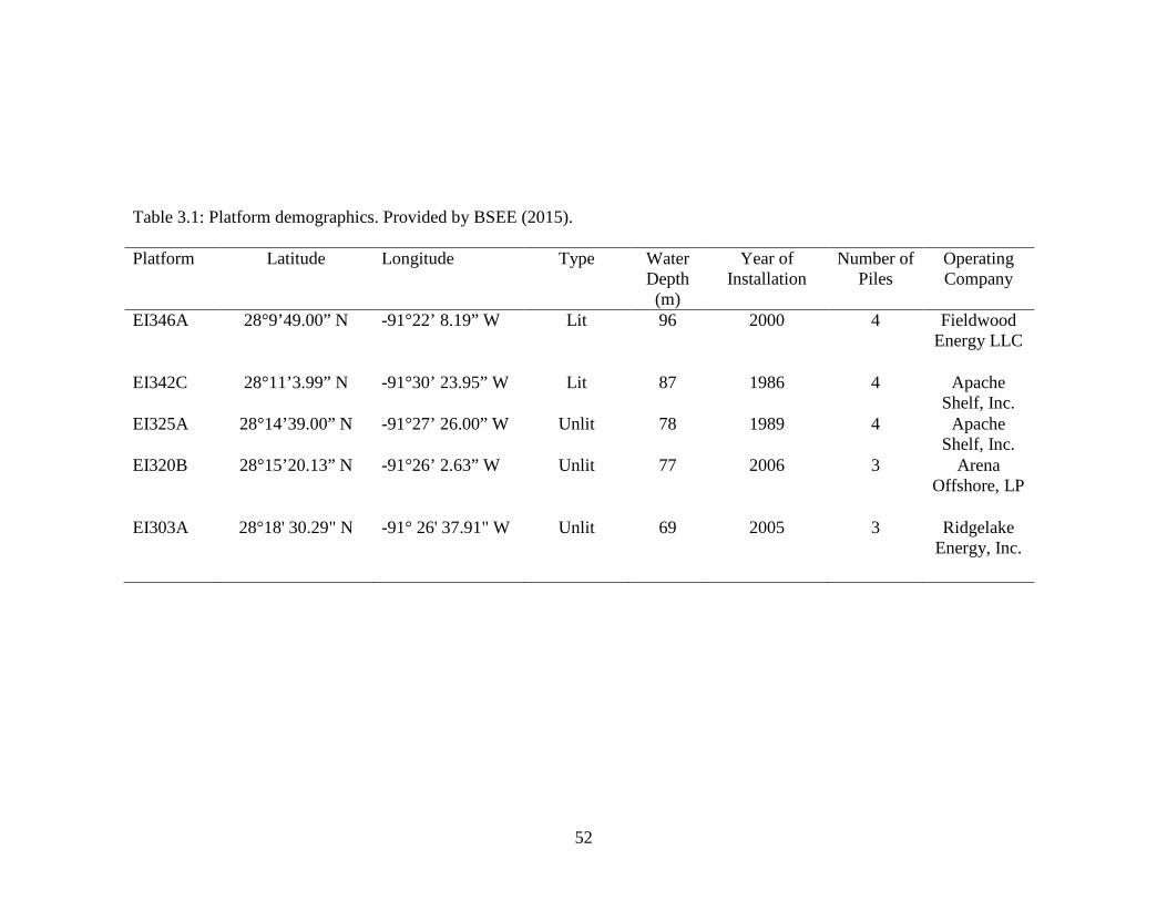
52

Table 3.1: Platform demographics. Provided by BSEE (2015).

Platform Latitude Longitude Type Water Depth (m)

Year of Installation

Number of Piles

Operating Company

EI346A 28°9’49.00” N -91°22’ 8.19” W Lit 96 2000 4 Fieldwood Energy LLC

EI342C 28°11’3.99” N -91°30’ 23.95” W Lit 87 1986 4 Apache Shelf, Inc.

EI325A 28°14’39.00” N -91°27’ 26.00” W Unlit 78 1989 4 Apache Shelf, Inc.

EI320B 28°15’20.13” N -91°26’ 2.63” W Unlit 77 2006 3 Arena Offshore, LP

EI303A 28°18' 30.29" N -91° 26' 37.91" W Unlit 69 2005 3 Ridgelake Energy, Inc.

53

Sampling Procedure

Acoustic surveys were conducted quarterly from February 2014 through

November 2015, as weather and scheduling permitted. Due to unforeseen circumstances

related to vessel availability, no sites were sampled between June and December 2014.

Acoustic transects were conducted opportunistically during both day and night to

examine diel changes in acoustic biomass and spatial distribution. Environmental data

were collected at each site during each sampling trip with a Sea-Bird SBE 25

conductivity, temperature, and depth (CTD) profiler. The CTD was acclimated to the

saltwater for approximately three minutes at the surface and then deployed vertically at a

rate of approximately 1 m/s. Water quality parameters recorded included conductivity,

temperature, depth, salinity, and dissolved oxygen. Temperature and salinity values were

necessary to calibrate the sound speed correction during analysis. Environmental data

were post-processed with Visual Acquisition v. 6 software (BioSonics, Seattle, WA,

USA).

Acoustic backscatter data were collected with a BioSonics echosounder equipped

with three downward-facing split-beam transducers (70, 123, and 206 kHz). However,

only data from the 70 kHz transducer were used in this analysis, as this frequency most

accurately detects fish with swimbladders (Kalikhman and Yudanov 2006). Transducers

were mounted on a pivoting boom that extends approximately 2 m below the sea surface

to avoid noise from the vessel’s wake. Data were collected with a pulse duration of 0.4

ms. Surveys were conducted at an average speed of 5.5 knots and took approximately 1.5

hours to complete. Ten transects, each 0.5 km long, were completed at each site and

conducted in a rosette pattern with the structure in the geographic center of the survey.

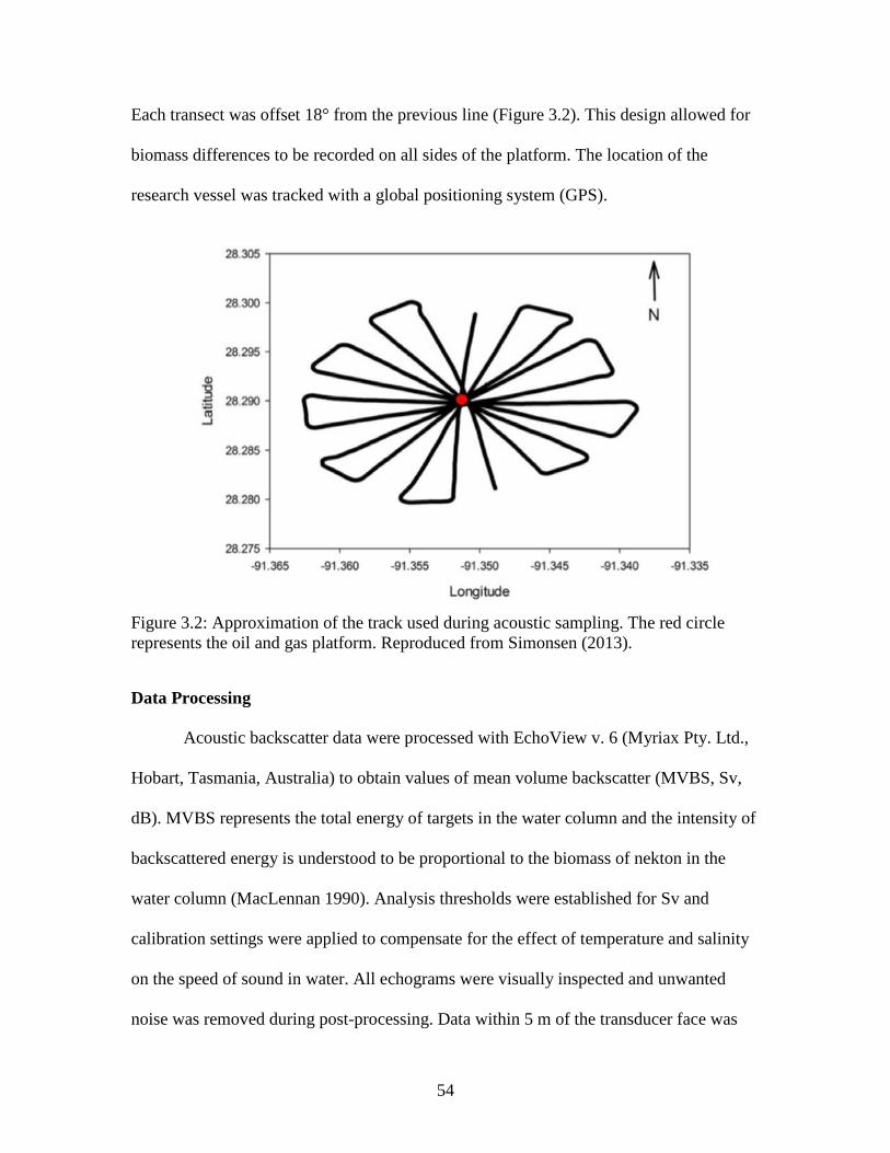
54

Each transect was offset 18° from the previous line (Figure 3.2). This design allowed for

biomass differences to be recorded on all sides of the platform. The location of the

research vessel was tracked with a global positioning system (GPS).

Figure 3.2: Approximation of the track used during acoustic sampling. The red circle represents the oil and gas platform. Reproduced from Simonsen (2013).

Data Processing Acoustic backscatter data were processed with EchoView v. 6 (Myriax Pty. Ltd.,

Hobart, Tasmania, Australia) to obtain values of mean volume backscatter (MVBS, Sv,

dB). MVBS represents the total energy of targets in the water column and the intensity of

backscattered energy is understood to be proportional to the biomass of nekton in the

water column (MacLennan 1990). Analysis thresholds were established for Sv and

calibration settings were applied to compensate for the effect of temperature and salinity

on the speed of sound in water. All echograms were visually inspected and unwanted

noise was removed during post-processing. Data within 5 m of the transducer face was

55

excluded to account for near field effects and transducer ring down. A bottom detection

algorithm (best bottom candidate) was applied to exclude data within 1 m of the seafloor

and was manually edited as needed to remove unwanted backscatter (i.e. artificial

material, platform debris, gas seeps). Background noise was removed following the

methods of De Robertis and Higginbottom (2007). Sporadic noise spikes were suppressed

with an algorithm following Anderson et al. (2005) (Figure 3.3). A grid was applied to

the echogram in 10 m depth by 20 m distance bins, yielding information on spatial

acoustic biomass changes both horizontally and vertically around the structure.

Data from the 70 kHz transducer were exported from EchoView after the volume

backscatter coefficient (sv) was integrated over each cell (10 m x 20 m) to acquire MVBS

using the relationship:

Sv=10log10(sv)

where Sv is the mean volume backscatter (dB) and sv is the volume backscattering

coefficient (m-1). sv is represented by the equation:

sv = Σσbs/V

where V is the volume occupied by the scattering medium or multiple discrete targets and

σbs is the variance of the backscattering cross-section represented by the equation:

σbs = [r2Ibs(r)10ar/10 / Iinc]

where r is the distance of measurement position from a small target, Ibs(r) is the intensity of the backscattered wave, a is the area of a school observed in the echogram, and Iinc is the intensity of the transmitted wave at the target (Maclennan et al. 2002, Simmonds and MacLennan 2005).

56

Figure 3.3: Schematic of the flow of data in EchoView® that was used to remove spike noise when present, adapted from Anderson et al. (2005). Sv: volume backscattering strength.

57

Data Analysis The distribution of MVBS was compared across type of platform, depth, season,

time of day, and distance from structure. The geographic center point for each platform

was determined from BSEE (2015) and distance bins based upon that point were created

in SAS v 9.4 (Cary, North Carolina, USA). Both Simonsen (2013) and Reynolds (2015)

conducted acoustic surveys at several of the same platforms surveyed in this study and

saw a clear decrease of acoustic biomass with distance away from the platform, with

MVBS concentrated within 100 m of the structure. Due to these findings, transects in this

study were constrained to only 100 m around the platforms. The distance bins established

were 0 – 10 m, 11 – 20 m, 21 – 30 m, 31 – 40 m, 41 – 50 m, 51 – 60 m, 61 – 70 m, 71 –

80 m, 81 – 90 m, and 91 – 100 m, referred to as bins 1 – 10, respectively. Due to limited

data closely adjacent to the platform, distance bin 1 was removed from the SAS mixed

model analysis. Depth layers were created by dividing the water column into thirds: 0 –

30 m, 30 – 60 m, and >60 m, referred to as depths 1, 2, and 3, respectively. Seasons were

defined as summer (June, July, August), fall (September, October, November), winter

(December, January, February), and spring (March, April, May). Types were defined as

either lit or unlit, with replicates in each group. Time of day was defined as either day

(06:00 – 20:00) or night (20:00 – 06:00).

The spatial distribution of MVBS around lit and unlit platforms was examined

with a generalized linear mixed model (GLIMMIX) in SAS, with MVBS as the

dependent variable. The full model included season, time of day, type, depth bin, and

horizontal bin. As all variables were significant as second-order interactions, no variables

were removed from the model. The residuals were examined for normality with a

58

Kolmogorov–Smirnov test. A Tukey post-hoc test was conducted to test for pairwise

comparisons. CTD data (temperature, salinity, dissolved oxygen) were plotted as the

mean ± standard error (X ± SE) at discrete depths (every 10 meters for the top 100

meters) to examine differences in environmental data across season and water depth.

Traditional statistical models such as GLIMMIX often have difficulty analyzing

data with a large number of degrees of freedom, such as in this study. To avoid this

problem, the acoustic data were also analyzed with regression trees, which are able to

model complex, non-linear relationships between fishes and their environment. They are

able to draw interpretable results where traditional statistical methods such as parametric

models are unsuited (De'ath and Fabricius 2000). Regression trees use recursive binary

partitioning to determine which variables explain the greatest amount of variability

observed in the data. The regression tree bases its selection on the variable with the

smallest sum of squares of the error, or SSE. After the variable has been selected, the tree

‘splits’ into two mutually exclusive groups, with biomass values in either ‘branch’ as

homogenous as possible (De'ath and Fabricius 2000). Factors tested included depth (m),

distance from platform (m), time of day, temperature (°C), salinity (PSU), dissolved

oxygen (mg/L), site, platform surface area (m2), and type of platform (lit/unlit).

Regression trees were run for day only transects, night only transects, and all transects

combined to evaluate time of day effects. All regression trees were calculated in R

Statistical Package ‘tree’ (Ripley 2015). Trees were pruned to aid data interpretation.

59

RESULTS

A total of 47 hydroacoustic surveys were conducted between February 2014 and

November 2015. Data collected during the day accounted for 53.50% of all data collected

while 46.50% of the data points were collected at night. This provided a representative

sample of both day and nocturnal biomass. In total, 26,284 data points between 0 and 100

m from the platform were collected. Data were not split evenly between sites with

13.25% from EI303A, 29.47% from EI320B, 12.91% from EI325A, 16.65% from

EI342C, and 27.71% from EI346A. This is due to the late addition of EI303A after

EI325A was removed in June 2015. Unlit platforms accounted for 55.63% of the cells

analyzed while lit platforms accounted for 44.37%. Data were not evenly distributed

among seasons, due to weather-limited sampling in the spring months, with 8.04% of

data collected in spring, 36.98% in summer, 26.15% in fall, and 28.82% in winter.

The CTD profiles indicated a stratified water column with a strong thermocline

and halocline during the summer. During winter months, the water column was well

mixed. Temperature (°C), salinity (PSU), and dissolved oxygen (mg/L) showed similar

patterns at both lit and unlit platforms (Figures 3.4, 3.5, and 3.6, respectively).

Mixed Model

The MVBS mixed model indicated that time of day, depth, and distance were

significant as well as were all of the second order interactions (p < 0.0001, Table 3.2).

For both platform types, MVBS was highest directly adjacent to the geographic center

point of the platform and declined with distance. While the type was not significant as a

main effect, it was significant in two-way interactions.

60

Figure 3.4: Temperature (°C) for both lit and unlit platforms. Error bars indicate one standard error.

61

Figure 3.5: Oxygen (mg/L) for both lit and unlit platforms. Error bars indicate one standard error.

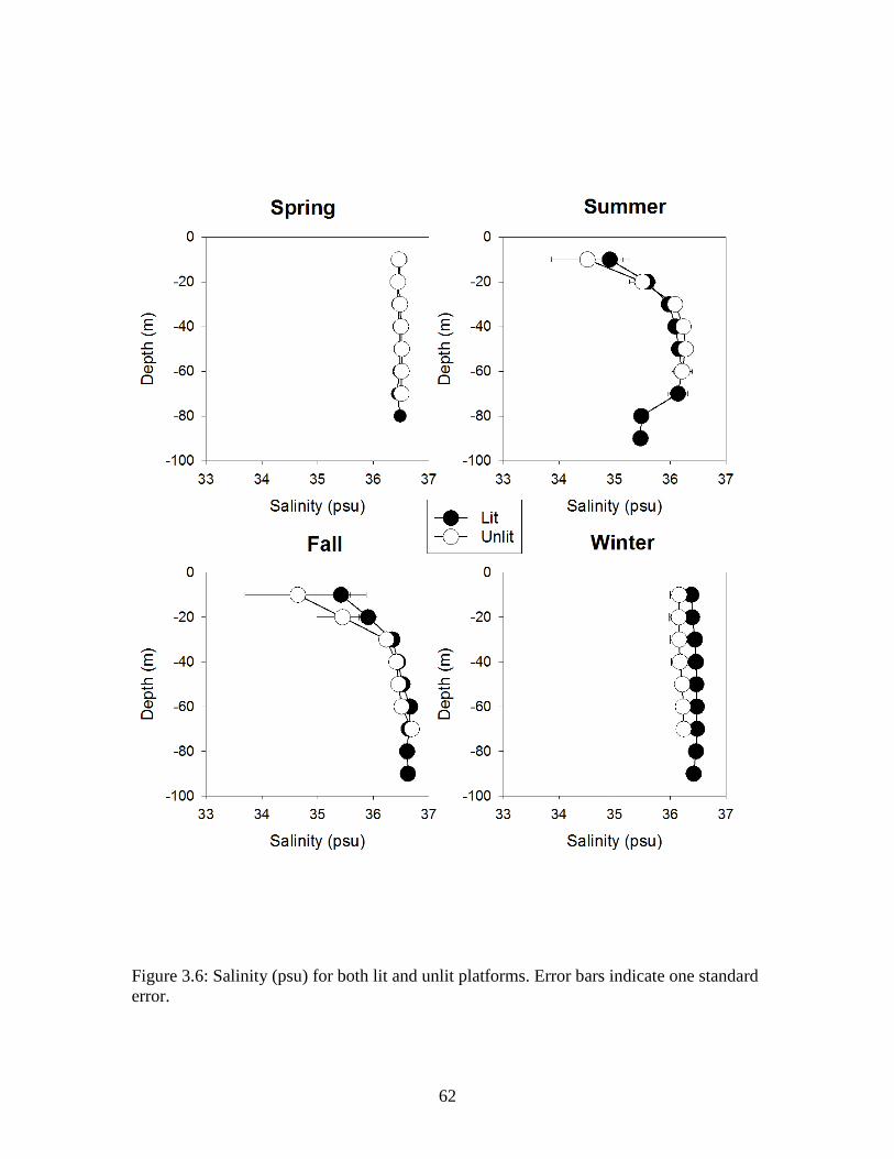
62

Figure 3.6: Salinity (psu) for both lit and unlit platforms. Error bars indicate one standard error.

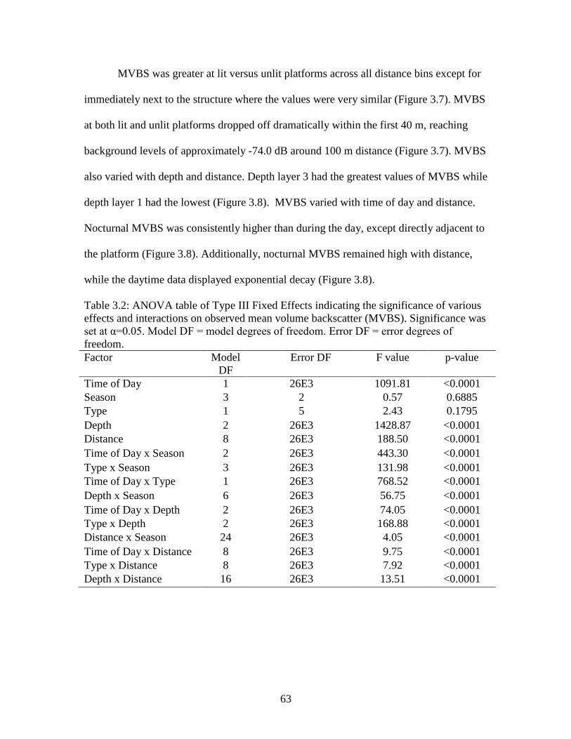
63

MVBS was greater at lit versus unlit platforms across all distance bins except for

immediately next to the structure where the values were very similar (Figure 3.7). MVBS

at both lit and unlit platforms dropped off dramatically within the first 40 m, reaching

background levels of approximately -74.0 dB around 100 m distance (Figure 3.7). MVBS

also varied with depth and distance. Depth layer 3 had the greatest values of MVBS while

depth layer 1 had the lowest (Figure 3.8). MVBS varied with time of day and distance.

Nocturnal MVBS was consistently higher than during the day, except directly adjacent to

the platform (Figure 3.8). Additionally, nocturnal MVBS remained high with distance,

while the daytime data displayed exponential decay (Figure 3.8).

Table 3.2: ANOVA table of Type III Fixed Effects indicating the significance of various effects and interactions on observed mean volume backscatter (MVBS). Significance was set at α=0.05. Model DF = model degrees of freedom. Error DF = error degrees of freedom. Factor Model

DF Error DF F value p-value

Time of Day 1 26E3 1091.81 <0.0001 Season 3 2 0.57 0.6885 Type 1 5 2.43 0.1795 Depth 2 26E3 1428.87 <0.0001 Distance 8 26E3 188.50 <0.0001 Time of Day x Season 2 26E3 443.30 <0.0001 Type x Season 3 26E3 131.98 <0.0001 Time of Day x Type 1 26E3 768.52 <0.0001 Depth x Season 6 26E3 56.75 <0.0001 Time of Day x Depth 2 26E3 74.05 <0.0001 Type x Depth 2 26E3 168.88 <0.0001 Distance x Season 24 26E3 4.05 <0.0001 Time of Day x Distance 8 26E3 9.75 <0.0001 Type x Distance 8 26E3 7.92 <0.0001 Depth x Distance 16 26E3 13.51 <0.0001

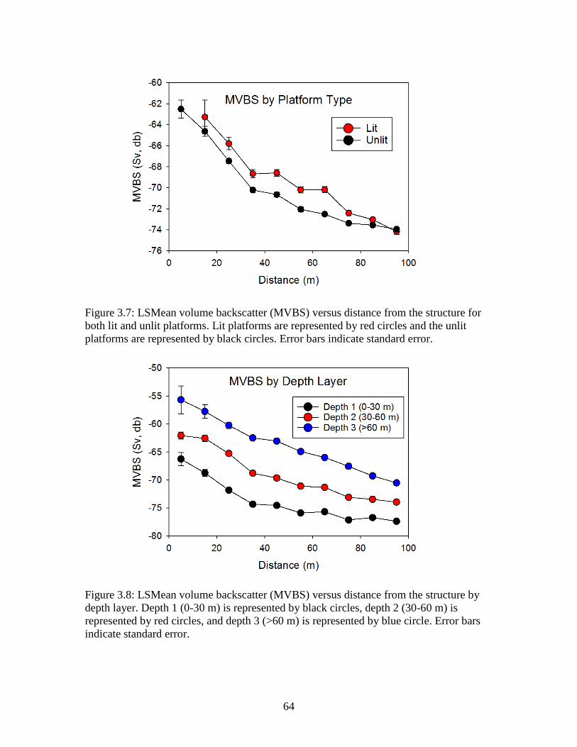
64

Figure 3.7: LSMean volume backscatter (MVBS) versus distance from the structure for both lit and unlit platforms. Lit platforms are represented by red circles and the unlit platforms are represented by black circles. Error bars indicate standard error.

Figure 3.8: LSMean volume backscatter (MVBS) versus distance from the structure by depth layer. Depth 1 (0-30 m) is represented by black circles, depth 2 (30-60 m) is represented by red circles, and depth 3 (>60 m) is represented by blue circle. Error bars indicate standard error.

65

Figure 3.9: LSMean volume backscatter (MVBS) versus distance from the structure for time of day. Night data are represented by red circles; day data are represented by black circles. Error bars indicate standard error.

Regression Tree

All data Only four of the eight variables included in the model were chosen by the

software to create any of the three regression trees: depth (m), distance from platform

(m), temperature (°C), and oxygen (mg/L). The regression tree indicated that depth was

the most important variable in determining MVBS, splitting MVBS values at 15.0 meters

(Figure 3.10). Depths shallower than 15.0 m were influenced by environmental factors,

splitting again on both temperature and dissolved oxygen (Figure 3.10). The MVBS

values at depths greater than 15.0 m split again into depths between 15.0 – 73.2 m and

depths >73.2 m. The middle depth (15.0 m – 73.2 m) further divided with distance away

from platform (45.8 m). The deepest depths split at 66.1 m away from the platform, with

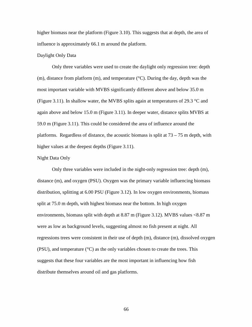
66

higher biomass near the platform (Figure 3.10). This suggests that at depth, the area of

influence is approximately 66.1 m around the platform.

Daylight Only Data

Only three variables were used to create the daylight only regression tree: depth

(m), distance from platform (m), and temperature (°C). During the day, depth was the

most important variable with MVBS significantly different above and below 35.0 m

(Figure 3.11). In shallow water, the MVBS splits again at temperatures of 29.3 °C and

again above and below 15.0 m (Figure 3.11). In deeper water, distance splits MVBS at

59.0 m (Figure 3.11). This could be considered the area of influence around the

platforms. Regardless of distance, the acoustic biomass is split at 73 – 75 m depth, with

higher values at the deepest depths (Figure 3.11).

Night Data Only

Only three variables were included in the night-only regression tree: depth (m),

distance (m), and oxygen (PSU). Oxygen was the primary variable influencing biomass

distribution, splitting at 6.00 PSU (Figure 3.12). In low oxygen environments, biomass

split at 75.0 m depth, with highest biomass near the bottom. In high oxygen

environments, biomass split with depth at 8.87 m (Figure 3.12). MVBS values <8.87 m

were as low as background levels, suggesting almost no fish present at night. All

regressions trees were consistent in their use of depth (m), distance (m), dissolved oxygen

(PSU), and temperature (°C) as the only variables chosen to create the trees. This

suggests that these four variables are the most important in influencing how fish

distribute themselves around oil and gas platforms.

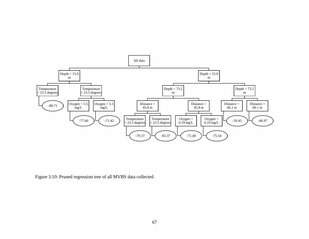
67

Figure 3.10: Pruned regression tree of all MVBS data collected.

All data

Depth < 15.0 m

Temperature < 23.5 degrees

-80.71

Temperature > 23.5 degrees

Oxygen < 5.5 mg/L

-77.60

Oxygen > 5.5 mg/L

-71.42

Depth > 15.0 m

Depth < 73.2 m

Distance < 45.8 m


-70.37


-65.37

Distance > 45.8 m

Oxygen < 6.19 mg/L

-71.40

Oxygen > 6.19 mg/L

-75.54

Depth > 73.2 m

Distance < 66.1 m

-59.45

Distance > 66.1 m

-66.97

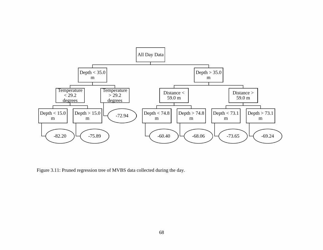
68

Figure 3.11: Pruned regression tree of MVBS data collected during the day.

All Day Data

Depth < 35.0 m


Depth < 15.0 m

-82.20

Depth > 15.0 m

-75.89


-72.94

Depth > 35.0 m

Distance < 59.0 m

Depth < 74.8 m

-60.40

Depth > 74.8 m

-68.06

Distance > 59.0 m

Depth < 73.1 m

-73.65

Depth > 73.1 m

-69.24

69

Figure 3.12: Pruned regression tree of MVBS data collected at night.

All Night Data

Oxygen < 6.0 mg/L

Depth < 75.0 m

Distance < 46.9 m

-63.92

Distance > 46.9 m

-68.12

Depth > 75.0

-55.24

Oxygen > 6.0 mg/L

Depth < 8.87 m

-80.48

Depth > 8.87 m

-71.75

70

DISCUSSION This study used hydroacoustic surveys to examine the spatial and temporal fish

biomass around lit and unlit oil and gas platforms in the northern GOM. Several acoustic

studies in the past have focused on quantifying the fish communities surrounding these

platforms in an effort to determine their value as artificial reefs (Stanley and Wilson

1996, 1997, 2000, Boswell et al. 2010, Harwell 2013, Simonsen 2013, Reynolds 2015).

As determined in these previous studies, results suggest that fish congregate close the

structure with biomass decreasing with increasing distance from the platform. The day-

only and full regression trees suggest that biomass drops off between 59.0 - 66.0 m away

from the platform. This area of influence is similar in diameter to previous studies

(Stanley and Wilson 2003, Simonsen 2013, Reynolds 2015).

Results of the mixed model showed that all of the variables tested were significant

except for platform type and season. This includes depth, distance, time of day, and all

second order interactions. However, many traditional linear regression models are

impractical for analyzing hydroacoustic data due to the large number of degrees of

freedom. For instance, Reynolds (2015) found that with nearly 100,000 degrees of

freedom, significant differences in MVBS would be detected between values as little as

<0.06% different with a confidence level of p=0.0005. Therefore, nearly every variable

examined was determined to be statistically significant, even if it did not contribute to

biological significance. Therefore, depth, distance, and time of day, while statistically

significant, may or may not have any biological significance on the system.

Results suggest that MVBS was higher at lit platforms than at unlit platforms. It is

possible that this is because fish are attracted to the artificial night lighting, especially

71

since MVBS was also higher at night. However, the night regression tree showed that

fish were avoiding the upper water column, likely in an effort to remain hidden from

nocturnal predators. Therefore, it seems unlikely that fish are attracted to lit platforms

simply because of the light field. Lit platforms tend to be larger than unlit platforms

(surface area of piles = 208,456 m2 versus 90,863 m2, respectively), which may have

some impact on MVBS. Bohnsack et al. (1994) found that fish density increased with

increasing size of the artificial reef, however, as surface area of the structure was not

selected as a variable for any of the regression trees, it is possible that size does not

entirely explain the difference in MVBS between lit and unlit platforms.

Acoustic results suggest that MVBS was highest in depth layer 3 and lowest in

depth layer 1. This agrees with previous studies (Stanley and Wilson 2003, Boswell 2010,

Reynolds 2015), which also found high biomass at depth. MVBS values at depth are

higher than those calculated by Boswell (2010) but are similar to those calculated by

Simonsen (2013), who also researched platforms in the 75-90 m depth range. At night,

the regression tree split the MVBS data at ~9 m depth. The shallowest depths showed

MVBS values nearly as low as background levels, suggesting almost no fish in the top of

the water column. There are several reasons this might be the case: they were undetected

by the acoustics or they were simply not present in the upper water column, perhaps

dispersing to distances outside of our transect range.

Fish could go undetected by acoustics for several reasons. For instance, the fish

might have sought shelter within the platform itself. Further, some fish species do not

give off strong MVBS values. The swimbladder is responsible for up to 90% of a fish’s

echo, therefore, fish species with swimbladders are more detectable than those without

72

(Foote 1980, Simmonds and MacLennan 2005). Some large predatory species, including

sharks and tunas, do not regulate buoyancy with a swimbladder. Instead, fatty livers or

constant swimming serve to buoy them in the water column (Magnuson 1973, Phleger

1998). Therefore, these fish often remain undetected by acoustics. It is possible that these

predators were present in the upper water column and were simply invisible to our

methodology, which could explain why MVBS values were so low at the surface.

Another possibility is that fish could be have been repelled by the artificial light

field. Under typical nocturnal conditions, zooplankton migrate vertically from depth to

the surface to feed on phytoplankton in the nutrient rich surface waters, drawing

planktivorous fish to the surface to feed (see Brierley 2014 for review). This suggests that

surface waters should exhibit high MVBS values. However, Simonsen (2013) sampled

acoustic biomass around oil platforms in the GOM during a 48-hour period and found a

near breakdown of diel vertical migration: instead of coming to the surface, fish were

remaining at depth. Keenan et al. (2007) found that the light from active oil and gas

platforms extended at least 10 m below the surface of the water, so it can be assumed that

the water in the top ~9 m was illuminated. The low MVBS values at the surface suggest

that fish are avoiding nocturnal predation by moving deeper into the water column, where

the water remains dark despite artificial night lighting of the platform.

Fish could also be leaving the safety of the platform entirely. MVBS was much

greater at night than during the day, especially at distances further from the platform.

This suggests that larger fish leave the protection of the platform at night. It has been well

established that red snapper nocturnally forage away from artificial reefs (Topping 2009,

Topping and Szedlmayer 2011). While these studies were conducted at small, low relief

73

reefs off the coast of Alabama rather than large oil platforms, it is possible this same

foraging behavior causes high biomass values away from the platform at night. Simonsen

(2013) found that fish biomass around GOM platforms varied with hour of the day, with

biomass near the platforms lowest at night. This may be further evidence that fish are

leaving the platform at night to forage, or that they took refuge within the platform piles

(legs) to reduce interactions with nocturnal predators.

The regression trees indicated the presence of an area of influence around the

structure ranging from ~ 45.0 – 67.0 m. Area of influence is often cited as the region of

high biomass that exists from the platform to approximately 100 m away from the

structure (Stanley and Wilson 1996, Boswell et al. 2010, Simonsen 2013, Reynolds

2015). The area of influence found in this study was cone shaped, with MVBS

concentrated closer to the structure at the surface (~45.8 m) and expanding outwards at

depth (~66.1m). These distances are within the area of influence range described in other

studies that have used acoustics around 1arge oil and gas platforms (Stanley and Wilson

1996, Wilson 2003, Simonsen 2013, Reynolds 2015). This cone shape of MVBS may be

due to the artificial light field present in the top ~10.0 m of the water column (Keenan et

al. 2007). To successfully feed in darkness, predators often position themselves below the

prey, silhouetting it against the ambient surface lighting. This includes coastal sharks,

large jacks, tunas, wahoo, and barracuda (McFarland et al. 1991, Porter and Motta 2004,

Habbegger et al. 2010), all of which are common in the GOM and were seen in large

numbers at these sites (Chapter 2). These predators are often actively foraging at night

and have an eye physiology that is adapted for low-light conditions. The artificial night

lighting of the platform provides excellent surface light with which to silhouette prey and

74

attack prey species. Therefore, small surface-oriented species such as blue runner appear

to avoid the lit portion of the water column, concentrating near or within the structure

itself.

This study utilized three split-beam mobile transducers, which allowed for

thorough data collection around the platforms. However, it missed any fish biomass

concentrated within the structure itself. Previous acoustic studies in the GOM have

utilized stationary hydroacoustics (Stanley and Wilson 1996, 1997, 2000). This is a

useful technique for hard to sample locations, but it does not give the most accurate

information for fish located farther from the platform. Ideally, both stationary and mobile

hydroacoustic surveys would be utilized to develop a more complete understanding of

fish biomass in and around the structure, respectively. It is also unlikely that the

transducer passed directly over the center of a school of fish or that the school will

conform to a perfectly round shape. Further, MVBS values are highly variable even

among fishes of the same species and size, resulting in potential underestimation

(Simmonds and MacLennan 2005). Finally, many large predators do not possess

swimbladders and are nearly invisible to hydroacoustic technology. All of these factors

will bias final biomass results by assuming fewer individuals than are actually present.

It is important to note that many studies use target strength (TS) values for their

analysis of species composition, a proxy for fish length (Simmonds and MacLennan

2005). TS is useful in regions of low species diversity, where the specific species TS

values are well established, however, it is impractical for this study design. TS is highly

dependent on water temperature, fish orientation, time of day, and other factors

(Simmonds and MacLennan 2005). The high diversity of species around oil platforms, a

75

lack of established TS values, and the close proximity of many individuals make TS

values nearly impossible to differentiate. Additionally, the species composition was

probably not the same between lit and unlit habitat types, therefore, acoustic biomass is a

better metric for this study.

There are many unexplored reasons that lit platforms are surrounded by more fish

biomass than unlit platforms. For instance, crew members on oil and gas platforms have

been observed to throw food scraps and waste over the side of the structure, thus

attracting fish (T. Tunstall, personal communication2). While the regression tree model

did not include surface area as one of the most important variables, it is still possible that

it plays a role in determining fish biomass and abundance. More consistent monitoring in

the future would be useful for determining if the differences witnessed in this study

continue over time. Due to the highly stochastic nature of environmental conditions the

GOM, it is difficult to say if the results seen here are consistent across temporal or spatial

scales, especially when platforms are distributed across great distances. The statistical

results presented should be interpreted carefully as the large sample size can obscure true

differences. Further, future work at these artificial reefs would benefit from conducting

nocturnal plankton trawls to determine if zooplankton surrounding lit platforms

experience a disturbance of their natural diel vertical migration patterns due to artificial

light effects.

While the spatial distribution of fishes around oil and gas platforms has been

described (Stanley and Wilson 1996, 1997, 2000), this is the first study to examine the

effect of light on this distribution. This study suggests that light may play a role in

2 Thomas Tunstall, captain of the Blazing 7 Research Vessel, June 2014.

76

structuring and distributing the fish community around oil and gas platforms. While fish

are attracted to the platforms’ vertical relief, they may be avoiding the nocturnal light

field emitted by lit structures in an effort to avoid predation.

LITERATURE CITED Anderson, C. I. H., A. S. Brierley, and F. Armstrong. 2005. Spatio-temporal variability in

the distribution of epi-and meso-pelagic acoustic backscatter in the Irminger Sea, North Atlantic, with implications for predation on Calanus finmarchicus. Marine Biology 146:1177-1188.

Bohnsack, J. A. 1994. Effects of reef size on colonization and assemblage structure of

fishes at artificial reefs off southeastern Florida, USA. Bulletin of Marine Science 55:796-823.

Boswell, K. M., R. J. D. Wells, J. H. Cowan, Jr., and C. A. Wilson. 2010. Biomass,


Brierley, A. S. 2014. Diel vertical migration. Current Biology 24:R1074-R1076. Bureau of Safety and Environemtnal Management (BSEE). 2015. Platform Structures

Online Query. http://www.data.bsee.gov/homepg/data_center/platform/platform/master.asp. Last accessed January 18, 2016.

Dauterive, L. 2000. Rigs-To-Reefs policy, progress, and perspective. U.S. Department of

the Interior, Minerals Management Service, Gulf of Mexico OCS Region. OCS Report MMS 2000-073.

De Robertis, A., and I. Higginbottom. 2007. A post-processing technique to estimate the

signal-to-noise ratio and remove echosounder background noise. ICES Journal of Marine Science: Journal du Conseil 64:1282-1291.

De'ath, G., and K. E. Fabricius. 2000. Classification and regression trees: a powerful yet

simple technique for ecological data analysis. Ecology 81:3178-3192. Fabi, G., and A. Sala. 2002. An assessment of biomass and diel activity of fish at an

artificial reef (Adriatic Sea) using a stationary hydroacoustic technique. ICES Journal of Marine Science: Journal du Conseil 59:411-420.

Foote, K. G. 1980. Importance of the swimbladder in acoustic scattering by fish: A

comparison of gadoid and mackerel target strengths. Journal of Acoustical Society of America. 67:2084-2089.

77

Habbegger, M. L., P. J. Motta, D. R. Huber, and S. M. Deban. 2010. Feeding

biomechanics in the Great Barracuda during ontogeny. Journal of Zoology 283:63-72.

Harwell, G. E. 2013. Acoustic biomass of fish associated with an oil and gas platform

before, during and after "reefing" it in the northern Gulf of Mexico. M.S. Thesis. Louisiana State University, Baton Rouge.

Kalikhman, I. L., and K. I. Yudanov. 2006. Acoustic Fish Reconnaissance. Taylor &

Francis Group, Boca Raton, Florida. Keenan, S. F., M. C. Benfield, and J. K. Blackburn. 2007. Importance of the artificial


Louisiana Artificial Reef Program (LARP). 2015. Artificial Reef Program.

http://www.wlf.louisiana.gov/fishing/artificial-reef-program. Last accessed June 5, 2015.

MacLennan, D. N. 1990. Acoustical measurement of fish abundance. The Journal of the

Acoustical Society of America 87:1-15. Maclennan, D. N., P. G. Fernandes, and J. Dalen. 2002. A consistent approach to

definitions and symbols in fisheries acoustics. ICES Journal of Marine Science: Journal du Conseil 59:365-369.

Magnuson, J. J. 1973. Comparative study of adaptations for continuous swimming and

hydrostatic equilibrium of scombroid and xiphoid fishes. Fishery Bulletin 71:337-356.

McFarland, W. 1991. Light in the sea: the optical world of elasmobranchs. The Journal of

Experimental Zoology Supplement. 5:3-12. Phleger, C. F. 1998. Buoyancy in Marine Fishes: Direct and Indirect Role of Lipids.

American Zoologist. 38:321-330. Porter, H. T. and P. J. Motta. 2004. A comparison of strike and prey capture kinematics

of three species of piscivorous fishes: Florida gar (Lepisosteus platyrhincus), redfin needlefish (Stongylura notate), and great barracuda (Sphyraena barracuda). Marine Biology 145:989-1000.


oil and gas platforms in the northern Gulf of Mexico using hydroacoustic and video surveys. M.S. Thesis. Louisiana State University, Baton Rouge.

78

Ripley, B. 2015. tree: Classification and Regression Trees. R package version 1.0-36. http://CRAN.R-project.org/package=tree

Simmonds, J., and D. MacLennan. 2005. Fisheries Acoustics Theory and Practice, 2nd

edition. Blackwell Science, Oxford, U.K. Simonsen, K. A. 2013. Reef fish demographics on Louisiana artificial reefs: the effects of


Soldal, A. V., I. Svellingen, T. Jørgensen, and S. Løkkeborg. 2002. Rigs-to-reefs in the

North Sea: hydroacoustic quantification of fish in the vicinity of a “semi-cold” platform. ICES Journal of Marine Science: Journal du Conseil 59(suppl):S281-S287.





Stanley, D. R., and C. A. Wilson. 2000. Variation in the density and species composition

of fishes associated with three petroleum platforms using dual beam hydroacoustics. Fisheries Research 47:161-172.

Stanley, D. R., and C. A. Wilson. 2003. Seasonal and spatial variation in the biomass and

size frequency distribution of fish associated with oil and gas platforms in the northern Gulf Of Mexico. Pages 125-153 in Stanley, D.R. and A. Scarborough-Bull, editors. Fisheries, Reefs, and Offshore Development. American Fisheries Society, Symposium 36, Bethesda, Maryland.

Topping, D. T. 2009. The use of ultrasonic telemetry to estimate residency, movement

patterns, and mortality of red snapper, Lutjanus campechanus. Ph.D. Dissertation. Auburn University, Auburn.

Topping, D. T., and S. T. Szedlmayer. 2011. Home range and movement patterns of red

snapper Lutjanus campechanus on artificial reefs. Fisheries Research 112:77-84. Wilson, C. A., A. Pierce, and M. W. Miller. 2003. Rigs and Reefs: a comparison of the


79

GENERAL SUMMARY AND CONCLUSIONS

The goal of this study was to compare and describe fish communities at lit versus

unlit oil and gas platforms, focusing on the effect of light and other environmental

variables. A concurrent study (Foss 2016) is assessing the trophic ecology of red snapper

around these same platforms using stable isotope analysis and stomach content analysis.

No study to date has examined the impact of artificial night lighting on fish community

and biomass distribution, particularly for recreationally and commercially important

species.

Chapter 2 described the temporal and spatial changes in species abundance and

fish community structure with baited remote underwater video (BRUVs). Camera arrays

recorded video at three different depths in the water column during the day, night, and

crepuscular periods. Species abundance was higher at lit platforms than at unlit platforms,

with blue runner as the dominant species at both types. A PERMANOVA indicated that

platform type, season, and depth were all important factors that affect community

structure around oil and gas platforms, which is consistent with previous studies (Rooker

et al. 1997, Stanley and Wilson 2003, Wilson 2003, Reynolds 2015).

Chapter 3 described the spatial distribution of fish biomass estimated from mobile

hydroacoustic surveys conducted during the day and at night. Spatial biomass was

calculated as mean volume backscattering strength (MVBS), a proxy for biomass. MVBS

varied with time of day, depth bins, and distance from the platform. MVBS was highest

close to the structure but declined with distance before leveling off to background levels,

which is consistent with previous studies (Stanley and Wilson 1996, 1997, 2003, Harwell

80

2013, Simonsen 2013, Reynolds 2015). MVBS was greater at depth layer 3 (>60m) than

depth layer 1 (0-30m), possibly due to a large number of red snapper at depth.

Also in Chapter 3, hydroacoustic data were examined through the use of

regression trees, which split the data into two mutually exclusive groups, with biomass

values in either ‘branch’ as homogenous as possible (De'ath and Fabricius 2000). Depth

(m), distance from platform (m) temperature (°C), and oxygen concentration (mg/L) were

detected to be significant variables by the model. Of particular interest was the night-only

data split at a depth of of ~ 9 m. This depth has been reported as the deepest extent of

light penetration from the high-pressure mercury lights atop the lit platforms (Keenan et

al. 2007). MVBS was higher in waters deeper than 9 m, and nearly non-existent in water

shallower than 9 m, indicating that fish were avoiding this lit area of the water column,

most likely in an effort to avoid predation. The video data indicated that sharks were

often present in the top 30 m of the water column at night, occurring in seven of the 11

nocturnal video drops (63.6%). The presence of these apex predators likely resulted in

teleost fish avoiding the lit portion of the water column near the surface.

By examining the results of both methodologies, I was able to gain a more

exhaustive understanding of how light impacts fish community structure and fish biomass

distribution around oil and gas platforms in the GOM. The results of both video analysis

and hydroacoustics data agree that fish are avoiding the upper water column at night,

perhaps in an effort to avoid nocturnal predation from sharks, which were common in the

video analysis. Based upon video data, average abundance of fishes was low at depth,

while acoustic data suggested that fish biomass was highest at depth. This discrepancy is

likely due to poor visibility at depth, resulting in an underestimation of fish abundance in

81

the video analysis. In the future, this problem of underestimation may be remedied by

using red light rather than white light. White light has been shown to disrupt normal fish

behaviors by initiating avoidance behavior, especially at night (Widder et al. 2005).

The combination of hydroacoustics and BRUV surveys allowed for accurate and

rapid sampling of these structures. While acoustics is not visibility limited, it has a low

resolution, indicating real biomass without resolving differences in species composition.

Meanwhile, BRUVs provide a limited field of view (often only one side of the platform)

but can be used to identify individual fish to the species level. The combination of both

techniques allows researchers to determine not only how many fish are present, but also

species relative abundance. The methodology utilized in this study has been found to be

useful for sampling platforms in previous studies (Langland 2015, Reynolds 2015) and

should be used for future monitoring of these structures.

Oil and gas platforms are useful as artificial reefs in a region where hard substrate

is limited. The structures are stable, plentiful, and serve as a continuous link from the

benthos to the photic zone. Further, they serve to congregate economically important fish

species including red snapper and greater amberjack. This study successfully

implemented both video and acoustic survey techniques to determine the area of

influence around oil and gas platforms and estimate species abundance throughout the

water column over the course of two years. The results of this study suggest that while

fish are attracted to the vertical structure of the platform, they avoid the artificial light

field near the surface, which likely puts them at a much higher risk of predation. In this

way, light can potentially impact the nocturnal landscape of fish distribution around oil

and gas platforms. However, it is unlikely that this artificial light effect plays as strong a

82

role in determining species presence and distribution as other factors, such as depth or

distance from platform.

LITERATURE CITED De'ath, G., and K. E. Fabricius. 2000. Classification and regression trees: a powerful yet

simple technique for ecological data analysis. Ecology 81:3178-3192. Foss, K. 2016. Effects of Artificial Light on the Trophic Ecology of Red Snapper Around

Standing Platforms in the Northern Gulf of Mexico. M.S. Thesis. Louisiana State University, Baton Rouge.

Harwell, G. E. 2013. Acoustic biomass of fish associated with an oil and gas platform

before, during and after "reefing" it in the northern Gulf of Mexico. M.S. Thesis. Louisiana State University, Baton Rouge.

Keenan, S. F., M. C. Benfield, and J. K. Blackburn. 2007. Importance of the artificial


Langland, T. 2015. Fish asssemblage structure, distribution, and trophic ecology at

northwestern Gulf of Mexico banks. Ph.D. dissertation. Louisiana State University, Baton Rouge.


oil and gas platforms in the northern Gulf of Mexico using hydroacoustic and video surveys. M.S. Thesis. Louisiana State University, Baton Rouge.



Simonsen, K. A. 2013. Reef fish demographics on Louisiana artificial reefs: the effects of






83

Stanley, D. R., and C. A. Wilson. 2003. Seasonal and spatial variation in the biomass and size frequency distribution of fish associated with oil and gas platforms in the northern Gulf Of Mexico. Pages 125-153 in Stanley, D.R. and A. Scarborough-Bull, editors. Fisheries, Reefs, and Offshore Development. American Fisheries Society, Symposium 36, Bethesda, Maryland.

Widder, E. A., B. H. Robison, K. R. Reisenbachler, and S. D. H. Haddock. 2005. Using

red light for in situ observations of deep-sea fishes. Deep-Sea Research Part I. 52:2077-2085.

Wilson, C. A., A. Pierce, and M. W. Miller. 2003. Rigs and Reefs: a comparison of the


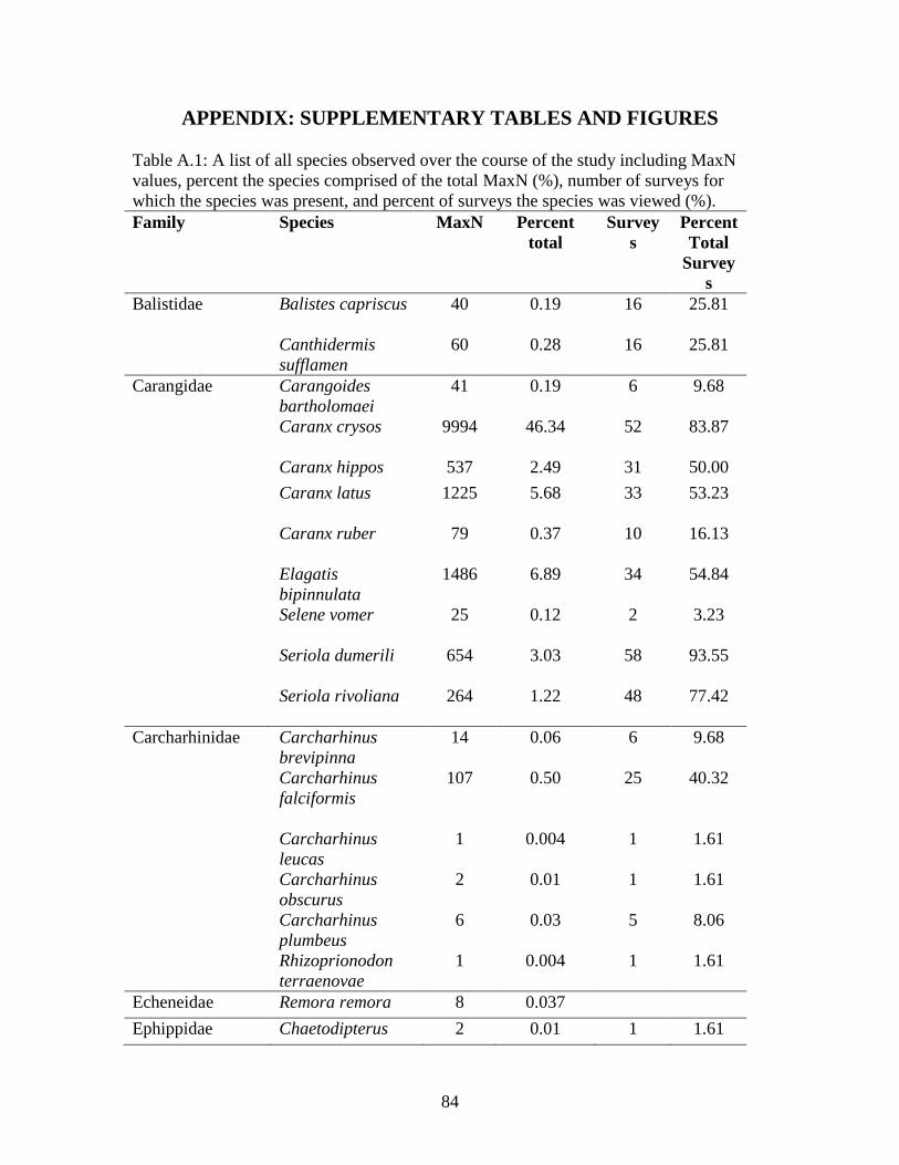
84

APPENDIX: SUPPLEMENTARY TABLES AND FIGURES Table A.1: A list of all species observed over the course of the study including MaxN values, percent the species comprised of the total MaxN (%), number of surveys for which the species was present, and percent of surveys the species was viewed (%). Family Species MaxN Percent

total Survey

s Percent Total

Surveys

Balistidae Balistes capriscus 40 0.19 16 25.81

Canthidermis sufflamen

60 0.28 16 25.81

Carangidae Carangoides bartholomaei

41 0.19 6 9.68

Caranx crysos 9994 46.34 52 83.87

Caranx hippos 537 2.49 31 50.00 Caranx latus 1225 5.68 33 53.23

Caranx ruber 79 0.37 10 16.13

Elagatis

bipinnulata 1486 6.89 34 54.84

Selene vomer 25 0.12 2 3.23

Seriola dumerili 654 3.03 58 93.55

Seriola rivoliana 264 1.22 48 77.42

Carcharhinidae Carcharhinus

brevipinna 14 0.06 6 9.68

Carcharhinus

falciformis

107 0.50 25 40.32

Carcharhinus leucas

1 0.004 1 1.61

Carcharhinus obscurus

2 0.01 1 1.61

Carcharhinus plumbeus

6 0.03 5 8.06

Rhizoprionodon terraenovae

1 0.004 1 1.61

Echeneidae Remora remora 8 0.037 Ephippidae Chaetodipterus 2 0.01 1 1.61

85

faber Holocentridae Holacanthus

ciliaris 9 0.04 3 4.84

Kyphosidae Kyphosus sectatrix 1064 4.93 38 56.45

Labridae Bodianus

pulchellus 38 0.18 4 6.45

Bodianus rufus 1 0.004 1 1.61

Clepticus parrae 1 0.004 1 1.61

Lutjanidae Lutjanus

campechanus 1691 7.84 58 93.55

Lutjanus

cyanopterus 1 0.004 1 1.61

Lutjanus griseus 112 0.52 24 38.71

Lutjanus jocu 1 0.004 1 1.61

Rhomboplites

aurorubens 214 0.99 14 22.58

Megalpidae Megalops

atlanticus 38 0.18 1 1.61

Myliobatidae Manta birostris 1 0.004 1 1.61

Pomacanthidae Holocanthus

bermudensis 4 0.02 2 3.23

Pomacanthus paru 4 0.02 2 3.23

Pomacanthus

arcuatus 1 0.004 1 1.61

Pomacentridae Abudefduf saxatilis 23 0.11 1 1.61

Rachycentridae Rachycentron

canadum 12 0.06 5 8.06

Scombridae Euthynnus

alletteratus 3205 14.86 15 24.19

Scorpaenidae

Pterois miles 4 0.02 3 4.84

Serranidae Epinephelus nigritus

4 0.02 4 6.45

Mycteroperca microlepis

3 0.014 2 3.23

Mycteroperca phenax

19 0.09 12 19.36

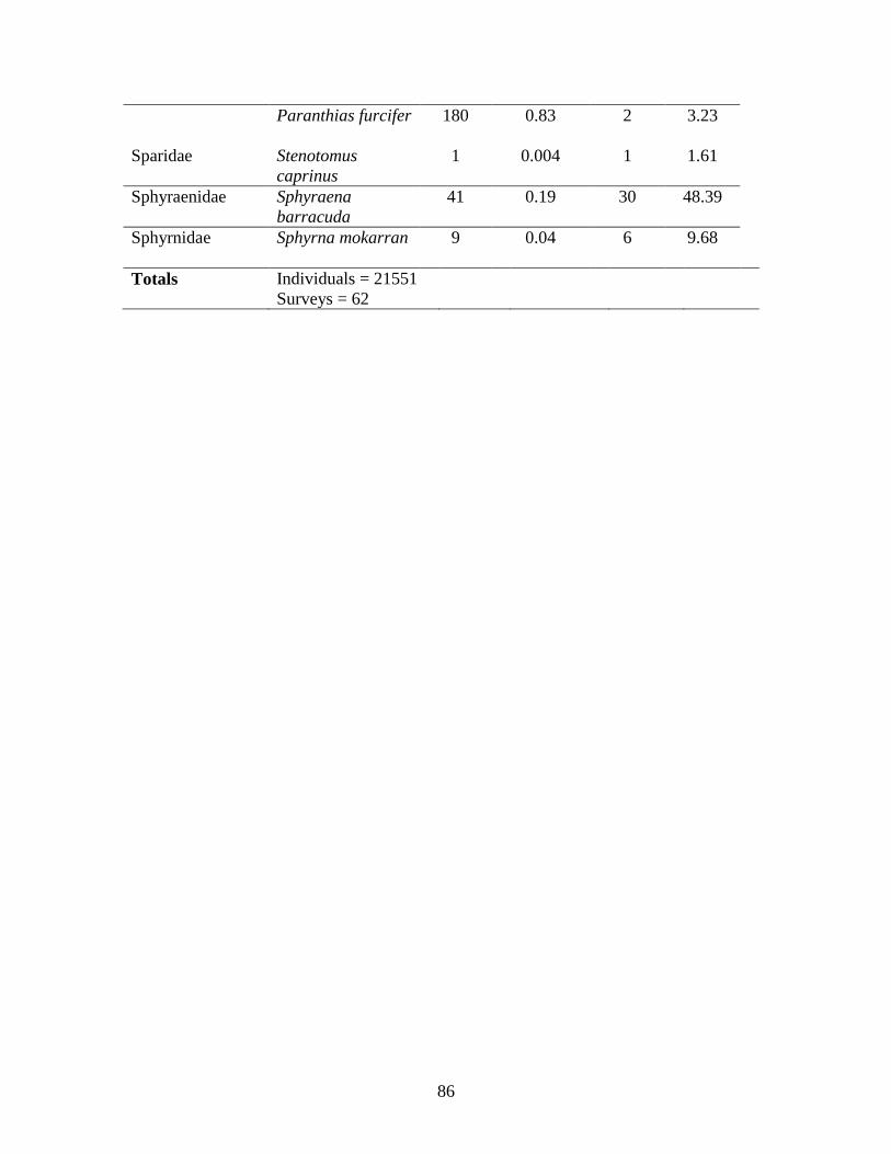
86

Paranthias furcifer 180 0.83 2 3.23

Sparidae Stenotomus caprinus

1 0.004 1 1.61

Sphyraenidae Sphyraena barracuda

41 0.19 30 48.39

Sphyrnidae Sphyrna mokarran 9 0.04 6 9.68

Totals Individuals = 21551 Surveys = 62

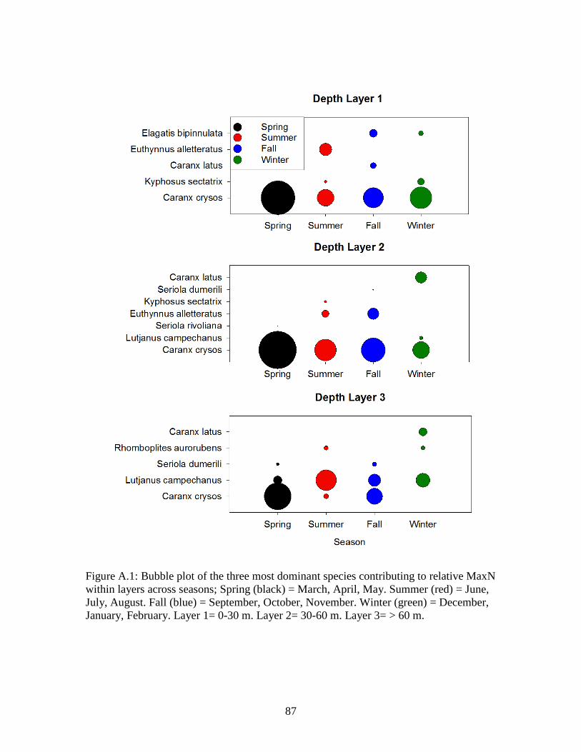
87

Figure A.1: Bubble plot of the three most dominant species contributing to relative MaxN within layers across seasons; Spring (black) = March, April, May. Summer (red) = June, July, August. Fall (blue) = September, October, November. Winter (green) = December, January, February. Layer 1= 0-30 m. Layer 2= 30-60 m. Layer 3= > 60 m.

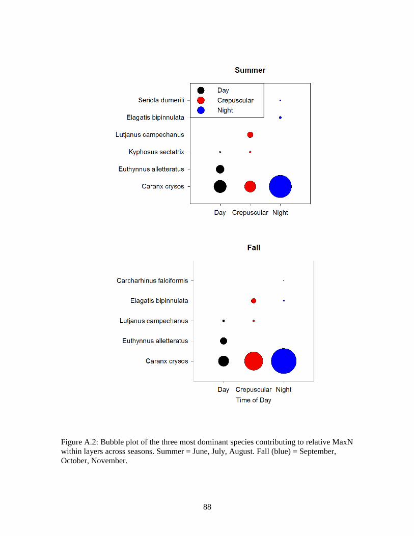
88

Figure A.2: Bubble plot of the three most dominant species contributing to relative MaxN within layers across seasons. Summer = June, July, August. Fall (blue) = September, October, November.

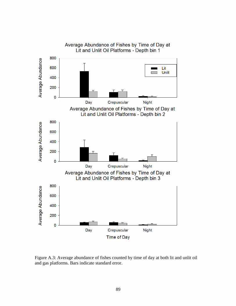
89

Figure A.3: Average abundance of fishes counted by time of day at both lit and unlit oil and gas platforms. Bars indicate standard error.

90

VITA

Victoria Barker was born in 1991 in Cincinnati, Ohio. She grew up in Liberty

Township, Ohio where she enhanced her love of the ocean by working at the Newport

Aquarium in Newport, KY. She graduated from Ursuline Academy High School in 2009

and attended the University of South Carolina in Columbia, SC. During her four years at

USC, she worked in four different laboratories researching everything from the effect of

pollutants on freshwater fish assemblages to the correlation between heavy metal

concentrations and childhood mental retardation. She spent a semester abroad at the

University of Queensland, Brisbane, Australia where she spent two weeks volunteering

on the Great Barrier Reef and working with researchers to study wave effects on tropical

sponge morphology. She received her Bachelor of Science in marine science with a

minor in biology from the University of South Carolina in May of 2013. In August 2013,

Victoria entered the Department of Oceanography and Coastal Sciences at Louisiana

State University under the supervision of Dr. James H. Cowan, Jr. She is a candidate to

receive a master’s degree in Oceanography and Coastal Sciences in May of 2016.

Documents

The Effect of Artificial Light on the Community Structure