The Economic Lot-Sizing Problem New Results and Extensions

One way for firms to reduce cost is efficient production planning. Themain theme in this thesis is a classical production planning problem:the economic lot-sizing (ELS) problem. The objective of this problemis to find a production plan that satisfies the given demand for afinite, discrete planning horizon, and minimizes the total setup, produc-tion and holding costs. We study aspects of the classical problem aswell as extensions of this problem.

In the first part of the thesis we consider the ELS model with time-in-variant cost parameters. We analyze properties of an optimal solutionand, in particular, we are interested in the proportion of holding costand setup cost in an optimal solution. Furthermore, we perform a worstcase analysis on a broad class of on-line heuristics for the problem.

Because the classical model is relatively simple, we also considerextensions of the model. We are interested whether there exist algo-rithms to solve the extensions efficiently. In the first extension weincorporate pricing decisions in the ELS model. The problem is now tofind optimal price(s) and an optimal production plan simultaneously.We consider models with variable prices and a constant price over time.

Furthermore, we extend the ELS model with a remanufacturing option.It is assumed that a known quantity of products returns from thecustomer in each period and those returned products can be remanu-factured to satisfy demand (besides regular manufacturing). Wederive algorithms and complexity results for models with a jointsetup cost for manufacturing and remanufacturing (in case of a singleproduction line) and a separate setup cost (in case of separateproduction lines).

ERIMThe Erasmus Research Institute of Management (ERIM) is the ResearchSchool (Onderzoekschool) in the field of management of the ErasmusUniversity Rotterdam. The founding participants of ERIM are RSMErasmus University and the Erasmus School of Economics. ERIM wasfounded in 1999 and is officially accredited by the Royal NetherlandsAcademy of Arts and Sciences (KNAW). The research undertaken byERIM is focussed on the management of the firm in its environment,its intra- and inter-firm relations, and its business processes in theirinterdependent connections. The objective of ERIM is to carry out first rate research in manage-ment, and to offer an advanced graduate program in Research inManagement. Within ERIM, over two hundred senior researchers andPh.D. candidates are active in the different research programs. From avariety of academic backgrounds and expertises, the ERIM communityis united in striving for excellence and working at the forefront ofcreating new business knowledge.

www.erim.eur.nl ISBN 90-5892-124-7

WILCO VAN DEN HEUVEL

The Economic Lot-Sizing ProblemNew Results and Extensions

Desig

n: B

&T O

ntw

erp en

advies w

ww

.b-en

-t.nl

Print:H

aveka ww

w.h

aveka.nl

93

WIL

CO

VA

N D

EN

HE

UV

EL

Th

e E

con

om

ic Lot-S

izing

Pro

ble

m: N

ew

Re

sults a

nd

Ex

ten

sion

s

Erim - 06 omslag vandenHeuvel 10/16/06 9:11 AM Pagina 1

1

The Economic Lot-Sizing Problem:

New Results and Extensions

2

3

The Economic Lot-Sizing Problem:

New Results and Extensions

Het economische lot-sizing probleem:

Nieuwe resultaten en uitbreidingen

PROEFSCHRIFT

ter verkrijging van de graad van doctor

aan de Erasmus Universiteit Rotterdam

op gezag van de rector magnificus

Prof.dr. S.W.J. Lamberts

en volgens besluit van het College voor Promoties.

De openbare verdediging zal plaatsvinden op

donderdag 7 december 2006 om 16:00 uur

door

Wilco van den Heuvel

geboren te Gouda.

4

Promotiecommissie

Promotor: Prof.dr. A.P.M. Wagelmans

Overige leden: Prof.dr.ir. R. Dekker

Prof.dr.ir. C.P.M. van Hoesel

Dr. H.E. Romeijn

Erasmus Research Institute of Management (ERIM)

RSM Erasmus University / Erasmus School of Economics

Erasmus University Rotterdam

Internet: http://www.erim.eur.nl

ERIM Electronic Series Portal: http://hdl.handle.net/1765/1

ERIM Ph.D. Series Research in Management, 93

ISBN–10: 90–5892–124–7

ISBN–13: 978–90–5892–124–6

Design: B&T Ontwerp en advies www.b-en-t.nl / Print: Haveka www.haveka.nl

Cover design: Janco Tolhoek

c©2006, Wilco van den Heuvel

All rights reserved. No part of this publication may be reproduced or transmitted in any

form or by any means, electronic or mechanical, including photocopying, recording, or by any

information storage and retrieval system, without permission in writing from the author.

This thesis was prepared with LATEX2e.

5

Acknowledgements

Writing a thesis is a task you do not accomplish on your own. This is a very good moment

to thank some people who (indirectly) contributed to this thesis.

First of all, I would like to thank my promotor and supervisor Albert Wagelmans.

Albert, you taught me a lot about doing research and you shaped me as a researcher. I

am still surprised you always found time to discuss my research and I really enjoyed the

Friday afternoons, when we discussed about research and new ideas for sometimes more

than two hours. Besides working with you as a researcher, I also appreciate you as a

person. To illustrate this, among other social events, we had a very pleasant time at the

Informs conference in Istanbul in 2003, when playing soccer at some tournaments, and

when having a barbecue in your backyard.

Secondly, I want to thank the other members of the inner committee, Rommert Dekker,

Stan van Hoesel and Edwin Romeijn, for evaluating this thesis. Furthermore, I thank

Zeger Degraeve, Hans Frenk and Steef van de Velde for being a member of the PhD

committee.

Of course, working environment is also important when writing a thesis. I enjoyed the

pleasant time on the 16th floor and later on the 9th floor of the H-building (the ‘PhD

floors’). We did not only have lunch together, where we discussed all kinds of topics, but

we also played darts and, of course, the game Koehandel, for which the optimal strategy

is still unknown at the time of writing. I therefore would like to thank my (former) PhD

colleagues Amy, Bjorn, Bram, Cerag, Daniel, Dennis F., Dennis H., Gabriella, Joost, Jos,

Kevin, Klaas, Lenny, Ludo, Martijn, Merel, Remco, Rene, Robin, Rutger, Sandra and

Ward. A special thanks goes to Lenny and Jos, who shared a room with me for four

years, and to my paranymphs, Robin and Rene, whom I owe apologies for the times I

disturbed them too often with the ‘4pm chats’.

Writing a thesis is not always a pleasant time, especially when you are stuck in your

research. At those times my ‘korfbal friends’ were always a good distraction. Spending

a weekend with these guys always resulted in a fresh mind for the start of the next week

(although not always in a sound body). To mention some of them I thank Ernst ‘Gordon’

Hofstede, Erwin ‘Boogie’ Kruiswijk, Erwin ‘Chupa’ Tolhoek and Janco ‘Doodle’ Tolhoek.

Furthermore, I want to thank Rachel for always being a good friend.

6

vi

Another important ‘thank you’ goes to my family, who always supported me during

my PhD trajectory (Pa, ma en Arno bedankt!). Last, but certainly not least, I want

to thank Diana for coming into my life more than a year ago. Diana, although I still

have problems explaining what I am really doing, you always supported me during the

completion of this thesis and I am very grateful for that.

Wilco van den Heuvel

Rotterdam, October 2006

7

Contents

Acknowledgements v

1 Introduction 1

1.1 General introduction and motivation . . . . . . . . . . . . . . . . . . . . . 1

1.2 Outline . . . . . . . . . . . . . . . . . . . . . . . . . . . . . . . . . . . . . . 3

I New results on the classical problem 7

2 An upper bound on the holding cost for the ELS problem with time-

invariant cost 9

2.1 Introduction . . . . . . . . . . . . . . . . . . . . . . . . . . . . . . . . . . . 9

2.2 The main result . . . . . . . . . . . . . . . . . . . . . . . . . . . . . . . . . 10

2.3 Application to heuristics . . . . . . . . . . . . . . . . . . . . . . . . . . . . 14

2.3.1 Heuristic H . . . . . . . . . . . . . . . . . . . . . . . . . . . . . . . 14

2.3.2 Heuristic H∗ . . . . . . . . . . . . . . . . . . . . . . . . . . . . . . . 15

2.3.3 An application of heuristic H . . . . . . . . . . . . . . . . . . . . . 18

2.3.4 Combining heuristic H∗ with other heuristics . . . . . . . . . . . . . 19

2.4 The constant demand case with infinite horizon . . . . . . . . . . . . . . . 19

2.4.1 Specification of H∗ . . . . . . . . . . . . . . . . . . . . . . . . . . . 20

2.4.2 Worst case analysis . . . . . . . . . . . . . . . . . . . . . . . . . . . 21

2.5 Conclusion . . . . . . . . . . . . . . . . . . . . . . . . . . . . . . . . . . . . 23

3 Performance bounds for a general class of on-line lot-sizing heuristics 25

3.1 Introduction . . . . . . . . . . . . . . . . . . . . . . . . . . . . . . . . . . . 25

3.2 Definitions, problem formulation and observations . . . . . . . . . . . . . . 27

3.3 Constructing worst case examples for heuristics satisfying Property 1 . . . 30

3.3.1 A relaxed mathematical formulation of the problem . . . . . . . . . 31

3.3.2 A special class of production plans . . . . . . . . . . . . . . . . . . 34

3.3.3 Finding the optimal demand sequence given the production plans . 38

8

viii CONTENTS

3.3.4 An initial guess for the optimal plans . . . . . . . . . . . . . . . . . 40

3.3.5 An iterative procedure to find worst case examples . . . . . . . . . 41

3.3.6 Some numerical results . . . . . . . . . . . . . . . . . . . . . . . . . 41

3.3.7 Two convergence results . . . . . . . . . . . . . . . . . . . . . . . . 44

3.4 Analysis of heuristics satisfying Properties 1-3 . . . . . . . . . . . . . . . . 47

3.4.1 A procedure to construct worst case examples . . . . . . . . . . . . 47

3.4.2 The worst case problem instance . . . . . . . . . . . . . . . . . . . 50

3.4.3 Implications . . . . . . . . . . . . . . . . . . . . . . . . . . . . . . . 53

3.5 Constructing new heuristics . . . . . . . . . . . . . . . . . . . . . . . . . . 56

3.5.1 An optimal heuristic for T = 3 . . . . . . . . . . . . . . . . . . . . . 56

3.5.2 An optimal heuristic for T = 4 . . . . . . . . . . . . . . . . . . . . . 58

3.6 Conclusion & Future research . . . . . . . . . . . . . . . . . . . . . . . . . 61

II Economic lot-sizing and pricing 63

Introduction 65

4 A joint pricing and lot-sizing model with general prices over time 67

4.1 Introduction . . . . . . . . . . . . . . . . . . . . . . . . . . . . . . . . . . . 67

4.2 Problem description . . . . . . . . . . . . . . . . . . . . . . . . . . . . . . . 68

4.3 Solution approach by Thomas (1970) . . . . . . . . . . . . . . . . . . . . . 69

4.4 Applying Thomas’ approach to the Bhattacharjee and Ramesh (2000) case 70

4.5 Intermezzo: A partition problem . . . . . . . . . . . . . . . . . . . . . . . . 73

4.5.1 Introduction . . . . . . . . . . . . . . . . . . . . . . . . . . . . . . . 73

4.5.2 Subgroups with quasiconvex average cost . . . . . . . . . . . . . . . 74

4.5.3 Subgroups with convex cost . . . . . . . . . . . . . . . . . . . . . . 76

4.6 Applying Orlin’s approach to the Bhattacharjee and Ramesh (2000) case . 77

4.7 Concerns about the results presented in Bhattacharjee and Ramesh (2000) 82

4.8 Conclusion . . . . . . . . . . . . . . . . . . . . . . . . . . . . . . . . . . . . 83

5 A joint pricing and lot-sizing problem with constant prices over time 85

5.1 Introduction . . . . . . . . . . . . . . . . . . . . . . . . . . . . . . . . . . . 85

5.2 Problem description . . . . . . . . . . . . . . . . . . . . . . . . . . . . . . . 86

5.3 Heuristic algorithm . . . . . . . . . . . . . . . . . . . . . . . . . . . . . . . 88

5.4 Exact algorithm . . . . . . . . . . . . . . . . . . . . . . . . . . . . . . . . . 90

5.5 Time complexity of the algorithm . . . . . . . . . . . . . . . . . . . . . . . 94

5.5.1 Improvement on the result of Gilbert (1999) . . . . . . . . . . . . . 94

5.5.2 Time complexity of the general problem . . . . . . . . . . . . . . . 95

5.5.3 An Ω(T 2) example . . . . . . . . . . . . . . . . . . . . . . . . . . . 101

9

CONTENTS ix

5.6 Concluding remarks . . . . . . . . . . . . . . . . . . . . . . . . . . . . . . . 105

5.A Appendix . . . . . . . . . . . . . . . . . . . . . . . . . . . . . . . . . . . . 106

III Economic lot-sizing with a remanufacturing option 107

Introduction 109

6 The economic lot-sizing problem with a remanufacturing option and

joint setup cost 111

6.1 Problem description and mathematical model . . . . . . . . . . . . . . . . 111

6.2 The time-invariant cost case . . . . . . . . . . . . . . . . . . . . . . . . . . 113

6.2.1 Structural properties of an optimal solution . . . . . . . . . . . . . 113

6.2.2 A dynamic programming algorithm . . . . . . . . . . . . . . . . . . 115

6.3 The pure remanufacturing case . . . . . . . . . . . . . . . . . . . . . . . . 118

6.3.1 Model formulation . . . . . . . . . . . . . . . . . . . . . . . . . . . 118

6.3.2 A dynamic programming algorithm . . . . . . . . . . . . . . . . . . 120

6.3.3 Improving the running time of the DP algorithm . . . . . . . . . . 123

6.3.4 Equivalence with the ELS problem with bounded inventory . . . . . 125

6.4 Open problem: the general case . . . . . . . . . . . . . . . . . . . . . . . . 126

6.5 Conclusion . . . . . . . . . . . . . . . . . . . . . . . . . . . . . . . . . . . . 128

7 Lot-sizing and remanufacturing: the separate setup cost case 129

7.1 Problem description and mathematical model . . . . . . . . . . . . . . . . 129

7.2 Complexity results . . . . . . . . . . . . . . . . . . . . . . . . . . . . . . . 130

7.2.1 The general ELSR problem . . . . . . . . . . . . . . . . . . . . . . 130

7.2.2 The ELSR problem with a disposal option . . . . . . . . . . . . . . 132

7.2.3 The ELSRD problem with fixed ending inventories . . . . . . . . . 134

7.3 Properties of an optimal solution . . . . . . . . . . . . . . . . . . . . . . . 137

7.4 A DP algorithm for the ELSR problem with given production periods . . . 138

7.4.1 Introduction . . . . . . . . . . . . . . . . . . . . . . . . . . . . . . . 138

7.4.2 The different types of regeneration intervals . . . . . . . . . . . . . 140

7.4.3 Calculating the cost for different types of regeneration intervals . . 142

7.4.4 The interval that satisfies the ZI property for serviceables . . . . . . 145

7.4.5 The recursion formulas . . . . . . . . . . . . . . . . . . . . . . . . . 146

7.5 Application of the DP algorithm to a genetic algorithm . . . . . . . . . . . 146

7.5.1 Description of the GA algorithm . . . . . . . . . . . . . . . . . . . . 147

7.5.2 Numerical results . . . . . . . . . . . . . . . . . . . . . . . . . . . . 148

7.6 Conclusion . . . . . . . . . . . . . . . . . . . . . . . . . . . . . . . . . . . . 150

10

x CONTENTS

8 Summary of the main results 153

Nederlandse samenvatting (Summary in Dutch) 157

Bibliography 161

Author index 167

Curriculum Vitae 169

11

Chapter 1

Introduction

1.1 General introduction and motivation

The economic order quantity (EOQ) model is probably the most well-known model in

inventory theory. Although the economic lot-sizing model is not as well-known as the

EOQ model, it has been of great influence in (deterministic) production and inventory

planning literature. At the celebration of “50 years of Management Science” (one of the

leading journals in Operations Research and Management Science) in 2004, the seminal

paper on the economic lot-sizing model by Wagner and Whitin (1958) was voted among

the ten most influential papers (by INFORMS members). Moreover, it was number two

on the list of most cited papers (592 citations).

The economic lot-sizing model will be the main theme in this thesis. We will study

issues related to this classical model as well as extensions of the model. In the literature

the model is also known as the dynamic lot-sizing model, where ‘dynamic’ refers to the

dynamic nature of the demand in contrast to the constant demand rate as assumed in the

EOQ model. In this thesis we will refer to the model as the economic lot-sizing (ELS)

model.

Whereas in the EOQ model (Harris, 1913) it is assumed that there is infinite time

horizon with a constant demand rate over time, in the ELS model there is discrete and

finite time horizon with in each period a (possibly different) quantity of demand. This

demand has to be satisfied by ordering in such a way that total costs are minimized.

Costs include a fixed order cost for each period an order is made, a unit cost for each

item purchased and a unit cost for each time period an item is held in stock. Instead of

considering the model in an ‘ordering environment’, the model can also be considered in

a ‘production environment’. In this case demand has to be satisfied by producing items.

Besides holding cost, there is a fixed setup cost associated with each production period

and a unit cost for each item produced.

12

2 Introduction

Because the ELS model is relatively simple and because of new developments in pro-

duction and inventory management during the last decades, several extensions of the ELS

model have been proposed in the literature. Examples of extensions are:

• more general cost functions (e.g., Zangwill (1968), Chan et al. (2002)),

• capacity constraints on production (e.g., Florian et al. (1980), Bitran and Yanasse

(1982), Van den Heuvel and Wagelmans (2006a)) and inventory (e.g., Love (1973),

Atamturk and Kucukyavuz (2005)),

• multiple items (e.g., Eppen and Martin (1987), Federgruen et al. (2006), Jans and

Degraeve (2006)),

• integration of decisions at different levels of the supply chain (e.g., Zangwill (1969),

Van Hoesel et al. (2005)),

• incorporation in game theoretical models (e.g., Federgruen and Meissner (2005),

Van den Heuvel et al. (2007)).

For surveys on lot-sizing models we refer to Kuik et al. (1994), Drexl and Kimms (1997),

Brahimi et al. (2006) and Jans and Degraeve (2007). In this thesis we will study two

other extensions of the ELS model.

In the first extension we include pricing decisions in the ELS model. The demand that

a manufacturer has to satisfy is usually created by activities of its marketing department

(assuming that the manufacturer has some market power). Instead of taking the market-

ing and production decisions more or less independently, it may be beneficial to integrate

these decisions. This leads to a model that is more complex than when we are only con-

cerned with optimal production decisions. As an example, suppose that the selling price

of the item still has to be set and that the demand functions are given for the periods

under consideration. Then the planning problem consists of deciding simultaneously how

high to set the price and how much to produce in each period such that the total profit

is maximized. In this thesis we will consider a joint pricing and lot-sizing model, where

demand is assumed to be a deterministic function of price.

In the second extension we incorporate a remanufacturing option in the ELS model.

Because of environmental legislation and for economic reasons, companies take back used

products from the customer more often. These returned products can be reused in the

production process, which is known as a type of ‘reversed logistics’. Instead of making new

products from scratch, it may be cheaper to remanufacture returned items. Therefore,

we develop a model where demand can be satisfied by manufacturing new items or by

remanufacturing returned items.

13

1.2 Outline 3

1.2 Outline

This thesis consists of three parts, where in turn each part consists of two chapters. The

chapters are written such that they can be read more or less independently. To this end,

each chapter starts with an abstract.

In Part I of this thesis we will focus on the classical ELS model with time-invariant

cost parameters. In Chapter 2 we are interested in the composition of holding cost and

order cost in an optimal solution. It is a well-known property for the EOQ model that

holding cost and order cost are equal in an optimal order cycle. The question is whether

this property also holds to some extent for the ELS model. In particular, we are interested

whether there exists a bound on the total holding cost in an optimal order interval, where

an order interval is defined as a consecutive number of periods for which demand is

satisfied by a single order.

The analysis of the above problem resulted in the development of a new heuristic for

the ELS problem. In the last part of Chapter 2 we analyze the worst case performance of

this heuristic and derive some theoretical properties. Unfortunately, it turns out that the

heuristic does not generate optimal solutions in the constant demand case (in contrast to

several other heuristics). Therefore, we perform a worst case analysis on the algorithm

for this case.

In Chapter 3 we analyze the performance of a general class of heuristics for the ELS

problem with time-invariant cost parameters. Although the ELS problem can be solved

to optimality in polynomial time, many heuristics have been proposed in the literature.

One of the reasons for this is that the ELS problem is often solved in a so-called rolling

horizon environment. That is, only demands (or demand estimates) for a limited number

of periods (the planning horizon) are known. In this case the ELS problem is solved for

the planning horizon and the first production decision is implemented in the production

schedule. Then the horizon is ‘rolled forward’ to the period where the next decision has

to be made. In this way a complete production schedule for the ‘real’ horizon can be

constructed. It turns out that solving the ELS problem for the short planning horizon by

a heuristic may result in better schedules for the real horizon (Stadtler, 2000) than when

the problem in the short planning horizon is solved to optimality.

We analyze a class of heuristics which is suitable to be applied in a rolling horizon en-

vironment, because decisions are made on a period-by-period basis. By this property the

heuristics can be considered as on-line heuristics, since decisions are made while not all

future information is known (or used). We develop procedures to systematically construct

worst case instances for a fixed time horizon and use them to derive worst case problem

14

4 Introduction

instances for an infinite time horizon.

In Part II of this thesis we extend the ELS model by incorporating pricing decisions.

We start this part with a general introduction and provide an overview on the literature

most related to the integration of pricing and lot-sizing decisions.

In Chapter 4 we consider an ELS model in which it is assumed that a manufacturer

can affect his demand by pricing, where in each period demand is a (deterministic) func-

tion of price. The problem is now to decide simultaneously how much to produce and

what prices to set in each period such that total profit is maximized. In this chapter we

focus on a special case of the problem with time-invariant demand and cost parameters

considered by Bhattacharjee and Ramesh (2000). They proposed two heuristics for the

problem. However, we show that the problem can be solved to optimality by applying

existing results in the literature. Application of (a slight modification of) the approach

by Thomas (1970) solves the problem in a (practically) efficient way. Moreover, a faster

algorithm can be developed by applying the results on a special partition problem derived

by Orlin (1985).

In Chapter 5 we impose an additional restriction on the pricing model of Chapter 4.

In practice it may not be desirable to set different prices in each time period, because

customers may speculate on price changes or price changes may be expensive to commu-

nicate to the customers. Therefore, we consider a model with the restriction that prices

must be constant over time. Kunreuther and Schrage (1973) proposed a heuristic algo-

rithm for this problem, while Gilbert (1999) proposed a polynomial time algorithm for a

special case of the problem. In this chapter, we generalize the work of Kunreuther and

Schrage (1973) and Gilbert (1999) by developing a polynomial time algorithm for the

general problem.

In Part III we allow for a remanufacturing option in the ELS model. We assume that

products return from the customers and these returned products can be remanufactured

to satisfy demand (in addition to ‘normal’ manufacturing). We start this part of the thesis

with a general introduction and an overview of the literature on lot-sizing models with a

remanufacturing option.

In the model of Chapter 6 we assume that there is a joint setup cost in each period that

manufacturing or remanufacturing occurs. This can be the case when manufacturing and

remanufacturing are performed on the same production line. We will develop an efficient

algorithm to solve this problem under the assumption of time-invariant cost parameters.

Furthermore, we show the relation between the ELS problem with a remanufacturing

15

1.2 Outline 5

option and the ELS problem with capacities on inventory.

In Chapter 7 we consider a similar model as in Chapter 6 except that we assume

a separation in setup cost. In this model there is a setup cost for both manufacturing

and remanufacturing. This may be the case when manufacturing and remanufacturing

are performed on different production lines. It turns out that under this assumption the

problem becomes more complicated. We will show that the problem is already NP-hard

in the case of time-invariant cost parameters. Furthermore, we will derive complexity

results for some related problems. Finally, we will develop a genetic algorithm for the

problem and test it by performing a numerical experiment.

The thesis is ended in Chapter 8. In this chapter we give an overview of the main

results.

16

17

Part I

New results on the classical problem

18

19

Chapter 2

An upper bound on the holding cost

for the economic lot-sizing problem

with time-invariant cost parameters

Abstract

In this chapter we derive a new property for an optimal solution of the economic lot-

sizing problem with time-invariant cost parameters. We show that the total holding

cost in an order interval of an optimal solution is bounded from above by a quantity

proportional to the setup cost and the logarithm of the number of periods in the

interval. Furthermore, we show how this property may be used for the improvement

of existing heuristics and for the development of new heuristics. We propose a new

heuristic with worst case ratio 2. Furthermore, we show the relation between the

number of setups generated by the heuristic and an optimal procedure.

2.1 Introduction

The Economic Order Quantity (EOQ) model is probably the most well-known model in

inventory management. There is a constant demand rate D over a continuous infinite

horizon, which has to be satisfied by placing orders. For every order there is an order

cost K and there is a holding cost h for each item held in inventory for a time unit. If an

order occurs every T periods, then the average cost per time unit equals

K

T+

1

2ThD,

where the fist part represents the order cost and the second part represents the holding

cost. The optimal length between two orders that minimizes the average cost equals

20

10 An upper bound on the holding cost for the ELS problem with time-invariant cost

T ∗ =√

2KDh

. It is a well-known property that setup cost and holding cost are equal for

this solution.

In this chapter we consider the discrete version of the EOQ model introduced by

Wagner and Whitin (1958), which is often referred to as the economic lot-sizing (ELS)

problem in the literature. The model has a finite and discrete time horizon of T periods

and in each period t there is a demand dt (t = 1, . . . , T ). As in the EOQ model we have a

fixed setup cost K, unit holding cost h and no unit production cost. (Note that the terms

setup cost and order cost are both used in the literature dependent on the context of the

problem.) The problem is to determine the order periods and quantities such that total

costs are minimized. Although the ELS problem can be solved efficiently, many heuristics

have been proposed in the literature. A number of those heuristics utilizes some optimality

property of the EOQ model. For example, the Silver-Meal (SM) heuristic minimizes the

cost per period, the Least Unit Cost (LUC) heuristic minimizes the cost per item, and

the Part Period Balancing (PPB) heuristic balances setup cost and holding cost.

In this chapter we are interested in the question whether the properties of the EOQ

model also hold for the ELS problem (to some extent) and hence whether it is justified to

apply heuristics based on such properties. In particular, we are interested in the relation

between holding cost and setup cost in an optimal solution. Clearly, we can have zero

holding cost in case setup cost is sufficiently small (resulting in an optimal solution with an

order in each period). This raises the question whether there also exist problem instances

for which the total holding cost is relatively large compared to the total setup cost.

In this chapter we will show that the total holding cost in an optimal order interval

is bounded from above by a quantity proportional to the setup cost and the logarithm

of the number of periods in the interval. An order interval is defined as the number of

consecutive periods for which demand is satisfied by a single order. In Section 2.2 we will

derive this bound. In Section 2.3 we show how this property can be used for the design

of heuristics. We propose two new heuristics, analyze the worst case performances, and

derive a property on the number of setups. In Section 2.4 we analyze the performance of

the best of the two heuristics for the constant demand case. The chapter is completed in

Section 2.5 with the conclusion.

2.2 The main result

It is well known that there exists an optimal solution for the ELS problem that satisfies

the zero-inventory property, i.e., a new order is placed only if the inventory drops down

to zero. This means that in any order period demand is ordered for an integral number

of consecutive periods. Consider some order interval in an optimal solution and w.l.o.g.

assume it consists of periods 1, . . . , t. In this section we will derive an upper bound on the

21

2.2 The main result 11

total holding costs in these periods. The idea of the proof is that in an optimal solution

it is never profitable to add a setup in any period p + 1 with p ∈ 1, . . . , t− 1. The total

holding cost for the order interval of length t equals

H(t) = ht∑

i=2

(i − 1)di.

Furthermore, adding a setup in period p + 1 leads to a saving in holding cost of

ph

t∑

i=p+1

di.

The following lemmas are used to derive our main theorem.

Lemma 2.1 Assume there exists a constant c ≥ 0 and a period p ∈ 1, . . . , t − 1 such

that

cph

t∑

i=p+1

di ≥ h

t∑

i=2

(i − 1)di. (2.1)

Then in an optimal solution H(t) ≤ cK.

Proof Assume that H(t) > cK. Then it follows that

ph

t∑

i=p+1

di ≥H(t)

c> K.

Now adding a setup in period p + 1 leads to a solution with cost

K + H(t) + K − ph

t∑

i=p+1

di < K + H(t).

This means that an additional setup in period p + 1 leads to a cost reduction, which

contradicts the fact that the order interval is part of an optimal solution.

It follows from Lemma 2.1 that if we can find a c that satisfies (2.1) for all demand

sequences d = d1, . . . , dt, then we have found a bound on the total holding cost in an

order interval. Note that a trivial upper bound on c is t − 1. It is easy to see that (2.1)

holds for c = t− 1 and p = 1, which implies that H(t) ≤ (t− 1)K in an optimal solution.

However, this upper bound on the holding cost is immediately obtained from the solution

with setups in periods 2, . . . , t. Because the order interval is part of an optimal solution,

holding cost must be smaller than the cost of the solution with a setup in each period.

So we are looking for a bound c that is lower than this trivial bound. In the following

lemma we will give a lower bound on the value of c and Lemma 2.3 shows that this bound

is tight.

22

12 An upper bound on the holding cost for the ELS problem with time-invariant cost

Lemma 2.2 Given the demand sequence d0 defined by

d01 > 0,

d0i = 1

i(i−1)= 1

i−1− 1

i, i = 2, . . . , t − 1

d0t = 1

t−1.

Then for the sequence d0 it holds(

t−1∑

i=1

1

i

)

p

t∑

i=p+1

d0i =

t∑

i=2

(i − 1)d0i for p = 1, . . . , t − 1.

Proof First, it holds that

t∑

i=2

(i − 1)d0i =

t−1∑

i=2

1

i+ 1 =

t−1∑

i=1

1

i.

Second, for any period p ∈ 1, . . . , t − 1 it holds

p

t∑

i=p+1

d0i = p

(t−1∑

i=p+1

(1

i − 1− 1

i

)+

1

t − 1

)

= p

((1

p− 1

t − 1

)+

1

t − 1

)= 1,

which completes the proof.

Note that for the problem instance of Lemma 2.2, adding a setup to any period p leads

to the same reduction in holding cost. Because the problem instance of Lemma 2.2 is a

specific problem instance, for an arbitrary instance we must have c ≥∑t−1i=1

1i. However,

the following lemma shows that the bound∑t−1

i=11i

is tight.

Lemma 2.3 For any demand sequence d = d1, . . . , dt there exists a period p ∈ 1, . . . , t−1 such that (

t−1∑

i=1

1

i

)p

t∑

i=p+1

di ≥t∑

i=2

(i − 1)di. (2.2)

Proof In case di = 0 for i = 2, . . . , t the lemma trivially holds. Let α > 0 be such that

t∑

i=2

(i − 1)di = αt∑

i=2

(i − 1)d0i

and define

∆d = d − αd0.

Then it holdst∑

i=2

(i − 1)∆di =

t∑

i=2

(i − 1)(di − αd0i ) = 0.

23

2.2 The main result 13

By Lemma 2.2 it is now sufficient to show that there exists a period p ∈ 1, . . . , t − 1such that

pt∑

i=p+1

di ≥ pt∑

i=p+1

αd0i ⇔ p

t∑

i=p+1

∆di ≥ 0, (2.3)

because then(

t−1∑

i=1

1

i

)p

t∑

i=p+1

di ≥(

t−1∑

i=1

1

i

)p

t∑

i=p+1

αd0i = α

t∑

i=2

(i − 1)d0i =

t∑

i=2

(i − 1)di.

Assume that (2.3) does not hold, i.e., for all p ∈ 1, . . . , t − 1

pt∑

i=p+1

∆di < 0 ⇔t∑

i=p+1

∆di < 0.

But then

0 >

t−1∑

p=1

t∑

i=p+1

∆di =

t∑

i=2

i−1∑

p=1

∆di =

t∑

i=2

(i − 1)∆di = 0,

which is a contradiction.

We are now ready to state our main theorem.

Theorem 2.4 Let periods 1, . . . , t be an order interval in an optimal solution of a problem

instance with demand sequence d1, . . . , dt. Then it holds for the total holding cost

H(t) = h

t∑

i=2

(i − 1)di ≤ K

t−1∑

i=1

1

i. (2.4)

Proof By Lemma 2.3 we have that for any problem instance (2.2) holds. Applying

Lemma 2.1 with c =∑t−1

i=11i

gives the result.

To derive the bound on the holding cost in an optimal order interval we used the fact that

one additional setup in some period can never decrease the total cost. A result by Van

Hoesel and Wagelmans (2000) shows that adding more than one setup cannot lead to a

cost reduction either. Namely, Van Hoesel and Wagelmans (2000) show that the function

z(n) is convex, where z(n) is the optimal cost of the lot-sizing problem with exactly n

setups.

A direct consequence of Lemma 2.2 is that there exists problem instances for which

the ratio between holding cost and setup cost becomes arbitrarily large. Namely, for the

problem instance with demand d0, K = 1, h = 1 and T periods an optimal solution is

to have only one setup in period 1. For this instance the ratio equals∑T−1

t=11t→ ∞ as

T → ∞. So we have the following theorem.

24

14 An upper bound on the holding cost for the ELS problem with time-invariant cost

Theorem 2.5 There exist problem instances for which the ratio between holding cost and

setup cost in an optimal solution is arbitrarily large.

Theorem 2.5 shows that the PPB criterium is not justified because holding cost and setup

cost need not be balanced in an optimal solution.

Finally, note that the sum of the first t − 1 terms of the harmonic series∑t−1

i=11i

increases relatively slowly. It is well known that

limn→∞

(n∑

i=1

1

i− log n

)= γ,

where γ = 0.577 . . . is the Euler-Mascheroni constant. Using this result it is not difficult

to show thatt−1∑

i=1

1

i≤ γ + log t. (2.5)

So using (2.4) and (2.5) the holding cost of any optimal order interval satisfies

H(t) ≤ K(γ + log t), (2.6)

which means that the holding cost equals at most a quantity proportional to the setup

cost and the logarithm of the number of periods in the order interval.

2.3 Application to heuristics

2.3.1 Heuristic H

Theorem 2.4 immediately suggests a new heuristic for the economic lot-sizing problem

with time-invariant costs. The heuristic selects an order interval that covers periods

1, . . . , t with t the largest period that satisfies

h

t∑

i=2

(i − 1)dt ≤ K

t−1∑

i=1

1

i. (2.7)

In this way the solution possesses a property that is satisfied by any optimal solution. We

will call this heuristic H . Unfortunately, the following example shows that the worst case

performance of H can be arbitrarily bad.

Example 2.6 Consider a problem instance with d1 > 0, dT = Kh(T−1)

∑T−1t=1

1t

and dt = 0

for t = 2, . . . , T − 1. Then the heuristic H generates a solution with only a setup in

period 1 having a total cost of CH = K + K∑T−1

t=11t. However, the optimal solution is

25

2.3 Application to heuristics 15

to order in periods 1 and T with a total cost of C∗ = 2K. Clearly, the worst case ratio

equals

CH

C∗=

K(1 +∑T−1

t=11t)

2K→ ∞ as T → ∞.

2.3.2 Heuristic H∗

In Example 2.6 we used c =∑t−1

i=11i, which is the smallest c that satisfies (2.1) for an

arbitrary problem instance. However, this is not the best value of c given a specific

problem instance. We can improve H by dynamically updating c. The implied heuristic

works as follows. Assume that we arrive in some period t with the last setup in period 1.

Calculate the smallest c that satisfies (2.1), say ct, and check whether

ht∑

i=2

(i − 1)dt ≤ ctK. (2.8)

If the latter inequality holds, proceed with period t + 1. Otherwise, make an order that

covers periods 1, . . . , t − 1, start a new order in period t and proceed with period t + 1.

We will call this heuristic H∗, the ‘refined’ version of heuristic H .

Heuristic H∗ has a nice interpretation. Note that if we arrive in some period t that

does not satisfy (2.8), then there exists some period p ∈ 2, . . . , t such that an additional

setup in period p leads to a cost reduction. So heuristic H∗ chooses the order intervals

as large as possible (except for possibly the last order interval) such that no additional

setup may improve the solution. We will use this interpretation to determine the worst

case performance of H∗.

Theorem 2.7 The worst case performance of H∗ is at most 2.

Proof Consider a solution for some arbitrary instance d generated by H∗ with cost CH∗

.

Modify this solution by adding a setup in each setup period of the optimal solution (if

none yet) and modify the order quantities accordingly. Denote the cost of this solution

by C. Assume that there are n∗ setups in the optimal solution so that we add at most

n∗ − 1 setups (both solutions have a setup in period 1) to our heuristic solution. Then

we have

CH∗ ≤ C ≤ C∗ + (n∗ − 1)K ≤ 2C∗

with C∗ the cost of the optimal solution. The first inequality follows because by definition

of our heuristic, adding setups to the heuristic solution cannot improve the solution. The

second inequality holds because the new solution has at most n∗ − 1 additional setups

and less holding cost compared to the optimal solution. Furthermore, the last inequality

holds because C∗ ≥ Kn∗. In conclusion, we have CH∗

C∗≤ 2.

26

16 An upper bound on the holding cost for the ELS problem with time-invariant cost

The following example shows that this bound is tight.

Example 2.8 Consider a problem instance with T = 2n (n ∈ N), K = h = 1, dt = 2ε

for t odd and dt = 1 − ε for t even. For ε sufficiently small heuristic H∗ generates a

solution with setups in periods 1, 3, . . . , T − 1 with total cost

CH∗

= nK + nh(1 − ε) = 2n − nε.

However, an alternative solution with setup periods 1, 2, 4, . . . , T has a total cost of

CA = (n + 1)K + 2hε(n − 1) = (n + 1) + 2(n − 1)ε.

If C∗ is the cost of the optimal solution, then the worst case ratio satisfies

CH∗

C∗≥ CH∗

CA=

2n − nε

(n + 1) + 2(n − 1)ε→ 2 for ε =

1

nand n → ∞.

Theorem 2.7 and Example 2.8 show that H∗ is a heuristic with worst case ratio 2. This

is the best possible worst case ratio for the class of heuristics in which H∗ is contained

(see Chapter 3). Note that H∗ is not contained in the class of heuristics considered by

Axsater (1985) and hence the result cannot be derived from this paper. Theorems 2.9

and 2.10 show that H∗ possesses some other nice properties.

Theorem 2.9 The number of setup periods generated by H∗ is at most the number of

setup periods in any optimal solution.

Proof Consider some order interval r, . . . , s − 1 of an optimal solution. It is sufficient

to show that H∗ will generate at most one setup in this interval. Assume this is not the

case and let v and w be two consecutive setup periods of the heuristic solution such that

r ≤ v < w < s. By definition of H∗ there exists a period p ∈ v + 1, . . . , w such that

K + h

p−1∑

i=v+1

(i − v)di + K + h

w∑

i=p+1

(i − p)di < K + h

w∑

i=v+1

(i − v)di,

which implies

K + h

p−1∑

i=r+1

(i − r)di + K + h

w∑

i=p+1

(i − p)di < K + h

w∑

i=r+1

(i − r)di.

27

2.3 Application to heuristics 17

Now add a setup in period p in the optimal solution. Then the interval r, . . . , s− 1 has a

cost of

K + h

p−1∑

i=r+1

(i − r)di + K + hs−1∑

i=p+1

(i − p)di =

K + h

p−1∑

i=r+1

(i − r)di + K + h

w∑

i=p+1

(i − p)di + h

s−1∑

i=w+1

(i − p)di <

K + h

w∑

i=r+1

(i − r)di + h

s−1∑

i=w+1

(i − p)di ≤ K + h

s−1∑

i=r+1

(i − r)di,

where the last inequality follows from p > r. This means we have found a better solution

than the optimal solution, which is a contradiction.

Theorem 2.10 Let r, . . . , s−1 be some order interval generated by H∗. Then an optimal

solution with minimum number of setups has at most 2 setups in this interval.

Proof Assume we have an optimal solution with consecutive setups in periods u < v < w

with u ≥ r and w ≤ s − 1 and minimum number of setups. By definition of optimality

we have

(v − u)

w−1∑

i=v

di > K.

That is, the additional cost of removing the setup in period v is larger than the setup

cost. Note that we have strict inequality because we assume it is an optimal solution with

minimum number of setups. Because r ≤ u

(v − r)

w−1∑

i=v+1

di ≥ (v − u)

w−1∑

i=v+1

di > K.

This means that adding a setup in period v in the solution generated by H∗ would lead

to cost reduction and hence H∗ should have a setup in period w − 1 < s − 1. But this is

a contradiction with our initial assumption.

Theorem 2.11 Let n∗ be the minimum number of setups in an optimal solution and let

n be the number of setups generated by H∗. Then n ≤ n∗ ≤ 2n or 12n∗ ≤ n ≤ n∗.

Proof Immediate from Theorems 2.9 and 2.10.

A consequence of Theorem 2.11 is that heuristic H∗ will not suffer from generating too

many setups compared to the number of setups in an optimal solution. Furthermore, the

28

18 An upper bound on the holding cost for the ELS problem with time-invariant cost

number of setups is not less than half the number of setups of an optimal solution (with

minimum number of setups).

We end this section with some remarks about H∗. First, heuristic H∗ can also be

adapted for the case of time-varying holding cost by using the interpretation that the

heuristic generates order intervals covering as many demand periods as possible such that

no additional setup may improve the solution. Similar arguments as used in the proof

of Theorem 2.7 show that this heuristic also has a worst case performance of 2. Second,

heuristic H∗ can be implemented in a backward way having the same worst case perfor-

mance. These additional properties are similar to the properties of the heuristic presented

in Bitran et al. (1984). This heuristic starts a new order if total holding cost in the current

order interval exceeds the setups cost. Finally, heuristic H∗ can be implemented in linear

time since there exists a linear time algorithm for the economic lot-sizing problem with

time-invariant costs (see, for instance, Federgruen and Tzur (1991)).

2.3.3 An application of heuristic H

In this section we apply heuristic H to a problem instance presented in Axsater (1982).

This instance is used to show that the SM-heuristic has an infinite worst case performance.

We construct a solution based on H and compare it with the SM solution. The problem

instance has a demand d1 > 0 and dt = K(t−1)h

for t = 2, 3 . . . , T . The SM heuristic

generates a solution with one setup, resulting in a cost of CSM = TK, that is a cost of K

per period.

We will now construct a solution for this problem instance based on heuristic H .

Assume period p is the last setup period of the current order interval. Then H searches

for the largest period t that satisfies

ht∑

i=2

(i − 1)di+p−1 = Kt∑

i=2

i − 1

i + p − 2≤ K

t−1∑

i=1

1

i. (2.9)

Note that (2.9) is certainly satisfied when the largest term at the left hand side of (2.9)

is smaller than the smallest term at the right side, i.e., when

t − 1

t + p − 2≤ 1

t − 1⇔ t2 − 3t + 3 + p ≤ 0. (2.10)

The length of the largest order interval for which (2.10) holds equals

t =

⌊3

2+

√p − 3

4

⌋.

For example, when p = 1 we make an order for t = 2 periods and when p = 7 we make

an order to cover t = 4 periods.

29

2.4 The constant demand case with infinite horizon 19

Using (2.6) we have that CHp,p+t, the cost (both setup and holding cost) in the interval

[p, p + t − 1] of heuristic H , satisfies

CHp,p+t ≤ K

(

1 + γ + log

(3

2+

√p − 3

4

))

,

whereas CSMp,p+t, the cost generated by the SM-heuristic in the interval [p, p+ t− 1], equals

CSMp,p+t = Kt = K

⌊3

2+

√p − 3

4

⌋.

Because

CSMp,p+t

CHp,p+t

≥

⌊32

+√

p − 34

⌋

1 + γ + log(32

+√

p − 34)→ ∞ as p → ∞,

we have thatCSM

CH→ ∞ for T → ∞.

So using the solution based on heuristic H as a benchmark also shows that SM has an

infinite worst case ratio as shown by Axsater (1982).

2.3.4 Combining heuristic H∗ with other heuristics

There are different ways to use heuristic H∗ in combination with other heuristics. First,

given the solution generated by some heuristic, check in each order interval whether there

exists a period in which an additional setup leads to a cost improvement. In fact, in this

way H∗ is applied to every order interval and this may lead to a cost reduction.

Another approach is to combine two heuristics in such a way that a new order is started

when one of the criteria of both heuristics is satisfied. Applying a combination of H∗ and

SM, H∗ and LUC, or H∗ and PPB (where we take the simple version of Axsater (1982)

where the holding cost are smaller than K in each order interval) to Example 2.8 shows

that the worst case ratio of all combinations is still at least 2. Namely, all combinations

of heuristics find the same solution as H∗. Moreover, the stopping criterion of PPB

dominates the stopping criterion of H∗, which means that applying a combination of

both heuristics is the same as just applying PPB.

2.4 The constant demand case with infinite horizon

It is known that SM and LUC generate optimal solutions for the constant demand case.

In this section we will analyze the performance of H∗ for the constant demand case. As

30

20 An upper bound on the holding cost for the ELS problem with time-invariant cost

in the EOQ-model we assume an infinite horizon and constant demand for all periods

(dt = d for t = 1, 2, . . . ). In the infinite horizon case we want to minimize C(T ), the cost

per period when the order intervals are of length T , i.e.,

C(T ) =1

T

(K + h

T∑

t=1

d

)=

K

T+

1

2(T − 1)hd. (2.11)

(Note that in this section we use the notation T to specify the length of the order intervals

instead of specifying the length of the model horizon.)

2.4.1 Specification of H∗

First, we show how ct in (2.8) can be determined for the constant demand case. In period t

our approach searches for the smallest ct that satisfies

ctph

t∑

t=p+1

d ≥ h

t∑

t=2

(t − 1)d. (2.12)

Note that

C(p) = ctph

t∑

t=p+1

d = ctp(t − p)hd

is minimized for p = 12t if t is even with C(1

2t) = 1

4cthdt2 and for p = 1

2t − 1

2if t is odd

with C(12t − 1

2) = 1

4cthd(t − 1)(t + 1). Furthermore, we have

H(t) = ht∑

t=2

(t − 1)d =1

2hdt(t − 1).

So for the even case (2.12) reduces to

1

4cthdt2 ≥ 1

2hdt(t − 1) ⇔ ct ≥ 2

t − 1

t

and for the odd case

1

4cthd(t − 1)(t + 1) ≥ 1

2hdt(t − 1) ⇔ ct ≥ 2

t

t + 1.

Thus, the smallest value ct that satisfies (2.12) is ct = 2 t−1t

if t is even and ct = 2 tt+1

if t

is odd.

By substituting the values of ct in (2.12), it follows that heuristic H∗ chooses order

intervals of size T with T as large as possible and satisfying

T 2 ≤ 4K

dhand T even

31

2.4 The constant demand case with infinite horizon 21

or

T 2 − 1 ≤ 4K

dhand T odd.

However, this value of T is not the optimal one in general. Wemmerlov (1983) shows that

the optimal T , say T ∗, that minimizes (2.11) is the largest T ∗ that satisfies

T ∗(T ∗ − 1) ≤ 2K

dh. (2.13)

This means that H∗ may generate order intervals that cover too many periods. However,

Section 2.4.2 will show that the solutions generated by H∗ are reasonable. By Lemma 2.1

and because ct ≤ 2 for all t, H∗ will generate order intervals with holding cost smaller

than 2K. This also follows from

H(T ) = h

T∑

t=2

(t − 1)d =1

2hdT (T − 1) ≤

12hdT 2 ≤ 2K if T is even

12hd(T 2 − 1) ≤ 2K if T is odd.

(2.14)

As an example, for K = 800, d = 100 and h = 1, H∗ generates order intervals of T = 5

periods. This is a solution with cost 2.86% above the optimal cost which is attained with

order intervals of T ∗ = 4 periods.

2.4.2 Worst case analysis

As shown by the last small example, heuristic H∗ does not necessarily lead to optimal

solutions in the constant demand case with an infinite model horizon. In this section we

will analyze the worst case performance for this special case. Equations (2.13) and (2.14)

show that the order intervals are dependent on the ratio Kdh

. Because we are interested in

the relative performance, we may assume w.l.o.g. that dh = 1. Let T ∗(K) (T (K)) denote

the order interval determined by the optimal (heuristic) procedure when the setup cost

equals K. So we are performing a parametric analysis on K. As K defines any relevant

problem instance, the worst case ratio of heuristic H∗ equals

supK>0

C(T ∗(K))

C(T (K))

.

First, we will consider the cost function C(T ∗(K)), the optimal cost per period with

setup cost K. Note that for a fixed T the function C(T ) is linear and increasing in K. As

C(T ∗(K)) is the lower envelope of a number of linear functions, it follows that C(T ∗(K))

is continuous and piecewise linear concave. Furthermore, the breakpoints will occur for

those values of K for which (2.13) is satisfied with equality, i.e., for K = 12T ∗(T ∗ − 1).

For those values of K we have that C(T ∗) = C(T ∗ − 1) = T ∗ − 1.

32

22 An upper bound on the holding cost for the ELS problem with time-invariant cost

The function C(T (K)) is piecewise linear but not continuous. From (2.14) it follows

that the discontinuities may occur at 4K = T 2 − 1 with T odd and at 4K = T 2 with

T even. Furthermore, from (2.11) it follows that the slopes of the functions satisfy

∂C(T ∗(K))

∂K=

1

T ∗(K)≥ 1

T (K)=

∂C(T (K))

∂K

as T ∗(K) ≤ T (K). So for each value K the slope of C(T ∗(K)) equals at least the slope of

C(T (K)). This means that to determine the worst case ratio, the only interesting points

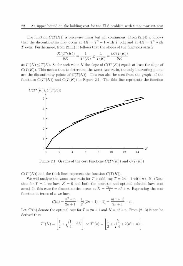
are the discontinuity points of C(T (K)). This can also be seen from the graphs of the

functions C(T ∗(K)) and C(T (K)) in Figure 2.1. The thin line represents the function

0

1

2

3

4

5

0 2 4 6 8 10 12 14

C(T ∗(K)), C(T (K))

K

6

-

Figure 2.1: Graphs of the cost functions C(T ∗(K)) and C(T (K))

C(T ∗(K)) and the thick lines represent the function C(T (K)).

We will analyze the worst case ratio for T is odd, say T = 2n + 1 with n ∈ N. (Note

that for T = 1 we have K = 0 and both the heuristic and optimal solution have cost

zero.) In this case the discontinuities occur at K = T 2−14

= n2 + n. Expressing the cost

function in terms of n we have

C(n) =n2 + n

2n + 1+

1

2((2n + 1) − 1) =

n(n + 1)

2n + 1+ n.

Let C∗(n) denote the optimal cost for T = 2n + 1 and K = n2 + n. From (2.13) it can be

derived that

T ∗(K) =

⌊1

2+

√1

4+ 2K

⌋

or T ∗(n) =

⌊1

2+

√1

4+ 2(n2 + n)

⌋

.

33

2.5 Conclusion 23

So we have

C∗(n) =n(n + 1)⌊

12

+√

14

+ 2(n2 + n)⌋ +

1

2

(⌊1

2+

√1

4+ 2(n2 + n)

⌋− 1

).

For odd values of T the worst case ratio can now be expressed in terms of n as

supn∈N

C(n)

C∗(n)

.

For n = 1, 2, 3, 4, . . . we have C(n)C∗(n)

= 109, 16

15, 15

14, 16

15, . . . . It can be shown that C(n)

C∗(n)is

maximal for n = 1. Furthermore, we have

limn→∞

C(n)

n=

3

2and lim

n→∞

C∗(n)

n=

√2,

implying that

limn→∞

C(n)

C∗(n)= lim

n→∞

C(n)/n

C∗(n)/n=

3

4

√2.

For even values of T a similar analysis as above shows that the worst case ratio is smaller

than 1514

and the limiting value is 34

√2. In conclusion, for a given setup cost K the relative

error lies in the interval [0, 19] and the relative error tends to 3

4

√2 − 1 ≤ 6.1% for K

sufficiently large.

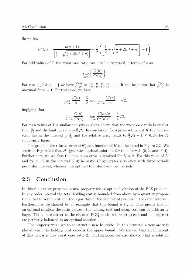
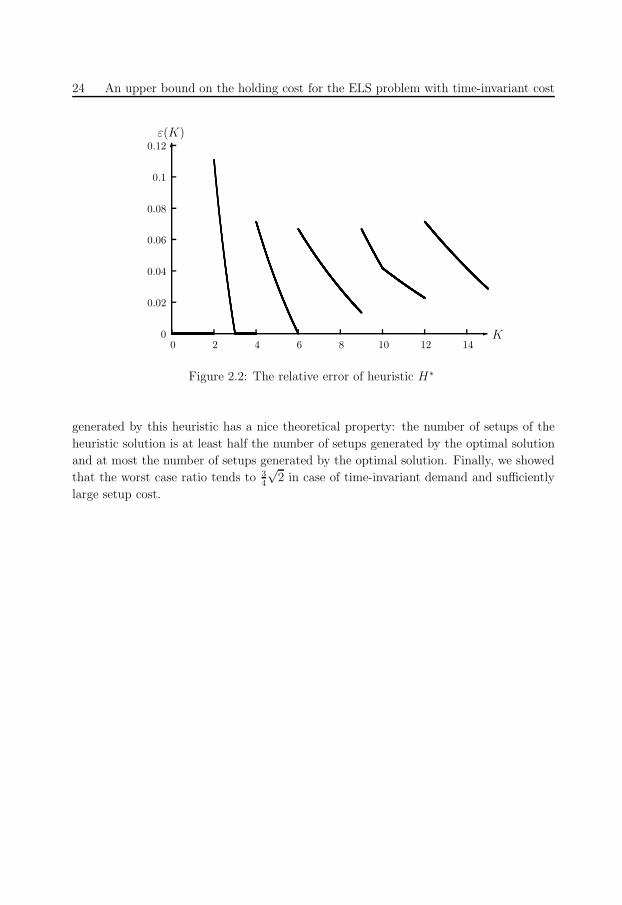
The graph of the relative error ε(K) as a function of K can be found in Figure 2.2. We

see from Figure 2.2 that H∗ generates optimal solutions for the intervals 〈0, 2〉 and [3, 4〉.Furthermore, we see that the maximum error is attained for K = 2. For this value of K

and for all K in the interval [2, 3〉 heuristic H∗ generates a solution with three periods

per order interval, whereas it is optimal to order every two periods.

2.5 Conclusion

In this chapter we presented a new property for an optimal solution of the ELS problem.

In any order interval the total holding cost is bounded from above by a quantity propor-

tional to the setup cost and the logarithm of the number of periods in the order interval.

Furthermore, we showed by an example that this bound is tight. This means that in

an optimal solution the ratio between the holding cost and setup cost can be arbitrarily

large. This is in contrast to the classical EOQ model where setup cost and holding cost

are perfectly balanced in an optimal solution.

The property was used to construct a new heuristic. In this heuristic a new order is

placed when the holding cost exceeds the upper bound. We showed that a refinement

of this heuristic has worst case ratio 2. Furthermore, we also showed that a solution

34

24 An upper bound on the holding cost for the ELS problem with time-invariant cost

0

0.02

0.04

0.06

0.08

0.1

0.12

0 2 4 6 8 10 12 14

ε(K)

K

6

-

Figure 2.2: The relative error of heuristic H∗

generated by this heuristic has a nice theoretical property: the number of setups of the

heuristic solution is at least half the number of setups generated by the optimal solution

and at most the number of setups generated by the optimal solution. Finally, we showed

that the worst case ratio tends to 34

√2 in case of time-invariant demand and sufficiently

large setup cost.

35

Chapter 3

Performance bounds for a general

class of on-line lot-sizing heuristics

Abstract

In this chapter we analyze the worst case performance of heuristics for the classical

economic lot-sizing problem with time-invariant cost parameters. We consider a

general class of on-line heuristics that is often applied in a rolling horizon environ-

ment. We develop procedures to systematically construct worst case instances for

a fixed time horizon and use them to derive worst case problem instances for an

infinite time horizon. Our analysis shows that the heuristics in our class have worst

case ratio at least 2 and a worst case ratio at least 32 if we relax some assump-

tions. Furthermore, we show how the results can be used to construct heuristics

with optimal worst case performance for small model horizons.

3.1 Introduction

The economic lot-sizing (ELS) problem is a well-known problem in inventory management

and is described as follows. Given the (deterministic) demand for a discrete and finite

planning horizon, find a production plan that satisfies demand and minimizes total costs.

Costs include setup cost for each time period production takes place and holding cost for

each item carried over from a period to the next period.

Although the ELS problem can be solved in polynomial time, heuristics are often used

to solve the problem. One reason is that exact algorithms (such as the algorithm by

Wagner and Whitin (1958)) are difficult to understand and hence are often not used by

practitioners. Furthermore, heuristics are often applied when the ELS problem needs to

be solved in a rolling horizon environment. In that situation heuristics may perform better

than the Wagner-Whitin-algorithm (see for example Stadtler (2000) and Van den Heuvel

36

26 Performance bounds for a general class of on-line lot-sizing heuristics

and Wagelmans (2005)). Note that in a rolling horizon environment, lot-sizing heuristics

can be considered as on-line algorithms, because decisions have to be taken while not all

future demand information is known.

Two methods are commonly used to measure the performance of heuristics. First, we

have the empirical methods in which a simulation study is performed (see, e.g., Baker

(1989), Fisher et al. (2001) and Simpson (2001)). The difficulty of a simulation study

is to construct a representative testbed. Second, we have analytical methods which can

be split into probabilistic and worst case analysis. Probabilistic methods analyze the

expected performance of heuristics given the distribution of some problem parameters

(see Axsater (1988)). In worst case analysis one searches for a bound on the relative

performance of heuristics for any problem instance (see Axsater (1982), Bitran et al.

(1984), Axsater (1985) and Vachani (1992)).

In this chapter we are interested in the worst case performance of heuristics for the

ELS problem. As mentioned above several papers on this subject have appeared in the

literature. Axsater (1982) and Bitran et al. (1984) analyze the worst case performance

of some specific lot-sizing rules. Vachani (1992) analyzes the worst case performance of

seven heuristics, where also data dependence, such as the length of the time horizon and

demand properties (constant and bounded demand), is taken into account. The paper

that is closest to our research is Axsater (1985). He shows that all on-line heuristics which

use a specific type of decision rule have worst case ratio at least 2. A nice aspect of this

result is that it applies to almost all popular heuristics.

Our research was motivated by the following natural questions. First, do there exist

on-line heuristics with worst case performance smaller than 2? Second, can we construct

problem instances with large performance ratio for a broader class of on-line heuristics

than Axsater (1985)? In this chapter we will provide a positive answer to the last ques-

tion by showing that a general class of on-line heuristics has worst case ratio at least 2.

Although this means that we generalize the result of Axsater (1985), we would like to

emphasize that our approach is (necessarily) completely different than his. In fact, we

believe that the actual contribution of this chapter lies not only in the fact that we provide

a worst case problem instance, but also in the description of the systematic way in which

we have searched for this instance.

This chapter is organized as follows. In Section 3.2 we formally introduce the economic

lot-sizing problem and we define our class of on-line heuristics by three properties. In

Section 3.3 we show that heuristics satisfying the first property have worst case ratio

at least 32, whereas Section 3.4 shows that the heuristics satisfying all three properties

have worst case ratio at least 2. In Section 3.5 we show how the analysis of Section 3.3

can be used to construct new heuristics for small time horizons with optimal worst case

performance. The chapter is completed with the conclusion in Section 3.6.

37

3.2 Definitions, problem formulation and observations 27

3.2 Definitions, problem formulation and observations

We start this section by describing the ELS problem mathematically. If we use the

following notation

T : model horizon

dt : demand in period t

K : setup cost

h : unit holding cost

xt : production quantity in period t

It : ending inventory in period t,

then the ELS problem can be modeled as

C∗(d, T ) = min∑T

t=1 (Kδ(xt) + hIt)

s.t. It = It−1 − dt + xt t = 1, . . . , T

xt, It ≥ 0 t = 1, . . . , T

I0 = 0,

where

δ(x) =

0 for x = 0

1 for x > 0.

First, note that we may assume w.l.o.g. that K = 1 as the objective function only depends

on the ratio K/h. Furthermore, we may assume w.l.o.g. that h = 1. Namely, defining the

variables x′t = hxt, I ′

t = hIt and d′t = hdt leads to the model

C∗(d′, T ) = min∑T

t=1 (δ(x′t) + I ′

t)

s.t. I ′t = I ′

t−1 − d′t + x′

t t = 1, . . . , T

x′t, I

′t ≥ 0 t = 1, . . . , T

I ′0 = 0.

This shows that, when considering the worst case performance of heuristics, it suffices to

consider only problem instances with K = h = 1. This means that a problem instance

is completely defined by a demand sequence d = d1, . . . , dT . Finally, we may also assume

w.l.o.g. that d1 > 0 since otherwise this period can be ignored.

Let d be a problem instance and let CH(d) be the cost of a solution generated by some

heuristic H on instance d. We define the performance ratio r(d) of H for instance d as

r(d) = CH(d)/C∗(d), where C∗(d) is the optimal cost for this instance. Furthermore, the

worst case ratio of H is defined as

supd∈I

r(d),

38

28 Performance bounds for a general class of on-line lot-sizing heuristics

where I is the set of all problem instances. From the definitions it follows that the

performance ratio is a measure for a particular problem instance d and the worst ratio is

a measure for a set of instances.

Axsater (1985) considers a class of on-line heuristics where a setup is made in period n+

1 (with the previous setup in period 1) if

k∑

t=1

atkdt ≤ 1 for k = 2, . . . , n and

n+1∑

t=1

at,n+1dt > 1,

where atk (1 ≤ t ≤ k ≤ T ) are constants. After the setup assignment to period n + 1,

this period becomes period 1 and the procedure starts again. Axsater (1985) proves that

this class of heuristics has a worst case ratio of at least 2 (and this bound is tight for

some heuristics) by considering nine different cases dependent on the properties of the

constants atk.

As in Axsater (1985) we consider a complete class of on-line heuristics. Our general

class of heuristics is defined by the following properties:

Property 1 Decisions are made period by period (so previously made decisions are fixed

and cannot be changed) and the decision whether to have a setup or not in a period does

not depend on future demand.

Property 2 The decision whether to have a setup or not only depends on the cost of the

current lot-size.

Property 3 The heuristics are deterministic, i.e., applying the heuristic to the same

problem instance leads to the same outcome.

Property 1 states that the decisions are made starting in period 1 and in every next period

we decide whether to make a setup or not irrespective of future demand. Property 2 is a

natural assumption. If period s is a setup period, then the decision in period t > s does

not affect the cost before period s and hence these costs are not taken into account when

making the decision. Property 3 essentially states that the heuristic is consistent. As far

as we know no randomized on-line algorithms are known for the ELS problem. Therefore,

Property 3 does not seem to exclude any heuristic proposed in the literature. It is clear

that the class of Axsater (1985) is contained in the class of heuristics we consider. This

implies that the best worst case ratio of any heuristic in our class is at most 2. The

heuristic we proposed in Chapter 2 is a heuristic with worst case ratio 2 and included in

our class of heuristics but not in the class considered by Axsater (1985).

39

3.2 Definitions, problem formulation and observations 29

Because we are interested in the best heuristics within our class, some heuristics can

immediately be eliminated from the analysis. Assume there is a demand instance with

dt > 1 in some period t > 1 and assume there is some heuristic H that generates no

setup in period t. Let s be the setup period preceding period t. Then the holding cost of

demand in period t equals (t − s)dt > 1. So having a setup in period t is less expensive

and by this additional setup the holding cost for demands after period t will also decrease.

In other words, any heuristics H ′ that generates the same setups as H including setups

in periods with dt > 1 is better than H . Therefore, H can be left out of consideration

when analyzing our class of heuristics.

Using this observation, the Lemma 3.1 shows that only problem instances with dt ≤ 1

are of interest when we are looking for worst case examples. For this reason we will assume

that dt ≤ 1 in the remainder of this chapter.

Lemma 3.1 If there exists a problem instance d = d1, . . . , dT with dt > 1 for some

t > 1 and a heuristic H satisfying Properties 1-3 and having performance ratio r for this

instance, then there also exists a problem instance d′ with d′t ≤ 1 and performance ratio

at least r.

Proof Let t > 1 the smallest period with dt > 1. First, both the optimal solution and

any heuristic H will have a setup in period t and assume that they have cost C∗ and

CH , respectively. Furthermore, let C∗1,t−1 and C∗

t,T (CH1,t−1 and CH

t,T ) be the cost of the

optimal (heuristic) solution for periods 1, . . . , t−1 and periods t, . . . , T , respectively. Now

consider the instances d1 = d1, . . . , dt−1 and d2 = dt, . . . , dT with the modification dt = 1.

Because of the properties of our class of heuristics, H will generate a solution with cost

CH1,t−1 for d1 and a solution with cost CH

t,T for d2. Because

C∗/CH = (CH1,t−1 + CH

t,T )/(C∗1,t−1 + C∗

t,T ) = r ⇔ CH1,t−1 + CH

t,T = rC∗1,t−1 + rC∗

t,T ,

either

CH1,t−1 ≥ rC∗

1,t−1 ⇔ CH1,t−1/C

∗1,t−1 ≥ r,

or

CHt,T ≥ rC∗

t,T ⇔ CHt,T /C∗

t,T ≥ r.

So in one of the cases we have an instance with performance ratio at least r. For instance

d1 we have that demands equal at most 1. If instance d2 has performance ratio at least r

and it has another period with demand strictly larger than 1, then repeating the above

argument will lead to a problem instance with performance ratio at least r and demands

at most 1.

The observation that K = h = 1 w.l.o.g. and that dt ≤ 1 leads to some interesting

insights. First, it is clear that every problem instance has cost at most T : the cost of the

40

30 Performance bounds for a general class of on-line lot-sizing heuristics

trivial lot-for-lot (L4L) heuristic which has a setup in each period. Because the optimal

solution has cost at least 1, the worst case ratio of L4L is at most T . Furthermore, if

dt ≥ p > 0 for all t = 1, . . . , T , then the optimal solution has cost at least p in each

period and the worst case ratio of L4L is at most TTp

= 1p. Now look at Table 3.1

where we reproduced the summary of the worst case analysis on the seven heuristics by

Vachani (1992, p. 805, Table 2). When we look at instances with a finite time horizon

Heuristic T dt = d dt ≤ p, p > 0 dt ≥ p, p ≤ 1

EOQ ∞ 1.059 ∞ ∞POQ T 1.059 ∞ ∞SM

√T/2

√2 ≤ w ≤ T 1 ∞ 1

p

LUC ∞ 1 ∞ ∞PPB 3T/(T + 2) 3

23 3 − 2p

BMY 2T/(T + 1) 1 2 2 − p

FC√

T/2√

2 ≤ w ≤ T ∞ ∞ 1p

Table 3.1: Data dependent worst case ratios (w) of some heuristics

(column 2) and demand bounded from below (column 5), then it follows that in the worst

case only PPB and BMY perform strictly better than the L4L heuristic. The other five

heuristics perform as bad or even worse than the L4L heuristic on one of the two problem

characteristics. So from a worst case analysis point of view these heuristics perform badly.

3.3 Constructing worst case examples for heuristics

satisfying Property 1

In this section we will assume that heuristics satisfy Property 1. So in each period the

heuristic ‘decides’ to start a new order a to add the demand to the current order. By this

property worst case performance can be interpreted as a game between a heuristic and

an adversary. In each period t the heuristic ‘receives’ some demand dt from the adversary

and the heuristic has to ‘decide’ whether to add demand dt to the current production

run (incurring holding cost) or to start a new one (incurring setup cost). Whereas the

heuristic wants to minimize the performance ratio, the adversary tries to maximize the

performance ratio.

41

3.3 Constructing worst case examples for heuristics satisfying Property 1 31

3.3.1 A relaxed mathematical formulation of the problem

It is well known that given a demand sequence d = d1, . . . , dT , a solution for the ELS

problem is completely determined by its setup periods (the zero inventory property). A

production plan (consisting of all setup periods) can be represented by a vector P ∈0, 1T with Pt = 1 if t is a setup period and Pt = 0 otherwise. As we may assume w.l.o.g.

that demand in period 1 is positive, P1 = 1. Let P (T ) be the set of all production plans

of T periods. Let d = d1, . . . , dT be a demand sequence and P ∈ P (T ) a production

plan. Let C(d, P, t) be the cost of the first t periods for demand sequence d in production

plan P , i.e.,

C(d, P, t) =t∑

i=1

(Pi + (i − p(i))dt) , (3.1)

where p(i) is the setup period preceding period i (or period i itself if i is a setup period).

Then the performance ratio for instance d and plan P is defined as

maxt=1,...,T

C(d, P, t)

C∗(d, t).

Note that we take the maximum over all periods as every sequence d1, . . . , dt represents

a problem instance for the ELS problem (the adversary can stop at any moment or the

demand beyond period t can be set equal to zero).

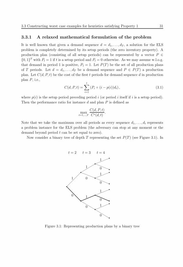
Now consider a binary tree of depth T representing the set P (T ) (see Figure 3.1). In

1

1

1

1

1

1

1

0

0

0

0

0

0

0

t = 2 t = 3 t = 4

Figure 3.1: Representing production plans by a binary tree

42

32 Performance bounds for a general class of on-line lot-sizing heuristics

each node of depth t one branch represents a new setup in period t + 1 and the other

branch represents a non-setup period. For example, the path in Figure 3.1 represents the

plan P = 1, 0, 1, 0. Note that given a demand sequence, every heuristic has to choose

a path (corresponding to a production plan) through the binary tree. So the tree reflects

that decisions are made according to Property 1. Hence the performance ratio R(d, T ) of

any heuristic on demand sequence d of length T equals at least

R∗(d, T ) = minP∈P (T )

maxt=1,...,T

C(d, P, t)

C∗(d, t)

and the worst case ratio of any heuristic equals at least

W ∗(T ) = maxd∈[0,1]T

R∗(d, T ) = maxd∈[0,1]T

minP∈P (T )

maxt=1,...,T

C(d, P, t)

C∗(d, t)(3.2)

as the worst case ratio is the worst performance ratio over all problem instances. Again we

only consider problem instances with demand dt ≤ 1. If we have an instance d with some

demands strictly larger than 1 and if d′ is the instance with demand 1 for these periods,

then it is not difficult to see that R∗(d, T ) = R∗(d′, T ) and hence d can be ignored when

evaluating (3.2). (Note that Lemma 3.1 cannot be applied because Properties 2 and 3 do

not hold.)

The above formulation is not complete. This can be seen as follows. Assume that we

have two demand sequences d1 = [d1, d2, d13] and d2 = [d1, d2, d

23]. Furthermore, assume

that the performance ratios for each (partial) production plan are as shown in Figure 3.2,

where (as in Figure 3.1) an upper branch represents a setup period. It follows from

1 1

32

1

1

132

32

2

2

32

1

d1 d2

2

2

Figure 3.2: Performance ratio for d1 and d2

the figure that R∗(d1, 3) = R∗(d2, 3) = 32. If d1 and d2 are the only possible problem

instances, then from (3.2) it follows W ∗(3) = 32. However, the worst case performance of

any heuristic H is at least 2. Namely, if H generates no setup in period 2, then we give

d13 in period 3 leading to performance ratio 2. On the other hand, if H generates a setup

in period 2, then we give d23 in period 3 again leading to performance ratio 2. Hence the

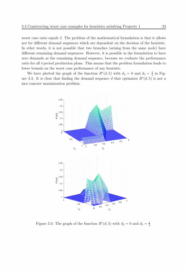
43

3.3 Constructing worst case examples for heuristics satisfying Property 1 33

worst case ratio equals 2. The problem of the mathematical formulation is that it allows

not for different demand sequences which are dependent on the decision of the heuristic.

In other words, it is not possible that two branches (arising from the same node) have

different remaining demand sequences. However, it is possible in the formulation to have

zero demands as the remaining demand sequence, because we evaluate the performance

ratio for all t-period production plans. This means that the problem formulation leads to

lower bounds on the worst case performance of any heuristic.

We have plotted the graph of the function R∗(d, 5) with d2 = 0 and d5 = 14

in Fig-

ure 3.3. It is clear that finding the demand sequence d that optimizes R∗(d, 5) is not a

nice concave maximization problem.

00.2

0.40.6

0.81

0

0.5

1

1

1.05

1.1

1.15

1.2

1.25

d3d

4

R* (d

,5)

00.2

0.40.6

0.81

0

0.5

1

1

1.05

1.1

1.15

1.2

1.25

d3

d4

R* (d

,5)

Figure 3.3: The graph of the function R∗(d, 5) with d2 = 0 and d5 = 14

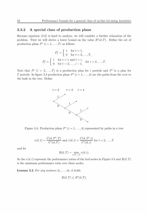
44

34 Performance bounds for a general class of on-line lot-sizing heuristics

3.3.2 A special class of production plans

Because equation (3.2) is hard to analyze, we will consider a further relaxation of the

problem. First we will derive a lower bound on the value R∗(d, T ). Define the set of

production plans P i (i = 1, . . . , T ) as follows

P 1t =

1 for t = 1,

0 for t = 2, . . . , T,

P it =

1 for t = 1 and t = i,

0 for t = 2, . . . , i − 1,for i = 2, . . . , T.

Note that P i (i = 2, . . . , T ) is a production plan for i periods and P 1 is a plan for

T periods. In figure 3.4 production plans P i (i = 1, . . . , 4) are the paths from the root to

the leafs in the tree. Define

1

0

t = 2 t = 3 t = 4

1

10

0

Figure 3.4: Production plans P i (i = 1, . . . , 4) represented by paths in a tree

r(d, 1) =C(d, P 1, T )

C∗(d, T )and r(d, i) =

C(d, P i, i)

C∗(d, i)for i = 2, . . . , T

and let

R(d, T ) = mini=1,...,T

r(d, i).

So the r(d, i) represent the performance ratios of the leaf nodes in Figure 3.4 and R(d, T )

is the minimum performance ratio over these nodes.

Lemma 3.2 For any instance d1, . . . , dT it holds

R(d, T ) ≤ R∗(d, T ).

45

3.3 Constructing worst case examples for heuristics satisfying Property 1 35

Proof Let P ∈ P (T ). Then there exists a j for which P j is a subpath of P . But then

r(d, j) ≤ maxi=1,...,T

C(d, P, i)

C∗(d, i)

as the term at the left hand side is contained in the maximum at the right hand side.

Lemma 3.2 shows that, when using the special set of production plans, we have a lower

bound on the performance ratio for d. The motivation for taking P i (i = 2, . . . , T ) is

that one expects that these plans lead to high costs because in general it is not profitable

to have a setup in the last period. Plan P 1 is needed, because with this plan included,

any production plan P has a plan P i as subplan (and so without P 1 Lemma 3.2 does

not hold). It is clear that for a fixed d the value R(d, T ) is a lower bound on W ∗(T ).

Furthermore, we define the lower bound W (T ) on W ∗(T ) as

W (T ) = maxd∈[0,1]T

R(d, T ) = maxd∈[0,1]T

mint=1,...,T

r(d, t). (3.3)

Note that problem (3.3) is more tractable then problem (3.2) because the ‘min max’-part

is replaced by a ‘min’-part. We will now derive some properties for a demand sequence

that maximizes (3.3).

Lemma 3.3 Let d be an instance that maximizes (3.3). Then the value of dT = 1T−1

.

Proof First note that dT only occurs in the calculation of r(d, 1) and r(d, T ) because they

contain the terms C(d, P 1, T ) and C∗(d, T ). The holding costs for dT equal (T − 1)dT

in plan P 1. If p ≥ 2 is the setup period preceding period T in the optimal plan P ∗,

then the holding cost in this plan equals (T − p)dT (if p = 1, then r(d, 1) = 1 and hence

W (T ) = 1, which cannot optimal). Increasing dT will increase the performance ratio

r(d, 1) = C(d,P 1,T )C∗(d,T )

. However, the performance ratio r(d, T ) = C(d,P T ,T )C∗(d,T )

is decreasing in dT .

Therefore, min r(d, 1), r(d, T ) is maximized when C(d, P 1, T ) = C(d, P T , T ), i.e., when

(T − 1)dT = 1 or dT = 1T−1

.

In the remainder of this chapter we will assume that dT = 1T−1

so that r(d, 1) = r(d, T )

and hence

W (T ) = maxd∈[0,1]T

mini=2,...,T

r(d, i). (3.4)

Another useful property of an optimal demand sequence can be found in the following

lemma.

Lemma 3.4 Let d be an instance with dj−1 > 0, dj = 0 and 3 ≤ j ≤ T . Then there

exists an instance d′ with R(d′, T ) ≥ R(d, T ) and d′j > 0.

46

36 Performance bounds for a general class of on-line lot-sizing heuristics

Proof Define an instance d′ with d′2 = 0 and d′

t+1 = t−1t

dt for all t < j and d′t = dt

for all t > j. So demand before period j is shifted one period and scaled. Clearly,

d′j = j−2

j−1dj−1 > 0. Let i ≤ j. Then the holding cost for demand d′

t+1 (t < i) in P i+1

equals td′t+1 = t t−1

tdt = (t−1)dt, which is the holding cost for demand dt in P i. Therefore,

C(d′, P i+1, i + 1) = C(d, P i, i) for i ≤ j. Furthermore, because demand beyond period j

is unchanged we also have C(d′, P i, i) = C(d, P i, i) for i > j.

Let P be the optimal plan for some i-period problem for instance d. Now shift all

setup periods before period j (except for period 1) one period further. We will use

this plan for the (i + 1)-period problem with demand d′ if i < j and for the i-period

problem with demand d′ if i > j. Clearly, the setup costs for both plans are equal.

Furthermore, let t < j and let p be the setup period before period t in plan P . Then the

holding cost for demand dt equals (t − p)dt and the holding cost for demand d′t+1 equals

((t + 1) − (p + 1))d′t = (t − p) t−1

tdt ≤ (t − p + 1)dt. Using similar arguments one can

show that holding cost for d′t equals at most the holding cost for dt for t > j. Therefore,

C∗(d, i) ≥ C∗(d′, i + 1) for i < j and C∗(d, i) ≥ C∗(d′, i) for i > j.

Using the above (in)equalities it follows that

r(d, i) = C(d,P i,i)C∗(d,i)

≤ C(d′,P i+1,i+1)C∗(d′,i+1)

= r(d′, i + 1) for i < j

r(d, i) = C(d,P i,i)C∗(d,i)

≤ C(d′,P i,i)C∗(d′,i)

= r(d′, i) for i > j.

Furthermore, r(d, j) ≥ r(d, j − 1) because C(d, P j, j) ≥ C(d, P j−1, j − 1) and C∗(d, j) =

C∗(d, j − 1) since dj = 0. Now the lemma follows because

R(d, T ) = mini=2,...,T

r(d, i) ≤ mini=2,...,T

r(d′, i) = R(d′, T ).

The previous lemma shows that if we have an instance with a positive demand period

followed by a zero demand period, then we can find an instance with larger performance

ratio by shifting and scaling all the demand before this zero demand period by one period.

Therefore, there exists a solution that maximizes (3.4) and has no positive demands

followed by zero demands (except for period 1). Let d be a problem instance with dt = 0

for t = 2, . . . , n − 1. For this instance we have r(d, i) = 2 for i = 2, . . . , n − 1 and hence

R(d, T ) is equal to

R(d, T ) = mini=n,...,T

r(d, i).

Let W (T, n) be the maximum of (3.4) with dt = 0 for t = 2, . . . , n − 1, i.e.,

W (T, n) = maxdt∈[0,1],t=n,...,T−1

mini=n,...,T

r(d, i). (3.5)

Then the following corollaries follow immediately from Lemma 3.4.

47

3.3 Constructing worst case examples for heuristics satisfying Property 1 37

Corollary 3.5 For any model horizon T it holds

W (T ) = max1<n<T

W (T, n). (3.6)

Corollary 3.6 For 1 < n < T we have W (T, n) ≤ W (T + 1, n + 1).

Proof A T -period instance can be considered as a (T +1)-period instance with dT+1 = 0.

The following lemma shows another property of an optimal demand sequence.

Lemma 3.7 Let d∗ be an optimal solution of (3.5) with n > 1 the first period with dn > 0

and dt > 0 for t = n, . . . , T . Then r(d∗, i) = r(d∗, i + 1) for i = n, . . . , T − 1.

Proof Assume that the lemma does not hold and let

r(d∗, u) = mini=n,...,T

r(d∗, i) < maxi=n,...,T

r(d∗, i) = r(d, v).

Assume that u < v (the case with u > v can be proven analogously). We will construct

an alternative solution with demand sequence d′ = d∗ + ε such that r(d∗, u) < r(d′, u) ≤r(d′, v) and r(d′, i) = r(d∗, i) for i ∈ n, . . . , T\u, v. This means we have found a

better solution for (3.5) which is a contradiction.

To achieve this, let ri = r(d∗, i) for i = n, . . . , T , keep the production plans fixed and

consider the equations r(d, i) = ri in the variables dn, . . . , dT−1. So the function r(d, i)

is the ratio of two linear functions (see equation (3.1)), r(d, i) is defined on the variables

dn, . . . , di for i = n, . . . , T − 1 and r(d, T ) is defined on the variables dn, . . . , dT−1. First,

note that the optimal plan P ∗i will not have a setup in period i, because moving the setup

from period i to period i− 1 will not increase the cost. Therefore, r(d, i) is either strictly

increasing or strictly decreasing in di, because di appears in the denominator and it does

not appear in the nominator. Similarly, r(d, T ) is either strictly increasing or strictly

decreasing in dT−1, because dT−1 appears in the nominator.

Now let d′i = d∗

i for i = n, . . . , u − 1 and let d′u = d∗

u + εu with εu ∈ R such that

r(d′, u) > r(d∗, u). Note that r(d′, i) = ri for i = n, . . . , u − 1 and r(d′, i) may be

changed for i = u, . . . , T . Now choose εi with d′i = d∗

i + εi such that r(d′, i) = ri for

i = u + 1, . . . , v − 1. Because the function r(d, i) is strictly in/decreasing in di, the value

d′i = d∗

i + εi is uniquely defined by the equation r(d′, i) = ri for given d′n, . . . , d

′i−1 and

hence the values εi (i = u + 1, . . . , v − 1) exist. In a similar way we choose d′i = d∗

i + εi

for i = v, . . . , T − 1 such that r(d′, i) = ri for i = v + 1, . . . , T . Again such values

εi (i = v, . . . , T − 1) exist. Namely, start with an arbitrary value of εv. Then the

values εi (i = v + 1, . . . , T − 1) are uniquely determined by the equations r(d′, i) = ri for

i = v+1, . . . , T −1. Now it is possible that r(d′, T ) 6= rT . This means that the choice of εv

48

38 Performance bounds for a general class of on-line lot-sizing heuristics

was not right and the right value of εv can be found by binary search since r(d, i) is strictly

in/decreasing in di. So summarizing, given an εu, the values εi for i = u + 1, . . . , T − 1

are uniquely determined by the equations r(d′, i) = ri for i ∈ u + 1, . . . , T\v.Finally, consider the value r(d′, v). If r(d′, v) ≥ r(d∗, v), then we have proved the

lemma as we have found a strictly better solution for (3.5) which is a contradiction. If

r(d′, v) < r(d∗, v), then we choose εu sufficiently small such that r(d′, v) ≥ r(d′, u) >

r(d∗, u) and again we have found a better solution.

We end the proof with some remarks. First, if period u is not unique, then we can

repeat the above procedure. Second, if there is some d′i < 0 (which is not feasible), then εu

must be chosen sufficiently small such that d′i ≥ 0. Third, it is possible that by the change

from d∗ to d′ the optimal production plans will also change. In this case the denominator

of r(d′, i) will be smaller and hence r(d′, i) will be larger which means that the proof still

holds.

3.3.3 Finding the optimal demand sequence given the produc-

tion plans

If we can find the values W (T, n), then by Corollary 3.5 we can find the value W (T ).

The difficulty in evaluating W (T, n) is that the optimal plans and the optimal demand

sequences have to be determined simultaneously. For example, a change in a demand

sequence may cause a change in the optimal production plans. In this section we will

derive an approach to calculate the optimal demand sequence assuming that the optimal

production plans are known.

Assume that we have a demand sequence with dt = 0 for t = 2, . . . , n − 1. If the

optimal plans are known, then by Lemma 3.7 the optimal demand sequence (with respect

to (3.5)) can be found by solving the system

r(d, i) = r(d, i + 1) for i = n, . . . , T − 1. (3.7)

Given the plans P i (i = n, . . . , T ) and the optimal production plans P ∗i for each hori-

zon i = n, . . . , T , it follows from (3.1) that both the nominator and the denominator

of r(d, i) = C(d,P i,i)C(d,P ∗i,i)

are linear functions in the variables dn, . . . , dT−1. Now by ‘cross-

multiplying’, system (3.7) is a system of multivariate quadratic equations. This is in

general a hard problem, because by the method of repeated substitution one has to find

the roots of univariate polynomials of high degree. Example 3.8 illustrates this.

Example 3.8 Consider a problem with T = 5 and n = 3 so that d2 = 0 and d5 = 14. In

Table 3.2 the production plans, corresponding costs and performance ratios are shown.

From r(d, 3) = r(d, 4) it follows that d4 = 2d23 + 3d3 − 1. Substituting this in r(d, 3) =

r(d, 5) we have 12d33 + 24d2

3 + 3d3 − 4 = 0. Solving this equation we have d∗3 ≈ 0.328,

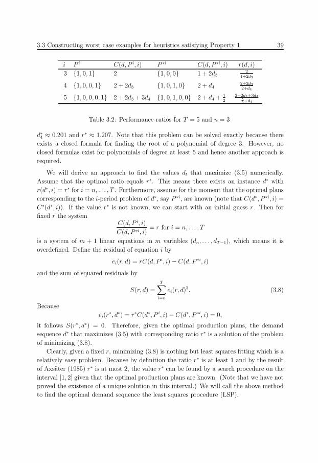
49

3.3 Constructing worst case examples for heuristics satisfying Property 1 39

i P i C(d, P i, i) P ∗i C(d, P ∗i, i) r(d, i)

3 1, 0, 1 2 1, 0, 0 1 + 2d32

1+2d3

4 1, 0, 0, 1 2 + 2d3 1, 0, 1, 0 2 + d42+2d3

2+d4

5 1, 0, 0, 0, 1 2 + 2d3 + 3d4 1, 0, 1, 0, 0 2 + d4 + 12

2+2d3+3d45

2+d4

Table 3.2: Performance ratios for T = 5 and n = 3

d∗4 ≈ 0.201 and r∗ ≈ 1.207. Note that this problem can be solved exactly because there

exists a closed formula for finding the root of a polynomial of degree 3. However, no

closed formulas exist for polynomials of degree at least 5 and hence another approach is

required.

We will derive an approach to find the values dt that maximize (3.5) numerically.

Assume that the optimal ratio equals r∗. This means there exists an instance d∗ with

r(d∗, i) = r∗ for i = n, . . . , T . Furthermore, assume for the moment that the optimal plans

corresponding to the i-period problem of d∗, say P ∗i, are known (note that C(d∗, P ∗i, i) =

C∗(d∗, i)). If the value r∗ is not known, we can start with an initial guess r. Then for

fixed r the systemC(d, P i, i)

C(d, P ∗i, i)= r for i = n, . . . , T

is a system of m + 1 linear equations in m variables (dn, . . . , dT−1), which means it is

overdefined. Define the residual of equation i by

ei(r, d) = rC(d, P i, i) − C(d, P ∗i, i)

and the sum of squared residuals by

S(r, d) =T∑

i=n

ei(r, d)2. (3.8)

Because

ei(r∗, d∗) = r∗C(d∗, P i, i) − C(d∗, P ∗i, i) = 0,

it follows S(r∗, d∗) = 0. Therefore, given the optimal production plans, the demand

sequence d∗ that maximizes (3.5) with corresponding ratio r∗ is a solution of the problem

of minimizing (3.8).

Clearly, given a fixed r, minimizing (3.8) is nothing but least squares fitting which is a

relatively easy problem. Because by definition the ratio r∗ is at least 1 and by the result

of Axsater (1985) r∗ is at most 2, the value r∗ can be found by a search procedure on the

interval [1, 2] given that the optimal production plans are known. (Note that we have not

proved the existence of a unique solution in this interval.) We will call the above method

to find the optimal demand sequence the least squares procedure (LSP).

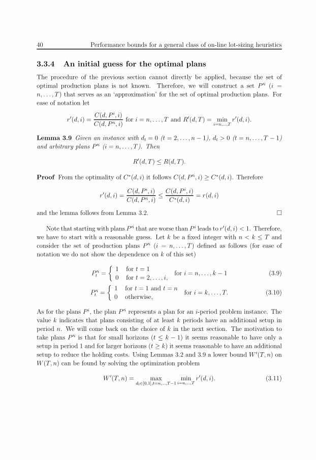
50

40 Performance bounds for a general class of on-line lot-sizing heuristics

3.3.4 An initial guess for the optimal plans

The procedure of the previous section cannot directly be applied, because the set of

optimal production plans is not known. Therefore, we will construct a set P ′i (i =

n, . . . , T ) that serves as an ‘approximation’ for the set of optimal production plans. For

ease of notation let

r′(d, i) =C(d, P i, i)

C(d, P ′i, i)for i = n, . . . , T and R′(d, T ) = min

i=n,...,Tr′(d, i).

Lemma 3.9 Given an instance with dt = 0 (t = 2, . . . , n − 1), dt > 0 (t = n, . . . , T − 1)

and arbitrary plans P ′i (i = n, . . . , T ). Then

R′(d, T ) ≤ R(d, T ).

Proof From the optimality of C∗(d, i) it follows C(d, P ′i, i) ≥ C∗(d, i). Therefore

r′(d, i) =C(d, P i, i)

C(d, P ′i, i)≤ C(d, P i, i)

C∗(d, i)= r(d, i)

and the lemma follows from Lemma 3.2.

Note that starting with plans P ′i that are worse than P i leads to r′(d, i) < 1. Therefore,

we have to start with a reasonable guess. Let k be a fixed integer with n < k ≤ T and

consider the set of production plans P ′i (i = n, . . . , T ) defined as follows (for ease of

notation we do not show the dependence on k of this set)

P ′it =

1 for t = 1

0 for t = 2, . . . , i,for i = n, . . . , k − 1 (3.9)

P ′it =

1 for t = 1 and t = n

0 otherwise,for i = k, . . . , T. (3.10)

As for the plans P i, the plan P ′i represents a plan for an i-period problem instance. The

value k indicates that plans consisting of at least k periods have an additional setup in

period n. We will come back on the choice of k in the next section. The motivation to

take plans P ′i is that for small horizons (t ≤ k − 1) it seems reasonable to have only a

setup in period 1 and for larger horizons (t ≥ k) it seems reasonable to have an additional

setup to reduce the holding costs. Using Lemmas 3.2 and 3.9 a lower bound W ′(T, n) on

W (T, n) can be found by solving the optimization problem

W ′(T, n) = maxdt∈[0,1],t=n,...,T−1

mini=n,...,T

r′(d, i). (3.11)

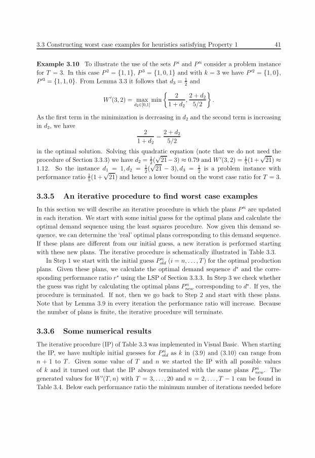
51

3.3 Constructing worst case examples for heuristics satisfying Property 1 41

Example 3.10 To illustrate the use of the sets P i and P ′i consider a problem instance

for T = 3. In this case P 2 = 1, 1, P 3 = 1, 0, 1 and with k = 3 we have P ′2 = 1, 0,P ′3 = 1, 1, 0. From Lemma 3.3 it follows that d3 = 1

2and

W ′(3, 2) = maxd2∈[0,1]

min

2

1 + d2,2 + d2

5/2

.

As the first term in the minimization is decreasing in d2 and the second term is increasing

in d2, we have2

1 + d2

=2 + d2

5/2

in the optimal solution. Solving this quadratic equation (note that we do not need the

procedure of Section 3.3.3) we have d2 = 12(√

21−3) ≈ 0.79 and W ′(3, 2) = 15(1+

√21) ≈

1.12. So the instance d1 = 1, d2 = 12(√

21 − 3), d3 = 12

is a problem instance with

performance ratio 15(1+

√21) and hence a lower bound on the worst case ratio for T = 3.

3.3.5 An iterative procedure to find worst case examples

In this section we will describe an iterative procedure in which the plans P ′i are updated

in each iteration. We start with some initial guess for the optimal plans and calculate the

optimal demand sequence using the least squares procedure. Now given this demand se-

quence, we can determine the ‘real’ optimal plans corresponding to this demand sequence.

If these plans are different from our initial guess, a new iteration is performed starting

with these new plans. The iterative procedure is schematically illustrated in Table 3.3.

In Step 1 we start with the initial guess P ′iold (i = n, . . . , T ) for the optimal production

plans. Given these plans, we calculate the optimal demand sequence d∗ and the corre-

sponding performance ratio r∗ using the LSP of Section 3.3.3. In Step 3 we check whether

the guess was right by calculating the optimal plans P ′inew corresponding to d∗. If yes, the

procedure is terminated. If not, then we go back to Step 2 and start with these plans.

Note that by Lemma 3.9 in every iteration the performance ratio will increase. Because

the number of plans is finite, the iterative procedure will terminate.

3.3.6 Some numerical results

The iterative procedure (IP) of Table 3.3 was implemented in Visual Basic. When starting

the IP, we have multiple initial guesses for P ′iold as k in (3.9) and (3.10) can range from

n + 1 to T . Given some value of T and n we started the IP with all possible values

of k and it turned out that the IP always terminated with the same plans P ′inew. The

generated values for W ′(T, n) with T = 3, . . . , 20 and n = 2, . . . , T − 1 can be found in

Table 3.4. Below each performance ratio the minimum number of iterations needed before

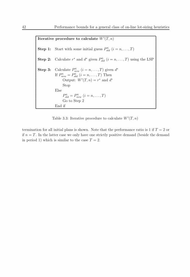
52

42 Performance bounds for a general class of on-line lot-sizing heuristics

Iterative procedure to calculate W ′(T, n)

Step 1: Start with some initial guess P ′iold (i = n, . . . , T )

Step 2: Calculate r∗ and d∗ given P ′iold (i = n, . . . , T ) using the LSP

Step 3: Calculate P ′inew (i = n, . . . , T ) given d∗

If P ′inew = P ′i

old (i = n, . . . , T ) Then

Output: W ′(T, n) = r∗ and d∗

Stop

Else

P ′iold = P ′i

new (i = n, . . . , T )

Go to Step 2

End if

Table 3.3: Iterative procedure to calculate W ′(T, n)

termination for all initial plans is shown. Note that the performance ratio is 1 if T = 2 or

if n = T . In the latter case we only have one strictly positive demand (beside the demand

in period 1) which is similar to the case T = 2.

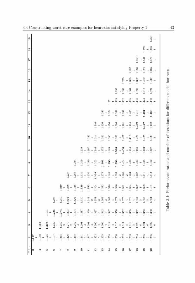
53

3.3 Constructing worst case examples for heuristics satisfying Property 1 43T

\n

23

45

67

89

10

11

12

13

14

15

16

17

18

19

31.117

1

41.1

50

1.165

11

51.1

75

1.207

1.1

91

21

1

61.1

97

1.2

32

1.235

1.2

07

31

11

71.2

15

1.2

52

1.274

1.2

59

1.2

19

43

11

1

81.2

26

1.2

70

1.2

93

1.301

1.2

76

1.2

27

42

11

11

91.2

35

1.2

82

1.3

04

1.320

1.3

18

1.2

89

1.2

34

34

21

11

1

10

1.2

41

1.2

91

1.3

17

1.3

30

1.336

1.3

31

1.2

99

1.2

39

54

31

11

11

11

1.2

47

1.2

98

1.3

29

1.3

43

1.353

1.3

50

1.3

40

1.3

07

1.2

43

44

32

11

11

1

12

1.2

52

1.3

05

1.3

37

1.3

54

1.3

64

1.369

1.3

63

1.3

46

1.3

14

1.2

46

54

33

11

11

11

13

1.2

55

1.3

09

1.3

42

1.3

62

1.3

72

1.3

79

1.381

1.3

72

1.3

52

1.3

20

1.2

49

54

33

21

11

11

1

14

1.2

58

1.3

12

1.3

47

1.3

67

1.3

78

1.3

85

1.390

1.3

89

1.3

80

1.3

56

1.3

24

1.2

51

54

44

21

11

11

11

15

1.2

60

1.3

15

1.3

50

1.3

72

1.3

86

1.3

93

1.398

1.398

1.3

96

1.3

86

1.3

59

1.3

29

1.2

53

45

43

32

11

11

11

1

16

1.2

62

1.3

17

1.3

52

1.3

75

1.3

91

1.4

00

1.4

04

1.408

1.4

07

1.4

01

1.3

91

1.3

62

1.3

32

1.2

55

55

64

32

11

11

11

11

17

1.2

63

1.3

19

1.3

55

1.3

79

1.3

94

1.4

04

1.4

10

1.4

14

1.416

1.4

14

1.4

05

1.3

95

1.3

64

1.3

35

1.2

57

55

54

43

21

11

11

11

1

18

1.2

64

1.3

20

1.3

57

1.3

81

1.3

97

1.4

07

1.4

14

1.4

18

1.4

21

1.422

1.4

19

1.4

08

1.3

99

1.3

67

1.3

38

1.2

58

56

55

43

21

11

11

11

11

19

1.2

65

1.3

21

1.3

58

1.3

83

1.3

99

1.4

11

1.4

18

1.4

23

1.4

25

1.427

1.427

1.4

24

1.4

13

1.4

02

1.3

71

1.3

41

1.2

59

56

55

44

32

11

11

11

11

1

20

1.2

66

1.3

22

1.3

60

1.3

84

1.4

01

1.4

13

1.4

22

1.4

27

1.4

30

1.4

32

1.433

1.4

30

1.4

27

1.4

17

1.4

05

1.3

74

1.3

43

1.2

60

56

54

44

32

21

11

11

11

11

Tab

le3.

4:Per

form

ance

rati

osan

dnum

ber

ofit

erat

ions

for

diff

eren

tm

odel

hor

izon

s

54

44 Performance bounds for a general class of on-line lot-sizing heuristics

Table 3.4 shows some interesting results. First, it follows that W ′(T, n) ≤ W ′(T +

1, n+1). As this property holds for W (T, n) (see Lemma 3.4) and because the IP converges

to the same solutions when starting with different initial guesses, it suggests that W (T, n)

and W ′(T, n) are equal. Second, we see that for a fixed T the value of n that maximizes

W ′(T, n) (the performance ratios in bold), say n(T ), is increasing in T . Furthermore,

we see that for n < n(T ), W ′(T, n) is increasing in n, and for n > n(T ), W ′(T, n) is

decreasing in n. Third, the minimum number of iterations shows that the initial guesses

are reasonable. For n close to T we see that one of the initial guesses is the optimal one.

Finally, we note that for large values of T we can find performance ratios close to 32. For

example, W ′(80, 100) = 1.494 and W ′(480, 500) = 1.499.

Again look at the graph of R∗(d, 5) in Figure 3.3. The function R∗(d, 5) has two local

optima: d13 ≈ 0.328, d1

4 ≈ 0.201 with R∗(d1, 5) ≈ 1.207 and d23 = 0, d2

4 ≈ 0.226 with

R∗(d2, 5) ≈ 1.191. The performance ratios of these two solutions are equal to the ratios

found by the IP (W ′(5, 3) and W ′(5, 4) in Table 3.4), which shows that the IP leads to

the optimal solutions for T = 5 with d2 = 0.

3.3.7 Two convergence results

In this section we will give two convergence results. First, we will give a lower bound on

the worst case ratio of heuristics applied to instances with only positive demands in the

last two periods (and in period 1). Then we will give a problem instance for which any

heuristic satisfying Property 1 has worst case ratio at least 32.

Lemma 3.11 For the value W (T + 1, T ) it holds

limT→∞

W (T + 1, T ) =1

4(√

17 + 1) ≈ 1.281.

Proof Assume that demand in period T equals dT = cT−1

(for ease of notation we use T−1

in the denominator). Furthermore, by Lemma 3.3 we have dT+1 = 1T. It is not difficult

to see that in the T -period problem it is optimal to have a setup only in period 1 for

appropriate c, whereas plan P T has setups in periods 1 and T . So we have r(c, T ) = 21+c

.

For the (T + 1)-period problem it is optimal to have setups in periods 1 and T , whereas

P T+1 has setups in periods 1 and T + 1 implying that

r(c, T + 1) =2 + c

2 + 1T

.

Now the maximum of

W (T + 1, T ) = maxc

min

2

1 + c,

2 + c

2 + 1T

,

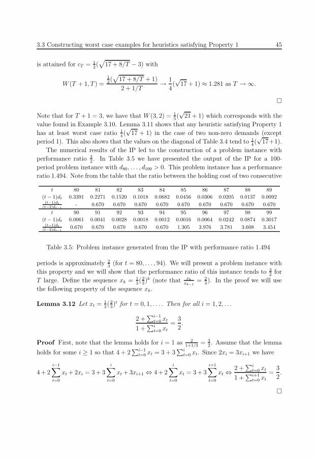
55

3.3 Constructing worst case examples for heuristics satisfying Property 1 45

is attained for cT = 12(√

17 + 8/T − 3) with

W (T + 1, T ) =12(√

17 + 8/T + 1)

2 + 1/T→ 1

4(√

17 + 1) ≈ 1.281 as T → ∞.

Note that for T + 1 = 3, we have that W (3, 2) = 15(√

21 + 1) which corresponds with the

value found in Example 3.10. Lemma 3.11 shows that any heuristic satisfying Property 1

has at least worst case ratio 14(√

17 + 1) in the case of two non-zero demands (except

period 1). This also shows that the values on the diagonal of Table 3.4 tend to 14(√

17+1).

The numerical results of the IP led to the construction of a problem instance with

performance ratio 32. In Table 3.5 we have presented the output of the IP for a 100-

period problem instance with d80, . . . , d100 > 0. This problem instance has a performance

ratio 1.494. Note from the table that the ratio between the holding cost of two consecutive

t 80 81 82 83 84 85 86 87 88 89

(t − 1)dt 0.3391 0.2271 0.1520 0.1018 0.0682 0.0456 0.0306 0.0205 0.0137 0.0092(t−1)dt

(t−2)dt−1

- 0.670 0.670 0.670 0.670 0.670 0.670 0.670 0.670 0.670

t 90 91 92 93 94 95 96 97 98 99

(t − 1)dt 0.0061 0.0041 0.0028 0.0018 0.0012 0.0016 0.0064 0.0242 0.0874 0.3017(t−1)dt

(t−2)dt−1

0.670 0.670 0.670 0.670 0.670 1.305 3.976 3.781 3.608 3.454

Table 3.5: Problem instance generated from the IP with performance ratio 1.494

periods is approximately 23

(for t = 80, . . . , 94). We will present a problem instance with

this property and we will show that the performance ratio of this instance tends to 32

for

T large. Define the sequence xk = 13(2

3)k (note that xk

xk−1= 2

3). In the proof we will use

the following property of the sequence xk.

Lemma 3.12 Let xt = 13(2

3)t for t = 0, 1, . . . . Then for all i = 1, 2, . . .

2 +∑i−1

t=0 xt

1 +∑i

t=0 xt

=3

2.

Proof First, note that the lemma holds for i = 1 as 21+1/3

= 32. Assume that the lemma

holds for some i ≥ 1 so that 4 + 2∑i−1

t=0 xt = 3 + 3∑i

t=0 xt. Since 2xi = 3xi+1 we have

4 + 2

i−1∑

t=0

xt + 2xi = 3 + 3

i∑

t=0

xt + 3xi+1 ⇔ 4 + 2

i∑

t=0

xt = 3 + 3

i+1∑

t=0

xt ⇔2 +

∑it=0 xt

1 +∑i+1

t=0 xt

=3

2.

56

46 Performance bounds for a general class of on-line lot-sizing heuristics

Theorem 3.13 Any heuristic satisfying Property 1 has worst case ratio at least 32.

Proof We will prove the theorem by showing that there exists a problem instance d with

limT→∞

R′(d, T ) =3

2.

Define the demand sequence d with time horizon T 2 + T + 1 as follows: d1 = 1, dt = 0

for t = 2, . . . , T 2 − 1), dt =x

t−T2

t−1for t = T 2, . . . , T 2 + T with xt as in Lemma 3.12 and

dT 2+T+1 = 1T 2+T

. (Using the notation of the previous sections we have set T to T 2 +T +1

and n to T 2.) First, for i = T 2, . . . , T 2 + T + 1 we have

C(d, P i, i) = 2 +

i−1∑

t=T 2

(t − 1)dt = 2 +

i−T 2−1∑

t=0

xt

and

C(d, P 1, T 2 + T + 1) = 1 +

T 2+T+1∑

t=T 2

(t − 1)dt = 1 +

T∑

t=0

xt + 1.

Now let P ′i be a production plan for the i-period problem (i = T 2, . . . , T 2 + T ) with only

a setup in period 1 and let P ′T 2+T+1 be a production plan with setups in periods 1 and T 2

(so using the notation of Section 3.3.4 we have set k to T 2 + T + 1). Then we have

C(d, P ′i, i) = 1 +

i∑

t=T 2

(t − 1)dt = 1 +

i−T 2∑

t=0

x0

and

C(d, P ′T 2+T+1, T 2 + T + 1) = 2 +

T 2+T+1∑

t=T 2+1

(t − T 2)dt = 2 +

T 2+T∑

t=T 2+1

t − T 2

t − 1xt−T 2 +

T + 1

T 2 + T

≤ 2 +T 2+T∑

t=T 2+1

T

T 2xt−T 2 +

1

T= 2 +

1

T

T∑

t=1

1

3

(2

3

)t

+1

T≤ 2 +

2

T.

By Lemma 3.12 we have that

r′(d, i) =2 +

∑i−T 2−1t=0 xt

1 +∑i−T 2

t=0 xt

=3

2for i = T 2, . . . , T 2 + T.

Furthermore, because limT→∞

∑Tt=0 xt = 1 we have that C(d, P T 2+T+1, T 2 + T + 1) → 3,

C(d, P 1, T 2+T+1) → 3 and C(d, P ′T 2+T+1) → 2 as T → ∞ and hence r′(d, T 2+T+1) → 32

and r′(d, 1) → 32

as T → ∞. In conclusion, demand sequence d is an instance with

performance ratio R′(d, T 2 + T + 1) = 32

for T → ∞.

57

3.4 Analysis of heuristics satisfying Properties 1-3 47

Clearly, for showing that each heuristic satisfying Property 1 has worst case ratio

at least 32, it is sufficient to give the problem instance and hence the sections before this

section are not needed. However, these sections give insight in the properties of worst case

examples. Moreover, the IP shows how to find problem instances with high performance

ratio for a fixed T . For example, it follows from Table 3.4 that each heuristic satisfying

Property 1 has a worst case ratio at least 1.433 for a 20-period problem instance.

3.4 Analysis of heuristics satisfying Properties 1-3

In this section we will consider heuristics satisfying Properties 1-3. First we will show

how we can use the additional properties to construct better worst case examples. Next

we will give the problem instance with performance ratio 2.

3.4.1 A procedure to construct worst case examples

We start this section with a lemma that shows how we can use the additional properties

to construct worst case examples.

Lemma 3.14 Given a demand instance d = [d0, . . . , dT ] and a heuristic H satisfying

Properties 1-3 which has a setup in periods 0 and T . Let d′ be an instance with d′t = dt

for t = 0, . . . , T and d′t = dt−T for t > T . Then H has a setup in period t for d if and

only if H has a setup in period iT + t for i > 1.

Proof We will prove the lemma for a problem instance d = [d0, . . . , dT ] and a problem

instance d′ = d′0, . . . , d

′2T with d′

t = dt for t = 0, . . . , T and d′t = dt−T for t = T + 1, . . . , 2T

(for ease of notation we start in period 0). Then the lemma easily follows for the more

general case. Assume some heuristic H in our class generates setups in periods 0 and T

(among possible other periods) for problem instance d. First, it is clear that H will

generate the same setup periods in periods 0, . . . , T for d′. Now consider period T + 1.

As the decision only depends on the cost of the current lot-size (Property 2), H is in

the same situation as in period 1. Furthermore, because we assume consistent behavior

(Property 3), the same decision will be made as in period 1. Repeating this argument for

the next periods shows that p (1 ≤ p ≤ T ) is a setup period in the solution for problem

instance d if and only if period p + T is a setup period for problem instance d′.

Lemma 3.14 will be used to construct a worst case proplem instance. We start with

a problem instance d similar to the one in the previous section (for convenience we start

in period 0), i.e., d0 > 0, dt = 0 (t = 2, . . . , T 2 − 1), dt =x

t−T2

t(t = T 2, . . . , T 2 + T ),

dT 2+T+1 = 1T 2+T+1

, where xt is unknown. Assume that we have some heuristic H that

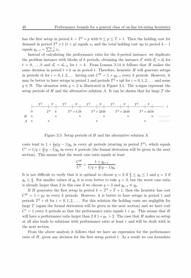
58

48 Performance bounds for a general class of on-line lot-sizing heuristics

has the first setup in period k = T 2 + p with 0 ≤ p ≤ T + 1. Then the holding cost for

demand in period T 2 + t (t < p) equals xt and the total holding cost up to period k − 1

equals yp−1 =∑p−1

t=0 xt.

Instead of calculating the performance ratio for the k-period instance, we duplicate

the problem instance with blocks of k periods, obtaining the instance d′ with d′t = dt for

t = 0, . . . , k and d′t = dt−k for t > k. From Lemma 3.14 it follows that H makes the

same decision in period t + k as in period t. Therefore, heuristic H will generate setups

in periods ik for i = 0, 1, 2, . . . having cost CH = 1 + yp−1 every k periods. However, it

may be better to have setups in period 1 and periods T 2 + iqk for i = 0, 1, 2, . . . and some

q ∈ N. The situation with q = 2 is illustrated in Figure 3.5. The x-signs represent the

setup periods of H and the alternative solution A. It can be shown that for large T the

T 2 T 2 T 2 T 2 T 2p p p p p

0 T 2 k T 2 + k T 2 + 2k T 2 + 3k T 2 + 4k2k 3k 4k 5k

t

H

A

x x x x x x

x x x x

.. .. . .. . .

. . . . . . . . .

Figure 3.5: Setup periods of H and the alternative solution A

costs tend to 1 + 12q(q − 1)yp in every qk periods (starting in period T 2), which equals

C∗ = 1/q + 12(q − 1)yp in every k periods (the formal derivation will be given in the next

section). This means that the worst case ratio equals at least

CH

C∗=

1 + yp−1

1/q + 12(q − 1)yp

.

It is not difficult to verify that it is optimal to choose q = 2 if 13≤ yp ≤ 1 and q = 3 if

yp ≤ 13. For smaller values of yp it is even better to take q > 3, but the worst case ratio

is already larger than 2 in this case if we choose q = 3 and yp−1 ≈ yp.

If H generates the first setup in period k = T 2 + T + 1, then the heuristic has cost

CH = 1 + yT in every k periods. However, it is better to have setups in period 1 and

periods T 2 + ik for i = 0, 1, 2, . . . . For this solution the holding costs are negligible for

large T (again the formal derivation will be given in the next section) and we have cost

C∗ = 1 every k periods so that the performance ratio equals 1 + yT . This means that H

will have a performance ratio larger than 2 if 1+yT > 2. The case that H makes no setup

at all also leads to solutions with performance ratio at least r and will be dealt with in

the next section.

From the above analysis it follows that we have an expression for the performance

ratio of H , given any decision for the first setup period t. As a result we can formulate

59

3.4 Analysis of heuristics satisfying Properties 1-3 49

the problem of finding a worst case example as an optimization problem. Let r be the

performance ratio. Then we want to solve the model

max r

s.t. r ≤ 1+yt−1

a(yt)t = 0, . . . , T

r ≤ 1 + yT

yt ≤ yt+1 t = 0, . . . , T − 1

y0 ≥ 0,

where

a(yt) =

12

+ 12yt if yt ≥ 1

313

+ yt if yt ≤ 13.

The first set of constraints deals with the case that H generates its first setup in some

period t + T 2 with 0 ≤ t ≤ T having performance ratio (1 + yt−1)/a(yt). The second

constraint handles the case with the first setup occurring in period T 2 + T + 1 having

performance ratio 1 + yt. The last two sets of constraints ensure that xt ≥ 0. Namely, if

we solve the model, then the variables xt (used to construct the problem instance d) can

be found by letting x0 = y0 and xt = yt − yt−1 for t > 0.

The model is a nonlinear optimization problem and hence difficult to solve in general.

However, we are able to use the model to find worst case examples. If we fix r, then

there exists a problem instance with performance ratio r if there exists a sequence yk that

satisfies the following constraints.

rat ≤ 1 + yt−1 t = 0, . . . , T

r ≤ 1 + yT

yt ≤ yt+1 t = 0, . . . , T − 1

y0 ≥ 0

at = 13z1

t + 23z2

t + 1z3t t = 0, . . . , T

yt = 0z1t + 1

3z2

t + 1z3t t = 0, . . . , T

z1t + z2

t + z3t = 1 t = 0, . . . , T

z1t ≤ 1 − bt t = 0, . . . , T

z3t ≤ bt t = 0, . . . , T

bt ∈ 0, 1 t = 0, . . . , T.

Note that the piecewise linear function a(yt) is modelled by the last six sets of constraints

and the variables at = a(yt), z1t , z2

t , z3t and the binary variables bt. If 0 ≤ yt ≤ 1

3, then yt

can be written as 0z1t + 1

3z2

t with z1t + z2

t = 1 and at = 13z1

t + 23z2. Similarly, if 1

3≤ yt ≤ 1,

then yt can be written as 13z2

t +1z3t with z2

t + z3t = 1 and at = 2

3z2

t +1z2. When yt ≤ 13

the

binary variable bt = 0 implying z3t = 0, and when yt ≥ 1

3we have bt = 1 implying z1

t = 0.

Thus for a fixed r, finding a problem instance reduces to finding a feasible solution

to a set of linear constraints consisting of binary and continuous variables. The largest

60

50 Performance bounds for a general class of on-line lot-sizing heuristics

value of r that satisfies these constraints can be found by performing a binary search.

Table 3.6 shows a feasible solution for r = 1.95 and T = 19. In the next section we will

t 0 1 2 3 4 5 6 7 8 9

xt 0.180 0.092 0.047 0.015 0.034 0.035 0.036 0.037 0.038 0.039

xt/xt−1 - 0.51 0.51 0.32 2.26 1.03 1.03 1.03 1.02 1.03

t 10 11 12 13 14 15 16 17 18 19

xt 0.040 0.041 0.042 0.043 0.044 0.045 0.046 0.048 0.049 0.050

xt/xt−1 1.03 1.03 1.03 1.03 1.03 1.02 1.02 1.03 1.03 1.02

Table 3.6: Feasible solution for T = 19 with r = 1.95

give a problem instance with r = 2 which is based on the values xt of Table 3.6.

3.4.2 The worst case problem instance

In this section we will prove that the worst case performance of each heuristic in our

special class is at least 2. In the proof we will use a demand sequence based on Table 3.6

and we will derive some properties for this sequence. Let n ∈ N be fixed and let xk = 16(1

2)k

for k = 0, . . . , n − 1 and xk = 23n

for k = n, . . . , 2n − 1. The terms xk are based on the

pattern observes in Table 3.6. For the first terms in this table it holds xt/xt−1 ≈ 12

and for

the last terms it holds xt/xt−1 ≈ 1. These are exactly the properties for xk as xk/xk−1 = 12

for k ≤ n − 1 and xk/xk−1 = 1 for k ≥ n + 1. Note that for t = 3 and t = 4 in Table 3.6

there is some deviation from this behavior. Finally, define the partial sum yk =∑k

i=0 xk.

Lemma 3.15 For 0 ≤ k ≤ n − 1 we have

1 + yk−1

13

+ yk

= 2. (3.12)

Proof First, note that (3.12) holds for k = 0 as 11/3+1/6

= 2. Assume that (3.12) holds

for some k ≥ 0 so that 23

+ 2yk = 1 + yk−1. Since 2xk+1 = xk we have

2

3+ 2yk + 2xk+1 = 1 + yk−1 + xk ⇔ 2

3+ 2yk+1 = 1 + yk ⇔ 1 + yk

13

+ yk+1

= 2.

Lemma 3.16 For n ≤ k ≤ 2n − 1 we have

1 + yk−1

12

+ 12yk

→ 2 for n → ∞.

61

3.4 Analysis of heuristics satisfying Properties 1-3 51

Proof Clearly,1 + yk−1

12

+ 12yk

=1 + yk

12

+ 12yk

− xk

12

+ 12yk

= 2 − xk

12

+ 12yk

and the lemma follows because xk = 23n

→ 0 for n → ∞.

Lemma 3.17 For n → ∞ we have y2n−1 → 1.

Proof

limn→∞

y2n−1 = limn→∞

n−1∑

k=0

1

6

(1

2

)k

+ limn→∞

2n−1∑

k=n

2

3n=

1

3+

2

3= 1.

Theorem 3.18 Every heuristic satisfying Properties 1-3 has worst case ratio at least 2.

Proof Consider a problem instance defined as follows: d0 > 0, dt = 0 (t = 2, . . . , T 2−1),

dt =x

t−T2

t(t = T 2, . . . , T 2 + T ), dT 2+T+1 = 1

T 2+T+1and dT 2+T+2 = 1

T 2+T+2and T = 2n.

Consider any heuristic H and let k > 0 be the first period where H makes a setup.

Dependent on the period k we will define an (possibly infinite) problem instance where

we not necessarily use the complete instance d. We will show that the performance ratio

of H for all problem instances tends to 2.

• k ∈ 1, . . . , T 2 − 1:Because it is optimal to have only a setup in period 0, the cost of the optimal

solution equals C∗ = 1. As the cost of H equals CH = 2, H has performance ratio

CH/C∗ = 2.

• k ∈ T 2, . . . , T 2 + n:Extend the k-period problem with dt = dt−k for t > k. Because of Lemma 3.14, H

will have setups in periods ik for i = 0, 1, 2, . . . with cost

CH = 1 +k−1∑

i=1

idi = 1 +k−1∑

i=T 2

xi = 1 + yk−1−T 2

62

52 Performance bounds for a general class of on-line lot-sizing heuristics

in every k periods. Now consider a solution with setups in period 1 and periods T 2+

i3k for i = 0, 1, 2, . . . . The holding cost of this solution for every 3k periods equals

3k+T 2−1∑

i=T 2

(i − T 2)di =

k∑

i=T 2

(i − T 2)di +

2k∑

i=T 2+k

(i − T 2)di +

3k∑

i=T 2+2k

(i − T 2)di

=

k∑

i=T 2

i − T 2

ixi−T 2 +

2k∑

i=T 2+k

i − T 2

i − kxi−T 2−k +

3k∑

i=T 2+2k

i − T 2

i − 2kxi−T 2−2k

≤k∑

i=T 2

T

T 2xi−T 2 +

2k∑

i=T 2+k

T 2 + 2T

T 2xi−T 2−k +

3k∑

i=T 2+2k

2T 2 + 3T

T 2xi−T 2−2k

=

(3 +

6

T

) k−T 2∑

i=0

xi =

(3 +

6

T

)yk−T 2,

where the inequality follows from k − T 2 ≤ T . So the average cost for every k

periods equals

C∗ ≤ 1

3+

(1 +

2

T

)yk−T 2.

As k − 1 − T 2 ≤ n − 1, by Lemma 3.15 we have that

CH

C∗≥ 1 + yk−1−T 2

13

+ yk−T 2 + 2Tyk−T 2

→ 2 for T → ∞.

• k ∈ T 2 + n + 1, . . . , T 2 + T:Extend the k-period problem with dt = dt−k for t > k. As in the previous case H will

have setups in periods ik for i = 0, 1, 2, . . . with cost CH = 1 + yk−1−T 2 in every k

periods. Now consider a solution with setups in period 1 and periods T 2 + i2k for

i = 0, 1, 2, . . . . By a similar argument as in the previous case the holding cost of

this solution for every 2k periods equals at most(1 + 3

T

)yk−T 2. So the average cost

for every k periods equals

C∗ ≤ 1

2+

(1

2+

3

2T

)yk−T 2.

As n ≤ k − 1 − T 2 ≤ 2n − 1, by Lemma 3.16 we have that

CH

C∗≥ 1 + yk−1−T 2

12

+ 12yk−T 2 + 3

2Tyk−T 2

→ 2 for T → ∞.

• k = T 2 + T + 1:

Again we extend the k-period problem with dt = dt−k for t > k. Heuristic H

63

3.4 Analysis of heuristics satisfying Properties 1-3 53

will generate setups in periods ik for i = 0, 1, 2, . . . with cost CH = 1 + yT in

every k periods. Consider a solution with setups in period 1 and periods T 2 + ik

for i = 0, 1, 2, . . . . This solution has cost C∗ = 1 +∑T 2+T

i=T 2 (i − T 2)di + T+1T 2+T+1

≤1 + 1

TyT + 1

T≤ 1 + 2

Tas yT ≤ 1. By Lemma 3.17 we have

CH

C∗≥ 1 + yT

1 + 2T

→ 2 for T → ∞.

• k = T 2 + T + 2 or there is no setup:

In both cases the total costs of the heuristic equal CH = 3+yT for the (T 2 +T +2)-

period problem. By Lemma 3.17 we have CH → 4 for T → ∞. Consider a solution

with setups in periods 1 and T 2. Then the cost of this solution C∗ ≤ 2 + 1TyT +

T+1T 2+T+1

+ T+2T 2+T+2

→ 2 as T → ∞ concluding that

CH

C∗→ 2 for T → ∞.

In conclusion, no matter where the first setup (after period 0) occurs, we can always con-

struct a problem instance with performance ratio 2 and hence the worst case performance

of any heuristic in our class is at least 2.

3.4.3 Implications

Look-ahead look-back heuristics

The heuristics in our class are myopic in the sense that they do not take into account

future demand. However, there is a broader class of heuristics which has a so-called look

ahead-look back feature. When the decision is to make a setup in period t or not, there

is an option to look back and look ahead a number of periods and to move the setup

to one of those periods if an improvement can be made. Wemmerlov (1983) proposes a

variant of the PPB where it is allowed to look ahead and look back one period in order to

improve the current solution. Heuristics possessing the look ahead-look back feature can

be considered as a compromise between the class of myopic heuristics and the heuristics

using the complete model horizon.

Consider a heuristic satisfying Properties 1-3 with the additional option to look ahead

and look back l perriods. A slightly modified version of the worst case example of Sec-

tion 3.4.2 shows that heuristics with the look ahead-look back feature also have worst case

ratio at least two. Let d = d0, . . . , dT 2+T+2 be the demand sequence used in the proof of

Theorem 3.18. Now define the sequence d′ with d′(l+1)t = dt/(l+1) for t = 0, . . . , T 2+T +2

and let the remaining demands be equal to zero. So we have added l zero-demand periods

between every two positive demand periods.

64

54 Performance bounds for a general class of on-line lot-sizing heuristics

Assume that some heuristic generates the first setup in some period q = p(l + 1)

with p ∈ N. When looking back or looking ahead l periods, there are only zero-demand

periods and hence cost will not decrease when moving the setup to one of these periods.

Furthermore, the holding cost for some period r(l + 1) with r < p equals r(l + 1)d′r(l+1) =

r(l + 1)dr/(l + 1) = rdr, which is the holding cost for demand dr in problem instance d

when it is produced in period 0. So the holding costs up to period q for instance d′ with

the first setup in period 0 are equal to the holding costs up to period p for instance d

with the first setup in period 0. Therefore, starting with instance d′ and applying similar

arguments as in the proof of Theorem 3.18 shows that our class of heuristics with an

additional look ahead-look back feature also has worst case ratio at least two. Thus the

following corollary follows from the above discussion.

Corollary 3.19 Let H be a heuristic satisfying Properties 1-3 with the additional property

to look ahead and look back l periods for some fixed l > 0. Then H has worst case ratio

at least 2.

Rolling horizon environment

Often the demand for the complete horizon T is not known, but the demand for the

first n periods is known. In this case the lot-sizing problem for n periods is solved, the

first lot-size decision is implemented and the horizon is rolled forward to the period where

the next lot-size starts. Again it is assumed that the next n periods are known and

the procedure is repeated. This is known as lot-sizing in a rolling horizon environment,

where n is called the planning horizon. As the heuristics within our class use no future

demand information, they are suitable to be applied in a rolling horizon environment.

Consider a rolling horizon environment with a planning horizon of n periods. We can

easily construct a problem instance with worst case performance arbitrary large. Take

the instance with dtn = ε for t = 0, 1, 2, . . . and zero demands elsewhere. In period 0

any algorithm faces zero demands in all periods except for period 0 and hence a lot-size

of ε is made in period 0. Now the horizon is rolled forward to period n and we are in

the same situation as in period 0. So any heuristic will generate a solution with setups

in periods tn for t = 0, 1, 2, . . . . Clearly, the worst case performance becomes arbitrary

large, as it is optimal to have only a setup in period 0 for ε sufficiently small.

The deficiency of any algorithm is that no solution with a lot-size covering more than n

periods can be constructed, whereas it may be optimal to have lot-sizes that cover more

than n periods. In the latter case the optimal solution can never be constructed by any

algorithm in a rolling horizon environment with planning horizon n. This is in contrast

with the situation where the planning horizon is not bounded. In this case the heuristics

make the setups in the wrong periods, while it is possible to construct a solution with the

same setups as in the optimal solution.

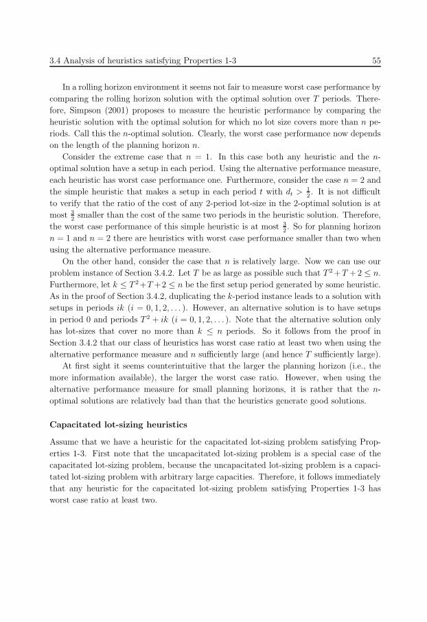
65

3.4 Analysis of heuristics satisfying Properties 1-3 55

In a rolling horizon environment it seems not fair to measure worst case performance by

comparing the rolling horizon solution with the optimal solution over T periods. There-

fore, Simpson (2001) proposes to measure the heuristic performance by comparing the

heuristic solution with the optimal solution for which no lot size covers more than n pe-

riods. Call this the n-optimal solution. Clearly, the worst case performance now depends

on the length of the planning horizon n.

Consider the extreme case that n = 1. In this case both any heuristic and the n-

optimal solution have a setup in each period. Using the alternative performance measure,

each heuristic has worst case performance one. Furthermore, consider the case n = 2 and

the simple heuristic that makes a setup in each period t with dt > 12. It is not difficult

to verify that the ratio of the cost of any 2-period lot-size in the 2-optimal solution is at

most 32

smaller than the cost of the same two periods in the heuristic solution. Therefore,

the worst case performance of this simple heuristic is at most 32. So for planning horizon

n = 1 and n = 2 there are heuristics with worst case performance smaller than two when

using the alternative performance measure.

On the other hand, consider the case that n is relatively large. Now we can use our

problem instance of Section 3.4.2. Let T be as large as possible such that T 2 +T +2 ≤ n.

Furthermore, let k ≤ T 2+T +2 ≤ n be the first setup period generated by some heuristic.

As in the proof of Section 3.4.2, duplicating the k-period instance leads to a solution with

setups in periods ik (i = 0, 1, 2, . . . ). However, an alternative solution is to have setups

in period 0 and periods T 2 + ik (i = 0, 1, 2, . . . ). Note that the alternative solution only

has lot-sizes that cover no more than k ≤ n periods. So it follows from the proof in

Section 3.4.2 that our class of heuristics has worst case ratio at least two when using the

alternative performance measure and n sufficiently large (and hence T sufficiently large).

At first sight it seems counterintuitive that the larger the planning horizon (i.e., the

more information available), the larger the worst case ratio. However, when using the

alternative performance measure for small planning horizons, it is rather that the n-

optimal solutions are relatively bad than that the heuristics generate good solutions.

Capacitated lot-sizing heuristics

Assume that we have a heuristic for the capacitated lot-sizing problem satisfying Prop-

erties 1-3. First note that the uncapacitated lot-sizing problem is a special case of the

capacitated lot-sizing problem, because the uncapacitated lot-sizing problem is a capaci-

tated lot-sizing problem with arbitrary large capacities. Therefore, it follows immediately

that any heuristic for the capacitated lot-sizing problem satisfying Properties 1-3 has

worst case ratio at least two.

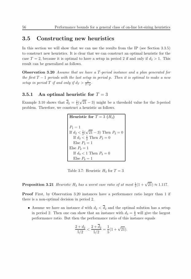
66

56 Performance bounds for a general class of on-line lot-sizing heuristics

3.5 Constructing new heuristics

In this section we will show that we can use the results from the IP (see Section 3.3.5)

to construct new heuristics. It is clear that we can construct an optimal heuristic for the

case T = 2, because it is optimal to have a setup in period 2 if and only if d2 > 1. This

result can be generalized as follows.

Observation 3.20 Assume that we have a T -period instance and a plan generated for

the first T − 1 periods with the last setup in period p. Then it is optimal to make a new

setup in period T if and only if dT > 1T−p

.

3.5.1 An optimal heuristic for T = 3

Example 3.10 shows that d2 = 15(√

21 − 3) might be a threshold value for the 3-period

problem. Therefore, we construct a heuristic as follows.

Heuristic for T = 3 (H3)

P1 = 1

If d2 < 12(√

21 − 3) Then P2 = 0

If d3 < 12

Then P3 = 0

Else P3 = 1

Else P2 = 1

If d3 < 1 Then P3 = 0

Else P3 = 1

Table 3.7: Heuristic H3 for T = 3

Proposition 3.21 Heuristic H3 has a worst case ratio of at most 15(1 +

√21) ≈ 1.117.

Proof First, by Observation 3.20 instances have a performance ratio larger than 1 if

there is a non-optimal decision in period 2.

• Assume we have an instance d with d2 < d2 and the optimal solution has a setup

in period 2. Then one can show that an instance with d3 = 12

will give the largest

performance ratio. But then the performance ratio of this instance equals

2 + d2

5/2<

2 + d2

5/2=

1

5(1 +

√21).

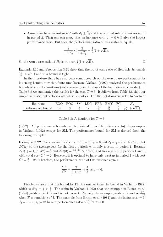
67

3.5 Constructing new heuristics 57

• Assume we have an instance d with d2 ≥ d2 and the optimal solution has no setup

in period 2. Then one can show that an instance with d3 = 0 will give the largest

performance ratio. But then the performance ratio of this instance equals

2

1 + d2≤ 2

1 + d2

=1

5(1 +

√21).

So the worst case ratio of H3 is at most 15(1 +

√21).

Example 3.10 and Proposition 3.21 show that the worst case ratio of Heuristic H3 equals15(1 +

√21) and this bound is tight.

In the literature there has also been some research on the worst case performance for

lot-sizing heuristics with a finite time horizon. Vachani (1992) analyzed the performance

bounds of several algorithms (not necessarily in the class of the heuristics we consider). In

Table 3.8 we summarize the results for the case T = 3. It follows from Table 3.8 that our

simple heuristic outperforms all other heuristics. For the notations we refer to Vachani

Heuristic EOQ POQ SM LUC PPB BMY FC H3

Performance bound ∞ 3 43

∞ 32

32

65

15(1 +

√21)

Table 3.8: A heuristic for T = 3

(1992). All performance bounds can be derived from (the references to) the examples

in Vachani (1992) except for SM. The performance bound for SM is derived from the

following example.

Example 3.22 Consider an instance with d1 = 1, d2 = 0 and d3 = 14+ ε with ε > 0. Let

AC(t) be the average cost for the first t periods with only a setup in period 1. Because

AC(1) = 1, AC(2) = 12

and AC(3) = 3/2+2ε3

> AC(2), SM has a setup in periods 1 and 3

with total cost CH = 2. However, it is optimal to have only a setup in period 1 with cost

C∗ = 32

+ 2ε. Therefore, the performance ratio of this instance equals

CH

C∗=

232

+ 2ε→ 4

3as ε → 0.

Finally, we note that the bound for PPB is smaller than the bound in Vachani (1992)

which is 3TT+2

= 95

> 32. The claim in Vachani (1992) that the example in Bitran et al.

(1984) yields a tight bound is not correct. Namely the example yields a bound of 3TT+3

when T is a multiple of 3. The example from Bitran et al. (1984) and the instance d1 = 1,

d2 = 1 − ε, d3 = 2ε have a performance ratio of 32

for ε → 0.

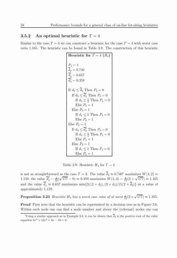
68

58 Performance bounds for a general class of on-line lot-sizing heuristics

3.5.2 An optimal heuristic for T = 4

Similar to the case T = 3 we can construct a heuristic for the case T = 4 with worst case

ratio 1.165. The heuristic can be found in Table 3.9. The construction of this heuristic

Heuristic for T = 4 (H4)

P1 = 1

d2 = 0.740

d1

3 = 0.657

d2

3 = 0.359

If d2 ≤ d2 Then P2 = 0

If d3 ≤ d1

3 Then P3 = 0

If d4 ≤ 13

Then P4 = 0

Else P4 = 1

Else P3 = 1

If d4 ≤ 1 Then P4 = 0

Else P4 = 1

Else P2 = 1

If d3 ≤ d2

3 Then P3 = 0

If d4 ≤ 12

Then P4 = 0

Else P4 = 1

Else P3 = 1

If d4 ≤ 1 Then P4 = 0

Else P4 = 1

Table 3.9: Heuristic H4 for T = 4

is not as straightforward as the case T = 3. The value d2 ≈ 0.7401 maximizes W (4, 2) ≈1.150, the value d

2

3 = 122

(√

177 − 9) ≈ 0.359 maximizes W (4, 3) = 114

(3 +√

177) ≈ 1.165

and the value d1

3 ≈ 0.657 maximizes min3/(2 + d3), (3 + d3)/(5/2 + d2) at a value of

approximately 1.129.

Proposition 3.23 Heuristic H4 has a worst case ratio of at most 114

(3+√

177) ≈ 1.165.

Proof First note that the heuristic can be represented by a decision tree as in Figure 3.6.

Within each node one can find a node number and above the (relevant) nodes one can

1Using a similar approach as in Example 3.8, it can be shown that d2 is the positive root of the cubic

equation 3x3 + 12x2 + 3x − 10 = 0.

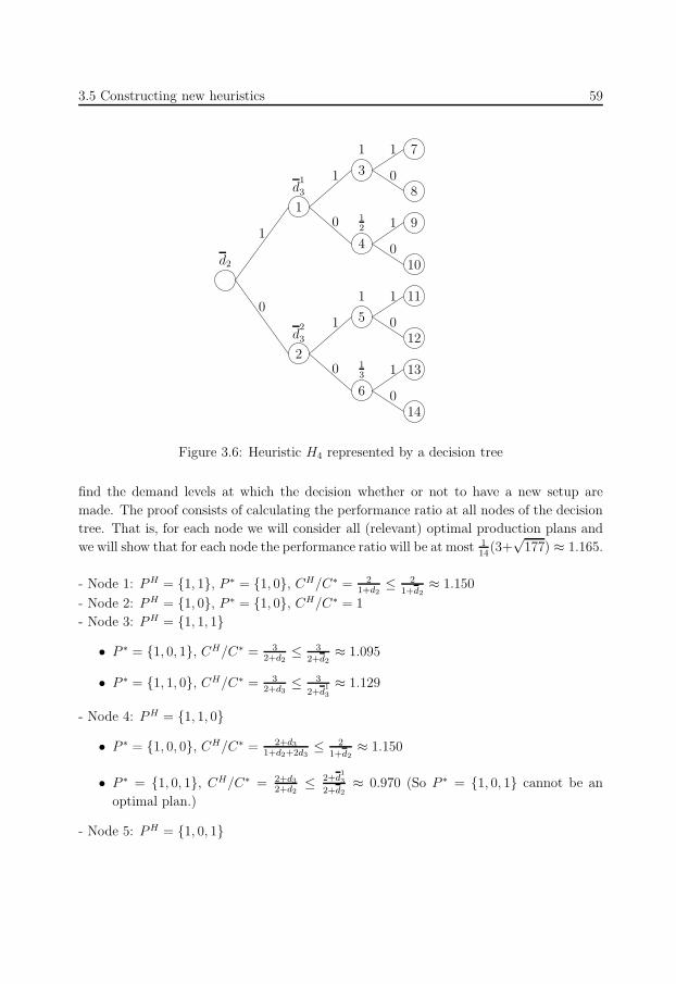
69

3.5 Constructing new heuristics 59

7

8

9

10

11

12

13

14

3

4

5

6

1

2

d2

d1

3

d2

3

1

1

12

13

1

1

1

1

1

1

10

0

0

0

0

0

0

Figure 3.6: Heuristic H4 represented by a decision tree

find the demand levels at which the decision whether or not to have a new setup are

made. The proof consists of calculating the performance ratio at all nodes of the decision

tree. That is, for each node we will consider all (relevant) optimal production plans and

we will show that for each node the performance ratio will be at most 114

(3+√

177) ≈ 1.165.

- Node 1: P H = 1, 1, P ∗ = 1, 0, CH/C∗ = 21+d2

≤ 21+d2

≈ 1.150

- Node 2: P H = 1, 0, P ∗ = 1, 0, CH/C∗ = 1

- Node 3: P H = 1, 1, 1

• P ∗ = 1, 0, 1, CH/C∗ = 32+d2

≤ 32+d2

≈ 1.095

• P ∗ = 1, 1, 0, CH/C∗ = 32+d3

≤ 3

2+d1

3

≈ 1.129

- Node 4: P H = 1, 1, 0

• P ∗ = 1, 0, 0, CH/C∗ = 2+d3

1+d2+2d3≤ 2

1+d2

≈ 1.150

• P ∗ = 1, 0, 1, CH/C∗ = 2+d3

2+d2≤ 2+d

1

3

2+d2

≈ 0.970 (So P ∗ = 1, 0, 1 cannot be an

optimal plan.)

- Node 5: P H = 1, 0, 1

70

60 Performance bounds for a general class of on-line lot-sizing heuristics

• P ∗ = 1, 0, 0, CH/C∗ = 2+d2

1+d2+2d3≤ 2

1+2d2

3

≈ 1.165

• P ∗ = 1, 1, 0, CH/C∗ = 2+d2

2+d3≤ 2+d2

2+d2

3

≈ 1.162

- Node 6: P H = 1, 0, 0

• P ∗ = 1, 0, 1, CH/C∗ = 1+d2+2d3

2+d2≤ 1+2d

2

3

2≈ 0.859 (So P ∗ = 1, 0, 1 cannot be an

optimal plan.)

• P ∗ = 1, 1, 0, CH/C∗ = 1+d2+2d3

2+d3≤ 1+d2+2d

2

3

2+d2

3

≈ 1.042

For nodes 7–14 we note that the case with P ∗4 = 1 is not of interest. Because the cost

in period 4 of the optimal solution is always at least equal to the cost in period 4 of the

heuristic solution, the performance ratios will be at most equal to the performance ra-

tios of the 3-period problems (that is, the performance ratios corresponding to nodes 3–6).

- Nodes 7 and 11: Because both the heuristic and the optimal solution have a setup in

period 4 (as d4 > 1), the performance ratios will be smaller than the performance ratios

of nodes 3 and 5, respectively.

- Node 8: P H = 1, 1, 1, 0, P ∗ = 1, 0, 1, 0, CH/C∗ = 3+d4

2+d2+d4≤ 3

2+d2

≈ 1.095

- Node 9: P H = 1, 1, 0, 1, P ∗ = 1, 0, 1, 0, CH/C∗ = 3+d3

2+d2+d4≤ 3+d

1

3

2+d2+ 1

2

≈ 1.129

- Node 10: P H = 1, 1, 0, 0

• P ∗ = 1, 0, 0, 0, CH/C∗ = 2+d3+2d4

1+d2+2d3+3d4≤ 2

1+d2

≈ 1.150

• P ∗ = 1, 0, 1, 0, CH/C∗ = 2+d3+2d4

2+d2+d4≤ 2+d

1

3+2· 12

2+d2+1

2

≈ 1.129

- Node 12: P H = 1, 0, 1, 0

• P ∗ = 1, 0, 0, 0, CH/C∗ = 2+d2+d4

1+d2+2d3+3d4≤ 2

1+2d2

3

≈ 1.165

• P ∗ = 1, 1, 0, 0, CH/C∗ = 2+d2+d4

2+d3+2d4≤ 2+d2

2+d2

3

≈ 1.162

- Node 13: P H = 1, 0, 0, 1

• P ∗ = 1, 1, 0, 0, CH/C∗ = 2+d2+2d3

2+d3+2d4≤ 2+d2+2d

2

3

2+d2

3+2· 13

≈ 1.143

• P ∗ = 1, 0, 1, 0, CH/C∗ = 2+d2+2d3

2+d2+d4≤ 2+2d

2

3

2+ 1

3

≈ 1.165

- Node 14: P H = 1, 0, 0, 0

71

3.6 Conclusion & Future research 61

• P ∗ = 1, 1, 0, 0, CH/C∗ = 1+d2+2d3+3d4

2+d3+2d4≤ 1+d2+2d

2

3+3· 13

2+d2

3+2· 13

≈ 1.143

• P ∗ = 1, 0, 1, 0, CH/C∗ = 1+d2+2d3+3d4

2+d2+d4≤ 1+2d

2

3+3· 13

2+ 1

3

≈ 1.165

Note that if d2 > d2, then we already know in the second period that the performance

ratio will be smaller or equal than 1.150. This is because there is a relatively high cost in

period 2 (at least d2), which causes a relatively small performance ratio.

3.6 Conclusion & Future research

In this chapter we studied the worst case performance for a general class of on-line lot-

sizing heuristics. We showed that heuristics whick make lot-sizing decisions on a period-

by-period basis have a worst case ratio of at least 32, even if the optimal solution and the

heuristic solution have at most 2 setups (including the setup in the first period). Using the

analysis to construct the worst case examples enabled us to find heuristics with optimal

worst case performance for three- and four-period problem instances.

Furthermore, deterministic heuristics that make decisions only based on the current

lot-size on a period-by-period basis have worst case ratio at least 2. This result generalizes

the result of Axsater (1985), who shows that a more restrictive class of heuristics has worst

case ratio at least 2. The problem instance with this performance behavior was found by

formulating the problem of finding worst case examples as a MIP.

We conclude this chapter with some issues for further research. First, the question

is still open whether there exist on-line heuristics with a worst case performance strictly

smaller than 2. We showed that the worst case performance of such heuristics is at least 32,

but no heuristics are known in the literature with worst case performance smaller than 2.

Clearly, there is a gap to be closed here. Second, for the 3- and 4-period problem we

constructed heuristics with optimal worst case performance. The question is: can we

generalize this to arbitrary model horizons? In the proofs for the 3- and 4-period case we

considered all possible production plans, which grow at an exponential rate. Therefore,

to answer the last question one will need another proof strategy.

72

73

Part II

Economic lot-sizing and pricing

74

75

Introduction 65

Introduction

The demand that a manufacturer has to satisfy is usually created by activities of its

marketing department. Instead of taking the marketing and production decisions more

or less independently, it may be beneficial to integrate these decisions. This leads to

models that are more complex than when we are only concerned with optimal production

decisions. As an example, suppose that the selling price of the item still has to be set

and that the demand functions are given for the periods under consideration. Then the

planning problem consists of deciding simultaneously how high to set the price and how

much to produce in each period such that the total profit is maximized.

In this part of the thesis we consider the economic lot-sizing (ELS) problem where

demand can be affected by pricing. So instead of assuming that demand is deterministic

as in the classical ELS problem, we assume that demand is a deterministic function of

the price (assuming some market power of the manufacturer). We will call this the joint

pricing and lot-sizing problem.

We see in the literature that two pricing assumptions are made. First, one can assume

that a different price can be set in each period. For instance, this is the case for a

monopolist. Thomas (1970) showed that this problem can be solved in a similar way as

the well-known algorithm proposed by Wagner and Whitin (1958). For instance, if demand

is assumed to be linear in the price, then the algorithm requires O(T 2) computation time.

This means that this problem can still be solved efficiently.

Another assumption is that a single price must be set for all periods. For instance, this

is the case if firms rely on sales from catalogues. In this case it may be rather expensive

to communicate price changes to the customers. Kunreuther and Schrage (1973) propose

a heuristic algorithm to solve this problem. However, they do not give any approximation

and complexity results of their algorithm. Gilbert (1999) proposes an exact algorithm

to solve this problem in O(T 3) time, but imposes some additional restrictions on the

demand and cost parameters. In a more recent paper Gilbert (2000) considers the case

with multiple items and production capacities. In that paper it is assumed that setup

costs are negligible. The problem is solved iteratively by using the dual problem of the

production scheduling problem.

Recently, two papers appeared on a joint pricing and lot-sizing model with the general-

ization to account for time-invariant production capacities. Geunes et al. (2006) consider

a model where the revenue functions are assumed to be piecewise linear concave in the

demand level. They show that the problem can be solved in polynomial time. In Geunes

et al. (2005) it is shown that this result still holds for arbitrary concave revenue functions,

which generalizes the result of Thomas (1970). Furthermore, Geunes et al. (2005) also

generalize the work of Kunreuther and Schrage (1973), Gilbert (1999) and Van den Heuvel

76

66 Introduction

and Wagelmans (2006b) by showing that their models with the inclusion of time-invariant

capacities can still be solved in polynomial time.

Besides the assumption on pricing, we can distinguish other differences between mar-

keting-production models. For example, demand may depend on other marketing instru-

ments than price such as promotion. Sogomonian and Tang (1993) consider a T -period

discrete model where the promotion periods and promotion levels have to be determined.

A solution of the model is found by solving a number of nested longest path problems.

Another distinction in models is that between discrete time and continuous time models.

Whitin (1955) considers a pricing problem in the EOQ framework. Finally, there is also

literature on marketing-production models in a stochastic environment. For an overview

of literature on marketing-production decision-making models we refer to Eliashberg and

Steinberg (1993).

In Chapters 4 and 5 we will consider a joint pricing and lot-sizing model. In Chapter 4

we consider the problem where prices may vary over time. In particular, we will focus

on a problem with a time-invariant demand function and time-invariant cost parameters.

Although Bhattacharjee and Ramesh (2000) proposed a heuristic approach, we will show

that the problem can be solved to optimality in a practically efficient way. In Chapter 5

we consider the joint pricing and lot-sizing problem where the price has to be constant

over time. By refining the algorithm of Kunreuther and Schrage (1973) we will show that

the problem can be solved in polynomial time.

77

Chapter 4

A joint pricing and lot-sizing model

with general prices over time∗

Abstract

In this chapter we consider a joint pricing and lot-sizing model. It is assumed

that demand is a (deterministic) function of price, where prices may vary over

time. We focus on a special case with time-invariant cost parameters considered

by Bhattacharjee and Ramesh (2000). While Bhattacharjee and Ramesh (2000)

proposed two heuristics, we show that the problem can be solved by a (practically)

efficient algorithm proposed by Thomas (1970). Moreover, the problem can be

solved even faster by applying the results on a special partition problem derived by

Orlin (1985).

4.1 Introduction

In this chapter we consider a joint pricing and lot-sizing model for a manufacturer who

is dealing in a single product. It is assumed that the manufacturer has some monopo-

listic power and he can affect his demand by pricing. For a given planning horizon the

manufacturer wants to maximize his profit considering revenue and all relevant costs.

The problem is to simultaneously make pricing and lot-sizing decisions such that profit is

maximized.

In this chapter we focus on a special case of the problem considered by Bhattacharjee

and Ramesh (2000) with time-invariant cost and demand parameters. Bhattacharjee and

Ramesh (2000) proposed two heuristic algorithms to solve this special case of the problem.

In this chapter we improve on their paper by showing that the problem can be solved to

optimality in a (practically) efficient way. We do this by applying (a slightly modified

∗This chapter is based on Van den Heuvel and Wagelmans (2003).

78

68 A joint pricing and lot-sizing model with general prices over time

version of) the approach of Thomas (1970). Moreover, we show that an even faster method

exists when we apply the results on a special partition problem derived by Orlin (1985).

This chapter is organized as follows. In Section 4.2 we describe the joint pricing and

lot-sizing model considered by Bhattacharjee and Ramesh (2000) and give a mathematical

formulation. In Section 4.3 we present the exact method proposed by Thomas (1970) and

in Section 4.4 we apply this method to the Bhattacharjee and Ramesh (2000) case. In

Section 4.5 we introduce a special case of a partition problem and in Section 4.6 we

show how to apply the results for this problem to solve the Bhattacharjee and Ramesh

(2000) case even faster. In Section 4.7 we point out some concerns about the main results

presented by Bhattacharjee and Ramesh (2000). The chapter is ended with the conclusion

in Section 4.8.

4.2 Problem description

We consider the following joint pricing and lot-sizing model of Bhattacharjee and Ramesh

(2000). There is a monopolistic manufacturer dealing in a single product over a finite

time horizon. At the beginning of each period lot-sizing and pricing decisions are made,

where in each period a different price can be set. It is assumed that demand satisfies

d(p) = βp−α, (4.1)

where α > 1 is the demand elasticity, β > 0 is a constant and p is the price, where price in

each period t may be bounded from above or below, i.e., pmin ≤ pt ≤ pmax. The objective

of the manufacturer is to maximize his profit, i.e., to find the best price for which revenue

minus cost is maximized. Costs include a fixed setup cost for each period with positive

production and a unit production cost for each item produced. Furthermore, holding cost

is incurred for carrying inventory from a period to the next period. Bhattacharjee and

Ramesh (2000) assume that the cost parameters are time-invariant.

Assuming that all demand must be satisfied (i.e., loss of demand is not allowed) and

using the following notation,

T = model horizon

K = fixed setup cost

c = per unit production cost

h = holding cost per unit per period

pt = price set in period t

d(pt) = demand in period t when price equals pt

qt = produced quantity in period t

It = ending inventory in period t,

79

4.3 Solution approach by Thomas (1970) 69

the problem can be formulated as follows

max∑T

t=1 d(pt)pt − C(D(p))

s.t. pmin ≤ pt ≤ pmax t = 1, . . . , T,(4.2)

whereC(D(p)) = min

∑Tt=1 (Kδ(qt) + cqt + hIt)

s.t. It = It−1 − d(pt) + qt t = 1, . . . , T

qt, It ≥ 0 t = 1, . . . , T

I0 = 0,

with

δ(x) =

0 for x = 0

1 for x > 0

and D(p) is the demand vector D(p) = [d(p1), . . . , d(pT )].

In problem (4.2) we maximize the total revenue minus total cost over all periods, where

there may be bounds on the price. If price is not restricted, then we set pmin = 0 and

pmax = ∞ in the model. The total cost is represented by C(D(p)), which is the cost of a

‘standard’ economic lot-sizing (ELS) problem (Wagner and Whitin, 1958). We minimize

setup, unit production and holding costs, such that demand is satisfied and production

quantity and ending inventory are non-negative in each period. Furthermore, we may

assume without loss of generality that starting inventory is zero.

4.3 Solution approach by Thomas (1970)

In this section we give a brief description of the exact algorithm by Thomas (1970) to

solve the joint pricing and lot-sizing problem. Note that Thomas (1970) presented the

model as a minimization problem, whereas we present it as a maximization model (in

line with the formulation of (4.2)). Furthermore, Thomas (1970) assumed general cost

parameters and no bounds on the prices in each period.

Let a subplan be a consecutive number of periods for which demand is satisfied.

Thomas (1970) shows that the optimal solution consists of a series of consecutive subplans

as in the ELS problem. For a subplan consisting of periods j, . . . , t (1 ≤ j ≤ t ≤ T ) define

pjt as the price vector pjt = [pj, . . . , pt] and define πjt(pjt) as the total profit if production

takes place in period j to satisfy demand in periods j, . . . , t, i.e.,

πjt(pjt) =

t∑

k=j

[pk − cj −k−1∑

i=j

hi]dk(pk) − Kj. (4.3)

Furthermore, define πjt as the maximum profit for a subplan consisting of periods j, . . . , t,

i.e.,

πjt = maxpjt

πjt(pjt). (4.4)

80

70 A joint pricing and lot-sizing model with general prices over time

Thomas (1970) shows that if a setup takes place in period j and the next setup in

period t + 1, then the optimal price for period k = j, . . . , t must be set at the value p∗kthat maximizes

πk(pk) = (pk − cj −k−1∑

i=j

hi)dk(pk)

and hence

πjt =t∑

k=j

πk(p∗k) − Kj . (4.5)

Dependent on the structure of dt(pt) we can calculate this optimal price in an analytical

way or, if necessary, by enumeration. Throughout this chapter, we assume that this

problem is tractable.

Let F (t) be the optimal profit up to period t. As there exists an optimal solution

consisting of a series of consecutive subplans, the following forward recursion enables us

to find the optimal profit for the whole model horizon:

F (t) = maxj=1,...,t

F (j − 1) + πjt for t = 1, . . . , T with F (0) = 0. (4.6)

It is not difficult to see that, given the values πjt, this algorithm runs in O(T 2) time.

4.4 Applying Thomas’ approach to the Bhattachar-

jee and Ramesh (2000) case

In this section we apply Thomas’ approach to the Bhattacharjee and Ramesh (2000)

case. With their assumptions we can find the optimum of (4.3) in an analytical way.

Substituting demand function (4.1) and the time-invariant cost parameters (i.e., Kt = K,

ct = c and ht = h for t = 1, . . . , T ) in (4.3) we have that

πjt(pjt) =t∑

k=j

[pk − c −k−1∑

i=j

h]βp−αk − K =

t∑

k=j

[pk − c − (k − j)h]βp−αk − K. (4.7)

Calculating the first order conditions for the subplan consisting of periods i = j, . . . , t we

have

∂πjt(pjt)

∂pi= 0 ⇒ p∗i =

α(c + (i − j)h)

α − 1≥ 0 as α > 1, i ≥ j and c, h ≥ 0. (4.8)

Note that p∗i is not dependent on the prices set in the other periods of the subplan.

Furthermore, note that p∗i does only depend on period j and not on period t, which

implies that the optimal price for a single period is only dependent on the starting period

81

4.4 Applying Thomas’ approach to the Bhattacharjee and Ramesh (2000) case 71

of the subplan and independent of the number of periods in the subplan. Finally, one can

verify that

∂πjt(pjt)

∂pi

∣∣∣∣pi

> 0 for pi < p∗i and∂πjt(pjt)

∂pi

∣∣∣∣pi

< 0 for pi > p∗i .

This implies that the maximum profit function for a single period in a subplan is unimodal

and that it has a unique optimum at price p∗i .

If we analyze the second order partial derivative we find

∂2πjt(pjt)

∂pi2

= 0 ⇒ pi =(α + 1)(c + (i − j)h)

α − 1> p∗i .

It is not difficult to verify that the second order partial derivative is smaller than zero for

pi < pi and larger than zero for pi > pi. This means that the maximum profit function

for a single period in a subplan is concave for pi < pi and convex for pi > pi.

Because Bhattacharjee and Ramesh (2000) assume a time-invariant demand function

and time-invariant cost parameters, it follows from (4.3) and (4.8) that

πjt = π1,t−j+1 for all 1 ≤ j ≤ t ≤ T. (4.9)

This means that it is only necessary to evaluate π1t for t = 1, . . . , T . The following

recursion formulas can be used to calculate π1t for t = 1, . . . , T in O(T ) time:

p∗t+1 = p∗t +αh

α − 1(4.10)

π1,t+1 = π1,t + (p∗t+1 − c − th)β(p∗t+1

)−α(4.11)

with

p∗1 =αc

α − 1and π11 = (p∗1 − c)β (p∗1)

−α − K.

By applying recursion formula (4.6) and using (4.10) and (4.11), we can find the optimal

total profit, the optimal subplans and the optimal prices.

It follows from (4.10) that prices in consecutive periods within a subplan have an

interesting property: the difference between consecutive prices is constant as p∗i+1 − p∗i =αh

α−1. This means that even in the case of time-invariant demand functions and time-

invariant demand parameters, prices are not constant over time (as also noted in Geunes

et al. (2005)). The above property does not only hold for production cost functions with

a setup and unit production cost, but for arbitrary production cost functions.

Theorem 4.1 Consider a subplan 1, . . . , t with aggregate demand D. Then, given any

production cost function f , the prices that maximize the profit of the subplan satisfy p∗i+1−p∗i = αh

α−1.

82

72 A joint pricing and lot-sizing model with general prices over time

Proof Let f be an arbitrary production cost function and consider the problem

maxt∑

k=1

[pk − (k − 1)h]βpk−α − f(D)

s.t.t∑

k=1

βpk−α = D,

which maximizes the total profit of the subplan. Introducing the Lagrangian multiplier λ,

the following set of equations solves the optimization problem:

∂∂pi

[∑t

k=1(pk − (k − 1)h)βpk−α − f(D)] + λ ∂

∂pi[D −∑t

k=1 βpk−α] = 0 for i = 1, . . . , t,

∑tk=1 βpk

−α = D.

After some algebra the first set of equations reduces to

p∗i =αh(i − 1)

α − 1+ λ

α

α − 1for i = 1, . . . , t

and it follows that p∗i+1 − p∗i = αhα−1

.

Given some aggregate demand level D, there is a straightforward way to find the

optimal prices. Because all prices can be expressed in p1, i.e., pk = α(k−1)hα−1

+ p1, solving∑tk=1 βpk

−α = D reduces to solving

t∑

k=1

β

(α(k − 1)h

α − 1+ p1

)−α

= D,

which is an equation in the single variable p1. Furthermore, because the left hand side is

decreasing in p1, the price p1 that satisfies the equation can be found by binary search.

This gives us a simple procedure to calculate the optimal prices given some aggregate

demand level D.

As Theorem 4.1 holds for any aggregate demand level D of a subplan, it also holds

for the optimal demand level. However, this does not imply that the price property also

holds for optimal solutions of the Bhattacharjee and Ramesh (2000) case with arbitrary

production cost functions. Namely, in the case of arbitrary production cost functions an

optimal solution does not necessarily consist of a series of subplans and hence Theorem 4.1

cannot be applied. However, in case of concave production cost functions, an optimal

solution consists of a series of consecutive subplans (Zangwill, 1968) and hence the price

property still holds.

It follows from (4.10) and (4.11) that π1t can be determined in O(t) time for a fixed t,

and it follows from (4.6) that it takes O(T 2) time to evaluate F (T ). So the method

83

4.5 Intermezzo: A partition problem 73

proposed by Thomas (1970) is better than the heuristics proposed by Bhattacharjee and

Ramesh (2000) in two ways. First, it is an exact algorithm instead of a heuristic approach.

Second, the method appears to require a much lower running time. We implemented the

algorithm in C++ and it took less than a second to solve a 1000-period problem instance,

whereas Bhattacharjee and Ramesh (2000) only report results for their heuristics for

problem instances with a maximum of 15 periods. They used a complete enumeration to

calculate the optimal values for some 5-period and 10-period problems. This took more

than one hour for a 10-period problem. Note that Thomas (1970) proved a planning

horizon theorem that can be used to further speed up computations.

Thomas’ approach does not take into account the constraint pmin ≤ pt ≤ pmax. How-

ever, this constraint does not make the problem harder to solve. Including this constraint,

the price that maximizes (4.7) for each period i must be equal to pmin, pmax or p∗i as the

profit function for a single period is unimodal. This means that we have to check a con-

stant number of prices for determining the optimal profit in a single period of a subplan.

Hence, the (theoretical) running time of the algorithm is not affected by this constraint.

Although the running time of Thomas’ approach is O(T 2), this does not imply that the

problem can be solved in polynomial time. This is because the input size of the problem

is O(log(maxT, K, c, h, α, β)) and therefore the DP algorithm is pseudopolynomial in

the input size. In Section 4.6 we will propose a solution approach for which the running

time is lower than Thomas’ approach. To this end, we will need some results on a special

partition problem derived by Orlin (1985).

4.5 Intermezzo: A partition problem

4.5.1 Introduction

Given a set of T identical objects T = 1, . . . , T which can be partitioned into subgroups

and a cost of C(i) associated with a subgroup of size i (where the size is the number of

items in the subgroup). The objective is to find a partition of T that minimizes the total

cost of the subgroups. We will call this problem the partition problem. Note that we

may assume that items within a subgroup have consecutive indices, because the costs

only depend on the sizes of the subgroups. Furthermore, we assume that the function

c(i) = C(i)i

is quasiconvex1, where c(i) represents the average cost per object in a subgroup

of size i. Finally, as in Orlin (1985) we assume that there is some ‘oracle function’ which

calculates the value C(i) for each i in constant time.

1A function f : R → R is quasiconvex if and only if there exists a x0 ∈ R (or x0 = ±∞) such that

f(x) is non-increasing for all x ≤ x0 and f(x) is non-decreasing for all x ≥ x0.

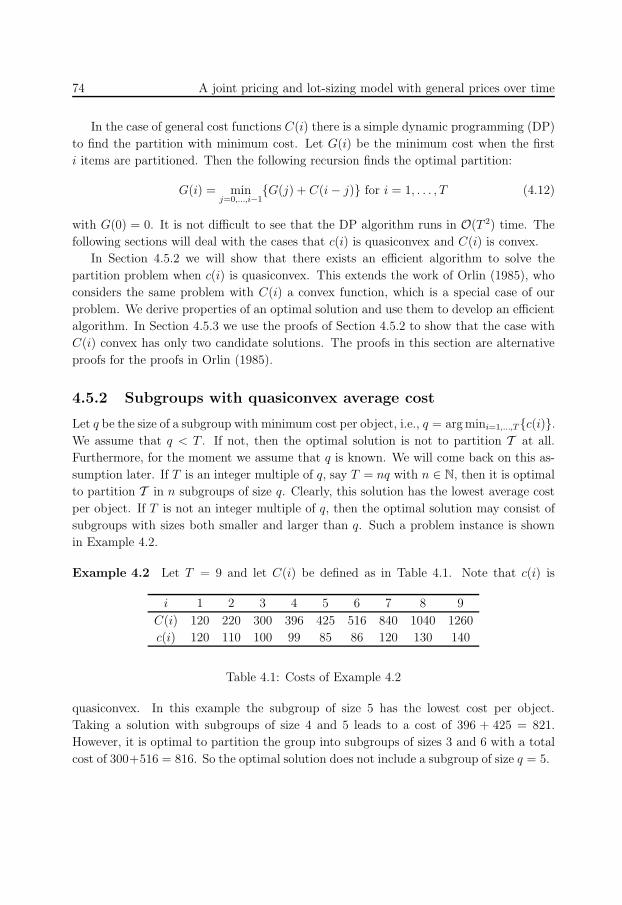
84

74 A joint pricing and lot-sizing model with general prices over time

In the case of general cost functions C(i) there is a simple dynamic programming (DP)

to find the partition with minimum cost. Let G(i) be the minimum cost when the first

i items are partitioned. Then the following recursion finds the optimal partition:

G(i) = minj=0,...,i−1

G(j) + C(i − j) for i = 1, . . . , T (4.12)

with G(0) = 0. It is not difficult to see that the DP algorithm runs in O(T 2) time. The

following sections will deal with the cases that c(i) is quasiconvex and C(i) is convex.

In Section 4.5.2 we will show that there exists an efficient algorithm to solve the

partition problem when c(i) is quasiconvex. This extends the work of Orlin (1985), who

considers the same problem with C(i) a convex function, which is a special case of our

problem. We derive properties of an optimal solution and use them to develop an efficient

algorithm. In Section 4.5.3 we use the proofs of Section 4.5.2 to show that the case with

C(i) convex has only two candidate solutions. The proofs in this section are alternative

proofs for the proofs in Orlin (1985).

4.5.2 Subgroups with quasiconvex average cost

Let q be the size of a subgroup with minimum cost per object, i.e., q = arg mini=1,...,Tc(i).We assume that q < T . If not, then the optimal solution is not to partition T at all.

Furthermore, for the moment we assume that q is known. We will come back on this as-

sumption later. If T is an integer multiple of q, say T = nq with n ∈ N, then it is optimal

to partition T in n subgroups of size q. Clearly, this solution has the lowest average cost

per object. If T is not an integer multiple of q, then the optimal solution may consist of

subgroups with sizes both smaller and larger than q. Such a problem instance is shown

in Example 4.2.

Example 4.2 Let T = 9 and let C(i) be defined as in Table 4.1. Note that c(i) is

i 1 2 3 4 5 6 7 8 9

C(i) 120 220 300 396 425 516 840 1040 1260

c(i) 120 110 100 99 85 86 120 130 140

Table 4.1: Costs of Example 4.2

quasiconvex. In this example the subgroup of size 5 has the lowest cost per object.

Taking a solution with subgroups of size 4 and 5 leads to a cost of 396 + 425 = 821.

However, it is optimal to partition the group into subgroups of sizes 3 and 6 with a total

cost of 300+516 = 816. So the optimal solution does not include a subgroup of size q = 5.

85

4.5 Intermezzo: A partition problem 75

Intuitively one may expect that the sizes of the subgroups do not deviate too much from

the optimal size q. The following two lemmas confirm this. We denote Li as the size of

subgroup i so that L1, . . . , Ln with∑n

i=1 Li = T represents a partition of T in n subgroups.

Lemma 4.3 Let L1, . . . , Ln be a partition of T and let I be the set with subgroups larger

than q, i.e., I = i : Li > q. Then∑

i∈I(Li − q) ≤ q − 1.

Proof Assume∑

i∈I(Li − q) ≥ q. Then we can decrease the sizes of the subgroups in I

such that each subgroup is of at least size q and we create a new subgroup of size q. Clearly,

we have a feasible solution and we have a decrease in average cost per object because the

sizes of the subgroups decrease (but are still larger than q) and c(i) is quasiconvex.

Lemma 4.4 Let L1, . . . , Lm be a partition of N and let I be the set with subgroups smaller

than q, i.e., I = i : Li < q. Then∑

i∈I(q − Li) ≤ q − 1.

Proof Assume∑

i∈I(q−Li) ≥ q. Let Lj be the smallest subgroup with j ∈ I. Construct a

new solution by adding the objects of Lj to the subgroups Li, such that Li ≤ q (i ∈ I\j).This is possible because

∑

i∈I

(q − Li) ≥ q ⇔ q − Lj +∑

i∈I\j

(q − Li) ≥ q ⇔ Lj ≤∑

i∈I\j

(q − Li).

Again, we have a decrease in cost because the average cost per object decreases and c(i)

is quasiconvex.

Lemmas 4.3 and 4.4 show that the sizes of the subgroups cannot deviate too much from q.

This helps us to develop an efficient procedure to find the optimal solution of the partition

problem.

Theorem 4.5 Let q be the size of subgroup with lowest cost per item. Then an optimal

solution of the partition problem can be found in a time that is polynomial in q.

Proof We only give the proof in case Li ≥ q for all i = 1, . . . , n. Similar arguments

can be used to prove the general case. Let I be the set of subgroups not equal to q, i.e.,

I = i : Li > q. We are interested in the total number of objects that may be contained

in subgroups larger than q. By definition of I this amount equals∑

i∈I Li. It can be

shown that the set I and the values of Li (i ∈ I) that maximize∑

i∈I Li and satisfy

Lemma 4.3, are Li = q + 1 and |I| = q − 1. So for an arbitrary solution it holds

∑

i∈I

Li ≤ (q − 1)(q + 1).

86

76 A joint pricing and lot-sizing model with general prices over time

This implies that at most (q − 1)(q + 1) objects may be partitioned into subgroups of

sizes larger than q and the remaining objects are partitioned into subgroups of size q.

Our solution procedure is now as follows. Let m = mini : T − qi ≤ (q − 1)(q + 1)(if (q − 1)(q + 1) ≥ T we set m = 0). Then we have at least m subgroups of size q in

the optimal solution. Now the remaining part of the problem, consisting of partitioning

T −mq ≤ (q − 1)(q + 1) objects, can be solved by the DP algorithm of Section 4.5.1 and

this takes no more than O(q4) time.

Note that the procedure in the proof is at least as fast as applying recursion (4.6). This

is because we have to apply recursion (4.6) to at most (q − 1)(q + 1) ≤ T periods.

4.5.3 Subgroups with convex cost

Orlin (1985) considers a special case of the problem and he assumes that C(i) is convex.

This is a stronger assumption, since C(i) is convex implies that c(i) is quasiconvex. In

the convex case we can even further speed up computations. In fact, we will show that

the optimal number of subgroups n can take on at most two values and we do not need

the DP approach. To show this we need the following lemmas.

Lemma 4.6 There exists an optimal partition for which |Li − Lj | ≤ 1 (i, j = 1, . . . , m).

Proof Let Li and Lj be subgroups with Li − Lj ≥ 2. Then moving one object from Li

to Lj does not lead to a cost increase since C(i) is convex. Repeating this procedure for

all Li and Lj with Li −Lj ≥ 2 leads to a solution with |Li −Lj | ≤ 1 and costs not larger

than the initial solution.

A direct consequence of Lemma 4.6 is that there exists an optimal solution where either

all subgroups have size at most q or size at least q. This is not necessarily true for the

case when c(i) is quasiconvex (see Example 4.2). The following theorem shows that in

case Li ≥ q for i = 1, . . . , n, the number of subgroups n is uniquely determined.

Theorem 4.7 If Li ≥ q for i = 1, . . . , n, then n =⌊

Tq

⌋.

Proof First, we have

T =n∑

i=1

Li ≥ nq ⇔ n ≤ T

q⇔ n ≤

⌊T

q

⌋,

87

4.6 Applying Orlin’s approach to the Bhattacharjee and Ramesh (2000) case 77

where the last equivalence follows from the integrality of n. Second, from Lemma 4.3 we

haven∑

i=1

(Li − q) ≤ q − 1 ⇔ T − nq ≤ q − 1

⇔ n ≥ T − (q − 1)

q

⇔ n ≥⌈

T − (q − 1)

q

⌉

⇔ n ≥⌊

T

q

⌋.

This implies that n =⌊

Tq

⌋.

Similarly to the proof of Theorem 4.7 we can prove Theorem 4.8.

Theorem 4.8 If Li ≤ q for i = 1, . . . , n, then n =⌈

nq

⌉.

It follows from Theorems 4.7 and 4.8 that⌊

T

q

⌋≤ n ≤

⌈T

q

⌉.

Furthermore, given n, the sizes of the subgroups are uniquely determined by Lemma 4.6.

Some algebra shows that we can only have subgroups of size t =⌊

Tn

⌋and size t + 1. To

be more precise, we have exactly n(t + 1) − T subgroups of size t and T − tn subgroups

of size t + 1. Note that if T is an integer multiple of q, then we have immediately found

the optimal partition.

As a final remark, we have assumed throughout this section that q is known (or can

be found by some analytical approach). If this is not the case, then q can be found by

searching for the smallest i that satisfies c(i + 1) − c(i) ≥ 0, which takes O(log T ) time.

4.6 Applying Orlin’s approach to the Bhattacharjee

and Ramesh (2000) case

Instead of solving the time-invariant joint pricing and lot-sizing problem with Thomas’

approach of Section 4.3, we can use the approach of the previous section (which we

will refer to as Orlin’s approach). Namely, given the values π1t, the pricing problem

is equivalent to the problem of partitioning the model horizon T into n subplans with

ti periods (i = 1, . . . , n) each with a profit π1ti , such that the total profit of the subplans∑ni=1 π1ti is maximized and

∑ni=1 ti = T . To apply the results of the previous section, we

need the following theorem.

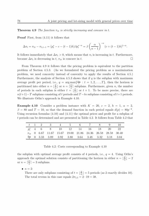
88

78 A joint pricing and lot-sizing model with general prices over time

Theorem 4.9 The function π1t is strictly increasing and concave in t.

Proof First, from (4.11) it follows that

∆πt = π1t − π1,t−1 = (p∗t − c − (t − 1)h)βp∗t−α = β

(α

α − 1

)−α

(c + (t − 1)h)1−α.

It follows immediately that ∆πt > 0, which means that πt is increasing in t. Furthermore,

because ∆πt is decreasing in t, π1t is concave in t.

From Theorem 4.9 it follows that the pricing problem is equivalent to the partition

problem of Section 4.5.3. (As we formulated the pricing problem as a maximization

problem, we need concavity instead of convexity to apply the results of Section 4.5.)

Furthermore, the analysis of Section 4.5.3 shows that if q is the subplan with maximum

average profit per period, i.e., q = arg maxπ1t

t: t = 1, 2, . . . , T, then the horizon is

partitioned into either n = ⌊Tq⌋ or n = ⌈T

q⌉ subplans. Furthermore, given n, the number

of periods in each subplan is either t = ⌊Tn⌋ or t + 1. To be more precise, there are

n(t+1)−T subplans consisting of t periods and T −tn subplans consisting of t+1 periods.

We illustrate Orlin’s approach in Example 4.10.

Example 4.10 Consider a problem instance with K = 20, c = 2, h = 1, α = 2,

β = 80 and T = 10, so that the demand function in each period equals d(p) = 80p−2.

Using recursion formulas (4.10) and (4.11) the optimal prices and profit for a subplan of

t periods can be determined and are presented in Table 4.2. It follows from Table 4.2 that

t 1 2 3 4 5 6 7 8 9 10

p∗t 4 6 8 10 12 14 16 18 20 22

π1t 0 6.67 11.67 15.67 19.00 21.86 24.36 26.58 28.58 30.40π1t

t0 3.33 3.89 3.92 3.80 3.64 3.48 3.32 3.18 3.04

Table 4.2: Costs corresponding to Example 4.10

the subplan with optimal average profit consists of 4 periods, i.e., q = 4. Using Orlin’s

approach the optimal solution consists of partitioning the horizon in either n = ⌊Tq⌋ = 2

or n = ⌈Tq⌉ = 3 subplans.

• n = 2:

There are only subplans consisting of t = ⌊Tn⌋ = 5 periods (as 2 exactly divides 10).

The total revenu in this case equals 2π1,5 = 2 · 19 = 38.

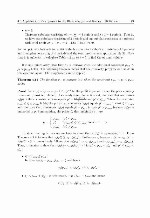
89

4.6 Applying Orlin’s approach to the Bhattacharjee and Ramesh (2000) case 79

• n = 3:

There are subplans consisting of t = ⌊Tn⌋ = 3 periods and t+1 = 4 periods. That is,

we have two subplans consisting of 3 periods and one subplan consisting of 4 periods

with total profit 2π1,3 + π1,4 = 2 · 11.67 + 15.67 ≈ 39.

So the optimal solution is to partition the horizon into 2 subplans consisting of 3 periods

and 1 subplan consisting of 4 periods and the total profit equals approximately 39. Note

that it is sufficient to calculate Table 4.2 up to t = 5 to find the optimal value q.

It is not immediately clear that π1t is concave when the additional constraint pmin ≤pt ≤ pmax holds. The following theorem shows that the concavity property still holds in

this case and again Orlin’s approach can be applied.

Theorem 4.11 The function π1t is concave in t when the constraint pmin ≤ pt ≤ pmax

holds.

Proof Let πi(p) = (p−c− (i−1)h)βp−α be the profit in period i when the price equals p

(where setup cost is excluded). As already shown in Section 4.4, the price that maximizes

πi(p) in the unconstrained case equals p∗i = α(c+(i−1)h)α−1

and p∗i < p∗i+1. When the constraint

pmin ≤ pt ≤ pmax holds, the price that maximizes πi(p) equals pi = pmin in case p∗i < pmin

and the price that maximizes πi(p) equals pi = pmax in case p∗i > pmax, because πi(p) is

unimodal in p. Summarizing, the prices pi that maximize π1t are

pi =

pmin if p∗i < pmin

p∗i if pmin ≤ p∗i ≤ pmax

pmax if p∗i > pmax

for i = 1, . . . , t.

To show that π1t is concave we have to show that πi(pi) is decreasing in i. From

Theorem 4.9 it follows that πi(p∗i ) ≥ πi+1(p

∗i+1). Furthermore, because πi(p) − πi+1(p) =

hβp−α > 0, it immediately follows that πi(pmin) > πi+1(pmin) and πi(pmax) > πi+1(pmax).

Thus, it remains to show that πi(pi)−πi+1(pi+1) ≥ 0 for p∗i < pmin ≤ p∗i+1 and p∗i ≤ pmax <

p∗i+1.

• p∗i < pmin ≤ p∗i+1:

In this case pi = pmin, pi+1 = p∗i and hence

πi(pmin) ≥ πi(p∗i+1) ≥ πi+1(p

∗i+1).

• p∗i ≤ pmax < p∗i+1: In this case pi = p∗i , pi+1 = pmax and hence

πi(p∗i ) ≥ πi+1(p

∗i+1) ≥ πi+1(pmax).

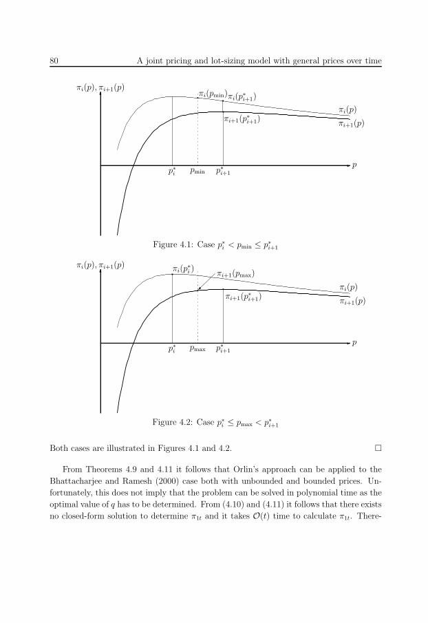
90

80 A joint pricing and lot-sizing model with general prices over time

6

-

πi(p), πi+1(p)

p∗i p∗i+1

p

πi(p)

pmin

πi(pmin)πi(p∗i+1)

πi+1(p∗i+1) πi+1(p)

Figure 4.1: Case p∗i < pmin ≤ p∗i+1

6

-

πi(p), πi+1(p)

p∗i p∗i+1

p

πi(p)

πi+1(p)

pmax

πi(p∗i )

πi+1(p∗i+1)

πi+1(pmax)

Figure 4.2: Case p∗i ≤ pmax < p∗i+1

Both cases are illustrated in Figures 4.1 and 4.2.

From Theorems 4.9 and 4.11 it follows that Orlin’s approach can be applied to the

Bhattacharjee and Ramesh (2000) case both with unbounded and bounded prices. Un-

fortunately, this does not imply that the problem can be solved in polynomial time as the

optimal value of q has to be determined. From (4.10) and (4.11) it follows that there exists

no closed-form solution to determine π1t and it takes O(t) time to calculate π1t. There-

91

4.6 Applying Orlin’s approach to the Bhattacharjee and Ramesh (2000) case 81

fore, finding q may take O(T ) time and hence Orlin’s approach has a pseudopolynomial

running time.

However, Orlin’s approach will be much faster in practice in case q ≪ T . Furthermore,

in case of other demand functions Orlin’s approach may be polynomial, whereas Thomas’

approach will be pseudopolynomial. For example, if we consider a simple linear demand

function, i.e.,

d(p) = β − αp,

then some algebra shows that the optimal price in period i of subplan 1, . . . , t equals

p∗i =1

2

(β

α+ c + (i − 1)h

)

and the optimal profit in period i equals

πi(p∗i ) =

1

2

(β

α− (c + (i − 1)h)

)2

.

This means that there exists a closed-form formula for π1t =∑t

i=1 πi(p∗i ) − K (since∑t

i=1 i2 = 16t(t + 1)(2t + 1)). Furthermore, it can be shown that π1t is concave in t.

Therefore, the optimal value q can be found by binary search and takes O(log T ) time.

This means that Orlin’s approach leads to a polynomial time algorithm (while Thomas’

approach does not).

In case the profit function π1t is quasiconcave, the value q can still be found by binary

search. If π1t can be calculated in constant time, this means that it takes again O(log T )

time to find q. Therefore, applying the solution approach in the proof of Theorem 4.5 will

be faster than applying Thomas’ approach. Finally, we note that Orlin’s approach and

the approach for the quasiconcave case become constant time algorithms when q is fixed

and given (in contrast to Thomas’ approach).

Bhattacharjee and Ramesh (2000) also consider the problem with perishable goods.

They assume that goods perish after m periods and hence they cannot be used anymore to

satisfy demand. Because of the time-invariant cost parameters the optimal solution still

consists of a series of consecutive subplans. Therefore, it is not optimal to have subplans

of more than m periods. In this case, again Orlin’s approach can be applied by setting

q := minq, m. (Note that subplans larger than m periods are not feasible in a solution.

The latter may occur when q = m and we have n = ⌊Tq⌋ subplans consisting of t = ⌈T

n⌉

and t + 1 periods. In this case the solution with n = ⌈Tq⌉ is optimal.)

Finally, we note that Orlin (1985) generalized a result by Chand (1982). Chand (1982)

also considers a partition problem in an ‘economic lot-sizing environment’. More specifi-

cally, he considers the ELS problem with time-invariant demand and cost parameters. In

this problem the costs of a subplan only depend on the number of periods in the subplan.

92

82 A joint pricing and lot-sizing model with general prices over time

Chand (1982) shows that there exists an optimal solution for which the number of periods

in any two subplans differ at most one period. Therefore, a similar approach as Orlin

(1985) can be applied to solve the problem. (The generalization of Orlin (1985) is that

lower and upper bounds are set on the number of periods in the subplan.)

4.7 Concerns about the results presented in Bhat-

tacharjee and Ramesh (2000)

Bhattacharjee and Ramesh (2000) proposed two heuristic algorithms to solve the joint

pricing and planning problem. To justify the application of heuristics, they refer to the

exponential nature of the problem and the characteristics of the maximum profit function.

Indeed there are 2T−1 possible production plans (assuming positive demand in period 1).

However, Thomas’ approach (see Section 4.3) circumvents this ‘exponentiality’ and the

problem can be solved to optimality by an efficient method. Note that the classical

Wagner-Whitin problem also has an exponential number of possible production plans,

but it can still be solved in polynomial time (Wagner and Whitin, 1958).

Furthermore, in both heuristics there is a predetermined value r, which defines the

maximum number of periods in a subplan to be considered. For such a subplan all (2r−1)

production plans are generated at the start of the algorithms. This does not only mean

that the heuristics have a running time which is exponential in r, but the heuristics

may also perform poorly if the optimal size of a subplan is larger than r. Bhattacharjee

and Ramesh (2000) report worst case deviations of more than 28% and 18% for the two

heuristics.

Besides the fact that the problem can be efficiently solved to optimality, Bhattacharjee

and Ramesh (2000) make several incorrect statements about the problem. Bhattacharjee

and Ramesh (2000, Theorem 1, p. 587) claim that for a profit-maximizing firm it is always

profitable to meet total demand. This means that shortage cost can be ignored and only

the model with no loss of demand needs to be considered. In the proof of this result the

authors use the fact that by increasing price in case of a shortage, there is an increase in

revenue and a saving in shortage cost. However, later they assume that pmin ≤ pt ≤ pmax,

which is a contradiction with the proof where it is assumed that price can always be

increased. In Example 4.12 we show that it can be optimal to have loss of demand.

Example 4.12 Consider a T -period example with K = 9, pmax − c = 3, pmin − c > 0,

s = 1 and h = 1, where s is the per unit shortage cost. Furthermore, let the demand

function be such that d(pmax) = 2 and (pmax−c)d(pmax) > (p−c)d(p) for all p < pmax. For

example, the function d(p) = 72p2 with pmin = 4, pmax = 6 and c = 3 satisfies this property.

Observe that

93

4.8 Conclusion 83

• it is not optimal to have both pt < pmax and unsatisfied demand in that period t

(see the argument used by Bhattacharjee and Ramesh (2000) in the “proof” of their

Theorem 1),

• it is not optimal to have pt < pmax and satisfy all demand in that period t (because

it is better to set the price to pmax and then satisfy all demand),

• it is not optimal to have pt = pmax and satisfy demand only partially in that period t

(because also satisfying the remainder of the demand will increase profit and lower

shortage costs).

It follows that in an optimal solution the price is set to pmax in every period and a period’s

demand is either completely satisfied or completely unsatisfied. One can easily verify that

for the parameter values given above only production runs that cover the complete demand

of two consecutive periods are profitable. A production run to cover only one period’s

demand is more expensive than leaving the demand unsatisfied. In case of three or more

periods, the holding costs of the third period are higher than the shortage costs. Hence,

the optimal solution is as follows. When T is even, there is a setup in every odd-numbered

period to satisfy completely the 4 units of demand of that and the next period. In case T

is odd, then there is exactly one (take any) odd-numbered period for which the 2 units of

demand are not satisfied. For the remaining periods the solution has the same structure

as in the case of an even number of periods.

4.8 Conclusion

In this chapter we considered a joint pricing and lot-sizing problem, where prices were

allowed to vary over time. We focused on a special case of this problem considered

by Bhattacharjee and Ramesh (2000) with a time-invariant demand function and time-

invariant cost parameters. We showed that a direct application of a method proposed by

Thomas (1970) led to an algorithm with a running time quadratic in the model horizon.

Moreover, applying the results on a partition problem derived by Orlin (1985) led to an

improvement in running time (although the running time was still pseudopolynomial).

By slightly generalizing the result of Orlin (1985), we showed that this result still holds

in case the profit function is quasiconcave in the number of periods of a subplan.

94

95

Chapter 5

A joint pricing and lot-sizing

problem with constant prices over

time∗

Abstract

In this chapter we consider the economic lot-size model, where demand is a de-

terministic function of price. In the model a single price needs to be set for all

periods. The objective is to find an optimal price and ordering decisions simulta-

neously. Kunreuther and Schrage (1973) proposed a heuristic algorithm to solve

this problem. The contribution of this chapter is twofold. First, we derive an exact

algorithm to determine the optimal price and lot-sizing decisions. Moreover, we

show that our algorithm boils down to solving a number of lot-sizing problems that

is quadratic in the number of periods, i.e., the problem can be solved in polynomial

time.

5.1 Introduction

In Chapter 4 we considered a joint pricing model where prices were allowed to vary over

time. There are several reasons why this may not be desirable. First, from Example 4.10

it can be seen that prices within a subplan (a consecutive number of periods for which

demand is covered by production in a single period) are strictly increasing over time. If

this happens in practice, customers may react on this and postpone purchases until the

price drops. In this case it may be desirable to set a constant price over all periods.

Second, as also mentioned in the general introduction, some firms rely on on sales from

∗This chapter is based on Van den Heuvel and Wagelmans (2006b).

96

86 A joint pricing and lot-sizing problem with constant prices over time

catalogues. It may be expensive to communicate price changes to customers and hence a

constant price over time is also desirable in this case.

In this chapter we consider a similar model as in Chapter 4 except that we assume a

constant price over time. In this chapter we build on the work of Kunreuther and Schrage

(1973) and Gilbert (1999). We propose an exact algorithm to solve the economic lot-sizing

(ELS) problem with deterministic demand functions and a constant price for all periods.

We propose an O(T 3 log T ) algorithm that solves the general problem as introduced by

Kunreuther and Schrage (1973). Furthermore, we show that our algorithm runs in O(T 2)

for the special case considered in Gilbert (1999).

The remainder of this chapter is organized as follows. In Section 5.2 we give a mathe-

matical formulation of the problem. In the next section we describe the heuristic algorithm

proposed by Kunreuther and Schrage (1973). In Section 5.4 we introduce an exact algo-

rithm which is an extension of the heuristic and we illustrate the algorithm by an example.

In Section 5.5 we analyze the time complexity of our algorithm and show that the running

time is polynomial in the number of periods. This chapter is ended up with a conclusion

and we give some suggestions for further research.

5.2 Problem description

First, we will describe the classical ELS problem in short. If we use the following notation

T : model horizon

Dt : demand in period t

Kt : setup costs in period t

ct : unit production costs in period t

ht : unit holding costs in period t

xt : production quantity in period t

It : ending inventory in period t,

then the problem can be formulated as

C(D) = min∑T

t=1 (Ktδ(xt) + ctxt + Itht)

s.t. It = It−1 − Dt + xt t = 1, . . . , T

xt, It ≥ 0, t = 1, . . . , T

I0 = 0

where

δ(x) =

0 for x = 0

1 for x > 0.

and D is the demand vector of length T . The first set of constraints models that the

ending inventory in period t equals the ending inventory in period t− 1 plus the amount

97

5.2 Problem description 87

produced in period t minus demand in period t. The second set of constraints models that

production and ending inventory are non-negative in each period. The above problem can

be solved efficiently by dynamic programming. Wagner and Whitin (1958) proposed an

O(T 2) algorithm to solve the problem. Federgruen and Tzur (1991), Wagelmans et al.

(1992) and Aggarwal and Park (1993) independently improved this result to O(T log T )

for the general case and to O(T ) for certain interesting cases, such as time-invariant cost

parameters.

Assume now that demand is not deterministic as in the ELS problem, but demand

is a deterministic function of the price and a single price for all periods needs to be set.

Kunreuther and Schrage (1973) propose the demand function

Dt(p) = αt + βtd(p),

where d(p) is a differentiable non-increasing function and αt, βt ≥ 0. This means that

demand will not increase, if the price increases. Note that the function d(p) is independent

of period t. If d(p) = −p we have a linear demand curve. Now the objective is not to

minimize the total costs as in the classical ELS problem, but to maximize total profit. If

we introduce the additional notation

Rt(p) = pDt(p), the revenue in period t,

then the objective can be formulated as

Π(D(p)) = maxp>0:D(p)≥0

T∑

t=1

Rt(p) − C(D(p))

,

where D(p) corresponds to the vector [D1(p), . . . , DT (p)].

Kunreuther and Schrage (1973) show that C(D(p)) is a concave piecewise linear func-

tion of the ‘demand effect’ d(p). This can be seen in the following way. Let S be the

set of production periods (in increasing order) of a production plan. Furthermore, let

s(i) be the first production period after period i and if period i has no successor, then

s(i) = T +1 by convention. Because of the zero-inventory property (Wagner and Whitin,

1958), a production plan is completely determined by its production periods. Now the

cost S(d(p)) of a production plan S equals

S(d(p)) =∑

i∈S

Ki +∑

i∈S

ci

s(i)−1∑

t=i

Dt(p) +T∑

i=1

s(i)−1∑

t=i+1

ht−1Di(p)

=∑

i∈S

Ki +∑

i∈S

ci

s(i)−1∑

t=i

(αt + βtd(p)) +

T∑

i=1

s(i)−1∑

t=i+1

ht−1(αi + βid(p)),

which shows that S(d(p)) is a linear function of d(p) for a fixed production plan S. Because

C(D(p)) is the lower envelope of linear functions and the number of possible production

98

88 A joint pricing and lot-sizing problem with constant prices over time

plans is finite, C(D(p)) is a concave piecewise linear function of d(p). This also means

that each line piece corresponds to a specific production plan S.

5.3 Heuristic algorithm

In this section we present the heuristic algorithm proposed by Kunreuther and Schrage

(1973). The algorithm works as follows:

1. Set i := 0, start with some initial price pi and set Πi := −∞.

2. Set i := i + 1.

3. Calculate the demand vector D(pi−1) and let Si be the optimal production plan

corresponding to problem C(D(pi−1))

4. Calculate the price pi which maximizes the net profit Πi :=∑T

t=1 Rt(pi)− Si(d(pi))

5. If Πi − Πi−1 > 0, then go to step 2.

6. The terminating price is pi with corresponding net profit Πi.

In the remainder of this chapter we will call this the KS-procedure. In step 3 of the

algorithm, we are looking for an optimal production plan given the demand vector D(pi−1),

which boils down to solving an instance of the ELS problem. In step 4 we are looking for

an optimal price corresponding to a fixed production plan. If we have a relatively easy

function d(p) (for instance, d(p) = −p), the optimization problem may be relatively easy

to solve (for instance,∑T

t=1 Rt(p) is quadratic for d(p) = −p). As in Kunreuther and

Schrage (1973) we assume that the optimization problem in step 3 can be solved (either

analytically or by a search procedure).

Kunreuther and Schrage (1973) show that the above algorithm does not skip over any

optimum on its way to the terminating price, i.e., if pi−1 and pi are two successive prices

generated by the KS-procedure, then∑T

t=1 Rt(pi)−C(D(pi)) ≥∑T

t=1 Rt(p)−S(d(p)) for

all prices p between pi−1 and pi and all plans S. Thus, if we have a lower bound pL and

an upper bound pU on the optimal price p∗ and we apply the KS-procedure with these

values as initial prices resulting in terminating prices p∗L and p∗U , respectively, then the

optimal price p∗ satisfies the inequality p∗L ≤ p∗ ≤ p∗U . So, if the terminating prices are

equal, we have found the optimal price.

A graphical representation of the algorithm is shown in figure 5.1. In the figure it is

assumed that d(p) = −p, so that∑T

t=1 Rt(p) is quadratic and C(D(p)) is a non-increasing

concave piecewise linear function of p. The derivatives of the revenue and cost function

are plotted against the price p. Because d(p) = −p, it follows immediately that the

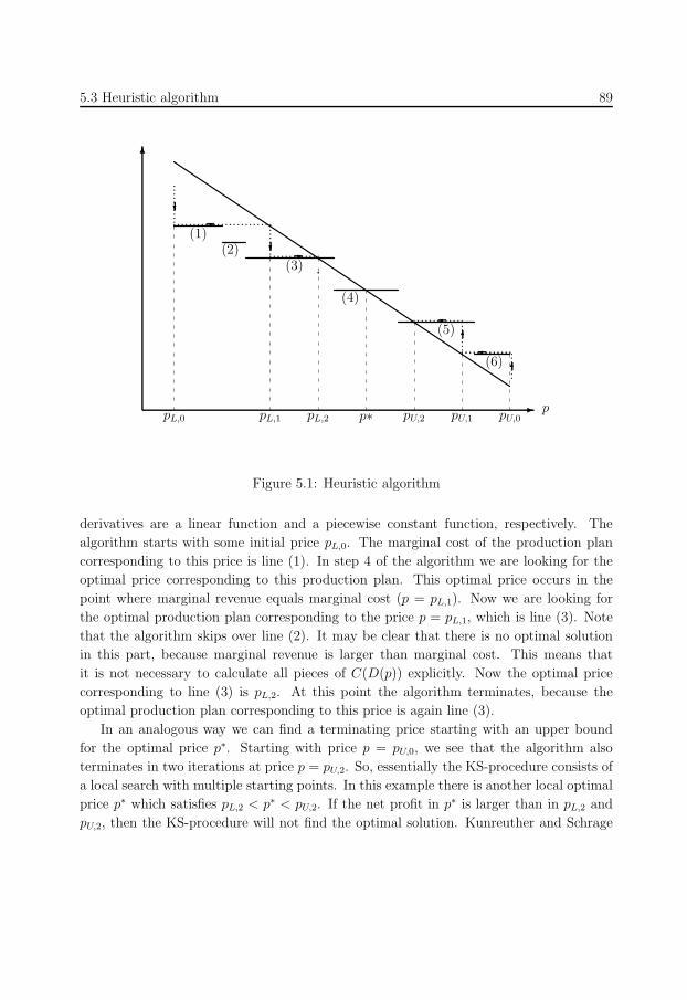
99

5.3 Heuristic algorithm 89

.............

......................... ......................

......................

..

.............

6

-pL,1 pL,2 p∗ pU,1pU,2

p

? -

6

-

pL,0 pU,0

(1)(2)

(3)

(4)

(5)

(6)

...........?

..

..

..

.

6

Figure 5.1: Heuristic algorithm

derivatives are a linear function and a piecewise constant function, respectively. The

algorithm starts with some initial price pL,0. The marginal cost of the production plan

corresponding to this price is line (1). In step 4 of the algorithm we are looking for the

optimal price corresponding to this production plan. This optimal price occurs in the

point where marginal revenue equals marginal cost (p = pL,1). Now we are looking for

the optimal production plan corresponding to the price p = pL,1, which is line (3). Note

that the algorithm skips over line (2). It may be clear that there is no optimal solution

in this part, because marginal revenue is larger than marginal cost. This means that

it is not necessary to calculate all pieces of C(D(p)) explicitly. Now the optimal price

corresponding to line (3) is pL,2. At this point the algorithm terminates, because the

optimal production plan corresponding to this price is again line (3).

In an analogous way we can find a terminating price starting with an upper bound

for the optimal price p∗. Starting with price p = pU,0, we see that the algorithm also

terminates in two iterations at price p = pU,2. So, essentially the KS-procedure consists of

a local search with multiple starting points. In this example there is another local optimal

price p∗ which satisfies pL,2 < p∗ < pU,2. If the net profit in p∗ is larger than in pL,2 and

pU,2, then the KS-procedure will not find the optimal solution. Kunreuther and Schrage

100

90 A joint pricing and lot-sizing problem with constant prices over time

(1973) give an example for which the algorithm does not converge. A slight modification

of that example shows that this may have major consequences for the net profit.

Example 5.1 Consider a three-period problem with K1 = 13.2, K2 = K3 = 10, ht =

h = 1, ct = c = 0 and Dt(p) = αt − βtd(p) with α1 = 25, α2 = α3 = 22, βt = β = 12

and d(p) = −p. If we start with pL,0 = 0, the algorithm terminates after one iteration

at pL,1 = 0.96 with net profit ΠL = −0.14. Starting with pU,0 = 2.08 (the largest price

for which demand is positive), the algorithm terminates after one iteration at pU,1 = 1.46

with net profit ΠU = −2.64. However, the optimal price equals p∗ = 1.13 with net profit

ΠU = 0.36 > ΠL > ΠU . This example shows that the KS-procedure may fail to find a

profitable solution if one does exist. In this case a firm may decide to not produce at all,

while it is profitable to produce. We will consider this problem instance in more detail

later. (Note: In this example all prices and profits have been rounded to nearest cent.)

5.4 Exact algorithm

In this section we present an exact algorithm to solve the ELS problem with deterministic

demand functions. The main idea of the exact algorithm is that the KS-procedure is

restarted. Assume that the heuristic algorithm starts with pL < pU and terminates with

prices p∗L and p∗U which satisfy pL ≤ p∗L < p∗U ≤ pU . To restart the algorithm we need a

suitable price p that satisfies p∗L < p < p∗U . In the exact algorithm we will find such a

price by applying an idea often attributed to Eisner and Severance (Eisner and Severance,

1976) on the function C(D(p)).

We will first explain how the Eisner Severance(ES)-method works. Assume we would

like to perform a parametric analysis on an optimization problem

z(λ) = min(c + λd)x

x ∈ X,

where X is a finite set. Here the vector of objective coefficients is a linear function of a

parameter λ. Assume we have some algorithm A to solve this optimization problem for

a fixed λ. It is well-known that the objective function z(λ) is a piecewise linear concave

function of λ. Assume that we want to find all breakpoints in the interval [λL, λU ]. This

can be done in the following way. Apply algorithm A on the optimization problem with

λ = λL and λ = λU . Calculate the intersection point λ of the lines corresponding to

λL and λU , say lL(λ) and lU(λ). Perform algorithm A on the optimization problem with

λ = λ. If the objective value is equal to lL(λ) and lU(λ), there is no new line piece between

λL and λU . Otherwise, apply the above procedure recursively with λL := λL and λU := λ

and with λL := λ and λU := λU .

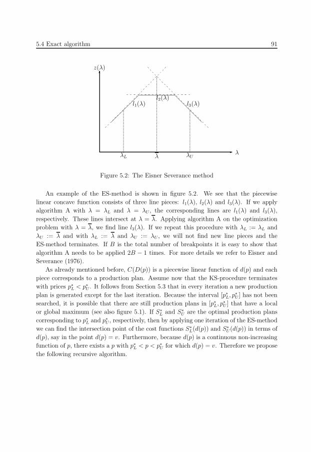
101

5.4 Exact algorithm 91

6

-

.............................

.............................

...................................................λL λUλ

l1(λ)l2(λ)

l3(λ)

z(λ)

λ

Figure 5.2: The Eisner Severance method

An example of the ES-method is shown in figure 5.2. We see that the piecewise

linear concave function consists of three line pieces: l1(λ), l2(λ) and l3(λ). If we apply

algorithm A with λ = λL and λ = λU , the corresponding lines are l1(λ) and l3(λ),

respectively. These lines intersect at λ = λ. Applying algorithm A on the optimization

problem with λ = λ, we find line l3(λ). If we repeat this procedure with λL := λL and

λU := λ and with λL := λ and λU := λU , we will not find new line pieces and the

ES-method terminates. If B is the total number of breakpoints it is easy to show that

algorithm A needs to be applied 2B − 1 times. For more details we refer to Eisner and

Severance (1976).

As already mentioned before, C(D(p)) is a piecewise linear function of d(p) and each

piece corresponds to a production plan. Assume now that the KS-procedure terminates

with prices p∗L < p∗U . It follows from Section 5.3 that in every iteration a new production

plan is generated except for the last iteration. Because the interval [p∗L, p∗U ] has not been

searched, it is possible that there are still production plans in [p∗L, p∗U ] that have a local

or global maximum (see also figure 5.1). If S∗L and S∗

U are the optimal production plans

corresponding to p∗L and p∗U , respectively, then by applying one iteration of the ES-method

we can find the intersection point of the cost functions S∗L(d(p)) and S∗

U(d(p)) in terms of

d(p), say in the point d(p) = v. Furthermore, because d(p) is a continuous non-increasing

function of p, there exists a p with p∗L < p < p∗U for which d(p) = v. Therefore we propose

the following recursive algorithm.

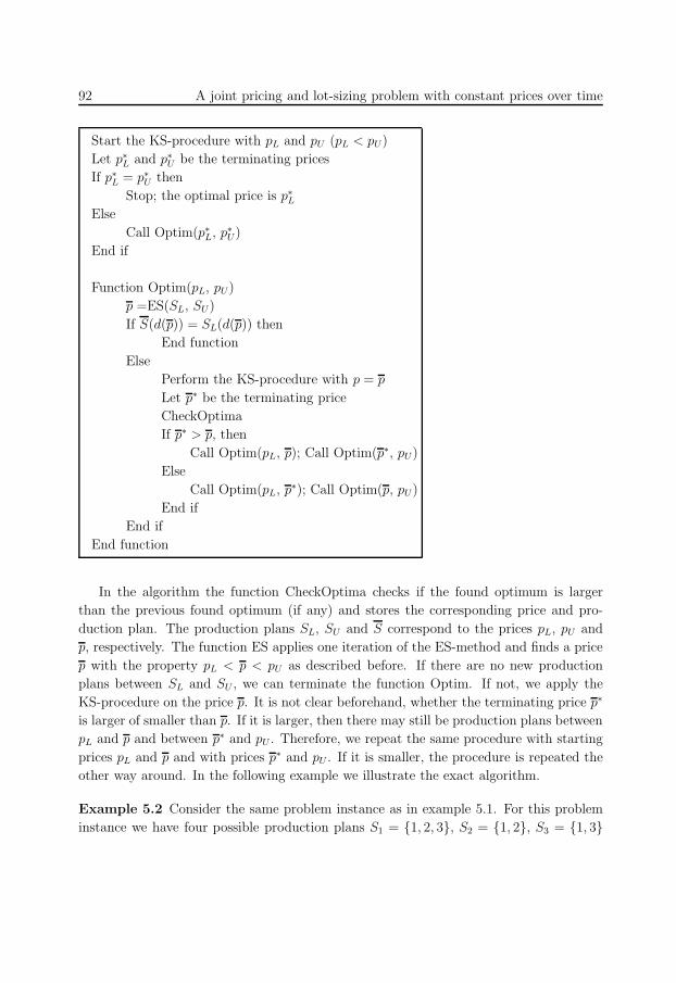
102

92 A joint pricing and lot-sizing problem with constant prices over time

Start the KS-procedure with pL and pU (pL < pU)

Let p∗L and p∗U be the terminating prices

If p∗L = p∗U then

Stop; the optimal price is p∗LElse

Call Optim(p∗L, p∗U)

End if

Function Optim(pL, pU)

p =ES(SL, SU)

If S(d(p)) = SL(d(p)) then

End function

Else

Perform the KS-procedure with p = p

Let p∗ be the terminating price

CheckOptima

If p∗ > p, then

Call Optim(pL, p); Call Optim(p∗, pU)

Else

Call Optim(pL, p∗); Call Optim(p, pU)

End if

End if

End function

In the algorithm the function CheckOptima checks if the found optimum is larger

than the previous found optimum (if any) and stores the corresponding price and pro-

duction plan. The production plans SL, SU and S correspond to the prices pL, pU and

p, respectively. The function ES applies one iteration of the ES-method and finds a price

p with the property pL < p < pU as described before. If there are no new production

plans between SL and SU , we can terminate the function Optim. If not, we apply the

KS-procedure on the price p. It is not clear beforehand, whether the terminating price p∗

is larger of smaller than p. If it is larger, then there may still be production plans between

pL and p and between p∗ and pU . Therefore, we repeat the same procedure with starting

prices pL and p and with prices p∗ and pU . If it is smaller, the procedure is repeated the

other way around. In the following example we illustrate the exact algorithm.

Example 5.2 Consider the same problem instance as in example 5.1. For this problem

instance we have four possible production plans S1 = 1, 2, 3, S2 = 1, 2, S3 = 1, 3

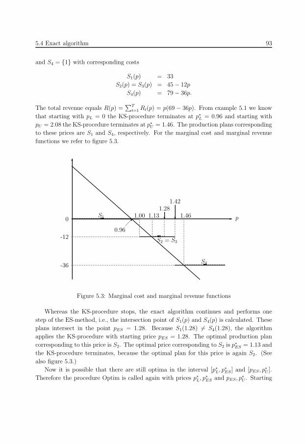
103

5.4 Exact algorithm 93

and S4 = 1 with corresponding costs

S1(p) = 33

S2(p) = S3(p) = 45 − 12p

S4(p) = 79 − 36p.

The total revenue equals R(p) =∑T

t=1 Rt(p) = p(69 − 36p). From example 5.1 we know

that starting with pL = 0 the KS-procedure terminates at p∗L = 0.96 and starting with

pU = 2.08 the KS-procedure terminates at p∗U = 1.46. The production plans corresponding

to these prices are S1 and S4, respectively. For the marginal cost and marginal revenue

functions we refer to figure 5.3.

6

- p

.......................................

...........................................................

-12

-36 ...........................

..

..

..

..

..

.

..

..

..

..

..

.

..

..

..

..

..

. 1.46

1.42

1.00

0.96

?1.13 ...........

1.28

?0 ..................................

.......

.......................

-

S1

S2 = S3

S4

Figure 5.3: Marginal cost and marginal revenue functions

Whereas the KS-procedure stops, the exact algorithm continues and performs one

step of the ES-method, i.e., the intersection point of S1(p) and S4(p) is calculated. These

plans intersect in the point pES = 1.28. Because S1(1.28) 6= S4(1.28), the algorithm

applies the KS-procedure with starting price pES = 1.28. The optimal production plan

corresponding to this price is S2. The optimal price corresponding to S2 is p∗ES = 1.13 and

the KS-procedure terminates, because the optimal plan for this price is again S2. (See

also figure 5.3.)

Now it is possible that there are still optima in the interval [p∗L, p∗ES] and [pES, p∗U ].

Therefore the procedure Optim is called again with prices p∗L, p∗ES and pES, p∗U . Starting

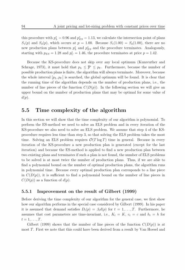
104

94 A joint pricing and lot-sizing problem with constant prices over time

this procedure with p∗L = 0.96 and p∗ES = 1.13, we calculate the intersection point of plans

S1(p) and S2(p), which occurs at p = 1.00. Because S1(1.00) = S2(1.00), there are no

new production plans between p∗L and p∗ES and the procedure terminates. Analogously,

starting with pES = 1.28 and p∗U = 1.46, the procedure terminates at price p = 1.42.

Because the KS-procedure does not skip over any local optimum (Kunreuther and

Schrage, 1973), it must hold that pL ≤ p∗ ≤ pU . Furthermore, because the number of

possible production plans is finite, the algorithm will always terminate. Moreover, because

the whole interval [pL, pU ] is searched, the global optimum will be found. It is clear that

the running time of the algorithm depends on the number of production plans, i.e., the

number of line pieces of the function C(D(p)). In the following section we will give an

upper bound on the number of production plans that may be optimal for some value of

d(p).

5.5 Time complexity of the algorithm

In this section we will show that the time complexity of our algorithm is polynomial. To

perform the ES-method we need to solve an ELS problem and in every iteration of the

KS-procedure we also need to solve an ELS problem. We assume that step 4 of the KS-

procedure requires less time than step 3, so that solving the ELS problem takes the most

time. Solving an ELS problem requires O(T log T ) time in general. Because in every

iteration of the KS-procedure a new production plan is generated (except for the last

iteration) and because the ES-method is applied to find a new production plan between

two existing plans and terminates if such a plan is not found, the number of ELS problems

to be solved is at most twice the number of production plans. Thus, if we are able to

find a polynomial bound on the number of optimal production plans, the algorithm runs

in polynomial time. Because every optimal production plan corresponds to a line piece

in C(D(p)), it is sufficient to find a polynomial bound on the number of line pieces in

C(D(p)) as a function of d(p).

5.5.1 Improvement on the result of Gilbert (1999)

Before deriving the time complexity of our algorithm for the general case, we first show

how our algorithm performs in the special case considered by Gilbert (1999). In his paper

it is assumed that demand satisfies Dt(p) = βtd(p) for t = 1, . . . , T . Furthermore, he

assumes that cost parameters are time-invariant, i.e., Kt = K, ct = c and ht = h for

t = 1, . . . , T .

Gilbert (1999) shows that the number of line pieces of the function C(D(p)) is at

most T . First we note that this could have been derived from a result by Van Hoesel and

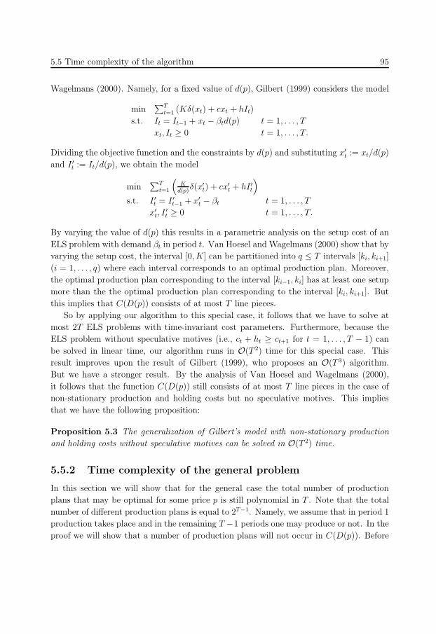
105

5.5 Time complexity of the algorithm 95

Wagelmans (2000). Namely, for a fixed value of d(p), Gilbert (1999) considers the model

min∑T

t=1 (Kδ(xt) + cxt + hIt)

s.t. It = It−1 + xt − βtd(p) t = 1, . . . , T

xt, It ≥ 0 t = 1, . . . , T.

Dividing the objective function and the constraints by d(p) and substituting x′t := xt/d(p)

and I ′t := It/d(p), we obtain the model

min∑T

t=1

(K

d(p)δ(x′

t) + cx′t + hI ′

t

)

s.t. I ′t = I ′

t−1 + x′t − βt t = 1, . . . , T

x′t, I

′t ≥ 0 t = 1, . . . , T.

By varying the value of d(p) this results in a parametric analysis on the setup cost of an

ELS problem with demand βt in period t. Van Hoesel and Wagelmans (2000) show that by

varying the setup cost, the interval [0, K] can be partitioned into q ≤ T intervals [ki, ki+1]

(i = 1, . . . , q) where each interval corresponds to an optimal production plan. Moreover,

the optimal production plan corresponding to the interval [ki−1, ki] has at least one setup

more than the the optimal production plan corresponding to the interval [ki, ki+1]. But

this implies that C(D(p)) consists of at most T line pieces.

So by applying our algorithm to this special case, it follows that we have to solve at

most 2T ELS problems with time-invariant cost parameters. Furthermore, because the

ELS problem without speculative motives (i.e., ct + ht ≥ ct+1 for t = 1, . . . , T − 1) can

be solved in linear time, our algorithm runs in O(T 2) time for this special case. This

result improves upon the result of Gilbert (1999), who proposes an O(T 3) algorithm.

But we have a stronger result. By the analysis of Van Hoesel and Wagelmans (2000),

it follows that the function C(D(p)) still consists of at most T line pieces in the case of

non-stationary production and holding costs but no speculative motives. This implies

that we have the following proposition:

Proposition 5.3 The generalization of Gilbert’s model with non-stationary production

and holding costs without speculative motives can be solved in O(T 2) time.

5.5.2 Time complexity of the general problem

In this section we will show that for the general case the total number of production

plans that may be optimal for some price p is still polynomial in T . Note that the total

number of different production plans is equal to 2T−1. Namely, we assume that in period 1

production takes place and in the remaining T −1 periods one may produce or not. In the

proof we will show that a number of production plans will not occur in C(D(p)). Before

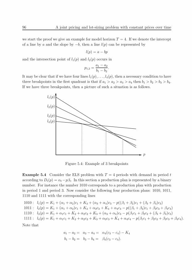
106

96 A joint pricing and lot-sizing problem with constant prices over time

we start the proof we give an example for model horizon T = 4. If we denote the intercept

of a line by a and the slope by −b, then a line l(p) can be represented by

l(p) = a − bp

and the intersection point of l1(p) and l2(p) occurs in

p1,2 =a1 − a2

b1 − b2.

It may be clear that if we have four lines l1(p), . . . , l4(p), then a necessary condition to have

three breakpoints in the first quadrant is that if a1 > a2 > a3 > a4 then b1 > b2 > b3 > b4.

If we have three breakpoints, then a picture of such a situation is as follows.

6

-..................................

...

...

...

...

...

...

...

...

..

...

...

...

...

...

..

l1(p)

l2(p)

l3(p)

l4(p)

p

Figure 5.4: Example of 3 breakpoints

Example 5.4 Consider the ELS problem with T = 4 periods with demand in period t

according to Dt(p) = αt−pβt. In this section a production plan is represented by a binary

number. For instance the number 1010 corresponds to a production plan with production

in period 1 and period 3. Now consider the following four production plans: 1010, 1011,

1110 and 1111 with the corresponding lines

1010 : l1(p) = K1 + (α1 + α2)c1 + K3 + (α3 + α4)c3 − p((β1 + β2)c1 + (β3 + β4)c3)

1011 : l2(p) = K1 + (α1 + α2)c1 + K3 + α3c3 + K4 + α4c4 − p((β1 + β2)c1 + β3c3 + β4c4)

1110 : l3(p) = K1 + α1c1 + K2 + α2c2 + K3 + (α3 + α4)c3 − p(β1c1 + β2c2 + (β3 + β4)c3)

1111 : l4(p) = K1 + α1c1 + K2 + α2c2 + K3 + α3c3 + K4 + α4c4 − p(β1c1 + β2c2 + β3c3 + β4c4).

Note that

a1 − a2 = a3 − a4 = α4(c3 − c4) − K4

b1 − b2 = b3 − b4 = β4(c3 − c4).

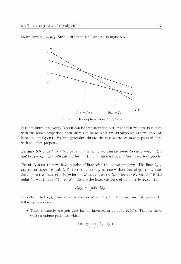
107

5.5 Time complexity of the algorithm 97

So we have p1,2 = p3,4. Such a situation is illustrated in figure 5.5.

6

-

a1

a2

a3

a4

...

...

...

...

...

...

...

...

...

...

...

...

...

...

..

...

...

...

...

...

...

...

...

...

...

...

p1,2 = p3,4 p1,3 = p2,4p

Figure 5.5: Example with a1 > a2 > a3

It is not difficult to verify (and it can be seen from the picture) that if we have four lines

with the above properties, then there can be at most two breakpoints and we ‘lose’ at

least one breakpoint. We can generalize this to the case where we have n pairs of lines

with this nice property.

Lemma 5.5 If we have n ≥ 2 pairs of lines l1, . . . , l2n with the properties a2i−1−a2i = a

and b2i−1 − b2i = b with b 6= 0 for i = 1, . . . , n, then we lose at least n− 1 breakpoints.

Proof Assume that we have n pairs of lines with the above property. The lines l2i−1

and l2i correspond to pair i. Furthermore, we may assume without loss of generality that

b > 0, so that l2i−1(p) > l2i(p) for p < p∗ and l2i−1(p) < l2i(p) for p > p∗, where p∗ is the

point for which l2i−1(p∗) = l2i(p

∗). Denote the lower envelope of the lines by Fn(p), i.e.,

Fn(p) = mini=1,...,2n

li(p).

It is clear that Fn(p) has a breakpoint in p∗ = a/b. Now we can distinguish the

following two cases.

• There is exactly one pair that has an intersection point in Fn(p∗). That is, there

exists a unique pair i for which

i = arg minj=1,...,n

l2j−1(p∗).

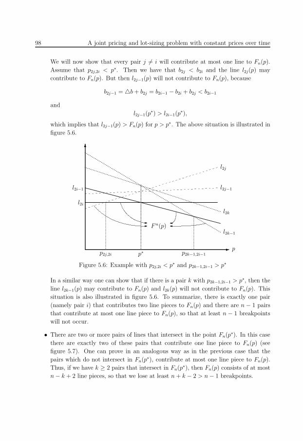
108

98 A joint pricing and lot-sizing problem with constant prices over time

We will now show that every pair j 6= i will contribute at most one line to Fn(p).

Assume that p2j,2i < p∗. Then we have that b2j < b2i and the line l2j(p) may

contribute to Fn(p). But then l2j−1(p) will not contribute to Fn(p), because

b2j−1 = b + b2j = b2i−1 − b2i + b2j < b2i−1

and

l2j−1(p∗) > l2i−1(p

∗),

which implies that l2j−1(p) > Fn(p) for p > p∗. The above situation is illustrated in

figure 5.6.

6

-

..........

..........

..........

..........

..........

..........

..........

..........

..........

..........

........

..................................................................................................

p2k−1,2i−1

...

...

...

...

...

...

...

..

l2i−1

l2i

................................................

...

...

...

...

...

...

...

...

...

...

...

...

...

...

.................................p∗p2j,2i

l2j−1

l2j

l2k−1

l2k

p

F n(p)--

Figure 5.6: Example with p2j,2i < p∗ and p2k−1,2i−1 > p∗

In a similar way one can show that if there is a pair k with p2k−1,2i−1 > p∗, then the

line l2k−1(p) may contribute to Fn(p) and l2k(p) will not contribute to Fn(p). This

situation is also illustrated in figure 5.6. To summarize, there is exactly one pair

(namely pair i) that contributes two line pieces to Fn(p) and there are n − 1 pairs

that contribute at most one line piece to Fn(p), so that at least n − 1 breakpoints

will not occur.

• There are two or more pairs of lines that intersect in the point Fn(p∗). In this case

there are exactly two of these pairs that contribute one line piece to Fn(p) (see

figure 5.7). One can prove in an analogous way as in the previous case that the

pairs which do not intersect in Fn(p∗), contribute at most one line piece to Fn(p).

Thus, if we have k ≥ 2 pairs that intersect in Fn(p∗), then Fn(p) consists of at most

n − k + 2 line pieces, so that we lose at least n + k − 2 > n − 1 breakpoints.

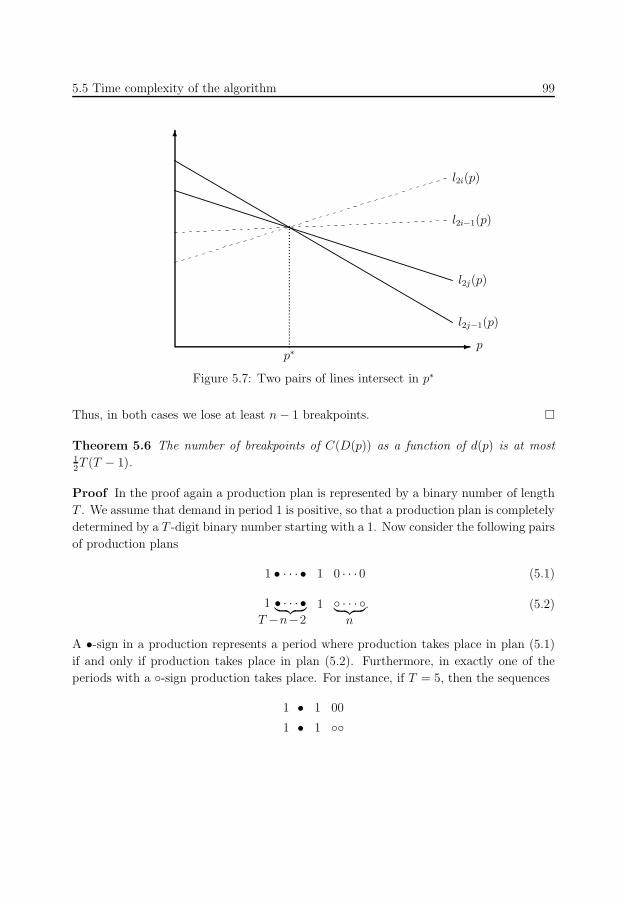
109

5.5 Time complexity of the algorithm 99

6

-.........................................

l2i−1(p)

l2i(p)

l2j−1(p)

l2j(p)

pp∗

Figure 5.7: Two pairs of lines intersect in p∗

Thus, in both cases we lose at least n − 1 breakpoints.

Theorem 5.6 The number of breakpoints of C(D(p)) as a function of d(p) is at most12T (T − 1).

Proof In the proof again a production plan is represented by a binary number of length

T . We assume that demand in period 1 is positive, so that a production plan is completely

determined by a T -digit binary number starting with a 1. Now consider the following pairs

of production plans

1 • · · · • 1 0 · · · 0 (5.1)

1 • · · · •︸ ︷︷ ︸T −n−2

1 · · · ︸ ︷︷ ︸n

. (5.2)

A •-sign in a production represents a period where production takes place in plan (5.1)

if and only if production takes place in plan (5.2). Furthermore, in exactly one of the

periods with a -sign production takes place. For instance, if T = 5, then the sequences

1 • 1 00

1 • 1

110

100 A joint pricing and lot-sizing problem with constant prices over time

represent two times two pairs of production plans

10100 10100

10101 10110

11100 11100

11101 11110.

We will now show that production pairs with identical ‘tails’ satisfy the properties of

Lemma 5.5. Let S be the set of production periods (in increasing order) for a production

plan. For instance with T = 5 the production plan 10101 corresponds to S = 1, 3, 5.Furthermore, if i is an production period, then s(i) is the successive production period

and the successor of the last production period equals T +1 by convention. Now the cost

S(d(p)) of a production plan S as a function of d(p) equals

S(d(p)) =∑

i∈S

Ki + ci

s(i)−1∑

t=i

Dt(p)

=∑

i∈S

Ki + ci

s(i)−1∑

t=i

αt

− d(p)∑

i∈S

ci

s(i)−1∑

t=i

βt.

(5.3)

Note that there are no holding costs in (5.3). It can be shown (see for example Wagelmans

et al. (1992)) that every ELS problem can be rewritten as an ELS problem without holding

cost by making the substitution ct := ct +∑T

i=t ht.

Assume now that we have a pair of production plans S1 and S2 according to (5.1)

and (5.2), respectively, with period m and n (m < n) corresponding to the one but last

and last production period in S2, i.e., S1 = i1, . . . , ik, m and S2 = i1, . . . , ik, m, n. It

follows from (5.3) that

S2(d(p)) − S1(d(p)) = Kn + (cn − cm)T∑

t=T−n+1

αt + p(cm − cn)T∑

t=T−n+1

βt. (5.4)

It follows immediately from (5.4) that the difference in intercept and slope is independent

of the sequence i1, . . . , ik.

Now for a fixed n ≥ 1 and a fixed production period in the last n periods, there

are T − n − 2 positions for the •-sign, implying that we have 2T−n−2 pairs with the

properties of Lemma 5.5. It follows from this lemma that we lose 2T−n−2 −1 breakpoints.

Because we have n possible positions for the -sign and n ranges from 1 to T − 3, we lose∑T−3n=1 n(2T−n−2 −1) breakpoints in total. Furthermore, because the maximum number of

breakpoints for model horizon T equals 2T−1 − 1, the maximum number of breakpoints

111

5.5 Time complexity of the algorithm 101

equals

2T−1 − 1 −T−3∑

n=1

n(2T−n−2 − 1) =

2T−1 − 1 +1

2(T − 3)(T − 2) −

T−3∑

n=1

n2T−n−2 =

2T−1 − 1 +1

2(T − 3)(T − 2) − (−2(T − 1) + 2T−1) =

1

2T (T − 1),

where the second equality follows from Lemma 5.7 (see appendix 5.A).

As it follows from example 5.4 and figure 5.5, if li(p), lj(p) and lm(p), ln(p) are pairs of

lines with the properties of Lemma 5.5, then the pairs li(p), lm(p) and lj(p), lj(p) also have

these properties. Call these pairs the complement pairs. Thus, to complete the proof we

have to check that none of the pairs defined in (5.1) and (5.2) are complement pairs of

each other. To see that this holds, note that the tails of the complement pairs (i.e., the

production periods of the last n + 1 periods) are identical for pairs constructed according

to (5.1) and (5.2) with n fixed. However, the tails of the production pairs defined in (5.1)

and (5.2) are different. This means that the pairs can never be complement pairs of each

other.

So using the result of Theorem 5.6 and noting that the ELS problem can be solved in

O(T log T ) time, it follows that our algorithm has a time complexity of O(T 3 log T ).

5.5.3 An Ω(T 2) example

In this section we show that the bound on the number of optimal production plans in

C(D(p)) in Section 5.5.2 is tight. Consider the following problem instance. Let

Dt(p) = D − p for t = 1, . . . , T

Kt = (T − t + 1)K for t = 1, . . . , T

ct = T T−t+1 for t = 1, . . . , T

ht = 0 for t = 1, . . . , T.

Again production plans are represented by binary numbers. We construct production

plans in the following way. We start with a production plan with only a setup in period 1.

The next production plan is constructed by adding a setup in period T and the following

production plans are constructed by moving this setup one period earlier. If this is not

possible anymore, we start the procedure again by adding a setup in period T . Formally,

if

Si = 1 • · · · • 010 · · ·0

112

102 A joint pricing and lot-sizing problem with constant prices over time

is a production plan, then

Si+1 = 1 • · · · • 100 · · ·0is the next production plan, where • · · · • is the same sequence in both plans, and if

Sj = 1 · · ·10 · · ·00

is a production plan, then

Sj+1 = 1 · · ·10 · · ·01

is the successive production plan. We will call this the ‘in’-plans. For instance, the

in-plans corresponding to T = 4 are 1000, 1001, 1010, 1100, 1101, 1110, 1111.

The main idea of the proof is as follows. If we only consider the in-plans, we will show

that these plans all contribute to the lower envelope. Then, if we consider the remaining

production plans, the ‘out’-plans (for instance, 1011 is an out-plan for T = 4), we will

show that they will not contribute to the lower envelope. Therefore, we will first show

some properties of the production plans. Note that we can construct all production plans

by binary counting, starting with the number 10 · · ·0 and ending with 11 · · ·1.

The first property is that the slopes of all plans are decreasing. Let S1 be a production

plan and S2 be the successive production plan. Furthermore, let k ≤ T be the last non-

production period and n be the first production period before k of plan S1 (see the

following picture).

n k

S1 = 1 • · · · • 10 · · ·0 01 · · ·1S2 = 1 • · · · • 10 · · ·0 10 · · ·0

If we denote the (negative) slope b(Si) of plan Si by

b(Si) =∑

i∈Si

ci

s(i)−1∑

t=i

1,

then we have that

b(S1) − b(S2) = (5.5)

∑

i∈S1

ci

s(i)−1∑

t=i

1 −∑

i∈S2

ci

s(i)−1∑

t=i

1 = (5.6)

cn +

T∑

t=k+1

ct − ck(T − k + 1) ≥ (5.7)

T · T T−k+1 +T∑

t=k+1

T T−k+1 − (T − k + 1)T T−k+1 ≥ (5.8)

T∑

t=k+1

T T−k+1 > 0. (5.9)

113

5.5 Time complexity of the algorithm 103

Note that the third inequality holds, because n ≤ k−1 which implies that cn ≥ ck−1 = Tck

and the last inequality holds because k ≥ 2 so that T − 1 ≥ T − k + 1.

If K is sufficiently small, then we can show that the intercepts of the production plans

(constructed by binary counting) are also decreasing. Recall that the intercept a(Si) of

production plan equals

a(Si) =∑

i∈Si

Ki + ci

s(i)−1∑

t=i

αt

.

If we neglect the term∑

i∈SiKi and because demand is constant, we have

a(Si) =∑

i∈Si

ci

s(i)−1∑

t=i

D = Db(Si).

Because b(Si) is decreasing for consecutive plans Si, it is clear that the intercepts a(Si)

are also decreasing.

For the intercepts of the in-plans we can prove a stronger result. Namely, the difference

between the slopes of consecutive plans are decreasing, i.e., b(Si) − b(Si+1) > b(Si+1) −b(Si+2). If Si, Si+1 and Si+2 are of the following structure

n k

Si = 1 · · ·1 0 · · ·000 10 · · ·0Si+1 = 1 · · ·1 0 · · ·001 00 · · ·0Si+2 = 1 · · ·1 0 · · ·010 00 · · ·0,

(5.10)

then it holds that

b(Si) − b(Si+1) = cn − (T − k + 1)ck + (T − k + 2)ck−1

and

b(Si) − 2b(Si+1) + b(Si+2) = (T − k + 3)T 2 − 2(T − k + 2)T + (T − k + 1) > 0

for T ≥ 1 and T − k + 1 ≥ 0, so that b(Si) − b(Si+1) > b(Si+1) − b(Si+2). For other

consecutive in-plans one can obtain the same result.

Now we consider the intersection points of two plans S1 and S2. It follows from 5.3

that if S1(p) = S2(p), then

pS1,S2= D +

∑i∈S1

Ki −∑

i∈S2Ki

b(S1) − b(S2). (5.11)

Consider two consecutive in-plans Si and Si+1. If we have a transition from plan Si to

Si+1 according to (5.10), then we have∑

j∈Si

Kj −∑

j∈Si+1

Kj = Kk − Kk−1 = (T − k + 1)K − (T − (k − 1) + 1)K = −K

114

104 A joint pricing and lot-sizing problem with constant prices over time

and if we have a transition according to

Si = 1 · · ·10 · · ·00

Si+1 = 1 · · ·10 · · ·01,(5.12)

then ∑

j∈Si

Kj −∑

j∈Si+1

Kj = −KT = −K.

This means that∑

j∈SiKj −

∑j∈Si+1

Kj is constant. Because b(Si)−b(Si+1) is decreasing,

it follows from (5.11) that the intersection points are decreasing, which implies that all

in-plans contribute to the lower envelope.

We will now show that the out-plans will not contribute to the lower envelope. There-

fore, consider the following production plans

n k

Si = 1 · · ·1 0 · · ·00 10 · · ·0Si+1 = 1 · · ·1 0 · · ·00 1 · · · Si+2 = 1 · · ·1 0 · · ·01 00 · · ·0,

(5.13)

where Si+1 is a plan with at least one setup in the period(s) with a -sign. Thus, Si is

an in-plan with Si+2 as a successor and Si+1 is an out-plan. To show that Si+1 does not

contribute to the lower envelop, it is sufficient to show that pSi+1,Si+2> pSi,Si+2

. We have

that ∑

i∈Si+1

Ki ≥∑

i∈Si

Ki + Km ≥∑

i∈Si+2

Ki,

because Kk + Km ≥ Kk−1, where m (k < m ≤ T ) is a setup period in Si+1. But then it

follows from (5.11) that

pSi,Si+2< D ≤ pSi+1,Si+2

.

Because all out-plans have the same structure as Si+1 in (5.13), only the in-plans con-

tribute to the lower envelope.

To count the number of breakpoints of the lower envelope, we have to count the number

of in-plans. We have exactly one in-plan with a setup in period 1, T − 1 in-plans with 2

setups, T − 2 in-plans with 3 setups, etc. This means that the total number of line pieces

equals

1 +T−1∑

t=1

t = 1 +1

2T (T − 1)

and the number of breakpoints equals 12T (T − 1).

115

5.6 Concluding remarks 105

5.6 Concluding remarks

In this chapter we have presented an exact algorithm to solve the ELS problem with deter-

ministic demand functions. We improved the heuristic algorithm proposed by Kunreuther

and Schrage (1973) by showing that the problem is a parametric analysis on the demand

vector of the ELS problem. Whereas the Kunreuther-Schrage algorithm terminates in

cases of no convergence, we applied one step of the Eisner-Severance method to restart

the algorithm. Furthermore, we have shown that the running time of our algorithm is

polynomial in the number of periods.

Although the model itself is quite simple, the assumptions made are less restrictive

than one may initially think. First, consider the assumption that price is constant over

all periods. As mentioned in the introduction, this is essentially the case when we are

dealing with catalog goods, because it could be very expensive to communicate price

changes to the customers. Other cases mentioned by Kunreuther and Schrage (1973)

are price planning by retail stores and the case that economic conditions dictate that

future price changes are undesirable. Gilbert (2000) gives other reasons for limited price

flexibility in the short term. Suppliers to original equipment manufacturers may be stuck

to long-term contracts with predetermined prices. Other firms try to discourage customers

from postponing purchases by setting a constant price.

Second, consider the assumption that demand depends on price according to Dt(p) =

αt+βtd(p). Because αt and βt may depend on t, this allows us to model demand functions

that vary over time. Of course, good estimates of the function d(p) and the parameters

αt, βt are needed. These estimates could be derived from historical data or obtained from

the marketing department. If good estimates are not available or if there is a lot of

uncertainty on the dependency of price on demand, then other models should be applied

(for example a stochastic model).

As also mentioned in the introduction of Part II of this thesis, Geunes et al. (2005)

generalized the model in this chapter to account for time-invariant production capacities.

They prove that this problem can be solved in O(T 9) time. Their proof is based on the

ideas of Section 5.5.2 and they are able to identify pairs of production plans for which the

corresponding cost functions differ in intercept and slope by the same amount. Geunes

et al. (2005) show that there exist O(T 3) intervals consisting of piecewise linear concave

functions of O(T 3) line segments. Each line segment can be found in O(T 3) by solving a

capacitated ELS problem (Van Hoesel and Wagelmans, 1996), which results in the O(T 9)

algorithm.

Furthermore, Federgruen and Meissner (2005) use our results in a more game theoret-

ical framework. They consider a setting with a number of producers who all consider an

ELS problem. The demand of a single producer does not only depend on the price set by

the producer himself, but also on the prices set by the other producers. Given the prices

116

106 A joint pricing and lot-sizing problem with constant prices over time

set by the other producers, each producer has to find his optimal price, the so-called best

response problem. It turns out the the best response problem is equivalent to the model

in this chapter. Therefore, Federgruen and Meissner (2005) can use the efficient algorithm

in this chapter to determine a Nash-equilibrium for their model in an efficient way.

5.A Appendix

Lemma 5.7 For n ≥ 1 it holds that

n∑

i=1

i2n+1−i = 2n+2 − 2(n + 2). (5.14)

Proof We will prove Lemma 5.7 by induction. It is easy to verify that both the left and

right hand side of (5.14) equal 2 for n = 1. Assume now that Lemma 5.7 holds for some

n ≥ 1. We will show that it also holds for n + 1. We have

n+1∑

i=1

i2n+2−i =n∑

i=1

i2n+2−i + (n + 1)2

= 2n∑

i=1

i2n+1−i + 2n + 2

= 2(2n+2 − 2n − 4) + 2n + 2

= 2n+3 − 2(n + 3),

which completes the proof.

117

Part III

Economic lot-sizing with a

remanufacturing option

118

119

Introduction 109

Introduction

Reverse logistics is a field that has emerged during the last decades. The main idea of

reversed logistics is that products and materials are reused in production processes. This

is in contrast to traditional ‘forward’ logistics, where there is a ‘one-way’ product flow

towards the customer. There are several reasons why firms have an increased interest in

reversed logistics. First, by environmental legislation the government forces companies to

take back used products. The second reason is of economical nature. It may be cheaper to

remanufacture used products than to produce new items from scratch. Third, the reuse of

products can be seen as a marketing element. By the environmental consciousness of the

society companies get some kind of ‘green’ image and may gain a competitive advantage

in this way.

In this part of the thesis we extend the classical economic lot-sizing (ELS) problem

with product returns (or returns for short) and a remanufacturing option. We will call this

the ELS problem with a remanufacturing option (ELSR). A known quantity of returns

comes back from the customer each period. Each return can be remanufactured (which

includes for instance disassembly, cleaning, testing, repair and reassembly) in that period

or in a later period after which the remanufactured item is assumed to be as-good-as-new.

This distinguishes remanufacturing from other recovery types such as material and energy

recycling. For a comparison of recovery types we refer to Thierry et al. (1995).

We will consider two different models which include remanufacturing. In the first

model we assume that there is a joint setup cost when manufacturing or remanufacturing

takes place in a period. For instance, this may be the case when remanufacturing and

manufacturing are performed on the same production line. In the second model we assume

that there is separate setup cost. That is, in a period where both manufacturing and

remanufacturing occurs there is both a manufacturing setup cost and a remanufacturing

setup cost. The latter can be the case when manufacturing and remanufacturing are

performed on different production lines.

The literature on remanufacturing in an economic lot-sizing context is relatively scarce.

In fact, all models in the literature consider the model with separate setup cost. We will

now discuss the literature that is most related to our work. For a more general overview

of quantitative models for reversed logistics we refer to Fleischmann et al. (1997) and

Dekker et al. (2004).

Richter and Sombrutzki (2000) and Richter and Weber (2001) consider two restricted

versions of the model described above. In the first model they assume that there are

sufficient returns to satisfy all demand and there is no manufacturing. Furthermore, costs

are time-invariant in this model. In the second model it assumed that the number of

returns in the first period is sufficient to satisfy demand for the whole horizon. Again

the manufacturing option need not be used, but it may be economically attractive to use

120

110 Introduction

the manufacturing option. Richter and Sombrutzki (2000) and Richter and Weber (2001)

show that both problems can be solved by a Wagner-Whitin-like recursion.

Li et al. (2006) consider a similar model as Richter and Sombrutzki (2000) and Richter

and Weber (2001) and also assume that sufficient returns are available to satisfy demand.

Furthermore, the model is generalized to the multiple product case, where a product

of ‘higher grade’ can be used to satisfy demand for ‘lower grade’ products. A heuristic

procedure is developed to compute near-optimal solutions for the problem. We note that

the assumption of sufficient returns may not be realistic in practice. For example, in a

situation where demand is stationary over time and a fraction of this demand comes back

each period, there will not be sufficient returns to satisfy all demand in the long run.

Beltran and Krass (2002) assume that returns can be immediately used (without

remanufacturing) to satisfy demand. For example, this is the case for the retailing industry

where returned clothes can be immediately sold. Therefore, in their model the net demand

(actual demand minus returns) can be negative. By proving a generalization of the well-

known zero-inventory property, Beltran and Krass (2002) show that the problem can be

solved in cubic time for general concave cost functions and in quadratic time for the case

of non-speculative motives.

Golany et al. (2001) consider an extension of the ELSR model where returns can be

disposed. They show that this problem is NP-hard for setup-linear cost (and hence for

general concave cost functions). Furthermore, they show that the problem can be solved

in polynomial time in the case of linear cost by representing the model as a network

flow model. Yang et al. (2005) consider the same model as Golany et al. (2001). They

show that the problem with disposals is NP-hard even in the case of time-invariant cost

parameters and develop a polynomial time dynamic programming heuristic. First, the

flow patterns corresponding to the extreme point solutions of the network flow represen-

tation are examined. Then the maximum number of flow patterns is selected for which a

(feasible) sequence of flow patterns can still be constructed in polynomial time.

The remainder of this part is organized as follows. In Chapter 6 we will consider the

ELSR with a joint setup cost. We will show that this problem can be solved in polyno-

mial time for time-invariant cost parameters. Furthermore, we will show the equivalence

between the ELSR problem with sufficient returns to satisfy demand and the ELS prob-

lem with a capacity bound on inventory. In Chapter 7 we will consider the ELSR with

separate setup cost. We will show that this problem is NP-hard and we will derive some

complexity results for related models. Furthermore, we will propose a genetic algorithm

for the problem.

121

Chapter 6

The economic lot-sizing problem

with a remanufacturing option and

joint setup cost∗

Abstract

In this chapter we consider the economic lot-sizing problem with a remanufactur-

ing option. We assume that returned products come back from the customer and

can be remanufactured to satisfy demand. Furthermore, there is setup cost when

production (manufacturing or remanufacturing) occurs, which we will call a joint

setup cost. This can be the case when both manufacturing and remanufacturing are

performed on the same production line. We consider two special cases: (i) costs are

constant over time, (ii) there are sufficient returned items to satisfy demand and

there is no manufacturing. We show that both problems can be solved in polynomial

time by a dynamic programming approach.

6.1 Problem description and mathematical model

The economic lot-sizing problem with a remanufacturing option (ELSR) is formally de-

scribed as follows. As in the classical economic lot-sizing (ELS) model, there is a known

demand in each time period of a finite time horizon. Furthermore, in each period there is

a known number of returned items (or returns for short). These returns can be remanufac-

tured and used to satisfy demand. We assume that customers cannot distinguish between

remanufactured returns and newly remanufactured products. We will refer to remanu-

factured returns and newly remanufactured products as serviceables. It is assumed that

returns that arrive in a period can be immediately remanufactured and used to satisfy the

∗This chapter is based on Teunter, Bayındır and Van den Heuvel (2006) .

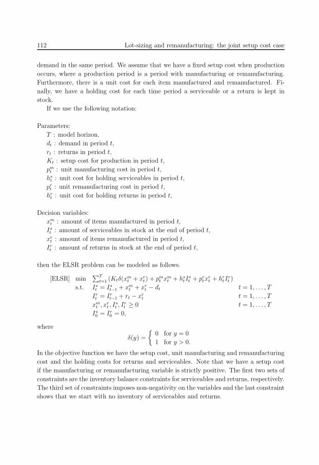
122

112 Lot-sizing and remanufacturing: the joint setup cost case

demand in the same period. We assume that we have a fixed setup cost when production

occurs, where a production period is a period with manufacturing or remanufacturing.

Furthermore, there is a unit cost for each item manufactured and remanufactured. Fi-

nally, we have a holding cost for each time period a serviceable or a return is kept in

stock.

If we use the following notation:

Parameters:

T : model horizon,

dt : demand in period t,

rt : returns in period t,

Kt : setup cost for production in period t,

pmt : unit manufacturing cost in period t,

hst : unit cost for holding serviceables in period t,

prt : unit remanufacturing cost in period t,

hrt : unit cost for holding returns in period t,

Decision variables:

xmt : amount of items manufactured in period t,

Ist : amount of serviceables in stock at the end of period t,

xrt : amount of items remanufactured in period t,

Irt : amount of returns in stock at the end of period t,

then the ELSR problem can be modeled as follows.

[ELSR] min∑T

t=1 (Ktδ(xmt + xr

t ) + pmt xm

t + hstI

st + pr

txrt + hr

tIrt )

s.t. Ist = Is

t−1 + xmt + xr

t − dt t = 1, . . . , T

Irt = Ir

t−1 + rt − xrt t = 1, . . . , T

xmt , xr

t , Ist , I

rt ≥ 0 t = 1, . . . , T

Is0 = Ir

0 = 0,

where

δ(y) =

0 for y = 0

1 for y > 0.

In the objective function we have the setup cost, unit manufacturing and remanufacturing

cost and the holding costs for returns and serviceables. Note that we have a setup cost

if the manufacturing or remanufacturing variable is strictly positive. The first two sets of

constraints are the inventory balance constraints for serviceables and returns, respectively.

The third set of constraints imposes non-negativity on the variables and the last constraint

shows that we start with no inventory of serviceables and returns.

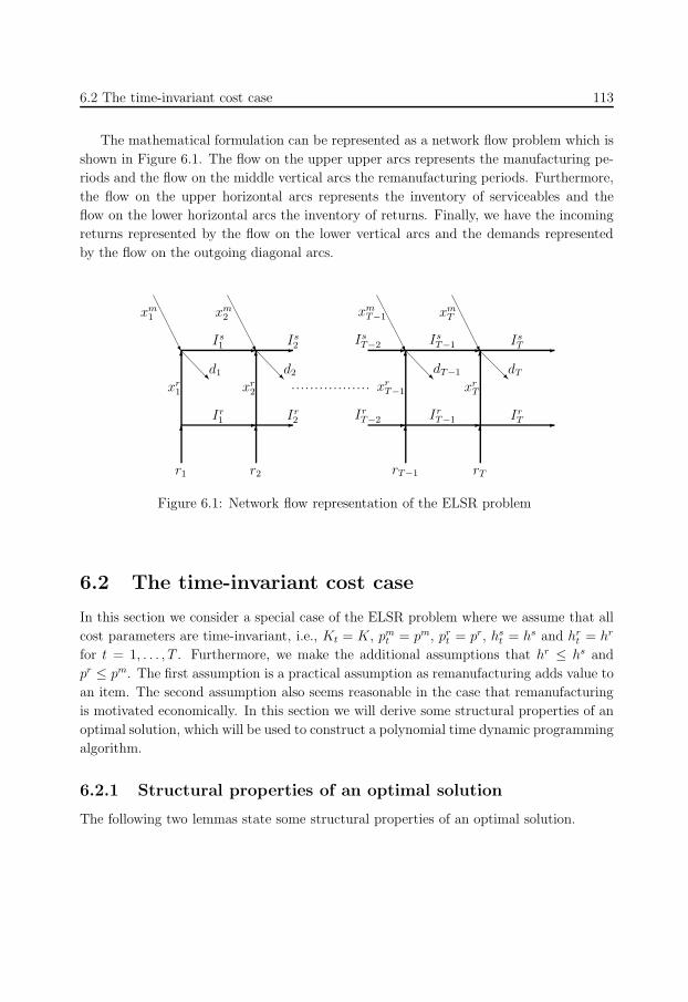
123

6.2 The time-invariant cost case 113

The mathematical formulation can be represented as a network flow problem which is

shown in Figure 6.1. The flow on the upper upper arcs represents the manufacturing pe-

riods and the flow on the middle vertical arcs the remanufacturing periods. Furthermore,

the flow on the upper horizontal arcs represents the inventory of serviceables and the

flow on the lower horizontal arcs the inventory of returns. Finally, we have the incoming

returns represented by the flow on the lower vertical arcs and the demands represented

by the flow on the outgoing diagonal arcs.

6

-

6- Is

2 IsT−2-

6 6

-

- -

-6

- -

R6

-

6

r1

6

r2

R R.................

R

xmTxm

T−1

U U

rT−1 rT

Ir1 Ir

2 IrT−2 Ir

T−1 IrT

xr1 xr

2 xrT−1 xr

T

Is1 Is

T−1 IsT

d1 d2 dT−1 dT

xm1 xm

2

U U

Figure 6.1: Network flow representation of the ELSR problem

6.2 The time-invariant cost case

In this section we consider a special case of the ELSR problem where we assume that all

cost parameters are time-invariant, i.e., Kt = K, pmt = pm, pr

t = pr, hst = hs and hr

t = hr

for t = 1, . . . , T . Furthermore, we make the additional assumptions that hr ≤ hs and

pr ≤ pm. The first assumption is a practical assumption as remanufacturing adds value to

an item. The second assumption also seems reasonable in the case that remanufacturing

is motivated economically. In this section we will derive some structural properties of an

optimal solution, which will be used to construct a polynomial time dynamic programming

algorithm.

6.2.1 Structural properties of an optimal solution

The following two lemmas state some structural properties of an optimal solution.

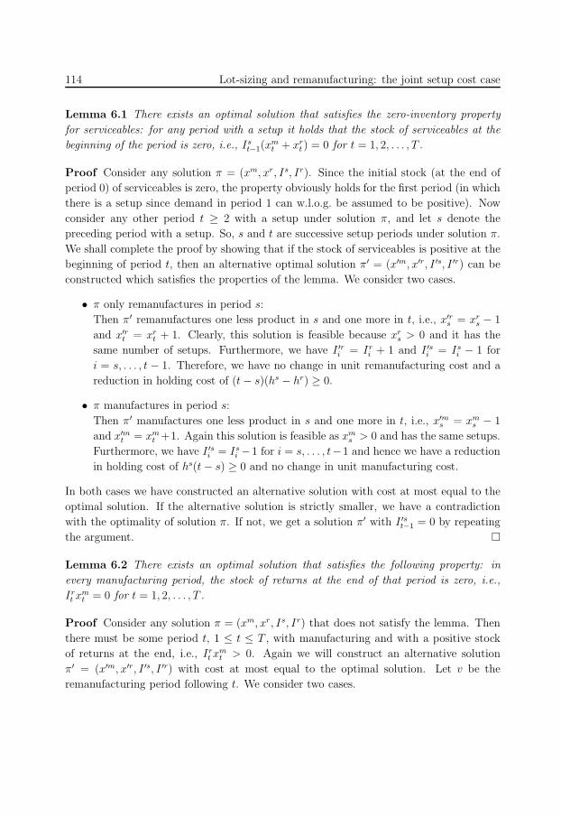
124

114 Lot-sizing and remanufacturing: the joint setup cost case

Lemma 6.1 There exists an optimal solution that satisfies the zero-inventory property

for serviceables: for any period with a setup it holds that the stock of serviceables at the

beginning of the period is zero, i.e., Ist−1(x

mt + xr

t ) = 0 for t = 1, 2, . . . , T .

Proof Consider any solution π = (xm, xr, Is, Ir). Since the initial stock (at the end of

period 0) of serviceables is zero, the property obviously holds for the first period (in which

there is a setup since demand in period 1 can w.l.o.g. be assumed to be positive). Now

consider any other period t ≥ 2 with a setup under solution π, and let s denote the

preceding period with a setup. So, s and t are successive setup periods under solution π.

We shall complete the proof by showing that if the stock of serviceables is positive at the

beginning of period t, then an alternative optimal solution π′ = (x′m, x′r, I ′s, I ′r) can be

constructed which satisfies the properties of the lemma. We consider two cases.

• π only remanufactures in period s:

Then π′ remanufactures one less product in s and one more in t, i.e., x′rs = xr

s − 1

and x′rt = xr

t + 1. Clearly, this solution is feasible because xrs > 0 and it has the

same number of setups. Furthermore, we have I ′ri = Ir

i + 1 and I ′si = Is

i − 1 for

i = s, . . . , t − 1. Therefore, we have no change in unit remanufacturing cost and a

reduction in holding cost of (t − s)(hs − hr) ≥ 0.

• π manufactures in period s:

Then π′ manufactures one less product in s and one more in t, i.e., x′ms = xm

s − 1

and x′mt = xm

t +1. Again this solution is feasible as xms > 0 and has the same setups.

Furthermore, we have I ′si = Is

i −1 for i = s, . . . , t−1 and hence we have a reduction

in holding cost of hs(t − s) ≥ 0 and no change in unit manufacturing cost.

In both cases we have constructed an alternative solution with cost at most equal to the

optimal solution. If the alternative solution is strictly smaller, we have a contradiction

with the optimality of solution π. If not, we get a solution π′ with I ′st−1 = 0 by repeating

the argument.

Lemma 6.2 There exists an optimal solution that satisfies the following property: in

every manufacturing period, the stock of returns at the end of that period is zero, i.e.,

Irt x

mt = 0 for t = 1, 2, . . . , T .

Proof Consider any solution π = (xm, xr, Is, Ir) that does not satisfy the lemma. Then

there must be some period t, 1 ≤ t ≤ T , with manufacturing and with a positive stock

of returns at the end, i.e., Irt x

mt > 0. Again we will construct an alternative solution

π′ = (x′m, x′r, I ′s, I ′r) with cost at most equal to the optimal solution. Let v be the

remanufacturing period following t. We consider two cases.

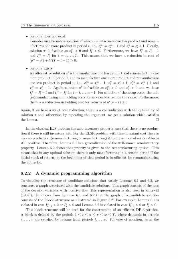
125

6.2 The time-invariant cost case 115

• period v does not exist:

Consider an alternative solution π′ which manufactures one less product and reman-

ufactures one more product in period t, i.e., x′mt = xm

t − 1 and x′rt = xr

t +1. Clearly,

solution π′ is feasible as xmt > 0 and Ir

t > 0. Furthermore, we have I ′ri = Ir

i − 1

and I ′si = Is

i for i = t, . . . , T . This means that we have a reduction in cost of

(pm − pr) + hr(T − t + 1) ≥ 0.

• period v exists:

An alternative solution π′ is to manufacture one less product and remanufacture one

more product in period t, and to manufacture one more product and remanufacture

one less product in period v, i.e., x′mt = xm

t − 1, x′rt = xr

t + 1, x′mv = xm

v + 1 and

x′rv = xr

v − 1. Again, solution π′ is feasible as xmt > 0 and xr

v > 0 and we have

I ′ri = Ir

i −1 and I ′si = Is

i for i = t, . . . , v−1. For solution π′ the setup costs, the unit

(re)manufacturing and holding costs for serviceables remain the same. Furthermore,

there is a reduction in holding cost for returns of hr(v − t) ≥ 0.

Again, if we have a strict cost reduction, there is a contradiction with the optimality of

solution π and, otherwise, by repeating the argument, we get a solution which satisfies

the lemma.

In the classical ELS problem the zero-inventory property says that there is no produc-

tion if there is still inventory left. For the ELSR problem with time-invariant cost there is

also no production (remanufacturing or manufacturing) if the inventory of serviceables is

still positive. Therefore, Lemma 6.1 is a generalization of the well-known zero-inventory

property. Lemma 6.2 shows that priority is given to the remanufacturing option. This

means that in any optimal solution there is only manufacturing in a certain period if the

initial stock of returns at the beginning of that period is insufficient for remanufacturing

the entire lot.

6.2.2 A dynamic programming algorithm

To visualize the structure of candidate solutions that satisfy Lemmas 6.1 and 6.2, we

construct a graph associated with the candidate solutions. This graph consists of the arcs

of the decision variables with positive flow (this representation is also used in Zangwill

(1968)). It follows from Lemmas 6.1 and 6.2 that the graph of a candidate solution

consists of the ‘block’-structure as illustrated in Figure 6.2. For example, Lemma 6.1 is

violated in case Isu−1 > 0 or Is

w > 0 and Lemma 6.2 is violated in case Irt−1 > 0 or Ir

v > 0.

This block-structure will be used for the construction of an efficient DP algorithm.

A block is defined by the periods 1 ≤ t ≤ u ≤ v ≤ w ≤ T , where demands in periods

v, . . . , w are satisfied by returns from periods t, . . . , v. For ease of notation, as in the

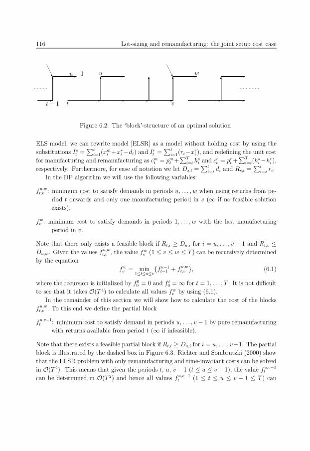
126

116 Lot-sizing and remanufacturing: the joint setup cost case

6U -

-

6-

- -

6

-

6-U

-

6-

-

......... ...............

t

u

v

w

-t − 1

u − 1

Figure 6.2: The ‘block’-structure of an optimal solution

ELS model, we can rewrite model [ELSR] as a model without holding cost by using the

substitutions Ist =

∑ti=1(x

mi +xr

i −di) and Irt =

∑ti=1(ri−xr

i ), and redefining the unit cost

for manufacturing and remanufacturing as cmt = pm

t +∑T

i=t hsi and cr

t = prt +∑T

i=t(hsi −hr

i ),

respectively. Furthermore, for ease of notation we let Ds,t =∑t

i=s di and Rs,t =∑t

i=s ri.

In the DP algorithm we will use the following variables:

fu,wt,v : minimum cost to satisfy demands in periods u, . . . , w when using returns from pe-

riod t onwards and only one manufacturing period in v (∞ if no feasible solution

exists),

fwv : minimum cost to satisfy demands in periods 1, . . . , w with the last manufacturing

period in v.

Note that there only exists a feasible block if Rt,i ≥ Du,i for i = u, . . . , v − 1 and Rt,v ≤Du,w. Given the values fu,w

t,v , the value fwv (1 ≤ v ≤ w ≤ T ) can be recursively determined

by the equation

fwv = min

1≤t≤u≤vfu−1

t−1 + fu,wt,v , (6.1)

where the recursion is initialized by f 00 = 0 and f t

0 = ∞ for t = 1, . . . , T . It is not difficult

to see that it takes O(T 4) to calculate all values fwv by using (6.1).

In the remainder of this section we will show how to calculate the cost of the blocks

fu,wt,v . To this end we define the partial block

fu,v−1t : minimum cost to satisfy demand in periods u, . . . , v − 1 by pure remanufacturing

with returns available from period t (∞ if infeasible).

Note that there exists a feasible partial block if Rt,i ≥ Du,i for i = u, . . . , v−1. The partial

block is illustrated by the dashed box in Figure 6.3. Richter and Sombrutzki (2000) show

that the ELSR problem with only remanufacturing and time-invariant costs can be solved

in O(T 2). This means that given the periods t, u, v − 1 (t ≤ u ≤ v − 1), the value fu,v−1t

can be determined in O(T 2) and hence all values fu,v−1t (1 ≤ t ≤ u ≤ v − 1 ≤ T ) can

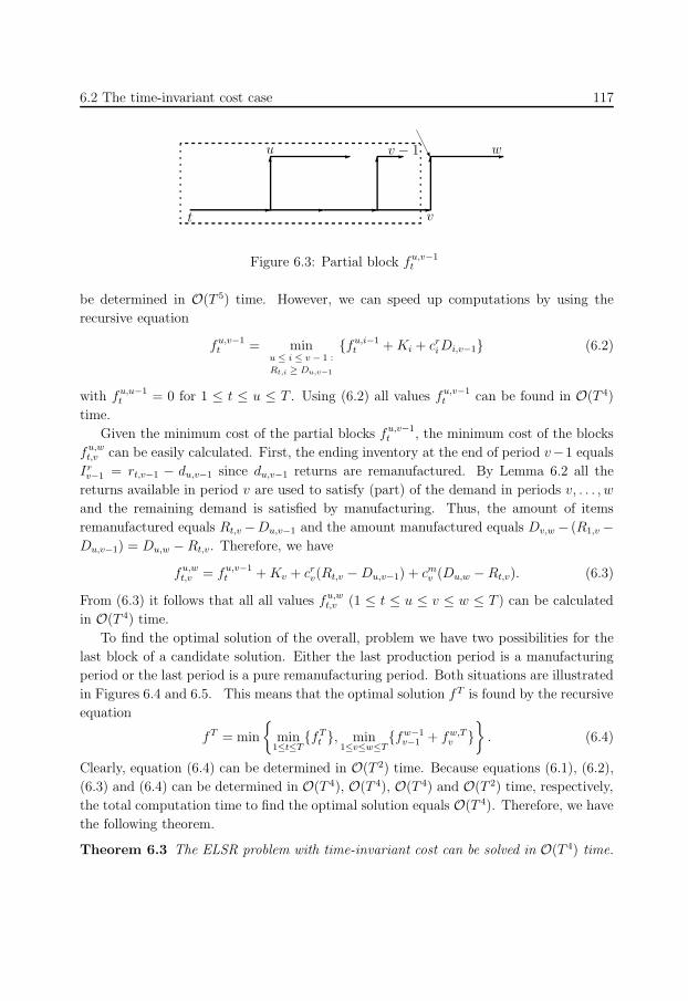
127

6.2 The time-invariant cost case 117

-- v − 1

-

6

- -

6

-

6-U w

t

u

v

Figure 6.3: Partial block fu,v−1t

be determined in O(T 5) time. However, we can speed up computations by using the

recursive equation

fu,v−1t = min

u ≤ i ≤ v − 1 :

Rt,i ≥ Du,v−1

fu,i−1t + Ki + cr

i Di,v−1 (6.2)

with fu,u−1t = 0 for 1 ≤ t ≤ u ≤ T . Using (6.2) all values fu,v−1

t can be found in O(T 4)

time.

Given the minimum cost of the partial blocks fu,v−1t , the minimum cost of the blocks

fu,wt,v can be easily calculated. First, the ending inventory at the end of period v−1 equals

Irv−1 = rt,v−1 − du,v−1 since du,v−1 returns are remanufactured. By Lemma 6.2 all the

returns available in period v are used to satisfy (part) of the demand in periods v, . . . , w

and the remaining demand is satisfied by manufacturing. Thus, the amount of items

remanufactured equals Rt,v −Du,v−1 and the amount manufactured equals Dv,w − (R1,v −Du,v−1) = Du,w − Rt,v. Therefore, we have

fu,wt,v = fu,v−1

t + Kv + crv(Rt,v − Du,v−1) + cm

v (Du,w − Rt,v). (6.3)

From (6.3) it follows that all all values fu,wt,v (1 ≤ t ≤ u ≤ v ≤ w ≤ T ) can be calculated

in O(T 4) time.

To find the optimal solution of the overall, problem we have two possibilities for the

last block of a candidate solution. Either the last production period is a manufacturing

period or the last period is a pure remanufacturing period. Both situations are illustrated

in Figures 6.4 and 6.5. This means that the optimal solution fT is found by the recursive

equation

fT = min

min

1≤t≤TfT

t , min1≤v≤w≤T

fw−1v−1 + fw,T

v

. (6.4)

Clearly, equation (6.4) can be determined in O(T 2) time. Because equations (6.1), (6.2),

(6.3) and (6.4) can be determined in O(T 4), O(T 4), O(T 4) and O(T 2) time, respectively,

the total computation time to find the optimal solution equals O(T 4). Therefore, we have

the following theorem.

Theorem 6.3 The ELSR problem with time-invariant cost can be solved in O(T 4) time.

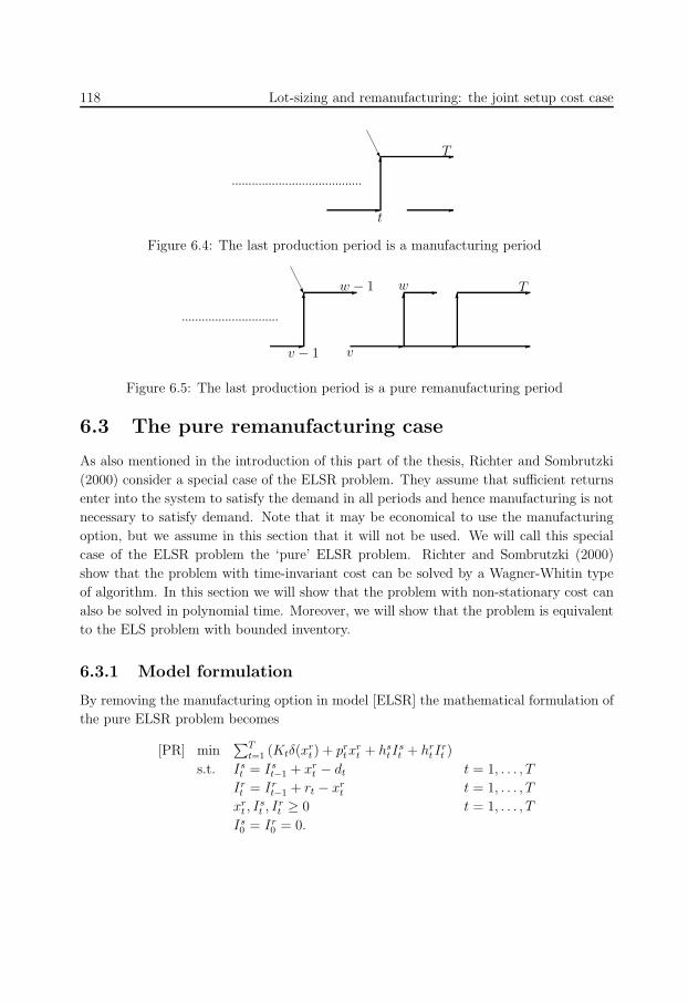
128

118 Lot-sizing and remanufacturing: the joint setup cost case

.......................................

--

6-U T

t

Figure 6.4: The last production period is a manufacturing period

--

6-

6-U

- -

6-

.............................

T

v

ww − 1

v − 1

Figure 6.5: The last production period is a pure remanufacturing period

6.3 The pure remanufacturing case

As also mentioned in the introduction of this part of the thesis, Richter and Sombrutzki

(2000) consider a special case of the ELSR problem. They assume that sufficient returns

enter into the system to satisfy the demand in all periods and hence manufacturing is not

necessary to satisfy demand. Note that it may be economical to use the manufacturing

option, but we assume in this section that it will not be used. We will call this special

case of the ELSR problem the ‘pure’ ELSR problem. Richter and Sombrutzki (2000)

show that the problem with time-invariant cost can be solved by a Wagner-Whitin type

of algorithm. In this section we will show that the problem with non-stationary cost can

also be solved in polynomial time. Moreover, we will show that the problem is equivalent

to the ELS problem with bounded inventory.

6.3.1 Model formulation

By removing the manufacturing option in model [ELSR] the mathematical formulation of

the pure ELSR problem becomes

[PR] min∑T

t=1 (Ktδ(xrt ) + pr

txrt + hs

tIst + hr

t Irt )

s.t. Ist = Is

t−1 + xrt − dt t = 1, . . . , T

Irt = Ir

t−1 + rt − xrt t = 1, . . . , T

xrt , I

st , I

rt ≥ 0 t = 1, . . . , T

Is0 = Ir

0 = 0.

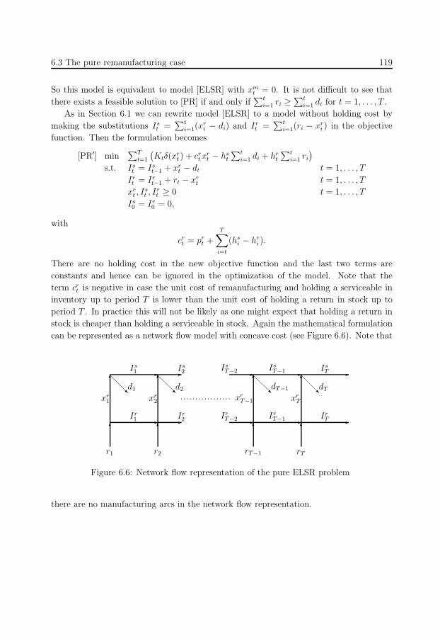
129

6.3 The pure remanufacturing case 119

So this model is equivalent to model [ELSR] with xmt = 0. It is not difficult to see that

there exists a feasible solution to [PR] if and only if∑t

i=1 ri ≥∑t

i=1 di for t = 1, . . . , T .

As in Section 6.1 we can rewrite model [ELSR] to a model without holding cost by

making the substitutions Ist =

∑ti=1(x

ri − di) and Ir

t =∑t

i=1(ri − xri ) in the objective

function. Then the formulation becomes

[PR′] min∑T

t=1

(Ktδ(x

rt ) + cr

txrt − hs

t

∑ti=1 di + hr

t

∑ti=1 ri

)

s.t. Ist = Is

t−1 + xrt − dt t = 1, . . . , T

Irt = Ir

t−1 + rt − xrt t = 1, . . . , T

xrt , I

st , I

rt ≥ 0 t = 1, . . . , T

Is0 = Ir

0 = 0,

with

crt = pr

t +T∑

i=t

(hsi − hr

i ).

There are no holding cost in the new objective function and the last two terms are

constants and hence can be ignored in the optimization of the model. Note that the

term crt is negative in case the unit cost of remanufacturing and holding a serviceable in

inventory up to period T is lower than the unit cost of holding a return in stock up to

period T . In practice this will not be likely as one might expect that holding a return in

stock is cheaper than holding a serviceable in stock. Again the mathematical formulation

can be represented as a network flow model with concave cost (see Figure 6.6). Note that

6

-

6- Is

2 IsT−2-

6 6

-

- -

-6

- -

R6

-

6

r1

6

r2

R R.................

R

rT−1 rT

Ir1 Ir

2 IrT−2 Ir

T−1 IrT

xr1 xr

2 xrT−1 xr

T

Is1 Is

T−1 IsT

d1 d2 dT−1 dT

Figure 6.6: Network flow representation of the pure ELSR problem

there are no manufacturing arcs in the network flow representation.

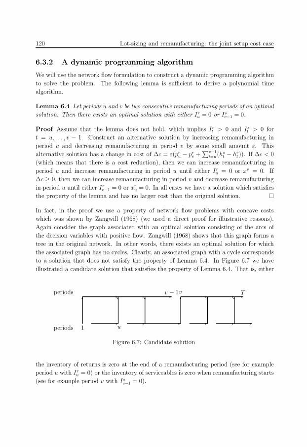
130

120 Lot-sizing and remanufacturing: the joint setup cost case

6.3.2 A dynamic programming algorithm

We will use the network flow formulation to construct a dynamic programming algorithm

to solve the problem. The following lemma is sufficient to derive a polynomial time

algorithm.

Lemma 6.4 Let periods u and v be two consecutive remanufacturing periods of an optimal

solution. Then there exists an optimal solution with either Iru = 0 or Is

v−1 = 0.

Proof Assume that the lemma does not hold, which implies Irt > 0 and Is

t > 0 for

t = u, . . . , v − 1. Construct an alternative solution by increasing remanufacturing in

period u and decreasing remanufacturing in period v by some small amount ε. This

alternative solution has a change in cost of ∆c = ε(pru − pr

v +∑v−1

t=u(hst − hr

t )). If ∆c < 0

(which means that there is a cost reduction), then we can increase remanufacturing in

period u and increase remanufacturing in period u until either Iru = 0 or xv = 0. If

∆c ≥ 0, then we can increase remanufacturing in period v and decrease remanufacturing

in period u until either Irv−1 = 0 or xr

u = 0. In all cases we have a solution which satisfies

the property of the lemma and has no larger cost than the original solution.

In fact, in the proof we use a property of network flow problems with concave costs

which was shown by Zangwill (1968) (we used a direct proof for illustrative reasons).

Again consider the graph associated with an optimal solution consisting of the arcs of

the decision variables with positive flow. Zangwill (1968) shows that this graph forms a

tree in the original network. In other words, there exists an optimal solution for which

the associated graph has no cycles. Clearly, an associated graph with a cycle corresponds

to a solution that does not satisfy the property of Lemma 6.4. In Figure 6.7 we have

illustrated a candidate solution that satisfies the property of Lemma 6.4. That is, either

6-

-

6

-

6-

-

6

-

6-

-

6

1 u

vv − 1 Tperiods

periods

- - -

-

Figure 6.7: Candidate solution

the inventory of returns is zero at the end of a remanufacturing period (see for example

period u with Iru = 0) or the inventory of serviceables is zero when remanufacturing starts

(see for example period v with Isv−1 = 0).

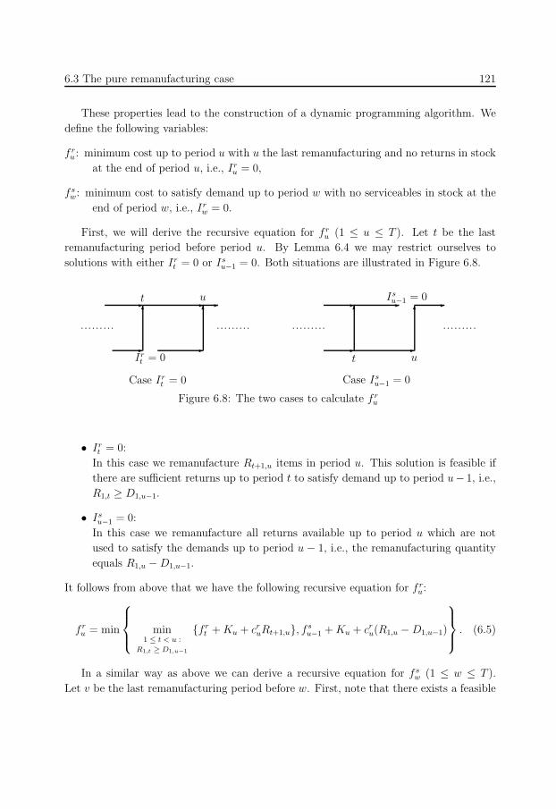
131

6.3 The pure remanufacturing case 121

These properties lead to the construction of a dynamic programming algorithm. We

define the following variables:

f ru : minimum cost up to period u with u the last remanufacturing and no returns in stock

at the end of period u, i.e., Iru = 0,

f sw: minimum cost to satisfy demand up to period w with no serviceables in stock at the

end of period w, i.e., Irw = 0.

First, we will derive the recursive equation for f ru (1 ≤ u ≤ T ). Let t be the last

remanufacturing period before period u. By Lemma 6.4 we may restrict ourselves to

solutions with either Irt = 0 or Is

u−1 = 0. Both situations are illustrated in Figure 6.8.

-

6-

-

6-

......... .........

t u

Irt = 0

Case Irt = 0

.........

-

-

6-

-

6-

.........

t u

Isu−1 = 0

Case Isu−1 = 0

-

Figure 6.8: The two cases to calculate f ru

• Irt = 0:

In this case we remanufacture Rt+1,u items in period u. This solution is feasible if

there are sufficient returns up to period t to satisfy demand up to period u− 1, i.e.,

R1,t ≥ D1,u−1.

• Isu−1 = 0:

In this case we remanufacture all returns available up to period u which are not

used to satisfy the demands up to period u − 1, i.e., the remanufacturing quantity

equals R1,u − D1,u−1.

It follows from above that we have the following recursive equation for f ru:

f ru = min

min

1 ≤ t < u :

R1,t ≥ D1,u−1

f rt + Ku + cr

uRt+1,u, f su−1 + Ku + cr

u(R1,u − D1,u−1)

. (6.5)

In a similar way as above we can derive a recursive equation for f sw (1 ≤ w ≤ T ).

Let v be the last remanufacturing period before w. First, note that there exists a feasible

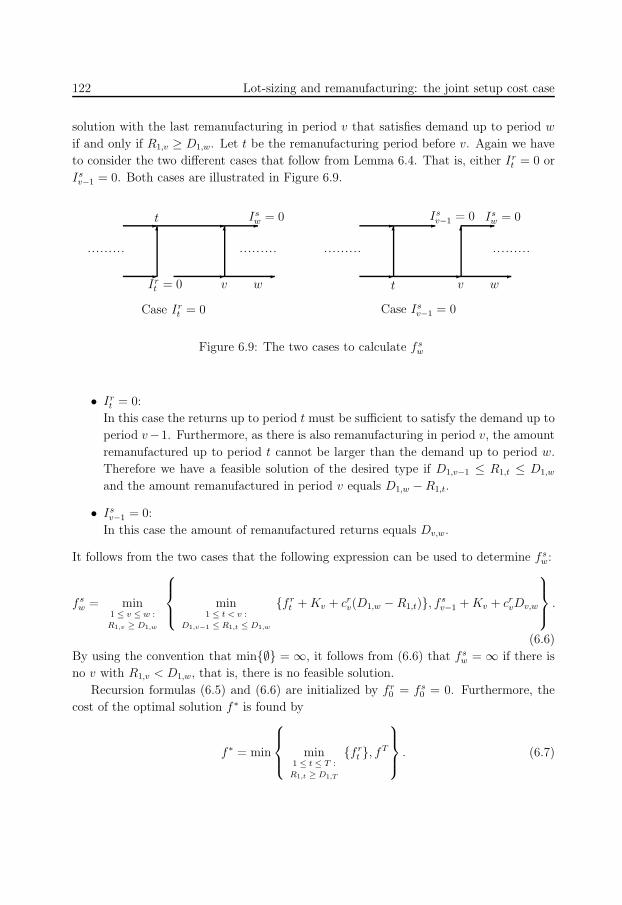
132

122 Lot-sizing and remanufacturing: the joint setup cost case

solution with the last remanufacturing in period v that satisfies demand up to period w

if and only if R1,v ≥ D1,w. Let t be the remanufacturing period before v. Again we have

to consider the two different cases that follow from Lemma 6.4. That is, either Irt = 0 or

Isv−1 = 0. Both cases are illustrated in Figure 6.9.

-

6-

-

6

-

......... .........

t

wIrt = 0

Case Irt = 0

.........

-

-

6-

-

6-

.........

t v

Isv−1 = 0

Case Isv−1 = 0

v-

Isw = 0Is

w = 0

w

- -

Figure 6.9: The two cases to calculate f sw

• Irt = 0:

In this case the returns up to period t must be sufficient to satisfy the demand up to

period v−1. Furthermore, as there is also remanufacturing in period v, the amount

remanufactured up to period t cannot be larger than the demand up to period w.

Therefore we have a feasible solution of the desired type if D1,v−1 ≤ R1,t ≤ D1,w

and the amount remanufactured in period v equals D1,w − R1,t.

• Isv−1 = 0:

In this case the amount of remanufactured returns equals Dv,w.

It follows from the two cases that the following expression can be used to determine f sw:

f sw = min

1 ≤ v ≤ w :

R1,v ≥ D1,w

min

1 ≤ t < v :

D1,v−1 ≤ R1,t ≤ D1,w

f rt + Kv + cr

v(D1,w − R1,t), f sv−1 + Kv + cr

vDv,w

.

(6.6)

By using the convention that min∅ = ∞, it follows from (6.6) that f sw = ∞ if there is

no v with R1,v < D1,w, that is, there is no feasible solution.

Recursion formulas (6.5) and (6.6) are initialized by f r0 = f s

0 = 0. Furthermore, the

cost of the optimal solution f ∗ is found by

f ∗ = min

min

1 ≤ t ≤ T :

R1,t ≥ D1,T

f rt , fT

. (6.7)

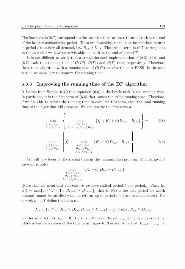
133

6.3 The pure remanufacturing case 123

The first term in (6.7) corresponds to the case that there are no returns in stock at the end

of the last remanufacturing period. To assure feasibility, there must be sufficient returns

in period t to satisfy all demand, i.e., R1,t ≥ D1,T . The second term in (6.7) corresponds

to the case that we have no serviceables in stock at the end of period T .

It is not difficult to verify that a straightforward implementation of (6.5), (6.6) and

(6.7) leads to a running time of O(T 2), O(T 3) and O(T ) time, respectively. Therefore,

there is an algorithm with a running time of O(T 3) to solve the pure ELSR. In the next

section we show how to improve the running time.

6.3.3 Improving the running time of the DP algorithm

It follows from Section 6.3.2 that equation (6.6) is the bottle neck in the running time.

In particular, it is the first term of (6.6) that causes the cubic running time. Therefore,

if we are able to reduce the running time to calculate this term, then the total running

time of the algorithm will decrease. We can rewrite the first term as

min1 ≤ v ≤ w :

R1,v ≥ D1,w

min

1 ≤ t < v :

D1,v−1 ≤ R1,t ≤ D1,w

f rt + Kv + cr

v(D1,w − R1,t)

= (6.8)

min1 ≤ t < w :

R1,t ≤ D1,w

f rt + min

t < v ≤ w :

R1,v ≥ D1,w,

R1,t ≥ D1,v−1

Kv + crv(D1,w − R1,t)

. (6.9)

We will now focus on the second term in this minimization problem. That is, given t

we want to solve

mint ≤ v ≤ w :

R1,v ≥ D1,w,

R1,t−1 ≥ D1,v−1

Kv + crv(D1,w − R1,t−1).

(Note that for notational convenience we have shifted period t one period.) First, let

b(t) = maxw ≤ T + 1 : R1,t−1 ≥ D1,w−1, that is, b(t) is the first period for which

demand cannot be satisfied when all returns up to period t − 1 are remanufactured. For

w = b(t), . . . , T define the index set

Jt,w = v ≤ w : R1,v ≥ D1,w, R1,t−1 ≥ D1,v−1 = v ≤ b(t) : R1,v ≥ D1,w.

and for w < b(t) let Jt,w = ∅. By this definition, the set Jt,w contains all periods for

which a feasible solution of the type as in Figure 6.10 exists. Note that Jt,w+1 ⊆ Jt,w for

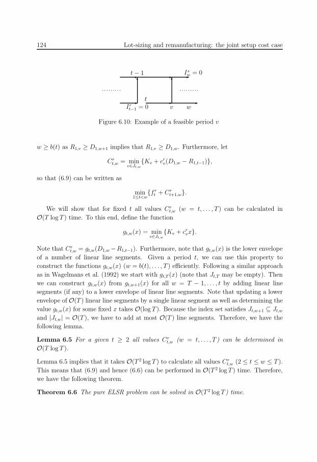
134

124 Lot-sizing and remanufacturing: the joint setup cost case

-

6-

-

6

-

......... .........

t − 1

Irt−1 = 0

tv

Isw = 0

w

- -

Figure 6.10: Example of a feasible period v

w ≥ b(t) as R1,v ≥ D1,w+1 implies that R1,v ≥ D1,w. Furthermore, let

Crt,w = min

v∈Jt,w

Kv + crv(D1,w − R1,t−1),

so that (6.9) can be written as

min1≤t<w

f rt + Cr

t+1,w.

We will show that for fixed t all values Crt,w (w = t, . . . , T ) can be calculated in

O(T log T ) time. To this end, define the function

gt,w(x) = minv∈Jt,w

Kv + crvx.

Note that Crt,w = gt,w(D1,w −R1,t−1). Furthermore, note that gt,w(x) is the lower envelope

of a number of linear line segments. Given a period t, we can use this property to

construct the functions gt,w(x) (w = b(t), . . . , T ) efficiently. Following a similar approach

as in Wagelmans et al. (1992) we start with gt,T (x) (note that Jt,T may be empty). Then

we can construct gt,w(x) from gt,w+1(x) for all w = T − 1, . . . , t by adding linear line

segments (if any) to a lower envelope of linear line segments. Note that updating a lower

envelope of O(T ) linear line segments by a single linear segment as well as determining the

value gt,w(x) for some fixed x takes O(log T ). Because the index set satisfies Jt,w+1 ⊆ Jt,w

and |Jt,w| = O(T ), we have to add at most O(T ) line segments. Therefore, we have the

following lemma.

Lemma 6.5 For a given t ≥ 2 all values Crt,w (w = t, . . . , T ) can be determined in

O(T log T ).

Lemma 6.5 implies that it takes O(T 2 log T ) to calculate all values Crt,w (2 ≤ t ≤ w ≤ T ).

This means that (6.9) and hence (6.6) can be performed in O(T 2 log T ) time. Therefore,

we have the following theorem.

Theorem 6.6 The pure ELSR problem can be solved in O(T 2 log T ) time.

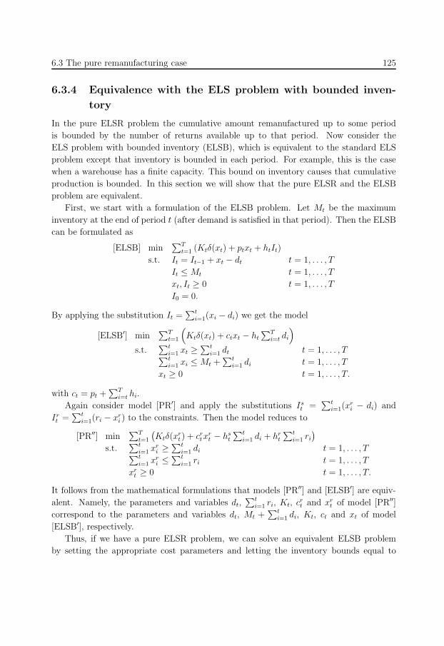
135

6.3 The pure remanufacturing case 125

6.3.4 Equivalence with the ELS problem with bounded inven-

tory

In the pure ELSR problem the cumulative amount remanufactured up to some period

is bounded by the number of returns available up to that period. Now consider the

ELS problem with bounded inventory (ELSB), which is equivalent to the standard ELS

problem except that inventory is bounded in each period. For example, this is the case

when a warehouse has a finite capacity. This bound on inventory causes that cumulative

production is bounded. In this section we will show that the pure ELSR and the ELSB

problem are equivalent.

First, we start with a formulation of the ELSB problem. Let Mt be the maximum

inventory at the end of period t (after demand is satisfied in that period). Then the ELSB

can be formulated as

[ELSB] min∑T

t=1 (Ktδ(xt) + ptxt + htIt)

s.t. It = It−1 + xt − dt t = 1, . . . , T

It ≤ Mt t = 1, . . . , T

xt, It ≥ 0 t = 1, . . . , T

I0 = 0.

By applying the substitution It =∑t

i=1(xi − di) we get the model

[ELSB′] min∑T

t=1

(Ktδ(xt) + ctxt − ht

∑Ti=t di

)

s.t.∑t

i=1 xt ≥∑t

i=1 dt t = 1, . . . , T∑ti=1 xi ≤ Mt +

∑ti=1 di t = 1, . . . , T

xt ≥ 0 t = 1, . . . , T.

with ct = pt +∑T

i=t hi.

Again consider model [PR′] and apply the substitutions Ist =

∑ti=1(x

ri − di) and

Irt =

∑ti=1(ri − xr

i ) to the constraints. Then the model reduces to

[PR′′] min∑T

t=1

(Ktδ(x

rt ) + cr

txrt − hs

t

∑ti=1 di + hr

t

∑ti=1 ri

)

s.t.∑t

i=1 xri ≥

∑ti=1 di t = 1, . . . , T∑t

i=1 xri ≤

∑ti=1 ri t = 1, . . . , T

xrt ≥ 0 t = 1, . . . , T.

It follows from the mathematical formulations that models [PR′′] and [ELSB′] are equiv-

alent. Namely, the parameters and variables dt,∑t

i=1 ri, Kt, crt and xr

t of model [PR′′]

correspond to the parameters and variables dt, Mt +∑t

i=1 di, Kt, ct and xt of model

[ELSB′], respectively.

Thus, if we have a pure ELSR problem, we can solve an equivalent ELSB problem

by setting the appropriate cost parameters and letting the inventory bounds equal to

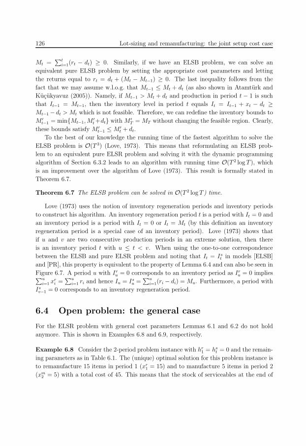
136

126 Lot-sizing and remanufacturing: the joint setup cost case

Mt =∑t

i=1(rt − dt) ≥ 0. Similarly, if we have an ELSB problem, we can solve an

equivalent pure ELSB problem by setting the appropriate cost parameters and letting

the returns equal to rt = dt + (Mt − Mt−1) ≥ 0. The last inequality follows from the

fact that we may assume w.l.o.g. that Mt−1 ≤ Mt + dt (as also shown in Atamturk and

Kucukyavuz (2005)). Namely, if Mt−1 > Mt + dt and production in period t − 1 is such

that It−1 = Mt−1, then the inventory level in period t equals It = It−1 + xt − dt ≥Mt−1 − dt > Mt which is not feasible. Therefore, we can redefine the inventory bounds to

M ′t−1 = minMt−1, M

′t +dt with M ′

T = MT without changing the feasible region. Clearly,

these bounds satisfy M ′t−1 ≤ M ′

t + dt.

To the best of our knowledge the running time of the fastest algorithm to solve the

ELSB problem is O(T 3) (Love, 1973). This means that reformulating an ELSB prob-

lem to an equivalent pure ELSR problem and solving it with the dynamic programming

algorithm of Section 6.3.2 leads to an algorithm with running time O(T 2 log T ), which

is an improvement over the algorithm of Love (1973). This result is formally stated in

Theorem 6.7.

Theorem 6.7 The ELSB problem can be solved in O(T 2 log T ) time.

Love (1973) uses the notion of inventory regeneration periods and inventory periods

to construct his algorithm. An inventory regeneration period t is a period with It = 0 and

an inventory period is a period with It = 0 or It = Mt (by this definition an inventory

regeneration period is a special case of an inventory period). Love (1973) shows that

if u and v are two consecutive production periods in an extreme solution, then there

is an inventory period t with u ≤ t < v. When using the one-to-one correspondence

between the ELSB and pure ELSR problem and noting that It = Ist in models [ELSB]

and [PR], this property is equivalent to the property of Lemma 6.4 and can also be seen in

Figure 6.7. A period u with Iru = 0 corresponds to an inventory period as Ir

u = 0 implies∑ui=1 xr

i =∑u

i=1 ri and hence Iu = Isu =

∑ui=1(ri − di) = Mu. Furthermore, a period with

Isv−1 = 0 corresponds to an inventory regeneration period.

6.4 Open problem: the general case

For the ELSR problem with general cost parameters Lemmas 6.1 and 6.2 do not hold

anymore. This is shown in Examples 6.8 and 6.9, respectively.

Example 6.8 Consider the 2-period problem instance with hr1 = hs

t = 0 and the remain-

ing parameters as in Table 6.1. The (unique) optimal solution for this problem instance is

to remanufacture 15 items in period 1 (xr1 = 15) and to manufacture 5 items in period 2

(xm2 = 5) with a total cost of 45. This means that the stock of serviceables at the end of

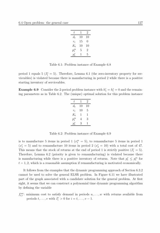
137

6.4 Open problem: the general case 127

t 1 2

dt 10 10

rt 15 0

Kt 10 10

pmt 5 2

prt 1 5

Table 6.1: Problem instance of Example 6.8

period 1 equals 5 (Is1 = 5). Therefore, Lemma 6.1 (the zero-inventory property for ser-

viceables) is violated because there is manufacturing in period 2 while there is a positive

starting inventory of serviceables.

Example 6.9 Consider the 2-period problem instance with hr1 = hs

t = 0 and the remain-

ing parameters as in Table 6.2. The (unique) optimal solution for this problem instance

t 1 2

dt 10 10

rt 10 5

Kt 1 1

pmt 4 3

prt 3 1

Table 6.2: Problem instance of Example 6.9

is to manufacture 5 items in period 1 (xm1 = 5), to remanufacture 5 items in period 1

(xr1 = 5) and to remanufacture 10 items in period 2 (xr

2 = 10) with a total cost of 47.

This means that the stock of returns at the end of period 1 is strictly positive (Ir1 = 5).

Therefore, Lemma 6.2 (priority is given to remanufacturing) is violated because there

is manufacturing while there is a positive inventory of returns. Note that prt ≤ pm

t for

t = 1, 2, which is a reasonable assumption if remanufacturing is motivated economically.

It follows from the examples that the dynamic programming approach of Section 6.3.2

cannot be used to solve the general ELSR problem. In Figure 6.11 we have illustrated

part of the graph associated with a candidate solution for the general problem. At first

sight, it seems that we can construct a polynomial time dynamic programming algorithm

by defining the variable

fuwt,v : minimum cost to satisfy demand in periods u, . . . , w with returns available from

periods t, . . . , v with Iri > 0 for i = t, . . . , v − 1.

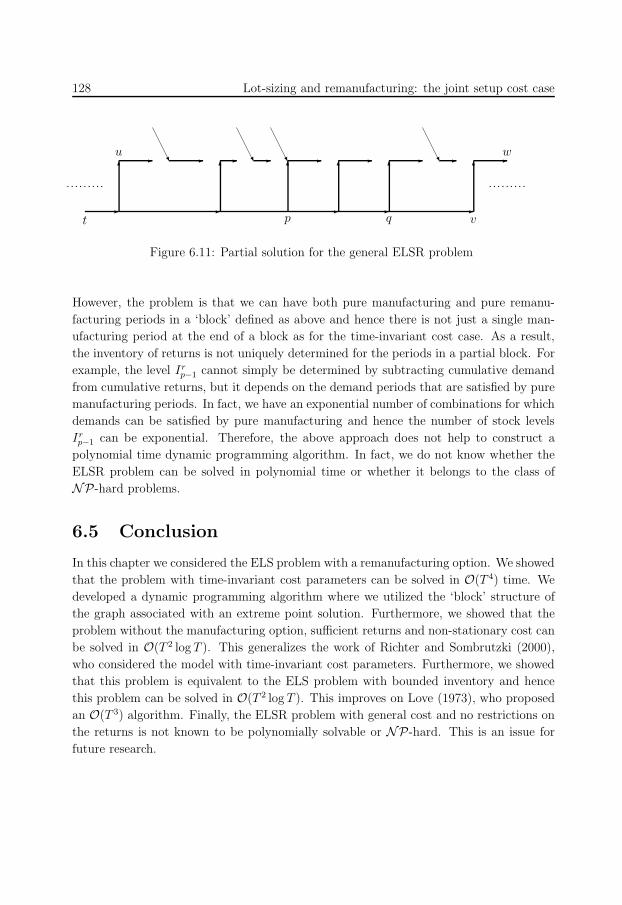
138

128 Lot-sizing and remanufacturing: the joint setup cost case

-

6- U -

-

6-

-

U-6

- - U

-

6- -U

-

6-

......... .........

u

vt

w

p q

6

Figure 6.11: Partial solution for the general ELSR problem

However, the problem is that we can have both pure manufacturing and pure remanu-

facturing periods in a ‘block’ defined as above and hence there is not just a single man-

ufacturing period at the end of a block as for the time-invariant cost case. As a result,

the inventory of returns is not uniquely determined for the periods in a partial block. For

example, the level Irp−1 cannot simply be determined by subtracting cumulative demand

from cumulative returns, but it depends on the demand periods that are satisfied by pure

manufacturing periods. In fact, we have an exponential number of combinations for which

demands can be satisfied by pure manufacturing and hence the number of stock levels

Irp−1 can be exponential. Therefore, the above approach does not help to construct a

polynomial time dynamic programming algorithm. In fact, we do not know whether the

ELSR problem can be solved in polynomial time or whether it belongs to the class of

NP-hard problems.

6.5 Conclusion

In this chapter we considered the ELS problem with a remanufacturing option. We showed

that the problem with time-invariant cost parameters can be solved in O(T 4) time. We

developed a dynamic programming algorithm where we utilized the ‘block’ structure of

the graph associated with an extreme point solution. Furthermore, we showed that the

problem without the manufacturing option, sufficient returns and non-stationary cost can

be solved in O(T 2 log T ). This generalizes the work of Richter and Sombrutzki (2000),

who considered the model with time-invariant cost parameters. Furthermore, we showed

that this problem is equivalent to the ELS problem with bounded inventory and hence

this problem can be solved in O(T 2 log T ). This improves on Love (1973), who proposed

an O(T 3) algorithm. Finally, the ELSR problem with general cost and no restrictions on

the returns is not known to be polynomially solvable or NP-hard. This is an issue for

future research.

139

Chapter 7

The economic lot-sizing problem

with a remanufacturing option and

separate setup cost∗

Abstract

In this chapter we consider the economic lot-sizing problem with a remanufacturing

option. We assume that products come back from the customers and those returned

products can be remanufactured to satisfy demand. In this chapter we assume that

there is separate setup cost when remanufacturing or manufacturing occurs. For

instance, this can be the case when both manufacturing and remanufacturing are

performed on different production lines. We will show that this problem is NP-

hard even in the case of time-invariant cost. Furthermore, we will develop a genetic

algorithm for the problem.

7.1 Problem description and mathematical model

The economic lot-sizing problem with a remanufacturing option and separate setup cost

(ELSR) is equivalent to the problem of Section 6.1 except that there is a setup cost

for both manufacturing and remanufacturing. For example, this is the case when the

manufacturing process and remanufacturing process are performed on different production

lines. In this chapter we will again use the abbreviation ELSR as we also did for the joint

setup cost case in the previous chapter. However, no ambiguity will occur as we will only

consider the separate setup cost case in this chapter. Using the additional notation

Kmt : setup cost for manufacturing in period t,

∗This chapter is based on Van den Heuvel (2004) and Teunter, Bayındır and Van den Heuvel (2006).

140

130 Lot-sizing and remanufacturing: the separate setup cost case

Krt : setup cost for remanufacturing in period t,

the ELSR problem can be modeled as follows:

[ELSR] min∑T

t=1 (Kmt δ(xm

t ) + pmt xm

t + hstI

st + Kr

t δ(xrt ) + pr

txrt + hr

t Irt )

s.t. Ist = Is

t−1 + xmt + xr

t − dt t = 1, . . . , T

Irt = Ir

t−1 + rt − xrt t = 1, . . . , T

xmt , xr

t , Ist , I

rt ≥ 0 t = 1, . . . , T

Is0 = Ir

0 = 0,

where

δ(y) =

0 for y = 0

1 for y > 0.

Note that the mathematical model is equivalent to the mathematical model of Section 6.1

except that the term Kmt δ(xm

t ) + Krt δ(x

rt ) occurs in the objective function in stead of the

term Ktδ(xmt + xr

t ).

In the remainder of this chapter we will analyze this problem. In Section 7.2 we

will show that the problem is NP-hard and we will derive complexity results for related

problems. In the next section we will derive structural properties of an optimal solution.

In Section 7.4 we will consider the ELSR problem where the production periods are fixed

and the optimal production quantities have to be determined. This problem will be the

basis for the genetic algorithm developed in Section 7.5. The chapter is ended with the

conclusion in Section 7.6.

7.2 Complexity results

7.2.1 The general ELSR problem

As mentioned in the introduction Richter and Sombrutzki (2000) and Richter and Weber

(2001) show that some special cases of the ELSR problem can be solved in polynomial

time. However, Richter and Sombrutzki (2000, p. 311) mention that “There are probably

no simple algorithms to solve that general model . . . ”. In this section we will show that

the ELSR problem is NP-hard in general. In the proof we will use a reduction from

the well-known NP-complete PARTITION problem. For complexity theory we refer to

Garey and Johnson (1979) and Papadimitriou and Steiglitz (1982).

Problem PARTITION (problem [SP12] in Garey and Johnson (1979)): Given n positive

integer a1, . . . , an. Does there exist a set S ⊂ N = 1, . . . , n such that∑

i∈S ai =∑i∈N\S ai = A? (Note that we may assume without loss of generality that ai < A for

i = 1, . . . , n.)

141

7.2 Complexity results 131

Theorem 7.1 The ELSR problem with separate setup cost is NP-hard for time-invariant

cost parameters.

Proof Given an instance of PARTITION, define an instance for the ELSR problem as

follows:

T = n,

dt = at for t = 1, . . . , T ,

r1 = A, rt = 0 for t = 2, . . . , T ,

Kmt = Kr

t = 1 for t = 1, . . . , T ,

pmt = 1 for t = 1, . . . , T ,

prt = 0 for t = 1, . . . , T ,

hst = 3 for t = 1, . . . , T ,

hrt = 0 for t = 1, . . . , T .

Clearly, this reduction can be done in polynomial time. We will show that the answer to

PARTITION is positive if and only if the ELSR instance has a solution with cost at most

T + A.

• if part:

Assume that we have a solution for the ELSR instance with cost at most T +

A. First, if serviceables are held in stock, then a solution with strictly less cost

can be constructed. Assume that such a period exists. Then there must be a

(re)manufacturing period t with at least one item in stock at the end of period t.

Decreasing the number of items being (re)manufactured by one in period t and

increasing the number of items being (re)manufactured by one in period t + 1 will

reduce the total cost by at least 1. By repeating the above procedure we get a

solution without serviceables in stock and hence we may restrict ourselves to a

solution with cost at most T + A where no serviceables are held in stock.

Furthermore, because at most A items can be remanufactured and all demand has

to be satisfied, we incur at least variable cost A for manufactured items and we incur

exactly cost A if all returns are remanufactured. Finally, if there is both remanu-

facturing and manufacturing in at least one period, then the total setup costs will

exceed T . Because the total cost is at most T +A, demand in each period is satisfied

by either manufacturing or remanufacturing and the total amount remanufactured

equals A. Therefore, the remanufacturing periods (or the manufacturing periods)

form the set S.

• only if part:

Let S be the set for which∑

i∈S ai =∑

i∈N\S ai = A. It is easy to verify that by

remanufacturing at items in each period t ∈ S and manufacturing at items in each

period t ∈ N\S all demand is satisfied and total costs equal T + A.

142

132 Lot-sizing and remanufacturing: the separate setup cost case

Note that the ELSR problem instance in the proof has reasonable assumptions on

the cost parameters. As already mentioned in Chapter 6, remanufacturing adds value

to an item and hence it is reasonable to assume that holding serviceables is at least as

costly as holding returns (i.e., hst ≥ hr

t ). Furthermore, if remanufacturing is motivated

economically, then the assumption that the unit remanufacturing cost equals at most the

unit manufacturing cost (i.e., pmt ≥ pr

t ) is also reasonable. Finally, in practice it is likely

that the total amount of demand will be larger than the total amount of returns (i.e.,∑Tt=1 dt ≥

∑Tt=1 rt).

Note that the solution for the PARTITION instance and the optimal cost of the ELSR

instance are independent of the ordering of a1, . . . , an (as in the NP-completeness proof

for the capacitated lot-sizing problem (Florian et al., 1980)). This shows that the ELSR

problem is also NP-hard in the case of increasing (or decreasing) demand over time and

time-invariant cost parameters.

In the literature there are some models related to the ELSR model. In the following

two sections we will derive alternative proofs, stronger results and new results for those

related models.

7.2.2 The ELSR problem with a disposal option

Golany et al. (2001) and Yang et al. (2005) consider the ELSR problem with an additional

disposal option (ELSRD for short). If we introduce the additional notation

xdt : the number of items disposed of in period t,

Kdt : setup cost for disposing items in period t,

pdt : unit cost for disposing an item in period t,

then the ELSRD problem can be formulated as

[ELSRD] min∑T

t=1(Kmt δ(xm

t ) + pmt xm

t + hstI

st K

rt δ(x

rt ) + pr

txrt + hr

tIrt

+Kdt δ(xd

t ) + pdt x

dt )

s.t. Ist = Is

t−1 + xmt + xr

t − dt t = 1, . . . , T

Irt = Ir

t−1 + rt − xrt − xd

t t = 1, . . . , T

xmt , xr

t , xdt , I

st , I

rt ≥ 0 t = 1, . . . , T

Is0 = Ir

0 = 0,

where

δ(y) =

0 for y = 0

1 for y > 0.

143

7.2 Complexity results 133

Model [ELSRD] is equivalent to model [ELSR] except that there is an additional term

Kdt δ(xd

t ) + pdt x

dt in the objective function and a term xd

t in the return inventory balance

constraints, which shows that the inventory of returns will decrease if items are disposed

of. Golany et al. (2001) and Yang et al. (2005) present a more general model where

all cost functions are assumed to be general concave functions instead of (setup-)linear

functions. However, for the complexity proofs it is sufficient to consider the formulation

with (setup-)linear costs as a (setup-)linear function is a special case of a concave function.

Golany et al. (2001) show that the ELSRD problem is NP-hard for non-stationary cost

parameters and Yang et al. (2005) improve this result by showing that it is also NP-hard

for the time-invariant cost case.

Yang et al. (2005) argue that there are some similarities between the ELSRD problem

and the capacitated lot-sizing (CLS) problem. In this section we will show that every

CLS problem is equivalent to a special case of the ELSRD without manufacturing. As

the CLS problem is NP-hard (Florian et al., 1980), this immediately implies that the

ELSRD problem is NP-hard.

The CLS problem is equivalent to the ELS problem except that there is a production

capacity in each period. If we let

Ct: the production capacity in period t,

and we use the same notation as for the ELS problem, then the CLS problem can be

formulated as

[CLS] min∑T

t=1 (Ktδ(xt) + ptxt + htIt)

s.t. It = It−1 + xt − dt t = 1, . . . , T

xt + ut = Ct t = 1, . . . , T

xt, ut, It ≥ 0 t = 1, . . . , T

I0 = 0,

where ut is the quantity of unused capacity in period t.

Consider the special case of the ELSRD problem with sufficient returns to satisfy

demand, no manufacturing, no option to hold returns in stock and no disposal cost.

The latter is forced when we impose the conditions R1,t ≥ D1,t, Kmt = hr

t = ∞ and

Kdt = pd

t = 0 for t = 1, . . . , T on model [ELSRD]. In an optimal solution for this special

case no manufacturing will occur (xmt = 0) and no returns will be held in stock (Ir

t = 0).

Hence, the model can be rewritten to

[ELSRD′] min∑T

t=1 (Krt δ(x

rt ) + pr

txrt + hs

tIst )

s.t. Ist = Is

t−1 + xrt − dt t = 1, . . . , T

xrt + xd

t = rt t = 1, . . . , T

xrt , x

dt , I

st ≥ 0 t = 1, . . . , T

Is0 = 0.

144

134 Lot-sizing and remanufacturing: the separate setup cost case

It follows immediately from the mathematical formulation that models [CLS] and [ELSRD′]

are equivalent. That is, producing, holding items and not using capacity in [CLS] corre-

spond to remanufacturing, holding serviceables and disposing in [ELSRD′], respectively.

Therefore, we have the following theorem.

Theorem 7.2 The ELSRD problem is a generalization of the CLS problem.

Bitran and Yanasse (1982) show that the CLS problem with time-invariant cost pa-

rameters (among other families of problem instances) is NP-hard. This implies that the

ELSRD problem with time-invariant cost is NP-hard. This means that we have an alter-

native proof for the complexity result in Yang et al. (2005). Because the ELSRD problem

is a generalization of the ELSR problem and the ELSR problem with time-invariant cost is

NP-hard, the result is also immediately obtained from Theorem 7.1. Thus, the following

corollary follows both from Theorem 7.1 and Theorem 7.2.

Corollary 7.3 The ELSRD problem with time-invariant cost is NP-hard.

7.2.3 The ELSRD problem with fixed ending inventories

Yang et al. (2005) actually consider a model which is slightly different from model

[ELSDR]. They assume that the ending inventories of returns and serviceables (IrT and Is

T )

are not decision variables but fixed parameters. They show that every T -period ELSRD

problem with variable ending inventories can be converted into a (T + 1)-period ELSRD

problem with fixed ending inventories equal to zero. This is done by constructing an

artificial period T + 1 with demand dT+1 = R1,T (note that there will never be more than

R1,T serviceables in stock if the costs are positive), returns rT+1 = 0, zero manufacturing

and disposal cost (KmT+1 = pm

T+1 = KdT+1 = pd

T+1 = 0) and infinitely large remanufacturing

cost (KrT+1 = pr

T+1 = ∞). For this modified instance, returns left in stock in period T

can be disposed of at zero cost in period T + 1 and demand not satisfied by serviceables

in stock at the end of period T can be manufactured at zero cost in period T + 1. This

means that there exists an optimal solution with zero cost in period T + 1 and zero stock

left in period T + 1. Moreover, this solution also gives an optimal solution for the T -

period problem with variable ending inventories. Therefore, Yang et al. (2005) restrict

themselves to the problem with fixed ending inventories.

We can perform a similar ‘trick’ to the ELSR problem (without disposals). We add

an additional period T + 1 with the same parameters as above except that we set the

remanufacturing cost to zero, i.e., KrT+1 = pr

T+1 = 0. Again, solving the (T + 1)-period

problem with the restriction IrT+1 = Is

T+1 = 0 gives an optimal solution for the T -period

problem with variable ending inventories. In the remainder of this section we will consider

the complexity of the ELSR problem with zero ending inventories (denoted by ELSR0).

145

7.2 Complexity results 135

We will show that we can derive stronger complexity results for the ELSR0 problem than

for the ELSR problem. Note that if the T -period problem has time-invariant cost, then

this property does not necessarily hold anymore for the converted (T +1)-period instance.

Therefore, complexity results derived for the ELSR problem with time-invariant cost do

not necessarily hold for the ELSR0 problem with time-invariant cost. The following

theorem shows that the ELSR0 problem is NP-hard.

Theorem 7.4 The ELSR0 problem with time-invariant cost and zero unit manufacturing,

remanufacturing and holding cost for returns is NP-hard.

Proof We will use a reduction from problem PARTITION. Define a problem instance

for the ELSR0 problem as follows:

T = n,

dt = at for t = 1, . . . , T ,

r1 = A, rt = 0 for t = 2, . . . , T ,

Km = Kr = 1,

hs = 2,

pm = pr = hr = 0.

We will show that the answer to PARTITION is yes if and only if the ELSR0 problem has

a solution with cost at most T . First, the cost to satisfy demand dt is at least 1, because

this demand is satisfied by manufacturing, remanufacturing or serviceables in stock. More

precisely, we have a solution with cost at most T if in each period demand is satisfied

by either pure manufacturing or pure remanufacturing (and not by serviceables in stock).

Because the stock of returns must be zero at the end of period T , there exists a solution

with cost at most T if and only there exists a subset of demand periods for which the

sum of demands equals the returns in period 1, i.e., there exists an S ⊂ N = 1, . . . , nsuch that

∑i∈S ai = A.

The problem instance in the proof has a trivial optimal solution with cost T for the

ELSR problem with variable ending inventories. Namely, manufacturing an amount of

dt in each period t = 1, . . . , T is a solution with a manufacturing setup cost of 1 in each

period and hence total cost T . In the following theorem we derive a stronger result for

the ELSR0 problem.

Theorem 7.5 Unless P = NP, there does not exist a polynomial time ε-approximation

algorithm with ε < 1T

for the ELSR0 problem.

Proof Again consider the problem instance of the proof of Theorem 7.4. First, we

construct a simple polynomial time heuristic for such instances. Let p be the (unique)

period that satisfies∑p−1

i=1 ai < A ≤ ∑pi=1 ai. Then xr

t = at (t = 1, . . . , p − 1), xrp =

146

136 Lot-sizing and remanufacturing: the separate setup cost case

A−∑p−1i=1 ai, xm

p = ap − xrp and xm

t = at (t = p + 1, . . . , T ) is a feasible solution with cost

at most T + 1 (the cost equals T if∑p

i=1 ai = A). So the cost of the heuristic solution

CH satisfies CH ≤ T +1. Furthermore, from the the proof of Theorem 7.4 and the simple

heuristic it follows that the cost of the optimal solution C∗ satisfies C∗ ∈ T, T +1. This

means thatCH − C∗

C∗≤ 1

T

and hence the simple heuristic is an 1T-approximation algorithm for this class of problem

instances.

Now assume that we have a polynomial time ε-approximation algorithm with ε < 1T

and denote the cost of a solution by CA. Consider the following cases:

• C∗ = T :

The solution found by the ε-approximation algorithm satisfies

CA ≤ (1 + ε)C∗ = (1 + ε)T < (1 +1

T)T = T + 1.

Because the cost must be integral, this implies that CA = T = C∗ and hence we

have found the optimal solution in polynomial time.

• C∗ = T + 1:

In this case the ε-approximation algorithm finds a solution with CA ≥ T + 1 and

hence we know that C∗ > T implying C∗ = T + 1. Now the optimal solution can

be found in polynomial time by applying the simple heuristic.

From both cases it follows that given a polynomial time ε-approximation algorithm with

ε < 1T

we can solve the ELSR0 instance in polynomial time. But then problem PARTI-

TION can also be solved in polynomial time, which would imply that P = NP.

The following corollary follows from Theorem 7.5.

Corollary 7.6 Unless P = NP, there does not exist a fully polynomial time approxima-

tion scheme (FPTAS) for the ELSR0 problem.

Proof Assume there exists a FPTAS that runs in O(p(|I|) 1εn ) time, where p(x) is a

polynomial, |I| the size of the problem instance and n some fixed integer. Consider the

problem instance in the proof of Theorem 7.4 and let ε = 12T

. It follows from the proof of

Theorem 7.5 that for ε = 12T

the problem instance is solved to optimality. But then the

problem instance is solved in O(p(|I|)T n) which would imply that problem PARTITION

can be solved in polynomial time. This is a contradiction, unless P = NP.

Because the ELSR0 problem is a special case of the ELRSD problem with fixed ending

inventories, Theorem 7.5 and Corollary 7.6 also hold for this problem. These results are

stronger than the results in Yang et al. (2005).

147

7.3 Properties of an optimal solution 137

7.3 Properties of an optimal solution

Although the ELSR problem is NP-hard, we can find some properties of an optimal

solution. To describe these properties we will need some definitions. As in Chapter 6

we will use the notion of regeneration periods. As we have two types of inventory, we

also have two types of regeneration periods. We call period t a serviceable regeneration

period if Ist = 0 and (u, v) is called a serviceable regeneration interval if Is

u−1 = Isv = 0

and Ist > 0 for t ∈ [u, v − 1] (we use [s, t] as a shorthand notation for the set s, . . . , t).

Similarly, period t is called a return regeneration period if Irt = 0 and (u, v) is called a

return regeneration interval if Iru−1 = Ir

v = 0, Ist > 0 and xr

v > 0 for t ∈ [u, v − 1] (we

add the condition xrv > 0 to exclude a series of zero return periods to be a regeneration

interval).

Furthermore, let u and v (u ≤ v) be consecutive production periods with u a reman-

ufacturing period and v a manufacturing period (or opposite). We call (u, v) a connected

pair if Ist > 0 for t ∈ [u, v − 1]. In case u is a manufacturing period and v a remanufac-

turing period, we will call (u, v) a MR connected pair and in case u is a remanufacturing

period and v a manufacturing period, we will call (u, v) a RM connected pair. From the

definition above it follows that if t is both a manufacturing and remanufacturing period,

then (t, t) is also a connected pair. We will call this special case a connected period.

If we use the network formulation of Section 6.1 and the results of Zangwill (1968),

then the following lemmas can be derived.

Lemma 7.7 Let (s, t) be a serviceable regeneration interval in an optimal solution. Then

there exists an optimal solution with at most one manufacturing period between periods s

and t.

Lemma 7.8 Let (s, t) be a return regeneration interval in an optimal solution. Then

there exists an optimal solution with at most one connected pair between periods s and t.

Lemma 7.9 Let s be the last remanufacturing period that satisfies Irs = 0 (s = 0 if this

period does not exist) and let t be the first remanufacturing period after s (if any). Then

there exists an optimal solution for which periods [t, T ] are not part of a connected pair.

If we have an ELSR problem with no returns (rt = 0 for t = 1, . . . , T ), then Lemma 7.7 is

equivalent to the ZI property of the classical ELS problem. The last lemma says that the

periods after the last return regeneration period satisfy the ZI property for serviceables

(there is no period with both serviceables at the beginning of the period and production).

We will call this a ZIS interval.

Again, for ease of notation we rewrite model [ELSR] as a model without holding cost by

redefining the unit cost for manufacturing and remanufacturing as cmt = pm

t +∑T

i=t hsi and

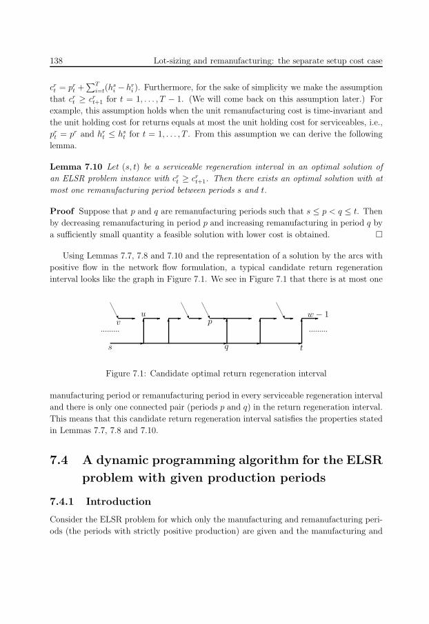
148

138 Lot-sizing and remanufacturing: the separate setup cost case

crt = pr

t +∑T

i=t(hsi − hr

i ). Furthermore, for the sake of simplicity we make the assumption

that crt ≥ cr

t+1 for t = 1, . . . , T − 1. (We will come back on this assumption later.) For

example, this assumption holds when the unit remanufacturing cost is time-invariant and

the unit holding cost for returns equals at most the unit holding cost for serviceables, i.e.,

prt = pr and hr

t ≤ hst for t = 1, . . . , T . From this assumption we can derive the following

lemma.

Lemma 7.10 Let (s, t) be a serviceable regeneration interval in an optimal solution of

an ELSR problem instance with crt ≥ cr

t+1. Then there exists an optimal solution with at

most one remanufacturing period between periods s and t.

Proof Suppose that p and q are remanufacturing periods such that s ≤ p < q ≤ t. Then

by decreasing remanufacturing in period p and increasing remanufacturing in period q by

a sufficiently small quantity a feasible solution with lower cost is obtained.

Using Lemmas 7.7, 7.8 and 7.10 and the representation of a solution by the arcs with

positive flow in the network flow formulation, a typical candidate return regeneration

interval looks like the graph in Figure 7.1. We see in Figure 7.1 that there is at most one

-

6-

6-

-

vU

-

UU -- U

q

6- --

-

6-

......... .........

-

ts

w − 1p

u6

Figure 7.1: Candidate optimal return regeneration interval

manufacturing period or remanufacturing period in every serviceable regeneration interval

and there is only one connected pair (periods p and q) in the return regeneration interval.

This means that this candidate return regeneration interval satisfies the properties stated

in Lemmas 7.7, 7.8 and 7.10.

7.4 A dynamic programming algorithm for the ELSR

problem with given production periods

7.4.1 Introduction

Consider the ELSR problem for which only the manufacturing and remanufacturing peri-

ods (the periods with strictly positive production) are given and the manufacturing and

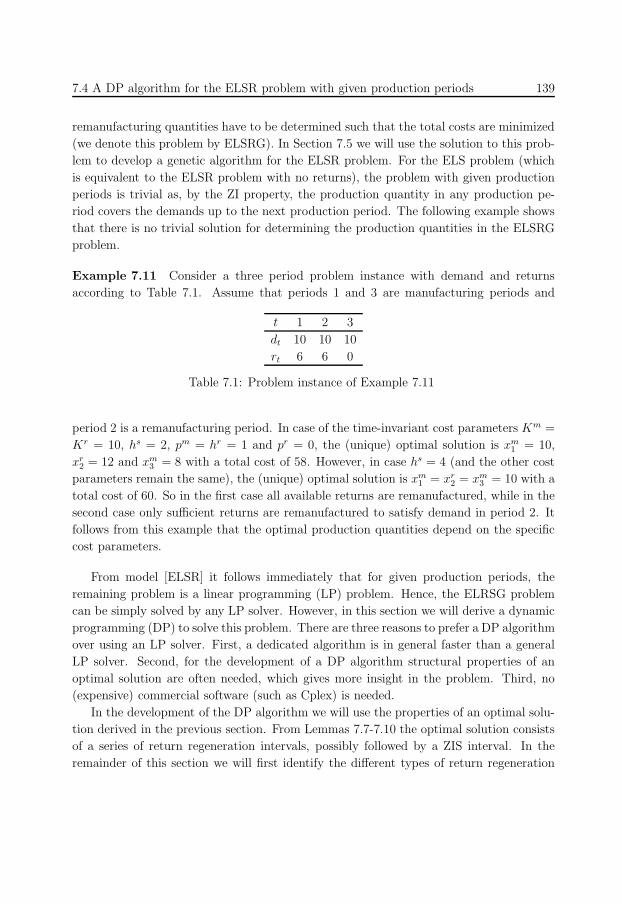
149

7.4 A DP algorithm for the ELSR problem with given production periods 139

remanufacturing quantities have to be determined such that the total costs are minimized

(we denote this problem by ELSRG). In Section 7.5 we will use the solution to this prob-

lem to develop a genetic algorithm for the ELSR problem. For the ELS problem (which

is equivalent to the ELSR problem with no returns), the problem with given production

periods is trivial as, by the ZI property, the production quantity in any production pe-

riod covers the demands up to the next production period. The following example shows

that there is no trivial solution for determining the production quantities in the ELSRG

problem.

Example 7.11 Consider a three period problem instance with demand and returns

according to Table 7.1. Assume that periods 1 and 3 are manufacturing periods and

t 1 2 3

dt 10 10 10

rt 6 6 0

Table 7.1: Problem instance of Example 7.11

period 2 is a remanufacturing period. In case of the time-invariant cost parameters Km =

Kr = 10, hs = 2, pm = hr = 1 and pr = 0, the (unique) optimal solution is xm1 = 10,

xr2 = 12 and xm

3 = 8 with a total cost of 58. However, in case hs = 4 (and the other cost

parameters remain the same), the (unique) optimal solution is xm1 = xr

2 = xm3 = 10 with a

total cost of 60. So in the first case all available returns are remanufactured, while in the

second case only sufficient returns are remanufactured to satisfy demand in period 2. It

follows from this example that the optimal production quantities depend on the specific

cost parameters.

From model [ELSR] it follows immediately that for given production periods, the

remaining problem is a linear programming (LP) problem. Hence, the ELRSG problem

can be simply solved by any LP solver. However, in this section we will derive a dynamic

programming (DP) to solve this problem. There are three reasons to prefer a DP algorithm

over using an LP solver. First, a dedicated algorithm is in general faster than a general

LP solver. Second, for the development of a DP algorithm structural properties of an

optimal solution are often needed, which gives more insight in the problem. Third, no

(expensive) commercial software (such as Cplex) is needed.

In the development of the DP algorithm we will use the properties of an optimal solu-

tion derived in the previous section. From Lemmas 7.7-7.10 the optimal solution consists

of a series of return regeneration intervals, possibly followed by a ZIS interval. In the

remainder of this section we will first identify the different types of return regeneration

150

140 Lot-sizing and remanufacturing: the separate setup cost case

intervals, where the types depend on the periods for which demand is satisfied. Sub-

sequently, we will show how to calculate the costs for these intervals and for the ZIS

intervals. Finally, we will give the recursion formulas of the DP algorithm.

7.4.2 The different types of regeneration intervals

First, we will start with identifying the different types of return regeneration intervals.

Therefore, we will need some additional notation:

P M : the set of manufacturing periods,

P R: the set of remanufacturing periods including an artificial remanufacturing period 0,

P R(t): the remanufacturing periods before period t, i.e., P R(t) = s ∈ P R : s < t,

σR(t): the remanufacturing period succeeding period t or period t itself if it is a remanu-

facturing period (T + 1 if the period does not exist),

σ(t): the production period succeeding period t or period t itself if it is a production

period (T + 1 if the period does not exist).

By adding the artificial remanufacturing period 0, period 1 is by definition a return

regeneration period. Furthermore, we add a subscript “+” to the definitions σR(t), σ(t)

when we exclude period t. (So σR(t) = mins ∈ P R : s ≥ t and σR+(t) = mins ∈ P R :

s > t.)Given the set P R, we will now identify different types of candidate regeneration inter-

vals. Let r and t (r < t) be two remanufacturing periods. Then (s, t) with s = r + 1 is

a candidate return regeneration interval. By definition of a return regeneration interval,

the returns in periods [s, t] (Rs,t) are completely remanufactured to satisfy demand. To

calculate the cost corresponding to a return regeneration interval, we have to determine

which demands are satisfied by remanufacturing and by manufacturing. Furthermore, to

construct a feasible (forward) DP algorithm, we have to include the demands that are

satisfied by manufacturing in the return regeneration intervals in such a way that a series

of return regeneration intervals covers a consecutive series of demands (starting at pe-

riod 1). Therefore, we define the following periods corresponding to a return regeneration

interval (s, t) (see also Figure 7.1):

u: the next remanufacturing period after period s, i.e., u = σR(s),

v: the next production period after period s, i.e., v = σ(s),

w: the next production period after t, i.e., w = σ+(t).

151

7.4 A DP algorithm for the ELSR problem with given production periods 141

Note that for given remanufacturing periods s and t, the periods u, v and w are uniquely

specified and satisfy s ≤ v ≤ u ≤ t < w. For notational convenience we do not show

the dependency of the periods u, v and w on periods s and t. We define the following

variables corresponding to the different types of return regeneration intervals, which will

be used in the DP algorithm:

f 00s,t: minimum cost for regeneration interval (s, t), where demands in periods [v, w − 1]

are satisfied and Isv−1 = Is

w−1 = 0 (∞ if infeasible),

f 01s,t: minimum cost for regeneration interval (s, t), where demands in periods [v, σ+(w)−1]

are satisfied and Isv−1 = 0 and Is

w > 0 (∞ if infeasible),

f 10s,t: minimum cost for regeneration interval (s, t), where demands in periods [σ+(v), w−1]

are satisfied and Isv−1 > 0 and Is

w−1 = 0 (∞ if infeasible),

f 11s,t: minimum cost for regeneration interval (s, t), where demands in periods [σ+(v), σ+(w)−

1] are satisfied and Isv−1 > 0 and Is

w > 0 (∞ if infeasible).

From the definitions it follows that we have four types (00, 01, 10 and 11) of return

regeneration intervals. Note that the candidate regeneration interval of Figure 7.1 is of

type 00. From the definition of type 00 it follows that the cost of manufacturing between

periods s and u (if any) are also included. Furthermore, for a type 00 regeneration interval

period v is the start of a serviceable regeneration interval and period w − 1 is the end

of a serviceable regeneration interval. By Lemma 7.8 it follows that there is at most one

connected pair within periods [v, w − 1].

The place where the connected pair occurs in the (previous) regeneration interval

determines the type of regeneration interval. In Figure 7.2 all types of regeneration

intervals are illustrated. Note that for a given regeneration interval (s, t) not all types

may be defined. For example, type 01 does not exist if the production period after w is

a remanufacturing period. In this case we set the cost of such a regeneration interval to

infinity.

Furthermore, given the type of regeneration interval, the demand periods to be covered

are known. This information can be used to determine whether there is an RM or MR

connection. Assume for the moment that the regeneration interval satisfies the ZI property

for serviceables. Then the total quantity of items being remanufactured to satisfy demand

equals

x =∑

i∈P R:s≤i≤t

Di,σ+(i)−1. (7.1)

If Rs,t > x, then there are some returns left that can be used to (partially) satisfy demand

periods which are satisfied by manufacturing. This means that we must have a RM

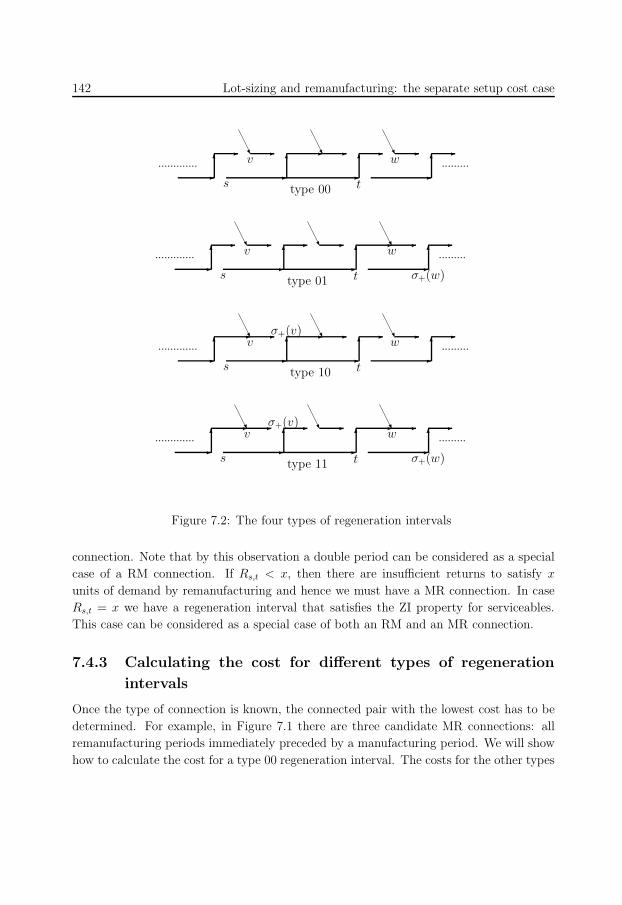
152

142 Lot-sizing and remanufacturing: the separate setup cost case

-6

-

-6

U U -

-6

U

-6

-............. .........

s t

v w- - - -

type 00

-6

-

-6

U U -

-6

U

-6

-............. .........

s t

v w- - - -

type 01 σ+(w)

-6

-

-6

U U -

-6

U

-6

-............. .........

s t

v w- - - -

type 10

σ+(v)

-6

-

-6

U U -

-6

U

-6

-............. .........

s t

v w- - - -

σ+(w)type 11

σ+(v)

Figure 7.2: The four types of regeneration intervals

connection. Note that by this observation a double period can be considered as a special

case of a RM connection. If Rs,t < x, then there are insufficient returns to satisfy x

units of demand by remanufacturing and hence we must have a MR connection. In case

Rs,t = x we have a regeneration interval that satisfies the ZI property for serviceables.

This case can be considered as a special case of both an RM and an MR connection.

7.4.3 Calculating the cost for different types of regeneration

intervals

Once the type of connection is known, the connected pair with the lowest cost has to be

determined. For example, in Figure 7.1 there are three candidate MR connections: all

remanufacturing periods immediately preceded by a manufacturing period. We will show

how to calculate the cost for a type 00 regeneration interval. The costs for the other types

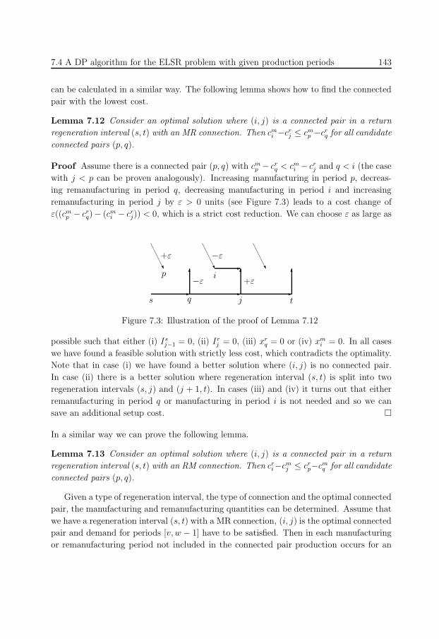
153

7.4 A DP algorithm for the ELSR problem with given production periods 143

can be calculated in a similar way. The following lemma shows how to find the connected

pair with the lowest cost.

Lemma 7.12 Consider an optimal solution where (i, j) is a connected pair in a return

regeneration interval (s, t) with an MR connection. Then cmi −cr

j ≤ cmp −cr

q for all candidate

connected pairs (p, q).

Proof Assume there is a connected pair (p, q) with cmp − cr

q < cmi − cr

j and q < i (the case

with j < p can be proven analogously). Increasing manufacturing in period p, decreas-

ing remanufacturing in period q, decreasing manufacturing in period i and increasing

remanufacturing in period j by ε > 0 units (see Figure 7.3) leads to a cost change of

ε((cmp − cr

q)− (cmi − cr

j)) < 0, which is a strict cost reduction. We can choose ε as large as

-

6U

-

6U -

-

6U

p

q

i

j

+ε −ε

−ε +ε

ts

Figure 7.3: Illustration of the proof of Lemma 7.12

possible such that either (i) Isj−1 = 0, (ii) Ir

j = 0, (iii) xrq = 0 or (iv) xm

i = 0. In all cases

we have found a feasible solution with strictly less cost, which contradicts the optimality.

Note that in case (i) we have found a better solution where (i, j) is no connected pair.

In case (ii) there is a better solution where regeneration interval (s, t) is split into two

regeneration intervals (s, j) and (j + 1, t). In cases (iii) and (iv) it turns out that either

remanufacturing in period q or manufacturing in period i is not needed and so we can

save an additional setup cost.

In a similar way we can prove the following lemma.

Lemma 7.13 Consider an optimal solution where (i, j) is a connected pair in a return

regeneration interval (s, t) with an RM connection. Then cri−cm

j ≤ crp−cm

q for all candidate

connected pairs (p, q).

Given a type of regeneration interval, the type of connection and the optimal connected

pair, the manufacturing and remanufacturing quantities can be determined. Assume that

we have a regeneration interval (s, t) with a MR connection, (i, j) is the optimal connected

pair and demand for periods [v, w − 1] have to be satisfied. Then in each manufacturing

or remanufacturing period not included in the connected pair production occurs for an

154

144 Lot-sizing and remanufacturing: the separate setup cost case

integral number of periods up to the next production period as these periods satisfy the ZI

property for serviceables. Furthermore, in period i, besides manufacturing for an integral

number of periods up to remanufacturing period j, manufacturing an additional quantity

y = x − Rs,t (with x defined in (7.1)) is necessary to compensate for the shortage of

returns and we can remanufacture y items less in period j. So the production quantities

become

xmt =

Dt,σ+(t)−1 if t ∈ P M\i ∩ [v, w − 1]

Dt,σ+(t)−1 + y if t = i,

xrt =

Dt,σ+(t)−1 if t ∈ P R\j ∩ [v, w − 1]

Dt,σ+(t)−1 − y if t = j.

Using similar arguments, the production quantities for a RM connection with a connected

pair (i, j) are

xmt =

Dt,σ+(t)−1 if t ∈ P M\j ∩ [v, w − 1]

Dt,σ+(t)−1 − y if t = j,

xrt =

Dt,σ+(t)−1 if t ∈ P R\i ∩ [v, w − 1]

Dt,σ+(t)−1 + y if t = i

with y = Rs,t − x.

Given a type of regeneration interval, the type of connection, the optimal connected

pair and the manufacturing and remanufacturing quantities, the optimal cost for a re-

generation interval can now be calculated. However, first we have to check whether we

have a feasible solution for the regeneration interval. That is, we have to check whether

xmt ≥ 0, xr

t ≥ 0, Irt ≥ 0 and Is

t ≥ 0 for t ∈ [v, w − 1]. By allowing that Irt ≥ 0 (instead

of Irt > 0 according to the definition of a return regeneration interval), it may be that

a regeneration interval consists of multiple regeneration intervals where at most one re-

generation interval has a connected pair and the other regeneration intervals satisfy the

ZI property for serviceables. Therefore, we do not need additional variables representing

the costs of return regeneration intervals satisfying the ZI property for serviceables. If no

feasible solution exists, we set the cost to infinity. Otherwise the cost is calculated by

f 00s,t =

t∑

i=s

(Kmt δ(xm

t ) + cmt xm

t + Krt δ(x

rt ) + cr

txrt ) .

For a given regeneration interval it takes O(T ) time to find the optimal connected pair,

to perform the feasibility check and to calculate the cost. As there are O(T 2) possible

regeneration intervals, the computation time for determining all values fα,βs,t (s, t ∈ P R

and α, β ∈ 0, 1) takes O(T 3) time.

We end this section with some remarks. If we have a regeneration interval with

a RM (MR) connection and there is no manufacturing period immediately preceding

155

7.4 A DP algorithm for the ELSR problem with given production periods 145

(succeeding) a remanufacturing period, then we set the cost to infinity. Furthermore, if

we have a regeneration interval of type 01 or 11, then the connected pair is immediately

known and does not have to be searched for. Similarly, if the regeneration interval includes

a double period, then it is also not necessary to search for the connected pair and the

type 01 and 11 regeneration interval do not exist as a return regeneration interval has at

most one connected pair. Finally, we come back to the assumption that crt ≥ cr

t+1. By

this property it followed from Lemma 7.10 that for any two consecutive remanufacturing

periods p and q it always holds that Irq−1 = 0 in an optimal solution. If we relax this

assumption we either have Irp = 0 or Ir

q−1 = 0 (see also Section 6.3). This case can be

easily incorporated into the DP algorithm. However, to avoid additional notation and to

keep things concise we have not included this case.

7.4.4 The interval that satisfies the ZI property for serviceables

By Lemma 7.9 we know that an optimal solution may end with an ZIS interval. In this

section we show how to calculate the cost for such an interval. Let s ∈ P R, t = s + 1,

v = σ(t) and

g0t : minimum cost for ZIS interval where returns in [t, T ] are used to satisfy demand in

periods [v, T ] (∞ if infeasible),

g1t : minimum cost for ZIS interval where returns in [t, T ] are used to satisfy demand in

periods [σ+(v), T ] (∞ if infeasible).

Again we need two types of intervals as an ZIS interval may be preceded by either a

type 00 or 10 regeneration interval or a type 01 or 11 regeneration interval (see also

Section 7.4.5). For a type 0 ZIS interval the production quantities are determined by

xmi = Di,σ+(i)−1 if i ∈ P M ∩ [v, T ],

xri = Di,σ+(i)−1 if i ∈ P R ∩ [v, T ],

because (by definition) the interval satisfies the ZI for serviceables. After checking feasi-

bility the cost is calculated by

g0t =

T∑

i=v

(Kmt δ(xm

t ) + cmt xm

t + Krt δ(x

rt ) + cr

txrt ) .

In a similar way the production quantities and cost for a type 1 ZIS interval can be

calculated. (Note that g0t = g1

t = 0 if v = T + 1.) For a given t = s + 1 with s ∈ P R it

takes O(T ) time to calculate the cost and to perform the feasibility check. As there are

O(T ) possible values of t, it takes O(T 2) time to calculate all values gαt (t = s + 1 with

s ∈ P R and α ∈ 0, 1).

156

146 Lot-sizing and remanufacturing: the separate setup cost case

7.4.5 The recursion formulas

From Lemmas 7.7-7.9 it follows that an optimal solution consists of a series of regeneration

intervals (possibly followed by a ZIS interval). Therefore, we define the variables fαt with

t ∈ P R and α ∈ 0, 1 as follows:

f 0t : minimum cost to satisfy demand in periods [1, w − 1] with w = σ+(t),

f 1t : minimum cost to satisfy demand in periods [1, σ+(w) − 1] with w = σ+(t).

So f 0t is the cost of a partial solution consisting of a series of return regeneration intervals

ending with a type 00 or 10 regeneration interval and f 1t is the cost of a partial solution

ending with a type 01 or 11 regeneration interval. Starting with f 00 = 0 and f 1

0 = ∞ the

values of fαt can be calculated by

fαt = min

s∈P R(t)

min

β∈0,1

fβ

s + fβ,αs+1,t

for all t ∈ P R\0, α ∈ 0, 1. (7.2)

Note that a type 0 (1) partial solution must be followed by a type 00 or 01 (10 or 11)

regeneration interval. Because the series of regeneration intervals may be followed by a

ZIS interval the optimal cost f ∗ is found by

f ∗ = mins∈P R

min

α∈0,1

fα

s + gαs+1

. (7.3)

Again a type 0 (1) partial solution has to be followed by a type 0 (1) ZIS interval. It is not

difficult to see from (7.2) and (7.3) that it takes O(T 2) and O(T ) and time to calculate

the values fαt (t ∈ P R, α ∈ 0, 1) and f ∗, respectively. Furthermore, as it takes O(T 3)

and O(T 2) to calculate fβ,αs+1,t and gα

s+1, respectively (see Sections 7.4.3 and 7.4.4), we have

the following theorem.

Theorem 7.14 The ELSRG problem can be solved in O(T 3) time.

7.5 Application of the DP algorithm to a genetic al-

gorithm

In Section 7.2 we have shown that the ELSR problem is NP-hard and hence it is very

unlikely that there exists an efficient algorithm to solve the problem. In this section we

will propose a genetic algorithm (GA) to find good solutions. First, we will describe the

algorithm and then we will present some numerical results. We propose a straightforward

GA such that only a few parameters have to be specified. In this way we try to avoid the

need to ‘fine-tune’ the algorithm in such a way that it performs well on our specific data

set.

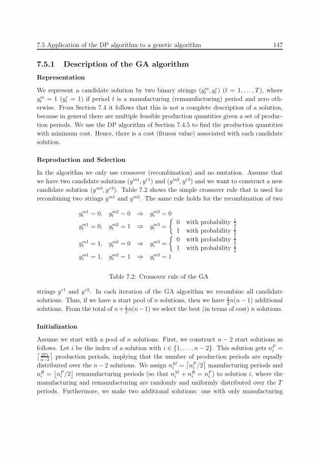
157

7.5 Application of the DP algorithm to a genetic algorithm 147

7.5.1 Description of the GA algorithm

Representation

We represent a candidate solution by two binary strings (ymt , yr

t ) (t = 1, . . . , T ), where

ymt = 1 (yr

t = 1) if period t is a manufacturing (remanufacturing) period and zero oth-

erwise. From Section 7.4 it follows that this is not a complete description of a solution,

because in general there are multiple feasible production quantities given a set of produc-

tion periods. We use the DP algorithm of Section 7.4.5 to find the production quantities

with minimum cost. Hence, there is a cost (fitness value) associated with each candidate

solution.

Reproduction and Selection

In the algorithm we only use crossover (recombination) and no mutation. Assume that

we have two candidate solutions (ym1, yr1) and (ym2, yr2) and we want to construct a new

candidate solution (ym3, yr3). Table 7.2 shows the simple crossover rule that is used for

recombining two strings ym1 and ym2. The same rule holds for the recombination of two

ym1t = 0, ym2

t = 0 ⇒ ym3t = 0

ym1t = 0, ym2

t = 1 ⇒ ym3t =

0 with probability 1

2

1 with probability 12

ym1t = 1, ym2

t = 0 ⇒ ym3t =

0 with probability 1

2

1 with probability 12

ym1t = 1, ym2

t = 1 ⇒ ym3t = 1

Table 7.2: Crossover rule of the GA

strings yr1 and yr2. In each iteration of the GA algorithm we recombine all candidate

solutions. Thus, if we have a start pool of n solutions, then we have 12n(n− 1) additional

solutions. From the total of n+ 12n(n−1) we select the best (in terms of cost) n solutions.

Initialization

Assume we start with a pool of n solutions. First, we construct n − 2 start solutions as

follows. Let i be the index of a solution with i ∈ 1, . . . , n − 2. This solution gets nPi =⌈

2T in−2

⌉production periods, implying that the number of production periods are equally

distributed over the n− 2 solutions. We assign nMi =

⌈nP

i /2⌉

manufacturing periods and

nRi =

⌊nP

i /2⌋

remanufacturing periods (so that nMi + nR

i = nPi ) to solution i, where the

manufacturing and remanufacturing are randomly and uniformly distributed over the T

periods. Furthermore, we make two additional solutions: one with only manufacturing

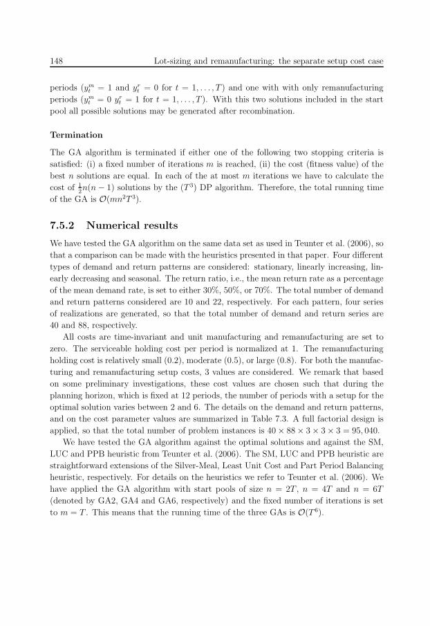
158

148 Lot-sizing and remanufacturing: the separate setup cost case

periods (ymt = 1 and yr

t = 0 for t = 1, . . . , T ) and one with with only remanufacturing

periods (ymt = 0 yr

t = 1 for t = 1, . . . , T ). With this two solutions included in the start

pool all possible solutions may be generated after recombination.

Termination

The GA algorithm is terminated if either one of the following two stopping criteria is

satisfied: (i) a fixed number of iterations m is reached, (ii) the cost (fitness value) of the

best n solutions are equal. In each of the at most m iterations we have to calculate the

cost of 12n(n − 1) solutions by the (T 3) DP algorithm. Therefore, the total running time

of the GA is O(mn2T 3).

7.5.2 Numerical results

We have tested the GA algorithm on the same data set as used in Teunter et al. (2006), so

that a comparison can be made with the heuristics presented in that paper. Four different

types of demand and return patterns are considered: stationary, linearly increasing, lin-

early decreasing and seasonal. The return ratio, i.e., the mean return rate as a percentage

of the mean demand rate, is set to either 30%, 50%, or 70%. The total number of demand

and return patterns considered are 10 and 22, respectively. For each pattern, four series

of realizations are generated, so that the total number of demand and return series are

40 and 88, respectively.

All costs are time-invariant and unit manufacturing and remanufacturing are set to

zero. The serviceable holding cost per period is normalized at 1. The remanufacturing

holding cost is relatively small (0.2), moderate (0.5), or large (0.8). For both the manufac-

turing and remanufacturing setup costs, 3 values are considered. We remark that based

on some preliminary investigations, these cost values are chosen such that during the

planning horizon, which is fixed at 12 periods, the number of periods with a setup for the

optimal solution varies between 2 and 6. The details on the demand and return patterns,

and on the cost parameter values are summarized in Table 7.3. A full factorial design is

applied, so that the total number of problem instances is 40 × 88 × 3 × 3 × 3 = 95, 040.

We have tested the GA algorithm against the optimal solutions and against the SM,

LUC and PPB heuristic from Teunter et al. (2006). The SM, LUC and PPB heuristic are

straightforward extensions of the Silver-Meal, Least Unit Cost and Part Period Balancing

heuristic, respectively. For details on the heuristics we refer to Teunter et al. (2006). We

have applied the GA algorithm with start pools of size n = 2T , n = 4T and n = 6T

(denoted by GA2, GA4 and GA6, respectively) and the fixed number of iterations is set

to m = T . This means that the running time of the three GAs is O(T 6).

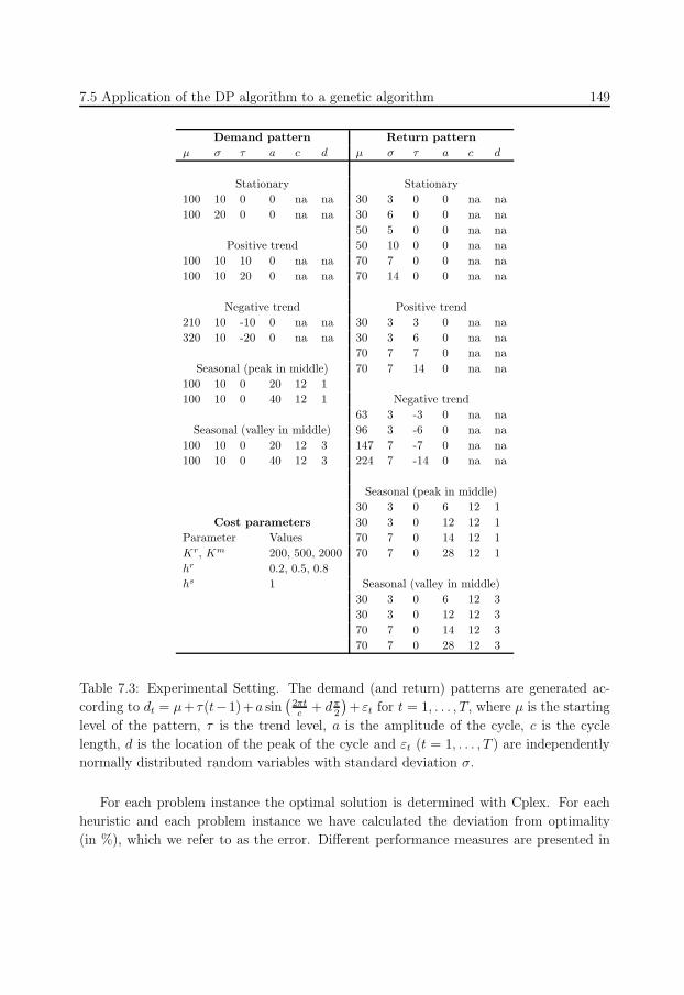
159

7.5 Application of the DP algorithm to a genetic algorithm 149

Demand pattern Return pattern

µ σ τ a c d µ σ τ a c d

Stationary Stationary

100 10 0 0 na na 30 3 0 0 na na

100 20 0 0 na na 30 6 0 0 na na

50 5 0 0 na na

Positive trend 50 10 0 0 na na

100 10 10 0 na na 70 7 0 0 na na

100 10 20 0 na na 70 14 0 0 na na

Negative trend Positive trend

210 10 -10 0 na na 30 3 3 0 na na

320 10 -20 0 na na 30 3 6 0 na na

70 7 7 0 na na

Seasonal (peak in middle) 70 7 14 0 na na

100 10 0 20 12 1

100 10 0 40 12 1 Negative trend

63 3 -3 0 na na

Seasonal (valley in middle) 96 3 -6 0 na na

100 10 0 20 12 3 147 7 -7 0 na na

100 10 0 40 12 3 224 7 -14 0 na na

Seasonal (peak in middle)

30 3 0 6 12 1

Cost parameters 30 3 0 12 12 1

Parameter Values 70 7 0 14 12 1

Kr, Km 200, 500, 2000 70 7 0 28 12 1

hr 0.2, 0.5, 0.8

hs 1 Seasonal (valley in middle)

30 3 0 6 12 3

30 3 0 12 12 3

70 7 0 14 12 3

70 7 0 28 12 3

Table 7.3: Experimental Setting. The demand (and return) patterns are generated ac-

cording to dt = µ+ τ(t−1)+a sin(

2πtc

+ dπ2

)+ εt for t = 1, . . . , T, where µ is the starting

level of the pattern, τ is the trend level, a is the amplitude of the cycle, c is the cycle

length, d is the location of the peak of the cycle and εt (t = 1, . . . , T ) are independently

normally distributed random variables with standard deviation σ.

For each problem instance the optimal solution is determined with Cplex. For each

heuristic and each problem instance we have calculated the deviation from optimality

(in %), which we refer to as the error. Different performance measures are presented in

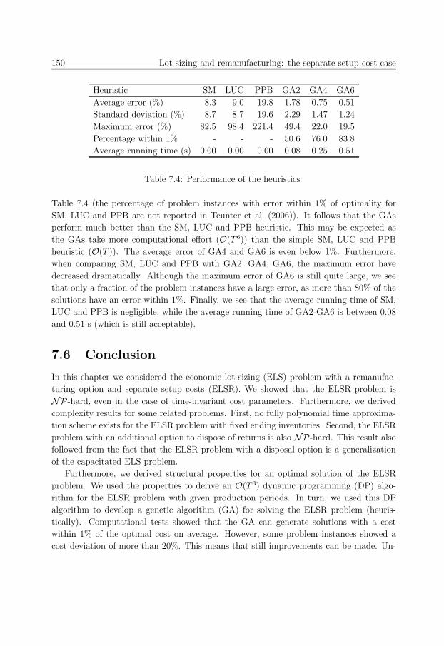
160

150 Lot-sizing and remanufacturing: the separate setup cost case

Heuristic SM LUC PPB GA2 GA4 GA6

Average error (%) 8.3 9.0 19.8 1.78 0.75 0.51

Standard deviation (%) 8.7 8.7 19.6 2.29 1.47 1.24

Maximum error (%) 82.5 98.4 221.4 49.4 22.0 19.5

Percentage within 1% - - - 50.6 76.0 83.8

Average running time (s) 0.00 0.00 0.00 0.08 0.25 0.51

Table 7.4: Performance of the heuristics

Table 7.4 (the percentage of problem instances with error within 1% of optimality for

SM, LUC and PPB are not reported in Teunter et al. (2006)). It follows that the GAs

perform much better than the SM, LUC and PPB heuristic. This may be expected as

the GAs take more computational effort (O(T 6)) than the simple SM, LUC and PPB

heuristic (O(T )). The average error of GA4 and GA6 is even below 1%. Furthermore,

when comparing SM, LUC and PPB with GA2, GA4, GA6, the maximum error have

decreased dramatically. Although the maximum error of GA6 is still quite large, we see

that only a fraction of the problem instances have a large error, as more than 80% of the

solutions have an error within 1%. Finally, we see that the average running time of SM,

LUC and PPB is negligible, while the average running time of GA2-GA6 is between 0.08

and 0.51 s (which is still acceptable).

7.6 Conclusion

In this chapter we considered the economic lot-sizing (ELS) problem with a remanufac-

turing option and separate setup costs (ELSR). We showed that the ELSR problem is

NP-hard, even in the case of time-invariant cost parameters. Furthermore, we derived

complexity results for some related problems. First, no fully polynomial time approxima-

tion scheme exists for the ELSR problem with fixed ending inventories. Second, the ELSR

problem with an additional option to dispose of returns is also NP-hard. This result also

followed from the fact that the ELSR problem with a disposal option is a generalization

of the capacitated ELS problem.

Furthermore, we derived structural properties for an optimal solution of the ELSR

problem. We used the properties to derive an O(T 3) dynamic programming (DP) algo-

rithm for the ELSR problem with given production periods. In turn, we used this DP

algorithm to develop a genetic algorithm (GA) for solving the ELSR problem (heuris-

tically). Computational tests showed that the GA can generate solutions with a cost

within 1% of the optimal cost on average. However, some problem instances showed a

cost deviation of more than 20%. This means that still improvements can be made. Un-

161

7.6 Conclusion 151

fortunately, the GA algorithm does not provide a performance guarantee on the quality

of the solutions. Therefore, an issue for future research is to find heuristics with such a

performance guarantee.

162

163

Chapter 8

Summary of the main results

In Chapter 2 we derived a new property for an optimal solution of the economic lot-sizing

(ELS) problem with time-invariant cost parameters. In this chapter we were interested in

the proportion of order cost and holding cost in an optimal solution. Let an order interval

be defined as the consecutive number of periods for which demand is satisfied by a single

order. We showed that the ratio between the total holding cost and order cost in an order

interval can be arbitrarily large. However, the ratio only increases proportionally to the

logarithm of the number of periods in the order interval. Furthermore, we showed by an

example that this bound is tight. This result is in contrast with the classical economic

order quantity (EOQ) model, where setup cost and holding cost are perfectly balanced in

an optimal solution.

The analysis resulted in the construction of a new heuristic. The main idea of the

heuristic is that a new order is started when adding an additional order to the current

order interval decreases the cost. We showed that this heuristic has worst case ratio 2.

Furthermore, we also showed that a solution generated by this heuristic has a nice theoret-

ical property: the number of setups of the heuristic solution equals at most the number of

setups generated by the optimal solution and equals at least half of this number. Finally,

we showed that the worst case ratio tends to 34

√2 in case of time-invariant demand and

sufficiently large setup cost.

In Chapter 3 we analyzed the worst case performance for a general class of on-line lot-

sizing heuristics. The class of heuristics satisfied the following properties: (i) decisions are

made on a period-by-period basis, (ii) decisions only depend on the cost of the current lot-

size, (iii) the decision rule is deterministic. We showed that heuristics satisfying (i) have

a worst case ratio of at least 32, even if the optimal solution and the heuristic solution

have at most 2 setups (including the setup in the first period). Using the analysis to

construct the worst case examples enabled us to find heuristics with optimal worst case

performance for three- and four-period problem instances.

164

154 Lot-sizing and remanufacturing: the separate setup cost case

Furthermore, we showed that heuristics satisfying (i)–(iii) have worst case ratio at

least 2. This generalizes the work of Axsater (1985), who proved this result for a more

restrictive class of heuristics. The problem instance with this performance ratio was found

by formulating the problem of finding a worst case example as a mixed inter programming

problem. As far as we know no heuristics satisfying (i) and having worst case ratio smaller

than 2 exist. This leaves an issue for further research.

In Chapter 4 we extended the ELS problem to account for pricing decisions. We consid-

ered a joint pricing and lot-sizing problem, where prices were allowed to vary over time. We

focused on a special case with a time-invariant demand function and time-invariant cost

parameters considered by Bhattacharjee and Ramesh (2000). Bhattacharjee and Ramesh

(2000) proposed two heuristics for the problem. However, we showed that by applying

existing results in the literature, the problem can be solved to optimality. Application

of (a slight modification of) the approach by Thomas (1970) led to the development of

a (practically) efficient algorithm with a running time quadratic in the model horizon.

Moreover, applying the results on a partition problem derived by Orlin (1985) led to an

improvement in running time (although the running time was still pseudopolynomial).

In Chapter 5 we developed an exact algorithm for another type of pricing and lot-sizing

problem. In the model of Chapter 5 prices were assumed to be constant over time, in

contrast to the model of Chapter 4. We generalized the work of Kunreuther and Schrage

(1973) who proposed a heuristic for the problem. We did not only show that the problem

can be solved to optimality, but we also show that this can be done in O(T 3 log T ) time.

Moreover, we improved on the the result of Gilbert (1999), who proposed an O(T 3) for a

special case of the problem. We showed that applying our approach to this special case

leads to an O(T 2) algorithm.

In Chapter 6 we considered the ELS problem with a remanufacturing option (ELSR).

In this model we assumed that a (known) quantity of products comes back from the

customer in each period and these returned products can be remanufactured to satisfy

demand (besides regular manufacturing). In this chapter we assumed that there is a

joint setup cost for manufacturing and remanufacturing. We showed that this problem

can be solved in O(T 4) time under the assumption of time-invariant cost parameters.

We developed a dynamic programming algorithm where we utilized the ‘block’ structure

associated with an extreme point solution.

Furthermore, we showed that the problem without the manufacturing option, sufficient

returns and non-stationary cost (the ‘pure’ remanufacturing problem) can be solved in

O(T 2 log T ). Moreover, we showed that this problem is equivalent to the ELS problem

with bounded inventory. This immediately provided an O(T 2 log T ) algorithm for this

problem, which is an improvement on the O(T 3) algorithm of Love (1973). Finally, the

ELSR problem with general cost parameters and no restrictions on the returns is not

known to be polynomially solvable or NP-hard. So this is an issue for future research.

165

155

In Chapter 7 again we considered the ELSR problem. However, in the model of this

chapter we assumed a separate setup cost for both manufacturing and remanufacturing,

in contrast to the model of Chapter 6. We showed that this ELSR problem is NP-hard,

even in the case of time-invariant cost parameters. This immediately proved that the

ELSR problem with an additional option to dispose of returns is NP-hard (this problem

was considered by Golany et al. (2001) and Yang et al. (2005)). Furthermore, we showed

that the ELSR problem with a disposal option is a generalization of the capacitated ELS

problem, which also proved the above result. Finally, we showed that no fully polynomial

time approximation scheme exists for the ELSR problem with fixed ending inventories,

unless P = NP.

In the remainder of Chapter 7 we derived structural properties for an optimal solution

of the ELSR problem with separate setup costs. We used the properties to derive an

O(T 3) dynamic programming (DP) algorithm for the ELSR problem with given produc-

tion periods. In turn, we used this DP algorithm to develop a genetic algorithm (GA)

for solving the ELSR problem (heuristically). Computational tests showed that the GA

can generate solutions with a cost within 1% of the optimal cost on average. However,

some problem instances showed a cost deviation of more than 20%. This means that still

improvements can be made. Unfortunately, the GA algorithm does not provide a perfor-

mance guarantee on the quality of the solutions. Therefore, an issue for future research

is to find heuristics with such a performance guarantee.

166

167

Nederlandse samenvatting

(Summary in Dutch)

Een manier waarop bedrijven kosten kunnen reduceren is efficiente productieplanning.

Het centrale thema in dit proefschrift is een klassiek productieplanningsprobleem: het

economische lot-sizing (ELS) probleem (Wagner and Whitin, 1958). Het probleem kan

als volgt worden beschreven. Er is een producent met een (bekend veronderstelde) vraag

naar een bepaald product voor een eindige, discrete planningshorizon. Er moet een pro-

ductieschema worden gevonden die in de vraag voorziet en waarbij de totale kosten worden

geminimaliseerd. Deze kosten bestaan uit: setupkosten (voor elke periode dat er wordt

geproduceerd), productiekosten (voor elk product dat wordt geproduceerd) en voorraad-

kosten (voor elk product dat in voorraad wordt gehouden).

In dit proefschrift bekijken we zowel aspecten rondom het klassieke probleem als uit-

breidingen op het probleem. In Deel I houden we ons bezig met aspecten rondom het

klassieke probleem en in Deel II and III bekijken we een aantal uitbreidingen op het ELS

model.

In Hoofdstuk 2 van dit proefschrift zijn we geınteresseerd in de eigenschappen van

een optimale oplossing voor het ELS probleem met constante kostenparameters. In het

bijzonder analyseren we de verhouding tussen de voorraadkosten en setupkosten. Deze

kosten zijn namelijk gelijk in een optimale oplossing voor het economic order quantity

(EOQ) model, een model dat nauw samenhangt met het ELS model. De vraag is nu of

deze eigenschap ook in zekere mate geldt voor het ELS probleem. Ons onderzoek laat zien

dat de verhouding tussen de setup- en voorraadkosten willekeurig groot kan zijn in een

productie-interval. (Een productie-interval is gedefinieerd als een geheel aantal periodes

waarvoor de vraag wordt voldaan door een enkele productieperiode.) De voorraadkosten

nemen echter slechts toe met een factor die proportioneel is met de setupkosten en de

logaritme van het aantal periodes in het productie-interval.

Onze analyse resulteerde in de ontwikkeling van een nieuwe heuristiek voor het ELS

probleem. In de heuristiek wordt een productie-interval zo gekozen dat het aantal periodes

in het interval zo groot mogelijk is en toevoegen van een extra productieperiode niet tot

een kostenreductie leidt. Verder heeft de heuristiek de volgende theoretische eigenschap:

168

158 Summary in Dutch

het aantal productieperiodes is ten hoogste gelijk aan het aantal productieperiodes in een

optimale oplossing en ten minste gelijk aan de helft van dit aantal. Helaas genereert de

heuristiek geen optimale oplossingen in het geval van constante vraag. In het slechtste

geval heeft de heuristiek een relatieve afwijking van 1119% en de relatieve fout convergeert

naar 34

√2 − 1(≈ 6.1%) wanneer de setupkosten willekeurig groot worden.

In Hoofdstuk 3 beschouwen we een klasse heuristieken voor het ELS probleem met

constante kostenparameters. Deze klasse bezit de volgende eigenschappen:

(i) Beslissingen worden periode voor periode genomen.

(ii) Beslissingen hangen alleen af van de kosten in het huidige productie-interval.

(iii) De beslissingsregels zijn deterministisch.

Door eigenschap (i) kan de klasse beschouwd worden als een klasse van on-line heuristie-

ken. Veel heuristieken voor het ELS probleem in de literatuur vallen binnen deze klasse.

In dit hoofdstuk zijn we geınteresseerd in de worst-case performance van deze klasse, i.e.,

de maximale afwijking van de heuristische kosten ten opzichte van de optimale kosten

(die we uitdrukken als ratio van deze twee kosten).

Ons onderzoek laat zien dat elke heuristiek binnen de bovengenoemde klasse een worst-

case ratio van ten minste 2 heeft. Dit generaliseert het resultaat van Axsater (1982), die

laat zien dat deze eigenschap geldt voor een beperktere klasse van heuristieken. Verder

laten we zien dat heuristieken die alleen aan eigenschap (i) voldoen, een worst-case ratio

van ten minste 32

hebben. Voor zover bekend bestaat er geen heuristiek die aan eigen-

schap (i) voldoet en een worst-case ratio kleiner dan 2 heeft. Dit is dus een probleem voor

verder onderzoek.

Omdat het ELS model relatief eenvoudig is, bekijken we in Deel II en III een tweetal

uitbreidingen van het klassieke ELS model. In Deel II, bestaande uit Hoofdstuk 4 en 5,

bekijken we een model waarbij het mogelijk is om de vraag te beınvloeden door middel

van het zetten van de verkoopprijs (in tegenstelling tot het klassieke model waarbij de

vraag gegeven wordt verondersteld). In Deel III, bestaande uit Hoofdstuk 6 en 7, breiden

we het model uit met een optie tot herproductie (naast reguliere productie).

In Hoofdstuk 4 bekijken we het ELS model met een mogelijkheid tot prijszetting,

waarbij de verkoopprijzen mogen varieren over de tijd. In het bijzonder richten we ons op

het model van Bhattacharjee and Ramesh (2000), die twee heuristieken ontwikkelden voor

een probleem met constante vraagfuncties. In dit hoofdstuk laten we zien dat het probleem

exact kan worden opgelost door een (praktisch) efficient algoritme door de methode van

Thomas (1970) toe te passen. Vervolgens laten we zien dat het algoritme verder kan

worden versneld door de resultaten van Orlin (1985) toe te passen.

Omdat het in sommige gevallen niet gewenst is om verschillende verkoopprijzen over

de tijd te hebben, nemen we in Hoofdstuk 5 aan dat er een prijs gezet moet worden

169

Nederlandse samenvatting 159

in alle tijdsperiodes. Kunreuther and Schrage (1973) ontwikkelden een heuristiek voor

dit probleem. Gilbert (1999) laat zien dat een speciaal geval van het probleem (exact)

opgelost kan worden in O(T 2) tijd (waarbij T de planningshorizon is). In dit hoofdstuk

verbeteren beide resultaten. Ten eerste ontwikkelen een exact algoritme voor het algemene

probleem met een looptijd van O(T 3 log T ). Ten tweede laten we zien dat de looptijd van

ons algoritme reduceert tot O(T 2) voor het model van Gilbert (1999).

In Deel III breiden we het ELS model met een mogelijkheid tot herproductie. Door

wetgeving van de overheid, het milieubewust zijn van de klant en economische redenen

nemen bedrijven steeds meer gebruikte producten (returns) terug van de klant. In ons

model nemen we aan dat deze returns kunnen worden geherproduceerd en daarna zo goed

als nieuw zijn. De vraag kan nu dus worden voldaan door zowel reguliere productie als

herproductie van returns.

In Hoofdstuk 6 nemen we aan dat er gezamenlijke setupkosten zijn voor productie

en herproductie. Dit is bijvoorbeeld het geval wanneer er een enkele productielijn voor

productie en herproductie is. We laten zien dat dit probleem efficient opgelost kan worden

in het geval van constante kostenparameters. We hebben echter niet kunnen aantonen

dat het probleem met algemene kosten NP-moeilijk of polynomiaal oplosbaar is. Dit is

dus een probleem voor verder onderzoek.

Vervolgens bekijken we een speciaal geval van het model met voldoende returns om

aan de vraag te voldoen en geen reguliere productie. We laten zien dat dit probleem kan

worden opgelost in O(T 2 log T ) tijd. Bovendien tonen we aan dat dit probleem equivalent

is aan het ELS model met capaciteiten op de hoeveelheid voorraad in elke periode. Voor

zover wij weten heeft het snelste algoritme voor dit probleem een looptijd van O(T 3)

(Love, 1973). Toepassing van ons algoritme levert dus een verbetering op.

In plaats van gezamenlijke setupkosten voor productie en herproductie nemen we in

Hoofdstuk 7 aan dat er aparte setupkosten zijn. Dit is bijvoorbeeld het geval wanneer

er aparte productielijnen voor productie en herproductie zijn. In dit hoofdstuk laten

we zien dat dit probleem NP-moeilijk is, zelfs in het geval van constante kostenpara-

meters. Verder leiden we in dit hoofdstuk complexiteitsresultaten af voor gerelateerde

problemen. Ten slotte ontwikkelen een genetisch algoritme voor het probleem. Numerie-

ke experimenten tonen aan dat de gemiddelde performance goed is (op onze verzameling

van testproblemen): de afwijking ten opzichte van het optimum ligt gemiddeld binnen 1%.

De maximale afwijking ligt echter boven 20%. Hier ligt dus nog een mogelijkheid tot ver-

betering. Verder is de ontwikkeling van een heuristiek met een performance garantie ook

een issue voor verder onderzoek.

170

171

Bibliography

A. Aggarwal and J. K. Park. Improved algorithms for economic lot-size problems. Oper-

ations Research, 14:549–571, 1993.

A. Atamturk and S. Kucukyavuz. Lot sizing with inventory bounds and fixed costs:

Polyhedral study and computation. Operations Research, 53:711–730, 2005.

S. Axsater. Worst case performance for lot sizing heuristics. European Journal of Opera-

tional Research, 9(4):339–343, 1982.

S. Axsater. Performance bounds for lot sizing heuristics. Management Science, 31:634–

640, 1985.

S. Axsater. A sequential lot sizing heuristic with optimal average performance. Manage-

ment Science, 34(11):1324–1332, 1988.

K. R. Baker. Lot-sizing procedures and a standard data set: A reconciliation of the

literature. Journal of Manufacturing and Operations Management, 2:199–221, 1989.

J. L. Beltran and D. Krass. Dynamic lot sizing with returning items and disposals. IIE

Transactions, 34(5):437–448, 2002.

S. Bhattacharjee and R. Ramesh. A multi-period profit maximizing model for retail supply

chain management: An integration of demand and supply-side mechanisms. European

Journal of Operational Research, 122:584–601, 2000.

G. R. Bitran and H. H. Yanasse. Computational complexity of the capacitated lot size

problem. Management Science, 28:1174–1186, 1982.

G. R. Bitran, T. L. Magnanti, and H. H. Yanasse. Approximation methods for the

uncapacitated lot size problem. Management Science, 30(9):1121–1140, 1984.

N. Brahimi, S. Dauzere-Peres, N. M. Najid, and A. Nordli. Single item lot sizing problems.

European Journal of Operational Research, 168(1):1–16, 2006.

172

162 Bibliography

L. M. A. Chan, A. Muriel, Z. J. Shen, and D. Simchi-Levi. On the effectiveness of zero

inventory-ordering policies for the economic lot-sizing model with a class of piecewise

linear cost structures. Operations Research, 50(6):1058–1067, 2002.

S. Chand. Lot sizing for products with finite demand horizon and periodic review inventory

police. European Journal of Operational Research, 11:145–148, 1982.

R. Dekker, M. Fleischmann, K. Inderfurth, and L. N. van Wassenhove. Reverse Logistics:

Quantitative Models for Closed-Loop Supply Chains. Springer-Verlag, Berlin Heidelberg,

2004.

A. Drexl and A. Kimms. Lot sizing and scheduling - survey and extensions. European

Journal of Operational Research, 99:221–235, 1997.

M. J. Eisner and D. G. Severance. Mathematical techniques for efficient record segmen-

tation in large shared databases. Journal of the Association for Computing Machinery,

23:619–635, 1976.

J. Eliashberg and R. Steinberg. Marketing-production joint decision making. In J. Eliash-

berg and G. Lilien, editors, Handbooks In Operations Research and Management: Mar-

keting, chapter 18, pages 827–880. Amsterdam: Elsevier Science Publishers B.V., 1993.

G. D. Eppen and R. K. Martin. Solving multi-item capacitated lot-sizing problems using

variable redefinition. Operations Research, 35(6):832–848, 1987.

A. Federgruen and J. Meissner. Competition under time-varying demands and dynamic

lot-sizing costs. Technical report, Graduate School of Business, Columbia University,

2005.

A. Federgruen and M. Tzur. A simple forward algorithm to solve general dynamic lot

sizing models with n periods in O(n log n) or O(n) time. Management Science, 37,

1991.

A. Federgruen, J. Meissner, and M. Tzur. Progressive interval heuristics for multi-item

capacitated lot sizing problems. Operations Research, 2006. (forthcoming).

M. Fisher, R. Ramdas, and Y. Zheng. Ending inventory valuation in multiperiod produc-

tion scheduling. Management Science, 5:679–692, 2001.

M. Fleischmann, J. M. Bloemhof-Ruwaard, R. Dekker, E. A. van der Laan, J. A. E. E.

van Nunen, and L. N. van Wassenhove. Quantitative models for reverse logistics: a

review. European Journal of Operational Research, 103:1–17, 1997.

173

Bibliography 163

M. Florian, J. K. Lenstra, and A. H. G. Rinnooy Kan. Deterministic production planning:

algorithms and complexity. Management Science, 26:669–679, 1980.

M. R. Garey and D. S. Johnson. Computers and Intractability: A Guide to the Theory of

NP-Completeness. W.H. Freeman and Company, New York, 1979.

J. Geunes, Y. Merzifonluoglu, and H. E. Romeijn. Capacitated procurement planning

with price-sensitive demand and general concave revenue functions. Technical report,

Department of Industrial and Systems Engineering, University of Florida, 2005.

J. Geunes, H. E. Romeijn, and K. Taaffe. Requirements planning with pricing and order

selection flexibility. Operations Research, 54(2):394–401, 2006.

S. M. Gilbert. Coordination of pricing and multiple-period production for constant priced

goods. European Journal of Operational Research, 114:330–337, 1999.

S. M. Gilbert. Coordination of pricing and multiple-period production across multiple

constant priced goods. Management Science, 46:1602–1616, 2000.

B. Golany, J. Yang, and G. Yu. Economic lot-sizing with remanufacturing options. IIE

Transactions, 33:995–1003, 2001.

F. W. Harris. How many parts to make at once. Factory, The magazine of management,

10:135–136, 1913.

R. Jans and Z. Degraeve. A new dantzig-wolfe reformulation and branch-and-price algo-

rithm for the capacitated lot sizing problem with set up times. Operations Research,

2006. (forthcoming).

R. Jans and Z. Degraeve. Modeling industrial lot sizing problems: A review. International

Journal of Production Research, 2007. (forthcoming).

R. Kuik, M. Salomon, and L. N. van Wassenhove. Batching decisions: Structure and

models. European Journal of Operational Research, 18:243–263, 1994.

H. Kunreuther and L. Schrage. Joint pricing and inventory decisions for constant priced

items. Management Science, 19:732–738, 1973.

Y. Li, J. Chen, and X. Cai. Uncapacitated production planning with multiple product

types, returned product remanufacturing, and demand substitution. OR Spectrum, 28

(1):101–125, 2006.

F. Love. Bounded production and inventory models with piecewise concave costs. Man-

agement Science, 20:313–318, 1973.

174

164 Bibliography

J. B. Orlin. Some very easy knapsack/partition problems. Operations Research, 33(5):

1154–1160, 1985.

C. H. Papadimitriou and K. Steiglitz. Combinatorial Optimization: Algorithms and Com-

plexity. Prentice-Hall, 1982.

K. Richter and M. Sombrutzki. Remanufacturing planning for the reverse Wagner/Whitin

models. European Journal of Operational Research, 121:304–315, 2000.

K. Richter and J. Weber. The reverse Wagner/Whitin model with variable manufacturing

and remanufacturing cost. International Journal of Production Economics, 71:447–456,

2001.

N. C. Simpson. Questioning the relative virtues of dynamic lot sizing rules. Computers

and Operations Research, 28:899–914, 2001.

A. G. Sogomonian and C. S. Tang. A modeling framework for coordinating promotion

and production decisions within a firm. Management Science, 39:191–203, 1993.

H. Stadtler. Improved rolling schedules for the dynamic single-level lot-sizing problem.

Management Science, 46(2):318–326, 2000.

R. H. Teunter, Z. P. Bayındır, and W. van den Heuvel. Dynamic lot sizing with product

returns and remanufacturing. International Journal of Production Research, 44(20):

4377–4400, 2006.

M. V. Thierry, M. Salomon, J. A. E. E. van Nunen, and L. N. van Wassenhove. Strategic

issues in product recovery management. California Management Review, 37:114–135,

1995.

J. Thomas. Price production decisions with deterministic demand. Management Science,

16:747–750, 1970.

R. Vachani. Performance of heuristics for the uncapacitated lot size problem. Naval

Research Logistics, 39:801–813, 1992.

W. van den Heuvel. On the complexity of the economic lot-sizing problem with remanufac-

turing options. Technical Report Report EI 2004-46, Econometric Institute, Rotterdam,

2004.

W. van den Heuvel and A. P. M. Wagelmans. A note on a multi-period profit maximizing

model for retail supply chain management. Technical Report EI 2003-36, Econometric

Institute, Erasmus University Rotterdam, 2003.

175

Bibliography 165

W. van den Heuvel and A. P. M. Wagelmans. A comparison of methods for lot-sizing in

a rolling horizon environment. Operations Research Letters, 33:486–496, 2005.

W. van den Heuvel and A. P. M. Wagelmans. An efficient dynamic programming algo-

rithm for a special case of the capacitated lot-sizing problem. Computers & Operations

Research, 33:3583–3599, 2006a.

W. van den Heuvel and A. P. M. Wagelmans. A polynomial time algorithm for a deter-

ministic joint pricing and inventory model. European Journal of Operational Research,

170:463–480, 2006b.

W. van den Heuvel, P. E. M. Borm, and H. J. M. Hamers. Economic lot-sizing games.

European Journal of Operational Research, 176(2):1117–1130, 2007.

C. P. M. van Hoesel and A. P. M. Wagelmans. An O(T 3) algorithm for the economic

lot-sizing problem with constant capacities. Management Science, 42:142–150, 1996.

C. P. M. van Hoesel and A. P. M. Wagelmans. Parametric analysis of setup cost in

the economic lot-sizing model without speculative motives. International Journal of

Production Economics, 66:13–22, 2000.

C. P. M. van Hoesel, H. E. Romeijn, D. Romero Morales, and A. P. M. Wagelmans.

Integrated lot sizing in serial supply chains with production capacities. Management

Science, 51(11):1706–1719, 2005.

A. P. M. Wagelmans, C. P. M. van Hoesel, and A. Kolen. Economic lot sizing: An

O(n log n) algorithm that runs in linear time in the Wagner-Whitin case. Operations

Research, 40:S145–S156, 1992.

H. M. Wagner and T. M. Whitin. Dynamic version of the economic lot size model.

Management Science, 5:89–96, 1958.

U. Wemmerlov. The part-period balancing algorithm and its look ahead-look back feature:

A theoretical and experimental analysis of a single stage lot-sizing procedure. Journal

of Operations Management, 4(1):23–39, 1983.

T. M. Whitin. Inventory control and price theory. Management Science, 2:61–68, 1955.

J. Yang, B. Golany, and G. Yu. A concave-cost production planning problem with re-

manufacturing options. Naval Research Logistics, 52(5):443–458, 2005.

W. I. Zangwill. Minimum concave cost flows in certain networks. Management Science,

14:249–265, 1968.

176

166 Bibliography

W. I. Zangwill. A backlogging model and multi-echelon model of a dynamic economic lot

size production system - a network approach. Management Science, 15:506–527, 1969.

177

Author index

Aggarwal, A. 87

Atamturk, A. 2, 126

Axsater, S. 16, 18, 19, 26, 28, 39, 61, 154,

158

Baker, K. R. 26

Bayındır, Z. P. 148–150

Beltran, J. L. 110

Bhattacharjee, S. viii, 4, 66–68, 70–73, 77,

79, 81–83, 154, 158

Bitran, G. R. 2, 18, 26, 57, 134

Bloemhof-Ruwaard, J. M. 109

Borm, P. E. M. 2

Brahimi, N. 2

Cai, X. 110

Chan, L. M. A. 2

Chand, S. 81

Chen, J. 110

Dauzere-Peres, S. 2

Degraeve, Z. 2

Dekker, R. 109

Drexl, A. 2

Eisner, M. J. 90, 91

Eliashberg, J. 66

Eppen, G. D. 2

Federgruen, A. 2, 18, 87, 105, 106

Fisher, M. 26

Fleischmann, M. 109

Florian, M. 2, 132, 133

Garey, M. R. 130

Geunes, J. 65, 71, 105

Gilbert, S. M. viii, 4, 65, 86, 94, 95, 105,

154, 159

Golany, B. 110, 132–134, 137, 155

Hamers, H. J. M. 2

Harris, F. W. 1

Inderfurth, K. 109

Jans, R. 2

Johnson, D. S. 130

Kimms, A. 2

Kolen, A. 87, 100, 124

Krass, D. 110

Kucukyavuz, S. 2, 126

Kuik, R. 2

Kunreuther, H. 4, 65, 66, 85–89, 94, 105,

154, 159

Lenstra, J. K. 2, 132, 133

Li, Y. 110

Love, F. 2, 126, 128, 154, 159

Magnanti, T. L. 18, 26, 57

Martin, R. K. 2

Meissner, J. 2, 105, 106

Merzifonluoglu, Y. 65, 71, 105

Morales, D. R. 2

Muriel, A. 2

Najid, N. M. 2

Nordli, A. 2

178

168 Author index

Orlin, J. B. 4, 67, 68, 73, 74, 76, 81, 83,

154, 158

Papadimitriou, C. H. 130

Park, J. K. 87

Ramdas, R. 26

Ramesh, R. viii, 4, 66–68, 70–73, 77, 79,

81–83, 154, 158

Richter, K. 109, 110, 116, 118, 128, 130

Rinnooy Kan, A. H. G. 2, 132, 133

Romeijn, H. E. 2, 65, 71, 105

Salomon, M. 2, 109

Schrage, L. 4, 65, 66, 85–89, 94, 105, 154,

159

Severance, D. G. 90, 91

Shen, Z. J. 2

Simchi-Levi, D. 2

Simpson, N. C. 26, 55

Sogomonian, A. G. 66

Sombrutzki, M. 109, 110, 116, 118, 128,

130

Stadtler, H. 3, 25

Steiglitz, K. 130

Steinberg, R. 66

Taaffe, K. 65

Tang, C. S. 66

Teunter, R. H. 148–150

Thierry, M. V. 109

Thomas, J. viii, 4, 65, 67–70, 72, 73, 83,

154, 158

Tzur, M. 2, 18, 87

Vachani, R. 26, 30, 57

Van den Heuvel, W. 2, 26, 65, 67, 85, 129,

148–150

Van der Laan, E. A. 109

Van Hoesel, C. P. M. 2, 13, 87, 94, 95, 100,

105, 124

Van Nunen, J. A. E. E. 109

Van Wassenhove, L. N. 2, 109

Wagelmans, A. P. M. 2, 13, 26, 65, 67, 85,

87, 94, 95, 100, 105, 124

Wagner, H. M. 1, 10, 25, 65, 69, 81, 87, 157

Weber, J. 109, 110, 130

Wemmerlov, U. 21, 53

Whitin, T. M. 1, 10, 25, 65, 66, 69, 81, 87,

157

Yanasse, H. H. 2, 18, 26, 57, 134

Yang, J. 110, 132–134, 137, 155

Yu, G. 110, 132–134, 137, 155

Zangwill, W. I. 2, 72, 115, 120, 137

Zheng, Y. 26

179

Curriculum Vitae

Wilco van den Heuvel (1979) obtained his master’s degree in

Econometrics and Operations Research with honors from Eras-

mus University Rotterdam in 2002. In the same year he started

with his PhD research. His main interests are in Operations

Research and in particular in (extensions of) the classical eco-

nomic lot-sizing problem. His research resulted in five papers

published in Computers & Operations Research, European Jour-

nal of Operational Research, International Journal of Production

Research and Operations Research Letters. Finally, in 2005 he

was awarded the Chorafas Prize, a prize to stimulate young re-

searchers.

180

181

Erasmus Research Institute of Management (ERIM)

ERIM Ph.D. Series Research in Management

ERIM Electronic Series Portal: http://hdl.handle.net/1765/1

1. Meer, J.R. van der, Operational Control of Internal Transport, Promotor(s): Prof.dr.

M.B.M. de Koster, Prof.dr.ir. R. Dekker, ISBN: 90-5892-004-6,

http://hdl.handle.net/1765/859

2. Fleischmann, M., Quantitative Models for Reverse Logistics, Promotor(s): Prof.dr.ir.

J.A.E.E. van Nunen, Prof.dr.ir. R. Dekker, ISBN: 90-5892-7-117,

http://hdl.handle.net/1765/1044

3. Romero Morales, D., Optimization Problems in Supply Chain Management, Promotor(s):

Prof.dr.ir. J.A.E.E. van Nunen, dr. H.E. Romeijn, ISBN: 90-5892-078-6,

http://hdl.handle.net/1765/865

4. Roodbergen, K.J., Layout and Routing Methods for Warehouses, Promotor(s): Prof.dr.

M.B.M. de Koster, Prof.dr.ir. J.A.E.E. van Nunen, ISBN: 90-5892-005-4,

http://hdl.handle.net/1765/861

6. Chen, Y., Labour flexibility in China’s companies: an empirical study, Promotor(s):

Prof.dr. A. Buitendam, Prof.dr. B. Krug, ISBN: 90-5892-012-7,

http://hdl.handle.net/1765/307

7. Heugens, P.M.A.R., Strategic Issues Management: Implications for Corporate

Performance, Promotor(s): Prof.dr.ing. F.A.J. van den Bosch, Prof.dr. C.B.M. van Riel,

ISBN: 90-5892-009-7, http://hdl.handle.net/1765/358

8. Spekle, R.F., Beyond Generics; A closer look at Hybrid and Hierarchical Governance,

Promotor(s): Prof.dr. M.A. van Hoepen RA, ISBN: 90-5892-011-9,

http://hdl.handle.net/1765/357

9. Puvanasvari Ratnasingam, P., Interorganizational Trust in Business to Business

E-Commerce, Promotor(s): Prof.dr. K. Kumar, Prof.dr. H.G. van Dissel, ISBN:

90-5892-017-8, http://hdl.handle.net/1765/356

10. Mol, M.M., Outsourcing, Supplier-relations and Internationalisation: Global Source

Strategy as a Chinese puzzle, Promotor(s): Prof.dr. R.J.M. van Tulder, ISBN:

90-5892-014-3, http://hdl.handle.net/1765/355

11. Wolters, M.J.J., The Business of Modularity and the Modularity of Business,

Promotor(s): Prof.mr.dr. P.H.M. Vervest, Prof.dr.ir. H.W.G.M. van Heck, ISBN:

90-5892-020-8, http://hdl.handle.net/1765/920

182

12. Oosterhout, J. van, The Quest for Legitimacy; On Authority and Responsibility in

Governance, Promotor(s): Prof.dr. T. van Willigenburg, Prof.mr. H.R. van Gunsteren,

ISBN: 90-5892-022-4, http://hdl.handle.net/1765/362

13. Koppius, O.R., Information Architecture and Electronic Market Performance,

Promotor(s): Prof.dr. P.H.M. Vervest, Prof.dr.ir. H.W.G.M. van Heck, ISBN:

90-5892-023-2, http://hdl.handle.net/1765/921

14. Vis, I.F.A., Planning and Control Concepts for Material Handling Systems, Promotor(s):

Prof.dr. M.B.M. de Koster, Prof.dr.ir. R. Dekker, ISBN: 90-5892-021-6,

http://hdl.handle.net/1765/866

15. Bijman, W.J.J., Essays on Agricultural Co-operatives; Governance Structure in Fruit and

Vegetable Chains, Promotor(s): Prof.dr. G.W.J. Hendrikse, ISBN: 90-5892-024-0,

http://hdl.handle.net/1765/867

16. Teunter, L.H., Analysis of Sales Promotion Effects on Household Purchase Behavior,

Promotor(s): Prof.dr.ir. B. Wierenga, Prof.dr. T. Kloek, ISBN: 90-5892-029-1,

http://hdl.handle.net/1765/868

17. Loef, J., Incongruity between Ads and Consumer Expectations of Advertising,

Promotor(s): Prof.dr. W.F. van Raaij, Prof.dr. G. Antonides, ISBN: 90-5892-028-3,

http://hdl.handle.net/1765/869

18. Ganzaroli, A., Creating Trust between Local and Global Systems, Promotor(s): Prof.dr. K.

Kumar, Prof.dr. R.M. Lee, ISBN: 90-5892-031-3, http://hdl.handle.net/1765/361

19. Fenema, P.C. van, Coordination and Control of Globally Distributed Software Projects,

Promotor(s): Prof.dr. K. Kumar, ISBN: 90-5892-030-5,

http://hdl.handle.net/1765/360

20. Delporte–Vermeiren, D.J.E., Improving the flexibility and profitability of ICT-enabled

business networks: an assessment method and tool., Promotor(s): Prof.mr.dr. P.H.M.

Vervest, Prof.dr.ir. H.W.G.M. van Heck, ISBN: 90-5892-040-2,

http://hdl.handle.net/1765/359

21. Wijk, R.A.J.L. van, Organizing Knowledge in Internal Networks. A Multilevel Study,

Promotor(s): Prof.dr.ing. F.A.J. van den Bosch, ISBN: 90-5892-039-9,

http://hdl.handle.net/1765/347

22. Peeters, L.W.P., Cyclic Railway Timetable Optimization, Promotor(s): Prof.dr. L.G.

Kroon, Prof.dr.ir. J.A.E.E. van Nunen, ISBN: 90-5892-042-9,

http://hdl.handle.net/1765/429

23. Jong, C. de, Dealing with Derivatives: Studies on the role, informational content and

pricing of financial derivatives, Promotor(s): Prof.dr. C.G. Koedijk, ISBN: 90-5892-043-7,

http://hdl.handle.net/1765/1043

183

24. Waal, T. de, Processing of Erroneous and Unsafe Data, Promotor(s): Prof.dr.ir. R.

Dekker, ISBN: 90-5892-045-3, http://hdl.handle.net/1765/870

25. Hooghiemstra, R., The Construction of Reality, Promotor(s): Prof.dr. L.G. van der Tas

RA, Prof.dr. A.Th.H. Pruyn, ISBN: 90-5892-047-X, http://hdl.handle.net/1765/871

26. Dijksterhuis, M., Organizational dynamics of cognition and action in the changing Dutch

and U.S. banking industries, Promotor(s): Prof.dr. F.A.J. van den Bosch, Prof.dr. H.W.

Volberda, ISBN: 90-5892-048-8, http://hdl.handle.net/1765/1037

27. Fok, D., Advanced Econometric Marketing Models, Promotor(s): Prof.dr. P.H.B.F.

Franses, ISBN: 90-5892-049-6, http://hdl.handle.net/1765/1035

28. Wielemaker, M.W., Managing Initiatives. A Synthesis of the Conditioning and

Knowledge-Creating View, Promotor(s): Prof.dr. H.W. Volberda, Prof.dr. C.W.F.

Baden-Fuller, ISBN: 90-5892-050-X, http://hdl.handle.net/1765/1036

29. Berghe, D.A.F., Working Across Borders: Multinational Enterprises and the

Internationalization of Employment, Promotor(s): Prof.dr. R.J.M. van Tulder, Prof.dr.

E.J.J. Schenk, ISBN: 90-5892-05-34, http://hdl.handle.net/1765/1041

30. Miltenburg, P.R., Effects of modular sourcing on manufacturing flexibility in the

automotive industry. A study among German OEMs, Promotor(s): Prof.dr. J. Paauwe,

Prof.dr. H.R. Commandeur, ISBN: 90-5892-052-6, http://hdl.handle.net/1765/1039

31. Graaf, G., Tractable Morality. Customer discourses of bankers, veterinarians and charity

workers, Promotor(s): Prof.dr. F. Leijnse, Prof.dr. T. van Willigenburg, ISBN:

90-5892-051-8, http://hdl.handle.net/1765/1038

32. Gilsing, V.A., Exploration, Exploitation and Co-evolution in Innovation Networks,

Promotor(s): Prof.dr. B. Nooteboom, Prof.dr. J.P.M. Groenewegen, ISBN: 90-5892-05-42,

http://hdl.handle.net/1765/1040

33. Flier, B., Strategic Renewal of European Financial Incumbents, Promotor(s): Prof.dr. F.

van den Bosch, Prof.dr. H. Volberda, ISBN: 90-5892-055-0 ,

http://hdl.handle.net/1765/1071

34. Langen, P.W. de, The Performance of Seaport Clusters, Promotor(s): Prof.dr. B.

Nooteboom, Prof.dr. H.W.H. Welters, ISBN: 90-5892-056-9,

http://hdl.handle.net/1765/1133

35. Brito, M.P. de, Managing Reverse Logistics or Reversing Logistics Management?,

Promotor(s): Prof.dr.ir. R. Dekker, Prof.dr. M.B.M. de Koster, ISBN: 90-5892-058-5,

http://hdl.handle.net/1765/1132

36. Appelman, J.H., Governance of Global Interorganizational Tourism Networks; Changing

Forms of Co-ordination between the Travel Agency and Aviation Sector, Promotor(s):

Prof.dr. F.M. Go, Prof.dr. B. Nooteboom, ISBN: 90-5892-060-7,

http://hdl.handle.net/1765/1199

184

37. Popova, V.N., Knowledge Discovery and Monotonicity, Promotor(s): Prof.dr. A. de Bruin,

ISBN: 90-5892-061-5, http://hdl.handle.net/1765/1201

38. Muller, A.R., The Rise of Regionalism: Core Company Strategies Under The Second

Wave of Integration, Promotor(s): Prof.dr. R.J.M. van Tulder, ISBN: 90-5892-062-3,

http://hdl.handle.net/1765/1272

39. Berens, G. A.J.M., Corporate Branding: The Development of Corporate Associations and

their Influence on Stakeholder Reactions, Promotor(s): Prof.dr. C.B.M. van Riel, ISBN:

90-5892-065-8, http://hdl.handle.net/1765/1273

40. Six, F.E., Trust and Trouble: Building Interpersonal Trust Within Organizations,

Promotor(s): Prof.dr. B. Nooteboom, Prof.dr. A.M. Sorge, ISBN: 90-5892-064-X,

http://hdl.handle.net/1765/1271

41. Slager, A.M.H., Banking across Borders, Promotor(s): Prof.dr. D.M.N. van Wensveen,

Prof.dr. R.J.M. van Tulder, ISBN: 90-5892-066-6, http://hdl.handle.net/1765/1301

42. Mandele, L.M., van der, Leadership and the Inflection Point: A Longitudinal Perspective,

Promotor(s): Prof.dr. H.W. Volberda, Prof.dr. H.R. Commandeur, ISBN: 90-5892-067-4,

http://hdl.handle.net/1765/1302

43. Kippers, J., Empirical Studies on Cash Payments, Promotor(s): Prof.dr. Ph.H.B.F.

Franses, ISBN: 90-5892-069-0, http://hdl.handle.net/1765/1520

44. Danisevska, P., Empirical Studies on Financial Intermediation and Corporate Policies,

Promotor(s): Prof.dr. C.G. Koedijk, ISBN: 90-5892-070-4,

http://hdl.handle.net/1765/1518

45. Mulder, A., Government Dilemmas in the Private Provision of Public Goods, Promotor(s):

Prof.dr. R.J.M. van Tulder, ISBN: 90-5892- 071-2, http://hdl.handle.net/1765/1790

46. Hermans, J.M., ICT in Information Services, Use and deployment of the Dutch securities

trade, 1860-1970, Promotor(s): Prof.dr. F.H.A. Janszen, ISBN: 90-5892-072-0,

http://hdl.handle.net/1765/1793

47. Liang, G., New Competition; Foreign Direct Investment And Industrial Development In

China, Promotor(s): Prof.dr. R.J.M. van Tulder, ISBN: 90-5892-073-9,

http://hdl.handle.net/1765/1795

48. Schweizer, T.S., An Individual Psychology of Novelty-Seeking, Creativity and Innovation,

Promotor(s): Prof.dr. R.J.M. van Tulder, ISBN: 90-5892-07-71,

http://hdl.handle.net/1765/1818

49. Vliet, P. van, Downside Risk and Empirical Asset Pricing, Promotor(s): Prof.dr. G.T.

Post, ISBN: 90-5892-07-55, http://hdl.handle.net/1765/1819

185

50. Valck, K. de, Virtual Communities of Consumption: Networks of Consumer Knowledge

and Companionship, Promotor(s): Prof.dr.ir. G.H. van Bruggen, Prof.dr.ir. B. Wierenga,

ISBN: 90-5892-078-X, http://hdl.handle.net/1765/6663

51. Le-Anh, t., Intelligent Control of Vehicle-Based Internal Transport Systems, Promotor(s):

Prof.dr. M.B.M. de Koster, Prof.dr.ir. R. Dekker, ISBN: 90-5892-079-8,

http://hdl.handle.net/1765/6554

52. Pouchkarev, I., Performance Evaluation of Constrained Portfolios, Promotor(s): Prof.dr.

J. Spronk, dr. W.G.P.M. Hallerbach, ISBN: 90-5892-083-6,

http://hdl.handle.net/1765/6731

53. Maeseneire, W., de, Essays on Firm Valuation and Value Appropriation, Promotor(s):

Prof.dr. J.T.J. Smit, ISBN: 90-5892-082-8, http://hdl.handle.net/1765/6768

54. Verheul, I., Is there a (fe)male approach? Understanding gender differences in

entrepreneurship, Promotor(s): Prof.dr. A.R. Thurik, ISBN: 90-5892-080-1,

http://hdl.handle.net/1765/2005

55. Jansen, J.J.P., Ambidextrous Organizations, Promotor(s): Prof.dr.ing. F.A.J. Van den

Bosch, Prof.dr. H.W. Volberda, ISBN: 90-5892-081-X,

http://hdl.handle.net/1765/6774

56. Assen, M.F. van, Empirical Studies in Discrete Parts Manufacturing Management,

Promotor(s): Prof.dr. S.L. van de Velde, Prof.dr. W.H.M. Zijm, ISBN: 90-5892-085-2,

http://hdl.handle.net/1765/6767

57. Keizer, A.B., The Changing Logic of Japanese Employment Practices, A Firm-Level

Analysis of Four Industries, Promotor(s): Prof.dr. J.A. Stam, Prof.dr. J.P.M.

Groenewegen, ISBN: 90-5892-087-9, http://hdl.handle.net/1765/6667

58. Moerman, G.A., Empirical Asset Pricing and Banking in the Euro Area, Promotor(s):

Prof.dr. C.G. Koedijk, ISBN: 90-5892-090-9, http://hdl.handle.net/1765/6666

59. Kotlarsky, J., Management of Globally Distributed Component-Based Software

Development Projects, Promotor(s): Prof.dr. K. Kumar, ISBN: 90-5892-088-7,

http://hdl.handle.net/1765/6772

60. Boer, N.I., Knowledge Sharing within Organizations: A situated and relational

Perspective, Promotor(s): Prof.dr. K. Kumar, ISBN: 90-5892-086-0,

http://hdl.handle.net/1765/6770

61. Pak. K., Revenue Management: New Features and Models, Promotor(s): Prof.dr.ir. R.

Dekker, ISBN: 90-5892-092-5, http://hdl.handle.net/1765/6771

62. Vromans, M.J.C.M., Reliability of Railway Systems, Promotor(s): Prof.dr. L. Kroon,

Prof.dr.ir. R. Dekker, Prof.dr.ir. J.A.E.E. van Nunen, ISBN: 90-5892-089-5,

http://hdl.handle.net/1765/6773

186

63. Brohm, M., Polycentric order in Organizations: a Dialogue between Michael Polanyi and

IT-consultants on knowledge, morality, and organization, Promotor(s): Prof.dr. G.W.J.

Hendrikse, Prof.dr. H.K. Letiche, ISBN: 90-5892-095-X,

http://hdl.handle.net/1765/6911

64. Le-Duc, T., Design and Control of Efficient Order Picking Processes, Promotor(s):

Prof.dr. M.B.M. de Koster, ISBN: 90-5892-094-1, http://hdl.handle.net/1765/6910

65. Boer, C.A., Distributed Simulation in Industry, Promotor(s): Prof.dr. A. de Bruin,

Prof.dr.ir. A. Verbraeck, ISBN: 90-5892-093-3, http://hdl.handle.net/1765/6925

66. Kuilman, J., The Re-emergence of foreign banks in Shanghai: An Ecological Analysis,

Promotor(s): Prof.dr. B. Krug, ISBN: 90-5892-096-8,

http://hdl.handle.net/1765/6926

67. Hartigh, E. den, Increasing Returns and Firm Performance: An Empirical Study,

Promotor(s): Prof.dr. H.R. Commandeur, ISBN: 90-5892-097-6,

http://hdl.handle.net/1765/6939

68. Hagemeijer, R.E., The Unmasking of the Other, Promotor(s): Prof.dr. S.J. Magala,

Prof.dr. H.K. Letiche, ISBN: 90-5892-097-6, http://hdl.handle.net/1765/6963

69. Govers, R., Virtual Tourism Destination Image: Global Identities Constructed, Perceived

and Experienced, Promotor(s): Prof.dr. F.M. Go, Prof.dr. K. Kumar, ISBN:

90-5892-107-7, http://hdl.handle.net/1765/6981

70. Mentink, A.A, Essays on Corporate Bonds, Promotor(s): Prof.dr. A.C.F. Vorst, ISBN:

90-5892-100-X, http://hdl.handle.net/1765/7121

71. Pietersz, R., Pricing Models for Bermudan-style Interest Rate Derivatives, Promotor(s):

Prof.dr. A.A.J. Pelsser, Prof.dr. A.C.F. Vorst, ISBN: 90-5892-099-2,

http://hdl.handle.net/1765/7122

72. Vries - van Ketel, E. de, How Assortment Variety Affects Assortment Attractiveness: A

Consumer Perspective, Promotor(s): Prof.dr.ir. G.H. van Bruggen, Prof.dr.ir. A. Smidts,

ISBN: 90-5892-101-8, http://hdl.handle.net/1765/7193

73. Lentink, R.M., Algorithmic Decision Support for Shunt Planning, Promotor(s): Prof.dr.

L.G. Kroon, Prof.dr.ir. J.A.E.E. van Nunen, ISBN: 90-5892-104-2,

http://hdl.handle.net/1765/7328

74. Sloot, L., Understanding Consumer Reactions to Assortment Unavailability, Promotor(s):

Prof.dr. H.R. Commandeur, Prof.dr. E. Peelen, Prof.dr. P.C. Verhoef, ISBN:

90-5892-102-6, http://hdl.handle.net/1765/7438

75. Vlaar, P.W.L, Making Sense of Formalization in Interorganizational Relationships:

Beyond Coordination and Control, Promotor(s): Prof.dr.ir. F.A.J. van den Bosch, Prof.dr.

H.W. Volberda, ISBN: 90-5892-103-4, http://hdl.handle.net/1765/7326

187

76. Smit, W., Market Information Sharing in Channel Relationships Its Nature, Antecedents,

and Consequences, Promotor(s): Prof.dr. H.R. Commandeur, Prof.dr.ir. G.H. van

Bruggen, Prof.dr.ir. B. Wierenga, ISBN: 90-5892-106-9,

http://hdl.handle.net/1765/7327

77. Iastrebova, K., Managers’ Information Overload: The Impact of Coping Strategies on

Decision-Making Performance, Promotor(s): Prof.dr. H.G. van Dissel, ISBN:

90-5892-111-5, http://hdl.handle.net/1765/

78. Pilar Londono, M. del, Institutional Arrangements that Affect Free Trade Agreements:

Economic Rationality Versus Interest Groups, Promotor(s): Prof.dr. H.E. Haralambides,

Prof.dr. J.F. Francois, ISBN: 90-5892-108-5, http://hdl.handle.net/1765/7578

79. Mom, T.J.M., Managers’ Exploration and Exploitation Activities: The Influence of

Organizational Factors and Knowledge Inflows, Promotor(s): Prof.dr.ir. F.A.J. van den

Bosch, Prof.dr. H.W. Volberda, ISBN: 90-5892-116-6,

http://hdl.handle.net/1765/1765

80. Alvarez, H.L., Distributed Collaborative Learning Communities Enabled by Information

Communication Technology, Promotor(s): Prof.dr. K. Kumar, ISBN: 90-5892-112-3,

http://hdl.handle.net/1765/7830

81. Wennekers, A.R.M., Entrepreneurship at country level: Economic and non-economic

determinants, Promotor(s): Prof.dr. A.R. Thurik, ISBN: 90-5892-115-8,

http://hdl.handle.net/1765/7982

82. Blindenbach-Driessen, F., Innovation Management in Project-Based Firms, Promotor(s):

Prof.dr. S.L. van de Velde, ISBN: 90-5892-110-7, http://hdl.handle.net/1765/7828

83. Kole, E., On Crises, Crashes and Comovements, Promotor(s): Prof.dr. C.G. Koedijk,

Prof.dr. M.J.C.M. Verbeek, ISBN: 90-5892-114-X, http://hdl.handle.net/1765/7829

84. Iwaarden, J.D. van, Changing Quality Controls: The Effects of Iincreasing Product

Variety and Shortening Product Life Cycles, Promotor(s): Prof.dr. B.G. Dale, Prof.dr.

A.R.T. Williams, ISBN: 90-5892-117-4, http://hdl.handle.net/1765/7992

85. Gutkowska, A.B., Essays on the Dynamic Portfolio Choice, Promotor(s): Prof.dr. A.C.F.

Vorst, ISBN: 90-5892-118-2, http://hdl.handle.net/1765/7994

86. Sonnenberg, M., The Signalling Effect of HRM on Psychological Contracts of Employees:

A Multi-level Perspective, Promotor(s): Prof.dr. J. Paauwe, ISBN: 90-5892-119-0,

http://hdl.handle.net/1765/7995

87. Berghman, L.A., Strategic Innovation Capacity: A Mixed Method Study on Deliberate

Strategic Learning Mechanisms, Promotor(s): Prof.dr. P. Mattyssens, ISBN:

90-5892-120-4, http://hdl.handle.net/1765/7991

188

88. Rinsum, M. van, Performance Measurement and Managerial Time Orientation,

Promotor(s): Prof.dr. F.G.H. Hartmann, ISBN: 90-5892-121-2,

http://hdl.handle.net/1765/7993

The Economic Lot-Sizing Problem New Results and Extensions

One way for firms to reduce cost is efficient production planning. Themain theme in this thesis is a classical production planning problem:the economic lot-sizing (ELS) problem. The objective of this problemis to find a production plan that satisfies the given demand for afinite, discrete planning horizon, and minimizes the total setup, produc-tion and holding costs. We study aspects of the classical problem aswell as extensions of this problem.

In the first part of the thesis we consider the ELS model with time-in-variant cost parameters. We analyze properties of an optimal solutionand, in particular, we are interested in the proportion of holding costand setup cost in an optimal solution. Furthermore, we perform a worstcase analysis on a broad class of on-line heuristics for the problem.

Because the classical model is relatively simple, we also considerextensions of the model. We are interested whether there exist algo-rithms to solve the extensions efficiently. In the first extension weincorporate pricing decisions in the ELS model. The problem is now tofind optimal price(s) and an optimal production plan simultaneously.We consider models with variable prices and a constant price over time.

Furthermore, we extend the ELS model with a remanufacturing option.It is assumed that a known quantity of products returns from thecustomer in each period and those returned products can be remanu-factured to satisfy demand (besides regular manufacturing). Wederive algorithms and complexity results for models with a jointsetup cost for manufacturing and remanufacturing (in case of a singleproduction line) and a separate setup cost (in case of separateproduction lines).

ERIMThe Erasmus Research Institute of Management (ERIM) is the ResearchSchool (Onderzoekschool) in the field of management of the ErasmusUniversity Rotterdam. The founding participants of ERIM are RSMErasmus University and the Erasmus School of Economics. ERIM wasfounded in 1999 and is officially accredited by the Royal NetherlandsAcademy of Arts and Sciences (KNAW). The research undertaken byERIM is focussed on the management of the firm in its environment,its intra- and inter-firm relations, and its business processes in theirinterdependent connections. The objective of ERIM is to carry out first rate research in manage-ment, and to offer an advanced graduate program in Research inManagement. Within ERIM, over two hundred senior researchers andPh.D. candidates are active in the different research programs. From avariety of academic backgrounds and expertises, the ERIM communityis united in striving for excellence and working at the forefront ofcreating new business knowledge.

www.erim.eur.nl ISBN 90-5892-124-7

WILCO VAN DEN HEUVEL

The Economic Lot-Sizing ProblemNew Results and Extensions

Desig

n: B

&T O

ntw

erp en

advies w

ww

.b-en

-t.nl

Print:H

aveka ww

w.h

aveka.nl

93

WIL

CO

VA

N D

EN

HE

UV

EL

Th

e E

con

om

ic Lot-S

izing

Pro

ble

m: N

ew

Re

sults a

nd

Ex

ten

sion

sErim - 06 omslag vandenHeuvel 10/16/06 9:11 AM Pagina 1