The Determinant of Regional Unemployment in Indonesia: …

The Determinant of Regional Unemployment in Indonesia: The Spatial Durbin Models

Abstract

Unemployment is a problem that occurs in many countries and often gets special attention both from policymakers and academics. This fact is because if not addressed, it will cause socio-economic problems in the country. Therefore it is necessary to formulate the causes of unemployment by involving spatial aspects to avoid biased and inefficient estimates. This study aims to find the determinants of unemployment rates in Indonesia, including calculating the direct and indirect effect of using the spatial Durbin models (SDM) in the period 2000-2017. The results of this study indicate that the overall independent variables used significantly influence the unemployment rate in Indonesia. Besides, it turns out that the higher education variable completed by the population of a region has the most significant impact both in decreasing unemployment in a region and neighboring regions. Therefore, the policy taken should pay attention to this.Keywords: regional unemployment, spatial durbin model, direct and indirect effect

Abstrak

Pengangguran merupakan suatu permasalahan yang banyak terjadi di berbagai negara dan sering menjadi perhatian bagi akademisi maupun pengambil kebijakan. Karena jika tidak diatasi, hal ini akan menyebabkan masalah sosial ekonomi di negara tersebut. Oleh karena itu perlu dirumuskan penyebab pengangguran dengan melibatkan aspek spasial untuk menghindari estimasi yang bias dan tidak efisien. Penelitian ini bertujuan untuk mengetahui determinan dari tingkat pengangguran di Indonesia termasuk menghitung dampak langsung dan dampak tidak langsung dengan menggunakan model spasial durbin (SDM) pada periode tahun 2000-2017. Hasil penelitian ini menunjukkan bahwa keseluruhan variabel bebas yang digunakan signifikan berpengaruh terhadap tingkat pengangguran di Indonesia. Selain itu ternyata variabel pendidikan tinggi yang di tamatkan oleh penduduk suatu wilayah memiliki dampak terbesar dalam penurunan tingkat pengangguran baik di suatu wilayah maupun di wilayah tetangganya. Oleh karena itu, kebijakan yang diambil sebaiknya memperhatikan hal tersebut.Kata Kunci: pengangguran regional, model spasial durbin, efek langsung dan tidak langsung JEL Code: C21, J64, R12

How to Cite:Oktafianto, E. K., Achsani, N.A., & Irawan, T. (2019). The Determinant of Regional Unemployment in Indonesia: The Spatial Durbin Models. Signifikan: Jurnal Ilmu Ekonomi, Vol. 8(2), 179–194. doi: http://dx.doi.org/10.15408/sjie.v8i2.10124.

Eka Khaerandy Oktafianto1*, Noer Azam Achsani2, Tony Irawan3

*Corresponding author

Signifikan: Jurnal Ilmu EkonomiVolume 8 (2), 2019: 179 - 194P-ISSN: 2087-2046; E-ISSN: 2476-9223

Received: November 19, 2018; Revised: December 31, 2018; Accepted: January 20, 2019.1,2,3Faculty of Economics and Management, IPB University. Jl Dramaga, Bogor, IndonesiaEmail: [email protected], [email protected], [email protected] DOI: htttp://dx.doi.org/10.15408/sjie.v8i2.10124

Signifikan: Jurnal Ilmu EkonomiVolume 8 (2), 2019: 179 - 194

180 http://journal.uinjkt.ac.id/index.php/signifikanDOI: htttp://dx.doi.org/10.15408/sjie.v8i2.10124

IntroductionUnemployment is a problem that often occurs in many countries and often gets special

attention both from policymakers and academics, because if not resolved, it will be a burden for the economy of the country. Unemployment also showed problems inefficiencies in the use of production factors, causing the level of prosperity of society do not reach the maximum potential. Besides that, unemployment can also use as a measure in assessing a government’s performance. Success or failure of an effort to resolve the unemployment problem will also affect the political and social stability in the society and continuity in the long-term economy. Besides, the unemployment problem will also trigger an adverse social impact, such as a high crime rate. Therefore, reducing the unemployment rate is usually the primary target for a country’s economic policies. We can see the unemployment rate in Indonesia since the economic crisis of 2000 to 2017 is still fluctuating, the average is still high at 7.77 percent and would be a burden for the economy of Indonesia, where it still differs when compared with the unemployment rate in developed countries are already in conditions of full employment (Sukirno 2008).

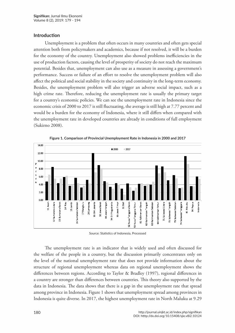
Figure 1. Comparison of Provincial Unemployment Rate in Indonesia in 2000 and 2017

Source: Statistics of Indonesia, Processed

The unemployment rate is an indicator that is widely used and often discussed for the welfare of the people in a country, but the discussion primarily concentrates only on the level of the national unemployment rate that does not provide information about the structure of regional unemployment whereas data on regional unemployment shows the differences between regions. According to Taylor & Bradley (1997), regional differences in a country are stronger than differences between countries. This theory also supported by the data in Indonesia. The data shows that there is a gap in the unemployment rate that spread among province in Indonesia. Figure 1 shows that unemployment spread among provinces in Indonesia is quite diverse. In 2017, the highest unemployment rate in North Maluku at 9.29

181

Eka Khaerandy OktafiantoDeterminant of Regional Unemployment

http://journal.uinjkt.ac.id/index.php/signifikanDOI: htttp://dx.doi.org/10.15408/sjie.v8i2.10124

percent and the lowest in Bali at 1.48 percent. Besides that, in 2017 there are ten provinces that have unemployment rates above the national average. This condition is not too much different in 2000. From the data in Figure 1, it shows that from 2000-2017, there were still problems regarding unemployment in Indonesia.

Elhorst (2003) mentioned at least three main reasons why it is necessary to analyze unemployment at the regional level. First, there is a gap in the regional unemployment rate. This fact is indicating the performance of the labor market at the regional level and referring to problems that exist at the regional level. So, it is essential for governments at the regional level must deal with the regional labor market more seriously. Second, most macroeconomic studies try to explain the unemployment gap between countries and conclude that differences in labor market institutions are the primary source of uneven distribution. However, in a country, such institutions are general and cannot be used as explanations. Existing theories about regional unemployment show that other factors must compensate for high unemployment in some regions. Therefore, it is essential to identify variables that can explain regional differences that exist in the long-run balance. Third, the regional unemployment gap has the potential to cause inefficiencies. Therefore, if it is successfully resolved, this is likely to provide substantial benefits such as higher national output and a decrease in inflation pressure (Taylor & Bradley, 1997).

The problem of unemployment also can not be separated from the labor market. One characteristic of the regional labor market is it related to the regional dimension. The existence of spatial dependencies shows that the regional unemployment rate in a particular region will be related to the neighboring region (neighboring effect). The existence of spatial dependencies can cause by economic activities of a region that affect resources in another adjacent region. For example, if there is an employment opening in a new area, it will absorb labor not only in the region but also in the neighboring region. Thus this will reduce unemployment in both regions. This phenomenon happens because companies/employers do not limit their recruitment activities to the location of their residents but also the surrounding area. This fact is why there is spatial econometrics, which states that ignoring this spatial effect will lead to biased and inefficient estimates (Anselin and Bera, 1998). However, due to the existence of spatial dependencies, the errors between observations will be correlated so that the assumption of non-autocorrelation will violate. As a result, the estimated parameters are still unbiassed and consistent, but the variance will be significant (inefficient), so the estimator is no longer the best linear unbiased estimator (BLUE). Therefore, in this study, we applied spatial econometrics to avoid this deficiency.

Many researchers have researched regional unemployment. From a methodological view, empirical literature can divide into several things. First, the model for regional unemployment is estimated using panel data (non-spatial) techniques. An example is research conducted by Kiral and Mavruk (2017), which aims to investigate the unemployment gap and its relationship with the labor market in Turkey. Besides that, Soekarni et al. (2009) that examine the persistence of unemployment rates in Indonesia, then identify the factors that cause regional unemployment rates at some point in the area. Second, the regional unemployment model uses spatial econometrics by using cross-section data. Some of them are



research conducted by Filiztekin (2008) examining the spatial pattern of unemployment in Turkey and the factors that influence regional unemployment. Third, regional unemployment models use spatial econometrics using panel data. Some of them are research conducted by Guclu (2017) which also uses the method of spatial error (SEM) and spatial lag models (SAR) to analyze the phenomenon of the gap in unemployment rates between regions in Turkey as well as knowing its spillover effect. Ilahi et al. (2014) also use the method of spatial lag (SAR) to analyze the unemployment rate in the Province of Bangka Belitung using panel data from 2008-2013. This data proves that spatial interactions concerning unemployment in a region cannot be separated.

Therefore, this study gives a contribution by applying the third method above to determine the factors that affect the regional unemployment in Indonesia by using spatial aspect to avoid bias that could be caused by their spatial dependence because it is only a few studies that had to analyze the phenomenon of unemployment from the perspective of the spatial and regional dimension in Indonesia. Besides that, analyzing from a geographical view is also essential to be carried out to identify whether there are similarities in the characteristics of neighboring regions and to see the spatial concentration of the unemployment rate.

The purposes of this research are: first, identifying the general information about the level of unemployment in Indonesia. Second, identifying the determinants of the unemployment rate in Indonesia. Third, calculating the direct, indirect, and total effects of the independent variables are used to the variable unemployment rate in Indonesia. All are from 2000 to 2017.

Method he data used in this study are secondary panel data with a span of 18 years, starting

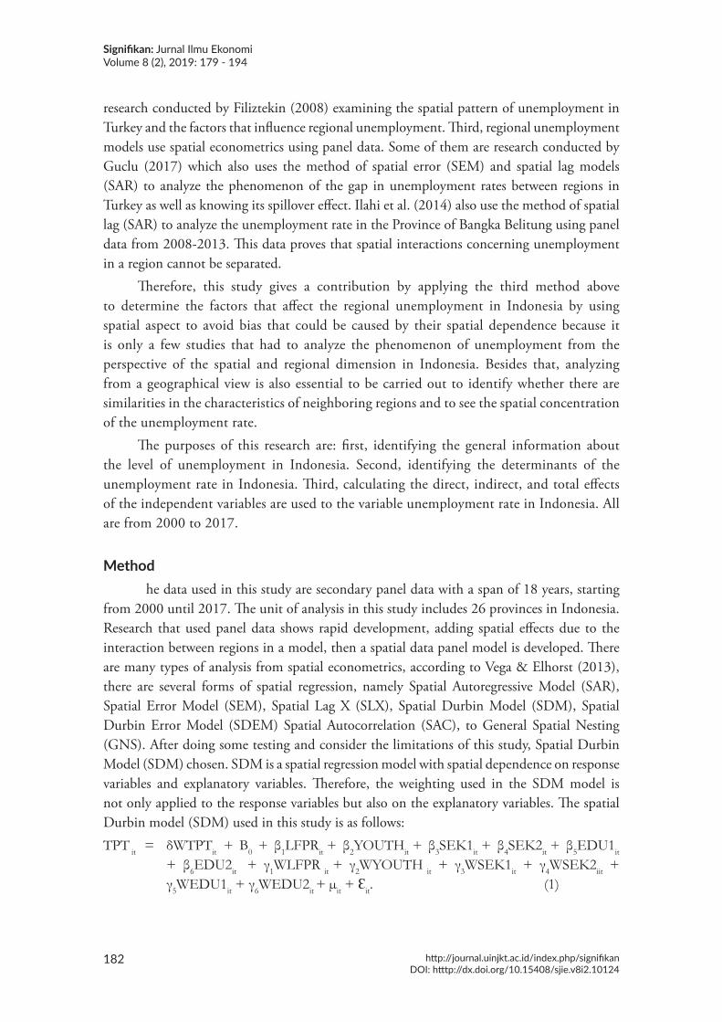
from 2000 until 2017. The unit of analysis in this study includes 26 provinces in Indonesia. Research that used panel data shows rapid development, adding spatial effects due to the interaction between regions in a model, then a spatial data panel model is developed. There are many types of analysis from spatial econometrics, according to Vega & Elhorst (2013), there are several forms of spatial regression, namely Spatial Autoregressive Model (SAR), Spatial Error Model (SEM), Spatial Lag X (SLX), Spatial Durbin Model (SDM), Spatial Durbin Error Model (SDEM) Spatial Autocorrelation (SAC), to General Spatial Nesting (GNS). After doing some testing and consider the limitations of this study, Spatial Durbin Model (SDM) chosen. SDM is a spatial regression model with spatial dependence on response variables and explanatory variables. Therefore, the weighting used in the SDM model is not only applied to the response variables but also on the explanatory variables. The spatial Durbin model (SDM) used in this study is as follows:TPT it = δWTPTit +Β0 + β1LFPRit + β2YOUTHit + β3SEK1it + β4SEK2it + β5EDU1it

+ β6EDU2it + γ1WLFPR it + γ2WYOUTH it + γ3WSEK1it + γ4WSEK2iit + γ5WEDU1it+γ6WEDU2it + µit + Ɛit. (1)

183



Where: TPT is the Unemployment rate (percent); LFPR is the Labor force participation rate (percent); YOUTH is The proportion of young people (15-24) to the working-age population (15-64); EDU1 is People who have a higher education level (natural logarithm); EDU2 is People who have the education level of high school or vocational school and lower (natural logarithm); SEK1 is Share of workers in the manufacturing sector to total workers (percent); SEK2 is Share of workers in the service sector to total workers (percent).

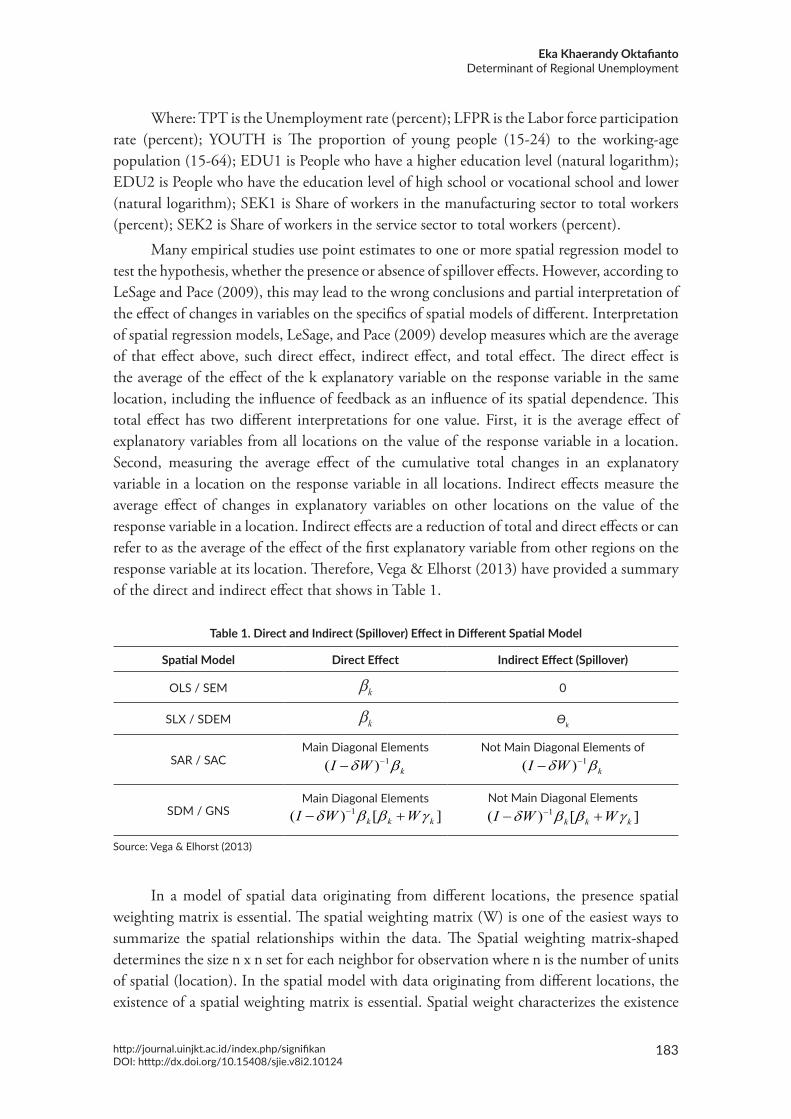
Many empirical studies use point estimates to one or more spatial regression model to test the hypothesis, whether the presence or absence of spillover effects. However, according to LeSage and Pace (2009), this may lead to the wrong conclusions and partial interpretation of the effect of changes in variables on the specifics of spatial models of different. Interpretation of spatial regression models, LeSage, and Pace (2009) develop measures which are the average of that effect above, such direct effect, indirect effect, and total effect. The direct effect is the average of the effect of the k explanatory variable on the response variable in the same location, including the influence of feedback as an influence of its spatial dependence. This total effect has two different interpretations for one value. First, it is the average effect of explanatory variables from all locations on the value of the response variable in a location. Second, measuring the average effect of the cumulative total changes in an explanatory variable in a location on the response variable in all locations. Indirect effects measure the average effect of changes in explanatory variables on other locations on the value of the response variable in a location. Indirect effects are a reduction of total and direct effects or can refer to as the average of the effect of the first explanatory variable from other regions on the response variable at its location. Therefore, Vega & Elhorst (2013) have provided a summary of the direct and indirect effect that shows in Table 1.

Table 1. Direct and Indirect (Spillover) Effect in Different Spatial Model

Spatial Model Direct Effect Indirect Effect (Spillover)

OLS / SEM 0

SLX / SDEM Өk

SAR / SACMain Diagonal Elements

1( ) kI Wδ β−−Not Main Diagonal Elements of

1( ) kI Wδ β−−

SDM / GNSMain Diagonal Elements

1( ) [ ]k k kI W Wδ β β γ−− +Not Main Diagonal Elements

1( ) [ ]k k kI W Wδ β β γ−− +

Source: Vega & Elhorst (2013)

In a model of spatial data originating from different locations, the presence spatial weighting matrix is essential. The spatial weighting matrix (W) is one of the easiest ways to summarize the spatial relationships within the data. The Spatial weighting matrix-shaped determines the size n x n set for each neighbor for observation where n is the number of units of spatial (location). In the spatial model with data originating from different locations, the existence of a spatial weighting matrix is essential. Spatial weight characterizes the existence



of inter-location dependence (spatial dependence) so that the spatial weight measure has an essential influence on the estimation of the spatial dependence model. The weighting matrix to be used in this study is the inverse distance.

Inverse distance method is determined based on the actual distance between locations. The inverse distance matrix gives a substantial weight value for closer distances and smaller weights for longer distances. Calculation of distance between locations can use latitude and longitude coordinates from the observed center point of location. For ease of interpretation, normalization of the W matrix is done so that the number of weighting elements from each row becomes one. Because W is a non-negative matrix, this makes all the weights between each spatial unit worth between 0 and 1.

The global moran index is used to identify and recognize the existence of spatial autocorrelation in response variables (Arifatin, 2018). Spatial autocorrelation is an estimate of the observed value related to the spatial location of the same variable. Positive autocorrelation shows the similarity of values from adjacent locations and tends to group. Spatial autocorrelation can also show from the moran index coefficient. The zero moran index value indicates no spatial autocorrelation; the positive moran index value indicates positive spatial autocorrelation which means that adjacent locations have similar values and are (high-high) or (low-low), and negative moran index value indicates negative spatial autocorrelation which means that adjacent locations have different values.

Results and DiscussionOverview The Unemployment Rate In Indonesia

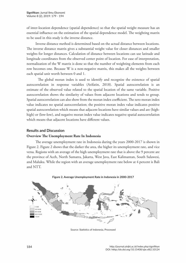
The average unemployment rate in Indonesia during the years 2000-2017 is shown in Figure 2. Figure 2 shows that the darker the area, the higher its unemployment rate, and vice versa. Regions with an average of the high unemployment rate that is above the 9 percent are the province of Aceh, North Sumatra, Jakarta, West Java, East Kalimantan, South Sulawesi, and Maluku. While the region with an average unemployment rate below at 4 percent is Bali and NTT.

Figure 2. Average Unemployment Rate in Indonesia in 2000-2017


185



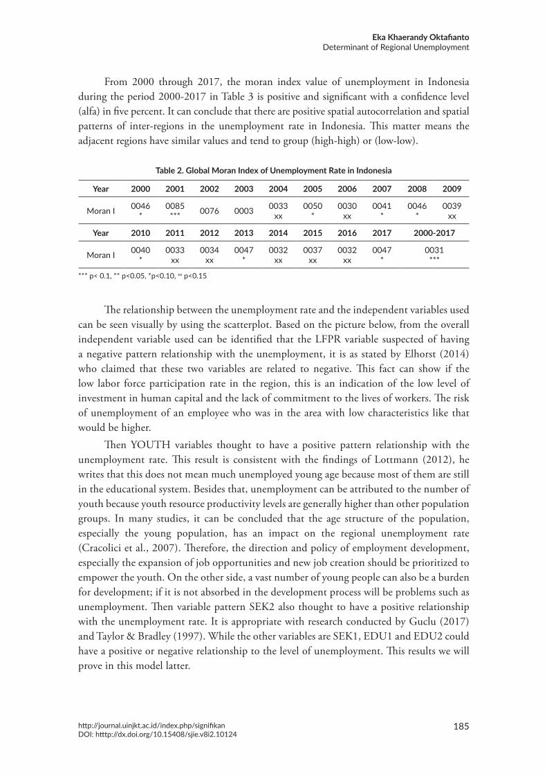
From 2000 through 2017, the moran index value of unemployment in Indonesia during the period 2000-2017 in Table 3 is positive and significant with a confidence level (alfa) in five percent. It can conclude that there are positive spatial autocorrelation and spatial patterns of inter-regions in the unemployment rate in Indonesia. This matter means the adjacent regions have similar values and tend to group (high-high) or (low-low).

Table 2. Global Moran Index of Unemployment Rate in Indonesia

Year 2000 2001 2002 2003 2004 2005 2006 2007 2008 2009

Moran I 0046*

0085*** 0076 0003 0033

xx0050

*0030

xx0041

*0046

*0039

xx

Year 2010 2011 2012 2013 2014 2015 2016 2017 2000-2017

Moran I 0040*

0033 xx

0034 xx

0047*

0032 xx

0037 xx

0032 xx

0047*

0031***

*** p< 0.1, ** p<0.05, *p<0.10, xx p<0.15

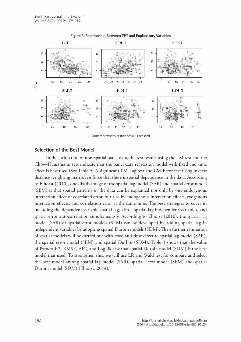
The relationship between the unemployment rate and the independent variables used

can be seen visually by using the scatterplot. Based on the picture below, from the overall independent variable used can be identified that the LFPR variable suspected of having a negative pattern relationship with the unemployment, it is as stated by Elhorst (2014) who claimed that these two variables are related to negative. This fact can show if the low labor force participation rate in the region, this is an indication of the low level of investment in human capital and the lack of commitment to the lives of workers. The risk of unemployment of an employee who was in the area with low characteristics like that would be higher.

Then YOUTH variables thought to have a positive pattern relationship with the unemployment rate. This result is consistent with the findings of Lottmann (2012), he writes that this does not mean much unemployed young age because most of them are still in the educational system. Besides that, unemployment can be attributed to the number of youth because youth resource productivity levels are generally higher than other population groups. In many studies, it can be concluded that the age structure of the population, especially the young population, has an impact on the regional unemployment rate (Cracolici et al., 2007). Therefore, the direction and policy of employment development, especially the expansion of job opportunities and new job creation should be prioritized to empower the youth. On the other side, a vast number of young people can also be a burden for development; if it is not absorbed in the development process will be problems such as unemployment. Then variable pattern SEK2 also thought to have a positive relationship with the unemployment rate. It is appropriate with research conducted by Guclu (2017) and Taylor & Bradley (1997). While the other variables are SEK1, EDU1 and EDU2 could have a positive or negative relationship to the level of unemployment. This results we will prove in this model latter.



Figure 3. Relationship Between TPT and Explanatory Variables


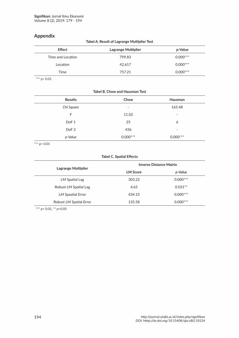
Selection of the Best ModelIn the estimation of non-spatial panel data, the test results using the LM test and the

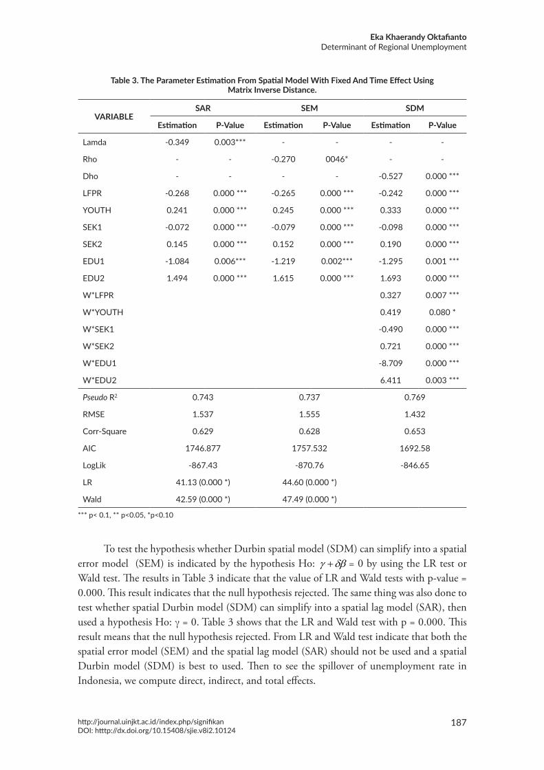
Chow-Haussmann test indicate that the panel data regression model with fixed and time effect is best used (See Table A. A significant LM-Lag test and LM-Error test using inverse distance weighting matrix reinforce that there is spatial dependence in the data. According to Elhorst (2010), one disadvantage of the spatial lag model (SAR) and spatial error model (SEM) is that spatial patterns in the data can be explained not only by one endogenous interaction effect or correlated error, but also by endogenous interaction effects, exogenous interaction effects, and correlation error at the same time. The best strategies to cover it, including the dependent variable spatial lag, also k spatial lag independent variables, and spatial error autocorrelation simultaneously. According to Elhorst (2010), the spatial lag model (SAR) or spatial error models (SEM) can be developed by adding spatial lag in independent variables by adopting spatial Durbin models (SDM). Then further estimation of spatial models will be carried out with fixed and time effect to spatial lag model (SAR), the spatial error model (SEM) and spatial Durbin (SDM). Table 3 shows that the value of Pseudo-R2, RMSE, AIC, and LogLik saw that spatial Durbin model (SDM) is the best model that used. To strengthen this, we will use LR and Wald test for compare and select the best model among spatial lag model (SAR), spatial error model (SEM) and spatial Durbin model (SDM) (Elhorst, 2014).

187



Table 3. The Parameter Estimation From Spatial Model With Fixed And Time Effect Using Matrix Inverse Distance.

VARIABLESAR SEM SDM

Estimation P-Value Estimation P-Value Estimation P-Value

Lamda -0.349 0.003*** - - - -

Rho - - -0.270 0046* - -

Dho - - - - -0.527 0.000 ***

LFPR -0.268 0.000 *** -0.265 0.000 *** -0.242 0.000 ***

YOUTH 0.241 0.000 *** 0.245 0.000 *** 0.333 0.000 ***

SEK1 -0.072 0.000 *** -0.079 0.000 *** -0.098 0.000 ***

SEK2 0.145 0.000 *** 0.152 0.000 *** 0.190 0.000 ***

EDU1 -1.084 0.006*** -1.219 0.002*** -1.295 0.001 ***

EDU2 1.494 0.000 *** 1.615 0.000 *** 1.693 0.000 ***

W*LFPR 0.327 0.007 ***

W*YOUTH 0.419 0.080 *

W*SEK1 -0.490 0.000 ***

W*SEK2 0.721 0.000 ***

W*EDU1 -8.709 0.000 ***

W*EDU2 6.411 0.003 ***

Pseudo R2 0.743 0.737 0.769

RMSE 1.537 1.555 1.432

Corr-Square 0.629 0.628 0.653

AIC 1746.877 1757.532 1692.58

LogLik -867.43 -870.76 -846.65

LR 41.13 (0.000 *) 44.60 (0.000 *)

Wald 42.59 (0.000 *) 47.49 (0.000 *)

*** p< 0.1, ** p<0.05, *p<0.10

To test the hypothesis whether Durbin spatial model (SDM) can simplify into a spatial error model (SEM) is indicated by the hypothesis Ho: γ δβ+ = 0 by using the LR test or Wald test. The results in Table 3 indicate that the value of LR and Wald tests with p-value = 0.000. This result indicates that the null hypothesis rejected. The same thing was also done to test whether spatial Durbin model (SDM) can simplify into a spatial lag model (SAR), then used a hypothesis Ho: γ = 0. Table 3 shows that the LR and Wald test with p = 0.000. This result means that the null hypothesis rejected. From LR and Wald test indicate that both the spatial error model (SEM) and the spatial lag model (SAR) should not be used and a spatial Durbin model (SDM) is best to used. Then to see the spillover of unemployment rate in Indonesia, we compute direct, indirect, and total effects.



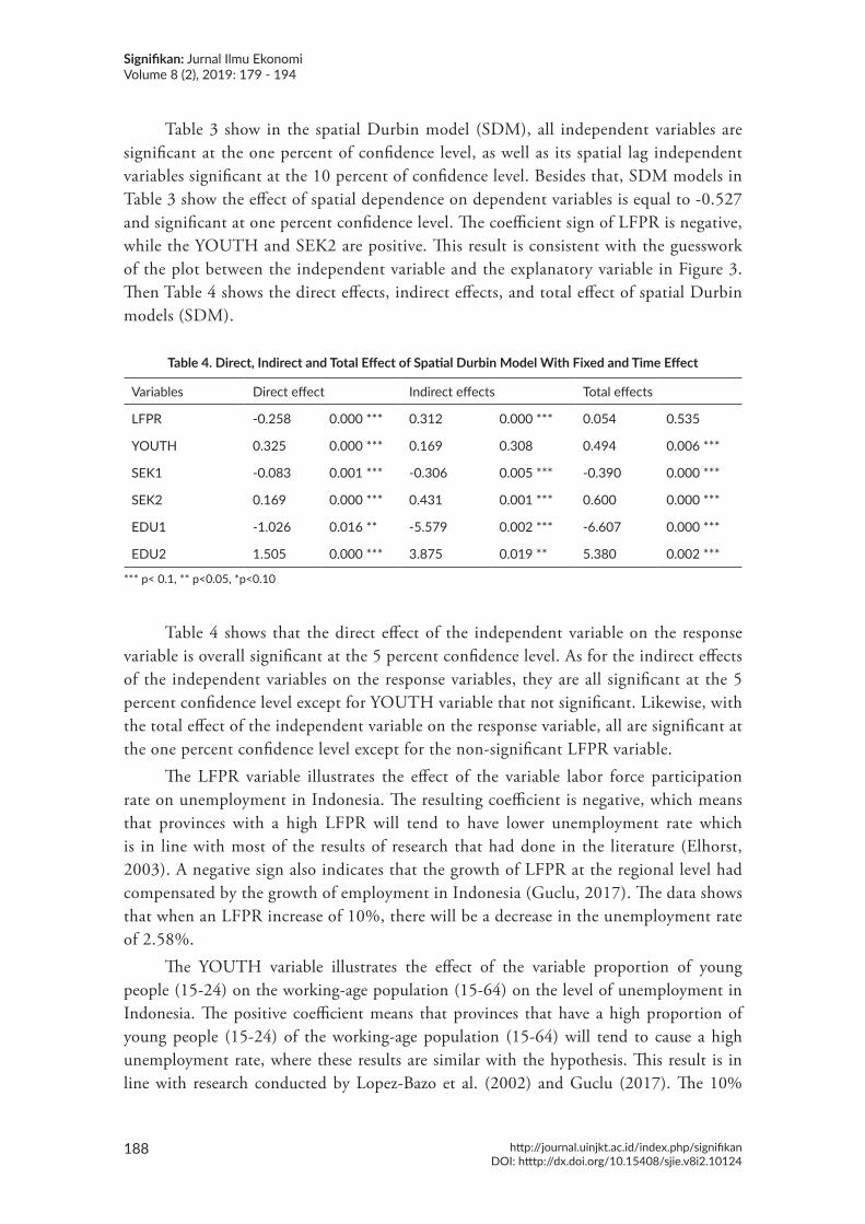
Table 3 show in the spatial Durbin model (SDM), all independent variables are significant at the one percent of confidence level, as well as its spatial lag independent variables significant at the 10 percent of confidence level. Besides that, SDM models in Table 3 show the effect of spatial dependence on dependent variables is equal to -0.527 and significant at one percent confidence level. The coefficient sign of LFPR is negative, while the YOUTH and SEK2 are positive. This result is consistent with the guesswork of the plot between the independent variable and the explanatory variable in Figure 3. Then Table 4 shows the direct effects, indirect effects, and total effect of spatial Durbin models (SDM).

Table 4. Direct, Indirect and Total Effect of Spatial Durbin Model With Fixed and Time Effect

Variables Direct effect Indirect effects Total effects

LFPR -0.258 0.000 *** 0.312 0.000 *** 0.054 0.535

YOUTH 0.325 0.000 *** 0.169 0.308 0.494 0.006 ***

SEK1 -0.083 0.001 *** -0.306 0.005 *** -0.390 0.000 ***

SEK2 0.169 0.000 *** 0.431 0.001 *** 0.600 0.000 ***

EDU1 -1.026 0.016 ** -5.579 0.002 *** -6.607 0.000 ***

EDU2 1.505 0.000 *** 3.875 0.019 ** 5.380 0.002 ***

*** p< 0.1, ** p<0.05, *p<0.10

Table 4 shows that the direct effect of the independent variable on the response variable is overall significant at the 5 percent confidence level. As for the indirect effects of the independent variables on the response variables, they are all significant at the 5 percent confidence level except for YOUTH variable that not significant. Likewise, with the total effect of the independent variable on the response variable, all are significant at the one percent confidence level except for the non-significant LFPR variable.

The LFPR variable illustrates the effect of the variable labor force participation rate on unemployment in Indonesia. The resulting coefficient is negative, which means that provinces with a high LFPR will tend to have lower unemployment rate which is in line with most of the results of research that had done in the literature (Elhorst, 2003). A negative sign also indicates that the growth of LFPR at the regional level had compensated by the growth of employment in Indonesia (Guclu, 2017). The data shows that when an LFPR increase of 10%, there will be a decrease in the unemployment rate of 2.58%.

The YOUTH variable illustrates the effect of the variable proportion of young people (15-24) on the working-age population (15-64) on the level of unemployment in Indonesia. The positive coefficient means that provinces that have a high proportion of young people (15-24) of the working-age population (15-64) will tend to cause a high unemployment rate, where these results are similar with the hypothesis. This result is in line with research conducted by Lopez-Bazo et al. (2002) and Guclu (2017). The 10%

189



increase in the proportion of young people (15-24) to the working-age population (15-64) in a province will increase the unemployment rate in that province about 3.325 percent, and is also associated with an increase in the unemployment rate about 1,69 percent in neighboring provinces, and overall it is related to the increase in unemployment rates in both the region and neighboring regions by 4.94 percent. The regression results affirm that the young population has a positive impact on the regional unemployment rate in Indonesia. This result does not mean that many of the unemployed young people, but they are many who are still in the educational system (Lottmann, 2012). Biagi and Lucifora (2008) find that structural shifts in the population age structure play an essential role in the variation of unemployment rates.

Variable SEK1 illustrates the effect of the share of workers employed in sectors manafaktur in the unemployment rate in Indonesia. The resulting coefficient is negative, which means that the province with the high share of workers employed in sectors manufacture has contributed to the decline in the unemployment rate where it is in line with research conducted by Lottmann (2012), but contrary with the findings of Guclu (2017). The 10% increase in the percentage of workers working in the manufacturing sector in a province will help reduce the unemployment rate in the province by 0.83%, and also reduce unemployment in the neighboring province (spillover effect) by 3.06%, and overall it is related to the decline in the unemployment rate in both the region and neighboring regions by 3.90 percent. It shows that the effect was better on reducing the unemployment rate in neighboring provinces than its provinces.

Variable SEK2 illustrates the effect of the share of workers employed in the service sector to the unemployment rate in Indonesia. Resulting coefficient is positive, which means that the province with the high share of workers employed in the services sector has contributed to an increase in the unemployment rate both on its regions and in neighboring regions, when compared to provinces that have fewer share of workers who work in the service sector, where this is in line with research conducted by Guclu (2017), and Taylor & Bradley (1997). We can say that the 10% increase in the percentage of workers employed in the services sector in the province will help improve the unemployment rate in the province up to 1.69%, and also increase unemployment in the neighboring province (spillover effects) of approximately 4.31%, and also be associated with an increased overall unemployment rate in both the region and the neighboring region of 6.00 percent. It turned out that the effects were worse on the neighboring provinces.

Variables SEK1 and SEK2 called Industrial Mix. It is another determinant of regional unemployment empirically derived. The estimation results show that employment growth in the service sector may be inadequate to compensate for the loss of employment in the manufacturing / industrial sector or in other words: workers who work in the service sector tend to lose their jobs more efficiently compared to the manufacturing / industrial sector. This result is contrary to the increasing trend in the service sector. Therefore, an increase in unemployment is more likely to occur in regions that have specialization in the service sector compared to the manufacturing sector. (Guclu, 2017).



The EDU1 variable describes the influence of population who has a higher education level on the level of unemployment in Indonesia. The resulting coefficients are negative which means that the province with a share of the population that has a higher education level contributes to the decline in the unemployment rate, which this is in line with the research conducted by Guclu (2017) and Flitzekin (2009). This means that a 10% increase in the percentage of population who have a higher education level in a province will cause a decrease in the level of open unemployment in the province by 10.26%, and also reduce unemployment in the neighboring province (spillover effect) around -53.79% and it also turns out that overall it is related to the decline in the unemployment rate in both the region and the neighboring region by 66.07 percent.

Variable EDU2 illustrates the effect of the population that has a secondary education and lowers to the unemployment rate in Indonesia. The resulting coefficient is positive which means that the province with the percentage of the population has a medium level of education has contributed to an increase in the open unemployment rate where it is in line with research conducted by Koze and Gunez (2013). These results indicate that a 10% increase in the population of secondary education level will trigger an increase in the provincial unemployment rate of 15.06% and an increase in the unemployment rate of the neighboring province (spillover effect) of 38.75%.

It can show that higher education is a variable that significantly influences the decline in the unemployment rate in Indonesia. The more regions where citizens have higher levels of education, the better effect will be to reduce unemployment in both the region and the neighboring regions. Research conducted by Eggert et al. also supports this research., (2010), Mondschean & Oppenheimer (2011), Riddell and Song (2011), Kose & Gunez (2013), Guclu (2017), Lavrinovicha et al., (2015), and Snieska et al., (2015). This fact could be due to several things, such as: First, those employment needs are widely available to those who have higher education. Second, those who have higher education will be more independent and easier to creating employment. This result is different from Hall (2016) that concludes no evidence having attended a longer education will reduce the risk of experiencing unemployment.

ConclusionAlthough some studies have tried to identify the underlying causes of unemployment

at the national level in Indonesia, very little work so far had done at the regional level by involving the spatial aspect. In the context of this paper, we try to show that there is some information that could be useful in identifying gaps in regional unemployment in Indonesia. The empirical results reveal that most of the causes of the gap in the unemployment rate can be explained by following the main regional variables: educational attainment (human capital), a young population, industrial mix, and the labor force participation rate. Based on that mean regional variable, higher education that has a big significant impact for reducing regional unemployment so that policymaker should give attention to this. Besides that, policymakers need to implement policies that encourage job creation,

191



especially in the manufacturing sector. The promotion mechanism must be implemented by paying attention not only to under-developed regions but also mainly to areas with high unemployment even though they are not underdeveloped areas such as in Jakarta, West Java or East Kalimantan.

The empirical analysis presents two more essential findings. First, there is spatial dependence between regions. This result means that the increase in the unemployment rate will lead to the growth of the unemployment rate in the neighboring region. Second, spillover effects are detected. It concludes that the factors that influence unemployment in a region not only affect unemployment in the region but also affect unemployment in neighboring regions. Such effects of dependence and spillover can cause polarization of the unemployment rate in the labor market in Indonesia. In other words, this results in a grouping of regions where high (or low) unemployment is experiencing. When going to consider the spillover effect, the government must not ignore the fact that implementing a policy to reduce unemployment in a region will have an impact on reducing unemployment in the neighboring region.

ReferencesAnselin, L., & Bera, A.K. (1998). Spatial Dependence in Linear Models Regression Spatial

With An Introduction to Econometrics. In Ullah, A., & Giles, D. E. A (Eds). Handbook of Applied Economics Statistics, New York: Dekker.

Arifatin, D. (2018). Analisis Spasial Data Panel Untuk Mengkaji Faktor-Faktor yang Mempengaruhi Kunjungan Wisatwan Mancanegara di Indonesia Tahun 2011-2015 (Spatial Analysis of Panel Data to Assess Factors Affecting Foreign Tourist Visits in Indonesia in 2011-2015). Unpublished Thesis. Bogor: Bogor Agricultural University.

Biagi, F., & Lucifora, C. (2008). Demographic and Education Effects on Unemployment in Europe. Labour Economics, 15(5), 1076-1101. https://doi.org/10.1016/j.labeco.2007. 09.006.

Cracolici, M.F., Cuffaro, M., & Njkamp, P. (2007). A Geographical Distribution of Unemployment: An Analysis of Provincial D ifference in Italy. Growth and Change Journal, 38 (4), 649-670. https://doi.org/10.1111/j.1468-2257.2007.00391.x.

Eggert, W., Krieger, T., & Meier, V. (2010). Education, Unemployment, and Migration. Journal of Public Economics, 94(5-6), 354-362. https://doi.org/10.1016/j.jpubeco.2010. 01.005

Elhorst, J.P. (2003). The Mystery of Regional Unemployment Differentials: Theoretical and Empirical Explanation. Journal of Economics Survey, 17(5), 709-748. https://doi.org/10.1046/j.1467-6419.2003.00211.x.

Elhorst, J.P. (2010). Applied Spatial Econometrics: Raising the bar. Spatial Economics Analysis, 5 (1), 9-28. https://doi.org/10.1080/17421770903541772.

Elhorst, J.P. (2014). Spatial Panel Data Models. Handbook of Regional Science. Springer: Berlin pp. 1637-1652.



Filiztekin, A. (2008). Regional Unemployment in Turkey. Papers in Regional Science, 88(4), 863-873. https://doi.org/10.1111/j.1435-5957.2009.00237.x.

Guclu, M. (2017). Regional Unemployment Disparities in Turkey. Romanian Journal for Economic Forecasting, 20(2), 94-108.

Hall, C. (2016). Does More General Education Reduce the Risk of Future Unemployment? Evidence from an Expansion of Vocational Upper Secondary Education. Economics of Education Review, 52, 251-271. https://doi.org/10.1016/j.econedurev.2016.03.005.

Ilahi, R., Shamsuddin, M., & Suparman, M. (2017). Spatial Durbin Model Fix With Unemployment Rate in Effect for Bangka Belitung. Unpublished Thesis. Bandung: University of Padjadjaran.

Kiral, E., & Mavruk, C. (2017). Regional Unemployment Disparities in Turkey. Finans Politics and Economics Yorumlar, 54(634), 107-134.

Kose, S., & Gunes, S. (2013). Regional Disparities and Persistence assesing The Evidence From Greek Regions, 1991-2008. Regional and Sectoral Economics Studies, 12(1), 55-77.

Lavrinovicha, I., Lavrinenko, O., & Teivans-Treinovskis, J. (2015). Influence of Education on Unemployment Rate and Incomes of Residents. Procedia Social and Behavioral Sciences, 174, 3824-3831. https://doi.org/10.1016/j.sbspro.2015.01.1120.

LeSage, J. P, & Pace, R. K. (2009). Introduction to Spatial Econometrics, 1st Edition. New York: Chapman & Hall/CRC.

Lopez-Bazo, E., Barrio, T. D., & Artis, M. (2002). The Regional Distribution of Spanish Unemployment: A Spatial Analysis. Paper in Regional Science, 81 (2), 365-389. https://doi.org/10.1007/s101100200128.

Lottmann, F. (2012). Explaining Regional Differences Unemployment in Germany: A Spatial Panel Data Analysis. Discussion Paper No.26, SFB 649.

Mondschean, T., & Oppenheimer, M. (2011). Regional Long-Term and Short-Term Unemployment and Education in Transition: The Case of Poland. The Journal of Economic Asymmetries, 8(2), 23-48. https://doi.org/10.1016/j.jeca.2011.02.004.

Riddell, W. C., & Song, X. (2011). The Impact of Education on Unemployment Incidence and Re-employment Success: Evidence from the U.S. Labour Market. Labour Economics, 18(4), 453-463. https://doi.org/10.1016/j.labeco.2011.01.003.

Snieska, V., Valodkiene, G., Daunoriene, A., & Draksaite, A. (2015). Education and Unemployment in European Union Economic Cycles. Proecedia Social and Behavioral Scienes, 213, 211-216. https://doi.org/10.1016/j.sbspro.2015.11.428.

Soekarni, M., Sugema, I., & Widodo, P.R. (2009). Strategy on Reducing Unemployment Persistence: A Micro Analysis in Indonesia. Bulletin of Monetary Economics and Banking, 12(2), 161-206. https://doi.org/10.21098/bemp.v12i2.370.

Sukirno, S. (2008). Ekonomi Pembangunan (Development Economics). Jakarta. Erlangga.

193



Taylor, J., & Bradley, S. (1997). Unemployment in Europe: A Comparative Analysis of Regional Disparities in Germany, Italy and UK. Kyklos 50 (2), 221-245. https://doi.org/10.1111/1467-6435.00012.

Vega, S. H., & Elhorst, J. P. (2013). On Spatial Econometric Models, Spillover Effects, and W. 53rd Congress of European Regional Science Association (ERSA): Conference papers, Econstor, 1-28.



AppendixTabel A. Result of Lagrange Multiplier Test

Effect Lagrange Multiplier p-Value

Time and Location 799.83 0.000***

Location 42.617 0.000***

Time 757.21 0.000***

*** p< 0.01

Tabel B. Chow and Hausman Test

Results Chow Hausman

Chi Square - 165.48

F 11.02 -

DoF 1 25 6

DoF 2 436 -

p-Value 0.000*** 0.000***

*** p< 0.01

Tabel C. Spatial Effects

Lagrange MultiplierInverse Distance Matrix

LM Score p-Value

LM Spatial Lag 303.22 0.000***

Robust LM Spatial Lag 4.65 0.031**

LM Spastial Error 434.15 0.000***

Robust LM Spatial Error 135.58 0.000***

*** p< 0.01, ** p<0.05

Documents

The Determinant of Regional Unemployment in Indonesia: …