The Cyclical Behavior of the Price-Cost Markupeconweb.ucsd.edu/~vramey/research/markupcyc-long.pdf · · 2010-10-05The Cyclical Behavior of the Price-Cost Markup Christopher J

The Cyclical Behaviorof the Price-Cost Markup

Christopher J. Nekarda1 Valerie A. Ramey2

1Federal Reserve Board of Governors

2University of California, San Diegoand NBER

The views in this paper are the authors’ and do not necessarily represent the viewsor policies of the Board of Governors of the Federal Reserve System or its staff

Introduction

Background

I Keynesian models from the 1930s through the 1970sassumed sticky wages

I e.g., Keynes (1936), Phelps (1968), Taylor (1980)

I In the early 1980s the focus shifted to models with stickyprices and imperfect competition

I Dunlop-Tarshis-Keynes controversy

I Rotemberg (1982) and many others developed models withsticky prices and imperfect competition

Introduction

Background

I Textbook New Keynesian model assumes sticky prices andflexible wages

I e.g. Goodfriend and King (1997), Woodford (2003)

I Newer versions of the New Keynesian model assume bothsticky prices and sticky wages

I e.g. Erceg, Henderson, Levin (2000), Smets and Wouters(2003, 2007), Christiano, Eichenbaum, and Evans (2005)

I These models are used extensively by central banks

Introduction

Role of Markups in New Keynesian Models

I The price-cost markup is a key part of the transmissionmechanism in the New Keynesian model:

I A positive demand shock leads output and marginal cost toincrease. Because prices cannot adjust immediately, themarkup falls.

I A positive technology shock lowers marginal cost andraises output. Because prices cannot adjust immediately,the markup rises.

I Leading New Keynesian models with sticky prices andsticky wages—such as EHL (2000), CEE (2005), andSmets and Wouters (2003, 2007)—also predictcountercyclical markups in response to demand shocks.

Introduction






Introduction






Introduction






Introduction

Smets-Wouters’ ModelPositive productivity shock

Output Markup

−0.5

0.0

0.5

1.0

0 4 8 12 16−0.5

0.0

0.5

1.0

0 4 8 12 16

Expansionary monetary shockOutput Markup

−0.5

0.0

0.5

1.0

0 4 8 12 16−0.5

0.0

0.5

1.0

0 4 8 12 16

Quarter Quarter

Notes: Effects of expansionary shocks on output and markups.

Introduction

Effect of a Demand Shock

I Neoclassical model

A · FL (L,K ) =WP

For constant A and K , an increase in L must beaccompanied by a fall in W/P

I New Keynesian model

A · FL (L,K ) =MWP

If markupM falls, then both L and W/P can increase

Introduction

Effect of a Demand Shock

I Neoclassical model

A · FL (L,K ) =WP

For constant A and K , an increase in L must beaccompanied by a fall in W/P

I New Keynesian model

A · FL (L,K ) =MWP

If markupM falls, then both L and W/P can increase

Introduction

Standard Measure of the Markup

I If marginal cost of labor is proportional to average cost, theprice-cost markup is inversely proportional to labor share

I The New Keynesian Phillips curve literature (e.g.Galí-Gertler, 1999; Sbordone, 2002) argue that inverselabor share is a good approximation to the markup

I Thus, if markups are countercyclical, labor share must beprocyclical

I Is it?

Introduction

Labor Share in Private Business

46

48

50

52

54

56

1950 1955 1960 1965 1970 1975 1980 1985 1990 1995 2000 2005 2010

Percent

Notes: Labor share is wage and salary disbursements divided by income without capital consumption adjustment.Shaded areas indicate NBER-dated recessions; latest recession assumed to have ended in 2009:Q3.

Introduction

I If labor share is countercyclical, how can markups also becountercyclical?

I After showing that the labor share is countercyclical,Rotemberg and Woodford (1999) discuss at length whyMC might be more procyclical than AC

I MC may be more procyclical than AC in the presence of:I Hourly wages that increase with average hours per worker

I Adjustment costs

I Lower elasticity of substitution between L and K(i.e., non-Cobb-Douglas production function)

I Increasing returns to scale

Introduction

What This Paper Does

1. Re-evaluate cyclicality of markups based on average costfor several broad aggregates

2. Construct factors to adjust average costs to properlycapture marginal cost

3. Assess cyclicality of aggregate markups based onmarginal cost, both unconditionally and in response to amonetary policy shock

4. Study response of markup to government spending shocksin 4-digit manufacturing data

Introduction

Findings

1. Markups are procyclical or acyclicalI In both aggregate and industry data, for several measures

of the business cycle

2. Aggregate evidenceI Markups trough during recessions and peak in the middle

of expansions

I Markups are procyclical in response to monetary shocks

3. Detailed industry evidenceI Markups are acyclical in response to government

spending–induced increases in shipments

Theoretical Framework

Outline


Estimating the Marginal-Average Wage Adjustment

The Cyclical Behavior of Markups

Effect of a Monetary Policy Shock on Markups

Discussion of the Aggregate Results

Industry Analysis


Theoretical Markup

(1) M =P

MC

Key points for measuring marginal cost, MC:

I A cost-minimizing firm should equalize the marginal cost ofraising output across all possible margins

I Inputs with adjustment costs have more complicatedmarginal cost structures

I We focus on average hours per worker, which evidencesuggests has negligible adjustment costs


Cost Minimization

I Firms choose average hours per worker, h, to minimize

(2) Cost = WA(h) · hN + (terms not involving h)

subject to Y = F (A · hN, . . .).

I WA(h) is the average hourly wageI N is the number of workersI Y is gross outputI A is the level of labor-augmenting technology


Average Wage

I Bils (1987) argued that WA may be increasing in hbecause of the additional cost of overtime hours

I We specify the average wage as

(3) WS

[1 + ρθ

(vh

)]= λF1(A · hN, . . .)A

I WS is the straight-time wageI ρ is the premium for overtime hoursI θ is the fraction of overtime hours that command a premiumI v is average overtime hours per worker

I The last term captures the idea that firms may have to paya premium for hours worked beyond a 40-hour workweek


Average Wage

I Bils (1987) argued that WA may be increasing in hbecause of the additional cost of overtime hours

I We specify the average wage as

(3) WS

[1 + ρθ

(vh

)]= λF1(A · hN, . . .)A

I WS is the straight-time wageI ρ is the premium for overtime hoursI θ is the fraction of overtime hours that command a premiumI v is average overtime hours per worker

I The last term captures the idea that firms may have to paya premium for hours worked beyond a 40-hour workweek


First-Order Condition for h

I The first-order condition for h is

(4) WS

[1 + ρθ

(dvdh

)]= λF1(A · hN, . . .)A

I λ is the Lagrange multiplier on the constraint (= MC)

I dv/dh is the marginal change in overtime hours for amarginal change in average hours

I F1 is the derivative of F () w.r.t. effective labor, A · hN


Marginal Cost

I Marginal cost of increasing output is

(5) MC = λ =WS

[1 + ρθ

(dvdh

)]AF1(A · hN, . . .)


I F1 is the derivative of F ( ) w.r.t. effective labor, A · hN

I The denominator is marginal product of increasing h

I The numerator is marginal cost of increasing hI Equal to marginal cost of increasing output via N or K


Marginal Cost


(5) MC = λ =WS

[1 + ρθ

(dvdh

)]AF1(A · hN, . . .)






Marginal Cost


(5) MC = λ =WS

[1 + ρθ

(dvdh

)]AF1(A · hN, . . .)






Linking Average Wage and Marginal Wage

I The true marginal cost of raising h is

(6) WM = WS

[1 + ρθ

(dvdh

)]

I Relationship between average wage and marginal wage is

(7)WM

WA=

1 + ρθ(

dvdh

)1 + ρθ

( vh)


Linking Average Wage and Marginal Wage

I The true marginal cost of raising h is

(6) WM = WS

[1 + ρθ

(dvdh

)]

I Relationship between average wage and marginal wage is

(7)WM

WA=

1 + ρθ(

dvdh

)1 + ρθ

( vh)


Measuring Markups (Cobb-Douglas)

I Markup using average wages:

(10) MA =P

WA/ [α (Y/hN)]=α

s

I Markup using marginal wages:

(11) MM =P

WM/ [α (Y/hN)]=

α

s (WM/WA)

I s = (WAhN)/PY is the labor share


Outline






Industry Analysis



(7)WM

WA=

1 + ρθ(

dvdh

)1 + ρθ

( vh)

To construct the ratio of marginal to average wages we require

1. Ratio of overtime hours to average hours2. Marginal change in overtime hours with respect to change

in average hours3. Fraction of overtime hours that command a premium4. Premium paid for overtime hours

Estimating the Marginal-Average Wage Adjustment Measuring v/h


(7)WM

WA=

1 + ρθ(

dvdh

)1 + ρθ

( vh)





Measuring v/h

I There are readily available data on workweek and overtimehours for manufacturing (CES)

I Even at its post-WWII peak, manufacturing accounted foronly a third of employment; it now accounts for less than10 percent of employment

I We construct new series on average hours and overtimehours for the entire economy using a previouslyunderutilized data source


Measuring v/h

I The BLS Employment and Earnings publication providesmonthly data on the number and average hours of personsat work (Cociuba, Prescott, and Ueberfeldt, 2009)

I Employment and Earnings also reports the number ofpersons at work by hours worked

I Hours worked reported in ranges (e.g., 35–39, 40, 41–48)I We use data from the March CPS to calculate the average

of actual hours worked for each published rangeI This yields an approximation of the full distribution of hours

worked, not just the mean

I We consider any hours worked over 40 hours per week tobe “overtime” hours—they need not be paid a premium


Measuring v/h

I We also use monthly CPS data to create household-basedhours for all employees in manufacturing in order tocompare to the establishment-based series for productionworkers.

I Again, we consider any hours worked over 40 hours perweek to be “overtime” hours.


Fig. 1. Average Weekly Hours per Worker, All Workers

37

38

39

40

41

42

1960 1965 1970 1975 1980 1985 1990 1995 2000 2005 2010

Average Weekly Hours per Worker

Notes: Shaded areas indicate NBER-dated recessions.



2

3

4

5

1960 1965 1970 1975 1980 1985 1990 1995 2000 2005 2010

Average Weekly Overtime Hours per Worker




4

6

8

10

12

1960 1965 1970 1975 1980 1985 1990 1995 2000 2005 2010

PublishedEstimated from LPD

Percent of Overtime Hours



Fig. 2. Average Weekly Hours per Worker, Manufacturing

37

38

39

40

41

42

1960 1965 1970 1975 1980 1985 1990 1995 2000 2005 2010

Average Weekly Hours per Worker




2

3

4

5

1960 1965 1970 1975 1980 1985 1990 1995 2000 2005 2010

Average Weekly Overtime Hours per Worker




4

6

8

10

12

1960 1965 1970 1975 1980 1985 1990 1995 2000 2005 2010

PublishedEstimated from LPD

Percent of Overtime Hours


Estimating the Marginal-Average Wage Adjustment Estimating dv/dh


(7)WM

WA=

1 + ρθ(

dvdh

)1 + ρθ

( vh)





Estimating dv/dh

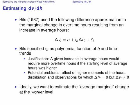
I Bils (1987) used the following difference approximation tothe marginal change in overtime hours resulting from anincrease in average hours:

∆vt = α + ηt ∆ht + ξt

I Bils specified ηt as polynomial function of h and timetrends

I Justification: A given increase in average hours wouldrequire more overtime hours if the starting level of averagehours was higher

I Potential problems: effect of higher moments of the hoursdistribution and observations for which ∆ht = 0 but ∆vt 6= 0

I Ideally, we want to estimate the “average marginal” changeat the worker level


Estimating dv/dh

I We use individual-level data from Nekarda’s (2009)Longitudinal Population Database, a monthly panel dataset constructed from CPS microdata that matchesindividuals across all months, available for 1976 to 2007

I For each matched individual i who is employed in twoconsecutive months we calculate(

∆v∆h

)it

=vit − vi(t−1)

hit − hi(t−1)

I For each month t we take the average over all individuals:

(∆v∆h

)t

=1Pt

Pt∑i=1

(∆v∆h

)it


Estimating dv/dh

I We found that variables from our aggregate EE dataexplained 90 percent of the variation of the estimatedaverage (∆v/∆h)t over 1976 to 2007

I For all civilian workers, the key variables were averagehours of civilian workers and the fraction of workersworking 30 to 40 hours per week

I For manufacturing workers, the key variables were averagehours of production workers in manufacturing and thefraction of all civilian workers who were employed 15–39hours, exactly 40 hours, and 41 hours and more

I We used these fitted values from the regression to projectthe dv/dh series over 1960 to 2009


Fig. 3. Estimated dv/dh

0.20

0.24

0.28

0.32

0.36

0.40

1960 1965 1970 1975 1980 1985 1990 1995 2000 2005 2010

EstimatedProjection

Aggregate Economy



Fig. 3. Estimated dv/dh

0.20

0.24

0.28

0.32

0.36

0.40

1960 1965 1970 1975 1980 1985 1990 1995 2000 2005 2010

EstimatedProjection

Manufacturing


Estimating the Marginal-Average Wage Adjustment Estimating θ


(7)WM

WA=

1 + ρθ(

dvdh

)1 + ρθ

( vh)




Estimating the Marginal-Average Wage Adjustment Estimating θ

Fig. 4. Fraction of Overtime Hours Paid a Premium

24

26

28

30

32

34

36

1970 1975 1980 1985 1990 1995 2000 2005 2010

CPS May extractECEC

Notes: The implied θ for the early sample is based on individual worker reports of hours worked and whether they arepaid a premium from the May CPS extract. The implied θ for the later sample is based on aggregated data on wagesand salaries and overtime compensation from the Employer Cost survey, coupled with our constructed measure ofv/h.

Estimating the Marginal-Average Wage Adjustment Value of ρ


(7)WM

WA=

1 + ρθ(

dvdh

)1 + ρθ

( vh)




Estimating the Marginal-Average Wage Adjustment Value of ρ

Value of ρ

I Statutory overtime premium is 50% for covered employees

I Trejo (1991), Hamermesh (2006): effective rate is around25%

I CES overtime hours for manufacturing are defined asthose that command a premium

I Our aggregate economy hours are simply hours workedabove 40 hours

Estimating the Marginal-Average Wage Adjustment Marginal-Average Wage Adjustment Factor


(7)WM

WA=

1 + ρθ(

dvdh

)1 + ρθ

( vh)





Fig. 5. Marginal-Average Wage Adjustment Factor

1.00

1.01

1.02

1.03

1.04

1960 1965 1970 1975 1980 1985 1990 1995 2000 2005 2010

25 percent (proj.) 50 percent (proj.)25 percent (est.) 50 percent (est.)

Aggregate Economy

Notes: Adjustment factor isWMWA

t =1+ρ( dv/ dh)t

1+ρ(v/h)t. Shaded areas indicate NBER-dated recessions.


Fig. 5. Marginal-Average Wage Adjustment Factor

1.00

1.05

1.10

1.15

1960 1965 1970 1975 1980 1985 1990 1995 2000 2005 2010

25 percent (proj.) 50 percent (proj.)25 percent (est.) 50 percent (est.)

Manufacturing

Notes: Adjustment factor isWMWA

t =1+ρ( dv/ dh)t

1+ρ(v/h)t. Shaded areas indicate NBER-dated recessions.


Outline






Industry Analysis

The Cyclical Behavior of Markups The Markup Measured with Average Wages

Fig. 6. Aggregate Price-Cost Markup

90

100

110

120

1950 1955 1960 1965 1970 1975 1980 1985 1990 1995 2000 2005 2010

Private business (NIPA)Private business (BLS)Manufacturing (NIPA)Nonfinancial corporate business (NIPA)

Index (1997=100)

Notes: Markup in nonfinancial corporate business is compensation divided by gross value added less taxes onproduction; other NIPA markups are wage and salary disbursements divided by income without capital consumptionadjustment. BLS markup is inverse of index of labor share. Shaded areas indicate NBER-dated recessions.

The Cyclical Behavior of Markups The Markup Measured with Average Wages

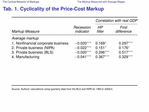
Tab. 1. Cyclicality of the Price-Cost Markup

Correlation with real GDP

Recession HP FirstMarkup Measure indicator filter difference

Average markup1. Nonfinancial corporate business −0.020∗∗∗ 0.169∗ 0.297∗∗∗

2. Private business (NIPA) −0.022∗∗∗ 0.151∗ 0.176∗

3. Private business (BLS) −0.020∗∗∗ 0.296∗∗∗ 0.517∗∗∗

4. Manufacturing −0.041∗∗∗ 0.367∗∗∗ 0.329∗∗∗

Source: Authors’ calculations using quarterly data from the BLS and NIPA for 1960:2–2009:4.

The Cyclical Behavior of Markups The Markup Measured with Marginal Wages

Fig. 7. Marginal Price-Cost Markup, Aggregate Economy

1.7

1.8

1.9

2.0

2.1

1960 1965 1970 1975 1980 1985 1990 1995 2000 2005 2010

Unadjusted50 percent25 percent

Level

Notes: Unadjusted plots average markup in private business sector; remaining series are marginal markup withindicated overtime premium. Cyclical component extracted using HP filter (λ = 1, 600). Shaded areas indicateNBER-dated recessions.


Fig. 7. Marginal Price-Cost Markup, Aggregate Economy

−0.4

−0.2

0.0

0.2

0.4

1960 1965 1970 1975 1980 1985 1990 1995 2000 2005 2010


Cyclical Component

Notes: Unadjusted plots average markup in private business sector; remaining series are marginal markup withindicated overtime premium. Cyclical component extracted using HP filter (λ = 1, 600). Shaded areas indicateNBER-dated recessions.


Fig. 9. Marginal Price-Cost Markup, Manufacturing

1.2

1.4

1.6

1.8

2.0

1960 1965 1970 1975 1980 1985 1990 1995 2000 2005 2010


Level

Notes: Unadjusted plots average markup in manufacturing sector; remaining series are marginal markup with in-dicated overtime premium. Cyclical component extracted using HP filter (λ = 1, 600). Shaded areas indicateNBER-dated recessions.


Fig. 9. Marginal Price-Cost Markup, Manufacturing

−0.8

−0.4

0.0

0.4

0.8

1960 1965 1970 1975 1980 1985 1990 1995 2000 2005 2010


Cyclical Component

Notes: Unadjusted plots average markup in manufacturing sector; remaining series are marginal markup with in-dicated overtime premium. Cyclical component extracted using HP filter (λ = 1, 600). Shaded areas indicateNBER-dated recessions.


Tab. 1. Cyclicality of the Price-Cost Markup

Correlation with real GDP

Recession HP FirstMarkup Measure indicator filter difference

1. Nonfinancial corporate business −0.020∗∗∗ 0.169∗ 0.297∗∗∗

2. Private business (NIPA) −0.022∗∗∗ 0.151∗ 0.176∗

3. Private business (BLS) −0.020∗∗∗ 0.296∗∗∗ 0.517∗∗∗

4. Manufacturing −0.041∗∗∗ 0.367∗∗∗ 0.329∗∗∗

Marginal Markup5. Private business, ρ = 0.25 −0.021∗∗∗ 0.137∗ 0.170∗∗

6. Private business, ρ = 0.50 −0.020∗∗∗ 0.109 0.157∗∗

7. Manufacturing, ρ = 0.25 −0.041∗∗∗ 0.342∗∗∗ 0.322∗∗∗

8. Manufacturing, ρ = 0.50 −0.035∗∗∗ 0.252∗∗∗ 0.272∗∗∗

Source: Authors’ calculations using quarterly data from the BLS and NIPA for 1960:2–2009:4.Notes: Marginal markup for private business uses NIPA measure of labor share.


Fig. 8. Cross-Correlations of Markups with Real GDP

−1.0

−0.8

−0.6

−0.4

−0.2

0.0

0.2

0.4

0.6

0.8

1.0

−8 −6 −4 −2 0 2 4 6 8


Aggregate Economy

−1.0

−0.8

−0.6

−0.4

−0.2

0.0

0.2

0.4

0.6

0.8

1.0

−8 −6 −4 −2 0 2 4 6 8


Manufacturing

Value of j Value of j

Notes: Correlation of cyclical components of yt and µt+j . Detrended using HP filter (λ = 1, 600). Unadjusted isaverage markup in private business sector; remaining series are marginal markup with indicated overtime premium.


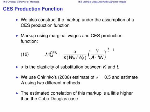
CES Production Function

I We also construct the markup under the assumption of aCES production function

I Markup using marginal wages and CES productionfunction:

(12) MCESM =

α

s (WM/WA)

(Y

A · hN

) 1σ

−1

I σ is the elasticity of substitution between K and L

I We use Chirinko’s (2008) estimate of σ = 0.5 and estimateA using two different methods

I The estimated correlation of this markup is a little higherthan the Cobb-Douglas case


Outline






Industry Analysis


Implications of Procyclical Markups for NK Models

I The New Keynesian (NK) model predicts markup movesprocyclically in response to a technology shock, butcountercyclically in response to a demand shock

I Our finding of procyclical markups may be consistent withthe NK model if technology shocks are the main source ofcyclical fluctuations

I Therefore, we assess the cyclicality of the markupconditional on a demand shock



I We estimate a standard VAR on quarterly data from1960:Q3–2009:Q4

I Variables: log real GDP, log commodity prices, log GDPdeflator, log markup, federal funds rate

I A shock to the federal funds rate (ordered last) is thecontractionary monetary policy shock

I We also consider the cost channel: include prime rate inmarginal cost


Fig. 10. Response of Markup to Contractionary MonetaryPolicy Shock

−0.8

−0.6

−0.4

−0.2

0.0

0.2

0 4 8 12 16 20

Average markup

−0.8

−0.6

−0.4

−0.2

0.0

0.2

0 4 8 12 16 20

Marginal markup (25%)

−0.8

−0.6

−0.4

−0.2

0.0

0.2

0 4 8 12 16 20

Marginal markup (50%)

−0.8

−0.6

−0.4

−0.2

0.0

0.2

0 4 8 12 16 20

Marginal markup (25%), w/ interest rate

−0.8

−0.6

−0.4

−0.2

0.0

0.2

0 4 8 12 16 20

Marginal markup (25%), manufacturing

−0.8

−0.6

−0.4

−0.2

0.0

0.2

0 4 8 12 16 20

Marginal markup (50%), manufacturing

Notes: Impulse responses estimated from VAR(4) with log real GDP, log commodity prices, log GDP deflator, markupmeasure, and federal funds rate; also includes a linear time trend. Monetary policy shock identified as shock tofederal funds rate when ordered last. Specification with interest rate includes the prime rate in marginal cost. Dashedlines indicate 95-percent confidence interval.


Outline






Industry Analysis


Relationship to Bils (1987)

I Our marginal markup is an extension of Bils’s novelconceptual framework, but we reach the oppositeconclusion

I The key is the details of implementation

I In particular, our technological innovations were notavailable in the 1980s

I Higher-frequency data and longer sampleI Richer dataI Conditional estimation based on monetary policy shocks

I Time aggregation is especially important


Relationship to Bils (1987)

I Our marginal markup is an extension of Bils’s novelconceptual framework, but we reach the oppositeconclusion

I The key is the details of implementation

I In particular, our technological innovations were notavailable in the 1980s

I Higher-frequency data and longer sampleI Richer dataI Conditional estimation based on monetary policy shocks

I Time aggregation is especially important


Tab. 3. Effect of Time Aggregation on Markup

Correlation of markup with

Frequency Frequency Industrial Totalof dv/ dh of markup Real GDP production hours

2-digit industry data, 1956–83, 50 Percent Premium1. Quarterly Quarterly 0.307 0.140 0.0692. Quarterly Annual 0.200 0.010 −0.0473. Annual Annual −0.004 −0.205 −0.245

2-digit industry data, 1956–2002, 50 Percent Premium4. Annual Annual 0.011 −0.049 −0.084

2-digit industry data, 1956–2002, 25 Percent Premium5. Annual Annual 0.208 0.153 0.003

Notes: Contemporaneous correlation of cyclical components of log markup and cyclical indicator, where cyclicalcomponent is extracted using HP filter. Industrial production and total hours are for manufacturing.


Relation to the New Keynesian Phillips Curve

I New Keynesian Phillips Curve: πt = βEt (πt+1) + κytI Problem: estimates of κ are negative

I Galí-Gertler (1999): use real marginal cost insteadI πt = βEt (πt+1) + λmct

I Estimates of λ are positive, consistent with theory

I The reason mc enters positively but y enters negatively isthat they are negatively correlated in the data

I Note that mct = − lnMtI Thus, the NKPC explains inflation well because the markup

is procyclical!

Industry Analysis

Outline






Industry Analysis

Industry Analysis

Evidence from Disaggregated Manufacturing Industries

I We now examine detailed 4-digit SIC industry data

I AdvantagesI We can determine whether results are from aggregation

I We can construct a highly relevant demand instrumentbased on industry-specific govt demand

I We can construct markups using gross outputI Basu and Fernald (1997) argue value added is not a natural

measure of outputI Indeed, value added makes sense only when markup is unity

Industry Analysis Data and Variable Construction

Data and Variable Construction

We merge information from:

1. NBER-CEcS Manufacturing Industry DatabaseI Annual data on 458 4-digit SIC industries for 1958–2005

I Data on hours, employment, payrolls, shipments, & capital

I We use information from 2-digit CES data from 1958–2002to create marginal-average wage factors

2. BEA benchmark input-output tablesI Can trace direct and indirect shipments to the government

using transactions and requirements matrices

I Available quinquennially

I We use 1963, 1967, 1972, 1977, 1982, 1987, and 1992

Industry Analysis Data and Variable Construction

Industry-Specific Government Demand

I Nekarda and Ramey (2010) use the following governmentdemand instrument:

∆git = θi ·∆ ln Gt ,

I θi is the average share of industry i ’s total nominalshipments that go to the government

I Gt is aggregate real federal purchases from the NIPA

I Since the distribution of government spending acrossindustries may be correlated with industry-specifictechnological change, this instrument excludes thosechanges (after including industry and time fixed effects)

I The first-stage F statistic of industry shipments on thisinstrument is 193

Industry Analysis Empirical Specification and Results

Industry Regression Specification

I We regress the log change in the markup,∆µit = −∆ ln (sit ), on the log change in real grossshipments, ∆ ln Y :

(18) ∆µit = γ0it + γ1∆ ln Yit + εit ,

I Instrument for ∆ ln Yit using ∆git

I Include industry and year fixed effects (γ0it )

I Sample contains 272 4-digit SIC industries from1960–2002 for a total of 12,009 observations

I γ1 describes how the markup responds to ademand-induced change in output


Industry Regression Specification

I We regress the log change in the markup,∆µit = −∆ ln (sit ), on the log change in real grossshipments, ∆ ln Y :

(18) ∆µit = γ0it + γ1∆ ln Yit + εit ,

I Instrument for ∆ ln Yit using ∆git

I Include industry and year fixed effects (γ0it )

I Sample contains 272 4-digit SIC industries from1960–2002 for a total of 12,009 observations

I γ1 describes how the markup responds to ademand-induced change in output


Tab. 4. Regression of Markup on Gross Shipments

Coefficient γ1

Production AllSpecification workers workers

Average 0.005 0.057(0.052) (0.046)

Marginal (ρ = 0.25) 0.018 0.066(0.052) (0.046)

Marginal (ρ = 0.50) 0.022 0.070(0.052) (0.047)

Notes: IV regression of ∆µit = γ0it + γ1∆ ln Yit + εit . ∆ ln Yit is instrumented by ∆git . Sample contains 2724-digit SIC industries from 1960–2002 for a total of 12,009 observations. All regressions include industry and yearfixed effects.

Conclusion

Conclusions

1. We find no evidence that the markup is countercyclical, inbroad aggregates or detailed manufacturing industries

2. Our results are robust to adjustments of average wages tomarginal wages

3. Our results hold unconditionally as well as conditional ondemand shocks

Conclusion

Implications

I More research is needed to see whether the transmissionmechanism of leading New Keynesian models actuallyholds

I Perhaps a return to models with sticky wages and fairlyflexible prices can make the models consistent with thedata

Documents

The Cyclical Behavior of the Price-Cost Markupeconweb.ucsd.edu/~vramey/research/markupcyc-long.pdf · · 2010-10-05The Cyclical Behavior of the Price-Cost Markup Christopher J