Embed Size (px)
Citation preview
The Cyclical Behavior of Net Interest Margins:
Evidence from the United States Banking Sector
Roger Aliaga-Dıaz∗and Marıa Pıa Olivero†
Preliminary version, comments welcome.
July 2005
AbstractThe paper studies the cyclical behavior of net interest margins
(NIMs) in the United States banking sector, using time series quarterlydata for the period 1979-2005. It documents the countercyclicality ofNIMs and offers potential explanations for this behavior.
Even controlling for important changes in banking regulation thattook place in this period, monetary policy certainly plays a role in ex-plaining the countercyclical behavior. Other determinants are interestrate risk and the economy’s financial depth. At the bank-level, banksliquidity, capital holdings and the share of total assets held by big banksalso exert a significant impact on margins over the cycle. These con-clusions are consistent across several alternative definitions used forNIMs and three different business cycle indicators.
Our results provide support to the bank lending channel of mon-etary policy and to the hypothesis that the effects of monetary policyare weaker in more concentrated banking sectors.
JEL Classification: C32, E32, E44, G21
∗North Carolina State University, Raleigh, NC, 27695. [email protected]†LeBow College of Business, Drexel University, 3141 Chestnut Street, Philadelphia,
PA, 19104. [email protected]
1
1 Introduction
Total loans and leases granted by commercial banks in the United States
averaged almost 45% of gross domestic product in 2004 and the first quarter
of 2005. This figure has been steadily increasing over time1. The ratio of
loans to total bank assets has fluctuated around 60% since 1973. Therefore,
financial sector deepening, if any, does not seem to have lowered the impor-
tance of loans in banks’ portfolios. Both facts are indicative of the relevance
of studies focusing on the market for bank credit in the American economy
and particularly, on its macroeconomic impact.
This paper studies the cyclical behavior of net interest margins (NIMs)
in the United States banking industry, using time series quarterly data for
the period 1979-2005. Our results document the countercyclicality of NIMs.
The contemporaneous sample raw correlation between NIMs and alternative
business cycle indicators is significantly negative in our data. This negative
negative relationship is robust to the inclusion of controls related to monetary
policy, default risk and banking regulation, which are suggested to be the
main determinants of this cyclical behavior.
The paper also offers alternative explanations for the observed behavior.
The business cycle measure loses its explanatory power after an expanded set
of controls is included in the regression of NIMs against a business cycle indi-
cator. This set consists of both macroeconomic and bank-level determinants,
and it completely explains the cyclical behavior of NIMs. Interest rate risk,
the economy’s degree of financial deepening, banks liquidity, capital holdings
and the share of total assets held by big banks all exert a significant impact
on margins.
These conclusions are robust to several alternative definitions for the mar-
1The figure was around 10% in 1947, the first year for which we have data. It was 38%
in 1980.
2
gins and the cycle measure.
Our results have interesting policy implications due to their macroeco-
nomic impacts. When markups vary endogenously in response to aggregate
productivity shocks, which have no direct relation to market structure, their
variation becomes an additional channel through which such shocks can affect
economic activity (Rotemberg and Woodford (1995)). With spreads in the
market for credit being countercyclical according to our results, a financial
accelerator seems to be operating in the American economy. Credit becomes
more expensive in bad times; firms may as a result delay investment and
production decisions and the recession may be made even worse. This may
call for stabilization policies to be made more effective in economies where
these spreads are more countercyclical.
The determinants of margins in the banking sector have been theoreti-
cally studied before. Ho and Saunders (1981) and Saunders and Schumacher
(2000) model procyclical spreads in the market for bank credit. Theirs is a
microeconomic model of banks operating as risk averse dealers. The NIM is
composed of two elements: a producer’s surplus or monopoly rent term, and
a risk adjustment term2. Allen (1988) extends the Ho and Saunders (1981)
model by studying a banks portfolio effect on spreads. She looks at how the
cross-price elasticities of demand among various bank products affect that
pure interest spreads. Wong (1997) develops a model with both credit and
interest rate risk to determine optimal bank NIMs.
Other papers study the empirical determinants of NIMs. Angbazo (1997)
studies the relationship between default and interest rate risk and net interest
margins. Demirguc-Kunt and Huizinga (2000) analyze the effect of financial
development and bank performance on profitability and margins. Angelini
and Cetorelli (2003) look at the impact of regulatory reforms, large scale
2The latter is a function of the banks’ coefficient of absolute risk aversion, the volume
of transactions and the variability of interest rates on deposits and loans.
3
consolidation and competitive pressure on the structure of the Italian bank-
ing industry. Demirguc-Kunt, Laeven and Levine (2004)) study the impact
of bank regulations, market structure and institutions on banks’ efficiency
measured by both NIMs and overhead expenditures.
However, to our knowledge the cyclical behavior of NIMs has been previ-
ously analyzed only by Dueker and Thornton (1997). Thus, we believe this
study is an important empirical contribution. Dueker and Thornton’s frame-
work is significantly different from ours. They build a model with switching
costs for customers and risk averse banks that lead to countercyclical markups
in the pricing of bank loans. They find evidence for loan rates exhibiting a
countercyclical spread over the marginal cost of funds for banks3.
The paper is also closely related to the theoretical literature that mod-
els oligopolistic markets and how various types of strategic interaction may
lead to different patterns for prices and markups. In this work, dynamic
general equilibrium models are used to study the cyclicality of price-cost
margins. The reasons for markups being countercyclical there are, among
others, implicitly colluding oligopolies that find collusion more difficult when
their demand is relatively high (Rotemberg and Saloner (1986)), demand
composition effects such that some types of increases in aggregate demand
imply a procyclical elasticity faced by oligopolistic firms (Gali (1994)), and
“deep habit” formation that allows the demand faced by each individual
producer to depend on past consumption levels, and the price elasticity of
demand to be procyclical (Ravn, Schmitt-Grohe and Uribe (2005)).
Last, our work is related to the vast empirical literature developed after
3Angelini and Cetorelli (2003) include the growth rate of GDP among their regressors
and find a negative impact on both price-cost margins and Lerner indexes in Italy. In
their cross-country study of the impact of bank regulations, market structure and institu-
tions, Demirguc-Kunt, Laeven and Levine (2004) find that economic growth is negatively
(although only weakly) associated with NIMs.
4
Rotemberg and Saloner’s first contribution that measures the cyclicality of
markups in goods markets (Domowitz et al. (1986), Lebow (1992), Chevalier
and Scharfstein (1995 and 1996), Galeotti and Schiantarelli (1998), Bloch and
Olive (2001), Campello (2003), among others).
There are of course explanations for the countercyclical behavior of NIMs
alternative to those offered in this paper. These are more difficult to quan-
tify but future work could try to incorporate them. The first relates to the
banks owners’ preference structure. When adjusting interest rates down-
wards during recessions, banks face the trade-off between profits and market
share. As explained in Dueker and Thornton (1997), if firms with market
power have preferences for smoother profit streams, in recessions they may
smooth profits by charging relatively high prices. The second involves issues
of asymmetric information in the lender-borrower relationship. Banks face
adverse selection when they increase their market share during downturns:
they are faced to borrowers with bigger default probabilities. Therefore, they
may need to increase markups over their marginal costs. Third, the “degree
of market power” may be countercyclical in itself. Forbes and Mayne (1989)
present evidence on the procyclicality of the elasticity of the demand for
credit faced by banks. Fourth, Allen (1988) studies a banks portfolio effect
and extends the Ho and Saunders (1981) model. She shows that pure in-
terest spreads can be reduced when considering the cross-price elasticities of
demand among various bank products. Last, costs of collusion may increase
during economic expansions, as in Rotemberg and Saloner (1986).
The paper proceeds as follows. A review of background literature is pre-
sented in Section 2. A reduced form model for margins is discussed in Section
3. Section 4 describes the econometric methodology and the data used. The
results are shown in Section 5. The last section concludes and outlines some
directions for further research. A detailed description of the data and ex-
tended results are provided in the appendices. The results of some robustness
5
checks can be found in Appendix C.
2 Background Literature
The traditional industrial organization approach states that price wars occur
in recessions. Markups are procyclical as a result. For example, in the
customer market model of Phelps and Winter (1970), a firm that lowers its
current price not only sells more to its current customers, but also expands
its customer base. An increase in aggregate demand implies that profits
rely mainly on current sales and that increasing market shares is relatively
unimportant. Therefore, firms raise their prices in periods of high aggregate
demand, and price-cost margins are directly related to the level of economic
activity.
Rotemberg and Saloner (1986) challenge this view on both theoretical and
empirical grounds. They study the response of oligopolies to fluctuations in
the demand for their goods. The strength of their paper is in their model
that can account for firms behaving more competitively in periods of high
demand. They study implicitly colluding oligopolies4, that find this collusion
more difficult when their demand is relatively high. In booms, there is a larger
gain for a particular firm from lowering the price from the profit maximizing
price for the group. The firm can work with a bigger market by doing so.
The punishment for not cooperating is less affected if it is in the future,
when demand returns to its normal level. The authors also examine the
macroeconomic effects of a shift in demand towards the oligopolistic sector.
In a two-sector model where the other sector is competitive and uses the
4James Friedman (1971) first modeled this type of oligopolistic market where price is
the strategic variable, and where firms threat to revert to competitive behavior whenever
a single firm deviates from oligopolistic pricing. This threat induces cooperation by all
firms.
6
oligopolistic sector’s output as an input, the competitive sector’s output also
increases in periods of high demand5.
Theoretically, countercyclical markups also arise in Gali (1994) and Ravn,
Schmitt-Grohe and Uribe (2005).
Gali (1994) models demand composition effects. Both households and
firms purchase the goods produced by an oligopolistic sector, but they have
different elasticities of substitution between various goods. In this model,
some kinds of increases in aggregate demand, those that imply a change
in its composition, may imply countercyclical markups and have additional
expansionary impacts as a result6.
In Ravn, Schmitt-Grohe and Uribe (2005) agents exhibit “deep habit
formation”. They form habits over individual varieties of goods as opposed
to over a composite consumption good. This allows the demand function
faced by each individual producer to depend on past consumption levels,
and the price elasticity of demand to be procyclical7.
Ho and Saunders (1981) and Saunders and Schumacher (2000) model
margins in the market for bank credit. NIMs are procyclical in their frame-
work. Theirs are microeconomic models of banks operating as risk averse
dealers. The NIM there is composed of two elements: a producer’s surplus
or monopoly rent term, and a risk adjustment term. The latter is a function
of the banks’ coefficient of absolute risk aversion, the volume of transactions
and the variability of interest rates on deposits and loans. The larger the size
of transactions, the bigger NIMs are according to their specification. How-
ever, in their empirical estimation they concentrate on the effects on margins
of market structure and volatility. They do not look at the impacts of risk
5Rotemberg and Woodford (1992) also work with the implicit collusion model.6In Gali (1994) the inefficiency wedge is a monotonically decreasing function of the
share of investment spending in value added.7The demand is composed by both an elastic term (Ct) and an inelastic term (Ct−1).
The share of the latter falls in expansions.
7
aversion and transaction size because of problems in estimating these two.
Ho and Saunders (1981) do show that smaller banks have a one third of a
percent larger spread than bigger banks. However, they argue that this is
due to market structure conditions that allow smaller banks to earn some
additional monopoly profits, and not due to differences in the size of trans-
actions. Allen (1988) studies a banks portfolio effect and extends the Ho and
Saunders (1981) model. She shows that pure interest spreads can be reduced
when considering the cross-price elasticities of demand among various bank
products. Wong (1997) develops a theoretical model with both credit and
interest rate risk to determine optimal bank NIMs. He shows that the op-
timal margin is positively related to market power, operating costs and the
degree of both interest rate and credit risk. The effect of the Federal funds
rate depends on the bank’s net position in the interbank market.
In Olivero (2004) countercyclical price-cost margins in an oligopolistic
market for bank credit arise from a procyclical interest rate elasticity of the
demand for loans.
In Aliaga (2005) the countercyclicality of spreads in bank credit arises
there as result of capital adequacy regulations becoming more binding in
periods of depressed aggregate demand, when higher default lowers banks’
equity. Due to the fact that the cost of equity financing exceeds that of
deposits, this makes the financial cost of funds and the margin increase in
recessions. The spread charged by banks behaves countercyclically as a re-
sult.
A vast empirical literature has evolved after Rotemberg and Saloner’s first
contribution. Several papers have developed thorough econometric analyses
of the cyclical behavior of markups in industrial sectors (Domowitz et al.
(1986), Lebow (1992), Chevalier and Scharfstein (1995 and 1996), Galeotti
and Schiantarelli (1998), Bloch and Olive (2001) and Campello (2003), among
others).
8
However, a big gap in the literature is discovered when looking for this
type of evidence on cyclicality in financial markets. The only exception is
Dueker and Thornton (1997) who find evidence for loan rates exhibiting a
countercyclical spread over the marginal cost of funds for banks. Based on
Klemperer (1995), they outline a model with switching costs for customers
and risk averse banks, which both lead to countercyclical markups in the
pricing of bank loans. They use the spread between the prevailing prime rate
and the 180-day certificate of deposit rate. As business cycle indicators they
use both the spread between the commercial paper and the Treasury bill rate8
and the slope of the yield curve. However, they do not provide explanations
for the countercyclicality, nor do they control for macroeconomic or bank-
level factors that might affect spreads.
Some papers explore the determinants of NIMs in general. Angbazo
(1997) uses Call Report data over the period 1989-19939 to study the re-
lationship between default and interest rate risk and net interest margins10.
He also investigates the impact of credit market cycles on net interest mar-
gins. The motivation in this case is that credit contractions may affect mar-
gins because of either loan or deposit rate stickiness. Last, he studies the
effect of off-balance sheet instruments on the size and volatility of margins
and on the portfolio risk of banking organizations. His results indicate that
bank interest margins reflect both default and interest rate risk premium,
although significantly differently across bank sizes. Off-balance sheet activ-
ities generate higher margins to compensate for the increased interest-rate
and liquidity risks that they imply. To study the impact of credit cycles on
margins, he evaluates the coefficient on a dummy variable for a particular
subperiod characterized by an increase in charge-offs rates and by a credit
8They argue that this spread is a useful predictor of economic activity.9Their sample includes 286 commercial banks with assets of $1 billion or more.
10The used measure is constructed to reflect a bank’s repricing or maturity gap.
9
contraction in bank lending. The coefficient indicates a significant negative
effect of bank lending contraction on margins.
Demirguc-Kunt and Huizinga (2000) study the relationship between fi-
nancial development and bank performance, profitability11 and margins. They
use bank level data for a large cross-section of countries differing widely in
the extent to which their firms rely on bank-based or market-based financing.
In their analysis of net interest margins, they find no statistically significant
impact of macroeconomic variables, except for inflation12.
Demirguc-Kunt, Laeven and Levine (2004) use data on commercial banks
for 72 countries averaged over the 1995-1999 period to study the impact of
bank regulations, market structure and institutions on banks’ efficiency mea-
sured by both net interest margins and overhead expenditure ratios to total
assets. They control for both bank specific factors13 and macroeconomic
conditions. They control for inflation and the level of equity market develop-
ment since equity may be considered as a substitute to bank lending. Based
on the conjecture that there may exist a positive relationship between the
cycle and business opportunities available to banks, they also include GDP
growth among their controls arguing that business cycle fluctuations might
affect the cost of intermediation. They also use GDP per capita as a general
indicator of institutional development. Among other things, they find that
bank concentration raises margins when controlling for bank-specific factors14
11They measure profitability as the ratio of banks profits to assets.12Their macroeconomic controls include GNP per capita, the growth rate, the tax rate
on banks profits and inflation.13They control for cross-country differences in the banks ability to conduct securities
market, insurance, and real estate operations, and whether banks can own nonfinancial
firms, the degree of state-ownership of commercial banks, bank size, the liquidity of as-
sets, the degree to which banks raise income through fees and commissions, the standard
deviation of each banks return on assets, and the market share of each bank.14This relationship breaks down when controlling for regulatory restrictions on banks
and macroeconomic stability.
10
and that regulatory restrictions increase margins15. Regarding the macroe-
conomic determinants of spreads, their results are as follows. First, higher
inflation is associated with higher margins. Second, economic growth is neg-
atively (although only weakly) associated with net interest margins. Third,
the total value of domestic equity traded enters negatively and significantly
in the regression. Fourth, the degree of state ownership of the banking in-
dustry is positively linked with net interest margins. As a robustness check,
they include all the macroeconomic and financial sector indicators simulta-
neously with bank concentration and bank-specific controls. There inflation
stays as a significant determinant of margins, while the other macroeconomic
controls are no longer significantly correlated with net interest margins.
Angelini and Cetorelli (2003) look at the impact of regulatory reforms,
large scale consolidation and competitive pressure on the structure of the
Italian banking industry. They include the growth rate of GDP as one of
the controls in their estimation of both price-cost margins and Lerner in-
dexes16, and show its negative impact on both, even after controlling for
other variables that might influence competitive conditions in financial mar-
kets, inflation, countercyclical monetary policy and default risk of loans.
This paper looks in the banking sector for evidence of the countercyclical
price-cost margins modeled in the theoretical literature. It also seeks to
complement the empirical work that studies the cyclicality in goods markets
and to document a stylized fact with important macroeconomic implications.
Last, it offers some potential explanations to this countercyclical behavior.
15However, this is no longer true when controlling for factors related to broader national
institutions.16The Lerner index is defined as the ratio of the difference between price and marginal
cost to the price.
11
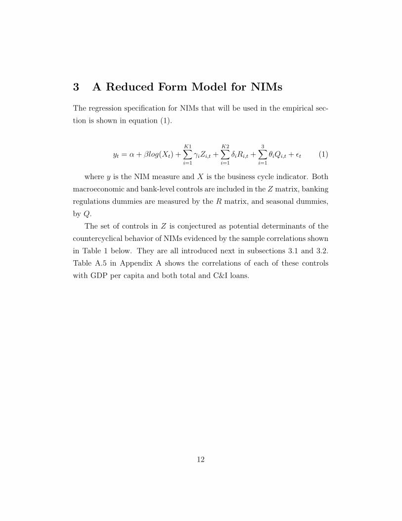
3 A Reduced Form Model for NIMs
The regression specification for NIMs that will be used in the empirical sec-
tion is shown in equation (1).
yt = α + βlog(Xt) +K1∑i=1
γiZi,t +K2∑i=1
δiRi,t +3∑
i=1
θiQi,t + εt (1)
where y is the NIM measure and X is the business cycle indicator. Both
macroeconomic and bank-level controls are included in the Z matrix, banking
regulations dummies are measured by the R matrix, and seasonal dummies,
by Q.
The set of controls in Z is conjectured as potential determinants of the
countercyclical behavior of NIMs evidenced by the sample correlations shown
in Table 1 below. They are all introduced next in subsections 3.1 and 3.2.
Table A.5 in Appendix A shows the correlations of each of these controls
with GDP per capita and both total and C&I loans.
12
3.1 Explaining the Countercyclicality: Macroeconomic
Determinants
Monetary Policy:
Several measures for the stance of monetary policy have been suggested
in the literature. The “Romer dates” type of measures (Romer and Romer,
1990 and Boschen and Mills, 1991) look at the monetary authority decisions
through its Federal Open Market Committee minutes. However, as pointed
out in Kashyap, Stein and Wilcox (1993), this implies looking at just a few
isolated episodes and valuable information can be lost this way. Alternatively,
Bernanke and Blinder (1992) argue that the federal funds rate is a fairly good
indicator. Thus, this last measure is used here.
The expected effect of the federal funds rate on NIMs needs to be assessed
first. As suggested in Angelini and Cetorelli (2003), interest rates on banks
liabilities are characterized by more inertia than those on assets, so that
monetary policy shocks to interest rates should be associated with increased
margins. Hannan and Berger (1991) and Neumark and Sharpe (1992) also
find evidence for the rigidity of deposit rates.
Another rationale for a positive coefficient on the federal funds rate is
given by the bank lending channel of monetary policy (Kashyap, Stein and
Wilcox, 1993; Kashyap and Stein, 1997 and Kashyap and Stein, 2000). Banks
can react to a fall in reserves due to a contractionary monetary policy by
relying more on non-reservable liabilities, such as certificate of deposits, to
finance loans. However, these alternative funds are not covered by deposit
insurance17 and thus, banks may choose to not fully offset the effects of the
policy, and they may let lending fall as a result. This effect occurs on top
of the contraction in loans derived from a lower demand for credit. Spreads
can be expected to increase with lending falling. Kashyap and Stein (2000)
17Leaving the bank exposed to credit risk
13
argue that under the lending view of monetary policy, the Federal Reserve
can affect not only Treasury bill rates but also the effective NIM.
Next, with this positive effect of the federal funds rate on NIMs in mind,
the role played by monetary policy in determining the cyclicality of NIMs
has to be considered. Changes to the quantity of money and hence to the in-
terest rate exert two opposing forces on the cyclical behavior of spreads. On
the one hand, the level of economic activity is partly the result of monetary
policy. When output is high (low) as a result of an expansionary (contrac-
tionary) monetary policy, the federal funds rate and NIMs are low (high),
and monetary policy explains the countercyclicality of the spreads. On the
other hand, with monetary policy playing a stabilization role, an increase (a
fall) in the federal funds rate during a boom (recession) will cause NIMs to
increase (decrease). In this case, the countercyclicality of NIMs should be
explained with the help of factors other than monetary policy, as it would
imply procyclical NIMs.
While the level of economic activity is expected to respond with lags to
monetary changes, the federal funds rate is likely to react instantaneously
to the cyclical movements of the economy. Thus, to thoroughly account for
the effects of monetary policy, both the current and the lagged values of the
federal funds rate are used as controls. Up to four lags of the federal funds
rate were also included in the regression as a robustness check. This implied
no important changes in our results18.
Additionally, two different interaction variables are constructed with the
goal of appropriately measuring the total impact of monetary policy on bank
margins.
The first is built as the product of a measure of the liquidity of banks
balance sheets19 and the federal funds rate. Gibson (1996) finds that the
18See Appendix C for a discussion of this robustness check.19The liquidity measure used is the same that is included later as a bank-level determi-
14
macroeconomic effects of monetary policy are stronger when banks in the
aggregate hold less liquid portfolios. In their cross-sectional study, Kashyap
and Stein (2000) find that the impact of monetary policy on lending is weaker
for banks with more liquid balance sheets, as they can react to a fall in re-
serves due to a contractionary monetary policy and protect their loan port-
folios by drawing from the buffer of cash and securities. They find this to
happen mainly for small banks that do not have access to alternative unin-
sured external financing. For them the liquidity of the balance sheet is key
to determine their response to the policy shock. Conversely, for larger banks,
they find a positive and significant effect of liquidity on the strength of mon-
etary policy. Aggregate data for the entire size distribution of banks is used
in this study, and bigger banks with almost to perfect access to uninsured
sources of finance are more heavily weighted. Therefore, our results can be
expected to reproduce theirs for the case of big banks.
The second variable is the interaction between a concentration measure
given by the Herfindahl-Hirschman index in the market for total loans and
the federal funds rate. Peltzman (1969) develops a theoretical model that
relates market structure in banking to the transmission of monetary policy.
Cottarelli and Kourelis (1994) find that entry barriers slow policy transmis-
sion, although they do not find significant effects from differences in market
concentration. More recently, Adams and Amel (2005) study the relation-
ship between banking competition and the transmission of monetary policy
through the bank lending channel, and find that the impact of monetary
policy is weaker in more concentrated markets. Of course, the structure of
the banking industry does not change dramatically on a quarterly basis or
even at business cycle frequencies. Therefore, while we do expect a negative
sign for the coefficient on this regressor, we think it might be not significant.
nant of the cyclicality of NIMs.
15
Default or Credit Risk:
The lagged value of the net charge-off rate defined as loan charge-offs20
net of loan recoveries as a percentage of total loans is used as a measure of
the degree of default or credit risk in the economy.
Optimally chosen margins should be enough to cover the cost of increasing
the bank’s capital as risk exposure increases. Thus, an increase in the econ-
omy’s default rate on loans should imply an increase in the spread charged
by commercial banks. If, as expected, a higher credit risk is associated with
periods of low economic activity, default is a very important candidate to
explain the countercyclical behavior of spreads21.
However, we are not particularly concerned about risk with any of our
margin measures. All our margins use ex-post interest rates on loans, cal-
culated using the actual income obtained by banks after accounting for bad
loans. Actually, for these measures, a negative sign can be expected for the
coefficient on the risk variable. Angelini and Cetorelli (2003) use price-cost
margins similar to ours for the Italian banking sector and expect a negative
sign for the coefficient on the ratio of bad and doubtful loans to total assets.
An increase in the share of these loans can imply a fall in the income measure
used to compute ex-post NIMs. The spread between the bank prime and the
Treasury bill rates, also used as one of our margin measures, is an ex-ante
variable22. However, credit risk should not play an important role even in
20Charge-offs are the value of loans removed from the books and charged against loss
reserves.21The contemporaneous correlation of GDP per capita (GDPpc), total loans and com-
mercial and industrial (C&I) loans with the default measure are -0.21, 0.05 and 0.13,
respectively. With the lagged value of the charge-off they are -0.22, -0.13 and -0.01. See
Table A.5 in Appendix A.22It is calculated using cited interest rates series as opposed to banks actual interest
income.
16
this case. Both rates used to calculate this spread include only a small risk
premium, if any.
Alternative regressions were run where the delinquency rate23, the loss
rate24 and the Baa-Treasury bond spread25 were used as measures of default
risk. This implied no important qualitative differences with our results.
Interest Rate Risk:
Previous studies have shown both theoretically and empirically the impor-
tance of accounting for interest rate risk (Ho and Saunders (1981), Saunders
and Schumacher (2000) and Demirguc-Kunt, Laeven, and Levine (2004)).
The idea is that banks may charge a premium to hedge against this type of
risk.
Thus, the volatility of short-term interest rates is included among the
regressors as a proxy for the interest rate risk faced by banks. Following
Saunders and Schumacher (2000), the measure used is the standard deviation
over each quarter of the weekly series for the 3-month Treasury bill rate. If
the risk measure and NIMs are positively correlated, a countercyclical risk
measure can explain the countercyclicality of margins.
Both the contemporaneous and the lagged values are included based on
the fact that the lagged measure is the one that is negatively correlated at
business cycle frequencies with our business cycle indicators26. The volatility
of interest rates has been suggested as a useful leading indicator of economic
23According to the Federal Reserve’s definition, delinquent loans and leases are those
past due thirty days or more and still accruing interest as well as those in non-accrual
status.24Defined here as the ratio of loans loss allowances to total loans.25Stock and Watson (1990) suggest that this spread is a useful indicator of the default
risk prospects on private debt.26The volatility of the Treasury Bill rate is negatively correlated with GDP contempo-
raneously too.
17
activity. Interest rate volatility hampers investment and lowers consumer
confidence, exerting a negative effect on GDP levels. Thus, high volatility
increases the probability of a future recession. This explains the counter-
cyclicality of the volatility measure.
The Economy’s Financial Deepening:
An indicator of the degree of financial depth in the economy is included
among the controls.
A negative sign is expected for the coefficient on this regressor because
a deeper financial sector should imply a bigger availability of substitutes to
bank credit. Banks should therefore need to charge lower spreads.
Demirguc-Kunt and Huizinga (2000) show evidence that countries with
underdeveloped financial systems that move towards more development see
bank profitability and margins fall. However, once they control for bank
and market development, they cannot find independent effects on margins of
financial structure per se.
Following Kashyap, Stein and Wilcox (1993), this degree is measured as
the ratio of commercial paper issued by the nonfarm nonfinancial corpo-
rate business sector to the sum of commercial paper and bank loans for the
nonfarm nonfinancial corporate business and nonfarm noncorporate business
sectors. The lagged value of the variable is used, based on this measure
being more procyclical than the contemporaneous counterpart. With this
procyclicality and with a negative expected coefficient, the inclusion of fi-
nancial depth as a control should help in explaining the countercyclicality of
NIMs.
One explanation for the procyclicality can be found in Kashyap, Stein
and Wilcox (1993). They show that a monetary contraction makes this
financial deepening indicator increase as bank lending decreases by more
than commercial paper. Thus, high federal funds rates in periods of high
18
output levels (i.e. a countercyclical monetary policy) can explain the cyclical
pattern of this variable.
Supply of Funds:
The supply of deposits available to banks is used as a proxy for their
marginal cost of funds. Given that deposits are procyclical, the marginal cost
can be expected to be countercyclical. If costs and margins are positively
related, this can provide an explanation for countercyclical NIMs27.
Inflation:
Banks might require higher risk premia when inflation or nominal interest
rates are high. Huybens and Smith (1999) argue that inflation may make
informational asymmetries stronger and lead to higher NIMs. Boyd, Levine
and Smith (2001) find a significant, economically important and negative re-
lationship between inflation and banking sector development. In turn, lower
development can be conjectured to derive in increased net interest margins.
Saunders and Schumacher (2000) present evidence for margins increasing
with higher interest rate volatility, which can be associated with high and
variable inflation. Demirguc-Kunt and Huizinga (2000) provide support to
the fact that banks profits increase in inflationary environments. Demirguc-
Kunt, Laeven and Levine (2004) show that inflation has a robust, positive
impact on bank margins and overhead costs. For Italy, Angelini and Cetorelli
(2003) document a negative effect of inflation on price-cost margins, though.
Therefore, changes in the consumer price index (CPI) are included as a
regressor even though all our variables are measured in real terms. Given
27It would be interesting to extend the paper by including alternative measures of the
operative costs of banks. Data on non-interest expenses, banks’ spending on furniture and
equipment and salaries and benefits are available from the Call Reports on Condition and
Income data.
19
the negative correlation between economic activity and inflation at business
cycle frequencies, a direct relationship between inflation and margins might
provide another explanation for the countercyclical behavior of the latter.
3.2 Explaining the Countercyclicality: Bank-Level Ex-
planations
Liquidity:
The ratio between cash and total investment securities to total assets
is introduced among our regressors as a measure of aggregate liquidity for
banks28.
Demirguc-Kunt, Laeven and Levine (2004) find evidence that banks with
more liquid assets have lower net interest margins. The intuition there is that
banks with high levels of liquid assets in cash and government securities may
receive lower interest income than banks with less liquid assets. If the market
for deposits is reasonably competitive, then greater liquidity will tend to be
negatively associated with interest margins. Angbazo (1997) finds that as
the proportion of funds invested in cash or cash equivalents increases, banks
liquidity risk29 declines and leads to a lower liquidity premium in net interest
margins.
On the contrary, it could also be argued that when banks choose to hold
28See data appendix for definition. Kashyap and Stein (1997) define liquidity for each
bank as the ratio of cash plus securities plus federal funds sold to total assets. Due to
the lack of data on federal funds for several periods, we depart slightly from them and
define it as cash plus securities over total assets. The aggregate measure is calculated as
the weighted average across banks, with the weights given by each bank’s share in total
assets for each period.29This is the risk of not having sufficient cash or borrowing capacity to meet deposit
withdrawals or new loan demand, thereby forcing banks to borrow emergency funds at
excessive cost. The analysis uses the ratio of liquid assets to liabilities to proxy for liquidity
risk.
20
more liquid portfolios, they pay for the cost of that liquidity by raising their
margins. Ho and Saunders (1981) and Saunders and Schumacher (2000) de-
velop a model where banks charge spreads that are mainly fees in order to
provide what they call “immediacy services”. Theirs is a dealership frame-
work where risk-averse banks charge a cost for the immediate provision of
deposits and loans. In their model banks have to temporarily invest funds
in the money market whenever a deposit arrives at a time different from a
new loan demand, and they face a reinvestment risk if the short term rate
falls. If banks face a demand for a new loan without a contemporaneous
supply of new deposits, they need to borrow temporarily in the money mar-
ket, facing a refinancing risk should the short term interest rate go up. The
spread compensates banks for bearing this risk. Holding more liquid assets
can be viewed as an alternative to having to resort to the money market to
provide these “immediacy services”. Therefore, we think this model provides
a rationale for a positive relationship between margins and banks liquidity.
If the positive effect of liquidity on NIMs is stronger, cyclical changes in
liquidity can provide another explanation for the countercyclicality of mar-
gins. This is because all our measures of economic activity and our liquidity
measure are negatively correlated. Therefore, more economic activity which
is related to lower liquidity, lowers the cost of it for banks and allows NIMs
to shrink.
The countercyclicality of balance sheet liquidity can be easily explained
by the fact that, in recessions, credit risk increases more for risky and illiquid
assets, such as loans, than for more liquid assets such as government securi-
ties. It is natural then to think that these risk-return considerations result
in banks shifting their asset portfolio toward more liquid assets during bad
times. Also, banks opportunity cost of holding more liquid and less profitable
assets falls in recessions when there are fewer investment opportunities.
21
Banks Capital Holdings:
Another control is the ratio of total equity capital to total loans. The
goal here is to control for the effect of capital requirements for banks. After
the Basle Accords of 1988 banks are required to hold a minimum of capital
as a percentage of risk weighted assets. However, the lack of data on risk
weighted assets for each bank prevent the use of that measure30. Total loans
are used instead bearing in mind that loans are one of the riskiest assets in
banks’ portfolios.
There is empirical evidence that banks hold capital against credit risk
in excess of the minimum 8% of total risk weighted assets required by the
Accords. In our sample equity represents 14% of loans. According to the
Bank of International Settlements, with the adoption of the Basle standards,
the average ratio of capital to risk-weighted assets of major banks in G-10
countries rose from 10% in 1988 to 11% in 1996.
Given that due mainly to taxation issues, holding equity is costly relative
to debt, banks may need to charge higher margins to finance this extra cost.
Hellman, Murdock and Stiglitz (2000) present a context that provides an
alternative story for capital requirements to increase margins. They show
that when capital requirements increase banks cost of funding, they lower
the franchise value of banks and this increases the incentives to excessive
risk-taking. Last, Demirguc-Kunt, Laeven and Levine (2004) argue that
highly capitalized banks have lower bankruptcy risks and lower funding costs
and that they therefore charge higher NIMs when interest rates on loans are
insensitive to equity.
The capital to assets ratio is countercyclical in our sample period. Thus, if
as expected an increase in the ratio implies an increase in margins, the inclu-
sion of this regressor in our set of controls can explain the countercyclicality
30Data on risk capital and risk-adjusted assets are available from the Report of Condition
and Income data only after 1991.
22
of margins.
The cyclical pattern of capital to assets ratio is the result of two opposing
forces. On the one hand, since loan default and delinquency rates tend
to increase during recessions, and since they both negatively affect banks
equity, the numerator of the ratio moves in a procyclical fashion. On the
other, demand for credit is highly procyclical and thus the ratio should move
countercyclically. As stated above, the second effect seems to dominate in
our sample.
The Share of Total Assets Held by Big Banks:
The share of total assets held by big banks is included among our controls
as a measure of concentration. The Herfindahl-Hirschman index (HHI) for
the market for loans is an alternative measure of concentration. Figures 1
and 2 show the comovement of the two measures. Two different measures for
the Herfindahl index are shown there: an aggregate measure and a weighted
average of states indexes. This distinction becomes specially relevant for
the pre-1997 period when interstate branching was not allowed in the US31.
Worthy of note is the important increase in all concentration measures over
the last years.
If higher market concentration is a good proxy for less competition, there
should be a positive relationship between market concentration and price-
31To understand the need for this adjustment, consider an economy where banks are
restricted to operate in only one state and where there is only one bank in each state. The
aggregate HHI in that economy would be∑
(1/N2) = 1/N with N being the number of
states. With the transformed measure, the weighted HHI would equal∑
(1 ∗ 1/N) = 1.
Therefore, the aggregate measure would be underestimating the concentration measure in
an economy where banks are perfect monopolies in each of their areas of operation. The
variability over time of these two measures can be expected to be different if the shares of
each state in total assets change significantly at business cycle frequencies. However, we
do not expect these changes to be very important.
23
cost margins. Also, for a given interest rate on loans, concentration will
increase NIMs if it allows banks to offer lower deposit rates. Berger and
Hannan (1989) provide strong evidence of a negative relationship between
market concentration and deposit rates. Hannan and Berger (1991) find that
banks in more concentrated markets have more rigid deposit rates, and that
deposit rates are stickier upwards than downwards. Neumark and Sharpe
(1992) find that in more concentrated markets deposit rates rise more slowly
and fall faster after a change in input costs. They also find that banks in
concentrated markets offer lower rates on deposits than more competitive
banks.
However, Jackson (1992 and 1997), Rhoades (1995) and Hannan (1997)
present models of oligopolistic competition alternative to Cournot, accord-
ing to which there might be an inverse relationship between spreads and
concentration indexes32. Jackson (1992) finds that the negative price (de-
posit interest rate)-concentration relationship in Berger and Hannan (1989)
is not consistent over the full range of observed market concentration values.
Smirlock (1985) argues that market concentration is not random, but the
result of more efficient banks “endogenously” gaining larger market shares.
Therefore, he tests the hypothesis that there is no causal relationship be-
tween concentration and profitability in banking, but rather between market
share and profits. He does find a link of profits to market share, but no
positive relationship with concentration once this is controlled for.
32The basic idea in these models is that banks operate in a perfectly competitive market
for loans, but have market power when getting deposits from savers in the economy and
they choose the interest rate on deposits. Their model of consumer deposit pricing is
represented by a general rational distributed lag function. The change in the rate of
deposits is a function of the changes in the six-month Treasury bill rate at 0,...,N lags.
In this model, more concentrated markets should have higher spreads, but they would
also exhibit relatively more deposit rate rigidity. Jackson (1997) provides evidence of a
non-monotonic relationship between market concentration and price rigidity.
24
Also, the share of total bank assets held by big banks is not only a measure
of concentration, but one of the relative importance of bigger banks in the
economy. It can therefore capture differences, if any, in the behavior of these
banks relative to the rest. Flannery (1981) provides evidence that larger
banks charge lower margins. He shows that large banks effectively hedge
themselves against market rate risk by holding assets and liabilities of similar
average maturities. This provides a rationale why larger banks might charge
smaller margins. Ho and Sunders (1981) also show that smaller banks have
a one third of a percent larger spread than bigger banks.
Thus, it is not clear what sign to expect for this coefficient. If the negative
effect is stronger, the high procyclicality of the share observed in our sample
provides an alternative explanation for a countercyclical behavior of margins.
Two explanations for the high procyclicality of this variable are based on
the non-competitive behavior of large banks over the cycle. First, in a setting
of imperfect competition originated in product differentiation, we can think
of big banks being more aggressive than smaller banks in capturing most
of the increased demand for credit in booms. This can be done by invest-
ing more aggressively in advertising or differentiating from smaller banks by
offering other banking services together with loans, for example. A second
explanation can be found in a setting of strategic behavior of big banks as in
a colluding oligopoly along the lines of Rotemberg and Saloner (1986). Dur-
ing booms players revert to the non-collusion equilibrium with lower prices
and higher quantities. If the larger banks in the industry are the ones that
implicitly collude while smaller banks do not have such a strategic behavior,
then big banks will expand their share of the market during booms when the
collusion is more difficult to sustain.
25
3.3 Banking Regulation
A set of dummy variables is included in the regression specification to control
for three important regulatory changes that have taken place in the United
States banking sector during our sample period.
First, in 1980 the Depository Institutions Deregulation and Monetary
Control Act of 1980 eliminated the deposit interest rate ceilings imposed by
Regulation Q33 and increased the limit of deposit insurance by the FDIC
from $40,000 to $100,000 per account.
Second, in 1994 the Riegle-Neal Interstate Banking and Branching Effi-
ciency Act repealed the Douglas Amendment. It allowed national banks to
operate branches across state lines after June 1, 1997. The Riegle-Neal Act
specified that state law continues to control intrastate branching for both
national and state banks.
Third, the Gramm-Leach-Bliley Act (GLBA) enacted in November of
1999 increased the activities allowed for banks and their holding companies.
Before 1999 commercial banks were prevented from expanding into a wide
range of financial services such as investment banking. Specifically, they
could not hold corporate equity, and the underwriting of securities was left
to investment banks. The GLBA repealed the parts of the Banking Act of
1933 that separated commercial banking from the securities business, which
have come to be known as “Glass-Steagall”. It also repealed the parts of the
Bank Holding Company Act of 1956 that separated commercial banking from
the insurance business. Thus, the GLBA permits single holding companies
to offer banking, securities, and insurance, as they had before the Great
Depression (Barth et al., 2000).
33The prohibition against payment of interest on demand deposits is the last vestige of
Regulation Q that is still valid.
26
4 Empirical Methodology
4.1 The Data
The study uses time series quarterly data for the period 1979:I-2005:I. Bank-
level balance sheet and income data is taken from the Call Reports on Con-
dition and Income data, available for all banks regulated by the Federal Re-
serve System, Federal Deposit Insurance Corporation, and the Comptroller
of the Currency. These data are available from the Federal Reserve Bank
of Chicago. Details on variable definitions and sources can be found in Ap-
pendix A.
Eight alternative definitions are used here for NIMs. All the series are
shown in Figure 3. In only one case macro data is used to calculate the spread
as the difference between the bank prime and the Treasury bill rates. The
latter is taken as a proxy for the interest rate on deposits paid by commercial
banks. Dueker and Thornton (1997) also use the bank prime as the lending
rate in their study of markups in the banking sector. They argue that a
change in the prime rate is indicative of a general shift in lending rates.
It is important to state here the distinction between spreads and net
interest margins. The pure spread is the rate spread between loan and deposit
rates. NIMs are calculated as the ratio of the difference between interest
revenues and interest expenses to assets, whereas spreads are obtained as
the difference between interest returns (i.e., interest revenues/earning assets)
and interest costs (i.e., interest expenses minus provisions for loans losses,
divided by interest bearing liabilities) (Angbazo, 1997). In this sense, our
NIMs 1,2 and 3 as well as C&I 1 and 2 more closely measure spreads, while
NIM 4 and 5 are strictly “margins” and comparable to the measures that the
previous literature has worked with34.
34Demirguc-Kunt, Laeven and Levine (2004) define the net interest margin as interest
income minus interest expense divided by interest-bearing assets. In Angbazo (1997) the
27
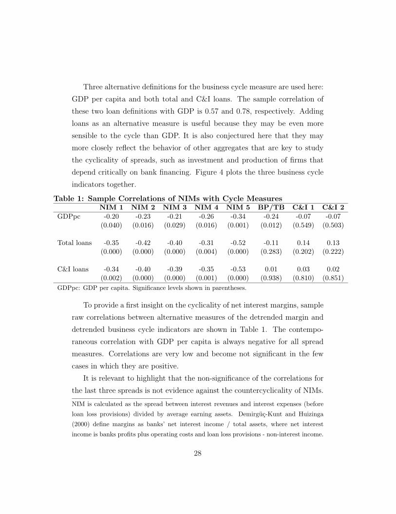
Three alternative definitions for the business cycle measure are used here:
GDP per capita and both total and C&I loans. The sample correlation of
these two loan definitions with GDP is 0.57 and 0.78, respectively. Adding
loans as an alternative measure is useful because they may be even more
sensible to the cycle than GDP. It is also conjectured here that they may
more closely reflect the behavior of other aggregates that are key to study
the cyclicality of spreads, such as investment and production of firms that
depend critically on bank financing. Figure 4 plots the three business cycle
indicators together.
Table 1: Sample Correlations of NIMs with Cycle MeasuresNIM 1 NIM 2 NIM 3 NIM 4 NIM 5 BP/TB C&I 1 C&I 2
GDPpc -0.20 -0.23 -0.21 -0.26 -0.34 -0.24 -0.07 -0.07(0.040) (0.016) (0.029) (0.016) (0.001) (0.012) (0.549) (0.503)
Total loans -0.35 -0.42 -0.40 -0.31 -0.52 -0.11 0.14 0.13(0.000) (0.000) (0.000) (0.004) (0.000) (0.283) (0.202) (0.222)
C&I loans -0.34 -0.40 -0.39 -0.35 -0.53 0.01 0.03 0.02(0.002) (0.000) (0.000) (0.001) (0.000) (0.938) (0.810) (0.851)
GDPpc: GDP per capita. Significance levels shown in parentheses.
To provide a first insight on the cyclicality of net interest margins, sample
raw correlations between alternative measures of the detrended margin and
detrended business cycle indicators are shown in Table 1. The contempo-
raneous correlation with GDP per capita is always negative for all spread
measures. Correlations are very low and become not significant in the few
cases in which they are positive.
It is relevant to highlight that the non-significance of the correlations for
the last three spreads is not evidence against the countercyclicality of NIMs.
NIM is calculated as the spread between interest revenues and interest expenses (before
loan loss provisions) divided by average earning assets. Demirguc-Kunt and Huizinga
(2000) define margins as banks’ net interest income / total assets, where net interest
income is banks profits plus operating costs and loan loss provisions - non-interest income.
28

Several forces like changes in banking regulation and seasonality of the data
not accounted for in these raw correlations may be distorting the picture. It
will be shown below that when controlling for the effects of banking regulation
and seasonality as well as monetary policy and default risk, the coefficient on
the business cycle indicator becomes negative and significant in all 24 cases.
4.2 Estimation Strategy
Augmented Dickey-Fuller (ADF) tests were run for all the variables in our
sample to test for the presence of unit roots. Except in a few cases, we do
not have a priori on the process followed by each variable under the null of a
unit root. Thus, we preferred to follow the methodology put forth by Dolado,
Jenkinson and Sosvilla-Rivero (1990)35. The optimal lag length for the ADF
regressions was based on the Akaike Information Criterion and the Schwartz
Bayesian criterion as well as on the Box-Pierce Q test for white noise of the
errors of the regression. Table A.5 in Appendix A shows the results of the
stationarity checks performed.
When detected, non-stationarity was dealt with by transforming the orig-
inal series into stationary processes. Trend stationary (TS) variables were
detrended by regressing them on a constant and a polynomial of time36. Dif-
ference stationary (DS) variables were also “detrended” using the Hodrick-
Prescott filter with a smoothing parameter of 1600 to separate the cyclical
component from trend. All detrended variables were proven to be stationary
35In short, the methodology starts with an unrestricted model that includes a constantand trend and then tests sequentially for the validity of the trend first and for the constantlater. If in any of the three possible models the null of unit root is not rejected, thenthe variable is difference stationary (DS) with drift plus trend, DS with drift or DS,respectively. If the null is rejected at some stage, then we can conclude the variable beingtrend stationary (TS). The advantage of this method is that once the “true” model isknown under the null, the power of the unit root test can be increased by using the usualt-test instead of the values tabulated by Dickey and Fuller (this result is due to Sims,Stock and Watson, 1990).
36The order of the polynomial was chosen based on fit.
29
by rejecting Dickey-Fuller tests. The original model was thus redefined in
terms of these detrended stationary variables.
DS variables were not first-differenced because we think that including
the first-differenced variables in the model would both be methodologically
incorrect and lack economic meaning. From the point of view of econometric
theory, it would be wrong to try to estimate the original parameters from
the model in levels by first-differencing all the variables when some of them
are TS rather than DS. An alternative would be to redefine the original
model in terms of a mixture of first-differenced DS variables and detrended
TS variables. However, for the purpose of measuring the cyclical pattern
followed by spreads it is necessary to isolate the business cycle frequency
component of the explanatory variables. Quarterly changes in GDPpc or in
total loans may or may not be related to the phase of the business cycle.
That is, the estimated coefficients on these first-difference variables could
not clearly be interpreted as measures of the countercyclicality of spreads.
The specification includes lags of some of the independent variables.
Lagged dependent variables are not included because we consider they do
not belong to the econometric model. Of course, important autocorrelation
in the disturbances is expected, so two tests for autocorrelation are imple-
mented here. Durbin-Watson (DW) test for first-order autocorrelation and
also Breusch-Godfrey (BG) test for possible autocorrelation of up to order
4. It has been suggested that an AR(4) model is appropriate for quarterly
data because of seasonal autocorrelation. Indeed, in several cases the null
of no autocorrelation cannot be rejected with the DW statistic, but it is re-
jected when using the BG test (see Table 4 and tables B.1-B.6 in Appendix
B). In all cases in which some form of autocorrelation was found, standard
errors were obtained by using the Newey-West robust, consistent estimator
for autocorrelated disturbances of unspecified structure.
Our specification also presents potential endogeneity problems. A system
30
of equations bias can be affecting our results if, as expected, some of the ex-
planatory variables in the basic specification are simultaneously determined
with the dependent variable. Specially prone to this bias are the business
cycle indicator and the share of total assets held by big banks37.
To account for endogeneity, the models were also estimated by two-stage
least squares (2SLS)38. Since IV methods are relatively inefficient compared
to OLS, a Hausman specification test was run in order to evaluate the com-
promise between efficiency and consistency of our estimations.
Finally, variance inflation factor (VIF) tests were run on our regressions
to check for the existence of multicollinearity.
5 Results
The results for the estimations obtained following the methodology outlined
in Section 4 are presented in this section.
Monetary policy and default risk are the two main candidates to explain
the countercyclicality indicated by the sample correlations shown in Table 1.
In order to study if the cyclicality of margins is robust to these important
determinants, they are both introduced as controls in our basic specification.
The basic specification also includes dummies to control for the effect of
regulatory changes in the banking sector that took place during our sample
period. Also, since most of our data is not seasonally adjusted, quarterly
dummies are included to capture any seasonality affecting banks margins.
As a robustness check, the cyclical behavior of NIMs was also studied
37When thought of as a measure of concentration, this share might itself be a functionof the spread.
38Three-stage least squares (3SLS) would have allowed for correlation among the errorterms of the three equations: the margin, the cycle indicator and the share of big banksin total assets. 3SLS gives more efficient estimates, but 2SLS ones are still consistent.Moreover, 3SLS would pose the risk that a wrongly specified equation bias the estimatorsof interest in the NIM equation.
31
when not controlling for monetary policy and default risk. All the NIMs
measures were regressed against each of the three alternative business cycle
indicators and just the dummies controlling for regulations and seasonality
in the data. The results can be found in Appendix C. Overall, the counter-
cyclicality of NIMs is robust to this change in the econometric specification.
A set of additional regressors is added later to the basic specification.
The main goal there is to try to explain the actual channels through which
macroeconomic aggregates such as GDP affect the microeconomic behavior
of banks, and generate countercyclical NIMs. Thus, no explanatory power
should be left to the cycle measure after including this expanded set of con-
trols.
5.1 Regressions with Basic Controls
Results for the basic specification are summarized in Table 2. The counter-
cyclicality of spreads is documented with a negative and significant coefficient
on all business cycle indicators and for all definitions of NIMs. The result is
robust to the inclusion of dummy variables to control for both banking regu-
lation issues and seasonality in the data. This is true even after controlling for
the effects of countercyclical monetary policy and default risk. Importantly,
the coefficients on the margins on C&I loans and the bank prime-Treasury
bill spread become significantly different from zero, even when the sample
raw correlations presented in Table 1 are not.
The full regression output along with several important regression diag-
nostic statistics are shown in Tables B.1 to B.3 of Appendix B. The coeffi-
cients for seasonal and regulation dummies were not included in those tables.
The stance of monetary policy is measured with the federal funds rate, in-
cluding both the current rate and a lagged value. Credit risk was accounted
for with a lagged value of the net charge-off rate.
32
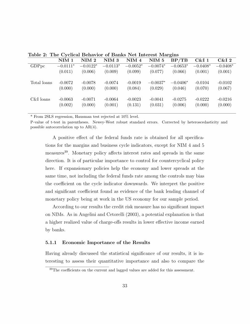
Table 2: The Cyclical Behavior of Banks Net Interest MarginsNIM 1 NIM 2 NIM 3 NIM 4 NIM 5 BP/TB C&I 1 C&I 2
GDPpc −0.0111∗ −0.0122∗ −0.0113∗ −0.0052∗ −0.0074∗ −0.0653∗ −0.0408∗ −0.0408∗
(0.011) (0.006) (0.009) (0.099) (0.077) (0.066) (0.001) (0.001)
Total loans -0.0072 -0.0078 -0.0074 -0.0019 −0.0037∗ −0.0406∗ -0.0104 -0.0102(0.000) (0.000) (0.000) (0.084) (0.029) (0.046) (0.070) (0.067)
C&I loans -0.0063 -0.0071 -0.0064 -0.0023 -0.0041 -0.0275 -0.0222 -0.0216(0.002) (0.000) (0.001) (0.131) (0.031) (0.006) (0.000) (0.000)
* From 2SLS regression, Hausman test rejected at 10% level.P-value of t-test in parentheses. Newey-West robust standard errors. Corrected by heteroscedasticity andpossible autocorrelation up to AR(4).
A positive effect of the federal funds rate is obtained for all specifica-
tions for the margins and business cycle indicators, except for NIM 4 and 5
measures39. Monetary policy affects interest rates and spreads in the same
direction. It is of particular importance to control for countercyclical policy
here. If expansionary policies help the economy and lower spreads at the
same time, not including the federal funds rate among the controls may bias
the coefficient on the cycle indicator downwards. We interpret the positive
and significant coefficient found as evidence of the bank lending channel of
monetary policy being at work in the US economy for our sample period.
According to our results the credit risk measure has no significant impact
on NIMs. As in Angelini and Cetorelli (2003), a potential explanation is that
a higher realized value of charge-offs results in lower effective income earned
by banks.
5.1.1 Economic Importance of the Results
Having already discussed the statistical significance of our results, it is in-
teresting to assess their quantitative importance and also to compare the
39The coefficients on the current and lagged values are added for this assessment.
33
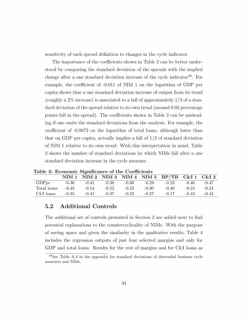
sensitivity of each spread definition to changes in the cycle indicator.
The importance of the coefficients shown in Table 2 can be better under-
stood by comparing the standard deviation of the spreads with the implied
change after a one standard deviation increase of the cycle indicator40. For
example, the coefficient of -0.011 of NIM 1 on the logarithm of GDP per
capita shows that a one standard deviation increase of output from its trend
(roughly a 2% increase) is associated to a fall of approximately 1/3 of a stan-
dard deviation of the spread relative to its own trend (around 0.02 percentage
points fall in the spread). The coefficients shown in Table 2 can be mislead-
ing if one omits the standard deviations from the analysis. For example, the
coefficient of -0.0072 on the logarithm of total loans, although lower than
that on GDP per capita, actually implies a fall of 1/2 of standard deviation
of NIM 1 relative to its own trend. With this interpretation in mind, Table
3 shows the number of standard deviations by which NIMs fall after a one
standard deviation increase in the cycle measure.
Table 3: Economic Significance of the CoefficientsNIM 1 NIM 2 NIM 3 NIM 4 NIM 5 BP/TB C&I 1 C&I 2
GDPpc -0.36 -0.41 -0.38 -0.30 -0.29 -0.23 -0.46 -0.47Total loans -0.48 -0.54 -0.52 -0.23 -0.30 -0.30 -0.24 -0.24C&I loans -0.35 -0.41 -0.37 -0.23 -0.27 -0.17 -0.43 -0.43
5.2 Additional Controls
The additional set of controls presented in Section 3 are added next to find
potential explanations to the countercyclicality of NIMs. With the purpose
of saving space and given the similarity in the qualitative results, Table 4
includes the regression outputs of just four selected margins and only for
GDP and total loans. Results for the rest of margins and for C&I loans as
40See Table A.4 in the appendix for standard deviations of detrended business cyclemeasures and NIMs.
34
well as a number of regression diagnostic tests are all included in Tables B.4
to B.6 of Appendix B.
For all regressions in Table 4 and also in Tables B.4 to B.6, the cycle
measure completely loses its explanatory power41. This evidence suggests
that at least a subset of the included controls are important channels through
which fluctuations in the economy translate into cyclical movements of the
spreads.
Overall, the federal funds rate retains its positive and significant impact
on spreads even after introducing the additional controls. Moreover, in the
case in which the coefficient on the contemporaneous rate is negative, the
total effect of monetary policy on NIMs is still positive when considering the
rate’s lagged value42.
41The only exception corresponds to the particular case of NIMs C&I 1 and C&I 2 withC&I loans, for which the quantity indicator keeps its significance and negative sign.
42The only exception is given by the combinations of NIM 5 with GDP and with C&Iloans. Monetary policy exerts a negative effect on NIMs in these two cases.
35
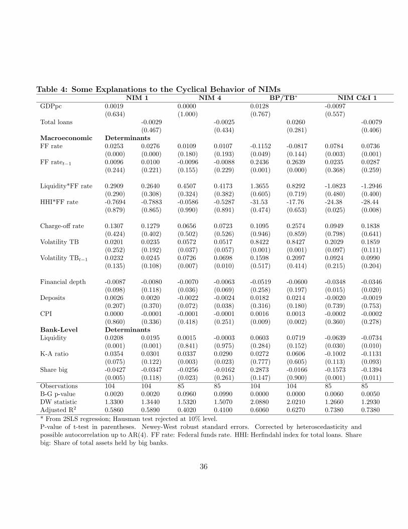
Table 4: Some Explanations to the Cyclical Behavior of NIMsNIM 1 NIM 4 BP/TB∗ NIM C&I 1
GDPpc 0.0019 0.0000 0.0128 -0.0097(0.634) (1.000) (0.767) (0.557)
Total loans -0.0029 -0.0025 0.0260 -0.0079(0.467) (0.434) (0.281) (0.406)
Macroeconomic DeterminantsFF rate 0.0253 0.0276 0.0109 0.0107 -0.1152 -0.0817 0.0784 0.0736
(0.000) (0.000) (0.180) (0.193) (0.049) (0.144) (0.003) (0.001)FF ratet−1 0.0096 0.0100 -0.0096 -0.0088 0.2436 0.2639 0.0235 0.0287
(0.244) (0.221) (0.155) (0.229) (0.001) (0.000) (0.368) (0.259)
Liquidity*FF rate 0.2909 0.2640 0.4507 0.4173 1.3655 0.8292 -1.0823 -1.2946(0.290) (0.308) (0.324) (0.382) (0.605) (0.719) (0.480) (0.400)
HHI*FF rate -0.7694 -0.7883 -0.0586 -0.5287 -31.53 -17.76 -24.38 -28.44(0.879) (0.865) (0.990) (0.891) (0.474) (0.653) (0.025) (0.008)
Charge-off rate 0.1307 0.1279 0.0656 0.0723 0.1095 0.2574 0.0949 0.1838(0.424) (0.402) (0.502) (0.526) (0.946) (0.859) (0.798) (0.641)
Volatility TB 0.0201 0.0235 0.0572 0.0517 0.8422 0.8427 0.2029 0.1859(0.252) (0.192) (0.037) (0.057) (0.001) (0.001) (0.097) (0.111)
Volatility TBt−1 0.0232 0.0245 0.0726 0.0698 0.1598 0.2097 0.0924 0.0990(0.135) (0.108) (0.007) (0.010) (0.517) (0.414) (0.215) (0.204)
Financial depth -0.0087 -0.0080 -0.0070 -0.0063 -0.0519 -0.0600 -0.0348 -0.0346(0.098) (0.118) (0.036) (0.069) (0.258) (0.197) (0.015) (0.020)
Deposits 0.0026 0.0020 -0.0022 -0.0024 0.0182 0.0214 -0.0020 -0.0019(0.207) (0.370) (0.072) (0.038) (0.316) (0.180) (0.739) (0.753)
CPI 0.0000 -0.0001 -0.0001 -0.0001 0.0016 0.0013 -0.0002 -0.0002(0.860) (0.336) (0.418) (0.251) (0.009) (0.002) (0.360) (0.278)
Bank-Level DeterminantsLiquidity 0.0208 0.0195 0.0015 -0.0003 0.0603 0.0719 -0.0639 -0.0734
(0.001) (0.001) (0.841) (0.975) (0.284) (0.152) (0.030) (0.010)K-A ratio 0.0354 0.0301 0.0337 0.0290 0.0272 0.0606 -0.1002 -0.1131
(0.075) (0.122) (0.003) (0.023) (0.777) (0.605) (0.113) (0.093)Share big -0.0427 -0.0347 -0.0256 -0.0162 0.2873 -0.0166 -0.1573 -0.1394
(0.005) (0.118) (0.023) (0.261) (0.147) (0.900) (0.001) (0.011)Observations 104 104 85 85 104 104 85 85B-G p-value 0.0020 0.0020 0.0960 0.0990 0.0000 0.0000 0.0060 0.0050DW statistic 1.3300 1.3440 1.5320 1.5070 2.0880 2.0210 1.2660 1.2930Adjusted R2 0.5860 0.5890 0.4020 0.4100 0.6060 0.6270 0.7380 0.7380* From 2SLS regression; Hausman test rejected at 10% level.P-value of t-test in parentheses. Newey-West robust standard errors. Corrected by heteroscedasticity andpossible autocorrelation up to AR(4). FF rate: Federal funds rate. HHI: Herfindahl index for total loans. Sharebig: Share of total assets held by big banks.
36
Our results cannot provide full support to the effect studied in Kashyap
and Stein (2000) related to the interaction between monetary policy and
banks liquidity. This hypothesis would imply a negative sign for the in-
teraction between liquidity and the federal funds rate. Coefficients are not
significant in all possible combinations of NIMs and cycle indicators. More-
over, consistently across business cycle measures, they are positive for all
NIMs except for the ones on C&I loans. However, our findings can be easily
reconciled with theirs recalling that their hypothesis is specially relevant for
small banks that typically have less than perfect access to uninsured sources
of finance. For larger banks they also find a positive and even significant
effect of this interaction on banks loan supply. In our aggregate data, large
banks43 weight more heavily than small and medium size banks, so we expect
the coefficient on this interaction to be at least positive and insignificant.
The coefficient obtained for the interaction between our measures of mon-
etary policy and concentration is negative and significant for the case of NIMs
on C&I loans. This provides support to the hypothesis on the weaker effect of
monetary policy when concentration increases in the banking industry. The
evidence found is weak though, because although the coefficients are still
negative, they are not significant any more for most other spread variables.
Concerning credit risk, although positive, the coefficients on the lagged
value of the charge-off rate are not significant. However, as discussed before,
we are not particularly concerned about risk with any of our ex-post margins.
Moreover, the spread between the bank prime and the Treasury Bill rates is
calculated using two interest rate measures that should, by definition, include
a very small risk premium, if any. Thus, even in this case we do not expect
a significantly positive effect of our credit risk measure.
Interest rate risk has a positive and in most cases significant impact on
43Bank size was determined in the same way than in Kashyap and Stein, 1997. Largebanks are those in the 99-100th percentile of total asset distribution, medium size banksare those in the 95-99th percentiles and the rest are small banks.
37
NIMs. Therefore, our conclusions are consistent with Ho and Saunders (1981)
theoretical model and with previous empirical studies that show NIMs in-
cluding an interest rate risk premium.
Although not significant in some cases, the financial depth measure exerts
a negative effect on the dependent variable, as expected.
The supply of deposits faced by banks and used as a proxy for the
marginal cost of funds for them does not have a consistently significant im-
pact on margins. Nevertheless, in some cases the sign is negative and signif-
icant as expected. Future research could try to incorporate more accurate
microeconomic measures of operative costs for banks.
Inflation rates do not seem to significantly affect banks price-cost margins.
However, significantly across cycle indicators, inflation has a positive and
significant impact on the spread between the bank prime and the treasury
bill rates.
The liquidity of banks portfolios increases margins for the case of NIMs 1-
3. In this sense, our results are consistent with those in Angbazo (1997) and
Demirguc-Kunt, Laeven and Levine (2004). However, no conclusive evidence
can be found as the coefficient is insignificant for other spreads and it is even
negative and significant for NIMs C&I.
The coefficient on the capital to assets ratio is positive and significant
across the different alternative specifications, except again for the case of the
spread on C&I loans. In general, banks seem to charge higher spreads to
cover the costs of capital holdings.
One explanation we can exercise for the fact that both banks liquidity
and capital holdings have a different impact on C&I margins is related to
the possibility available to banks of cross-subsidizing some product mixes.
This may affect the pricing of loans as suggested by Demirguc-Kunt, Laeven
and Levine (2004). C&I loans may be good candidates for these subsidies if
banks are subject to more competition in this market segment than in others
38
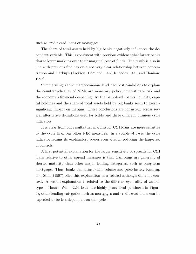
such as credit card loans or mortgages.
The share of total assets held by big banks negatively influences the de-
pendent variable. This is consistent with previous evidence that larger banks
charge lower markups over their marginal cost of funds. The result is also in
line with previous findings on a not very clear relationship between concen-
tration and markups (Jackson, 1992 and 1997, Rhoades 1995, and Hannan,
1997).
Summarizing, at the macroeconomic level, the best candidates to explain
the countercyclicality of NIMs are monetary policy, interest rate risk and
the economy’s financial deepening. At the bank-level, banks liquidity, capi-
tal holdings and the share of total assets held by big banks seem to exert a
significant impact on margins. These conclusions are consistent across sev-
eral alternative definitions used for NIMs and three different business cycle
indicators.
It is clear from our results that margins for C&I loans are more sensitive
to the cycle than our other NIM measures. In a couple of cases the cycle
indicator retains its explanatory power even after introducing the larger set
of controls.
A first potential explanation for the larger sensitivity of spreads for C&I
loans relative to other spread measures is that C&I loans are generally of
shorter maturity than other major lending categories, such as long-term
mortgages. Thus, banks can adjust their volume and price faster. Kashyap
and Stein (1997) offer this explanation in a related although different con-
text. A second explanation is related to the different cyclicality of various
types of loans. While C&I loans are highly procyclical (as shown in Figure
4), other lending categories such as mortgages and credit card loans can be
expected to be less dependent on the cycle.
39
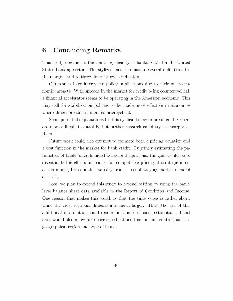
6 Concluding Remarks
This study documents the countercyclicality of banks NIMs for the United
States banking sector. The stylized fact is robust to several definitions for
the margins and to three different cycle indicators.
Our results have interesting policy implications due to their macroeco-
nomic impacts. With spreads in the market for credit being countercyclical,
a financial accelerator seems to be operating in the American economy. This
may call for stabilization policies to be made more effective in economies
where these spreads are more countercyclical.
Some potential explanations for this cyclical behavior are offered. Others
are more difficult to quantify, but further research could try to incorporate
them.
Future work could also attempt to estimate both a pricing equation and
a cost function in the market for bank credit. By jointly estimating the pa-
rameters of banks microfounded behavioral equations, the goal would be to
disentangle the effects on banks non-competitive pricing of strategic inter-
action among firms in the industry from those of varying market demand
elasticity.
Last, we plan to extend this study to a panel setting by using the bank-
level balance sheet data available in the Report of Condition and Income.
One reason that makes this worth is that the time series is rather short,
while the cross-sectional dimension is much larger. Thus, the use of this
additional information could render in a more efficient estimation. Panel
data would also allow for richer specifications that include controls such as
geographical region and type of banks.
40
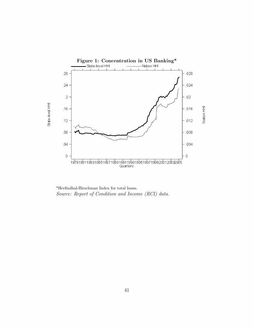
Figure 1: Concentration in US Banking*
*Herfindhal-Hirschman Index for total loans.Source: Report of Condition and Income (RCI) data.
41
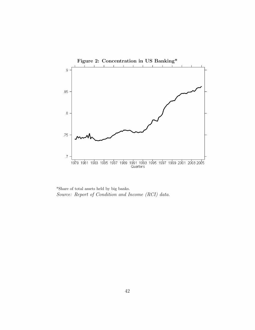
Figure 2: Concentration in US Banking*
*Share of total assets held by big banks.Source: Report of Condition and Income (RCI) data.
42
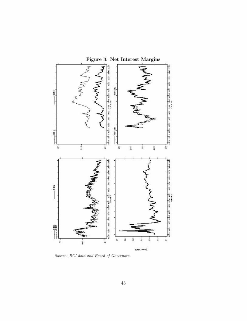
Figure 3: Net Interest Margins
Source: RCI data and Board of Governors.
43
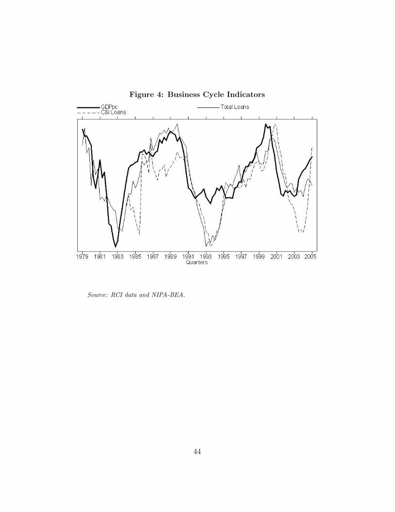
Figure 4: Business Cycle Indicators
Source: RCI data and NIPA-BEA.
44
References
[1] Adams. R. and D. Amel (2005), “The Effects of Local Banking MarketStructure on the Bank-Lending Channel of Monetary Policy”, Financeand Economics Discussion Series Papers, Board of Governors of theFederal Reserve System, 2005-16, April.
[2] Aggarwal, R. and K. Jacques (1998), “Assessing the Impact of PromptCorrective Action on Bank Capital and Risk”, Federal Reserve Bank ofNew York Economic Policy Review, October 23-32.
[3] Aliaga, R. (2005), “The General Equilibrium Dynamics of Banks CapitalAdequacy Regulation”, chapter 2 doctoral dissertation North CarolinaState University, May.
[4] Allen, L. (1988), “The Determinants of Bank Interest Margins: A Note”,Journal of Financial and Quantitative Analysis, Vol. 23, pp. 231-35.
[5] Angbazo, L. (1997), “Commercial Bank Net Interest Margins, DefaultRisk, Interest Rate Risk and Off-Balance Sheet Banking”, Journal ofBanking and Finance, Vol. 21, pp. 55-87. READ FOR A GOODSURVEY OF THE LITERATURE AT THE BEGINNING.
[6] Angelini, P. and N. Cetorelli (2000), “Bank Competition and Regu-latory Reform: The Case of the Italian Banking Industry”, Temi didiscussione, Banca d’Italia, working paper 380, October 2000.
[7] Angelini, P. and N. Cetorelli (2003), “The Effects of Regulatory Reformon Competition in the Banking Industry”, Journal of Money, Credit andBanking, Vol. 35 (5), October 2003, 663-684.
[8] Barth, J.,Brumbaugh, R. and Wilcox, J., “Policy Watch: The Repealof Glass-Steagall and the Advent of Broad Banking”, The Journal ofEconomic Perspectives, Vol. 14, No. 2, Spring 2000, pp. 191-204.
[9] Basle Committee on Banking Supervision (1999), “Capital Require-ments and Bank Behaviour: The Impact of the Basle Accord”, workingpaper N.1, Bank for International Settlements, Basle, Switzerland.
[10] Berg, Sigbjorn and Moshe Kim (1994), “Oligopolistic Interdependenceand the Structure of Production in Banking: An Empirical Evaluation”,Journal of Money, Credit and Banking, Vol. 26(2), May 1994, 309-322.
45
[11] Berg, S. and M. Kim, “Banks as Multioutput Oligopolies: An Empiri-cal Evaluation of the Retail and Corporate Banking Markets”, in BankStructure and Regulation, Conference Proceedings, Federal Reserve Bankof Chicago.
[12] Berger, A. (1995), “The Profit-Structure Relationship in Banking - Testsof Market Power and Efficient-Structure Hypothesis”, Journal of Money,Credit and Banking, Vol. 27, pp. 404-31.
[13] Berger, A. and T. Hannan (1989), “The Price-Concentration Relation-ship in Banking”, The Review of Economics and Statistics, Vol. 71, May,pp. 291-99.
[14] Berger, A. and T. Hannan (1998), “The Efficiency Cost of Market Powerin the Banking Industry: A Test of the Quiet Life and Related Hypothe-ses”, Review of Economics and Statistics, Vol. 80, pp. 454-65.
[15] Berger, A., G. Hanweck and D. Humphrey (1987), “Competitive Viabil-ity in Banking: Scale, Scope and Product Mix Economies”, Journal ofMonetary Economics, Vol. 20, pp. 501-20.
[16] Berger, A. and G. Udell (1992), “Some evidence on the empirical sig-nificance of credit rationing”, Journal of Political Economy 100, pp.1047-1077.
[17] Bernanke, B. and A. Blinder (1992), “The Federal Funds Rate andthe Channels of Monetary Transmission”, American Economic Review,September, Vol. 82, pp. 901-21.
[18] Bloch, H. and M. Olive (2001), “Pricing Over the Cycle”, Review ofIndustrial Organization, Vol. 19, 99-108.
[19] Boschen, J. and L. Mills (1995), “The Effects of Countercyclical Policyon Money and Interest Rates: An Evaluation of Evidence from FOMCDocuments”, working paper 91-20, Federal Reserve Bank of Philadel-phia, 1995.
[20] Boyd, J., R. Levine, and B. Smith (2001), “The Impact of Inflation onFinancial Sector Performance”, Journal of Monetary Economics, Vol.47, pp. 221-48.
[21] Campello, M. (2003), “Capital Structure and Product Markets Interac-tions: Evidence from Business Cycles”, Journal of Financial Economics,Vol. 68, 353-378.
46
[22] Chevalier, J. and D. Scharfstein (1995), “Liquidity Constraints and theCyclical Behavior of Markups”, The American Economic Review, Vol.85(2), Papers and Proceedings of the Hundredth and Seventh AnnualMeeting of the American Economic Association, Washington DC, Jan-uary 6-8, May 1995, 390-396.
[23] Chevalier, J. and D. Scharfstein (1996), “Capital-Market Imperfectionsand Countercyclical Markups: Theory and Evidence”, The AmericanEconomic Review, Vol. 86(4), September 1996, 703-725.
[24] Coccorese, P. (2002), “Competition Among Dominant Firms in Concen-trated Markets: Evidence from the Italian Banking Industry”, workingpaper 89, Centre for Studies in Economics and Finance, November 2002.
[25] Cottarelli, C. and A. Kourelis (1994), “Financial Structure, LendingRates, and the Transmission Mechanism of Monetary Policy”, Interna-tional Monetary Fund Staff Papers, 41(4), pp. 587-623.
[26] Demirguc-Kunt, A. and H. Huizinga (2000), “Financial Structure andBank Profitability”, World Bank Policy Research Working Paper No.2430, August.
[27] Demirguc-Kunt, A., Laeven, L. and Levine, R. (2004),“Regulations,Market Structure, Institutions, and the Cost of Financial Intermedia-tion”, Journal of Money, Credit, and Banking, June 2004, Vol. 36, Iss.3, pp. 593.
[28] Dolado, J., T. Jenkinson and S. Sosvilla-Rivero (1990), “Cointegrationand Unit Roots”, Journal of Economic Surveys, Vol. 4, pp. 249-73.
[29] Domowitz, I., G. Hubbard and B. Petersen (1986), “Business Cyclesand the Relationship Between Concentration and Price-Cost Margins”,Rand Journal of Economics, Spring 1986, 17, 1-17.
[30] Dueker, M. and D. Thornton (1997), “Do Bank Loan Rates Exhibit aCountercyclical Mark-up?”, working paper series Federal Reserve Bankof St. Louis, 1997-004A.
[31] Enders, W., Applied Econometric Time Series, New York, John Wileyand Sons, 1995.
[32] Ennis, H., “On the Size Distribution of Banks, Economic Quarterly,Federal Reserve Bank of Richmond, volume 87/4, Fall 2001.
47
[33] Flannery, M. (1981), “Market Interest Rates and Commercial BankProfitability: An Empirical Investigation”, Journal of Finance, Decem-ber, pp. 1085-101.
[34] Forbes, S. and L. Mayne (1989), “A Friction Model of the Prime”, Jour-nal of Banking and Finance, Vol. 13, pp.127.
[35] Galeotti, M. and F. Schiantarelli (1998), “The Cyclicality of Markups ina Model with Adjustment Costs: Econometric Evidence for US Indus-try”, Oxford Bulletin of Economics and Statistics, Vol. 60 (2), 121-142.
[36] Gali, J. (1994) “Monopolistic Competition, Business Cycles, and theComposition of Aggregate Demand”, Journal of Economic Theory, Vol.63(1), 73-96.
[37] Gelfand, M. and P. Spiller (1987), “Entry Barriers and MultiproductOligopolies”, International Journal of Industrial Organization, 5, 101-113.
[38] Gertler, M., G. Hubbard and A. Kashyap, “Interest Rate Spreads, CreditConstraints and Investment Fluctuations: An Empirical Investigation”,in Financial Markets and Financial Crises, edited by Glenn Hubbard, aNBER Project Report, The University of Chicago Press, 1991.
[39] Gibson, M. (1996), “The Bank Lending Channel of Monetary PolicyTransmission: Evidence from a Model of Bank Behavior that Incorpo-rates Long-Term Customer Relationships”, International Finance Dis-cussion Paper Federal Reserve Board, number 584, June 1997.
[40] Greene, W., Econometric Analysis, 4th. edition, Prentice Hall, 2000.
[41] Hannan. T. (1997), “Market Share Inequality, the Number of Competi-tors and the HHI: An Examination of Bank Pricing”, Review of Indus-trial Organization, 12, 23-35.
[42] Hannan, T. and A. Berger (1991), “The Rigidity of Prices: Evidencefrom the Banking Industry”, American Economic Review, volume 81(4),pp. 938-45.
[43] Hatanaka, M.(1974),“An Efficient Estimator for the Dynamic Adjust-ment Model with Autocorrelated Errors”, Journal of Econometrics, Vol.2, pp. 199-220.
48
[44] Hellman, T., K. Murdock and J. Stiglitz (2000), “Liberalization, MoralHazard in Banking and Prudential Regulation: Are Capital Require-ments Enough?”, American Economic Review, March, pp. 147-65.
[45] Ho, T., and A. Saunders (1981), “The Determinants of Bank InterestMargins: Theory and Empirical Evidence”, Journal of Financial andQuantitative Analyses, Vol. 16, 581-600.
[46] Huybens, E., and B. Smith. (1999), “Inflation, Financial Markets, andLong-Run Real Activity”, Journal of Monetary Economics, Vol. 43, pp.283-315.
[47] Hylleberg, S., R. Engle, C. Granger, and B. Yoo (1990), “Seasonal Inte-gration and Cointegration”, Journal of Econometrics, Vol. 44, pp. 215-38.
[48] Jackson, W. III (1992), “The Price Concentration Relationship in Bank-ing: A Comment”, Review of Economics and Statistics, 74, 373-376.
[49] Jackson, W. III (1997), “Market Structure and the Speed of Adjustment:Evidence of Non-Monotonicity”, Review of Industrial Organization, 12,37-57.
[50] Karlan, D. and J. Zinman (2004), “The Price Elasticity of Demand forCredit: Evidence and Implications from a Randomized Field Experi-ment”, working paper Princeton University and Federal Reserve Bankof New York, June 2004.
[51] Kashyap, A. and J. Stein (1997), “What Do a Million Banks Have toSay About the Transmission of Monetary Policy?”, NBER working paperseries, working paper 6056, June 1997.
[52] Kashyap, A., and J. Stein (1997), “The Role of Banks in MonetaryPolicy: A Survey with Implications for the European Monetary Union”,Federal Reserve Bank of Chicago Economic Perspectives, September-October, pp. 2-18.
[53] Kashyap, A., and J. Stein (2000), “What Do a Million Observationson Banks Say About the Transmission of Monetary Policy?”, AmericanEconomic Review, 90(3), pp. 407-28.
[54] Kashyap, A., J. Stein and D. Wilcox (1993), “Monetary Policy andCredit Conditions: Evidence from the Composition of External Fi-nance”, American Economic Review, Vol. 83, Number 1, March, pp.78-98.
49
[55] Klemperer, P. (1995), “Competition when Consumers Have Switch-ing Costs: An Overview with Applications to Industrial Organization,Macroeconomics and International Trade”, Review of Economic Studies,Vol. 62, pp. 515-39.
[56] Laurenceson, J. (2004), “Banking Industry Liberalization, FranchiseValues and Deposits Mobilization: Evidence from International PanelData”, working paper University of Queensland, Australia.
[57] Lebow, D. (1992), “Imperfect Competition and Business Cycles: AnEmpirical Investigation”, Economic Inquiry, Vol. 30(1), January 1992,177-193.
[58] Lerner, E. (1981), “Discussion: The Determinants of Bank Interest Mar-gins: Theory and Empirical Evidence”, Journal of Financial and Quan-titative Analysis, Vol. 16, pp. 601-602.
[59] McShane, R. and I. Sharpe (1985), “A Time Series/Cross-Section Anal-ysis of the Determinants of Australian Trading Bank Loan/Deposit In-terest Margins: 1962-1981”, Journal of Banking and Finance, Vol. 9,pp. 115-36.
[60] Mishkin, F., “Asymmetric Information and Financial Crises: A Histor-ical Perspective”, in Financial Markets and Financial Crises, edited byGlenn Hubbard, a NBER Project Report, The University of ChicagoPress, 1991.
[61] Neumark, D. and S. Sharpe (1992), “Market Structure and the Natureof Price Rigidity: Evidence from the Market for Consumer Deposits”,Quarterly Journal of Economics, 107(2), pp. 657-80.
[62] Olivero, M. (2004), “The Puzzles on International Comovement: TheRole of International Trade and Non-Competitive Banking”, workingpaper, December 2004.
[63] Peltzman, S. (1969), “The Banking Structure and the Transmission ofMonetary Policy”, Journal of Finance, 24(3), pp. 387-411.
[64] Phelps, E. and S. Winter (1970), “Optimal Price Policy Under Atom-istic Competition”, in E. Phelps et al., Microeconomic Foundations ofEmployment and Inflation Theory. New York: Norton.
[65] Ravn, M., S. Schmitt-Grohe, M. Uribe (2005), “Deep Habits”, forth-coming Review of Economic Studies.
50
[66] Rhoades, S.A. (1995), “Market Share Inequality, the HHI and OtherMeasures of the Firm Composition of a Market”, Review of IndustrialOrganization, 10, 657-674.
[67] Romer, C. and D. Romer (1990), “New Evidence on the Monetary Trans-mission Mechanism”, Brookings Papers on Economic Activity, pp. 149-213.
[68] Rotemberg, J. and G. Saloner (1986), “A Supergame-Theoretic Modelof Price Wars During Booms”, The American Economic Review, Vol. 76(3), June 1986, 390-407.
[69] Rotemberg, J. and M. Woodford (1992), “Oligopolistic Pricing and theEffects of Aggregate Demand on Economic Activity”, Journal of Polit-ical Economy, 100, 1153-1207.
[70] Rotemberg, J. and M. Woodford (1995), “Dynamic General EquilibriumModels with Imperfectly Competitive Product Markets”, in Frontiers ofBusiness Cycle Research, Cooley (ed.), 1995, 243-293.
[71] Samuelson, P. (1945), “The Effect of Interest Rate Increases on theBanking System”, American Economic Review, Vol. 35, March.
[72] Saunders, A. and L. Schumacher (2000), “The Determinants of Bank In-terest Rate Margins: an International Study”, Journal of InternationalMoney and Finance, Vol. 19 (6), 813-832.
[73] Scherer, F. M., Industrial Market Structure and Economic Performance,2nd ed. Boston: Houghton-Mifflin, 1980. Shaffer, Sherrill (1993), “ATest of Competition in Canadian Banking”, Journal of Money, Creditand Banking, Vol. 25(1), February 1993, 49-61.
[74] Shaffer, S. (1993), “A Test of Competition in Canadian Banking”, Jour-nal of Money, Credit and Banking, Vol. 25(1), February 1993, 49-61.
[75] Sims, C., J. Stock and M. Watson (1990), “Inference in Linear TimeSeries Models with Some Unit Roots”, Econometrica, Vol. 58, No. 1,pp. 113-44.
[76] Smirlock, M. (1985), “Evidence on the (Non) Relationship Between Con-centration and Profitability in Banking”, Journal of Money, Credit, andBanking, Vol. 17, pp. 69-83.
51
[77] Spiller, P. and E. Favaro (1984), “The Effects of Entry Regulation onOligopolistic Interactions: The Uruguayan Banking Sector”, The RandJournal of Economics, 9, 305-327.
[78] Stock, J. and M. Watson (1990), “New Indexes of Coincident and Lead-ing Economic Indicators”, NBER Working Paper R1380, April 1990.
[79] Wong, K. (1997), “On the Determinants of Bank Interest Margins UnderCredit and Interest Rate Risks”, Journal of Banking and Finance, Vol.21, pp. 25171.
[80] Zarruk, E. (1989), “Bank Spreads with Uncertain Deposit Level andRisk Aversion”, Journal of Banking and Finance, Vol. 13, pp. 797-810.
[81] Zarruk, E. and J. Madura (1992), “Optimal Bank Interest Margins Un-
der Capital Regulation and Deposit Insurance”, Journal of Financial
and Quantitative Analysis, Vol. 27, pp. 143-49.
52
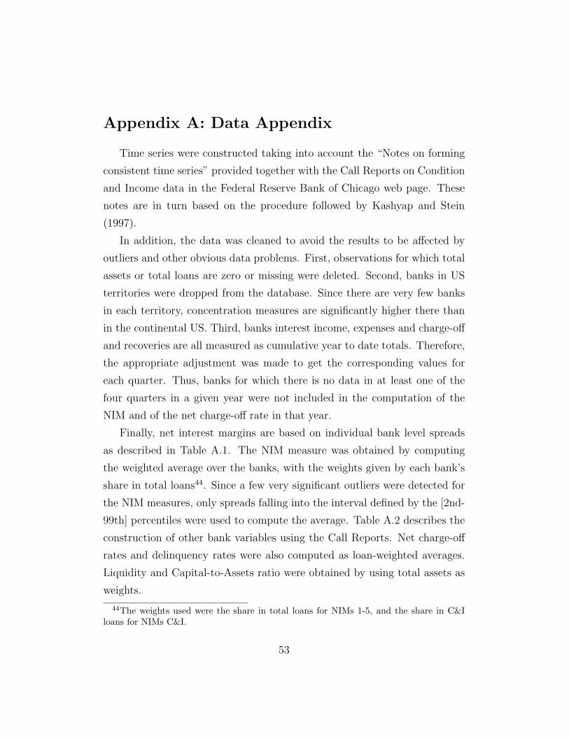
Appendix A: Data Appendix
Time series were constructed taking into account the “Notes on forming
consistent time series” provided together with the Call Reports on Condition
and Income data in the Federal Reserve Bank of Chicago web page. These
notes are in turn based on the procedure followed by Kashyap and Stein
(1997).
In addition, the data was cleaned to avoid the results to be affected by
outliers and other obvious data problems. First, observations for which total
assets or total loans are zero or missing were deleted. Second, banks in US
territories were dropped from the database. Since there are very few banks
in each territory, concentration measures are significantly higher there than
in the continental US. Third, banks interest income, expenses and charge-off
and recoveries are all measured as cumulative year to date totals. Therefore,
the appropriate adjustment was made to get the corresponding values for
each quarter. Thus, banks for which there is no data in at least one of the
four quarters in a given year were not included in the computation of the
NIM and of the net charge-off rate in that year.
Finally, net interest margins are based on individual bank level spreads
as described in Table A.1. The NIM measure was obtained by computing
the weighted average over the banks, with the weights given by each bank’s
share in total loans44. Since a few very significant outliers were detected for
the NIM measures, only spreads falling into the interval defined by the [2nd-
99th] percentiles were used to compute the average. Table A.2 describes the
construction of other bank variables using the Call Reports. Net charge-off
rates and delinquency rates were also computed as loan-weighted averages.
Liquidity and Capital-to-Assets ratio were obtained by using total assets as
weights.
44The weights used were the share in total loans for NIMs 1-5, and the share in C&Iloans for NIMs C&I.
53
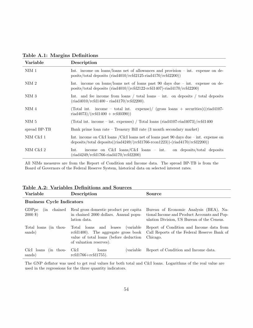
Table A.1: Margins Definitions
Variable Description
NIM 1 Int. income on loans/loans net of allowances and provision – int. expense on de-posits/total deposits (riad4010/rcfd2125-riad4170/rcfd2200))
NIM 2 Int. income on loans/loans net of loans past 90 days due – int. expense on de-posits/total deposits (riad4010/(rcfd2122-rcfd1407)-riad4170/rcfd2200)
NIM 3 Int. and fee income from loans / total loans – int. on deposits / total deposits(riad4010/rcfd1400 - riad4170/rcfd2200).
NIM 4 (Total int. income – total int. expense)/ (gross loans + securities)((riad4107-riad4073)/(rcfd1400 + rcfd0390))
NIM 5 (Total int. income – int. expenses) / Total loans (riad4107-riad4073)/rcfd1400
spread BP-TB Bank prime loan rate – Treasury Bill rate (3 month secondary market)
NIM C&I 1 Int. income on C&I loans /C&I loans net of loans past 90 days due – int. expense ondeposits/total deposits((riad4249/(rcfd1766-rcon1223))-(riad4170/rcfd2200))
NIM C&I 2 Int. income on C&I loans/C&I loans – int. on deposits/total deposits(riad4249/rcfd1766-riad4170/rcfd2200)
All NIMs measures are from the Report of Condition and Income data. The spread BP-TB is from theBoard of Governors of the Federal Reserve System, historical data on selected interest rates.
Table A.2: Variables Definitions and SourcesVariable Description Source
Business Cycle Indicators
GDPpc (in chained2000 $)
Real gross domestic product per capitain chained 2000 dollars. Annual popu-lation data.
Bureau of Economic Analysis (BEA), Na-tional Income and Product Accounts and Pop-ulation Division, US Bureau of the Census.
Total loans (in thou-sands)
Total loans and leases (variablercfd1400). The aggregate gross bookvalue of total loans (before deductionof valuation reserves).
Report of Condition and Income data fromCall Reports of the Federal Reserve Bank ofChicago.
C&I loans (in thou-sands)
C&I loans (variablercfd1766+rcfd1755).
Report of Condition and Income data.
The GNP deflator was used to get real values for both total and C&I loans. Logarithms of the real value areused in the regressions for the three quantity indicators.
54
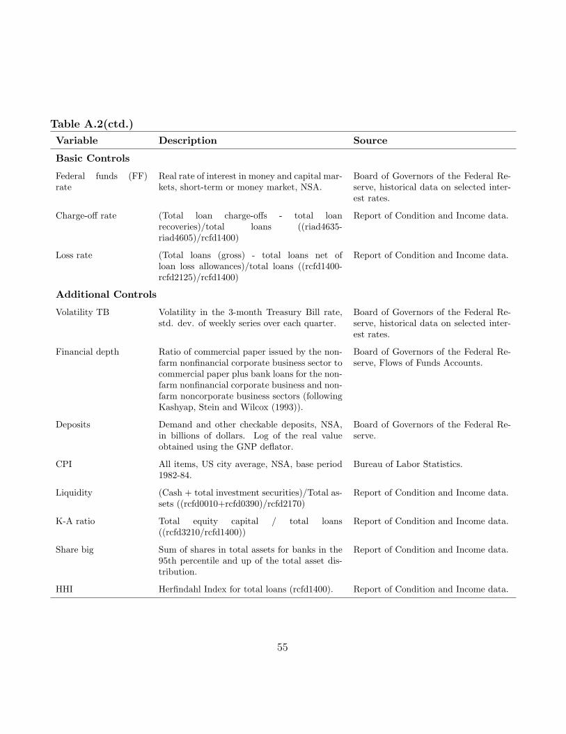
Table A.2(ctd.)
Variable Description Source
Basic Controls
Federal funds (FF)rate
Real rate of interest in money and capital mar-kets, short-term or money market, NSA.
Board of Governors of the Federal Re-serve, historical data on selected inter-est rates.
Charge-off rate (Total loan charge-offs - total loanrecoveries)/total loans ((riad4635-riad4605)/rcfd1400)
Report of Condition and Income data.
Loss rate (Total loans (gross) - total loans net ofloan loss allowances)/total loans ((rcfd1400-rcfd2125)/rcfd1400)
Report of Condition and Income data.
Additional Controls
Volatility TB Volatility in the 3-month Treasury Bill rate,std. dev. of weekly series over each quarter.
Board of Governors of the Federal Re-serve, historical data on selected inter-est rates.
Financial depth Ratio of commercial paper issued by the non-farm nonfinancial corporate business sector tocommercial paper plus bank loans for the non-farm nonfinancial corporate business and non-farm noncorporate business sectors (followingKashyap, Stein and Wilcox (1993)).
Board of Governors of the Federal Re-serve, Flows of Funds Accounts.
Deposits Demand and other checkable deposits, NSA,in billions of dollars. Log of the real valueobtained using the GNP deflator.
Board of Governors of the Federal Re-serve.
CPI All items, US city average, NSA, base period1982-84.
Bureau of Labor Statistics.
Liquidity (Cash + total investment securities)/Total as-sets ((rcfd0010+rcfd0390)/rcfd2170)
Report of Condition and Income data.
K-A ratio Total equity capital / total loans((rcfd3210/rcfd1400))
Report of Condition and Income data.
Share big Sum of shares in total assets for banks in the95th percentile and up of the total asset dis-tribution.
Report of Condition and Income data.
HHI Herfindahl Index for total loans (rcfd1400). Report of Condition and Income data.
55
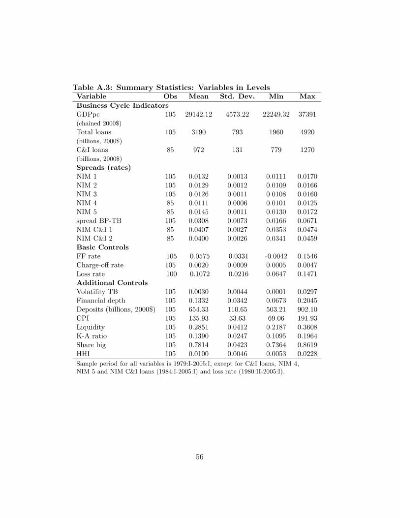
Table A.3: Summary Statistics: Variables in LevelsVariable Obs Mean Std. Dev. Min MaxBusiness Cycle IndicatorsGDPpc 105 29142.12 4573.22 22249.32 37391(chained 2000$)Total loans 105 3190 793 1960 4920(billions, 2000$)C&I loans 85 972 131 779 1270(billions, 2000$)Spreads (rates)NIM 1 105 0.0132 0.0013 0.0111 0.0170NIM 2 105 0.0129 0.0012 0.0109 0.0166NIM 3 105 0.0126 0.0011 0.0108 0.0160NIM 4 85 0.0111 0.0006 0.0101 0.0125NIM 5 85 0.0145 0.0011 0.0130 0.0172spread BP-TB 105 0.0308 0.0073 0.0166 0.0671NIM C&I 1 85 0.0407 0.0027 0.0353 0.0474NIM C&I 2 85 0.0400 0.0026 0.0341 0.0459Basic ControlsFF rate 105 0.0575 0.0331 -0.0042 0.1546Charge-off rate 105 0.0020 0.0009 0.0005 0.0047Loss rate 100 0.1072 0.0216 0.0647 0.1471Additional ControlsVolatility TB 105 0.0030 0.0044 0.0001 0.0297Financial depth 105 0.1332 0.0342 0.0673 0.2045Deposits (billions, 2000$) 105 654.33 110.65 503.21 902.10CPI 105 135.93 33.63 69.06 191.93Liquidity 105 0.2851 0.0412 0.2187 0.3608K-A ratio 105 0.1390 0.0247 0.1095 0.1964Share big 105 0.7814 0.0423 0.7364 0.8619HHI 105 0.0100 0.0046 0.0053 0.0228Sample period for all variables is 1979:I-2005:I, except for C&I loans, NIM 4,NIM 5 and NIM C&I loans (1984:I-2005:I) and loss rate (1980:II-2005:I).
56
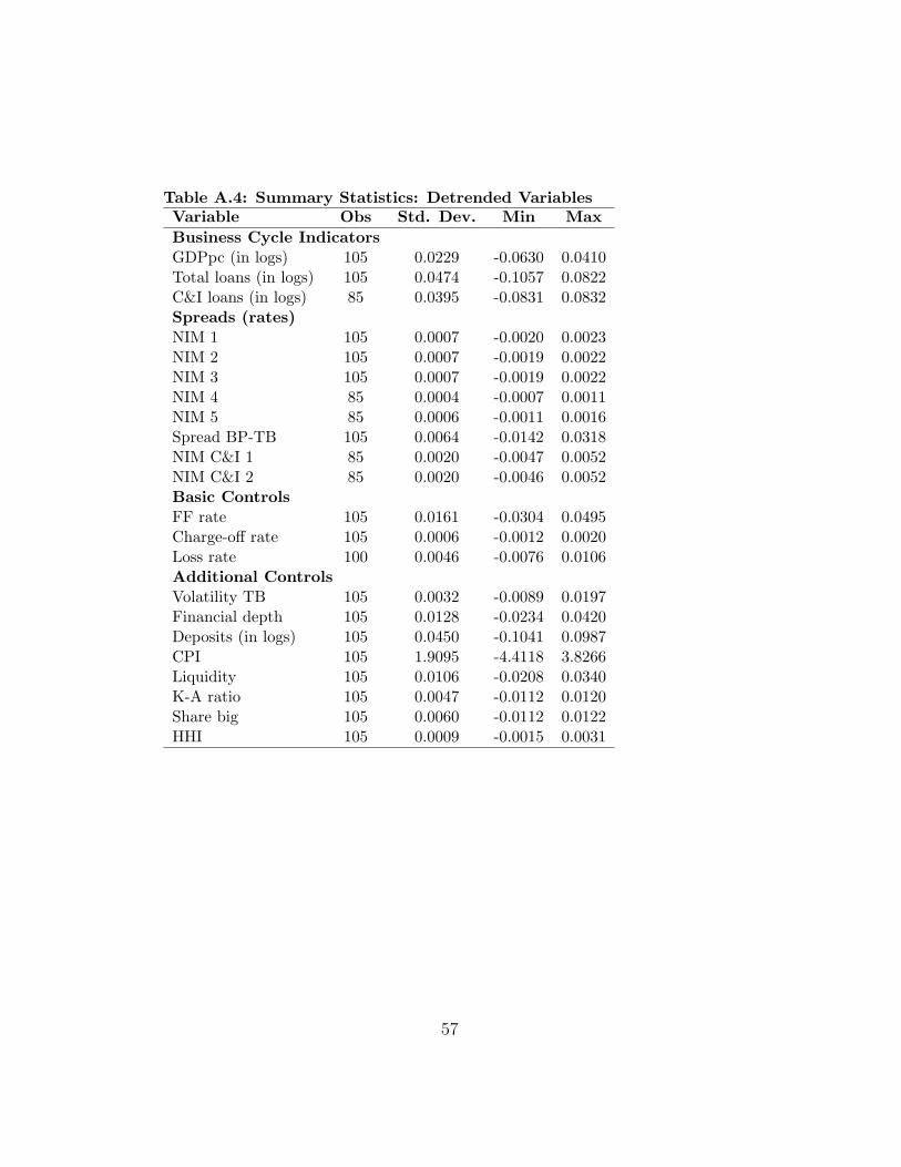
Table A.4: Summary Statistics: Detrended VariablesVariable Obs Std. Dev. Min MaxBusiness Cycle IndicatorsGDPpc (in logs) 105 0.0229 -0.0630 0.0410Total loans (in logs) 105 0.0474 -0.1057 0.0822C&I loans (in logs) 85 0.0395 -0.0831 0.0832Spreads (rates)NIM 1 105 0.0007 -0.0020 0.0023NIM 2 105 0.0007 -0.0019 0.0022NIM 3 105 0.0007 -0.0019 0.0022NIM 4 85 0.0004 -0.0007 0.0011NIM 5 85 0.0006 -0.0011 0.0016Spread BP-TB 105 0.0064 -0.0142 0.0318NIM C&I 1 85 0.0020 -0.0047 0.0052NIM C&I 2 85 0.0020 -0.0046 0.0052Basic ControlsFF rate 105 0.0161 -0.0304 0.0495Charge-off rate 105 0.0006 -0.0012 0.0020Loss rate 100 0.0046 -0.0076 0.0106Additional ControlsVolatility TB 105 0.0032 -0.0089 0.0197Financial depth 105 0.0128 -0.0234 0.0420Deposits (in logs) 105 0.0450 -0.1041 0.0987CPI 105 1.9095 -4.4118 3.8266Liquidity 105 0.0106 -0.0208 0.0340K-A ratio 105 0.0047 -0.0112 0.0120Share big 105 0.0060 -0.0112 0.0122HHI 105 0.0009 -0.0015 0.0031
57

Table A.5: Cyclicality of VariablesGDPpc Total Loans C&I Loans
Macroeconomic DeterminantsFF rate 0.2176 0.2588 0.5317
(0.026) (0.008) (0.000)FF ratet−1 0.0965 0.2367 0.5868
(0.330) (0.016) (0.000)Liquidity*Fed funds rate 0.2212 0.2566 0.1924
(0.023) (0.008) (0.078)HHI*Fed funds rate 0.2554 0.2904 0.3601
(0.009) (0.003) (0.001)Charge-off ratet−1 -0.2177 -0.1284 -0.0145
(0.026) (0.194) (0.896)Volatility TB -0.0745 0.0218 0.0915
(0.450) (0.825) (0.405)Volatility TBt−1 -0.1395 -0.0314 0.0816
(0.158) (0.752) (0.458)Financial deptht−1 -0.0019 0.1709 0.439
(0.985) (0.083) (0.000)Deposits 0.1134 -0.1152 -0.3084
(0.249) (0.242) (0.004)CPI -0.7221 -0.6831 -0.3992
(0.000) (0.000) (0.000)Bank-Level DeterminantsLiquidity -0.228 -0.489 -0.4609
(0.019) (0.000) (0.000)K-A ratio -0.2365 -0.4764 -0.3917
(0.015) (0.000) (0.000)Share big 0.6675 0.8034 0.6978
(0.000) (0.000) (0.000)Values shown are correlation coefficients of each variable with each cycle indicator.Significance levels in parentheses.
58
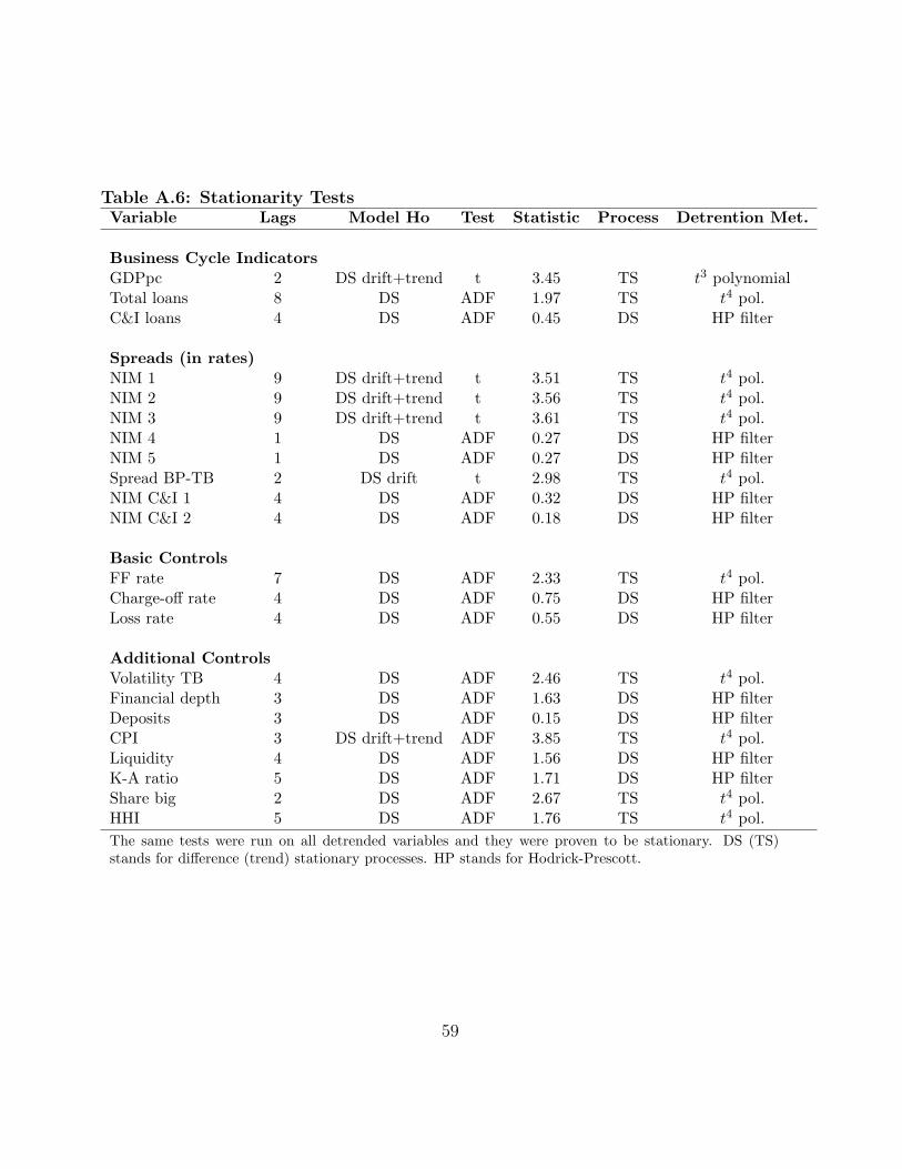
Table A.6: Stationarity TestsVariable Lags Model Ho Test Statistic Process Detrention Met.
Business Cycle IndicatorsGDPpc 2 DS drift+trend t 3.45 TS t3 polynomialTotal loans 8 DS ADF 1.97 TS t4 pol.C&I loans 4 DS ADF 0.45 DS HP filter
Spreads (in rates)NIM 1 9 DS drift+trend t 3.51 TS t4 pol.NIM 2 9 DS drift+trend t 3.56 TS t4 pol.NIM 3 9 DS drift+trend t 3.61 TS t4 pol.NIM 4 1 DS ADF 0.27 DS HP filterNIM 5 1 DS ADF 0.27 DS HP filterSpread BP-TB 2 DS drift t 2.98 TS t4 pol.NIM C&I 1 4 DS ADF 0.32 DS HP filterNIM C&I 2 4 DS ADF 0.18 DS HP filter
Basic ControlsFF rate 7 DS ADF 2.33 TS t4 pol.Charge-off rate 4 DS ADF 0.75 DS HP filterLoss rate 4 DS ADF 0.55 DS HP filter
Additional ControlsVolatility TB 4 DS ADF 2.46 TS t4 pol.Financial depth 3 DS ADF 1.63 DS HP filterDeposits 3 DS ADF 0.15 DS HP filterCPI 3 DS drift+trend ADF 3.85 TS t4 pol.Liquidity 4 DS ADF 1.56 DS HP filterK-A ratio 5 DS ADF 1.71 DS HP filterShare big 2 DS ADF 2.67 TS t4 pol.HHI 5 DS ADF 1.76 TS t4 pol.The same tests were run on all detrended variables and they were proven to be stationary. DS (TS)stands for difference (trend) stationary processes. HP stands for Hodrick-Prescott.
59
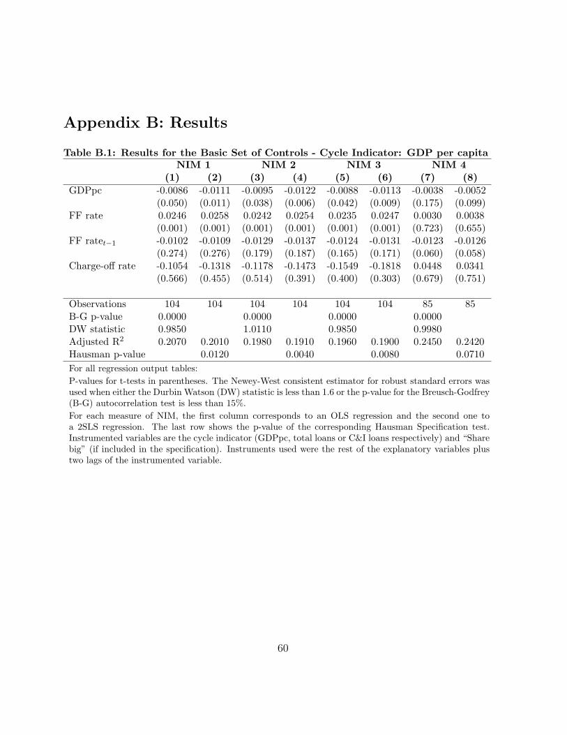
Appendix B: Results
Table B.1: Results for the Basic Set of Controls - Cycle Indicator: GDP per capitaNIM 1 NIM 2 NIM 3 NIM 4
(1) (2) (3) (4) (5) (6) (7) (8)GDPpc -0.0086 -0.0111 -0.0095 -0.0122 -0.0088 -0.0113 -0.0038 -0.0052
(0.050) (0.011) (0.038) (0.006) (0.042) (0.009) (0.175) (0.099)FF rate 0.0246 0.0258 0.0242 0.0254 0.0235 0.0247 0.0030 0.0038
(0.001) (0.001) (0.001) (0.001) (0.001) (0.001) (0.723) (0.655)FF ratet−1 -0.0102 -0.0109 -0.0129 -0.0137 -0.0124 -0.0131 -0.0123 -0.0126
(0.274) (0.276) (0.179) (0.187) (0.165) (0.171) (0.060) (0.058)Charge-off rate -0.1054 -0.1318 -0.1178 -0.1473 -0.1549 -0.1818 0.0448 0.0341
(0.566) (0.455) (0.514) (0.391) (0.400) (0.303) (0.679) (0.751)
Observations 104 104 104 104 104 104 85 85B-G p-value 0.0000 0.0000 0.0000 0.0000DW statistic 0.9850 1.0110 0.9850 0.9980Adjusted R2 0.2070 0.2010 0.1980 0.1910 0.1960 0.1900 0.2450 0.2420Hausman p-value 0.0120 0.0040 0.0080 0.0710For all regression output tables:P-values for t-tests in parentheses. The Newey-West consistent estimator for robust standard errors wasused when either the Durbin Watson (DW) statistic is less than 1.6 or the p-value for the Breusch-Godfrey(B-G) autocorrelation test is less than 15%.For each measure of NIM, the first column corresponds to an OLS regression and the second one toa 2SLS regression. The last row shows the p-value of the corresponding Hausman Specification test.Instrumented variables are the cycle indicator (GDPpc, total loans or C&I loans respectively) and “Sharebig” (if included in the specification). Instruments used were the rest of the explanatory variables plustwo lags of the instrumented variable.
60
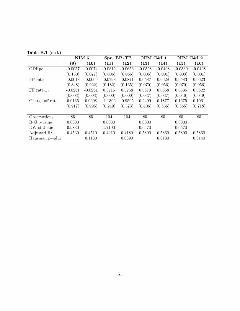
Table B.1 (ctd.)NIM 5 Spr. BP/TB NIM C&I 1 NIM C&I 2
(9) (10) (11) (12) (13) (14) (15) (16)GDPpc -0.0057 -0.0074 -0.0812 -0.0653 -0.0328 -0.0408 -0.0330 -0.0408
(0.130) (0.077) (0.006) (0.066) (0.005) (0.001) (0.003) (0.001)FF rate -0.0018 -0.0009 -0.0798 -0.0871 0.0587 0.0628 0.0583 0.0623
(0.848) (0.922) (0.182) (0.165) (0.070) (0.056) (0.070) (0.056)FF ratet−1 -0.0251 -0.0254 0.3216 0.3258 0.0573 0.0558 0.0536 0.0522
(0.003) (0.003) (0.000) (0.000) (0.037) (0.037) (0.046) (0.049)Charge-off rate 0.0135 0.0008 -1.1306 -0.9595 0.2499 0.1877 0.1675 0.1061
(0.917) (0.995) (0.249) (0.373) (0.406) (0.536) (0.565) (0.718)
Observations 85 85 104 104 85 85 85 85B-G p-value 0.0000 0.0030 0.0000 0.0000DW statistic 0.9830 1.7190 0.6470 0.6570Adjusted R2 0.4530 0.4510 0.4210 0.4180 0.5890 0.5860 0.5890 0.5860Hausman p-value 0.1130 0.0390 0.0130 0.0140
61
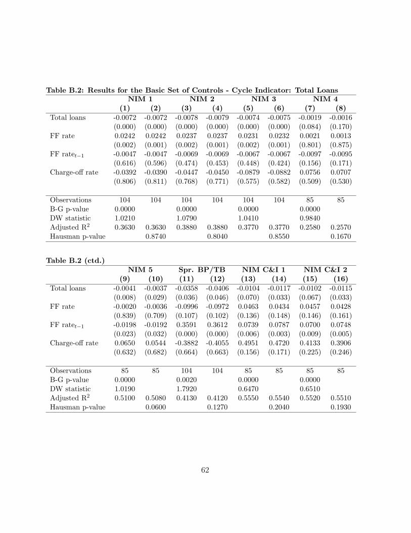
Table B.2: Results for the Basic Set of Controls - Cycle Indicator: Total LoansNIM 1 NIM 2 NIM 3 NIM 4
(1) (2) (3) (4) (5) (6) (7) (8)Total loans -0.0072 -0.0072 -0.0078 -0.0079 -0.0074 -0.0075 -0.0019 -0.0016
(0.000) (0.000) (0.000) (0.000) (0.000) (0.000) (0.084) (0.170)FF rate 0.0242 0.0242 0.0237 0.0237 0.0231 0.0232 0.0021 0.0013
(0.002) (0.001) (0.002) (0.001) (0.002) (0.001) (0.801) (0.875)FF ratet−1 -0.0047 -0.0047 -0.0069 -0.0069 -0.0067 -0.0067 -0.0097 -0.0095
(0.616) (0.596) (0.474) (0.453) (0.448) (0.424) (0.156) (0.171)Charge-off rate -0.0392 -0.0390 -0.0447 -0.0450 -0.0879 -0.0882 0.0756 0.0707
(0.806) (0.811) (0.768) (0.771) (0.575) (0.582) (0.509) (0.530)
Observations 104 104 104 104 104 104 85 85B-G p-value 0.0000 0.0000 0.0000 0.0000DW statistic 1.0210 1.0790 1.0410 0.9840Adjusted R2 0.3630 0.3630 0.3880 0.3880 0.3770 0.3770 0.2580 0.2570Hausman p-value 0.8740 0.8040 0.8550 0.1670
Table B.2 (ctd.)NIM 5 Spr. BP/TB NIM C&I 1 NIM C&I 2
(9) (10) (11) (12) (13) (14) (15) (16)Total loans -0.0041 -0.0037 -0.0358 -0.0406 -0.0104 -0.0117 -0.0102 -0.0115
(0.008) (0.029) (0.036) (0.046) (0.070) (0.033) (0.067) (0.033)FF rate -0.0020 -0.0036 -0.0996 -0.0972 0.0463 0.0434 0.0457 0.0428
(0.839) (0.709) (0.107) (0.102) (0.136) (0.148) (0.146) (0.161)FF ratet−1 -0.0198 -0.0192 0.3591 0.3612 0.0739 0.0787 0.0700 0.0748
(0.023) (0.032) (0.000) (0.000) (0.006) (0.003) (0.009) (0.005)Charge-off rate 0.0650 0.0544 -0.3882 -0.4055 0.4951 0.4720 0.4133 0.3906
(0.632) (0.682) (0.664) (0.663) (0.156) (0.171) (0.225) (0.246)
Observations 85 85 104 104 85 85 85 85B-G p-value 0.0000 0.0020 0.0000 0.0000DW statistic 1.0190 1.7920 0.6470 0.6510Adjusted R2 0.5100 0.5080 0.4130 0.4120 0.5550 0.5540 0.5520 0.5510Hausman p-value 0.0600 0.1270 0.2040 0.1930
62
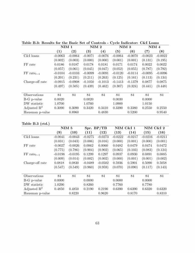
Table B.3: Results for the Basic Set of Controls - Cycle Indicator: C&I LoansNIM 1 NIM 2 NIM 3 NIM 4
(1) (2) (3) (4) (5) (6) (7) (8)C&I loans -0.0063 -0.0064 -0.0071 -0.0076 -0.0064 -0.0070 -0.0023 -0.0022
(0.002) (0.003) (0.000) (0.000) (0.001) (0.001) (0.131) (0.195)FF rate 0.0186 0.0187 0.0178 0.0181 0.0171 0.0174 0.0022 0.0022
(0.057) (0.061) (0.045) (0.047) (0.052) (0.055) (0.787) (0.792)FF ratet−1 -0.0104 -0.0103 -0.0099 -0.0091 -0.0120 -0.0114 -0.0095 -0.0096
(0.201) (0.231) (0.211) (0.263) (0.125) (0.161) (0.113) (0.134)Charge-off rate -0.0915 -0.0908 -0.1050 -0.1013 -0.1413 -0.1379 0.0877 0.0875
(0.497) (0.505) (0.439) (0.462) (0.307) (0.324) (0.441) (0.448)
Observations 84 84 84 84 84 84 84 84B-G p-value 0.0020 0.0020 0.0030 0.0000DW statistic 1.0700 1.0760 1.0900 1.0150Adjusted R2 0.3090 0.3090 0.3420 0.3410 0.3390 0.3380 0.2550 0.2550Hausman p-value 0.8960 0.4830 0.5200 0.9540
Table B.3 (ctd.)NIM 5 Spr. BP/TB NIM C&I 1 NIM C&I 2
(9) (10) (11) (12) (13) (14) (15) (16)C&I loans -0.0041 -0.0043 -0.0275 -0.0273 -0.0222 -0.0217 -0.0216 -0.0211
(0.031) (0.043) (0.006) (0.016) (0.000) (0.001) (0.000) (0.001)FF rate -0.0027 -0.0026 0.0062 0.0060 0.0482 0.0479 0.0474 0.0472
(0.775) (0.786) (0.904) (0.902) (0.065) (0.103) (0.083) (0.124)FF ratet−1 -0.0198 -0.0195 0.1299 0.1297 0.0937 0.0930 0.0891 0.0885
(0.009) (0.014) (0.002) (0.002) (0.000) (0.001) (0.001) (0.002)Charge-off rate 0.0818 0.0830 -0.0489 -0.0502 0.5936 0.5901 0.5090 0.5058
(0.547) (0.549) (0.960) (0.959) (0.070) (0.090) (0.117) (0.143)
Observations 84 84 84 84 84 84 84 84B-G p-value 0.0000 0.0000 0.0000 0.0000DW statistic 1.0290 0.8260 0.7760 0.7780Adjusted R2 0.4850 0.4850 0.2190 0.2190 0.6390 0.6390 0.6320 0.6320Hausman p-value 0.8220 0.9620 0.8170 0.8310
63

Table B.4: Explaining the Countercyclicality - Cycle Indicator: GDP per capitaNIM 1 NIM 2 NIM 3 NIM 4
(1) (2) (3) (4) (5) (6) (7) (8)Macroeconomic DeterminantsGDPpc 0.0019 -0.0038 0.0023 -0.0040 0.0027 -0.0031 0.0000 -0.0043
(0.634) (0.443) (0.588) (0.457) (0.454) (0.504) (1.000) (0.538)FF rate 0.0253 0.0290 0.0244 0.0292 0.0239 0.0286 0.0109 0.0127
(0.000) (0.001) (0.000) (0.000) (0.000) (0.000) (0.180) (0.121)FF ratet−1 0.0096 0.0099 0.0075 0.0083 0.0079 0.0089 -0.0096 -0.0091
(0.244) (0.274) (0.357) (0.352) (0.303) (0.286) (0.155) (0.184)Liquidity*FF rate 0.2909 0.2939 0.3132 0.3012 0.3888 0.3688 0.4507 0.4394
(0.290) (0.351) (0.268) (0.347) (0.134) (0.218) (0.324) (0.407)HHI*FF rate -0.7694 0.8767 0.5668 2.4953 -0.3470 1.4671 -0.0586 1.3563
(0.879) (0.860) (0.907) (0.599) (0.940) (0.747) (0.990) (0.775)Charge-off rate 0.1307 0.0991 0.1303 0.1008 0.1225 0.0989 0.0656 0.0354
(0.424) (0.546) (0.413) (0.522) (0.409) (0.501) (0.502) (0.709)Volatility TB 0.0201 0.0209 0.0126 0.0140 0.0161 0.0178 0.0572 0.0533
(0.252) (0.325) (0.514) (0.553) (0.311) (0.376) (0.037) (0.043)Volatility TBt−1 0.0232 0.0217 0.0182 0.0179 0.0200 0.0205 0.0726 0.0747
(0.135) (0.207) (0.276) (0.319) (0.186) (0.216) (0.007) (0.018)Financial depth -0.0087 -0.0085 -0.0081 -0.0079 -0.0070 -0.0068 -0.0070 -0.0067
(0.098) (0.106) (0.107) (0.116) (0.139) (0.150) (0.036) (0.057)Deposits 0.0026 0.0021 0.0027 0.0022 0.0032 0.0027 -0.0022 -0.0026
(0.207) (0.291) (0.173) (0.262) (0.087) (0.134) (0.072) (0.065)CPI 0.0000 -0.0001 0.0000 -0.0001 0.0000 -0.0001 -0.0001 -0.0001
(0.860) (0.392) (0.961) (0.296) (0.902) (0.263) (0.418) (0.203)Bank-Level DeterminantsLiquidity 0.0208 0.0222 0.0181 0.0194 0.0176 0.0188 0.0015 0.0025
(0.001) (0.000) (0.007) (0.001) (0.003) (0.000) (0.841) (0.766)K-A ratio 0.0354 0.0345 0.0390 0.0377 0.0402 0.0390 0.0337 0.0320
(0.075) (0.105) (0.038) (0.062) (0.030) (0.050) (0.003) (0.006)Share big -0.0427 -0.0456 -0.0499 -0.0575 -0.0487 -0.0580 -0.0256 -0.0280
(0.005) (0.075) (0.001) (0.017) (0.000) (0.012) (0.023) (0.135)
Observations 104 104 104 104 104 104 85 85B-G p-value 0.0020 0.0010 0.0040 0.0960DW statistic 1.3300 1.3170 1.3670 1.5320Adjusted R2 0.5860 0.5820 0.5820 0.5760 0.6110 0.6060 0.4020 0.3990Hausman p-value 0.2160 0.1490 0.1900 0.4090
64
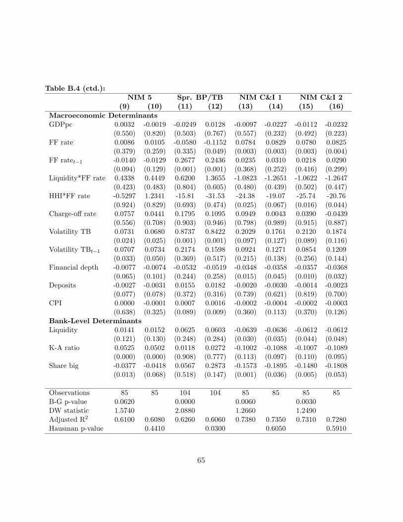
Table B.4 (ctd.):NIM 5 Spr. BP/TB NIM C&I 1 NIM C&I 2
(9) (10) (11) (12) (13) (14) (15) (16)Macroeconomic DeterminantsGDPpc 0.0032 -0.0019 -0.0249 0.0128 -0.0097 -0.0227 -0.0112 -0.0232
(0.550) (0.820) (0.503) (0.767) (0.557) (0.232) (0.492) (0.223)FF rate 0.0086 0.0105 -0.0580 -0.1152 0.0784 0.0829 0.0780 0.0825
(0.379) (0.259) (0.335) (0.049) (0.003) (0.003) (0.003) (0.004)FF ratet−1 -0.0140 -0.0129 0.2677 0.2436 0.0235 0.0310 0.0218 0.0290
(0.094) (0.129) (0.001) (0.001) (0.368) (0.252) (0.416) (0.299)Liquidity*FF rate 0.4338 0.4449 0.6200 1.3655 -1.0823 -1.2651 -1.0622 -1.2647
(0.423) (0.483) (0.804) (0.605) (0.480) (0.439) (0.502) (0.447)HHI*FF rate -0.5297 1.2341 -15.81 -31.53 -24.38 -19.07 -25.74 -20.76
(0.924) (0.829) (0.693) (0.474) (0.025) (0.067) (0.016) (0.044)Charge-off rate 0.0757 0.0441 0.1795 0.1095 0.0949 0.0043 0.0390 -0.0439
(0.556) (0.708) (0.903) (0.946) (0.798) (0.989) (0.915) (0.887)Volatility TB 0.0731 0.0680 0.8737 0.8422 0.2029 0.1761 0.2120 0.1874
(0.024) (0.025) (0.001) (0.001) (0.097) (0.127) (0.089) (0.116)Volatility TBt−1 0.0707 0.0734 0.2174 0.1598 0.0924 0.1271 0.0854 0.1209
(0.033) (0.050) (0.369) (0.517) (0.215) (0.138) (0.256) (0.144)Financial depth -0.0077 -0.0074 -0.0532 -0.0519 -0.0348 -0.0358 -0.0357 -0.0368
(0.065) (0.101) (0.244) (0.258) (0.015) (0.045) (0.010) (0.032)Deposits -0.0027 -0.0031 0.0155 0.0182 -0.0020 -0.0030 -0.0014 -0.0023
(0.077) (0.078) (0.372) (0.316) (0.739) (0.621) (0.819) (0.700)CPI 0.0000 -0.0001 0.0007 0.0016 -0.0002 -0.0004 -0.0002 -0.0003
(0.638) (0.325) (0.089) (0.009) (0.360) (0.113) (0.370) (0.126)Bank-Level DeterminantsLiquidity 0.0141 0.0152 0.0625 0.0603 -0.0639 -0.0636 -0.0612 -0.0612
(0.121) (0.130) (0.248) (0.284) (0.030) (0.035) (0.044) (0.048)K-A ratio 0.0525 0.0502 0.0118 0.0272 -0.1002 -0.1088 -0.1007 -0.1089
(0.000) (0.000) (0.908) (0.777) (0.113) (0.097) (0.110) (0.095)Share big -0.0377 -0.0418 0.0567 0.2873 -0.1573 -0.1895 -0.1480 -0.1808
(0.013) (0.068) (0.518) (0.147) (0.001) (0.036) (0.005) (0.053)
Observations 85 85 104 104 85 85 85 85B-G p-value 0.0620 0.0000 0.0060 0.0030DW statistic 1.5740 2.0880 1.2660 1.2490Adjusted R2 0.6100 0.6080 0.6260 0.6060 0.7380 0.7350 0.7310 0.7280Hausman p-value 0.4410 0.0300 0.6050 0.5910
65
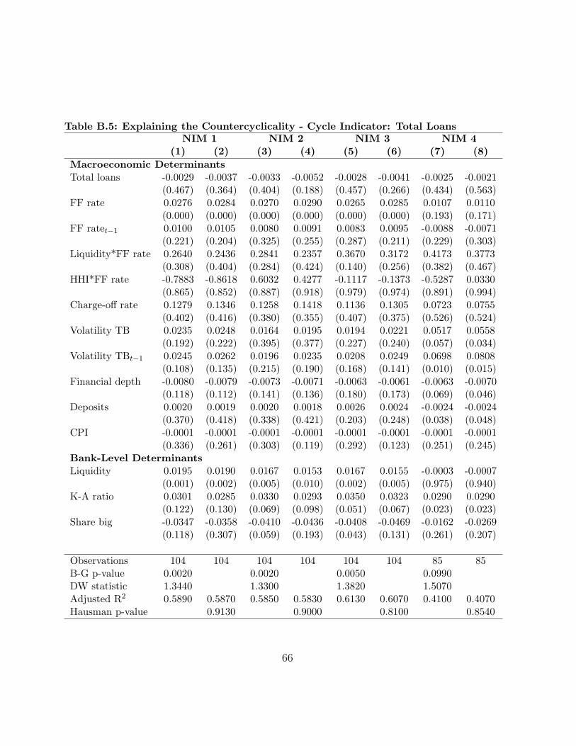
Table B.5: Explaining the Countercyclicality - Cycle Indicator: Total LoansNIM 1 NIM 2 NIM 3 NIM 4
(1) (2) (3) (4) (5) (6) (7) (8)Macroeconomic DeterminantsTotal loans -0.0029 -0.0037 -0.0033 -0.0052 -0.0028 -0.0041 -0.0025 -0.0021
(0.467) (0.364) (0.404) (0.188) (0.457) (0.266) (0.434) (0.563)FF rate 0.0276 0.0284 0.0270 0.0290 0.0265 0.0285 0.0107 0.0110
(0.000) (0.000) (0.000) (0.000) (0.000) (0.000) (0.193) (0.171)FF ratet−1 0.0100 0.0105 0.0080 0.0091 0.0083 0.0095 -0.0088 -0.0071
(0.221) (0.204) (0.325) (0.255) (0.287) (0.211) (0.229) (0.303)Liquidity*FF rate 0.2640 0.2436 0.2841 0.2357 0.3670 0.3172 0.4173 0.3773
(0.308) (0.404) (0.284) (0.424) (0.140) (0.256) (0.382) (0.467)HHI*FF rate -0.7883 -0.8618 0.6032 0.4277 -0.1117 -0.1373 -0.5287 0.0330
(0.865) (0.852) (0.887) (0.918) (0.979) (0.974) (0.891) (0.994)Charge-off rate 0.1279 0.1346 0.1258 0.1418 0.1136 0.1305 0.0723 0.0755
(0.402) (0.416) (0.380) (0.355) (0.407) (0.375) (0.526) (0.524)Volatility TB 0.0235 0.0248 0.0164 0.0195 0.0194 0.0221 0.0517 0.0558
(0.192) (0.222) (0.395) (0.377) (0.227) (0.240) (0.057) (0.034)Volatility TBt−1 0.0245 0.0262 0.0196 0.0235 0.0208 0.0249 0.0698 0.0808
(0.108) (0.135) (0.215) (0.190) (0.168) (0.141) (0.010) (0.015)Financial depth -0.0080 -0.0079 -0.0073 -0.0071 -0.0063 -0.0061 -0.0063 -0.0070
(0.118) (0.112) (0.141) (0.136) (0.180) (0.173) (0.069) (0.046)Deposits 0.0020 0.0019 0.0020 0.0018 0.0026 0.0024 -0.0024 -0.0024
(0.370) (0.418) (0.338) (0.421) (0.203) (0.248) (0.038) (0.048)CPI -0.0001 -0.0001 -0.0001 -0.0001 -0.0001 -0.0001 -0.0001 -0.0001
(0.336) (0.261) (0.303) (0.119) (0.292) (0.123) (0.251) (0.245)Bank-Level DeterminantsLiquidity 0.0195 0.0190 0.0167 0.0153 0.0167 0.0155 -0.0003 -0.0007
(0.001) (0.002) (0.005) (0.010) (0.002) (0.005) (0.975) (0.940)K-A ratio 0.0301 0.0285 0.0330 0.0293 0.0350 0.0323 0.0290 0.0290
(0.122) (0.130) (0.069) (0.098) (0.051) (0.067) (0.023) (0.023)Share big -0.0347 -0.0358 -0.0410 -0.0436 -0.0408 -0.0469 -0.0162 -0.0269
(0.118) (0.307) (0.059) (0.193) (0.043) (0.131) (0.261) (0.207)
Observations 104 104 104 104 104 104 85 85B-G p-value 0.0020 0.0020 0.0050 0.0990DW statistic 1.3440 1.3300 1.3820 1.5070Adjusted R2 0.5890 0.5870 0.5850 0.5830 0.6130 0.6070 0.4100 0.4070Hausman p-value 0.9130 0.9000 0.8100 0.8540
66
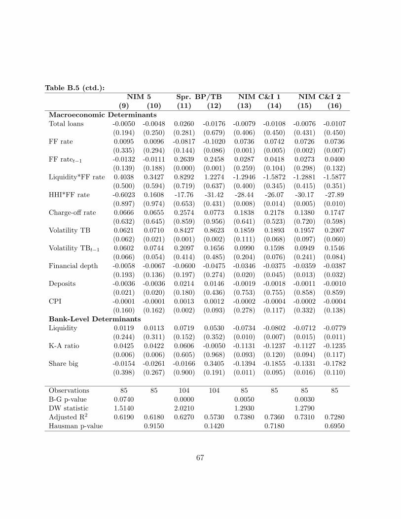
Table B.5 (ctd.):NIM 5 Spr. BP/TB NIM C&I 1 NIM C&I 2
(9) (10) (11) (12) (13) (14) (15) (16)Macroeconomic DeterminantsTotal loans -0.0050 -0.0048 0.0260 -0.0176 -0.0079 -0.0108 -0.0076 -0.0107
(0.194) (0.250) (0.281) (0.679) (0.406) (0.450) (0.431) (0.450)FF rate 0.0095 0.0096 -0.0817 -0.1020 0.0736 0.0742 0.0726 0.0736
(0.335) (0.294) (0.144) (0.086) (0.001) (0.005) (0.002) (0.007)FF ratet−1 -0.0132 -0.0111 0.2639 0.2458 0.0287 0.0418 0.0273 0.0400
(0.139) (0.188) (0.000) (0.001) (0.259) (0.104) (0.298) (0.132)Liquidity*FF rate 0.4038 0.3427 0.8292 1.2274 -1.2946 -1.5872 -1.2881 -1.5877
(0.500) (0.594) (0.719) (0.637) (0.400) (0.345) (0.415) (0.351)HHI*FF rate -0.6023 0.1608 -17.76 -31.42 -28.44 -26.07 -30.17 -27.89
(0.897) (0.974) (0.653) (0.431) (0.008) (0.014) (0.005) (0.010)Charge-off rate 0.0666 0.0655 0.2574 0.0773 0.1838 0.2178 0.1380 0.1747
(0.632) (0.645) (0.859) (0.956) (0.641) (0.523) (0.720) (0.598)Volatility TB 0.0621 0.0710 0.8427 0.8623 0.1859 0.1893 0.1957 0.2007
(0.062) (0.021) (0.001) (0.002) (0.111) (0.068) (0.097) (0.060)Volatility TBt−1 0.0602 0.0744 0.2097 0.1656 0.0990 0.1598 0.0949 0.1546
(0.066) (0.054) (0.414) (0.485) (0.204) (0.076) (0.241) (0.084)Financial depth -0.0058 -0.0067 -0.0600 -0.0475 -0.0346 -0.0375 -0.0359 -0.0387
(0.193) (0.136) (0.197) (0.274) (0.020) (0.045) (0.013) (0.032)Deposits -0.0036 -0.0036 0.0214 0.0146 -0.0019 -0.0018 -0.0011 -0.0010
(0.021) (0.020) (0.180) (0.436) (0.753) (0.755) (0.858) (0.859)CPI -0.0001 -0.0001 0.0013 0.0012 -0.0002 -0.0004 -0.0002 -0.0004
(0.160) (0.162) (0.002) (0.093) (0.278) (0.117) (0.332) (0.138)Bank-Level DeterminantsLiquidity 0.0119 0.0113 0.0719 0.0530 -0.0734 -0.0802 -0.0712 -0.0779
(0.244) (0.311) (0.152) (0.352) (0.010) (0.007) (0.015) (0.011)K-A ratio 0.0425 0.0422 0.0606 -0.0050 -0.1131 -0.1237 -0.1127 -0.1235
(0.006) (0.006) (0.605) (0.968) (0.093) (0.120) (0.094) (0.117)Share big -0.0154 -0.0261 -0.0166 0.3405 -0.1394 -0.1855 -0.1331 -0.1782
(0.398) (0.267) (0.900) (0.191) (0.011) (0.095) (0.016) (0.110)
Observations 85 85 104 104 85 85 85 85B-G p-value 0.0740 0.0000 0.0050 0.0030DW statistic 1.5140 2.0210 1.2930 1.2790Adjusted R2 0.6190 0.6180 0.6270 0.5730 0.7380 0.7360 0.7310 0.7280Hausman p-value 0.9150 0.1420 0.7180 0.6950
67

Table B.6: Explaining the Countercyclicality - Cycle Indicator: C&I LoansNIM 1 NIM 2 NIM 3 NIM 4
(1) (2) (3) (4) (5) (6) (7) (8)Macroeconomic DeterminantsC&I loans -0.0030 -0.0025 -0.0032 -0.0030 -0.0028 -0.0026 0.0001 -0.0002
(0.153) (0.322) (0.094) (0.197) (0.137) (0.257) (0.949) (0.909)FF rate 0.0282 0.0299 0.0283 0.0310 0.0276 0.0300 0.0107 0.0108
(0.018) (0.014) (0.011) (0.007) (0.012) (0.008) (0.189) (0.178)FF ratet−1 0.0020 0.0038 0.0028 0.0055 0.0012 0.0039 -0.0097 -0.0076
(0.864) (0.738) (0.796) (0.599) (0.910) (0.708) (0.154) (0.220)Liquidity*FF rate 0.6255 0.5444 0.8258 0.7100 0.7992 0.6910 0.5008 0.4683
(0.343) (0.465) (0.182) (0.305) (0.201) (0.323) (0.287) (0.368)HHI*FF rate -3.92 -3.45 -3.04 -2.41 -2.93 -2.33 -0.0044 0.3067
(0.461) (0.530) (0.552) (0.648) (0.566) (0.659) (0.999) (0.943)Charge-off rate 0.1126 0.1266 0.1144 0.1430 0.0938 0.1203 0.0555 0.0671
(0.483) (0.479) (0.438) (0.379) (0.521) (0.457) (0.641) (0.589)Volatility TB 0.0308 0.0354 0.0198 0.0259 0.0201 0.0254 0.0534 0.0506
(0.414) (0.369) (0.575) (0.476) (0.563) (0.479) (0.048) (0.059)Volatility TBt−1 0.0001 0.0156 -0.0104 0.0103 -0.0118 0.0079 0.0652 0.0738
(0.998) (0.762) (0.791) (0.826) (0.760) (0.867) (0.036) (0.056)Financial depth -0.0015 -0.0028 0.0000 -0.0011 -0.0001 -0.0012 -0.0073 -0.0075
(0.724) (0.592) (0.995) (0.832) (0.974) (0.812) (0.023) (0.077)Deposits 0.0027 0.0029 0.0029 0.0031 0.0031 0.0033 -0.0022 -0.0021
(0.204) (0.199) (0.138) (0.125) (0.113) (0.103) (0.074) (0.107)CPI 0.0000 0.0000 0.0000 0.0000 0.0000 0.0000 0.0000 -0.0001
(0.900) (0.762) (0.815) (0.613) (0.928) (0.562) (0.406) (0.266)Bank-Level DeterminantsLiquidity 0.0186 0.0176 0.0183 0.0168 0.0173 0.0159 0.0020 0.0011
(0.119) (0.176) (0.094) (0.160) (0.112) (0.182) (0.793) (0.892)K-A ratio 0.0220 0.0206 0.0294 0.0276 0.0294 0.0276 0.0333 0.0324
(0.263) (0.328) (0.126) (0.174) (0.126) (0.173) (0.002) (0.004)Share big -0.0202 -0.0371 -0.0271 -0.0498 -0.0272 -0.0488 -0.0250 -0.0334
(0.228) (0.293) (0.076) (0.106) (0.070) (0.112) (0.046) (0.083)
Observations 84 84 84 84 84 84 84 84B-G p-value 0.0070 0.0140 0.0170 0.0980DW statistic 1.2610 1.3050 1.3120 1.5220Adjusted R2 0.3840 0.3830 0.4480 0.4440 0.4450 0.4410 0.3920 0.3890Hausman p-value 0.8940 0.6540 0.6720 0.7540
68

Table B.6 (ctd.):NIM 5 Spr. BP/TB NIM C&I 1 NIM C&I 2
(9) (10) (11) (12) (13) (14) (15) (16)Macroeconomic DeterminantsC&I loans -0.0006 -0.0014 0.0086 0.0049 -0.0180 -0.0171 -0.0164 -0.0158
(0.708) (0.468) (0.472) (0.761) (0.001) (0.030) (0.003) (0.050)FF rate 0.0098 0.0100 0.0224 0.0056 0.0764 0.0793 0.0750 0.0783
(0.318) (0.278) (0.667) (0.920) (0.000) (0.002) (0.000) (0.003)FF ratet−1 -0.0145 -0.0116 0.0817 0.0802 0.0377 0.0478 0.0353 0.0453
(0.092) (0.133) (0.114) (0.123) (0.090) (0.056) (0.131) (0.079)Liquidity*FF rate 0.5169 0.4811 -3.5101 -2.9754 -0.9632 -1.2067 -0.9629 -1.2076
(0.380) (0.447) (0.101) (0.166) (0.513) (0.426) (0.524) (0.433)HHI*FF rate 0.3285 0.6665 -26.57 -28.44 -27.95 -25.99 -29.62 -27.72
(0.946) (0.898) (0.153) (0.160) (0.003) (0.009) (0.004) (0.010)Charge-off rate 0.0535 0.0752 -0.6833 -0.7775 0.4013 0.4490 0.3315 0.3843
(0.723) (0.626) (0.518) (0.492) (0.306) (0.239) (0.398) (0.306)Volatility TB 0.0681 0.0631 0.6459 0.5810 0.1475 0.1454 0.1603 0.1587
(0.042) (0.040) (0.002) (0.005) (0.130) (0.089) (0.107) (0.074)Volatility TBt−1 0.0577 0.0669 0.2975 0.2229 0.0469 0.1043 0.0452 0.1015
(0.148) (0.149) (0.283) (0.426) (0.681) (0.337) (0.702) (0.362)Financial depth -0.0066 -0.0060 -0.0630 -0.0558 -0.0132 -0.0171 -0.0166 -0.0200
(0.108) (0.256) (0.049) (0.121) (0.391) (0.418) (0.274) (0.337)Deposits -0.0031 -0.0030 0.0021 0.0017 -0.0016 -0.0009 -0.0007 0.0000
(0.063) (0.082) (0.815) (0.844) (0.781) (0.888) (0.896) (0.994)CPI -0.0001 -0.0001 0.0007 0.0009 -0.0002 -0.0004 -0.0002 -0.0003
(0.425) (0.245) (0.017) (0.022) (0.108) (0.059) (0.161) (0.080)Bank-Level DeterminantsLiquidity 0.0157 0.0145 0.0490 0.0521 -0.0708 -0.0754 -0.0684 -0.0730
(0.095) (0.152) (0.248) (0.204) (0.002) (0.004) (0.005) (0.007)K-A ratio 0.0517 0.0508 -0.0602 -0.0548 -0.0944 -0.1003 -0.0950 -0.1007
(0.000) (0.000) (0.400) (0.437) (0.132) (0.128) (0.129) (0.125)Share big -0.0319 -0.0405 -0.0114 0.0795 -0.1234 -0.1827 -0.1197 -0.1781
(0.050) (0.064) (0.880) (0.431) (0.003) (0.015) (0.006) (0.023)
Observations 84 84 84 84 84 84 84 84B-G p-value 0.0550 0.0000 0.0010 0.0000DW statistic 1.5310 1.1610 1.3970 1.3610Adjusted R2 0.6050 0.6010 0.4650 0.4590 0.7760 0.7750 0.7620 0.7610Hausman p-value 0.6090 0.6110 0.8250 0.7950
69
Appendix C: Robustness Checks
A series of checks were run on our basic specification to test the robustness
of our results regarding the countercyclicality of NIMs. Detailed results for
all alternative specifications are not included in the paper to save space, but
they are available from the authors upon request.
First, the cyclical behavior of NIMs was also studied when not controlling
for monetary policy and default risk in the basic specification. All the NIMs
measures were regressed against each of the three alternative business cycle
indicators and just the dummies controlling for regulations and seasonality
in the data.
The results are shown in Table C.1. Now the negative sign of the coeffi-
cient on the quantity variable becomes not significant in some cases. How-
ever, overall, the countercyclicality of NIMs is robust to this change to the
econometric specification.
70
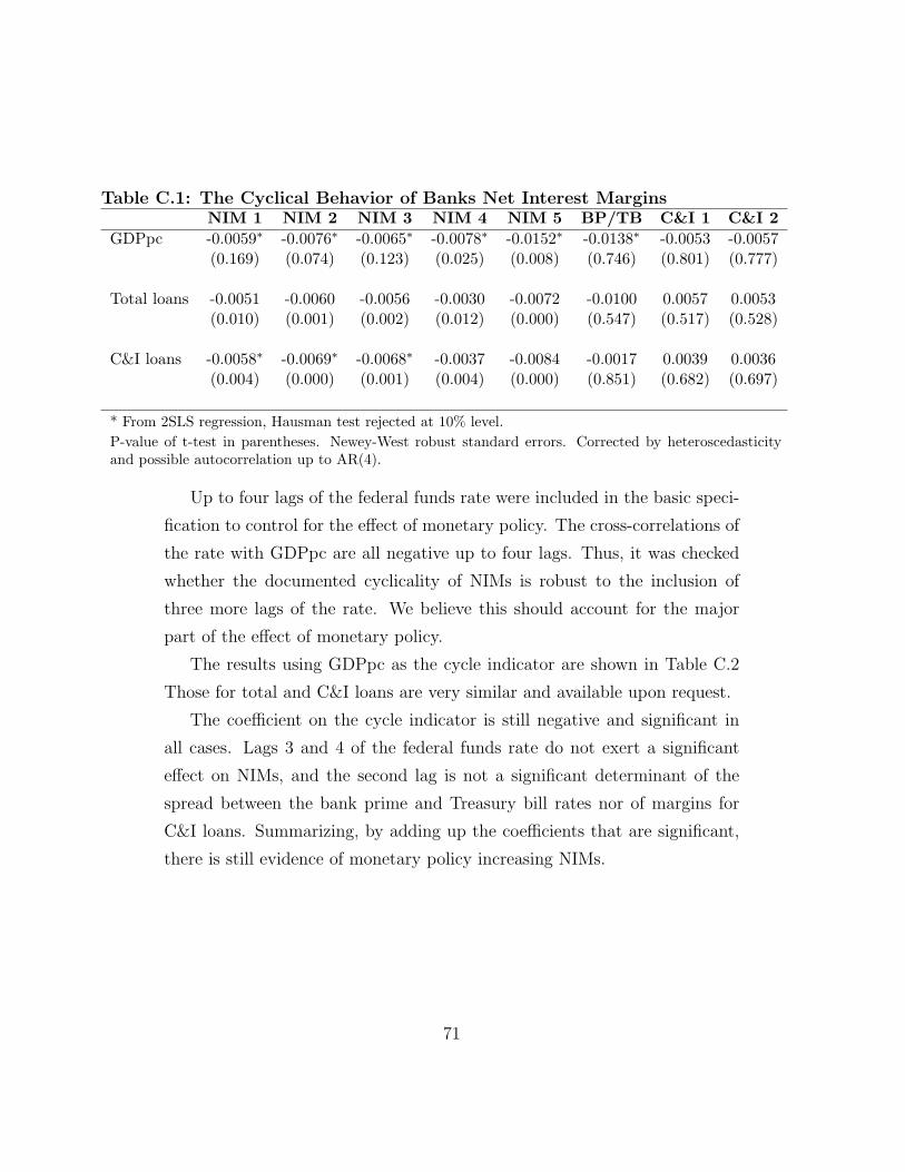
Table C.1: The Cyclical Behavior of Banks Net Interest MarginsNIM 1 NIM 2 NIM 3 NIM 4 NIM 5 BP/TB C&I 1 C&I 2
GDPpc -0.0059∗ -0.0076∗ -0.0065∗ -0.0078∗ -0.0152∗ -0.0138∗ -0.0053 -0.0057(0.169) (0.074) (0.123) (0.025) (0.008) (0.746) (0.801) (0.777)
Total loans -0.0051 -0.0060 -0.0056 -0.0030 -0.0072 -0.0100 0.0057 0.0053(0.010) (0.001) (0.002) (0.012) (0.000) (0.547) (0.517) (0.528)
C&I loans -0.0058∗ -0.0069∗ -0.0068∗ -0.0037 -0.0084 -0.0017 0.0039 0.0036(0.004) (0.000) (0.001) (0.004) (0.000) (0.851) (0.682) (0.697)
* From 2SLS regression, Hausman test rejected at 10% level.P-value of t-test in parentheses. Newey-West robust standard errors. Corrected by heteroscedasticityand possible autocorrelation up to AR(4).
Up to four lags of the federal funds rate were included in the basic speci-
fication to control for the effect of monetary policy. The cross-correlations of
the rate with GDPpc are all negative up to four lags. Thus, it was checked
whether the documented cyclicality of NIMs is robust to the inclusion of
three more lags of the rate. We believe this should account for the major
part of the effect of monetary policy.
The results using GDPpc as the cycle indicator are shown in Table C.2
Those for total and C&I loans are very similar and available upon request.
The coefficient on the cycle indicator is still negative and significant in
all cases. Lags 3 and 4 of the federal funds rate do not exert a significant
effect on NIMs, and the second lag is not a significant determinant of the
spread between the bank prime and Treasury bill rates nor of margins for
C&I loans. Summarizing, by adding up the coefficients that are significant,
there is still evidence of monetary policy increasing NIMs.
71
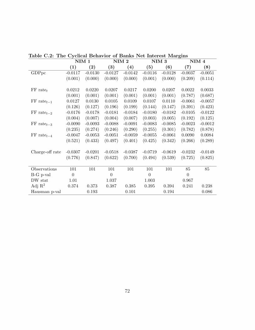
Table C.2: The Cyclical Behavior of Banks Net Interest MarginsNIM 1 NIM 2 NIM 3 NIM 4
(1) (2) (3) (4) (5) (6) (7) (8)GDPpc -0.0117 -0.0130 -0.0127 -0.0142 -0.0116 -0.0128 -0.0037 -0.0051
(0.001) (0.000) (0.000) (0.000) (0.001) (0.000) (0.209) (0.114)
FF ratet 0.0212 0.0220 0.0207 0.0217 0.0200 0.0207 0.0022 0.0033(0.001) (0.001) (0.001) (0.001) (0.001) (0.001) (0.787) (0.687)
FF ratet−1 0.0127 0.0130 0.0105 0.0109 0.0107 0.0110 -0.0061 -0.0057(0.126) (0.127) (0.196) (0.199) (0.144) (0.147) (0.391) (0.423)
FF ratet−2 -0.0176 -0.0178 -0.0181 -0.0184 -0.0180 -0.0182 -0.0105 -0.0122(0.004) (0.007) (0.004) (0.007) (0.003) (0.005) (0.192) (0.125)
FF ratet−3 -0.0090 -0.0093 -0.0088 -0.0091 -0.0083 -0.0085 -0.0023 -0.0012(0.235) (0.274) (0.246) (0.290) (0.255) (0.301) (0.782) (0.878)
FF ratet−4 -0.0047 -0.0053 -0.0051 -0.0059 -0.0055 -0.0061 0.0090 0.0084(0.521) (0.433) (0.497) (0.401) (0.425) (0.342) (0.266) (0.289)
Charge-off rate -0.0307 -0.0201 -0.0518 -0.0387 -0.0719 -0.0619 -0.0232 -0.0149(0.776) (0.847) (0.622) (0.700) (0.494) (0.539) (0.725) (0.825)
Observations 101 101 101 101 101 101 85 85B-G p-val 0 0 0 0DW stat 1.01 1.037 1.003 0.967Adj R2 0.374 0.373 0.387 0.385 0.395 0.394 0.241 0.238Hausman p-val 0.193 0.101 0.194 0.086
72
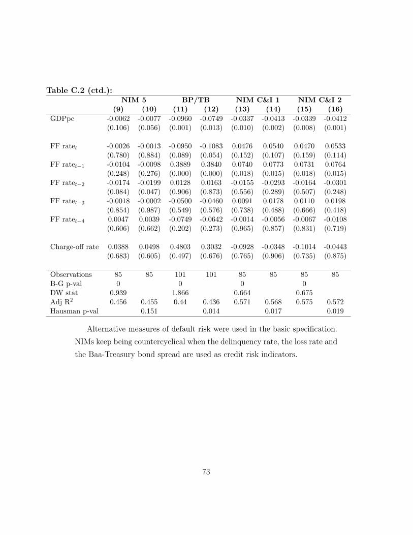
Table C.2 (ctd.):NIM 5 BP/TB NIM C&I 1 NIM C&I 2
(9) (10) (11) (12) (13) (14) (15) (16)GDPpc -0.0062 -0.0077 -0.0960 -0.0749 -0.0337 -0.0413 -0.0339 -0.0412
(0.106) (0.056) (0.001) (0.013) (0.010) (0.002) (0.008) (0.001)
FF ratet -0.0026 -0.0013 -0.0950 -0.1083 0.0476 0.0540 0.0470 0.0533(0.780) (0.884) (0.089) (0.054) (0.152) (0.107) (0.159) (0.114)
FF ratet−1 -0.0104 -0.0098 0.3889 0.3840 0.0740 0.0773 0.0731 0.0764(0.248) (0.276) (0.000) (0.000) (0.018) (0.015) (0.018) (0.015)
FF ratet−2 -0.0174 -0.0199 0.0128 0.0163 -0.0155 -0.0293 -0.0164 -0.0301(0.084) (0.047) (0.906) (0.873) (0.556) (0.289) (0.507) (0.248)
FF ratet−3 -0.0018 -0.0002 -0.0500 -0.0460 0.0091 0.0178 0.0110 0.0198(0.854) (0.987) (0.549) (0.576) (0.738) (0.488) (0.666) (0.418)
FF ratet−4 0.0047 0.0039 -0.0749 -0.0642 -0.0014 -0.0056 -0.0067 -0.0108(0.606) (0.662) (0.202) (0.273) (0.965) (0.857) (0.831) (0.719)
Charge-off rate 0.0388 0.0498 0.4803 0.3032 -0.0928 -0.0348 -0.1014 -0.0443(0.683) (0.605) (0.497) (0.676) (0.765) (0.906) (0.735) (0.875)
Observations 85 85 101 101 85 85 85 85B-G p-val 0 0 0 0DW stat 0.939 1.866 0.664 0.675Adj R2 0.456 0.455 0.44 0.436 0.571 0.568 0.575 0.572Hausman p-val 0.151 0.014 0.017 0.019
Alternative measures of default risk were used in the basic specification.
NIMs keep being countercyclical when the delinquency rate, the loss rate and
the Baa-Treasury bond spread are used as credit risk indicators.
73

Appendix D: Directions for Further Research- Robustness Checks
• Get comments from MU, John Seater and Hall (before we leave Durham),
maybe Loreta Mester once I am in Drexel.
• Try with 4 lags of the federal funds rate, because the cross-correlations
are all negative and significant. We did not try with more lags, but we
think that the biggest part of the effect of monetary policy should be
captured by 4 lags.
• Use the delinquency rate and the loss rate as alternative measures of
default risk. Find a credit risk measure that is significantly counter-
cyclical. The charge-off rate is countercyclical but not significantly.
• Try regression without any control except for seasonality and regulation
dummies.
• Try getting rid of the two interactions.
• HHI instead of share big as a measure of concentration. Or even add
HHI as a measure of concentration and leave the share of big banks as
a measure of compositional effects.
• Alternative measures for the costs of banks (alternative to deposits).
• Introduce a measure of the interest rate elasticity of the demand for
credit as an additional control.
• Try with alternative subsets of the set of controls. Given what we
discussed with Roger, it seems that this does not make much sense to
us, given our goal. Our econometric model is this one and any change
would imply an omission bias.
74
• PANEL DATA: It seems that we cannot justify the use of panel data
here. We should think about the 2nd derivative of the NIM with re-
spect to the business cycle indicator and one more bank-level measure.
Therefore, we would be interested in the first derivative with respect
to the cycle indicator (a time-series dimension) and then the derivative
of that with respect to a cross-sectional dimension variable. But we
are not interested in how bank-level variables can explain this macro
fact. Also, strategically, to differentiate ourselves (macro) from the IO
empirical banking literature.
Other papers use panel data because they focus on the empirical de-
terminants of NIMs in general and bank-level variables are important
determinants in that case. Not in our case where we want to explain a
macro fact, the cyclicality of NIMs.
75