[1]

On Understanding the Cyclical Behavior

of the Price Level and Inflation

William A. Brock

and

Joseph H. Haslag1

July 2, 2014

Abstract: In this paper, we examine the relationship between the price level and output and the inflation

rate and output at business-cycle frequencies. In the first part of the paper, we develop a methodological

approach based on the time series bootstrap adjusted for model uncertainty to characterize joint business

cycle correlations. In particular, we are interested in providing a characterization of the frequency that a

pair of correlation coefficients will occur. We apply this methodology to the contemporaneous correlation

between the price level and output and between the inflation rate and output. We apply linear filters to the

cyclical components, create a time series and compute the correlations. It is straightforward to construct

histograms of the two correlation coefficients. In the second part, we specify a model economy with a

form of rational inattention. In this setting, we perform numerical simulations to determine if the model

economy can generate correlations quantitatively similar to those observed in the data. It can.

JEL codes: C82, E31, E32

Keywords: model uncertainty, filter, price level, output

I. Introduction

For business cycle researchers, two facts have emerged in the post-World War II data. Because the

inflation rate is the direction of change in the price level over time, it is natural to expect that co-

movements between the price level and output are qualitatively the same as co-movements between the

inflation rate and output. However, there is evidence that the contemporaneous correlation coefficient for

the price level and output is negative and the contemporaneous correlation between the inflation rate and

output is positive. In other words, the price level is countercyclical and the inflation rate is procyclical.

Kydland and Prescott (1990) initiated this research line when they reported that after filtering for the

business-cycle component, the price level is negatively correlated with output.2 Other researchers began

testing the robustness of this finding. Cooley and Ohanian (1991) and Smith (1992) extend the sample.

1 The authors would like to thank Eric Young, Chris Otrok, Tim Cogley, Ana Maria Herrera, participants at the

Midwest Macro Meetings and University of Missouri Brown Bag seminar for helpful comments on an earlier draft of this paper. 2 Kydland and Prescott reported this result because it contradicted the maintained hypothesis that the price level

was procyclical. In their view, theory was needed to account for the negative relationship.

[2]

The two papers broadly agree that before World War II, the evidence suggests the price level was

procyclical.3 After World War II, however, the evidence is consistent with Kydland and Prescott’s finding

that the price level has been countercyclical.

Wolf (1991) asks whether the price level is countercyclical over the post-war sample period. He

distinguishes between business cycles before and after the 1973 recession. Wolf’s view builds on the

question, Are all business cycles alike?4 In particular, Wolf presents evidence from price indexes

constructed from consumer expenditure categories. Based on the temporal break and from the correlation

between movements in output and the price indexes, he concludes that the price level has been

countercyclical since the 1973 recession, but not before.

Cooley and Ohanian also consider the set of business cycle facts to examine the relationship between

the cyclical component of the inflation rate and output. They report that inflation rate is procyclical during

the post-war sample. Webb (2003) and Kanstantakapoulou , Efthymois and Kollintzas (2009) are more

recent contributions. Webb is especially clear on the stakes involved in the issue of procyclicality of the

price level. He states, “The issue is of particular importance to macroeconomists who must choose which

model to work with.”5 Kanstantakapoulou et al. investigate the robustness of countercyclicality of the

price level and procyclicality of the inflation rate for 9 OECD countries using quarterly data, 1960-2004.

For example, they state, “We examine the stylized facts …prices are countercyclical; inflation is

procylical.”6 Given the deterministic relationship between the price level and the inflation rate, the

qualitative difference deserves attention.

Researchers have debated the implications associated with a countercyclical price level. One debate

has centered on the competing role of demand shocks and supply shocks as a source or business cycle

fluctuations. Kydland and Prescott asserted the following: “We caution that any theory in which

procyclical prices figure crucially in accounting for postwar business cycle fluctuations is doomed to

failure.” (p.17, 1990).

Researchers responded along two fronts. One approach focused on the relationship between prices

and output at business cycle frequencies. In particular, den Haan (2000) asked why the unconditional

correlation coefficient the appropriate measure of comovement between the price level and output? In

doing so, den Haan proposes using correlations of k-step-ahead forecast errors from VARs which allows

the researcher a richer dynamic set of correlations. Based on this evidence, den Haan counters with the

3 In Cooley and Ohanian, the evidence is ambiguous before World War I. During the interwar period, they report

that the price level is procyclical. In Smith, the evidence is that the price level is procyclical before the Great Depression. 4 See Blanchard and Watson (1986) for a detailed discussion on this question.

5 See Webb (2003, page 69).

6 See Kanstantakapoulou et al. (2009, page 1).

[3]

argument that “a theory in which prices do not have some procyclical feature is, at best, missing a part of

the explanation of U.S. business cycle fluctuations.” (p. 5, 2000).

The other approach focused on showing that sticky-price models can account for relationship between

the price level and output. Chadha and Prasad (1994), Ball and Mankiw (1995) and Judd and Trehan

(1995) specify versions of sticky price models in which only demand shocks are considered. Each shows

that model economies are capable of accounting for the negative unconditional correlation coefficient

observed between some detrended versions of output and the price level.7 Rotemberg (1996) examines

forecastable movements in output and the price level, showing that they are negatively correlated. In a

sticky-price model with only demand shocks, Rotemberg can account for the relationship between the

forecastable parts of output and the price level.

Webb (2003) stresses the difference in behavior between commodity prices, final goods prices, and

wages over the business cycle. Webb argues that there are key differences in the price-setting institutions:

commodity prices are set in spot markets, final goods are set by slower-moving methods, and wages in

which the prices of different types of labor tend to move even slower than commodity prices over the

business cycle. Webb points out that the monetary regime plays a significant role; during the gold

standard, a procyclical price level is likely to become countercyclical in a fiat money regime. Webb cites

Wesley Clair Mitchell as providing the original logic for procyclical price level during the gold standard

period. Webb further argues that the procyclical property holds when “price level” is replaced by “rate of

change of the price level”.

While it is true that the relationship between the price level and output has been extensively studied,

but there is a hole in the literature regarding two unconditional correlations. Namely, to our knowledge no

one has tried to develop a model economy that can account for both the countercyclical price level and the

procyclical inflation rate. Haslag and Hsu (2012) examine the degree to which a phase shift can account

two facts. Specifically, Haslag and Hsu document the size of the phase shift that could account for the

pair of reported correlation coefficients. The approach does not explain why there is a phase shift.

Thus, there are two broad questions that come to mind in light of the literature. First, we focus on two

business cycle facts. One goal, therefore, is to develop a methodology that characterizes the joint

distribution function; our aim is to present a methodology that allows one to accurately characterize and

measure the level of uncertainty when there are joint patterns. Such a methodology permits one to

represent the probability of any particular data pattern in an empirically disciplined way that also respects

“model uncertainty.” We apply this methodology to the particular question of the correlation between the

7 The intuition rests on output being mean reverting. Given a positive aggregate demand shock, output increases.

Because prices were sticky, output would begin falling (mean reverting) and prices would increase eventually, causing real balances to decline and output to decline further. Of course, introduction of sticky prices into the model economy raises another question; specifically, why are prices sticky?

[4]

price level and output and the correlation between the inflation rate and output. In our view, the

methodology could easily be extended to characterizing the likelihood of multiple business-cycle

correlations. Second, we are interested in providing some theoretical model to account for these two facts.

To our knowledge, there is not a paper that has been able to account for the phase shift that is embodied in

the two unconditional correlations. There are various “sticky price” models, e.g. Rotemberg (1996), in

which the model economy can account for a positive correlation between output growth and the inflation

rate, but ignores≈ the relationship between output growth and the change in the inflation rate. We

investigate a form of “rational inattention” as a type of friction that could account for this pair of facts.

We then provide quantitative results from a model economy to support this view. We view this exercise

as an attempt to “measure” the strength of potential heterogeneity in expectations where some of the

expectational types are “backwards-looking” as a potential force in accounting for these two facts. More

generally, we investigate how far plausible dynamics of expectations themselves can go in explaining the

two facts. On this front, we show that one can account for the phase shift by matching the two

correlations. As such, our results constitute a contribution to the business cycle literature in the sense that

the introduction of rational inattention and robust control methods can account for the pair of correlations.

In addition, we examine the pair of correlation coefficients from two different filtering approaches.

Researchers have applied both trend-stationary and difference-stationary methods to identify the cyclical

component of economic time series.8 We consider both approaches. In both methods, the cyclical

component of the price level is negatively correlated with the cyclical component of output. In the trend-

stationary approach, which used the H-P filter, the cyclical component of the inflation rate is positively

correlated with the cyclical component of output. However, in the difference-stationary case, the cyclical

component of the inflation rate is not systematically related to the cyclical component of output. This is

consistent with Webb (2003, page 75) where he points out that the absolute value of the correlation is

much smaller using log-differenced data than linear detrended data.

1.1. On Model Uncertainty

The methodological contribution is related to the stance that was presented in Brock, Durlauf and

West (hereafter (BDW)) (2003) and (2007). In BDW, the stance was built on the notion of Bayesian

Model Uncertainty where prior probabilities were assigned to each model specification. After estimating

each model, the posterior probabilities were assigned based on relative likelihoods. Here, we simply filter

out the low-frequency components by applying two different methods of making the time series

(covariance) stationary; that is, trend stationary and difference stationary in the sense of Nelson and

Plosser (1982). We then estimate models with the resulting filtered data and report how the probability of

8 Nelson and Plosser (1982) identified this source of model uncertainty in their study of macroeconomic time

series.

[5]

the pattern of interest depends upon the method of detrending. We can compute the probability that the

pattern of interest in a data disciplined way by using the estimated standard errors (under appropriate

distributional assumptions, e.g. Gaussian) of the parameters of each model fitted to the filtered data. Of

course, one could do this same exercise taking into account the uncertainties in the estimated parameters

of the trend model also. We ignore this extra source of uncertainty in this paper in the interest of

simplicity. We report histograms that show the part of the space where the pattern of interest holds with a

set of “skyscrapers” whose height gives the probability of that grid of the space. For example, we are

basically just using bootstrapping (Efron (1982), Efron and Tibshirani (1986)) to estimate the probability

of the pattern of interest, i.e. the probability that the “stylized fact” under scrutiny in this paper holds

under each method of detrending. All this will be explained in greater detail below.

One of the main points we want to get across in this paper is that we think this methodology is a

useful way to present data patterns of interest in macroeconomics together with a measure of the

uncertainties surrounding each such pattern. To put it another way, we are arguing that such a

methodology can be helpful when presenting joint “stylized facts” in macroeconomics.

In this particular application, we apply a single-equation, univariate autoregressive filter to create

time series of the price level and output. We then compute the contemporaneous cross-correlations for the

price level and output and the inflation rate and output. With the correlation coefficients, we can compute

the likelihood that the filter yields countercyclical price level and procyclical inflation. By adopting the

autoregressive filter, the approach stresses the role of persistence and goodness-of-fit to infer the

likelihood. In other words, there are three key factors that play roles in determining the likelihood of the

observed cross-correlations; namely, (i) the estimated values of the relative persistence in the cyclical

components, the standard errors of the parameter estimates and (ii) the unexplained variation in the

cyclical components. The single-equation methodology allows us to assess the importance of each factor.

In addition, we apply a VAR approach to simulate the time series for each variable. In this setting, we

observe a better fit in the sense that the distribution is massed over the joint event that the price level is

countercyclical and the inflation is procyclical. In contrast, the maximum probability of this joint event

range is 62 percent in the single-equation method. When we use the first-difference approach to filtering

out the cyclical component, the inflation rate is acyclical. We take the opportunity to demonstrate that the

methodology is flexible; indeed, we find that the joint likelihood is 82 percent that the price level

correlation lies within the range of 0.0 to -0.2 together the inflation rate correlation lies in the range of -

0.1 to 0.1. In general, one can compute the frequency for any joint values of the two correlations. In our

view, it can be very useful for researchers to compute the likelihood of joint empirical regularities as a

way to gauge the joint strength of a wide range of empirical regularities.

[6]

1.2 On rational expectations and rational inattention

“Rational inattention” is one of those labels that has been used to describe more than one approach

used in the literature, e.g. Sims (2003) and Reis (2006) are two prominent examples. Hence it is

important for us to be precise and describe exactly how we are using the label, “rational inattention.” We

are using “rational inattention” in the sense that there are “backwards-looking” expectations as in Branch

and Evans (2011), De Grauwe (2011), and Massaro (2013), as well as “forward-looking”, i.e. rational

expectations, also see Brock and Hommes (1997). Brock and Hommes present a framework which is

much simpler than the more realistic frameworks of the above authors, where it is costly to acquire the

information necessary to form rational expectations, whereas backwards-looking expectations are free.

Here, we use an off-the-shelf money-in-the-utility function model, adding a form of rational inattention to

determine whether this type of information friction can account for the phase shift in filtered price level.

We study a special case of these costs in which agents purchase inexpensive “backward-looking” price

expectations. Our quantitative analysis is encouraging in the sense that there is a reasonable set of

parameters that result in countercyclical prices and acyclical inflation. The numerical results are

consistent with the presence of a phase shift and qualitatively match the results obtained when we assume

the cyclical components are derived from a difference-stationary process.

To further illustrate we present the solution to the forward-looking rational expectations equilibrium.

In this way, we can contrast the notion of price stickiness that is imparted by our particular form of

rational inattention. In other words, the comparison helps one see why rational inattention works the way

it does. Our results tend to confirm the role that forward-looking rational expectations plays; namely, that

prices adjust so quickly to new shocks that the direction of the change in the price level dominates the

direction of change in the inflation rate. We explore the possibility that interaction with persistence of

other forces, e.g. taste shocks and the desire of our representative agent for robustness against possible

mis-specification of its economic environment may blunt the usual effect of rapid adjustment of the price

level under rational expectations. We believe the modest extension of the framework we use—i.e., that of

Woodford (2003)—may be of independent interest. Returning to the standard effect of rational

expectations, to put it in other words, we wish to stress that, forward-looking rational expectations

imparts phase-synchronicity between movements in output and movements in the price level. Such

synchronous movements explain why models economies incorporating rational expectations cannot

account for the price level being countercyclical and the inflation rate being either procyclical or

acyclical. After having made this well-known point to set the stage, we show how minimalist backing

off from rational expectations in the sense of maintaining rational expectations on long term trends but

allowing departures from rational expectations on shorter term fluctuations about trend can explain the

[7]

two facts as well as generate plausible dynamics of shorter term fluctuations about trend. Furthermore

our treatment of shorter term dynamics of expectations via perturbation techniques around dynamic

intertemporal equilibria of the model and our introduction of robustness concerns on the part of the

representative agent in the model may be of independent interest.

The paper outline is as follows. In Section 2, we consider an example that analytically illustrates the

methodological approach. We construct the numerical analyses in Section 3 for both the H-P filter and

first-difference measures of the cyclical components. Section 4 develops the model economy and reports

the numerical results. In particular, we use the model economy to provide some analytical support and

understanding of forces that produce negative correlation of the cyclic component of the price level

(positive correlation of inflation) with the cyclic component of output by using the model of Woodford

(2003, Chapter 2). Here is where we show that minimalist departures from rational expectations where

rational expectations are maintained on trends but relaxed for shorter term fluctuations in expectations

(which we justify by reference to recent work on the dynamics of inflation expectations at the Cleveland

Fed and elsewhere) easily generates plausible shorter term dynamics that are consistent with the two

correlations. We also show how to extend this standard model to robustness in the spirit of Hansen and

Sargent (2008) and the recent work of Anderson, Brock, Hansen and Sanstad (2014) in Section 5.

Finally, Section 6 is a brief summary, conclusions, and suggestions for future research.

II. Model Uncertainty by Linear Approximations: An Analytic Example

In this section, we consider a specific autoregressive process to illustrate how the various components

affect the likelihood that the correlations will exhibit the pattern in the data.

Suppose both the price level (p) and output (y) (in log levels) are capable of being decomposed into

trend components and cyclical components. Formally,

, where . The superscript T

denotes the trend component while the superscript C stands for the cyclical component. We start by

estimating low order AR (q) models to the cyclical components. We find that an AR(1) and an AR(2) fit

well as specified in (1) and (2) below. The low orders of these processes allow us to prove the two

Lemmas and Proposition 1 below. These simple results are useful to uncover sufficient conditions on the

Data Generating Processes (DGP) for the cyclical components for the cyclical component of the price

level to be countercyclical and the cyclical component of inflation to be procyclical.

Henceforth, for this initial part of the paper, we assume that the cyclical component of the price level

follows an AR(1) process while the cyclical component of output follows an AR(2) process. Thus,

(1)

(2)

[8]

The cyclical components are computed as deviations from trend. Assume that the cyclical

components for both the price level and output are mean zero, stationary processes. We drop the

superscripts to write the implication of the stationary process as [ ] [ ] [ ], where

[ ] denotes the covariance of the cyclical components of the price level and output. Under these

assumptions, the sign of the covariance determines the sign of the contemporaneous cross-correlation.

We derive the expected value of the product of the cyclical component of the price level and output

by substituting equations (1) and (2) into the covariance expression, yielding

[ ] ( ) [ ] [ ] [ ]

After rearranging and simplifying, we obtain

[ ] [ ]

[ ] (3)

Based on equation (3), we derive the following lemma.

Lemma 1: With [ ] ( ) and with [ ] ( ) , then the sign of [ ] is

negative.

Equation (3) tells us that the sign of the cross-correlation coefficient depends on the sign of the

covariance of the unexplained errors from the two AR processes that characterize the cyclical components

of the price level and output, respectively. If the residuals are independent, then the correlation coefficient

is zero. However, if the unexplained errors are negatively correlated and the denominator is positive, for

example, then the correlation coefficient is negative. Note further that the denominator depends on the

persistence of the two cyclical components. With [ ] for example, greater persistence in price

level or in output makes it less likely that the correlation between the price level and output will be

negative.

Next, we turn to the covariance between inflation and output. Let [ ] [( ) ] denote

the covariance between the inflation rate and output. Substitute for the date-t price level from equation (1)

and for output from equation (2), yielding

[ ] [ ] {

} (4)

where . From which, we derive the following Lemma.

Lemma 2: With [ ] ( ) , the sign of [ ] if and only if

[ ] ( ) .

Equation (4) indicates that the sign of the correlation between inflation and output again depends on

the correlation between residuals. If the residuals are negatively correlated, for example, the bracketed

term must be negative for the cyclical components of the inflation rate and output to be positive.

Note that the condition in Lemma 2 involves the denominator in Lemma 1. Therefore, the

combination of conditions in Lemmas 1 and 2 create a partition for the space of estimated coefficients

[9]

that must be satisfied for the price level to be countercyclical and the inflation rate to be procyclical. We

derive those conditions in the following proposition.

Proposition 1: Based on the conditions derived in Lemmas 1 and 2, the price level is

countercyclical and the inflation rate is procyclical for

if [ ] and

[

] if [ ] .

By writing down the conditions in Lemma 1 and Lemma 2 and solving for the inverse of the

persistence coefficient in price level equation, we obtain the conditions in Proposition 1. Note that the

denominator that yields [ ] < 0 depends on the sign of the covariance between the unexplained terms.

For example, if [ ] , then [ ] if the denominator is positive. It follows from Lemma 2 that

[ ] if the numerator is negative.

Combining the conditions in Lemmas 1 and 2, the two correlation coefficients are opposite signs if

if [ ] In contrast, if [ ] , the condition is [

].

The upshot of Proposition 1 is that there exists a range of parameter values that are consistent with the

joint observation that the price level is countercyclical and the inflation rate is procyclical. In other words,

Proposition 1 derives the values for one specific illustration of a linear autoregressive process that will

yield the joint business cycle fact. If the residuals from the two autoregressive processes are negatively

correlated, for example, Proposition 1 indicates that the price level cannot be “too persistent” relative to

the persistence in the output equation for the joint business-cycle observation to hold. Conversely, if the

residuals are positively correlated, the price level must be persistent enough relative to the persistence

observed in the output equation for the price level to be procyclical and the inflation rate to be

countercyclical.

To be more concrete, consider a case in which the cyclical component of the price level is a random

walk. If the residuals are negatively correlated, for example, Proposition 1 tells us that the condition

which jointly satisfies countercyclical price level and procyclical inflation rate cannot be satisfied. The

first inequality in the sequence fails to be greater than one. For the case in which the residuals are

positively correlated, then with positive coefficients in the AR process for output, the condition can be

satisfied.

Consider a case in which both the output and the price level follow AR(1) processes. With

, we present the conditions for the pair of correlations in the following proposition:

Proposition 2: If [ ] , then the price level is countercyclical and the inflation rate is

procyclical, in expected value, if . (See Appendix)

[10]

Proposition 2 reduces the expected sign of the correlation coefficients to persistence in the

cyclical components. The key is that the cyclical component of output lies outside the unit root and the

product of the two persistence coefficients is less than one. It follows that the persistence in the cyclical

component of the price level is “low enough” to satisfy the condition.

While we will see below that the AR(q) processes for detrended price level and detrended real output

that we identified by standard time series methods are higher order than 1 and 2, we believe our Lemmas

and Propositions help understand what kinds of persistence properties are needed into order to be

consistent with procyclical inflation rate and countercyclical price level.

III. Model Uncertainty and Histograms

The data are quarterly observations from the United States for the period 1947:1 through 2007:4.

Output is measured by real GDP and the chain-weight index for personal consumption expenditures. We

use the H-P filter with to obtain the filtered, or cyclical, values of output and the price level.

In addition, we consider cases in which the cyclical component is constructed by first differencing the

data. Formally, and

.9 For completeness, note that the DS-cyclic

component of the inflation rate is defined as follows:

.

We begin by estimating the correlation coefficients for the different measures of the cyclical

components. Table 1 reports the summary statistics for the HP filtered and the DS-cyclic measures. We

are particularly interested in the contemporaneous correlations. In the HP filtered series, the cross

correlations are different. The Bartlett standard error of this estimate is

√ for our sample.

Consequently, the evidence indicates that the price level is countercyclical and the inflation rate is

procyclical. With the DS components, however, the contemporaneous correlation coefficient for the price

level and output is -0.145 and the contemporaneous correlation coefficient for the inflation rate and output

is -0.013. Thus, an important difference emerges based on the approach used to construct the cyclical

components; we can reject the null hypothesis that the price level is zero and hence it is countercyclical,

but with the DS measures, the inflation rate is acylical.

Overall, the summary statistics paint a different picture based on how the cyclical components are

measured. Even with the quantitative difference present in the two detrending methods, there is a

common thread that emerges regardless of how the cyclical components of the price level and output are

measured. Both the HP filter and the first-difference approach are consistent with the notion that there is

9 In the first-differencing case, the cyclical components have other natural interpretations. By first-differencing the

log of output and the log of the price level, the correlation, ˆ py , is between output growth and inflation.

Further, ˆ y is between output growth and the change in the inflation rate.

[11]

evidence of phase shift between the cyclical component of the price level and the cyclical component of

output. The phase is not as pronounced when we use the DS approach, but the phase shift can account for

the different signs in the unconditional correlation coefficients.

3.1 Single Equation Approach

We begin by applying single, linear regressions to fit the time series. We use AIC to select the lag

length in the estimation part. For the price level, the AIC selects four lagged values of the price level for

both the HP and the first-difference measurements of the cyclical components. For output, AIC chooses

three lagged values whenC

tx is measured by the HP filter and five lagged values when measured by first

differences. The coefficients and standard errors are reported in Table 2.

Armed with these equations and the residuals, our aim is to employ standard bootstrapping methods

to generate simulated time series. The simulated series can then be used to estimate correlation

coefficients and we can assess the likelihood that a particular observed pattern of the correlation

coefficients is present. In more detail we wish to estimate the probability that

cov( , ) 0,cov( , ) 0C C C Cp y p y where the two covariances are estimators under the DGP’s (1) and

(2). Since the two covariances must be estimated on our sample of length T, therefore we use the time

series bootstrap, e.g., as described in Berkowitz and Kilian’s survey (2000). Specifically, we use a time

series bootstrapping procedure to compute the likelihood that the joint correlation coefficient is

represented by

ˆ ˆ ˆP{ 0, 0}C C C Cp y p y

(5)

where

1

1 2

ˆ ˆ(1/ ) , ( ) (1/ ) ( )T T

C C C C C C C C C

t t t t t

t t

p y T p y p y T p p y

(6)

1

1 1 2

ˆ ˆ ˆP{ 0, ( ) 0}

(1/ ) {1[(1/ ) 0, (1/ ) ( ) 0]}

C C C C

B T Tb b b b b

t t t t t

b t t

p y p y

B T p y T p p y

(7)

1

1 1 2

ˆ ˆ ˆP{( , ( ) ) } (1/ ) {1[((1/ ) , (1/ ) ( ) ) ]}B T T

C C C C b b b b b

t t t t t

b t t

p y p y A B T p y T p p y A

(8)

[12]

Where the superscript “b” indicates the bootstrapped sample generated by the estimated equations. The

implementation of Equations (7) and (8) is described in detail below. We estimate the single equation

using our sample of length T for a given method of detrending. We compute the sample variances and

covariances of the estimated residuals to get an estimate of the variance matrix. We then used our

estimate of the variance matrix of the residuals to compute standardized residuals. Call these

standardized residuals, ˆ ˆ{ , , 1,2,..., }yt pt t T which have variance one and covariances zero by

construction.

Overall, we followed the procedure outlined in Berkowitz and Kilian (2000) for each of the pair

of AR(q)’s estimated for the detrended logs of the price level and real GDP per capita with a small

modification to estimate the covariance between the estimated residuals between the price level and real

GDP per capita for our standardization procedure. We start with the HP filtered measure of the detrended

log price level and log output. We continue to report results for both the measurements of C

tp and C

ty

developed from the HP filter and first-difference methods.10

In this way we did B = 10,000 replications

of this bootstrap procedure to compute (7) and (8). Doing this procedure we obtained

ˆ ˆ ˆP{ 0, ( ) 0 | } 0.227C C C Cp y p y HP . Note that we added the “|HP” to indicate that we

held the detrending fixed throughout the B replications.

Figures 1 and 2 present the histograms for the bootstrap based on detrending using the HP filter

and the first-difference. In addition, we select the lag length for both cases using AIC. In the first-

difference case, ˆ ˆ ˆP{ 0, ( ) 0 | DS} 0.331C C C Cp y p y , where “|DS” designates the first-

difference method of detrending.11

Because the first-difference measure yields different patterns for the

10

The fitted regressions are: 2

2

2.43 0.011* 0.000005*

7.45 0.01* 0.000008*

C

t t

C

t t

p t t p

y t t y

The estimated coefficients are significant at 5 percent levels in every case. The results reported in this paper are qualitatively the same when we use the time-trend approach to measure the cyclical components of the price level and output.

11 Brock, Durlauf, and West (2003), (2007) recommended a form of model averaging in order to reflect

the “additional” uncertainty due to “model uncertainty”. E.g. in view of arguments in the literature for both TS and DS detrending methods and in view of the difficulty of short time series data sets typical in macroeconomics in distinguishing between TS and DS methods, we might attach equal credibility of ½ to each of these two methods.

In that case we might wish to bootstrap compute ˆ ˆ ˆP{ 0, ( ) 0 | }C C C CEp y E p y DS and, perhaps, not only

compare to evaluate the “sturdiness” of the joint fact to the method of detrending, but also report the average

ˆ ˆ ˆ ˆ ˆ ˆ(1/ 2)P{ 0, ( ) 0 | } (1/ 2)P{ 0, ( ) 0 | }C C C C C C C CEp y E p y TS Ep y E p y DS as a more

[13]

cross-correlation coefficients and because the methodology is flexible with respect to the questions we

can ask, we compute ˆ ˆ ˆP{ 0.25 0, 0.1 ( ) 0.1| DS} 0.462C C C Cp y p y . In other

words, the single-equation approach indicates that the likelihood is 46.2 percent that the price-output

correlation is between 0 and -0.25 and the inflation-output correlation coefficient is between -0.1 and 0.1.

Note that the histograms indicate that the events are massed around the combination that the two

simulated correlation coefficients are equal to zero. The reason is straightforward. In both single-equation

approaches, the residuals are uncorrelated. We observed in the simple AR processes used to derive the

analytical results in Proposition 1, the two correlation coefficients depend on the residuals. Indeed,

Equations (3) and (4) express the two correlation coefficients as linear functions of the correlation

between two residuals, and . Based on Equations (3) and (4), if the two residuals are independent,

both the price level and the inflation rate will be acyclical. Our numerical results are consistent with the

Proposition 1; by adding a random term to the parameter estimates, our bootstrapping results indicate that

the central tendency is consistent with the analytical results derived in Equations (3) and (4). In other

words, the two correlation coefficients tend to be massed around zero.

3.2 VAR approach

In addition to the single-equation approach, we estimate a bivariate VAR. The VAR is expressed

in terms of the cyclical components of the price level and output and the lag length is set at two. The

coefficient estimates and the standards errors are reported in Table 3 for the HP Filter approach and Table

4 for the first-difference approach.

We then simulate the time series using the coefficient estimates, the standard errors of the

coefficients and the standard errors of the each VAR equation. Based on the simulated time series,

repeated 10,000 times, we compute the correlation coefficients for the price level and output and for the

inflation rate and output. Since we simply estimated each row of the VAR as we did the AR(q)’s above,

and since we estimated the covariances of the residuals the same way we did above, we repeated the

bootstrapping procedure we did for the two AR(q)’s above, for our VAR. We present the histogram of

the correlation coefficients using the HP filtered measured of the cyclical components in Figure 3. As

Figure 3 shows, there is a dramatic change in the distribution of the correlation coefficients when

compared with the histograms generated by the single equation approach. Specifically, the distribution

appropriate statement of the joint fact. Or, better yet, the weights of ½ could be replaced with relative likelihoods as in Brock, Durlauf, and West (2003,2007).

[14]

presents events in the correlation coefficient between the price level and output is negative and the

correlation coefficient between the inflation rate and output is positive. Thus, there are 10,000 cases that

satisfy the joint condition in the VAR compared with cases reported in the single equation approach

ranging from 2300 to 3400 cases.

For the DS-cyclic components, we use the VAR to create 10,000 simulated time series. We then

compute the price level-output correlation and the inflation-output correlation for each of the 10,000

series and plot the resulting histogram in Figure 4. Based on this histogram, we find that for 52.6 percent

of the time, the price level-output correlation is negative and the inflation-output correlation is positive.

We also consider the case in which the price level-output correlation lies between 0 and -0.2 and the case

in which the inflation-output correlation lies between -0.1 and 0.1. In the first-difference VAR approach,

this occur 0.42 percent of the time. This is a sharp decline in the frequency of observations that fit into the

“bin” corresponding to the observed correlations in the actual data. In Figure 4, we see that the frequency

of correlations are massed at values of the price-output-correlation being greater than 0.3. It appears that

the chief reason behind the low-frequency performance lies with the fitness of the output equation. The

adjusted R-squared is 0.13 for the output equation. The R-squared values in the HP-Filter VARs is much

higher with values of 0.77 for the output equation and 0.89 for the price equation. Simply put, the

characterization of the frequency is a reflection of the goodness of fit.

Overall, we develop a methodology that allows us to construct simulated time series for the price

level and output. Once, we have the price level series, it is straightforward to construct the inflation rate

series. The key to the simulation process is to estimate linear models and then include uncertainty with

respect to the fit of the equation and to the coefficient estimates, as well as uncertainty about which model

to be fitted and which detrending method to be used. Once such model uncertainty is appropriately taken

into account, we can construct histograms for any joint business cycle facts. This numerical approach then

permits frequency questions regarding the joint statistics. In our view, the methodological development is

a useful tool for studying multiple moments in a variety of economic applications, especially in business

cycle contexts where people are interested in numerically assessing the likelihood of multiple stylized

facts

IV. Theory to account for the pair of cross-correlations

We consider a dynamic, stochastic general equilibrium model in which money enters directly into the

utility function. The MIUF approach does not take a stand on the friction that accounts for why fiat

money is valued in the economy. Our aim here is to take an off-the-shelf model economy, modify it in a

[15]

minimalist direction by inserting heterogeneous expectations, and derive the conditions in which we could

account for the pair of observations presented in this paper.

Here is our main motive for using such a well-known off the shelf model. We wish to show why a

purely rational expectations version cannot account for this particular joint fact. By using such a well-

known strawman, it is straightforward to modify it in one particular dimension to first see how far that

modification can go towards “explaining” the joint fact. By introducing backwards looking beliefs into

this standard model, we numerically show that we can generate a phase shift. Then, ultimately, we would

like to move in the direction of Branch and Evans (2011), De Grauwe (2011), and Massaro (2013) by

introducing an “ecology” of heterogeneous beliefs into this standard model where fully structural rational

expectations are part of the ecology but are only available at a cost and where the fractions of each type of

belief change over time depending upon relative performance histories. By “fully structural” here we

mean the rational expectations believers take into account the effect of the other believers upon an

equilibrium. Simpler versions of this kind of model are treated in the references above and other papers

they refer to. However, the infinite horizon together with the requirement that the rational expectations

beliefs are “fully structural” in the sense we defined above make the model intractable. Hence we chose

the simpler route of comparing two polar cases: (i) all believers are the same type of backwards

believers, (ii) all believers are fully structural rational expectations believers. We will see that the model

with beliefs of type (i) can account for the joint fact.

We think of this exercise is a useful complement to the received approaches, e.g. Rotemberg (1996),

Woodford (2003), and numerous others who have introduced “sticky prices” either by Calvo’s method

(see Chapter 4 in Aghion, Frydman, Stiglitz, and Woodford (2003) for an improved and updated version

of Calvo’s method) or by introducing “sticky prices” via adjustment costs as in Rotembeg (1996).

However, some of these methods of introducing “sticky prices” have been criticized by Robert Lucas in

Aghion et al. (2003, page 138). More precisely he said firms (or consumers) should not be “…locked

into a pricing policy that is completely unsuited to the new policy regime. They understand this new

regime fully, but they just cannot act on this knowledge…” We are thinking along similar lines as Lucas

where “pricing policy” is replaced by “belief dynamics” where the belief dynamics changes in response

to relative past performance as in Branch and Evans, De Grauwe, or Massaro.

There are infinite number of discrete time periods with t = 0,1,2,… There is a single, perishable

consumption good. The economy is populated by a measure-one continuum of representative agents. At

each , each agent is endowed with income represented by where P denotes the price level and

y is income measured in units of the consumption good.

[16]

Formally, let the representative agent solve the following infinite-horizon, discounted problem:

{∑ [ ( ) (

)]

}

(9)

where for j = c, m is a taste shock, following Woodford (2003, Chapter 2), for consumption

and real balances, respectively. Further, let increases (decreases) in the money supply over time be

distributed as a lump-sum payment (tax) represented by τ. Finally, M is the quantity of money balances

held by each person. The functions, U(.) and V(.), are twice continuously differentiable, strictly concave.

The marginal utility of each good is nonnegative. Woodford (2003, Chapter 2) considers both the

“cashless economy” case, V(.) = 0 and the “frictions” case where V(.) is non zero. He discusses the role

of the taste shocks as well as various money supply and interest rate rules of the Central Bank in this

framework for both cashless economies and monetary economies using this framework. We just take his

model “off the shelf” here and use it to study the set of real output, money supply, taste shocks and the set

of preferences that produce negative (positive) correlations between the cyclic components of the price

level (inflation) with the cyclic component of real output. Woodford’s model does not require that the

utility function be “separable” in consumption and real balances as we do in (9). We impose separability

for simplicity of the pricing formulas below. We leave it to future research to investigate non-separable

utility functions as well as recursive and risk sensitive preferences.

In this economy, agents are price takers. The sequence of shocks to tastes and income are drawn

from a distribution with positive supports. It is straightforward to derive the first-order necessary

conditions for utility maximization. Formally, the Euler equation is

( )

(

) [

( )( )] (10)

The money supply rule is:

, where ( ) where [ ].

In other words, the general setting is one in which the change in money supply depends on lagged output,

the lagged price level and the exogenous tastes shocks. The function is written broadly enough to

encompass money supply rules such as the Friedman k-percent rule or McCallum’s base rule as well as

more exotic versions. The numerical analysis will focus on a k-percent style rule, but these could be

easily modified to be cyclically dependent or an elastic supply rule.

[17]

The goods market clears when the quantity of goods consumed equals the quantity of goods

available. Thus, for equilibrium concepts that require market clearing, the goods market condition is

represented as .

To obtain some analytical results, we specify specific functional forms. For example, let ( )

( ) (

) (

). Further, let real income grow at rate so that after taking logs, we get

where { } is a stationary process and “tildes” are used to denote log transforms of

the variables. Let where is given and ( ) Thus, real income is

difference-stationary in this setup. We consider two polar cases of price expectations: (i) Backward

looking and (ii) Forward looking, i.e. rational expectations. The second case is structural rational

expectations. We treat the rational expectations, forward-looking case first.

4.1 Forward Looking Rational Expectations

The next step is to demonstrate what the correlations would look like in this model economy with

forward-looking expectations. By examining this case, we can learn why the expectation formation plays

a potentially important role in accounting for the phase shift present in the cyclical components of the

price level and output. It is well known that this type of model has difficulty in accounting for the

correlation patterns we are after in this article. This has been known for a long time and was a motive for

researchers to move towards “sticky price” models like Rotemberg (1996), Woodford (2003) and others

in the New Keynesian tradition. In the flexible-price versions, demand shocks could not account for

countercyclical prices. More generally, money, being an asset, has a “price” 1/t tP that “jumps” too

fast in response to new information, i.e. it is a “jump” variable. Hence researchers built models that

introduced different methods of “clamping down” on this jump variable by forcing it to move in a

“sticky” manner. But a criticism above and beyond criticisms like Robert Lucas’s in Aghion et al. (2003)

is that work on “design limits” like that of Brock, Durlauf, and Rondina (2013) suggests that there is a

“waterbed” type effect; that is, if the researcher squashes down variance in one variable in a dynamical

system, the variance is likely to “pop up” somewhere else. This notion can be made precise in the context

of linear control dynamics in the frequency domain. But one might worry if this kind of thing can happen

more generally. In order to show the jump variable phenomenon in, perhaps, a more transparent way than

received to date, we deliberately write the standard model in asset price equation form and study the result

below.

With forward- looking, rational expectations, the pricing equation becomes,

[18]

, 1 1 1( / )( / ) {( / )( / ) }t mt ct t t t c t ct t t taY M E Y Y (11)

Consider a case in which taste shocks are set equal to one for each date, 1 1,t tg m

t t t tY Y e M M e . We

treat { / }t taY M as a dividend process, solving (11) recursively forward as in asset pricing theory. We

obtain,

2

1 2{1/ [ / / ...]}t t t t t taY M E M M (12)

assuming the “no bubble” condition so that the tail term goes to zero. Note the conditional expectation,

tE in (12), limits the money supply processes that we can consider and still maintain easy analytical

tractability. If

1

1 , 1,2,...sm

s sM e M s

(13)

where the process, { }sm is IID with finite mean, m and finite variance, we may write the solution (12) in

the form,

( / ){1/ (1 )}m

t t taY M Ee (14)

Note that no restriction has been made on the real output process in getting this solution. Here, the

cyclical component is treated as difference-stationary log levels. Since this analysis applies to the

difference-stationary representation, we use the DS-cyclic component. As such, we may now use (14) to

compute the covariances of the DS-cyclic components of the price level and inflation with the DS-cyclic

component of real output. We have,

cov( , ) cov( , )C C

t t t t tp y m g g (15)

1 1 1cov( , ) cov( ( ), )C C C

t t t t t t t tp p y m g m g g (16)

These two equations are the basis for the analysis of the correlations in a rational-expectations model.12

We start with the simplest case as a means to shed light on two correlations. Specifically,

consider a case with a shock to output growth alone. We assume that the money supply is constant over

time and output growth follows an AR(1) process: 1 , 1,2,...t g g t gtg g n t where { }gtn is IID

12

The derivation of the equations below are in Brock and Haslag (2014).

[19]

with zero mean and finite variance. By Equation (15), we know the price level is countercyclical in this

model economy. Further,

1cov( , ) cov( , ) / (1 ) 0.C C C

t t t gt gt gp p y n n (17)

Equation (17) indicates that the inflation rate is countercyclical. With forward-looking agents, the price

level and output are in phase because consumers anticipate the persistence in output. Forward-looking

consumers, therefore, generate a cycle such that movements in the price level occur in phase with output.

With this setup in place, we can relax assumptions to see how they affect the two correlations.

For example, consider a case in which the money growth is stochastic. With ( , ) 1t gtm n , we obtain

1/2cov( , ) ( , )[var( ) var( )]t gt t gt t gtm n m n m n . (18)

If the variance of money growth is large enough relative to the variance of the DS-cyclic component of

real output, i.e., 2 2var( ) var( ) / (1 )t gt gm n , then the inflation could be countercyclical, but the

correlation with the price level will be “too large,” equaling minus one.

Following Woodford (2003, Chapter 2, pages 102 and 103), we consider the role of taste shocks

in the utility function in the MIUF model. If, for example, the Central Bank is trying to implement a

specific policy, e.g. inflation targeting or price level targeting, then the real disturbances modeled by taste

shocks could play an important role. We assume that the price level is countercyclical. Let

, 1

, 1 , , 1,2,...m t

m t m te t

where ,{ }m s is IID with finite mean, m , and variance. Following the

solution procedure used above, we obtain

1/ { / [ '( , ) ]}{1/ (1 )}m m

t t mt t ct tP a u Y M Ee

. (19)

Because Equation (19) permits just about any specification of the utility function ( , )t ctu Y as well as just

about any specification of the { },{ }ct tY processes, there are several new channels that could lead to

inflation being acyclical, given that the price level is countercyclical.

We consider with log utility represented as ( , ) ln( )t ct ct tu Y Y . The implication is that the

equilibrium price level is represented as

(1 ) /{ / }m m

t t ct mt tP Ee M a Y

(20)

[20]

From this, we obtain

, 1 ,

1

, 1 , 1 , 2 1 , , 1 1

cov( , ) cov(ln ln , )

cov( , )

cov(ln ln (ln ln ) ( ) ( ), )

C C

t t ct c t t m t t t

C C C

t t t

ct c t c t c t t t m t m t t t t

p y m g g

p p y

m m g g g

(21)

We may now use (21) to take logs and compute the covariance of the DS-cyclic component of the price

level and inflation with the DS-cyclic component of real output. These covariances are given by,

, 1 ,

1

cov( , ) cov(ln ln , )

cov( , ) (1 )cov( , ).

C C

t t ct c t t m t t t

C C C C

t t t g t t

p y m g g

p p y p g

(22)

With { }gtn IID, we get 1cov( , ) 0C

t gtp n . The last line follows by stationarity. Therefore, one

implication is that by including the taste shock, the covariance between the DS-cyclic component of the

price level and the growth rate of the DS-cyclic component of output determines whether the price level is

countercyclical or not.

What do we learn from (22) and the AR(1) specification of the DS-cyclic component of real

output? If the processes in the expression for cov( , )C C

t tp y are such that this covariance is negative then

the covariance, 1cov( , )C C C

t t tp p y , is still negative, but is smaller when 0 1g . At first glance, we

might also expect it to be close to zero when g is close to one. But this would be wrong because for the

special case where ct is constant over time, recall that 1cov( , ) cov( , ) / (1 ).C C C

t t t gt gt gp p y n n

Hence, even for 1g the covariance is bounded away from zero by half of the variance of gtn . The

problem is that cov( , )C

t tp g itself is a function of g . Because we are interested in correlations, not

covariances, we assume that the tastes shocks and money growth shocks are independent. Let

, , 1 ,ln lnt c t c t t m tx m so that C

t t tp x g . Under the independence assumption, we can

derive the following expression for the correlation between the price level and output

2 2 2 1/2( , ) / [(1 ) ]C C

t t n g x np y . (23)

[21]

Equation (23) suggests that not only is the ( , )C C

t tp y negative but it can be made quite small if var( )tx

is large enough, provided that when 1t g g t tg g n , { }tn IID with mean zero and finite variance,

that 2

g is not too close to one.

With independence, the variance of tx is the sum of three variances: the variance of change of

tastes for consumption, the variance of change in monetary policy and the variance of change of tastes for

real balances. It remains to further investigation of data to determine how large these variances are

relative to the variance of tg . However, for reasonable data disciplined values of the persistence, g of

the DS-cyclic component of real output, the relative size of var( ) / var( )x n needed to obtain

( , ) 0.145C C

t tp y appears way too large to be consistent with independence of the { }tx process.

This prompts search for sources of persistence of the { }tx process or sources of covariance of the { }tx

process with the { }tg process. We investigate some possibilities in Section 5 below. However, even at

this point, we think the theory has shown some value added by suggesting this particular line of further

investigation into the data.

Turn now to 1( , )C C C

t t tp p y . From the definition of tx and (23), with{ }tx IID and

independent of { }tg and with 2 2 2/ (1 )g n g , we obtain

2 2 2 2 1/2

1( , ) (1 ) / [2(1 ) ]C C C

t t t n g g x g np p y . (24)

Although 1( , )C C C

t t tp p y is negative, clearly one can make it as close to zero as one wishes by taking

g close to one. But taking g close to one sends ( , )C C

t tp y to minus one which is too large in

absolute value to be consistent with the data. Thus, we see that a tension between getting a small and

barely positive 1( , )C C C

t t tp p y without getting too large a value of | ( , ) |C C

t tp y remains.

Investigation into whether a plausible value of 2

x can be found that breaks this tension suggests

that values are too large to be plausible. One might then try for persistence in the process

1 , 1ln lnt t ct c tz z but we are already at the limit by assuming 1{ }t tz z is a random walk with

IID innovations.

[22]

4.2 The Backwards Looking Case

In this part, we consider an economy composed of consumers who form expectations of next-

period’s price level by using last period’s observed price level. Formally, suppose agents believe that the

log of the price level after detrending is an AR(q) represented by

0 1 1

1

ln , ( ) , 1,2,...q

s s s i s i Q s s Q s

i

P t Q Q a Q z a L Q z s

(25)

At date t, our backward- looking consumer has estimated Equation (25) using data available up to and

including period t-1. Because consumers at t-1 do not know what the market clearing price will be at date

t, the Euler equation is given by

1

1

1 1

1 1

'( )(1/ ) '( / )(1/ ) { '( )(1/ )}

'( / )(1/ ) { '( )} {(1/ )}

t t t

t t

e

c t t m t t t t c t t

e

m t t t t c t t t

u Y P v M P P E u Y P

v M P P E u Y E P

(26)

Here we have placed a superscript “e” on the price level at date t+1 to denote beliefs about it that were

formed before the market for money balances clears at date t. The R.H.S. of (26) follows because we

assume conditional independence of the beliefs about the t+1 price level and the taste shocks and real

output per capita at t+1. We state this assumption formally here.

Assumption A4.1: 1 11 1 1 1{ '( )(1/ )} { '( )} {(1/ )}, 1,2,...

t t

e e

t c t t t c t t tE u Y P E u Y E P t

Assumption A4.1 is made purely for convenience. More realistically, agents might expect the price level

in future periods to be lower if the level of real output per capita in future periods is higher, assuming the

monetary authority does not act to cancel this dependence. We assume A4.1 in our simulation exercise

based upon Equation (28) below.

For the case where the utility of consumption is logarithmic, and the utility of services from real

balances is logarithmic,

( ) ln , ( / ) ln( / )u c c v M P a M P (27)

With Equation (26), Assumption 4.1, and with the assumptions on the growth process for real GDP per

capita, the equilibrium price of money may be rewritten as

[23]

1

1

1

1 1

2

0 1

/ (1/ ) { ( / ) {(1/ )}

(1/ ) { }exp[ ( 1) ( ) / 2]

t t t

t

t t

e

c t m t t c t t t t

g

m t t c t Q

P a M E Y Y E P

a M E e t a L Q

(28)

Since 1 1( ) ...t t q t qa L Q a Q a Q and the coefficients can be estimated by data available up to and

including date t-1 and the past Q’s can be found from past P’s once the trend parameters, 0 1, , have

been estimated from data available up to and including date t-1, therefore estimated values of all the

parameters needed about the price level predictor in Equation (28) are available at date t-1 before going

into the money market at date t. Hence our backwards looking agent can be viewed as behaving like a

sensible time series econometrician trying to form the best predictor given data available at date t-1 in

order to form its demand function for money balances going into the money market at date t.

We use Equation (28) to generate a simulated time series for the price level. We initially consider

an economy in which there are no tastes shocks; that is, . We initial the economy by setting

and . The initial growth rate for output is set at 1.019. For the baseline calibration, we

let ( ) and the growth rate follows the equation: . We assume the

money growth rate is fixed at 4.5 percent so that . We set 0.99. We start with

taste parameters set equal to one. We simulated a time series for all the variables for 500 periods. After

allowing for initial conditions, we use a time series of 248 observations. We take logs and first difference

the price level and output, then take a first difference of the inflation rate. We do this simulation 1000

times.

For the sample of 1000 simulated model economies, we compute the sample means for the

standard deviations and contemporaneous correlations. There are two versions of the backward-looking

price forecasts. One sets 1 1

e

t tP P while the other sets 4

1 1

1

e

t j t j

j

P P

. Note that in the distributed

lag forecast version of the model, the money supply follows: . We report the results for

both the simple and the distributed lag versions of the price forecast in Table 5. The results are

qualitatively similar to the actual values reported. We included the standard deviations to indicate that

there is some variability in the inflation rate.13

13

One could imagine a case in the simulated economy in which prices and output are negatively correlated and the inflation rate is virtually constant. In such a case, the correlation between inflation and output would be zero. The results indicate there is enough variation in the inflation rate relative to the variation in the price level that correlation, or lack thereof, is caused by the absence of variation in the inflation rate.

[24]

From the two set of simulated economies, the results highlight the role that “backward” looking

price expectations play. In other words, the role that rational inattention could play in terms of accounting

for the two observed correlations. Sims (2003) first characterized rational inattention as being governed

by the information flow rate. Reis (2006) built the notion of rational inattentiveness in which it is costly to

acquire, absorb and process information to update prices. The friction results in firms choosing to ignore

new information for a segment of time. In this paper, we implement a Reis-style problem in the sense that

it is costly to process information. We assume that the solution to this problem is to form price

expectations by looking backward. In other words, it is costless to set next period’s expected price level

equal to the best linear predictor based upon an AR(q) model fitted to data available at the time which the

prediction is being made. In this regard, our work is similar in spirit to Branch and Evans, De Grauwe,

Massaro, and Brock and Hommes, in which the authors consider price expectations as a tradeoff between

rational expectations, which are costly to form, and a simple rule that next period’s expected price is what

the price was last period.14

What these authors argued is that the marginal gain from rational expectations

must be enough to offset the marginal cost of resources needed to form rational expectations. Otherwise,

agents will opt for expectations that are costless to form. The low-cost expectations are consistent with a

kind of rational inattention. Branch and Evans, De Grauwe, Massaro, and Brock and Hommes

demonstrate how modifying a model along these lines can quantitatively affect the dynamics in a model

economy.

So, in Equation (28), the simulated time series can quantitatively generate price dynamics that are

consistent with the phase shift that explains why the price level is counter cyclical and the inflation rate is

acyclical. The backward-looking expectation mechanism induces a stickiness to the price level that moves

it out of phase with respect to the movements in output. Mechanically, the stickiness owes to the weight

given to last period’s price level in computing the expected future price level, which in turn, affects the

current-period equilibrium price level. In contrast, what we observe in the rational-expectations

equilibrium is the absence of a phase shift; in other words, the price level adjusts too quickly, resulting the

price level and the inflation rate both being countercyclical in the model economy.

It is important to note that our reference to price stickiness differs in two important aspects from

what people typically mean by sticky prices. First, prices are sticky in this model economy relative to

what they would be in the rational expectations, forward looking agent version of the economy. By setting

future price expectations as equal to the last observed price level, the expectations process imparts a

14

Burdett and Judd (1983) and Head, Liu, Menzio and Wright (2012) specify models in which equilibrium prices exhibit a stickiness owing to the search friction. Head, et. al refer to their price stickiness as owing to a form of rational inattention.

[25]

backward-looking component that results in the price level not adjusting quantitatively by the same

amount compared with the rational expectations equilibrium. The price level, however, is fully flexible.

There is no Calvo clock nor menu costs that are imparting a stickiness to the price level. Rather, the idea

is that price expectations are cheaper to form by looking at the most recent observed price level. Second,

we analyze the equilibrium price level, ignoring commodity differentiation. In order to introduce sticky

prices, most models specify economies with multiple goods with some of them subject to timing frictions

or menu costs.

Unexpected increases in output have a smaller impact on money demand. Since the money supply

is increasing at a constant rate, the numerical results convey the weight given to the competing factors; we

are simultaneously considering a money supply channel through the growth rate process and a money

demand channel through the output shocks. Basically, when money demand is smaller, a given increase in

output has a proportionately larger impact on money demand and the price level declines.

We introduced parameters pertaining to two different preference shocks. It is the relative size of

the two shocks that really matter. We assume the distribution for the two shocks is uniform over the unit

interval. For purposes of the experiment, we consider (

) and (

). For these settings, we see the mean correlation between the price level and output is 0.005 and the

mean correlation between the inflation rate and output is 0.7e-04. In other words, both the price level and

the inflation rate are acyclical. In this experiment, the consumption taste shock is more volatile than the

taste shock for real balances.15

The results indicate that with tastes shocks, the standard deviation for the

price level is 0.08, roughly ten times greater than the volatility observed in the data. The implication is

that taste shocks create much larger swings in the price level. Further, we see that the increase in volatility

swamps any correlation between output and the price level.

Overall, the numerical analysis tells us that it is possible to construct a model economy that can

account for the countercyclical price level and the acyclical inflation rate. The results are obtained with

the contribution of one key assumption; namely that the price level expectations are determined by

consumers exhibiting a form of rational inattention. In our particular version, the expected price level next

period is set equal to last period’s price level. With these expectations, price stickiness is incorporated

into the model economy. We show that there exists a set of parameter values such that the price stickiness

is sufficient to generate countercyclical prices and acyclical inflation. The results are not terribly robust to

15

Though not reported here, if the money shock is more volatile than the consumption shock, the results are essentially the same.

[26]

changes in parameter settings, but constitute a valuable first step toward a more complete understanding

of the relationship between the price level and output over the business cycle.

Thus, we are able to match the observed price level-output correlation and the inflation rate-

output correlation in a model economy with a form of rational inattention. Our numerical analysis shows

that the correlation of the DS-cyclic component of inflation with the DS-cyclic component of real output

is very weakly positive while, at the same time, the correlation of the DS-cyclic component of the price

level with the DS-cyclic component of real output is modestly negative. Backward-looking expectations

induce the requisite phase shift in the model economy to generate the pattern in the model economy.

Analytically, we’re still not able to match the correlations very well in a forward-looking, rational

expectations version of the model economy. In view of the somewhat disappointing failure to locate

sufficient conditions above for the rational expectations solution to give us values of cov( , )C C

t tp y and

1cov( , )C C C

t t tp p y that are closer to the values found in the data, we turn to Section 5 below.

In a series of recent papers, researchers have examined the role of heterogeneous expectations on

business cycle facts. More specifically, building on Brock and Hommes, these researchers are building

model economies with cognitive limitations that are manifested in expectations formations. DeGrauwe

builds a model populated with optimists and pessimists. In his model economy, the beliefs are correlated,

producing waves of optimism and pessimism. Indeed, these waves cause business cycle fluctuations akin

to Keynes’ animal spirits. Branch and Evans study economies in which agents select best-performing

statistical models to compute expected values. Armed with the perceived laws of motion, Branch and

Evans use the model to study volatility in inflation and output growth. Massaro studies a model economy

in which there is a combination of agents with cognitive limitations and others with rational expectations.

At first glance, one might think that papers like Rotemberg and den Haan have already put forth

explanations of the two correlations of interest in this paper. In those two papers, the authors were

interested in studying the relationship between output and the price level at business cycle frequencies.

Den Haan focused on deriving what the facts were. Rotemberg was interested in developing a Calvo-style

sticky price model in which monetary policy shocks alone could match the facts. Rotemberg can account

for the negative correlation between predictable output and predictable price movements over long

horizons. Throughout his analysis, Rotemberg focuses exclusively on the correlation of expected and

unexpected movements in prices, output, and hours. Our contribution differs in that our aim is to account

for the (unconditional) correlation between prices and output and between inflation and output. We have

not seen the particular treatment we offer here in the existing literature. Furthermore we have not seen

the treatment of robustness effects on the two correlations that we offer in Section 5 below. Not only that

[27]

but we think that the treatment of robustness and, especially the perturbation technique of dynamics of

inflation expectations around rational expectations trends that we develop here may be of independent

methodological interest.

V. Robust Decision making

In this part of the paper we investigate the effects upon the correlations of interest in this paper

when we consider more general utility functions, e.g. power utility, more general taste shocks, and,

especially, robustness. In part, the motive for present models with preferences that are robust to

misspecification comes from Kasa (2002) in which he derives the duality between models with rational

inattention and models with robust control. Kasa’s derivations are within the Linear Quadratic Regulator

problem. His findings suggest that models with robust control are a viable option for matching the pair of

observed correlations since a model with a form of rational inattention accomplishes such a match.

Robustness and concerns about mis-specification have become popular in recent years (Hansen

and Sargent (2008)). We ask here whether (and how much) robustness makes a difference to our

conclusions found in Section 4.2 above. Furthermore, at the risk of repeating, we think our exploration of

robustness in the context of this simple MIUF monetary model with output growth is of independent

methodological interest. We have not seen this development in the literature. To begin we need a precise

statement. Consider the problem, adapting Anderson et al (2013, Section 2))

1

1 2 2

0

1

1 0

1

1 1

1 1 , 1

max min { ( ( ) (1/ 2 ) ) (1/ 2 ) ) ( / ))}

. ., ,

( )

( )

e e

t

e e

t

ct t Y Yt mt t ttt

t t t t t t t

g

t t

t g Yt t

e

t t t t

E u C G G v M P

s t PC M PY M Tr M given

Y e Y

g G n

G n

(29)

where, { } is (0,1)tn IID , { } is (0,1)e tn IID

, and we have set 0g to simplify formulas and to make

salient points about the impact of robustness in output growth and the price level quickly. That is to say,

when 0Y , i.e. the agent is certain about its specification of output dynamics, then { }sg will be

2( , )g nIID . We drop the subscript “n” on n and drop the subscript “Y” on YtG but maintain the

[28]

subscripts to ease typing and to reduce clutter. Here the minimizing is over the non-anticipating

processes, { },{{ }et tG G

, and the maximizing is over the non-anticipating process, { }tC .

As explained in Hansen and Sargent (2008) and Anderson et al. (2014) (recall that we are using

the Anderson et al definition of here) the parameters are larger, the more doubts that the maximizing

agent has about its specification of its environment. The minimizing agent is just a device that assists the

maximizing agent in constructing an optimal plan that does well over a set of alternative specifications

centered around the baseline specification which is obtained in the limit as 0 . All this is explained

in Hansen and Sargent (2008) and we use notation that is close to that of Anderson et al. (2013) to

facilitate exposition. We have made slight modifications to include multiplicative robustness for output

growth uncertainty and additive robustness for expectations uncertainty about the future “price of money”

1/ P . The case of certainty in the agent’s mind about its specification of a channel is the case when

the corresponding, 0 . If we replaced 1t by 1t and set both 's equal to zero, then we would

be back in the rational expectations world of Section 4.1. The distortion induced by expectational

robustness could be interpreted as, perhaps, the robustifying agent’s uncertainty about the expectations

formation processes of other agents in this economy. Of course other interpretations are possible. Recall

that, whatever the interpretation, the minimizing agent is just a device to assist the robust agent in

constructing a choice of action that works well for the set of departures from the baseline expectation

model the “size” this set which is parameterized by e

. Since we have already studied the rational

expectations case for the price of money in Section 4.1, we study here a setting where the agent has to

form “robust” expectations about the future price of money based only on what it has observed in the past

later in this section.

We derive the First Order Necessary Conditions (FONC) for the minimizing agent,

1

1

1

1

1

1

1 1

0 ( / ) { '( ) / }

( / ) { '( ) },

{ '( ) }

( / )e e e

s

t t t s t s t

s

s

t t t s t s

s

s

t t t s t s

s

t t tt

G E u Y Y G

G E u Y Y

G E u Y Y

G E M Y

(30)

[29]

using the last two lines of (29). In order to see a natural interpretation of the second to last term in the last

line of (30), note that the price of a claim to the real income stream of the economy satisfies the Euler

equation,

1 1 1

1

1

(1/ '( )) { '( )( ), i.e.,

( / '( )) { '( ) },

t t t t t t

s

t t t t s t s

s

Q u Y E u Y Y Q

Q u Y E u Y Y

(31)

Hence, we see that the distortion to growth of real income at date t, which is tG , is closely related to the

date t asset price of a claim to the future income stream from date t, on. In other words, from (30) and

(31), we have,

/ '( ) ( / )t t tG u Y Q (32)

which basically says that the distortion measured in units of output is proportional to the price of a claim

to the future income stream from date t, on, in this economy. Since the maximizing agent faces the

minimizing agent’s choice as beyond its control the FONC for the maximizing agent take the same form

as above except, of course, the values of { }tY are lowered. To put it another way, we are computing the

FONC for a Nash equilibrium of a dynamic zero sum game. See the article by Anderson et al. (2014) and

especially the book by Hansen and Sargent (2008) on modeling robustness by the use of dynamic zero

sum games.

When might robustness have an effect upon the two correlations that interest us? We concentrate

first on robustness to output growth uncertainty by setting 0e . It will turn out that the effect of

robustness on our two correlations of interest is ambiguous and robustness will have no effect in the log

utility case. While we might have expected ambiguity it came as a surprise to us that there was no effect

in the log utility case. Our exercise also shows how to do a robustness analysis in this context. After we

treat the output robustness case, we will turn to the expectational robustness case.

In order to get more insight consider the popular class of utility functions,

1( ) / (1 ) 1u Y Y (33)

for 0 . Note that 1 corresponds to ( ) ln( )u Y Y .

[30]

Here is an interesting observation about the impact of the maximizing agent trying to protect

itself against doubts about its specification of its model as parameterized by where, recall that an

increase in corresponds to increased doubts about specification of the baseline model. For the log

utility case,

/ (1 )tG (34)

which, from Equation (29), tells us that an increase in G, for example, results in a reduction in the growth

rate,

1

1

2

1 1 1( ) / (1 )

tg

t t

t g t t g t

Y e Y

g G n n

(35)

but since the negative term is constant, it cancels out of the covariances of the DS-cyclic components that

we calculated above in equations (19) and (20). The implication is that the DS-cyclic component of

output from (35) is given by

2 / (1 )C

t g ty n (36)

Hence, the log utility case is a special case where robustness does not matter for the two correlations of

interest in this paper. This is an important conclusion and shows just how special the log case is.

What about other values of and how should be chosen in order to be disciplined by data?

This brings us to Chapter 14 of Hansen and Sargent (2008) where the famous asset pricing puzzles are

discussed and where an ultimate recommendation is to re-cast the problem using risk sensitive

preferences or recursive preferences. 16

Unfortunately it is beyond the scope of our paper to generalize our

work to the case of risk-sensitive preferences or recursive preferences. We must leave this fascinating

generalization to future research. Here we investigate the influence of values of such that, 1 . In

this case the DS-cyclic component of output is

2 1 1

1 1 1

1

2

1 1

2

1 1

{ }

'( ) /

/

C s

t g t t g t t s t

s

g t t t

g t t t

y G n E Y n

u Y Q n

Y Q n

(37)

16

See especially their discussion in Section 14.4 of risk-sensitive preferences and their Figure 14.4.1.

[31]

Looking at the first line of (37) it appears that an increase in 1tY leads to an increase in the distortion,

1tG if 1 0 and a decrease in the distortion if 1 0 . Recalling the concept of second order

stochastic dominance, note that if 1 0 (1 0 ) a mean preserving spread in some future t sY

causes tQ to fall (rise) because the function 1

t sY

is concave (convex). This observation may influence

which values of are more “interesting” to study for some readers.

The First Order Necessary Conditions for rational expectations equilibrium for the maximizing

agent for a general utility function of consumption and log utility function of real balances are given by,

recalling that 1/t tP ,

, 1 1 1'( ) / { '( ) }t t ct mt t t c t t tu Y a M E u Y (38)

Write (38) in the form of an asset pricing equation by defining the “dividends”, and “stochastic discount

factors” by

1| , 1 1

( / )(1/ '( ) )

( / )( '( ) / '( ))

t mt ct t t

t t c t ct t t

D a u Y M

S u Y u Y

(39)

Then we may write (38) in the asset pricing form,

1| 1 1| 1 1| 2| 1 2{ } { ...}t t t t t t t t t t t t t t t tD E S D E S D S S D (40)

assuming the “no bubbles” condition that the tail term goes to zero, we eventually obtain the formula,

, 1 1 , 2 2( / ( '( ) )){ / { / / ...}t t ct mt t t m t t m t ta u Y M E M M (41)

If we assume the stochastic process, { }ms is of the form,

1

, 1 ,s

m s m se

, (42)

where { }s is IID with finite mean and finite variance and assume the money supply process is of the

form,

1

1sm

s sM M e

(43)

[32]

where { }sm is IID with finite mean and finite variance, then we may write (41) in the form,

2

1 1 1 1 2 2

2

( / ( '( ) )){1 {exp( ) exp( ) ...}

( / ( '( ) )){1 {exp( } ( {exp( )}) ...}

( / ( '( ) ))(1/ (1 {exp( }))

t mt t t ct t t t t t t t

mt t t ct

mt t t ct

a M u Y E m m m

a M u Y E m E m

a M u Y E m

(44)

Here we have used the tilde notation and dropped time subscripts in line 2 of (44) to emphasize where we

have used the IID assumption. We are now ready to write down a simple formula for the DS-cyclic

component of the price level,

1

, 1 , 1 1 , , 1

1 , , 1

, , 1

ln ln

ln ln ln '( ) ln '( ) ln ln ln ln

(ln ln ) ln ln

ln ln

C

t t t

m t m t t t t t c t c t

t t t t c t c t

C

t t t c t c t

p

u Y u Y M M

Y Y m

y m

(45)

We are now in a position to compute the two covariances of interest in this article, letting lnt ctz to

ease notation, and putting, (as in the above section), 1t t t t tx m z z

1

1 1 1

cov( , ) cov( , ) cov( , )

cov( , ) cov( ( ), )

C C C C C C

t t t t t t t t t t t

C C C C C C

t t t t t t t t

p y y m z z y x y y

p p y x x y y y

(46)

We wish to locate economically interpretable sufficient conditions for the first correlation to be modestly

negative (about -0.145) and the second correlation to be slightly negative (about -0.01). What difference

does 1 and robustness make? Robustness adds an additional term to C

ty which may or may not add

more persistence; more importantly, the key question is whether the additional persistence results in

moving 1( , )C C C

t t tp p y from a tendency to be negative to more of a tendency to be either positive or

less negative. We investigate this in what follows.

As before, we assume that the process { }tx is independent of the { }C

ty process. Then we obtain,

1/2 2 1/2

1 1 1

2 1/2

1 1 1

( , ) ( , )

var( ) / [var( ) var( )]

( , ) ( ( ), )

cov( ), ) /{[var( ) var( )]var( )}

C C C C

t t t t t

C C

t t t

C C C C C C

t t t t t t t t

C C C C C C

t t t t t t t t

p y x y y

y x y

p p y x x y y y

y y y x x y y y

(47)

[33]

We see that if we take towards zero we can get the first correlation down to a more modest size in

absolute value so that it is compatible with the data value of -.145. If we assume { }tx is IID this replaces

1var( ) by 2var( )t t tx x x which reduces the size of the absolute value of the second correlation in (47)

all other things equal. We get this far towards matching the data without robustness. Robustness replaces

2

1 by C C

t g t t g t ty n y n G (48)

where the term 1tG is a complicated function of 1tY . Let 1 1( , )t tG Y be that function. Based on the

first line of equation (45), one might conjecture that .G is an increasing (decreasing) in 1tY when

1 0 (1 0 ). The upshot is that larger robustness (i.e. larger ) appears to increase the variance

of C

ty when 0 1 but may decrease it when 1 . Because of the complexity of equation (37), it is

outside the scope of this paper to sort out the impact of multiplicative robustness of output growth of the

type specified in equation (29) on the two correlations at the center of our analysis. However, we can say

for sure that multiplicative robustness does not change the two correlations of interest for the log utility

case, i.e. 1 and this finding, alone, is of interest, given the common use of the logarithmic utility

function. It would be interesting to investigate the effect of additive robustness on output but we leave

that to future research. Turn now to analysis of the expectational additive robustness case. In order to

have sharp focus on the effects of expectational robustness, we shut off the uncertainty about the

specification of the output process by setting 0 , but keep 0e . We will drop the superscript “e”

on the subscript for the standard deviation in (57) and the sequel to ease notation.

We could try assuming we are in the IID environment of equations (12)-(14) but withdraw some

of the rationality of expectations of our agent and put

1 1 1 1, 1 , 1( ) ( / ){1/ (1 )} ( )e e e e

e m

t t t tt t t tG n aY M Ee G n

(49)

However, Equation (49) is too close to equations (12)-(14) when there is no robustness; that is, 0 ,

where we already found ambiguous results under multiplicative robustness of output dynamics, but this is

not the same as 0 . Therefore we analyze the case of additive expectational robustness here to see if

it can deliver the sign pattern that we seek in the two correlations under scrutiny. Another formulation is

to withdraw all of the agent’s knowledge of structure of the problem it faces and introduce robustness to

[34]

the agent’s expectations formulation process and restrict the agent to simply using last period’s price of

money when there is no robustness. This formulation leads to the equation (50), below,

1 1 , 1( )e e

e

t t t tG n

(50)

We push analysis of the more rational specification of robustness in Equation (49) far enough to show

how the analysis might be done, then turn to some analysis of the simpler specification (50). We do this

to illustrate how specification of different types of robustness under different levels of rationality can be

done in the context of this well-known textbook model.

In Equation (49) the agent knows a lot about the structure of the problem that it faces in forming

its demand for money but can only use information available at date t-1 when forming its demand for the

money market which will clear at date t. From the agent’s F.O.N.C. for money demand at date t, adapted

Equation (11) to our case here, we have

1

1

1

1 1

1 1 , 1

1 1

2

1 1

/ {( / ) }

/ { [( / ){1/ (1 )} ( )]}

/ { [( / ){1/ (1 )} ]}

/ { [( / ){1/ (1 )} {

te e

te

t

e

t t t t t t t

g m

t t t t t t t

g m

t t t t t t

g m

t t t t t

aY M E Y Y

aY M E e aY M Ee G n

aY M E e aY M Ee G

aY M E e aY M Ee

1 1( / )}]}e t t tE M Y

(51)

Equation (51) is still rather complicated even with the assumption of independence of the shock , 1e t

n

to

expectations from output shocks that we used to get the last line of (51). Let us gain some initial

understanding by setting to zero. We note that if 1tY and/or tY increases then t increases. Based

on this we would expect the price of money to be procyclical; that is, the price level to be countercyclical.

In order to form an educated guess about the cyclicality of the rate of inflation we investigate whether it is

likely that an increase in 1tY leads to a decrease in 1t t . For the non-robust case 0e , we

have from (51)

[35]

1

2

2

1 1 1

1 1 1 2 2

/2

1 1

/2

2 2

{ / / }

{1/ (1 )}[ { / )} { / )}]

[ ( 1) {1/ (1 )} }]( / )

{1/ (1 )} ( / )

[ ( 1) {1/ (1

t t

g nt t

g n

t t

t t t t t t

g gm

t t t t t t

g m m

t t

m

t t

g m

a Y M Y M

a Ee E e Y M E e Y M

a e a Ee e Y M

a Ee e Y M

a e a

2

1 1

2

/2

2 2

/2

2 2

)} }]( / )

{1/ (1 )} ( / )

g n t t

g n

g mm

t t

m

t t

Ee e Y M e

a Ee e Y M

(52)

Since 2

1/2

1, , 1,2,...g ns sg g

s s sY e Y E e e s

, using 1 1

1 1 2 2/ ( / )t tg m

t t t tY M e Y M

, and using

our assumption that , 1,2,...s g sg n s and taking expectations, 1tE of the last line of (52) gives

us

2

1 1

2 2 2

2 2 2

2

/2

1 2 2

/2 /2 /2

2 2

/2 /2 /2

2 2

/

{[ ( 1) {1/ (1 )} }]( / )

{1/ (1 )} ( / )} ( 1)

( / ){ {1/ (1 )}( 1)

(

g nt t t t

g n g n m

g n g n m

g n

g m g mm

t t t

mm

t t

mm

t t

E a e a Ee e Y M e

a Ee e Y M a e

e Y M a Ee e

a e

2 22 /2 /2

2 21){1 ( / ) {1/ (1 )}}m g nm m

t te Y M a Ee

(53)

Note that we have assumed that the IID processes{ },{ }gs msn n are mutually independent and normally

distributed in the derivation of (53). Although these assumptions can be relaxed they make interpretation

easier (as the reader will see in Equations (54) and (55) below). Inspection of (53) leads to the conjecture

that an increase in 2tY causes 1 1{ }t t tE to fall (rise) when

2 2/2 /2

1g n mme

<0 (54)

2 2/2 /21 0g n mm

e

(55)

i.e. the rate of change of the price of money falls (rises). This would lead to a conjecture that the rate of

change of the price level would rise, i.e. the inflation rate is procyclical (countercyclical).

With Equations (54) and (55), it is natural to ask which one is more likely to hold? If Central

Bank policy is for a 2% per year target rate of inflation, we might expect .02gm . So (54) ((55))

might hold when

2 2( ) / 2 .02 0n m (56)

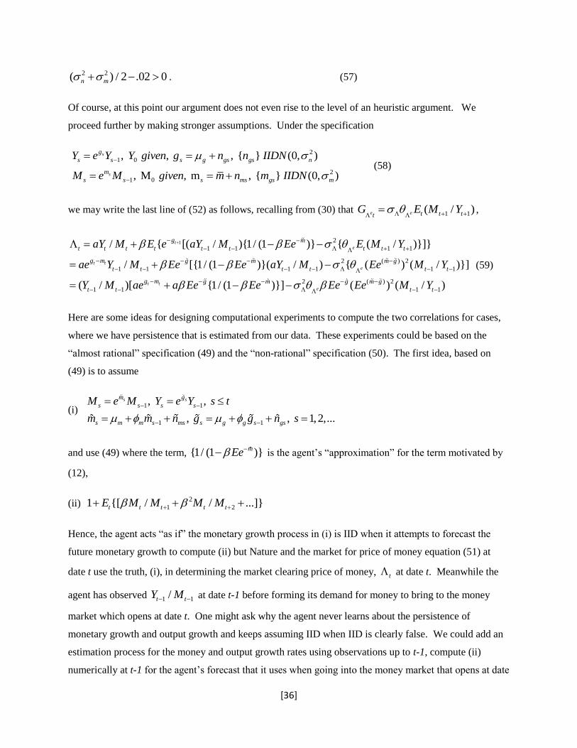
[36]

2 2( ) / 2 .02 0n m . (57)

Of course, at this point our argument does not even rise to the level of an heuristic argument. We

proceed further by making stronger assumptions. Under the specification

2

1 0

2

1 0

, , , { } (0, )

, M , m , { } (0, )

s

s

g

s s s g gs gs n

m

s s s ms gs m

Y e Y Y given g n n IIDN

M e M given m n m IIDN

(58)

we may write the last line of (52) as follows, recalling from (30) that 1 1( / )e e t t ttG E M Y

,

1 2

1 1 1 1

2 ( ) 2

1 1 1 1 1 1

1 1

/ { [( / ){1/ (1 )} { ( / )}]}

/ [{1/ (1 )}( / ) { ( ) ( / )}]

( / )[ {1/ (1 )}]

te

t te

t t

g m

t t t t t t t t t

g m g m m g

t t t t t t

g m g m

t t

aY M E e aY M Ee E M Y

ae Y M Ee Ee aY M Ee M Y

Y M ae a Ee Ee

2 ( ) 2

1 1( ) ( / )e

g m g

t tEe Ee M Y

(59)

Here are some ideas for designing computational experiments to compute the two correlations for cases,

where we have persistence that is estimated from our data. These experiments could be based on the

“almost rational” specification (49) and the “non-rational” specification (50). The first idea, based on

(49) is to assume

(i) 1 1

1 1

, ,

, , 1,2,...

s sm g

s s s s

s m m s ms s g g s gs

M e M Y e Y s t

m m n g g n s

and use (49) where the term, {1/ (1 )}mEe is the agent’s “approximation” for the term motivated by

(12),

(ii) 2

1 21 {[ / / ...]}t t t t tE M M M M

Hence, the agent acts “as if” the monetary growth process in (i) is IID when it attempts to forecast the

future monetary growth to compute (ii) but Nature and the market for price of money equation (51) at

date t use the truth, (i), in determining the market clearing price of money, t at date t. Meanwhile the

agent has observed 1 1/t tY M at date t-1 before forming its demand for money to bring to the money

market which opens at date t. One might ask why the agent never learns about the persistence of

monetary growth and output growth and keeps assuming IID when IID is clearly false. We could add an

estimation process for the money and output growth rates using observations up to t-1, compute (ii)

numerically at t-1 for the agent’s forecast that it uses when going into the money market that opens at date

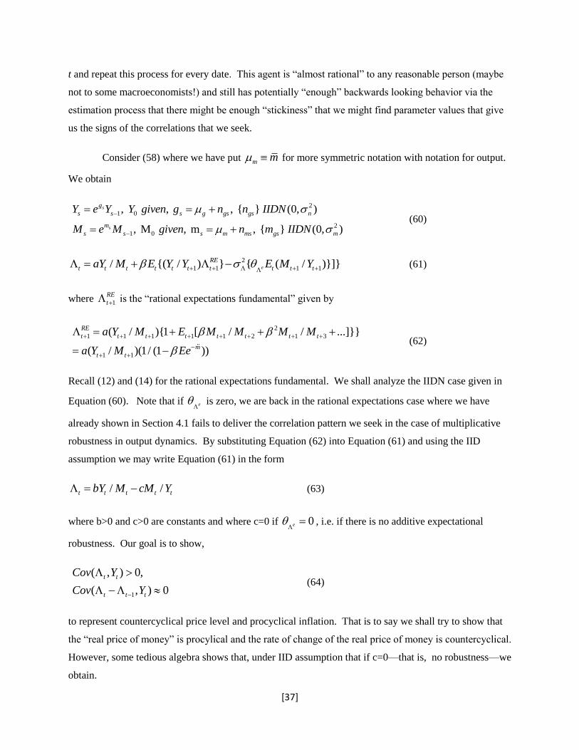
[37]

t and repeat this process for every date. This agent is “almost rational” to any reasonable person (maybe

not to some macroeconomists!) and still has potentially “enough” backwards looking behavior via the

estimation process that there might be enough “stickiness” that we might find parameter values that give

us the signs of the correlations that we seek.

Consider (58) where we have put m m for more symmetric notation with notation for output.

We obtain

2

1 0

2

1 0

, , , { } (0, )

, M , m , { } (0, )

s

s

g

s s s g gs gs n

m

s s s m ms gs m

Y e Y Y given g n n IIDN

M e M given n m IIDN

(60)

2

1 1 1 1/ {( / ) } { ( / )}]}e

RE

t t t t t t t t t taY M E Y Y E M Y (61)

where 1

RE

t is the “rational expectations fundamental” given by

2

1 1 1 1 1 2 1 3

1 1

( / ){1 [ / / ...]}}

( / )(1/ (1 ))

RE

t t t t t t t t

m

t t

a Y M E M M M M

a Y M Ee

(62)

Recall (12) and (14) for the rational expectations fundamental. We shall analyze the IIDN case given in

Equation (60). Note that if e

is zero, we are back in the rational expectations case where we have

already shown in Section 4.1 fails to deliver the correlation pattern we seek in the case of multiplicative

robustness in output dynamics. By substituting Equation (62) into Equation (61) and using the IID

assumption we may write Equation (61) in the form

/ /t t t t tbY M cM Y (63)

where b>0 and c>0 are constants and where c=0 if 0e , i.e. if there is no additive expectational

robustness. Our goal is to show,

1

( , ) 0,

( , ) 0

t t

t t t

Cov Y

Cov Y

(64)

to represent countercyclical price level and procyclical inflation. That is to say we shall try to show that

the “real price of money” is procylical and the rate of change of the real price of money is countercyclical.

However, some tedious algebra shows that, under IID assumption that if c=0—that is, no robustness—we

obtain.

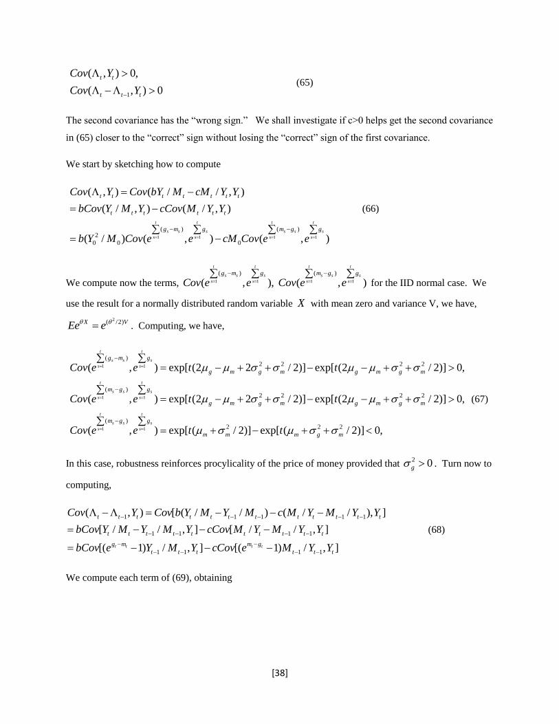
[38]

1

( , ) 0,

( , ) 0

t t

t t t

Cov Y

Cov Y

(65)

The second covariance has the “wrong sign.” We shall investigate if c>0 helps get the second covariance

in (65) closer to the “correct” sign without losing the “correct” sign of the first covariance.

We start by sketching how to compute

1 1 1 1

( ) ( )2

0 0 0

( , ) ( / / , )

( / , ) ( / , )

( / ) ( , ) ( , )

t t t t

s s s s s s

s s s s

t t t t t t t

t t t t t t

g m g m g g

Cov Y Cov bY M cM Y Y

bCov Y M Y cCov M Y Y

b Y M Cov e e cM Cov e e

(66)

We compute now the terms, 1 1 1 1

( ) ( )

( , ), ( , )

t t t t

s s s s s s

s s s s

g m g m g g

Cov e e Cov e e

for the IID normal case. We

use the result for a normally distributed random variable X with mean zero and variance V, we have,

2( /2)X VEe e . Computing, we have,

1 1

1 1

1 1

( )2 2 2 2

( )2 2 2 2

( )

( , ) exp[ (2 2 / 2)] exp[ (2 / 2)] 0,

( , ) exp[ (2 2 / 2)] exp[ (2 / 2)] 0,

( , ) exp[ (

t t

s s s

s s

t t

s s s

s s

t t

s s s

s s

g m g

g m g m g m g m

m g g

g m g m g m g m

m g g

m

Cov e e t t

Cov e e t t

Cov e e t

2 2 2/ 2)] exp[ ( / 2)] 0, m m g mt

(67)

In this case, robustness reinforces procylicality of the price of money provided that 2 0g . Turn now to

computing,

1 1 1 1 1

1 1 1 1

1 1 1 1

( , ) [ ( / / ) ( / / ), ]

[ / / , ] [ / / , ]

[( 1) / , ] [( 1) / , ]t t t t

t t t t t t t t t t t t

t t t t t t t t t t

g m m g

t t t t t t

Cov Y Cov b Y M Y M c M Y M Y Y

bCov Y M Y M Y cCov M Y M Y Y

bCov e Y M Y cCov e M Y Y

(68)

We compute each term of (69), obtaining

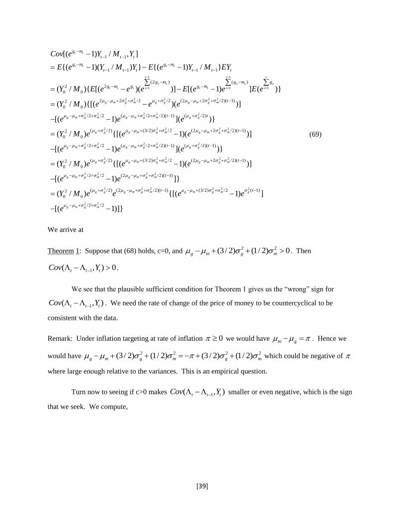
[39]

1 1

1 1 1

2 2

1 1

1 1 1 1

(2 ) ( )22

0 0

2 2 /22

0 0

[( 1) / , ]

{( 1)( / ) } {( 1) / }

( / ){ [( )( )] [( 1) ] ( )}

( / ){[(

t t

t t t t

t t t

s s s s s

t t t s t t s s

g m g m g

g m

t t t

g m g m

t t t t t t

g m g m gg m g g m

Cov e Y M Y

E e Y M Y E e Y M EY

Y M E e e e E e e E e

Y M e e

2 2 2

2 2 2 2 2

2 2 2 2 2

2 2

/2 (2 2 /2)( 1)

/2 /2 ( /2 /2)( 1) ( /2)

( /2) (3/2) /2 (2 2 /2)( 1)2

0 0

/2 /2 (

)( )]

[( 1) ]( )}

( / ) {[( 1)( )]

[( 1)

g g m g m

g m g m g m g m g g

g g g m g m g m g m

g m g m

t

t t

t

e

e e e

Y M e e e

e e

2 2 2

2 2 2 2 2

2 2 2 2

2 2

/2 /2)( 1) ( /2)( 1)

( /2) (3/2) /2 (2 2 /2)( 1)2

0 0

/2 /2 (2 /2)( 1)

( /2) (22

0 0

]( )}

( / ) {[( 1)( )]

[( 1) ]}

( / )

g m g m g g

g g g m g m g m g m

g m g m g m g m

g g g m g

t t

t

t

e

Y M e e e

e e

Y M e e

2 2 2 2

2 2

/2)( 1) (3/2) /2 ( 1)

/2 /2

{[( 1) ]

[( 1)]}

m g m g m g

g m g m

t te e

e

(69)

We arrive at

Theorem 1: Suppose that (68) holds, c=0, and 2 2(3 / 2) (1/ 2) 0g m g m . Then

1( , ) 0t t tCov Y .

We see that the plausible sufficient condition for Theorem 1 gives us the “wrong” sign for

1( , )t t tCov Y . We need the rate of change of the price of money to be countercyclical to be

consistent with the data.

Remark: Under inflation targeting at rate of inflation 0 we would have m g . Hence we

would have 2 2 2 2(3 / 2) (1/ 2) (3 / 2) (1/ 2)g m g m g m which could be negative of

where large enough relative to the variances. This is an empirical question.

Turn now to seeing if c>0 makes 1( , )t t tCov Y smaller or even negative, which is the sign

that we seek. We compute,

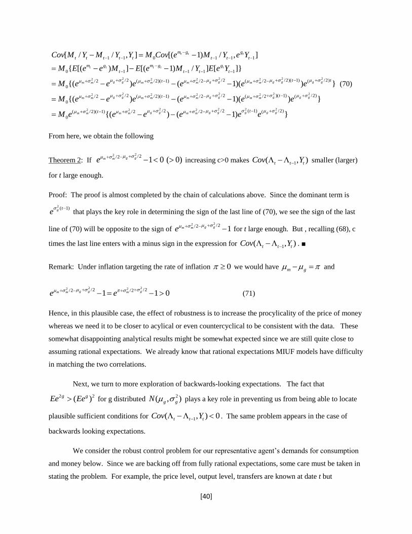
[40]

2 2 22 2 2 2

1 1 0 1 1 1

0 1 1 1 1

/2 /2 /2)(/2 ( /2)( 1) /2 ( /2

0

[ / / , ] [( 1) / , ]

{ [( ) ] [( 1) / ] [ ]}

{( ) ( 1)(

t t t

t t t t t

g g g g g gm m m m m m m m

m g g

t t t t t t t t

m g m g g

t t t t

tt

Cov M Y M Y Y M Cov e M Y e Y

M E e e M E e M Y E e Y

M e e e e e

2

2 2 2 22 2 2 2

2 2 2 22 2 2

1) /2)(

/2 /2 )( 1) /2)/2 ( /2)( 1) /2 ( /2 (

0

/2 /2 ( 1) /2)( /2)( 1) /2 /2 (

0

) }

{( ) ( 1)( ) }

{( ) ( 1) }

g g

g g g g g g gm m m m m m m m

g g g g g g gm m m m m m

t

tt

tt

e

M e e e e e e

M e e e e e e

(70)

From here, we obtain the following

Theorem 2: If 22 /2/2

1 0 ( 0)g gm me

increasing c>0 makes 1( , )t t tCov Y smaller (larger)

for t large enough.

Proof: The proof is almost completed by the chain of calculations above. Since the dominant term is

2 ( 1)g te

that plays the key role in determining the sign of the last line of (70), we see the sign of the last

line of (70) will be opposite to the sign of 22 /2/2

1g gm me

for t large enough. But , recalling (68), c

times the last line enters with a minus sign in the expression for 1( , )t t tCov Y . ■

Remark: Under inflation targeting the rate of inflation 0 we would have m g and

2 22 2/2 /2/2 /21 1 0g g gm m me e

(71)

Hence, in this plausible case, the effect of robustness is to increase the procylicality of the price of money

whereas we need it to be closer to acylical or even countercyclical to be consistent with the data. These

somewhat disappointing analytical results might be somewhat expected since we are still quite close to

assuming rational expectations. We already know that rational expectations MIUF models have difficulty

in matching the two correlations.

Next, we turn to more exploration of backwards-looking expectations. The fact that

2 2( )g gEe Ee for g distributed 2( , )g gN plays a key role in preventing us from being able to locate

plausible sufficient conditions for 1( , ) 0t t tCov Y . The same problem appears in the case of

backwards looking expectations.

We consider the robust control problem for our representative agent’s demands for consumption

and money below. Since we are backing off from fully rational expectations, some care must be taken in

stating the problem. For example, the price level, output level, transfers are known at date t but

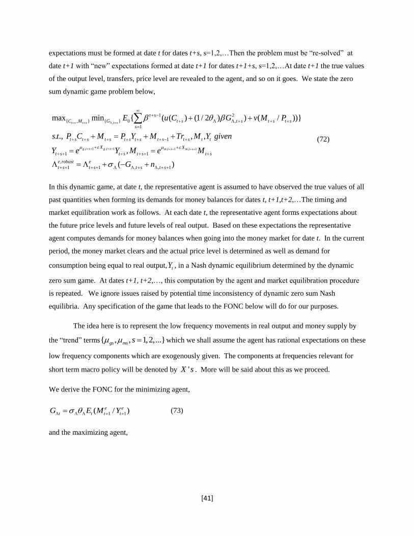
[41]

expectations must be formed at date t for dates t+s, s=1,2,…Then the problem must be “re-solved” at

date t+1 with “new” expectations formed at date t+1 for dates t+1+s, s=1,2,…At date t+1 the true values

of the output level, transfers, price level are revealed to the agent, and so on it goes. We state the zero

sum dynamic game problem below,

,

, 1 , 1 , 1 , 1

1 2

{ , } { } 0 ,

1

1

1 1

1

max min { ( ( ) (1/ 2 ) ) ( / ))}

. ., , ,

,

t s t s t s

g t s g t s m t s m t s

t s

C M G t s t s t s t s

s

t s t s t s t s t s t s t s t t

X X

t s t s t s t s

e

t s

E u C G v M P

s t P C M P Y M Tr M Y given

Y e Y M e M

,

1 , , 1( )robust e

t s t s t sG n

(72)

In this dynamic game, at date t, the representative agent is assumed to have observed the true values of all

past quantities when forming its demands for money balances for dates t, t+1,t+2,…The timing and

market equilibration work as follows. At each date t, the representative agent forms expectations about

the future price levels and future levels of real output. Based on these expectations the representative

agent computes demands for money balances when going into the money market for date t. In the current

period, the money market clears and the actual price level is determined as well as demand for

consumption being equal to real output, tY , in a Nash dynamic equilibrium determined by the dynamic

zero sum game. At dates t+1, t+2,…, this computation by the agent and market equilibration procedure

is repeated. We ignore issues raised by potential time inconsistency of dynamic zero sum Nash

equilibria. Any specification of the game that leads to the FONC below will do for our purposes.

The idea here is to represent the low frequency movements in real output and money supply by

the “trend” terms{ , , 1,2,...}gs ms s which we shall assume the agent has rational expectations on these

low frequency components which are exogenously given. The components at frequencies relevant for

short term macro policy will be denoted by 'X s . More will be said about this as we proceed.

We derive the FONC for the minimizing agent,

1 1( / )e e

t t t tG E M Y (73)

and the maximizing agent,

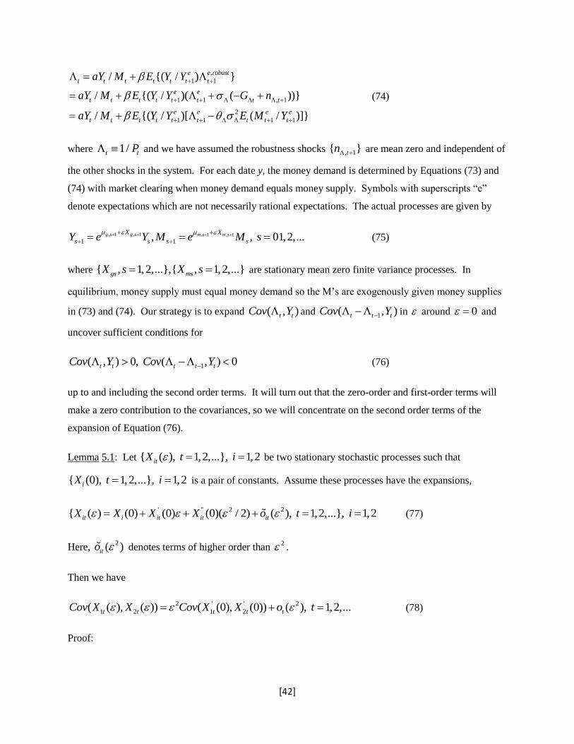
[42]

,

1 1

1 1 , 1

2

1 1 1 1

/ {( / ) }

/ {( / )( ( ))}

/ {( / )[ ( / )]}

e e robust

t t t t t t t

e e

t t t t t t t t

e e e e

t t t t t t t t t

aY M E Y Y

aY M E Y Y G n

aY M E Y Y E M Y

(74)

where 1/t tP and we have assumed the robustness shocks , 1{ }tn are mean zero and independent of

the other shocks in the system. For each date y, the money demand is determined by Equations (73) and

(74) with market clearing when money demand equals money supply. Symbols with superscripts “e”

denote expectations which are not necessarily rational expectations. The actual processes are given by

, 1 , 1 , 1 , 1

1 1, , 01,2,...g s g s m s m sX X

s s s sY e Y M e M s

(75)

where { , 1,2,...},{ , 1,2,...}gs msX s X s are stationary mean zero finite variance processes. In

equilibrium, money supply must equal money demand so the M’s are exogenously given money supplies

in (73) and (74). Our strategy is to expand ( , )t tCov Y and 1( , )t t tCov Y in around 0 and

uncover sufficient conditions for

1( , ) 0, ( , ) 0t t t t tCov Y Cov Y (76)

up to and including the second order terms. It will turn out that the zero-order and first-order terms will

make a zero contribution to the covariances, so we will concentrate on the second order terms of the

expansion of Equation (76).

Lemma 5.1: Let { ( ), 1,2,...}, 1,2itX t i be two stationary stochastic processes such that

{ (0), 1,2,...}, 1,2iX t i is a pair of constants. Assume these processes have the expansions,

' '' 2 2{ ( ) (0) (0) (0)( / 2) ( ), 1,2,...}, 1,2it i it it itX X X X o t i (77)

Here, 2( )ito denotes terms of higher order than

2 .

Then we have

2 ' ' 2

1 2 1 2( ( ), ( )) ( (0), (0)) ( ), 1,2,...t t t t tCov X X Cov X X o t (78)

Proof:

[43]

1 2

' '' 2 2 ' '' 2 2

1 1 1 1 2 2 2 2

' '' 2 2 ' '' 2 2

1 1 1 2 2 2

' '

1 2

( ( ), ( ))

( (0) (0) (0)( / 2) ( ), (0) (0) (0)( / 2) ( ))

( (0) (0)( / 2) ( ), (0) (0)( / 2) ( ))

( (0) , (0) ) (

t t

t t t t t t

t t t t t t

t t t

Cov X X

Cov X X X o X X X o

Cov X X o X X o

Cov X X o

2

2 ' ' 2

1 2

)

( (0), (0)) ( ), 1,2,...t t tCov X X o t

(79)

■

Since our representative agent is assumed to face an environment where low frequency components are

determined by long term trend forces that are independent of short term macro policies, a natural way to

express this environment for real output dynamics is to assume, for example, in Equation (75),

0

1

exp( ( )), 1,2,...t

t gs gs

s

Y Y X t

(80)

where the stochastic process { , 1,2,...}gsX s represents the total effect of shorter term fluctuations from

previous periods up to date t. The term 0 is intended to capture the idea that the fluctuations at the

business cycle frequencies are small relative to the lower frequency trend components, { }gt of

institutions, technical progress, demographics, etc. that determine the trends in real output dynamics. We

specify the dynamics of money supply similarly. More specifically, to keep things simple but preserve

our stance, we assume,

Assumption 5.1:

, 1 , 1

, 11 , 1

0 0

( 1) ( 1)

1 0 1 0

( 1)( )

1 0 0

, , 1,2,...

,

( ) ( ) , 0,1,2,...

0

g gt m mt

e eg g t m m t

eeg m tt t

t X t X

t t

t X t Xe e

t t

t XXe

t

m g

Y Y e M M e t

Y Y e M M e

e e t

(81)

More will be said about the actual specifications of the processes in (81) as we work through special cases

below. Note that Assumption 5.1 imposes rational expectations on long term trends in the middle two

lines. The last line of Assumption 5.1 is the assumption of an inflation target of zero. We analyze this

case here for simplicity and discuss more general inflation targeting later. We write Equation (82) below

for general inflation targeting at a constant rate of inflation and at a zero rate so one can see what

modification will be needed. Under Assumption 5.1 we may write

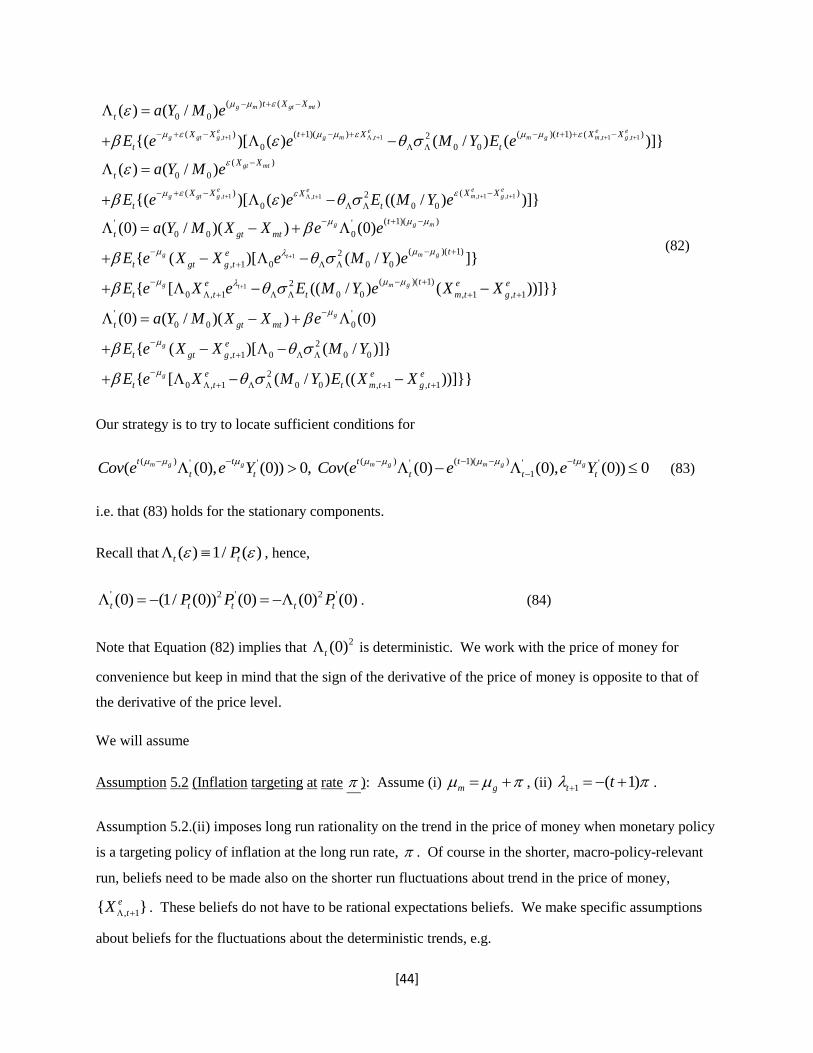
[44]

, 1 , 1 , 1 , 1

, 1

( ) ( )

0 0

( ) ( 1)( ) ( )( 1) ( )2

0 0 0

( )

0 0

( )

0

( ) ( / )

{( )[ ( ) ( / ) ( )]}

( ) ( / )

{( )[ ( )

g m gt mt

e e e eg gt g t g m t m g m t g t

gt mt

eg gt g t

t X X

t

X X t X t X X

t t

X X

t

X X X

t

a Y M e

E e e M Y E e

a Y M e

E e e

, 1 , 1, 1

1

1

( )2

0 0

( 1)( )' '

0 0 0

( )( 1)2

, 1 0 0 0

( )(2

0 , 1 0 0

(( / ) )]}

(0) ( / )( ) (0)

{ ( )[ ( / ) ]}

{ [ (( / )

e eem t g tt

g g m

g m gt

g m gt

X X

t

t

t gt mt

te

t gt g t

te

t t t

E M Y e

a Y M X X e e

E e X X e M Y e

E e X e E M Y e

1)

, 1 , 1

' '

0 0 0

2

, 1 0 0 0

2

0 , 1 0 0 , 1 , 1

( ))]}}

(0) ( / )( ) (0)

{ ( )[ ( / )]}

{ [ ( / ) (( ))]}}

g

g

g

e e

m t g t

t gt mt

e

t gt g t

e e e

t t t m t g t

X X

a Y M X X e

E e X X M Y

E e X M Y E X X

(82)

Our strategy is to try to locate sufficient conditions for

( ) ( ) ( 1)( )' ' ' ' '

1( (0), (0)) 0, ( (0) (0), (0)) 0m g g m g m g gt t t t t

t t t t tCov e e Y Cov e e e Y

(83)

i.e. that (83) holds for the stationary components.

Recall that ( ) 1/ ( )t tP , hence,

' 2 ' 2 '(0) (1/ (0)) (0) (0) (0)t t t t tP P P . (84)

Note that Equation (82) implies that 2(0)t is deterministic. We work with the price of money for

convenience but keep in mind that the sign of the derivative of the price of money is opposite to that of

the derivative of the price level.

We will assume

Assumption 5.2 (Inflation targeting at rate ): Assume (i) m g , (ii) 1 ( 1)t t .

Assumption 5.2.(ii) imposes long run rationality on the trend in the price of money when monetary policy

is a targeting policy of inflation at the long run rate, . Of course in the shorter, macro-policy-relevant

run, beliefs need to be made also on the shorter run fluctuations about trend in the price of money,

, 1{ }e

tX . These beliefs do not have to be rational expectations beliefs. We make specific assumptions

about beliefs for the fluctuations about the deterministic trends, e.g.

[45]

Assumption 5.3: , 1 , 1 , 1 , 1, e e

t g t g t t m t m tE X X E X X

Assumption 5.4: , 1 , 1 , 10 , 0,1,2,...

0 , 1,2,...

e e e

g t m t t

gt mt

EX EX EX t

EX EX t

Under Assumptions 5.3, 5.4, and Assumption 5.2 with 0 allows us to compute (noting that the

constant term, '

0 (0)ge

, from (82) cancels out in the covariance),

' '

0 0

2

0 0 0 , 1

2

0 , 1 0 0 , 1 , 1

( (0), (0)) { [ ( / )( )

{ ( ( / ))}( )

{ [ ( / )( )]}]}

g

g

g

t

t t gt gt mt

gt g t

e

t m t g t

Cov e Y E X a Y M X X

e M Y X X

e X M Y X X

(85)

' ' '

1 0 0

2

0 0 0 , 1

2

0 , 1 0 0 , 1 , 1

( (0) (0), (0)) { [ ( / )( )

{ ( ( / ))}( )

{ [ ( / )( )]}]}

g

g

g

t

t t t gt gt mt

gt g t

e

t m t g t

Cov e Y E X a Y M dX dX

e M Y dX dX

e dX M Y dX dX

(86)

where for any random variable 1, , 1,2,...t t t tZ dZ Z Z t .

Our task now is to locate sufficient conditions for

' ' ' ' '

1( (0), (0)) 0, ( (0) (0), (0)) 0g gt t

t t t t tCov e Y Cov e Y

(87)

Note that one needs to “take out” the exponential growth factors to render the processes stationary so that

unconditional covariances are meaningful.

We now specify the X processes in more detail as VAR’s. For convenience label as follows, 1=g,

2=m, 3= . Then write

3

, 1 , 1

1

1 1

1 1 0 0

, 1,2,3, 1,2,...

, { , 1,2,...}, (0, )

( ) ( ) , 1,2,..., ( )

i t ij jt i t

j

t t t t n

T T T T

t t t t n

X a X n i t

X AX n n t IID

E X X AE X X A t E X X given

(88)

We now have quite a bit of flexibility to specify stochastic processes for the shorter run fluctuations about

trend to achieve the objective in (87). Note that a small or zero covariance for the rate of change of the

[46]

price of money is roughly consistent with the data. The real issue will be whether our specifications that

achieve the matching of the two correlations in (87) are plausible from a macroeconomic view point.

The reader may object to our specification of expectations on 1

e

t because of lack of rationality.

In other words, there should be, at least, some self-consistency restrictions if one does not go all the way

to requiring rational expectations. We assume

Assumption 5.5: 1 0 0( 1)( ), e

t m gt

Assumption 5.5 requires that the expectations on the trend component and the constant term be rational.

Note that we have already assumed rational expectations on the constant term 0 in (81) and used it in

(82) and what follows. We make the formal assumption on rational expectations on the constant term

here. What other properties might be plausible to impose on the shorter term components of inflation

expectations, , 1{ , 0,1,2,...}e

t tE X t ? The Cleveland Fed produces detailed estimates of the public’s

inflation expectations.17

Let us examine a very special case where shorter term movements in inflation expectations may

produce the sign pattern in the two correlations that we seek. Shorten notation for conditional

expectations by writing,

, 1 , 1| , 1 , 1| , 1 , 1|, , e e e e e e

t g t g t t t m t m t t t t t tE X X E X X E X X . (89)

Assumption 5.6: , 1|0, , 0e

m g g t t gtX X , i.e. zero targeted inflation by long run monetary

policy, “quasi”-rational expectations on output dynamics, and zero robustness.

Then, under Assumption 5.6, we may write,

, 1( )

0 0 0

' '

0 0 0 , 1| 0

' '

1 0 0 , 1 , 1 0 , 1| , | 1

( ) ( / ) ( )

(0) ( / )( ) (0) (0)

(0) (0) ( / )( ( ) (0)[ ]

egt mt g t

g g

g

X X X

t t

e

t gt mt t t

e e

t t gt g t mt m t t t t t

a Y M e e E e

a Y M X X e X e

a Y M X X X X e X X

(90)

From (90) we have,

17

See Haubrich, Pennacchi, and Ritchken (2012) for a more detailed discussion regarding heterogeneity in the inflation expectations formation.

[47]

'

0 0 0 , 1|

' '

1 0 0 0 , 1|

( (0), ) ( / ) [( ) ] (0) [ ]

( (0) (0), ) ( / ) [( ) ] (0) [ ]

g

g

e

t gt gt mt gt t t gt

e

t t gt gt mt gt t t gt

Cov X a Y M E X X X e E X X

Cov X a Y M E dX dX X e E dX X

(91)

where we have used the “d” notation to denote first differences. Recall that we are after sufficient

conditions of macro-economic plausibility for the first covariance to be positive and the second to be

negative or zero or close to zero.

We have already argued that it is plausible that [( ) ] 0gt mt gtE X X X . Based on Webb, it

seems quite plausible that the covariance of contemporaneous inflation expectations with real output

fluctuations is non-negative; that is, , 1|{ } 0e

t t gtE X X . Note that this covariance could be negative and

we would still have the contemporaneous covariance of the macro-frequency fluctuations in the price of

money with the macro-frequency fluctuations in real output be positive. How plausible is it that the

covariance, , 1|

e

t t gtEdX X , be negative? Webb’s arguments are based on quotes from Mitchell (Webb,

(2003), pages 70 and 71) in which the description is that as real output rises above trend, the rate of

change of inflation will tend to rise above trend. Hence, the “price of money” will tend to fall. This could

be interpreted as supporting the plausibility of , 1|{ } 0e

t t gtE dX X .

The following Lemma about computing covariances from VAR’s will be used in what follows

Lemma 5.2: Consider the general VAR with constant coefficients

, 1 , 1

1

1 1

1 1 0 0

, 1,2,..., , 1,2,...

, { , 1,2,...}, (0, )

( ) ( ) , 1,2,..., ( )

N

i t ij jt i t

j

t t t t n

T T T T

t t t t n

X a X n i N t

X AX n n t IID

E X X AE X X A t E X X given

(92)

where the VAR is written in matrix form in the second line and the dynamics of the NxN covariance

matrix are given in the third line. Assume the initial condition 0 0( )TE X X for the variance matrix is at the

stationary solution of the last line of (92). Consider the linear combination with constant coefficients

1

, 1,2,...I

t i it

i

Z X t

(93)

Then the unconditional covariances of Z and its first difference with any of the X’s, say, 1tX are given by

[48]

1 1

1

1 1 1 , 1 1 , 1 1

1 1 1

1 1 1 , 1

1

1 1

1

11 1 1

( , ) ( )

( , ) ( ) [ ( )]

( , ) ( , )

( , ) ( , )

(1 ) ( , ) ( , )

N

t t i it t

i

N N N

t t t i it t i i t j j t t

i i j

N

t t j t j t

j

N

t t j t jt

j

t t j t jt

Cov Z X E X X

Cov Z Z X E X X E X a X n

Cov Z X a Cov Z X

Cov Z X a Cov Z X

a Cov Z X a Cov Z X

2

N

j

(94)

Proof: The first line of the Lemma follows because Z and the X’s all have mean zero and we start with

initial conditions having mean zero. The second and third lines follow by simple computation. The

fourth line follows from the stationarity assumption. The fifth line is obvious. ■

Note that if the VAR is diagonal, this simple Lemma implies that it is not possible for the signs of

1( , )t tCov Z X and 1 1( , )t t tCov Z Z X to be different. Hence we must work with a non-diagonal VAR

if we want to match the signs of the two covariances.

We apply Lemma 5.2 to different cases of Equations (85) and (86). We start with the simplest

possible case of no robustness, 0 , deterministic money supply, i.e. 0mtX , and drop irrelevant

constants to obtain

' '

0 0 0 , 1|

2

1 1 1 2 3 1 3 1 1 3 1 3

1 0 0 3 0 0 0

( (0), (0)) ( / ) { ( )} (0) ( )

{ ( )} ( ) ( )

( / ), (0) ( / ) / (1 )

g g

g g g

t e

t t gt gt mt gt t t

t t t t t t t t

Cov e Y a Y M E X X X e E X X

E X X X E X X EX E X X

a Y M e e a Y M e

(95)

where the last line of Equation (95) follows from the assumption of rationality of inflation expectations on

the constant term 0 0 0(0) ( / ) / (1 )ga Y M e

. The second covariance is computed as follows,

[49]

' ' '

1

0 0 , 1 0 , 1| , | 1

1 1 1 1, 1 3 1 3 3, 1

2

1 1 1 1 1, 1 3 1 3 3 1 3, 1

1 11 1

( (0) (0), (0))

( / ) { ( )} (0) ( ( )

{ ( )} ( ( )

( ) ( ) ( )

(1 )

g

g

t

t t t

e e

gt gt g t gt t t t t

t t t t t t

t t t t t t t

Cov e Y

a Y M E X X X e E X X X

E X X X E X X X

EX E X X E X X E X X

a EX

2

1 13 3, 1 1, 1 3 1 3 3 1 3, 1

2 2

1 11 1 1 13 3 1 3 1 3 3 11 1, 3, 1 3 13 3, 1

2 2

11 1 1 3 1 3 1 13 1 3 3 13 3

( ) ( ) ( )

(1 ) ( ) ( ) ( )

(1 ){ ( )} ( )

t t t t t t t

t t t t t t t t

t t t t t t

a E X X E X X E X X

a EX a E X X E X X a E X X a EX

a EX E X X a E X X a EX

(96)

Stationarity was used in the computation of equations (95) and (96). Note that the first term of the last

line of Equation (95) has the same sign as ' '( (0), (0))gt

t tCov e Y

. As we have seen it is easy to locate

sufficient conditions so that ' '( (0), (0)) 0gt

t tCov e Y

. We argue that it is plausible that 13 0a ,

hence the term, 2

3 13 3 0ta EX reduces the size of ' ' '

1( (0) (0), (0))gt

t t tCov e Y

and may even turn

it negative when ' '( (0), (0)) 0gt

t tCov e Y

. The other “extra” term, 1 13 1 3( )t ta E X X , probably helps

our case because it is quite plausible that 1 3( ) 0t tE X X by the same type of argument used by Webb

where he quotes Mitchell, but for inflation expectations rather than inflation itself. Note that

3 1 2 1giff e

which will hold under plausible values in macro-economics, since is close to

one and g is small, for example, .02g . This suggests that terms weighted by 3 will play a bigger

role in determining conditions under which we obtain the sign pattern of the two covariances that we are

seeking. Ignoring the terms weighted by 1 we have

' '

3 1 3

' ' ' 2

1 3 11 1 3 13 3

( (0), (0))" " ( )

( (0) (0), (0))" " {(1 ) ( ) }

g

g

t

t t t t

t

t t t t t t

e Cov Y E X X

e Cov Y a E X X a EX

(97)

Since 1 3/ 0, 1 gas e

the sign pattern of the two covariances will be determined by the

terms on the RHS for ge

close to one. Note that the VAR and the covariances between the X’s are

independent of the weights 1 3, . Equation (97) suggests that if 1 3( ) 0t tE X X and if 2

13 3ta EX is large

enough then the first covariance will be positive and the second one will be negative. This is the sign

pattern that we seek. One final check that must be done is to compute closed form expressions for

1 3( )t tE X X and 2

13 3ta EX using Lemma 5.2 and equations (92)-(94) and locate a set of VAR coefficients

and conditions on the covariance matrix of the shocks to get the sign pattern that we want. After some

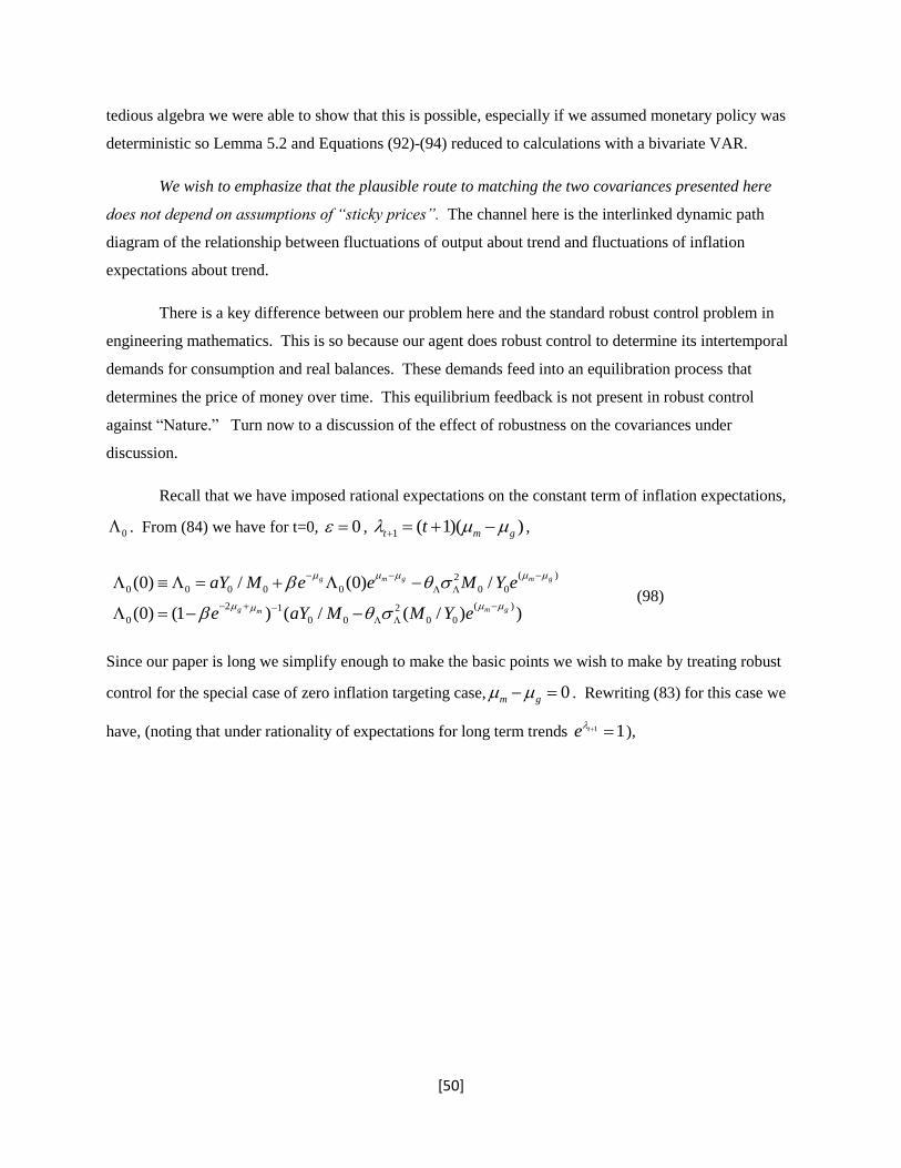
[50]

tedious algebra we were able to show that this is possible, especially if we assumed monetary policy was

deterministic so Lemma 5.2 and Equations (92)-(94) reduced to calculations with a bivariate VAR.

We wish to emphasize that the plausible route to matching the two covariances presented here

does not depend on assumptions of “sticky prices”. The channel here is the interlinked dynamic path

diagram of the relationship between fluctuations of output about trend and fluctuations of inflation

expectations about trend.

There is a key difference between our problem here and the standard robust control problem in

engineering mathematics. This is so because our agent does robust control to determine its intertemporal

demands for consumption and real balances. These demands feed into an equilibration process that

determines the price of money over time. This equilibrium feedback is not present in robust control

against “Nature.” Turn now to a discussion of the effect of robustness on the covariances under

discussion.

Recall that we have imposed rational expectations on the constant term of inflation expectations,

0 . From (84) we have for t=0, 0 , 1 ( 1)( )t m gt ,

( )2

0 0 0 0 0 0 0

2 ( )1 2

0 0 0 0 0

(0) / (0) /

(0) (1 ) ( / ( / ) )

g m g m g

g m gm

aY M e e M Y e

e aY M M Y e

(98)

Since our paper is long we simplify enough to make the basic points we wish to make by treating robust

control for the special case of zero inflation targeting case, 0m g . Rewriting (83) for this case we

have, (noting that under rationality of expectations for long term trends 1 1te ),

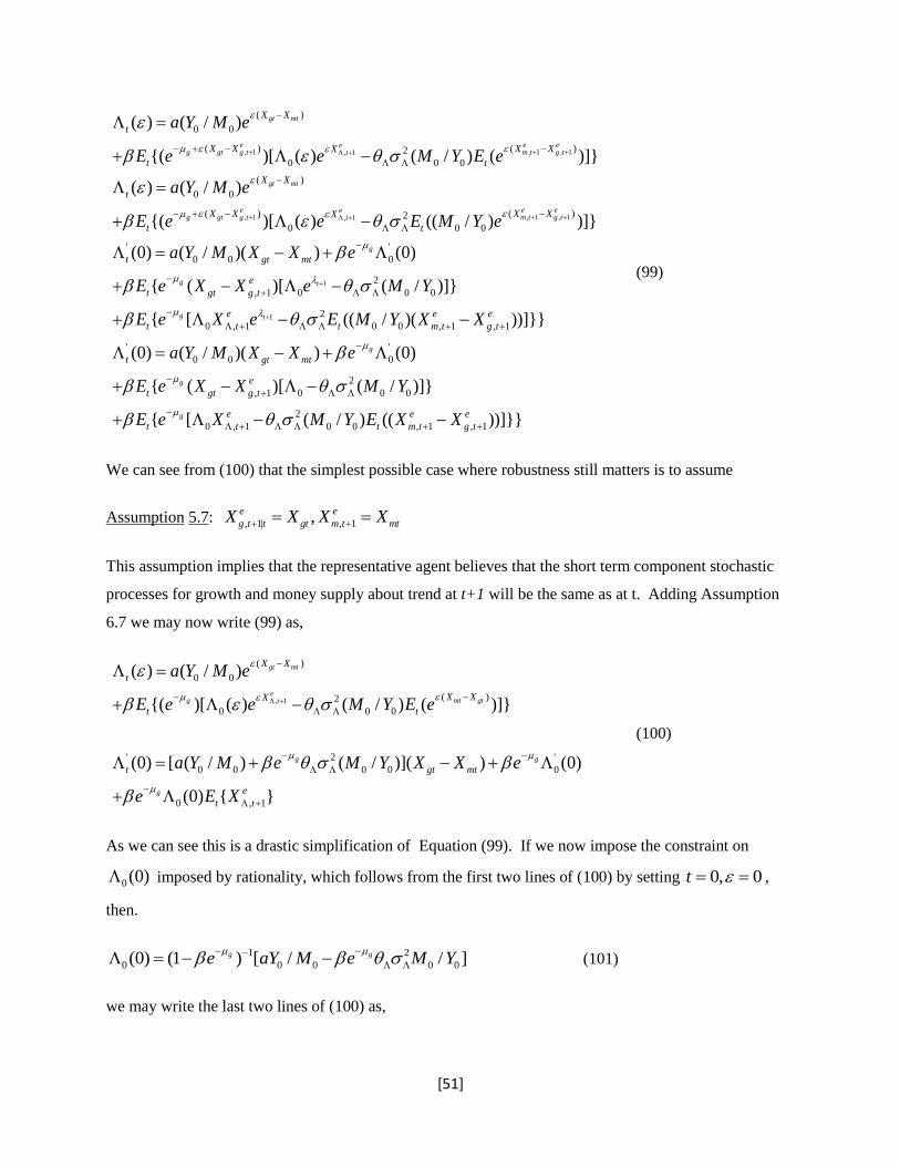
[51]

, 1 , 1 , 1, 1

, 1 , 1 ,, 1

( )

0 0

( ) ( )2

0 0 0

( )

0 0

( ) (2

0 0 0

( ) ( / )

{( )[ ( ) ( / ) ( )]}

( ) ( / )

{( )[ ( ) (( / )

gt mt

e e eeg gt g t m t g tt

gt mt

e eeg gt g t m t gt

X X

t

X X X XX

t t

X X

t

X X X XX

t t

a Y M e

E e e M Y E e

a Y M e

E e e E M Y e

1

1

1

)

' '

0 0 0

2

, 1 0 0 0

2

0 , 1 0 0 , 1 , 1

' '

0 0 0

)]}

(0) ( / )( ) (0)

{ ( )[ ( / )]}

{ [ (( / )( ))]}}

(0) ( / )( ) (0)

{ (

et

g

g t

g t

g

g

t gt mt

e

t gt g t

e e e

t t t m t g t

t gt mt

t gt

a Y M X X e

E e X X e M Y

E e X e E M Y X X

a Y M X X e

E e X

2

, 1 0 0 0

2

0 , 1 0 0 , 1 , 1

)[ ( / )]}

{ [ ( / ) (( ))]}}g

e

g t

e e e

t t t m t g t

X M Y

E e X M Y E X X

(99)

We can see from (100) that the simplest possible case where robustness still matters is to assume

Assumption 5.7: , 1| , 1,e e

g t t gt m t mtX X X X

This assumption implies that the representative agent believes that the short term component stochastic

processes for growth and money supply about trend at t+1 will be the same as at t. Adding Assumption

6.7 we may now write (99) as,

, 1

( )

0 0

( )2

0 0 0

' 2 '

0 0 0 0 0

0 , 1

( ) ( / )

{( )[ ( ) ( / ) ( )]}

(0) [ ( / ) ( / )]( ) (0)

(0) { }

gt mt

eg mt gtt

g g

g

X X

t

X XX

t t

t gt mt

e

t t

a Y M e

E e e M Y E e

a Y M e M Y X X e

e E X

(100)

As we can see this is a drastic simplification of Equation (99). If we now impose the constraint on

0 (0) imposed by rationality, which follows from the first two lines of (100) by setting 0, 0t ,

then.

1 2

0 0 0 0 0(0) (1 ) [ / / ]g ge aY M e M Y

(101)

we may write the last two lines of (100) as,

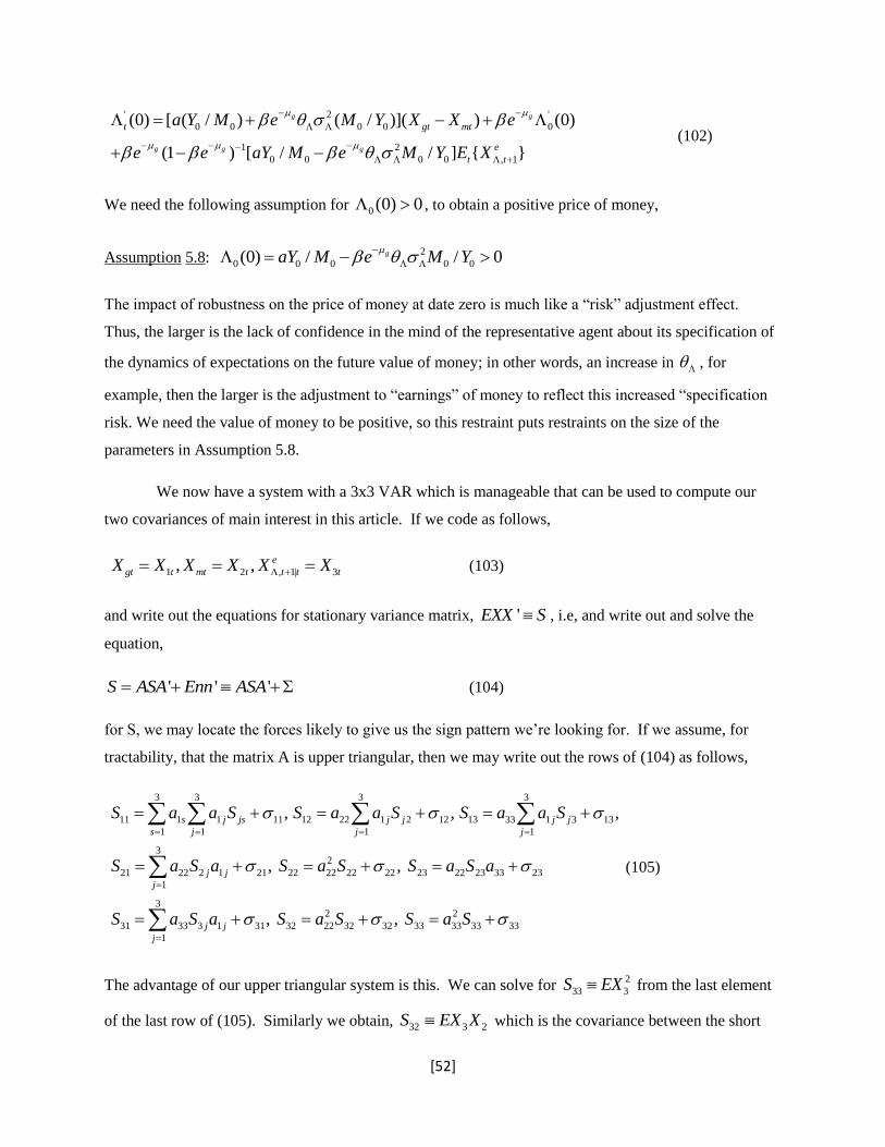
[52]

' 2 '

0 0 0 0 0

1 2

0 0 0 0 , 1

(0) [ ( / ) ( / )]( ) (0)

(1 ) [ / / ] { }

g g

g g g

t gt mt

e

t t

a Y M e M Y X X e

e e aY M e M Y E X

(102)

We need the following assumption for 0 (0) 0 , to obtain a positive price of money,

Assumption 5.8: 2

0 0 0 0 0(0) / / 0gaY M e M Y

The impact of robustness on the price of money at date zero is much like a “risk” adjustment effect.

Thus, the larger is the lack of confidence in the mind of the representative agent about its specification of

the dynamics of expectations on the future value of money; in other words, an increase in , for

example, then the larger is the adjustment to “earnings” of money to reflect this increased “specification

risk. We need the value of money to be positive, so this restraint puts restraints on the size of the

parameters in Assumption 5.8.

We now have a system with a 3x3 VAR which is manageable that can be used to compute our

two covariances of main interest in this article. If we code as follows,

1 2 , 1| 3, , e

gt t mt t t t tX X X X X X (103)

and write out the equations for stationary variance matrix, 'EXX S , i.e, and write out and solve the

equation,

' ' 'S ASA Enn ASA (104)

for S, we may locate the forces likely to give us the sign pattern we’re looking for. If we assume, for

tractability, that the matrix A is upper triangular, then we may write out the rows of (104) as follows,

3 3 3 3

11 1 1 11 12 22 1 2 12 13 33 1 3 13

1 1 1 1

32

21 22 2 1 21 22 22 22 22 23 22 23 33 23

1

32 2

31 33 3 1 31 32 22 32 32 33 33 33 33

1

, , ,

, ,

, ,

s j js j j j j

s j j j

j j

j

j j

j

S a a S S a a S S a a S

S a S a S a S S a S a

S a S a S a S S a S

(105)

The advantage of our upper triangular system is this. We can solve for 2

33 3S EX from the last element

of the last row of (105). Similarly we obtain, 32 3 2S EX X which is the covariance between the short

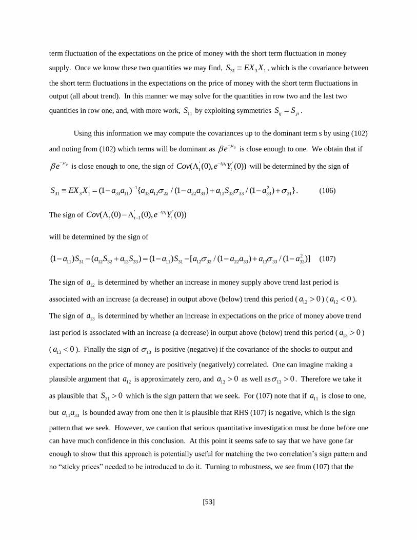
[53]

term fluctuation of the expectations on the price of money with the short term fluctuation in money

supply. Once we know these two quantities we may find, 31 3 1S EX X , which is the covariance between

the short term fluctuations in the expectations on the price of money with the short term fluctuations in

output (all about trend). In this manner we may solve for the quantities in row two and the last two

quantities in row one, and, with more work, 11S by exploiting symmetries ij jiS S .

Using this information we may compute the covariances up to the dominant term s by using (102)

and noting from (102) which terms will be dominant as ge

is close enough to one. We obtain that if

ge

is close enough to one, the sign of ' '( (0), (0))tt

t tCov e Y

will be determined by the sign of

1 2

31 3 1 33 11 33 12 22 22 33 13 33 33 33 31(1 ) { / (1 ) / (1 ) }S EX X a a a a a a a S a . (106)

The sign of ' ' '

1( (0) (0), (0))tt

t t tCov e Y

will be determined by the sign of

2

11 31 12 32 13 33 11 31 12 32 22 33 13 33 33(1 ) ( ) (1 ) [ / (1 ) / (1 )]a S a S a S a S a a a a a (107)

The sign of 12a is determined by whether an increase in money supply above trend last period is

associated with an increase (a decrease) in output above (below) trend this period ( 12 0a ) ( 12 0a ).

The sign of 13a is determined by whether an increase in expectations on the price of money above trend

last period is associated with an increase (a decrease) in output above (below) trend this period ( 13 0a )

( 13 0a ). Finally the sign of 13 is positive (negative) if the covariance of the shocks to output and

expectations on the price of money are positively (negatively) correlated. One can imagine making a

plausible argument that 12a is approximately zero, and 13 0a as well as 13 0 . Therefore we take it

as plausible that 31 0S which is the sign pattern that we seek. For (107) note that if 11a is close to one,

but 11 33a a is bounded away from one then it is plausible that RHS (107) is negative, which is the sign

pattern that we seek. However, we caution that serious quantitative investigation must be done before one

can have much confidence in this conclusion. At this point it seems safe to say that we have gone far

enough to show that this approach is potentially useful for matching the two correlation’s sign pattern and

no “sticky prices” needed to be introduced to do it. Turning to robustness, we see from (107) that the

[54]

main effect of robustness is to make the weights on the potentially dominant terms in the two covariances

smaller.

Of course we hasten to add that we have explored only one type of robustness. There may be

doubts in the mind of the representative agent about the specification of the dynamics of the VAR, about

the specification of the dynamics of output, even about trends, and so on.

We plan to do much more exploration of robustness effects in future research.

VI. Summary, Conclusions, and Suggestions for Future Research.

In this paper, we focus on the relationship between the price level and output at business cycle

frequencies. In particular, we are interested in characterizing two contemporaneous correlations: one is

the relationship between the price level and output and the other is the relationship between the inflation

rate and output. Because the inflation rate is the rate of change in the price level, the two facts convey

some underlying feature of the economy. In our case, the evidence consistently points to the price level

being countercyclical while the inflation rate is either procyclical or acyclical, depending on what method

we use to filter out the low-frequency component.

One thing we want to do is to develop a methodology to assess how much confidence we should

put in a “stylized fact” in a data disciplined way. In particular, our methodology is proposed as a data

disciplined way to assess the amount of uncertainty surrounding a “stylized fact” that takes into account,

not only estimation uncertainty but also model uncertainty. We illustrated our methodology with

assessing the uncertainty surrounding the stylized fact that the price level is countercyclical and the rate of

inflation is procyclical using U.S. data under two methods of filtering, e.g. difference stationary and trend

stationary (Nelson and Plosser (1982)). We found a rather high level of uncertainty in our illustrative

example. This should give pause to any theorist who wants to take a strong stand on which model or

theory to work with based on this particular “stylized fact.”

We see a promising and useful strand of future research that extends our methodology to

combined evidence from more than one country’s data. For example, the recent paper by

Konstantakopoulou et al. (2009), reports results on the correlation of filtered real output and filtered price

level and the correlation of real output and rate of inflation for many countries and several methods of

filtering out the low-frequency component. The countercylicality of the price level and the procyclicality

of the rate of inflation appear to be quite robust. However, one must be wary of thinking that that each

country’s evidence represents independent support of this particular “stylized fact”. This is so because

the business cycles of these 9 OECD countries are quite likely to be cross correlated and this cross

[55]

correlation must be taken into account when applying the bootstrap (Efron (1982), Efron and Tibshirani

(1986)) to compute the probability of the cyclicality pattern of price level and inflation under scrutiny

here.

The other contribution of this paper is to specify a model economy in which rational inattention is

present. Our goal is to quantitatively assess whether such a model can account for the observed pair of

correlations. The idea is pretty straightforward. The quantitative results indicate how important price

flexibility is to accounting for the negative correlation between the price level and output. In many model

economies, consumers are forward-looking, and when combined with persistent output shocks and central

bank operating rules, the quantitative analysis indicate that both the price level and the inflation rate are

countercyclical. Following the price expectations approach formulated in work by Brock and Hommes

(1997), we propose a model economy that can account for the pair of correlations observed; namely, that

in a difference-stationary setting, the price level is countercyclical and the inflation rate is acyclical. The

key is that price expectations are not rational, thereby imparting a price stickiness. Our numerical results

demonstrate that the by putting enough weight on backward-looking price expectations, we can induce

the phase shift in the price level that is consistent with the observed pattern of correlations. In a forward-

looking rational expectations model economy, we find that movements in the price level adjust

quantitatively so that the correlation between the price level and output and the inflation rate and output

are of the same sign. We consider a few modifications to the model economy, including money supply

rules, persistence in the output growth, and Hansen and Sargent-type preferences with uncertainty

regarding the economic environment. None appear to be promising frictional routes in terms of the

explaining countercyclical price level and either acyclical or procyclical inflation.

A more promising approach is the perturbation approach that we developed in the latter part of

section 5 which focused on fluctuations about trend where we assume rational expectations on the low-

frequency, or trend, dynamics but backed off from rational expectations on the business-cycle fluctuations

about trends. Not only does this approach introduce some novelty in the study of a well-known

“textbook” received MIUF model, it also helps us uncover forces that are not “sticky price” forces that are

consistent with stylized facts where it seems that a consensus has formed that “sticky prices” need to be

introduced in order to match these stylized facts. We illustrated this with the sign pattern of the two

correlations which form the main theme that runs through this entire paper.

Other directions of future research that we see as potentially fruitful are (i) developing extensions

of the simple methods of our paper towards something like a “sturdy” reporting of stylized facts rather in

the style of the “sturdy econometrics” advocated by Leamer (1994) and extension and adaptations of the

[56]

simple methods illustrated in our paper towards Bayesian Model Uncertainty methods of reporting better

measures of uncertainty when reporting a “stylized fact” than the more usual reporting of parameter

estimates with their corresponding standard errors.

[57]

Appendix

Proof Proposition 2:

Assume that the expected value of the product of the price level and output is constant over time. We

derive the following condition: [ ] {[ ][ ]}. After collecting terms and

simplifying, we can write this as [ ] [ ]

. With [ ] , it follows that [ ] iff .

Similarly, [ ] {[ ][ ]}. After collecting terms and simplifying, we

get [ ] [ ]( )

. With [ ] , and with , it follows that for [ ] .■

References

Aghion, Phillippe, Roman Frydman, Joseph Stiglitz, and Michael Woodford, eds., 2003, Knowledge,

Information, and Expectations in Modern Macroeconomics: In Honor of Edmund S. Phelps, Princeton

University Press: Princeton.

Anderson, Evan W., William A. Brock, Lars Peter Hansen, and Alan Sanstad, 2014. “Robust Analytical

and Computational Explorations of Coupled Economic-Climate Models with Carbon-Climate Response,”

RDCEP Working Paper 13-05.

Ball, Laurence and N. Gregory Mankiw, 1995. “A Sticky-Price Manifesto,” Carnegie-Rochester Series

on Public Policy, 41(1), 127-151.

Chadha, Bankim and Eswar Prasad, 1994. “Are Prices Countercyclical: Evidence from the G-7,” Journal

of Monetary Economics, 34: 239-57.

Blanchard, Olivier and Mark Watson, 1986. “Are All Business Cycles Alike?” Continuity and Change in

the American Business Cycle, Robert Gordon, ed., Chicago,IL : National Bureau of Economic Research

and University of Chicago Press.

Berkowitz, Jeremy and Lutz Kilian, 2000, “Recent Developments in Bootstrapping Time Series,”

Econometric Reviews, 19(1), 1-48.

Branch, William A. and George W. Evans, 2011, “Monetary Policy and Heterogeneous Expectations,”

Economic Theory, 47, 365-393.

Brock, William A., Steven N. Durlauf, and Kenneth D. West, 2003. “Policy Evaluation in Uncertain

Economic Environments,” Brookings Papers on Economic Activity, issue 1, 235-301.

______ , 2007. “Model Uncertainty and Policy Evaluation,” Journal of Econometrics, 136(2), 629-664.

Brock, William A. and Cars Hommes, 1997. “A Rational Route to Randomness,” Econometrica , 65:5,

1059-95.

Brock, William, Steven Durlauf and Giacoma Rondina, G, 2013, “Design Limits and Dynamic Policy

[58]

Analysis,” Journal of Economic Dynamics and Control, available on line, July 26, 2013.

Burdett, Kenneth and Kenneth L. Judd, 1983. “Equilibrium Price Dispersion,” Econometrica, 51(4), 955-

969.

Cooley, Thomas, F. and Lee E. Ohanian, 1991. “The Cyclical Behavior of Prices,” Journal of Monetary

Economics, 28(1), 25-60.

De Grauwe, Paul, 2011, “Animal Sprits and Monetary Policy,” Economic Theory, 47, 423-457.

den Haan, Wouter, 2000, “The Comovement Between Output and Prices,” Journal of Monetary

Economics, 46, 3-30.

Efron, Bradley, 1982, The Jacknife, The Bootstrap, and Other Resampling Plans, (Society for Industrial

and Applied Mathematics, Philadelphia)

Efron, Bradley and Tibshirani, Robert, 1986, “Bootstrap Methods for Standard Errors, Confidence

Intervals and Other Measures of Statistical Accuracy,” Statistical Science 1, 64-77.

Hansen, Lars Peter and Thomas J. Sargent, 2008. Robustness, Princeton: Princeton University Press.

Haslag, Joseph H. and Yu Chin Hsu, 2012. “Cyclical Co-Movement between Output, the Price Level, and

Inflation,” Advances in Econometrics, vol 30, 359-384, Bingley, U.K.: Emerald Publishing.

Haubrich, Joseph G., George Pennacchi, and Peter Ritchken, 2012. “Inflation Expectations, Real Rates,

and Risk Premia: Evidence from Inflations Swaps,” Review of Financial Studies, 25(5), 1588-1629.

Head, Allan, Lucy Qian Liu, Guido Menzio, and Randall Wright, 2012. “Sticky Prices: A New

Monetarist Approach,” Journal of the European Economic Association, 10(5), 939-973.

Judd, John P. and Bharat Trehan, 1995. “The Cyclical Behavior of Prices: Interpreting the Evidence,”

Journal of Money, Credit, and Banking, 27(3), 789-797.

Kasa, Kenneth, 2002. “An Information-Theoretic Approach to Robust Control,” working paper, Simon

Fraser University.

Konstantakopoulou, Ioanna, Efthymois, Tsionas, Kollintzas, Tryphon, 2009, “Stylized Facts of Prices and

Interest Rates Over the Business Cycle,” Economics Bulletin, 29(4), 2613-2627.

Kydland, Finn and Edward C. Prescott, 1990. “Business cycles: Real Facts and a Monetary Myth,”

Federal Reserve Bank of Minneapolis Quarterly Review 14(2), 3-18.

Leamer, Edward, 1994, Sturdy Econometrics, Edward Elgar, Cheltenham, UK.

Massaro, Domenico., 2013, “Heterogeneous Expectations in Monetary DSGE Models,” Journal of

Economic Dynamics and Control, 37(3), 680-692

Nelson, C., Plosser, C., 1982. “Trends and Random Walks in Macroeconomic Time Series,” Journal of

Monetary Economics, 10:2, 139-62.

[59]

Reis, Ricardo, 2006. “Inattentive Producers,” Review of Economic Studies, 73:3, 793-821.

Rotembrg, Juilo J., 1994. “Prices, Output, and Hours: An Empirical Analysis Based on a Sticky Price

Model,” Journal of Monetary Economics, 37(3), 505-533.

Sims, Christopher A., 2003. “Implications of Rational Inattention,” Journal of Monetary Economics,

50(3), 665-690.

Smith, R. Todd., 1992. “The Cyclical Behavior of Prices,” Journal of Money, Credit, and Banking, 24(4),

413-430.

Webb, Roy H., 2003, “The Cyclical Behavior of Prices and Employee Compensation,” Federal Reserve

Bank of Richmond, Economic Quarterly, 89/1, Winter, 69-83.

Wolf, Holger C. 1991. “Procyclical Prices: A Demi-Myth?” Federal Reserve Bank of Minneapolis

Quarterly Review, 15(2), 25-28.

Woodford, Michael, 2003. Interest and Prices: Foundations of a Theory of Monetary Policy, Princeton,

NJ: Princeton University Press.

[60]

Table 1

Summary statistics for Cyclical Components

Variable Mean Std Dev Cross-correlation

with y

HP y 2.65e-04 0.017 1.0

HP p 3.2e-05 0.01 -0.224

HP π 1.22e-04 0.004 0.364

DS y 0.0098 1.0

DS p 0.0067 -0.145

DS π 0.0043 -0.013

Table 2

Coefficient Estimates HP Filter—Single Equation Approach

Coefficient Estimates Stnd Errors

const -3.46 e-06 2.07 e-04

1tp 1.2457*** 0.0634

2tp -0.2975*** 0.1015

3tp 0.0942 0.1008

4tp -0.2393*** 0.061

Coefficient Estimates Stnd Errors

const 5.37 e-05 5.31 e-04

1ty 1.0825*** 0.0636

2ty -0.1161 0.0947

3ty -0.2243*** 0.0638

[61]

Table 3

Estimated Coefficients for VAR—HP Filtered Data

Price Level

Equation:

Variable Estimated

Coefficient

Standard Error

constant 1.4692e-05 0.0002

1.4192*** 0.0546

-0.5337*** 0.0559

0.0471* 0.0257

-0.0166 0.0253

Output Equation:

Variable Estimated

Coefficient

Standard Error

constant 0.0001 0.0005

0.0241 0.1288

-0.2735** 0.1318

1.0762*** 0.0606

-0.3372*** 0.0597

[62]

Table 4

Estimated Coefficients for VAR—1st Differenced Data

Price Level

Equation:

Variable Estimated

Coefficient

Standard Error

constant 4.29 e-04 5.2 e-04

0.611*** 0.0627

0.2314*** 0.0628

0.0566** 0.0273

0.0414 0.0275

Output Equation:

Variable Estimated

Coefficient

Standard Error

constant 0.0072*** 0.0012

0.0356 0.1482

-0.2615* 0.1485

0.2904*** 0.0645

0.0666 0.0649

Legend: *** indicates significant at 1% level

** indicates significant at 5% level

* indicates significant at 10% levels

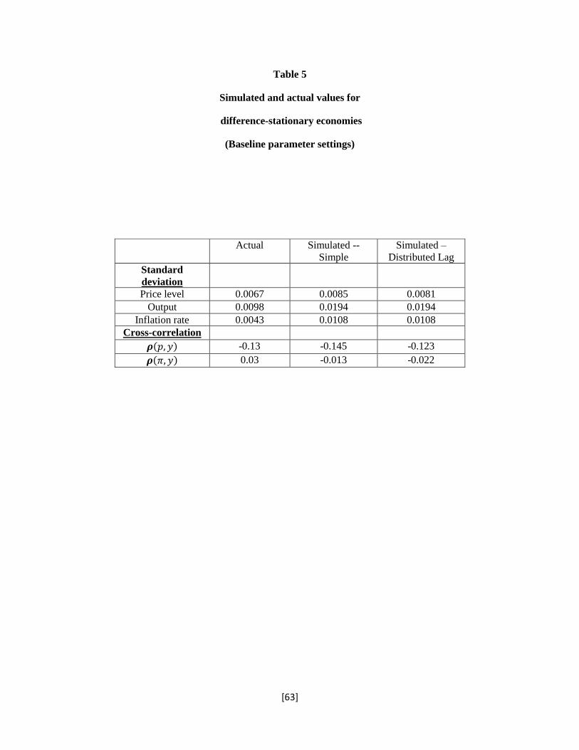
[63]

Table 5

Simulated and actual values for

difference-stationary economies

(Baseline parameter settings)

Actual Simulated --

Simple

Simulated –

Distributed Lag

Standard

deviation

Price level 0.0067 0.0085 0.0081

Output 0.0098 0.0194 0.0194

Inflation rate 0.0043 0.0108 0.0108

Cross-correlation

( ) -0.13 -0.145 -0.123

( ) 0.03 -0.013 -0.022

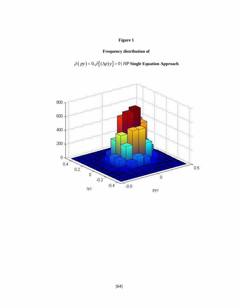
[64]

Figure 1

Frequency distribution of

ˆ ˆ0, ( ) 0 |py p y HP Single Equation Approach

[65]

Figure 2

Frequency distribution of

ˆ ˆ0, ( ) 0 |py p y DS : Single Equation Approach

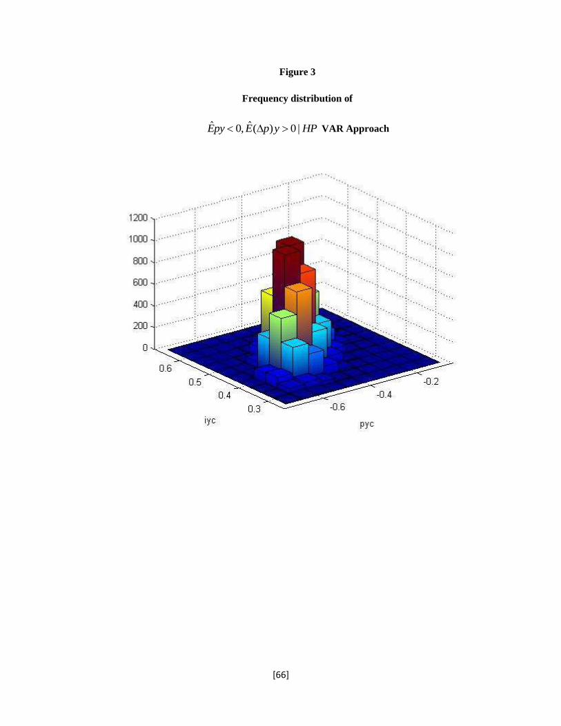
[66]

Figure 3

Frequency distribution of

ˆ ˆ0, ( ) 0 |Epy E p y HP VAR Approach

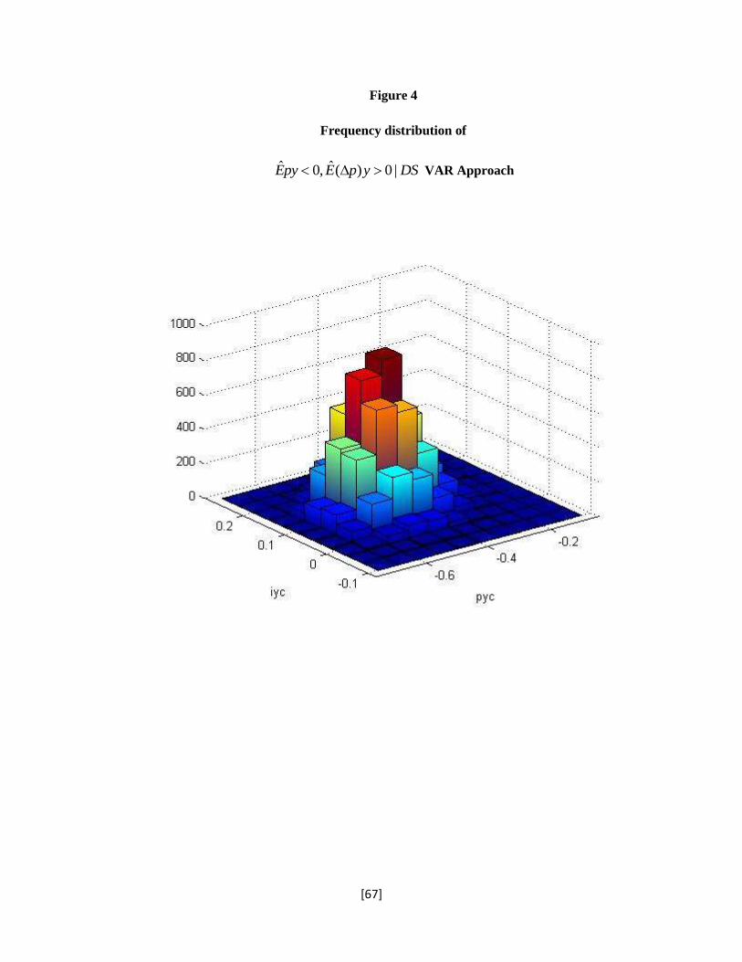
[67]

Figure 4

Frequency distribution of

ˆ ˆ0, ( ) 0 |Epy E p y DS VAR Approach