The Cyclical Behaviorof the Price-Cost Markup

Christopher J. NekardaFederal Reserve Board of Governors

Valerie A. RameyUniversity of California, San Diego

and NBER

First version: July 2009This version: June 2010

Abstract

Countercyclical markups constitute the key transmission mechanism for monetaryand other “demand” shocks in textbook New Keynesian models. This paper teststhe foundation of those models by studying the cyclical properties of the markupof price over marginal cost. The first part of the paper studies markups in the ag-gregate economy and the manufacturing sector. We use Bils’s (1987) insights forconverting average cost to marginal cost, but do so with richer data. We find thatall measures of markups are either procyclical or acyclical. Moreover, we showthat monetary shocks lead markups to fall with output. The last part of the papermerges input-output information on shipments to the government with detailedindustry data to study the effect of demand changes on industry-level markups.Industry-level markups are found to be acyclical in response to demand changes.

JEL codes: E32, L16, J31Keywords: markup, cyclicality

The views in this paper are those of the authors and do not necessarily represent the views or policies ofthe Board of Governors of the Federal Reserve System or its staff. We are grateful to Mark Bils, OlivierCoibion, Steve Davis, Davide Debortoli, David Lebow, Robert Hall, Garey Ramey, Harald Uhlig, RafWouters and participants at numerous seminars for helpful comments. Ben Backes provided excellentresearch assistance. Valerie Ramey gratefully acknowledges financial support from National ScienceFoundation grant SES-0617219 through the National Bureau of Economic Research.

How markups move, in response to what, and why, is however nearly terraincognita for macro. . . . [W]e are a long way from having either a clearpicture or convincing theories, and this is clearly an area where research isurgently needed.

— Blanchard (2008), p. 18.

1 Introduction

The markup of price over marginal cost plays a key role in a number of macroeco-

nomic models. For example, in Rotemberg and Woodford’s (1992) model, an increase

in government spending leads to increases in both hours and real wages because imper-

fect competition generates a countercyclical markup. In the textbook New Keynesian

model, sticky prices combined with procyclical marginal cost imply that an expansion-

ary monetary shock or government spending shock lowers the average markup (Good-

friend and King, 1997). This result also holds in the leading New Keynesian models

with both sticky prices and sticky wages, such as Erceg et al. (2000); Smets and Wouters

(2003, 2007); Christiano et al. (2005). In Jaimovich and Floetotto’s (2008) model,

procyclical entry of firms leads to countercyclical markups, and hence to procyclical

movements in measured productivity.

The dependence of Keynesian models on countercyclical markups is a feature only

of the models formulated since the early 1980s. From the 1930s through the 1970s,

the Keynesian model was founded on the assumption of sticky wages (e.g. Keynes

(1936), Phelps (1968), Taylor (1980). Some researchers believed that the implica-

tions of this model were at odds with the cyclical properties of real wages, leading

to a debate known as the “Dunlop-Tarshis” controversy.1 In response to the perceived

disparity between the data and predictions of the traditional Keynesian model, the lit-

erature shifted in the early 1980s to the assumption of sticky prices rather than sticky

wages (e.g. Gordon (1981), Rotemberg (1982)). This type of model emerged as the

leading textbook New Keynesian model. Virtually all current New Keynesian models

incorporate the notion that markups fall in response to positive demand shifts.

Estimating the cyclicality of markups is one of the more challenging measurement

1. In fact, Dunlop (1938) and Tarshis (1939) were repeatedly misquoted by the literature as showingthat real wages were procyclical. Neither of them showed this. Both authors showed that money wagesand real wages were positively correlated, and Tarshis went on to show that real wages were in factnegatively correlated with aggregate employment.

1

issues in macroeconomics. Theory directs comparing price and marginal cost; how-

ever, available data typically include only average cost. Papers studying the cyclicality

of marginal cost and markups either accept average cost as is (e.g., Domowitz et al.,

1986; Chirinko and Fazzari, 1994) or make assumptions on how marginal cost is re-

lated to average cost (e.g., Bils, 1987; Rotemberg and Woodford, 1991, 1999; Galí

et al., 2007). Using measures of price-average cost margins, Domowitz et al. (1986)

find that markups are positively correlated with the growth of industry demand, sug-

gesting that markups are procyclical. Bils (1987) estimates marginal cost in manufac-

turing under several assumptions about overtime and adjustment costs and concludes

that markups there are countercyclical. Chirinko and Fazzari (1994) apply a dynamic

factor model to estimate markups, and find that they are procyclical in nine of the

eleven 4-digit industries they analyze. Rotemberg and Woodford (1991, 1999) study

the economy more broadly and present several mitigating reasons why seemingly pro-

cyclical patterns in measures of the average markup should be discounted.

In this paper, we present evidence that most measures of the markup are procycli-

cal or acyclical. Moreover, they increase in response to positive monetary shocks and

are unresponsive to government spending shocks. The first part of the paper presents

the evidence using aggregate data. Markups based on average wages are procyclical,

hitting troughs during recessions and reaching peaks in the middle of expansions. Be-

cause of concerns that average wages do not adequately capture marginal costs, we use

insights from Bils (1987) to make adjustments to convert average wages into marginal

costs. In contrast to Bils, we find that all measures of the markup remain procyclical

or acyclical even after adjustment. We trace the main source of the difference to Bils’s

use of annual data, since replication of his methods on quarterly data yield procyclical

or acyclical markups. We also consider generalizations of the standard Cobb-Douglas

production function and find little effect. We then consider the response of our various

markup measures to monetary policy shocks. We find that a contractionary monetary

policy shock leads to a fall in both output and the markup. This result raises questions

about the basic propagation mechanism of the current versions of the New Keynesian

model: If the markup does not move countercyclically, how can money have short-run

real effects?

In the last part of the paper we analyze the markup in a panel of industries. We

match detailed input-output (IO) data on government demand and its downstream

linkages with data on employment, hours, and output. We argue that the government

2

demand variable we construct is an excellent instrument for determining the effects of

shifts in demand on markups. We find that an increase in output associated with higher

government spending has essentially no effect on markups at an annual frequency.

2 Theoretical Framework

In this section we review the theory that guides our empirical investigation. We first

derive the marginal cost of increasing output by raising average hours per worker. We

then derive an expression for converting data on average wages to marginal wages.

Finally, we consider a more general production function.

The theoretical markup, M, is defined as

(1) M=P

MC,

where P is the price of output and MC is the nominal marginal cost of increasing

output. The inverse of the right hand side of equation 1, MC/P, is also known as the

real marginal cost.

As Basu and Fernald (1997a) point out, a cost-minimizing firm should equalize the

marginal cost of increasing output across all possible margins for varying production.

Thus, it is valid to consider the marginal cost of varying output by changing a partic-

ular input. As in Bils (1987) and Rotemberg and Woodford (1999), we focus on the

labor input margin, and in particular on hours per worker. We assume that there are

potential costs of adjusting the number of employees and the capital stock, but no costs

of adjusting hours per worker.2

Focusing on the static aspect of this cost-minimization problem, consider the prob-

lem of a firm that chooses hours per worker, h, to minimize

(2) Cost=WAhN + other terms not involving h,

subject to Y = F(AhN , . . .). WA is the average hourly wage, N is the number of workers,

Y is output, and A is the level of labor-augmenting technology. Bils (1987) argues that

the average wage paid by a firm may be increasing in the average hours per worker

2. Hamermesh and Pfann’s (1996) summary of the literature suggests that adjustment costs on thenumber of employees are relatively small and that adjustment costs on hours per worker are essentiallyzero.

3

because of the additional cost of overtime hours. We capture this assumption by speci-

fying the average wage as:

(3) WA =WS

�

1+ρθv

h

�

.

where WS is the straight-time wage, ρ is the premium for overtime hours, θ is the

fraction of overtime hours that command a premium, and v/h is the ratio of average

overtime hours to total hours. The term ρθ v/h captures the idea that firms may have

to pay a premium for hours worked beyond the standard workweek.3 Bils did not

include the θ term in his specification because he used manufacturing data from the

Current Employment Statistics (CES), in which overtime hours are defined as those

hours commanding a premium, where θ = 1. In several of our data sources, we define

overtime hours as those hours in excess of 40 hours per week. Because overtime pre-

mium regulations do not apply to all workers, we must allow for the possibility that θ

is less than unity and my vary over time.

We assume that the firm takes the straight-time wage, the overtime premium, and

the fraction of workers receiving premium pay as given, but recognizes the potential

effect of raising h on overtime hours v. Letting λ be the Lagrange multiplier on the

constraint, we obtain the first-order condition for h as:

(4) WS

�

1+ρθ�

dv

dh

��

= λF1(AhN , . . .)A,

where dv/dh is the amount by which average overtime hours rise for a given increase

in average total hours and F1 is the derivative of the production function with respect

to effective labor, AhN . The multiplier λ is equal to marginal cost, so the marginal cost

of increasing output by raising hours per worker is given by:

(5) MC = λ=WS

�

1+ρθ�

dvdh

��

AF1(AhN , . . .).

The denominator of equation 5 is the marginal product of increasing hours per worker;

the numerator is the marginal cost of increasing average hours per worker. As discussed

above, this marginal cost should also be equal to the marginal cost of raising output by

3. It would also be possible to distinguish wages paid for part-time work versus full-time work.However, Hirsch (2005) finds that nearly all of the difference in hourly wages between part-time andfull-time workers can be attributed to worker heterogeneity rather than to a premium for full-time work.

4

increasing employment or the capital stock. If there are adjustment costs involved in

changing those factors, the marginal cost would include an adjustment cost component.

Focusing on the hours margin obviates the need to estimate adjustment costs.

Equation 5 makes it clear that the marginal cost of increasing hours per worker is

not equal to the average wage, as is commonly assumed. Following Bils (1987), we

call the term in the numerator the “marginal wage” and denote it by WM:

(6) WM =WS

�

1+ρθ�

dv

dh

��

.

To the extent that the marginal wage has different cyclical properties from the average

wage, markup measures that use the average wage may embed cyclical biases. Bils

(1987) used approximations to the marginal wage itself to substitute for marginal cost

in his markup measure. We instead use an adjustment that does not require approxima-

tion. In particular, we combine the expressions for the average wage and the marginal

wage to obtain their ratio:

(7)WM

WA=

1+ρθ�

dvdh

�

1+ρθ�

vh

� .

This ratio can be used to convert the observed average wage to the theoretically-correct

marginal wage required to estimate the markup. We show in section 3 that the ratio

of overtime hours to average hours, v/h, is procyclical, and that θ is roughly constant.

Thus, the denominator in equation 7 is procyclical. How WM/WA evolves over the busi-

ness cycle depends on the relative cyclicality of dv/dh. The fact that v/h increases

with h does not imply that dv/dh increases with h. It can be shown that for a con-

stant θ , d2v/dh2 > 0 is a necessary, but not sufficient, condition for the wage ratio

to be increasing in h. Thus, it is possible for v/h to be procyclical, but WM/WA to be

countercyclical.

A second complication with estimating the markup is estimating the marginal prod-

uct of labor. If the production function is Cobb-Douglas, then the marginal product of

labor is proportional to the average product. Consider a more general case in which

the production function has constant elasticity of substitution (CES):

(8) Y =h

α (AhN)σ−1σ + (1−α)K

σ−1σ

iσσ−1

,

5

where σ is the elasticity of substitution between capital and labor. The derivative with

respect to effective labor (the F1 needed for equation 5) is

(9)∂ Y

∂ (AhN)= α

�

Y

AhN

�1σ

.

The exponent in equation 9 is the reciprocal of the elasticity of substitution. If the

elasticity of substitution is unity, this specializes to the Cobb-Douglas case. On the

other hand, if the elasticity of substitution is less than unity, then the exponent will be

greater than unity.

In the simple case where the marginal wage is equal to the average wage and

the marginal product of labor is proportional to the average product (as in the Cobb-

Douglas case), then the markup is given by

(10) MCDA =

P

WA/ [α (Y/hN)]=α

s,

where α is the exponent on labor input in the production function and s is the labor

share. In the case where the wage is increasing in average hours, the markup can be

written as

(11) MCDM =

P

WM/ [α (Y/hN)]=

α

s�

WM/WA

� ,

where we use equation 7 to convert average wages to marginal wages. Finally, allowing

for a CES production function, we obtain the markup

MCESM =

P

WM/h

Aα (Y/AhN)1σ

i(12)

=α

s�

WM/WA

�

�

Y

AhN

�1σ−1

.

One important issue is that Y should be gross output. As Basu and Fernald (1997b)

argue, “value added is not a natural measure of output and can in general be inter-

preted as such only with perfect competition.”4 Because any nonconstant, nonunity

markup requires imperfect competition, markup measures should be based on gross

4. Basu and Fernald (1997b), p. 251.

6

output, not value added. Unfortunately, no measures of gross output are available for

the broad aggregates studied in section 4 so we must use value added. We use gross

output when studying the markup at the industry level in section 7.

3 Estimating the Marginal-Average Wage Adjustment

This section describes the estimation of the four components of the marginal-average

wage adjustment factor. For expositional purposes, we repeat equation 7:

[7]WM

WA=

1+ρθ�

dvdh

�

1+ρθ�

vh

� .

To construct the ratio of marginal to average wages, we require (1) estimates of the

ratio of overtime hours to average hours, v/h; (2) estimates of the marginal change in

overtime hours with respect to a change in average total hours, dv/dh; (3) the fraction

of overtime hours that command a premium, θ ; and (4) the premium for overtime

hours, ρ.

3.1 Measuring v/h

Most researchers analyzing the cyclical behavior of overtime hours have focused on

production workers in manufacturing, since this group is the only one for whom data

on overtime hours are readily available. The manufacturing sector is not representative

of the entire U.S. economy, however. Even at its post-World War II peak, manufacturing

accounted for only 25 percent of employment; it now accounts for only 9 percent of

employment. Thus, it is important to look at broader measures of the economy.

To this end, we use three main data sources. First, we exploit an overlooked data

source in order to construct a time series on the distribution of hours worked in the en-

tire civilian economy. The Bureau of Labor Statistics (BLS)’s Employment and Earnings

publication provides information on persons at work by hours of work, total persons

at work, and average hours worked by persons at work, derived from the Current Pop-

ulation Survey (CPS). These data are available monthly beginning in May 1960. The

number of persons at work are available only within particular ranges of hours worked,

such as 35–39 hours per week, 40 hours per week, 41–48 hours per week, etc. To ap-

proximate the distribution of hours worked, we use data from the CPS to calculate a

7

time-varying average of actual hours worked for each published range. We seasonally

adjust the monthly data. The appendix contains a complete list of data sources and

additional details of our methodology. Second, we use CES data for manufacturing.

The CES provides monthly data on average weekly hours and average weekly over-

time hours of production and nonsupervisory workers in manufacturing going back to

1956. This is an establishment-based survey. Third, we use monthly CPS data, which

are available from 1976 to 2007. This data source allows us to measure hours for all

workers in manufacturing, not just production workers.

A key different between the CES data and the two CPS data sources is the defini-

tion of overtime hours. The CES defines overtime hours as any hours that are paid a

premium. The CPS makes no distinction between overtime premium hours and other

hours. Thus, we define overtime hours in the CPS data as any hours worked above 40

hours per week, including those possibly worked on a second job. The fact that not all

of these hours are paid a premium will be discussed below when we estimate θ .

Figure 1 shows hours series for all workers in the aggregate economy, based on

CPS data. The top panel plots average weekly hours per worker, the middle panel

plots average weekly hours in excess of 40 (“overtime hours”), and the bottom panel

plots the percent of total hours worked that are overtime hours. The bottom panel

shows the estimates from Employment and Earnings (labeled “aggregate”) as well as

our estimates based on individual data from the monthly CPS (available from 1976

to 2007). All three series show pronounced low-frequency movements, decreasing

throughout the 1960s and 1970s and rising over the 1980s and 1990s. They also

appear to be mildly procyclical, although the low-frequency movements dominate.

Figure 2 shows the CES-based hours series for production and nonsupervisory work-

ers in manufacturing (labeled “aggregate”), as well as the CPS-based ratio of overtime

hours to average hours for all manufacturing workers in the bottom graph. All se-

ries display noticeable procyclicality, as well as important low frequency movements.

The procyclical fraction of overtime hours in the bottom panel implies that average

overtime hours varies more than average hours. The bottom panel also shows that

despite the difference in the worker universe (establishment-level production workers

versus household survey total workers) and the different definitions of overtime hours,

the two ratios move together fairly closely, particular during the first ten years of the

overlap. The correlation for the entire overlap period is 0.95. The results are almost

indistinguishable when we substitute one for the other in our wage factor. Thus, when

8

we examine wage factors for the entire period, we will use the CES ratio of overtime

hours to average hours. 5

The series shown in the bottom panels of figures 1 and 2 are the first element

needed to estimate the marginal-average wage adjustment factor. How overtime hours

vary with changes in average hours is an important determinant of the cyclicality of

marginal cost.

3.2 Estimating dv/dh

The second key element in the wage factor is the marginal change in overtime hours.

Bils (1987) speculated that a given increase in average hours would require more over-

time hours if the starting level of average hours was higher. He used CES data from

manufacturing to calculate the change in average overtime hours, ∆vt , and the change

in average hours, ∆ht , and related them with the following difference approximation:

∆vt = α+ηt∆ht + ξt .

To capture the possible dependence of dv/dh on the level of hours, he specified ηt as a

cubic function of lagged average hours and time trends.6

Averages hours based on aggregate data are not ideal for measuring this component

for several reasons. First, as Bils pointed out, higher moments of the average hours

distribution could also matter because all workers do not work the same amount of

hours. Second, in the aggregate data it is not unusual for dh = 0 but dv 6= 0, which

is problematic for both the interpretation and the econometric estimation. Ideally, we

want to construct the ratio of the change in overtime hours to the change in average

hours by individual workers and then take the economy-wide average. That is, we

want to construct the “average marginal” change in overtime hours with respect to a

change in average hours. The ideal way to do this is to use panel data on individual

5. One would expect the production worker series to be even closer to the total series in the early partof the sample. In 1956, production workers accounted for over 80 percent of workers in manufacturing;in 1976, they were 75 percent; and by 2009 they were 70 percent.

6. Mazumder (2010) instead regresses the level of vt on a polynomial in ht and then takes thederivative. The problem with this procedure is that low frequency movements (evident in figure 2)rather than business cycle fluctuations determine the coefficient estimates. Our comparison of the twomethods suggests that Mazumder’s (2010) method produces estimates of the effects of average hourson dv/dh that are three times larger than those produced by Bils’s first-difference method.

9

workers.7

To construct this series, we use Nekarda’s (2009) Londitudinal Population Database,

a monthly panel data set constructed from the CPS microdata that matches individu-

als across all months in the survey. The data are available from 1976 to 2007. For

each matched individual who was employed two consecutive months, we compute the

change in average hours ∆hi t and the change in overtime hours ∆vi t , where overtime

hours are any hours worked above 40, including those hours from secondary jobs. By

studying only those employed two consecutive months, we isolate the intensive mar-

gin, as required by the theory.8 We construct the ratio dvi t/dhi t for each individual

and compute the average of this ratio for all individuals each month. We do this for all

civilian workers as well as for all workers in manufacturing. The Appendix discusses

the details of our method.

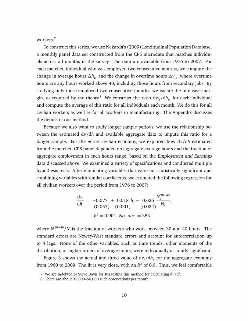
Because we also want to study longer sample periods, we use the relationship be-

tween the estimated dv/dh and available aggregate data to impute this ratio for a

longer sample. For the entire civilian economy, we explored how dv/dh estimated

from the matched CPS panel depended on aggregate average hours and the fraction of

aggregate employment in each hours range, based on the Employment and Earnings

data discussed above. We examined a variety of specifications and conducted multiple

hypothesis tests. After eliminating variables that were not statistically significant and

combining variables with similar coefficients, we estimated the following regression for

all civilian workers over the period from 1976 to 2007:

dvt

dht= −0.077(0.057)

+ 0.018(0.001)

ht − 0.626(0.024)

N 30−40t

Nt,

R2 = 0.901, No. obs. = 383

where N 30−40/N is the fraction of workers who work between 30 and 40 hours. The

standard errors are Newey-West standard errors and account for autocorrelation up

to 4 lags. None of the other variables, such as time trends, other moments of the

distribution, or higher orders of average hours, were individually or jointly significant.

Figure 3 shows the actual and fitted value of dvt/dht for the aggregate economy

from 1960 to 2009. The fit is very close, with an R2 of 0.9. Thus, we feel comfortable

7. We are indebted to Steve Davis for suggesting this method for calculating dv/dh.8. There are about 35,000–50,000 such observations per month.

10

using the fitted values for the entire sample.

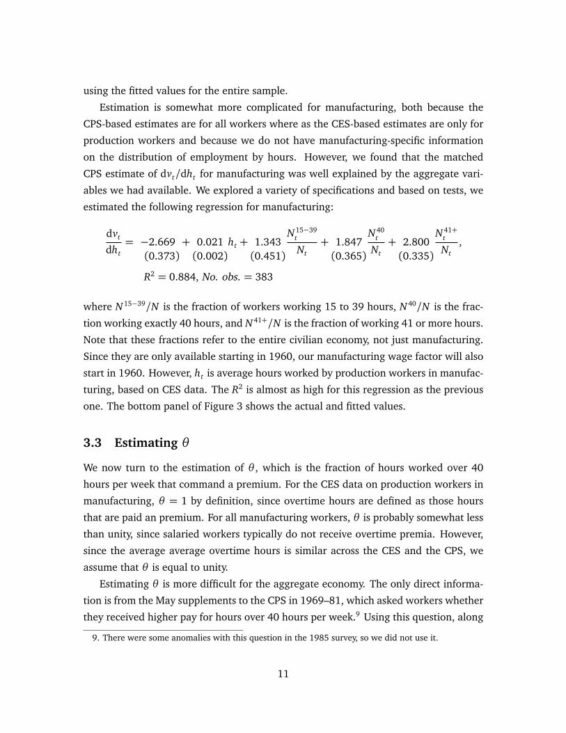
Estimation is somewhat more complicated for manufacturing, both because the

CPS-based estimates are for all workers where as the CES-based estimates are only for

production workers and because we do not have manufacturing-specific information

on the distribution of employment by hours. However, we found that the matched

CPS estimate of dvt/dht for manufacturing was well explained by the aggregate vari-

ables we had available. We explored a variety of specifications and based on tests, we

estimated the following regression for manufacturing:

dvt

dht= −2.669(0.373)

+ 0.021(0.002)

ht + 1.343(0.451)

N 15−39t

Nt+ 1.847(0.365)

N 40t

Nt+ 2.800(0.335)

N 41+t

Nt,

R2 = 0.884, No. obs. = 383

where N 15−39/N is the fraction of workers working 15 to 39 hours, N 40/N is the frac-

tion working exactly 40 hours, and N 41+/N is the fraction of working 41 or more hours.

Note that these fractions refer to the entire civilian economy, not just manufacturing.

Since they are only available starting in 1960, our manufacturing wage factor will also

start in 1960. However, ht is average hours worked by production workers in manufac-

turing, based on CES data. The R2 is almost as high for this regression as the previous

one. The bottom panel of Figure 3 shows the actual and fitted values.

3.3 Estimating θ

We now turn to the estimation of θ , which is the fraction of hours worked over 40

hours per week that command a premium. For the CES data on production workers in

manufacturing, θ = 1 by definition, since overtime hours are defined as those hours

that are paid an premium. For all manufacturing workers, θ is probably somewhat less

than unity, since salaried workers typically do not receive overtime premia. However,

since the average average overtime hours is similar across the CES and the CPS, we

assume that θ is equal to unity.

Estimating θ is more difficult for the aggregate economy. The only direct informa-

tion is from the May supplements to the CPS in 1969–81, which asked workers whether

they received higher pay for hours over 40 hours per week.9 Using this question, along

9. There were some anomalies with this question in the 1985 survey, so we did not use it.

11

with information on hours worked, we construct a measure of the percent of hours

worked over 40 that are paid an overtime premium.10

Unfortunately, the key question on premium pay was dropped from the May supple-

ment after 1985. A potential alternative source of information is the BLS’s Employee

Costs for Employee Compensation (ECEC) survey which provides information on total

compensation, straight time wages and salaries, and various benefits, such as overtime

pay, annually from 1991 to 2001 and quarterly from 2002 to the present. If one as-

sumes a particular statutory overtime premium, then one can construct an estimate of

θ from these data. We assume that the statutory premium is 50 percent and construct

a θ accordingly.

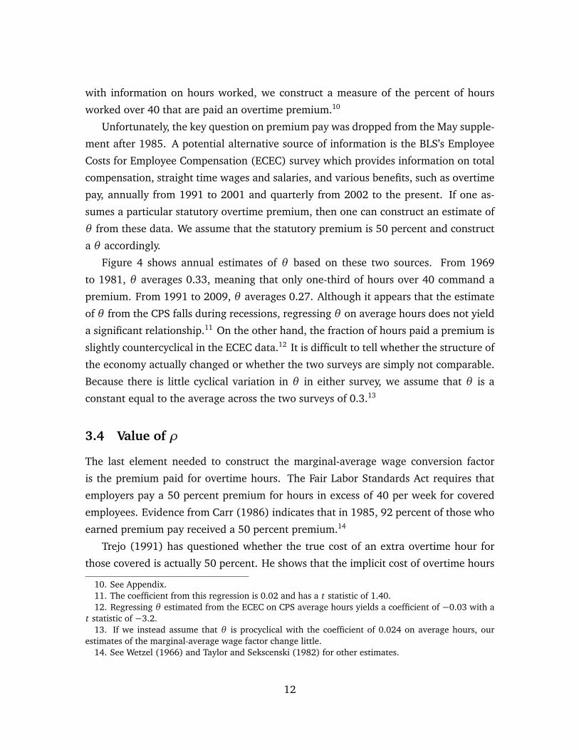
Figure 4 shows annual estimates of θ based on these two sources. From 1969

to 1981, θ averages 0.33, meaning that only one-third of hours over 40 command a

premium. From 1991 to 2009, θ averages 0.27. Although it appears that the estimate

of θ from the CPS falls during recessions, regressing θ on average hours does not yield

a significant relationship.11 On the other hand, the fraction of hours paid a premium is

slightly countercyclical in the ECEC data.12 It is difficult to tell whether the structure of

the economy actually changed or whether the two surveys are simply not comparable.

Because there is little cyclical variation in θ in either survey, we assume that θ is a

constant equal to the average across the two surveys of 0.3.13

3.4 Value of ρ

The last element needed to construct the marginal-average wage conversion factor

is the premium paid for overtime hours. The Fair Labor Standards Act requires that

employers pay a 50 percent premium for hours in excess of 40 per week for covered

employees. Evidence from Carr (1986) indicates that in 1985, 92 percent of those who

earned premium pay received a 50 percent premium.14

Trejo (1991) has questioned whether the true cost of an extra overtime hour for

those covered is actually 50 percent. He shows that the implicit cost of overtime hours

10. See Appendix.11. The coefficient from this regression is 0.02 and has a t statistic of 1.40.12. Regressing θ estimated from the ECEC on CPS average hours yields a coefficient of −0.03 with a

t statistic of −3.2.13. If we instead assume that θ is procyclical with the coefficient of 0.024 on average hours, our

estimates of the marginal-average wage factor change little.14. See Wetzel (1966) and Taylor and Sekscenski (1982) for other estimates.

12

is lower than 50 percent because straight-time wages are lower in industries that offer

more overtime. Hamermesh (2006) updates his analysis and finds supporting results:

the implicit overtime premium is 25 percent, not 50 percent. The following theory is

consistent with these results. Workers and firms bargain over a job package that in-

volves hours and total compensation. If workers’ marginal disutility of overtime hours

is less than the statutory premium for overtime hours, then workers and firms in indus-

tries with higher average overtime hours will adjust to overtime regulations by agreeing

to a lower straight-time wage. This implicit contract means that when the firm pays the

worker a 50 percent premium for an overtime hour, part of that premium compensates

the worker for the true marginal disutility of overtime, but part is simply a payment on

a debt incurred to the worker because the contracted straight-time wage is lower.

In light of these results, we construct our markups under two alternative assump-

tions. First, we assume that the effective marginal overtime premium is equal to the

statutory premium, so that the ρ in both the numerator and denominator of equation 7

are equal to 0.50. Second, we assume that the effective marginal overtime premium is

equal to Hamermesh’s (2006) estimate of 0.25. This means that the ρ in the numerator

of equation 7 is equal to 0.25; however, since the average wage data includes the 50

percent statutory premium, the ρ in the denominator remains at 0.50.

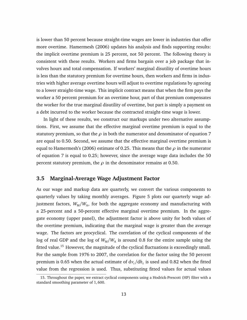
3.5 Marginal-Average Wage Adjustment Factor

As our wage and markup data are quarterly, we convert the various components to

quarterly values by taking monthly averages. Figure 5 plots our quarterly wage ad-

justment factors, WM/WA, for both the aggregate economy and manufacturing with

a 25-percent and a 50-percent effective marginal overtime premium. In the aggre-

gate economy (upper panel), the adjustment factor is above unity for both values of

the overtime premium, indicating that the marginal wage is greater than the average

wage. The factors are procyclical. The correlation of the cyclical components of the

log of real GDP and the log of WM/WA is around 0.8 for the entire sample using the

fitted value.15 However, the magnitude of the cyclical fluctuations is exceedingly small.

For the sample from 1976 to 2007, the correlation for the factor using the 50 percent

premium is 0.65 when the actual estimate of dvt/dht is used and 0.82 when the fitted

value from the regression is used. Thus, substituting fitted values for actual values

15. Throughout the paper, we extract cyclical components using a Hodrick-Prescott (HP) filter with astandard smoothing parameter of 1,600.

13

tends to bias the wage factor in the procyclical direction, which will bias the markup in

the countercyclical direction; however, it will make little difference because the mag-

nitude of the fluctuations is so small. The correlations using the 25 percent premium

are slightly lower.

In manufacturing (lower panel) the adjustment factor is also procyclical. The cor-

relation of the cyclical component of the adjustment factor in manufacturing with real

GDP is 0.34 for the 25 percent premium and 0.25 for the 50 percent premium for

the sample from 1960 to 2009, using the various fitted values. For the sample 1976

to 2007, the correlations are between 0.44 and 0.57 when the true values are used

and between 0.51 and 0.81 when the fitted values are used. Again, the use of fitted

values tends to make the ratio of marginal wage to average wage more procyclical as

compared to when the actual estimates are used.

4 The Cyclical Behavior of Markups

As discussed in section 2, the average markup is proportional to the inverse of the labor

share. We study four measures of the labor share covering several broad aggregates.

Our first measure is the BLS’s index of labor share for the private business sector. This

is the broadest aggregate measure and it covers all compensation in this sector. We

also consider two labor share measures constructed from the U.S. national income and

product accounts (NIPA) that include only wage and salaries and exclude fringe bene-

fits. Labor shares for private business and manufacturing are constructed by dividing

wage and salary disbursements by total income. Finally, we consider a measure for the

nonfinancial corporate business sector that divides labor compensation by gross value

added less indirect taxes.16 The Appendix provides additional details.

4.1 The Markup Measured with Average Wages

Figure 6 displays measures of the markup based on average wages, as defined in equa-

tion 10 (i.e., assuming Cobb-Douglas production). The top series is the markup in non-

financial corporate business, the measure favored by Rotemberg and Woodford (1999).

The middle two series plot the markup in private business using NIPA and BLS data.

16. The first three measures do not subtract indirect taxes because of data availability. However,in nonfinancial corporate business we find that the tax-adjusted markup is more procyclical than theunadjusted markup. Thus, the measures that do not adjust for indirect taxes have a countercyclical bias.

14

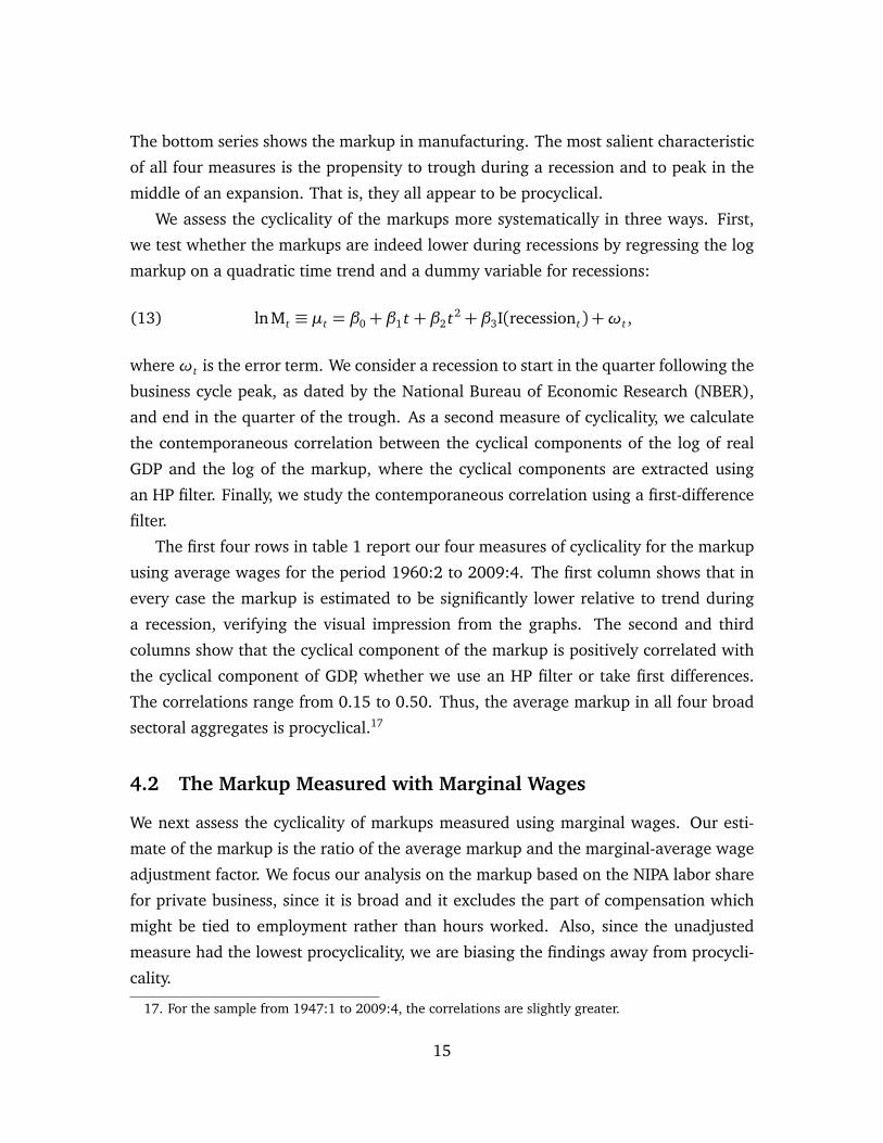
The bottom series shows the markup in manufacturing. The most salient characteristic

of all four measures is the propensity to trough during a recession and to peak in the

middle of an expansion. That is, they all appear to be procyclical.

We assess the cyclicality of the markups more systematically in three ways. First,

we test whether the markups are indeed lower during recessions by regressing the log

markup on a quadratic time trend and a dummy variable for recessions:

(13) lnMt ≡ µt = β0+ β1 t + β2 t2+ β3I(recessiont) +ωt ,

whereωt is the error term. We consider a recession to start in the quarter following the

business cycle peak, as dated by the National Bureau of Economic Research (NBER),

and end in the quarter of the trough. As a second measure of cyclicality, we calculate

the contemporaneous correlation between the cyclical components of the log of real

GDP and the log of the markup, where the cyclical components are extracted using

an HP filter. Finally, we study the contemporaneous correlation using a first-difference

filter.

The first four rows in table 1 report our four measures of cyclicality for the markup

using average wages for the period 1960:2 to 2009:4. The first column shows that in

every case the markup is estimated to be significantly lower relative to trend during

a recession, verifying the visual impression from the graphs. The second and third

columns show that the cyclical component of the markup is positively correlated with

the cyclical component of GDP, whether we use an HP filter or take first differences.

The correlations range from 0.15 to 0.50. Thus, the average markup in all four broad

sectoral aggregates is procyclical.17

4.2 The Markup Measured with Marginal Wages

We next assess the cyclicality of markups measured using marginal wages. Our esti-

mate of the markup is the ratio of the average markup and the marginal-average wage

adjustment factor. We focus our analysis on the markup based on the NIPA labor share

for private business, since it is broad and it excludes the part of compensation which

might be tied to employment rather than hours worked. Also, since the unadjusted

measure had the lowest procyclicality, we are biasing the findings away from procycli-

cality.

17. For the sample from 1947:1 to 2009:4, the correlations are slightly greater.

15

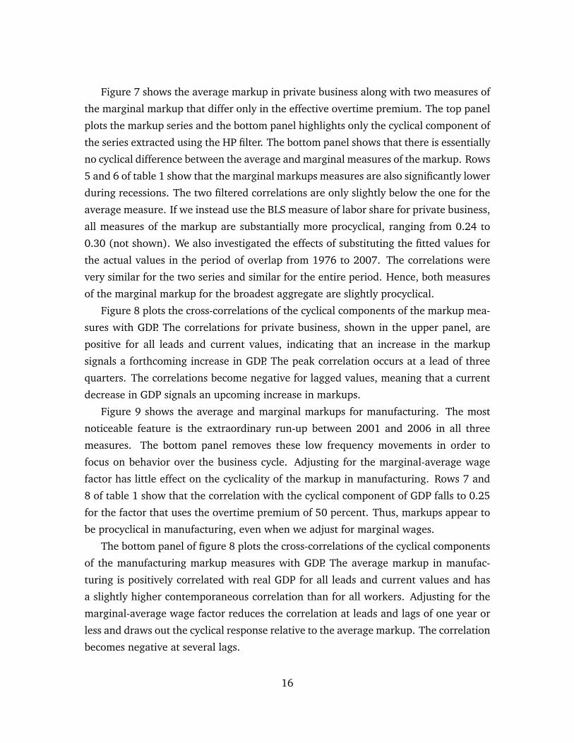
Figure 7 shows the average markup in private business along with two measures of

the marginal markup that differ only in the effective overtime premium. The top panel

plots the markup series and the bottom panel highlights only the cyclical component of

the series extracted using the HP filter. The bottom panel shows that there is essentially

no cyclical difference between the average and marginal measures of the markup. Rows

5 and 6 of table 1 show that the marginal markups measures are also significantly lower

during recessions. The two filtered correlations are only slightly below the one for the

average measure. If we instead use the BLS measure of labor share for private business,

all measures of the markup are substantially more procyclical, ranging from 0.24 to

0.30 (not shown). We also investigated the effects of substituting the fitted values for

the actual values in the period of overlap from 1976 to 2007. The correlations were

very similar for the two series and similar for the entire period. Hence, both measures

of the marginal markup for the broadest aggregate are slightly procyclical.

Figure 8 plots the cross-correlations of the cyclical components of the markup mea-

sures with GDP. The correlations for private business, shown in the upper panel, are

positive for all leads and current values, indicating that an increase in the markup

signals a forthcoming increase in GDP. The peak correlation occurs at a lead of three

quarters. The correlations become negative for lagged values, meaning that a current

decrease in GDP signals an upcoming increase in markups.

Figure 9 shows the average and marginal markups for manufacturing. The most

noticeable feature is the extraordinary run-up between 2001 and 2006 in all three

measures. The bottom panel removes these low frequency movements in order to

focus on behavior over the business cycle. Adjusting for the marginal-average wage

factor has little effect on the cyclicality of the markup in manufacturing. Rows 7 and

8 of table 1 show that the correlation with the cyclical component of GDP falls to 0.25

for the factor that uses the overtime premium of 50 percent. Thus, markups appear to

be procyclical in manufacturing, even when we adjust for marginal wages.

The bottom panel of figure 8 plots the cross-correlations of the cyclical components

of the manufacturing markup measures with GDP. The average markup in manufac-

turing is positively correlated with real GDP for all leads and current values and has

a slightly higher contemporaneous correlation than for all workers. Adjusting for the

marginal-average wage factor reduces the correlation at leads and lags of one year or

less and draws out the cyclical response relative to the average markup. The correlation

becomes negative at several lags.

16

4.3 CES Production Function

We also consider a measure of the aggregate markup under the assumption that the

production function has a lower elasticity of substitution between capital and labor

than the Cobb-Douglas production function. This markup is based on the expression

in equation 12. The extra term in this markup measure consists of output divided by

the product of total hours and the level of technology (Y /AhN) raised to the inverse

of the elasticity of substitution. Thus, this measure requires an estimate of the level of

technology (A), as well as the elasticity of substitution.

We consider two methods of estimating A. The first estimates technology as the HP

trend in labor productivity. This method assumes that all business cycle variation in la-

bor productivity is due to factors other than technology. The second uses Galí’s (1999)

structural vector autoregression (VAR) method for identifying a technology shock as

the only shock that has a permanent effect on labor productivity. To do this, we es-

timate a bivariate VAR with productivity growth and the growth of hours per capita

using quarterly data for 1948–2008. We define technology as the part of labor produc-

tivity explained by the technology shock. The estimates from this method imply that

much of the cyclical variation in labor productivity is due to technology.

Chirinko (2008) surveys the literature estimating the elasticity of substitution be-

tween capital and labor and concludes that the elasticity is in the range of 0.4 to 0.6.

Thus, we use an elasticity of substitution between capital and labor of 0.5, along with

the marginal wage factor with an overtime premium of 25 percent. Rows 9 and 10 of

table 1 report the cyclicality of this markup with the two different estimates of tech-

nology. The first column shows that both measures are significantly lower during a

recession. The third column shows that both measures are even more procyclical than

the one that assumes Cobb-Douglas; the correlation with the cyclical component of

GDP is around 0.3.18

To summarize our results, we find that markups measured using average wages are

procyclical in the aggregate economy and in manufacturing. Adjusting the markup for

the difference between marginal and average wage yields only slight procyclicality for

our main measure. The procyclicality of the markup in manufacturing remains even

after adjustment.

18. We do not explore non-Cobb-Douglas markups for manufacturing because there are no quarterlydata on labor productivity before 1987.

17

4.4 Comparison to Bils’s (1987) Estimates

Despite building on his insights, we reach the opposite conclusion from Bils concerning

the cyclicality of markups. Thus, in this section we investigated the potential sources

of the differences.

There are numerous differences in the way the theory is implemented. We use indi-

vidual level data on all manufacturing workers to estimate dv/dh. We also study sam-

ples from 1960–2009 and investigate the cyclical correlation between the estimated

markup and real GDP. Bils estimates a polynomial parametric specification using an-

nual 2-digit Standard Industrial Classification (SIC) manufacturing data on production

workers for 1956–83, and investigates the cyclical correlation between the estimated

markup and labor input. Thus, candidates for the source of the different conclusions

are (i) the different methods and types of data for estimating dv/dh; (ii) production

workers versus all workers; (iii) the different time periods; (iv) the different frequen-

cies of the data; and (v) whether output or labor input is used as the cyclical indicator.

To determine the source of the differing conclusions, we explore the effects of these

implementation details. To bring our analysis closer to Bils, we replicate Bils’s data and

parametric approach by using his polynomial specification for the estimation of dv/dh.

In particular, we estimate:

∆vi t =n

bi0+ bi1 t + b2 t2+ b3 t3+ c1

�

hi(t−1)− 40�

+ c2

�

hi(t−1)− 40�2

(14)

+ c3

�

hi(t−1)− 40�3o

∆hi t + ai0+ a1 t + a2 t2+ a3 t3

+ di1 ln�

Ni t/Ni(t−1)

�

+ di2∆ ln�

Ni t/Ni(t−1)

�

+ ei t .

In this equation, all parameters listed as a function of i indicate that the param-

eters are allowed to differ across industries. The interaction term with ∆h includes

an industry-specific mean, an industry-specific linear time trend, a common quadratic

and cubic function of time, as well as a cubic function of the deviation of the starting

level of average hours from 40. The terms outside the interaction with ∆h allow for

further industry effects and time trends. We also follow Bils in including the growth

and change in the growth rate of employment.19

We use monthly CES data for 2-digit SIC manufacturing industries. All hours and

employment data are for production and nonsupervisory workers. We seasonally adjust

19. See Bils (1987), p. 844, for his motivation for including these terms.

18

the monthly data for each industry and remove outlier observations from holidays,

strikes, and bad weather.20 The annual series we use is the annual average of not-

seasonally-adjusted data.

When we estimate this equation on monthly or quarterly data, we use average hours

in the previous month or quarter for ht−1. When we estimate this equation on annual

data, we follow Bils and use the average of average hours in the previous and current

year for ht−1. When we aggregate the 2-digit data, we take a weighted average of h,

v, and dv/dh, using the industry’s share of total hours as the weight. For employment,

we simply sum across industries.

Table 2 shows the effects of data frequency on the estimates of dv/dh on the 2-digit

data. All estimates are for Bils’s sample of 1956–83. The table shows that monthly

and quarterly data give very similar estimates of the slope of dv/dh relative to average

hours. In contrast, the annual data imply a steeper slope. Thus, time aggregation

appears to bias the slope estimate upward. From this we conclude that Bils’s use of

time-aggregated annual data appears to make dv/dh more procyclical.

Table 3 shows the effect of changing frequencies and using different cyclical indica-

tors on the inferences about the cyclicality of markups. We focus mostly on the marginal

markup measure that assumes a 50 percent premium to compare it to Bils. Because

the markup data are not available on a monthly basis, we consider only quarterly and

annual data. Row 1 shows the results of using quarterly data to estimate dv/dh and ap-

plying it to quarterly markups for Bils’s sample from 1956–83. The correlation with HP

filtered GDP is 0.3. The next column shows the correlation with the cyclical component

of output in manufacturing, measured using the index of industrial production (IP) in

manufacturing. The correlation is half that for GDP, but is still positive. The last column

shows the effect of using total hours in manufacturing as the cyclical measure, which is

closer to what Bils did. In this case, the correlation is near zero. Thus, it appears that

in Bils’s sample, the procyclicality of the markup is attenuated both by using industry-

specific output measures and by using industry-specific labor input measures. When

cyclicality is measured relative to industry output, markups are still mildly procyclical

for quarterly data. However, when cyclicality is measured using total manufacturing

hours, markups become acyclical.

The second row of table 3 shows the results when we continue to use quarterly data

to estimate dv/dh but then time aggregate it and apply it to annual data. In each case,

20. See the Appendix for details.

19

the correlations drop. The correlation is 0.2 when real GDP is used, but essentially zero

when either manufacturing output or hours is used. The third row shows the results

when we use annual data to estimate dv/dh and to calculate the markup, which is

what Bils’s did. In this case, the markup is acyclical or countercyclical for all three

indicators of the business cycle. The markup is most countercyclical (a correlation of

−0.25) when using total hours—the indicator Bils used—as a cyclical indicator.

To gain insight into the effect of the sample, the fourth row replicates the procedure

used in previous row, but extends the sample through 2002.21 The fourth row shows

that the cyclicality falls to near zero when the sample is extended for an additional

nineteen years. As in the shorter sample, the markup is more countercyclical when

measuring the cycle with manufacturing IP, and still more so using total hours in man-

ufacturing, than when using real GDP. The fifth row shows how assuming a 25 percent

wage premium rather than a 50 percent wage premium changes the results. In this

case, the correlation with GDP and industrial production is positive and the correlation

with hours is zero.

In sum, Bils’s use of time-aggregated annual data and his choice of cyclical indi-

cator for his sample period were all necessary conditions for finding a countercyclical

markup. In contrast, we find that markups in manufacturing are procyclical to acyclical

in quarterly data, whether we use our CPS panel data to estimate dv/dh or use 2-digit

manufacturing data with Bils’s parametric model and even with a 50 percent overtime

premium.

5 Effect of a Monetary Policy Shock on Markups

In many New Keynesian models, such as those by Goodfriend and King (1997) and

Smets and Wouters (2003, 2007), money is nonneutral because all prices do not ad-

just immediately. A contractionary monetary policy shock raises the markup because

marginal cost falls more than price. Thus, the markup should move countercyclically

if the business cycle is driven by monetary policy. However, because these models

also imply that the markup increases in response to a technology shock, a procyclical

markup does not, by itself, necessarily invalidate the models.

To test the mechanism of these models more directly, we investigate the response

21. The sample does not run through 2009, as our aggregate analysis does, because the SIC-basedindustry data are not available after 2002.

20

of our markup measures to a monetary policy shock. To do this, we add the markup

to a standard monetary VAR. The VAR consists of the log of real GDP, the log of com-

modity prices, the log of the GDP deflator, the log markup measure, and the federal

funds rate.22 We include four lags of each variable and a linear time trend. Following

standard practice, we identify the monetary policy shock as the shock to the federal

funds rate when it is ordered last. We estimate the VAR using quarterly data over

1960:3–2009:4.

We consider the average markup in private business and several measures of the

marginal markup in the private business and manufacturing sectors. Figure 10 shows

the impulse response of these markups to a positive shock to the federal funds rate—a

contractionary monetary shock. The impulse response functions for the other variables

(not shown) are similar to those in the literature; in particular, output falls and stays

below trend for about four years.

In every case the markup falls in response to a contractionary monetary shock.

Furthermore, the responses are below zero at conventional significance levels. The

markup in manufacturing falls more than the markup for the overall economy. Thus,

the behavior of markups is contrary to the mechanism of the New Keynesian model.

However, one should not confuse statistical significance with economic significance.

Our results imply that a monetary shock that leads GDP to fall by one percent leads the

markup to fall by just under one percent. Thus, if the markup starts out at 1.20, then

it falls to just 1.19.

One possible omission of our markup measure is its failure to capture the cost

channel. Barth and Ramey (2002), Christiano et al. (2005), and Ravenna and Walsh

(2006) have argued that a contractionary monetary policy shock might raise firms’

costs by raising interest rates. If firms must finance working capital, then an increase

in interest rates raises their marginal cost. To include this effect, we multiply the

wage measure of marginal cost by the gross nominal interest rate. For this we use a

quarterly average of the prime interest rate. The middle right panel of figure 10 shows

the aggregate marginal markup with an effective overtime premium of 25 percent,

including the gross nominal interest rate as a part of marginal cost. Allowing for a cost

channel does little to change the procyclicality of the markup.

To summarize, the New Keynesian model requires markups to rise in response to

a contractionary monetary shock in order to generate monetary nonneutrality. In the

22. Details of the data sources are in the Appendix.

21

data, none of the markup measures rises in response to a monetary shock. In fact, all

estimates of markups fall. Thus, our finding of procyclical markups in the previous

section cannot be explained away with technology shocks. Moreover, these results are

potentially consistent with Chirinko and Fazzari (2000), who find that inflation raises

markups.

6 Discussion of the Aggregate Results

In one sense, our results should not be surprising since procyclical markups are a direct

consequence of countercyclical labor shares. However, the New Keynesian literature

seems to have overlooked the potential contradiction between the transmission mech-

anism required by the theory and the variables that perform best empirically.23 For

example, Galí and Gertler (1999) and Sbordone (2002) improved the performance of

the New Keynesian Phillips curve by substituting a measure of real marginal cost for

the output gap. Previously, the output gap had been used to predict inflation, but the

estimated coefficient was negative, in contradiction to the theory. Galí and Gertler

(1999) and Sbordone (2002) argued that “real marginal cost” or “unit labor cost” was

the more theoretically-correct variable. Their measure of real marginal cost was, in

fact, the labor share. This variable predicted inflation very well, and entered with the

correct positive sign. The output gap and the labor share perform so differently because

they are negatively correlated with each other, i.e., the output gap is procyclical and

the labor share is countercyclical. This negative relationship is in direct contradiction

to the theory.24 Unfortunately for the model, the countercyclical labor shares that work

so well in the New Keynesian Phillips curve imply procyclical markups (measured using

average wages).

Our results are also not surprising in the sense that procyclical markups imply a

procyclical capital share. As Hall (2004) argues, cyclical patterns in firm rents are

linked to adjustment costs on capital. Although he estimates very low adjustment costs,

most estimates in the literature suggest higher adjustment costs that are completely

consistent with procyclical capital share.25 Moreover, as Christiano et al. (2005) note,

profits increase significantly in response to an expansionary monetary shock in the data.

23. We are indebted to Olivier Coibion for pointing this out to us.24. See, for example, Woodford’s (2003) equation 2.7 on page 180.25. See Cooper and Haltiwanger (2006) and Gourio and Kashyap (2007).

22

Because Christiano et al. (2005) allow for a cost channel of monetary policy in their

theoretical model, an expansionary monetary shock can lead profits to increase slightly.

However, as their figure 1 shows, the greatest gap between the data and model is in the

behavior of profits; profits rise much more in the data than in the model. The evidence

on markups that we present provides further cause for concern about the extent to

which the current New Keynesian models capture the transmission of demand shocks.

Why then do Rotemberg and Woodford (1999) argue that markups are counter-

cyclical? Figure 2 of their chapter shows that labor share rises significantly during

every recession. Their table 1 also shows that labor share is countercyclical, with most

correlations between labor share and cyclical indicators being negative.26 Since labor

share is the inverse of the average markup, their figure and table imply a very procycli-

cal average markup. Their ultimate conclusion that the markup is countercyclical is

thus somewhat puzzling. After showing a procyclical markup using labor share data,

Rotemberg and Woodford (1999) consider more general specifications, such as non-

Cobb-Douglas production functions and overhead labor, and find some evidence that

markups move countercyclically. However, many of their calculations were based on

educated guesses about parameters that were not well-measured at the time, such as

the elasticity of substitution between capital and labor and the fraction of labor that is

overhead labor. We use richer data, and more recent estimates of key parameters, to

analyze the key generalizations and show that the markup continues to be procyclical.

Our results do support one of Rotemberg and Woodford’s (1999) conclusions. In the

first part of the introduction they argue that “there exists of great deal of evidence in

support of the view that marginal cost rises more than prices in economic expansions,

especially late in expansions.”27 Although our results contradict the first part of that

statement, we find that markups begin to fall during the last part of the economic

expansion. However, it is a mistake to infer that markups are countercyclical from this

one feature of the data. The rise in markups in the first half of an expansion might be

linked to adjustment costs on capital. During the second half of the expansion, capital

has adjusted so that rents are dissipated.

One key assumption made in our work, as well as in virtually all of the New Key-

26. The main exceptions are when they detrend hours using a linear trend. However, Francis andRamey (2009) show that hours worked per capita exhibit a U-shape in the post–World War II periodbecause of the effects of the baby-boom and sectoral shifts. Thus a linear time trend does not adequatelycapture the low frequency movements.

27. Rotemberg and Woodford (1999), p. 1053.

23

nesian models, is that wages are allocative and that firms are on their labor demand

curves. If wages include insurance aspects, as suggested by Baily (1974) and Hall

(1980), then our measures of marginal costs based on wages may not indicate the true

marginal cost of increasing output. Also, while our method allows for adjustment costs

on the number of workers, if firms engage in labor hoarding and are prevented from

lowering hours per worker below some threshold, then the true marginal cost of an ex-

tra hour of labor may fall much more in a recession than suggested by our measure. In

any case, these same considerations apply to any analysis, including the New Keynesian

models, that use wage data to estimate parameters of the model.

Unfortunately, other methods for inferring the cyclicality of marginal cost or markups

are fraught with their own weaknesses. For example, Bils and Kahn (2000) argued that

one could infer the cyclicality of markups from the cyclicality of the inventory-sales ra-

tio. They presented a stock-out avoidance model in which sales depended positively on

the level of inventories. Based on that model, they showed that the countercyclicality

of the inventory-sales ratio implied countercyclical markups.

However, it turns out that this result is model specific. For example, in a stan-

dard linear-quadratic production-smoothing model with a target inventory-sales ratio

and a monopolist facing linear demand, a positive demand shock can easily lead to

an increase in the markup and a decrease in the inventory-sales ratio. In Khan and

Thomas’s (2007) general-equilibrium S, s model, the inventory-sales ratio is strongly

countercyclical, even though the markup is constant in their model. It is difficult to

choose one model over another because most of them are rejected when subjected

to formal econometric tests. Moreover, Bils (2005) tested the hypothesis of Bils and

Kahn (2000) using microdata from the consumer price index (CPI). According to the

Bils-Kahn model, stock-outs should be procyclical. For a sample of durable goods, Bils

(2005) found that stock-outs are completely acyclical. In the context of the Bils-Kahn

model, this implies that markups are acyclical. Thus, the behavior of inventories is not

particularly informative about the markup.

In sum, we have found that measures of the markup based on the inverse of the la-

bor share are procyclical in both the aggregate economy and the manufacturing sector.

This measure is identical to the inverse marginal cost measure used in New Keyne-

sian Phillips curve models. Adjustments that convert the average wage to the marginal

wage do not significantly mitigate the procyclicality positive correlation with GDP.

24

7 Industry Analysis

We now turn to an analysis of a panel of 4-digit SIC manufacturing industries. As

discussed in the introduction, industry- or firm-level studies such as those by Domowitz

et al. (1986) and Chirinko and Fazzari (1994) tend to find procyclical markups. None

of these studies, however, adjusted for marginal wages.

Using detailed industry-level data has several advantages. First, since sectoral shifts

might drive the aggregate results, it is useful to examine the cyclicality of the markup

at the industry level. Second, the industry data allow us to use gross output rather

than value-added output. As discussed above, Basu and Fernald (1997b) argue that

standard value-added measures are only valid under perfect competition. Thus, it is

inconsistent to use value-added measures to explore the cyclicality of markups. Third,

the industry data allows us to compare results for production workers and all workers.

Some have argued that overhead labor is an important factor in estimating markups;

we test whether our results are sensitive to including nonproduction workers, who are

more likely to be overhead labor. Fourth, the industry data allow us to create much

richer variables for testing New Keynesian explanations of the effects of aggregate de-

mand shocks. In particular, we are able to use detailed industry-specific changes in

government spending as instruments for studying the behavior of markups. The New

Keynesian model predicts that the markup falls in response to an increase in govern-

ment spending. Thus, it is particularly interesting to study this potential mechanism in

detail.

There is one disadvantage of this data source, however. The data are only avail-

able at annual frequency. As discussed in the previous section, it appears that time-

averaging the data tends bias the results toward finding countercyclical markups. This

weakness should be kept in mind.

7.1 Data Description

We use the data set constructed by Nekarda and Ramey (2010), which builds on the

ideas of Shea (1993) and Perotti (2008). The dataset matches 4-digit SIC level on

government spending and its downstream linkages calculated from benchmark input-

output (IO) accounts to the NBER–Center for Economic Studies (CEcS) Manufacturing

Industry Database (MID). The data extend from 1958 to 2005. Merging manufactur-

ing SIC industry codes and IO industry codes yields 272 industries. The Appendix of

25

Nekarda and Ramey (2010) gives full details.

The government demand instrument is defined as:

(15) ∆gi t = θi ·∆ ln Gt ,

where θi is the time average of the share of an industry’s shipments that are sent to the

federal government and Gt is aggregate real federal purchases from the NIPA. Thus,

this measure converts the aggregate government demand variable into an industry

specific variable using the industry’s long-term dependence on the government as a

weight. As discussed in Nekarda and Ramey (2010), this measure purges the demand

instrument of possible correlation between industry-specific technological change and

the distribution of government spending across industries. Since all regressions will

include industry and year fixed effects, this instrument should be uncorrelated with

industry-specific changes in technology or aggregate changes in technology.

The remaining variables are constructed using data from the MID. This database

provides information on total employment, as well as employment in the subcategories

of production and nonproduction workers. Unfortunately, the MID provides informa-

tion on annual hours only for production workers. To create an hours series for all

workers, we constructed two measures of total hours. We consider two extreme as-

sumptions: (a) nonproduction workers always work 1,960 hours per year and (b)

nonproduction workers always work the same number of annual hours as production

workers. The results are similar under both assumptions; we report the results using

the conservative assumption that nonproduction workers’ hours are not cyclical.

We next create series on average weekly hours for production workers and for all

workers in the industry data by dividing total annual hours by 49 times production

worker employment. We use 49 weeks rather than 52 weeks because the MID does

not include vacation and sick leave in its accounting of hours. Our assumption yields a

series on average hours for production workers in the industry database with a mean

of 40.5, equal to the mean in the CES manufacturing data over 1958–2002.

The average wage for production workers is the production worker wage bill di-

vided by production worker hours. The average wage for all workers is the total wage

bill divided by total hours. Converting average wages to marginal wages is more dif-

ficult in the industry data because the MID has no information on overtime hours. To

fill this gap, we use the 2-digit manufacturing data from the CES employed earlier in

26

our Bils replication to estimate the relationship between v/h and average hours. Table

A.1 of Nekarda and Ramey (2010) shows the coefficient estimates. We use those esti-

mates with the annual average hours data at the 4-digit level from the MID to construct

overtime hours.

For dv/dh, which appears in the numerator of the adjustment factor, we follow

an estimation strategy similar to our Bils replication, estimating a version of equation

14.28 To match the frequency of the MID data, we take annual averages of the ηt

series estimated from monthly data. Finally, we consider wage adjustment factors with

a 25-percent and 50-percent overtime premium.

7.2 Empirical Specification and Results

Our goal is to estimate how the markup responds to a change in output induced by

shifts in demand. To construct our markup measure, we add industry (i) and time

(t) subscripts to equation 10 and take annual log differences. The log change in the

markup over average cost can be written as

(16) ∆µAi t =−∆ ln (s) ,

which is the negative log change in the labor share, defined as the wage bill divided by

the value of shipments. Similarly, the markup over the marginal wage is:

(17) ∆µMi t =−∆ ln (s)−∆ lnWMi t

WAi t.

The last term is the log change in the wage factor used in the average-marginal wage

adjustment factor.

Our estimation involves regressing the change in the markup, ∆µ, on the change

in the natural logarithm of real shipments, ∆ ln Y . In particular, we estimate:

(18) ∆µi t = γ0i t + γ1∆ ln Yi t + εi t ,

where εi t is the error term. The coefficient γ0 depends on both i and t because we

include industry and year fixed effects. The coefficient γ1 describes how the markup

28. In the present case, we use quarterly seasonally adjusted dataand estimate the model separatelyon each 2-digit industry.

27

responds to a change in shipments.

In order to isolate demand-induced changes in shipments, we instrument for ship-

ments with our industry government demand variable. The first-stage fixed effects re-

gression of the growth of shipments on our demand instrument produces an F -statistic

for the instrument of 193. Thus, despite purging the instrument of possible correla-

tions with technology, the instrument is very relevant, with an F statistic well above

the recommended cut-off of an F -statistic of 10.

We estimate the instrumental variables regression on our panel of 12,009 observa-

tions over the period from 1958 to 2002, including year and industry fixed effects. The

sample end is dictated by the availability of the 2-digit CES data for creating the wage

factors. Table 4 reports estimates of γ1 under several specifications. The first row shows

the average markup, the second, the marginal markup assuming an overtime premium

of 25 percent and the third, the marginal markup assuming an overtime premium of 50

percent. The first column shows the results for production workers. Whether we use

the markup based on average wages or adjust it for 25 or 50 percent overtime premia,

the coefficients uniformly signal that the markup does not respond to demand-induced

changes in shipments. The coefficients are economically and statistically equal to zero.

Rotemberg and Woodford (1991) argued that the standard markup measure might

be biased toward being procyclical if overhead labor is important. As Ramey (1991)

argues, however, production worker hours are much less likely than total worker hours

to include overhead labor. Thus, a comparison of our results for production workers to

those for all workers might shed light on the potential bias. The second column shows

the results when markups are calculated using all workers. The coefficients are slightly

higher, suggesting more procyclicality for the case with total workers, but they are still

indistinguishable from zero. This result supports the notion that including overhead

workers may make the markup more procyclical. Nevertheless, the differences are very

small.

In sum, we find no evidence that markups are countercyclical in response to govern-

ment demand changes. Moreover, we have reason to believe that our results are biased

against procyclicality, since our earlier results of the effects of temporal aggregation

suggest that annual data biases results toward finding countercyclicality.

28

8 Conclusion

This paper has presented evidence that markups are largely procyclical or acyclical.

Whether we look at broad aggregates or detailed manufacturing industries, average

wages or marginal wages, we find that all measures of the markup are procyclical or

acyclical. We find no evidence of countercyclical markups. These results hold even

when we confine our analysis to changes in output driven by monetary policy or gov-

ernment spending. A monetary shock appears to lead to higher markups in quarterly

data. In annual data, changes in government demand have no effect on markups.

Our results call into question the basic mechanism of the leading New Keynesian

models. These models assume that monetary policy and government spending affect

the economy through their impact on markups. If prices are sticky, an increase in

demand should raise prices less than marginal cost, resulting in a fall in markups. Even

with sticky wages, most New Keynesian models still predict a fall in markups. Our

empirical evidence suggests that the opposite is true.

A number of the New Keynesian models are estimated on aggregate data. How

then are they able to fit the data if markups do not move as predicted by the model?

Typically, the models start with a prior of significant fixed cost, which often show up

in posterior estimates at values as high as 60 percent (e.g.Smets and Wouters (2007)).

The high fixed cost creates a large wedge between the markup from the model and

the inverse labor share from the data, so this feature enables the model to fit the data.

As Levin et al. (2005) point out the posterior estimate of fixed costs is significantly

affected by the priors assumed on this parameter. High fixed costs are not supported

by detailed micro studies, however. Most find that fixed costs are ten per cent or less,

consistent with mild increasing returns to scale or constant returns to scale (e.g. Basu

and Fernald (1997b), Nekarda and Ramey (2010)). Thus, this particular factor that

makes the New Keynesian models consistent with macroeconomic data does not have

strong microfoundations.

Recently, some researchers have begun to study sticky wages in more detail (e.g.

Baratierri et al. (2010)). It is possible that a return to this traditional focus of Key-

nesian models on sticky wages might render these models more consistent with the

microeconomic evidence.

29

Appendix

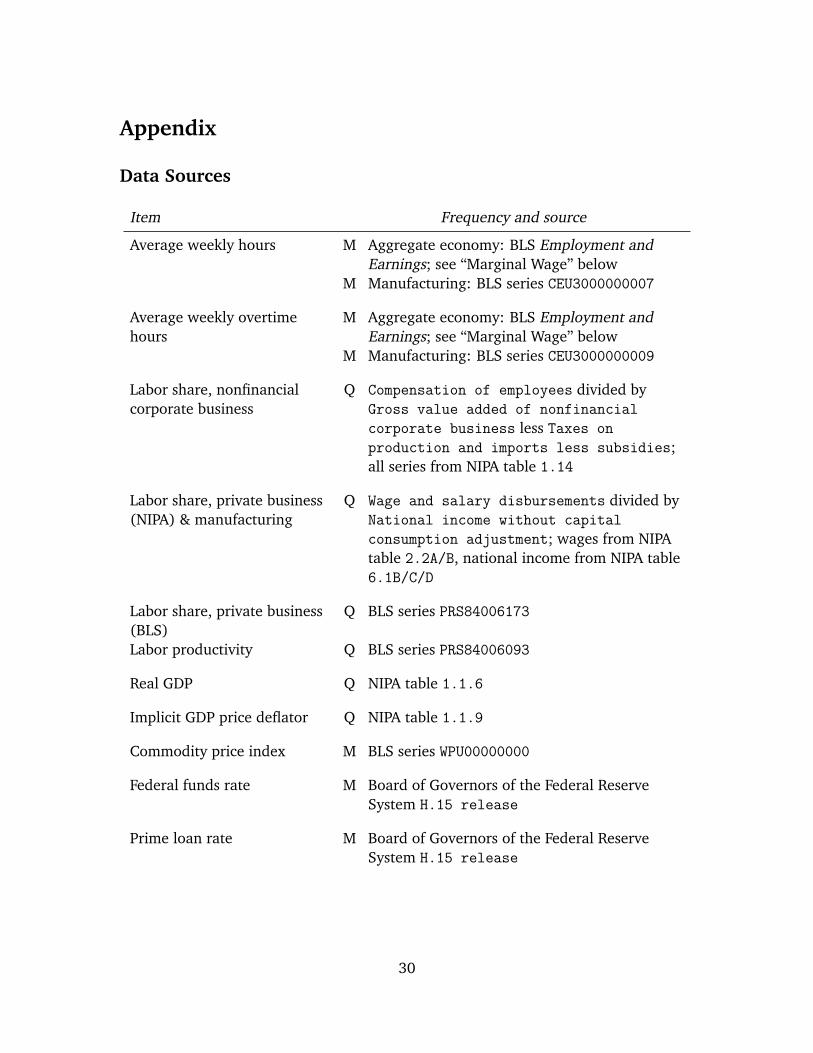
Data Sources

Item Frequency and source

Average weekly hours M Aggregate economy: BLS Employment andEarnings; see “Marginal Wage” below

M Manufacturing: BLS series CEU3000000007

Average weekly overtimehours

M Aggregate economy: BLS Employment andEarnings; see “Marginal Wage” below

M Manufacturing: BLS series CEU3000000009

Labor share, nonfinancialcorporate business

Q Compensation of employees divided byGross value added of nonfinancialcorporate business less Taxes onproduction and imports less subsidies;all series from NIPA table 1.14

Labor share, private business(NIPA) & manufacturing

Q Wage and salary disbursements divided byNational income without capitalconsumption adjustment; wages from NIPAtable 2.2A/B, national income from NIPA table6.1B/C/D

Labor share, private business(BLS)

Q BLS series PRS84006173

Labor productivity Q BLS series PRS84006093

Real GDP Q NIPA table 1.1.6

Implicit GDP price deflator Q NIPA table 1.1.9

Commodity price index M BLS series WPU00000000

Federal funds rate M Board of Governors of the Federal ReserveSystem H.15 release

Prime loan rate M Board of Governors of the Federal ReserveSystem H.15 release

30

Seasonal Adjustment

Both the Current Population Survey (CPS) and Current Employment Statistics (CES)

surveys ask respondents to report actual hours worked during the week of the month

containing the twelfth. Two holidays, Easter and Labor day, periodically fall during the

reference week. When one of these holidays occurs during the reference week, actual

hours worked falls substantially. However, because there this pattern is not regular,

the seasonally-adjusted series published by the Bureau of Labor Statistics (BLS) do not

account for this reference-week holiday effect.

We seasonally adjust the CPS data we construct on employment and average hours

for all workers in the aggregate economy using use the Census Bureau’s X-12-ARIMA

program. We allow the program to remove all large outliers from the final seasonally-

adjusted series. Because the seasonally-adjusted series on production workers in man-

ufacturing are seasonally adjusted at a highly-disaggregated level, we do not perform

our own seasonal adjustment. Instead, we use X-12-ARIMA to identify outliers from

the seasonally-adjusted series and remove the outlier component from the seasonally-

adjusted series.

Average Markup

We construct measures of the price-average cost markup as the inverse of the labor

share. Details of the data are provided in the table above.

For the private business sector using BLS data, the markup is 100 divided by the

index of labor share. For the private business sector using national income and product

accounts (NIPA) data, the markup is wage and salary disbursements divided by national

income without capital consumption adjustment. The markup in manufacturing is

constructed analogously to NIPA private business. Finally, the markup for nonfinancial

corporate business is constructed from the NIPA by dividing compensation of employees

by gross value less taxes on production and imports less subsidies.

Economy-Wide Hours Data

Data on the distribution of hours for civilian workers come from the BLS’s monthly

Employment and Earnings publication. We use three categories of data: persons at

work by hours worked, total persons at work, and average hours worked by persons at

31

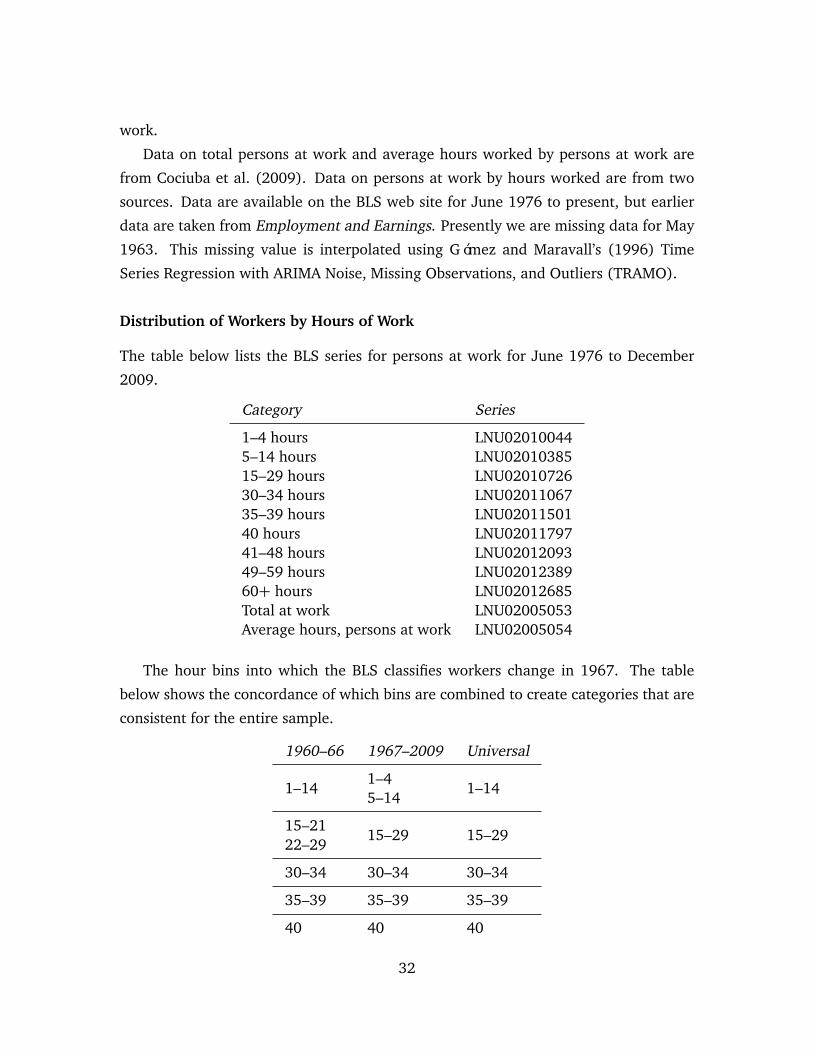
work.

Data on total persons at work and average hours worked by persons at work are

from Cociuba et al. (2009). Data on persons at work by hours worked are from two

sources. Data are available on the BLS web site for June 1976 to present, but earlier

data are taken from Employment and Earnings. Presently we are missing data for May

1963. This missing value is interpolated using Gómez and Maravall’s (1996) Time

Series Regression with ARIMA Noise, Missing Observations, and Outliers (TRAMO).

Distribution of Workers by Hours of Work

The table below lists the BLS series for persons at work for June 1976 to December

2009.

Category Series

1–4 hours LNU020100445–14 hours LNU0201038515–29 hours LNU0201072630–34 hours LNU0201106735–39 hours LNU0201150140 hours LNU0201179741–48 hours LNU0201209349–59 hours LNU0201238960+ hours LNU02012685Total at work LNU02005053Average hours, persons at work LNU02005054

The hour bins into which the BLS classifies workers change in 1967. The table

below shows the concordance of which bins are combined to create categories that are

consistent for the entire sample.

1960–66 1967–2009 Universal

1–141–4

1–145–14

15–2115–29 15–29

22–29

30–34 30–34 30–34

35–39 35–39 35–39

40 40 40

32

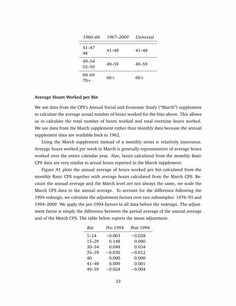
1960–66 1967–2009 Universal

41–4741–48 41–48

48

49–5449–59 49–59

55–59

60–6960+ 60+

70+

Average Hours Worked per Bin

We use data from the CPS’s Annual Social and Economic Study (“March”) supplement

to calculate the average actual number of hours worked for the bins above. This allows

us to calculate the total number of hours worked and total overtime hours worked.

We use data from the March supplement rather than monthly data because the annual

supplement data are available back to 1962.

Using the March supplement instead of a monthly series is relatively innocuous.

Average hours worked per week in March is generally representative of average hours

worked over the entire calendar year. Also, hours calculated from the monthly Basic

CPS data are very similar to actual hours reported in the March supplement.

Figure A1 plots the annual average of hours worked per bin calculated from the

monthly Basic CPS together with average hours calculated from the March CPS. Be-

cause the annual average and the March level are not always the same, we scale the

March CPS data to the annual average. To account for the difference following the

1994 redesign, we calculate the adjustment factors over two subsamples: 1976–93 and

1994–2009. We apply the pre-1994 factors to all data before the redesign. The adjust-

ment factor is simply the difference between the period average of the annual average

and of the March CPS. The table below reports the mean adjustment.

Bin Pre-1994 Post-1994

1–14 −0.063 −0.02815–29 0.148 0.08030–34 0.048 0.03435–39 −0.030 −0.01240 0.000 0.00041–48 0.009 0.00149–59 −0.024 −0.004

33

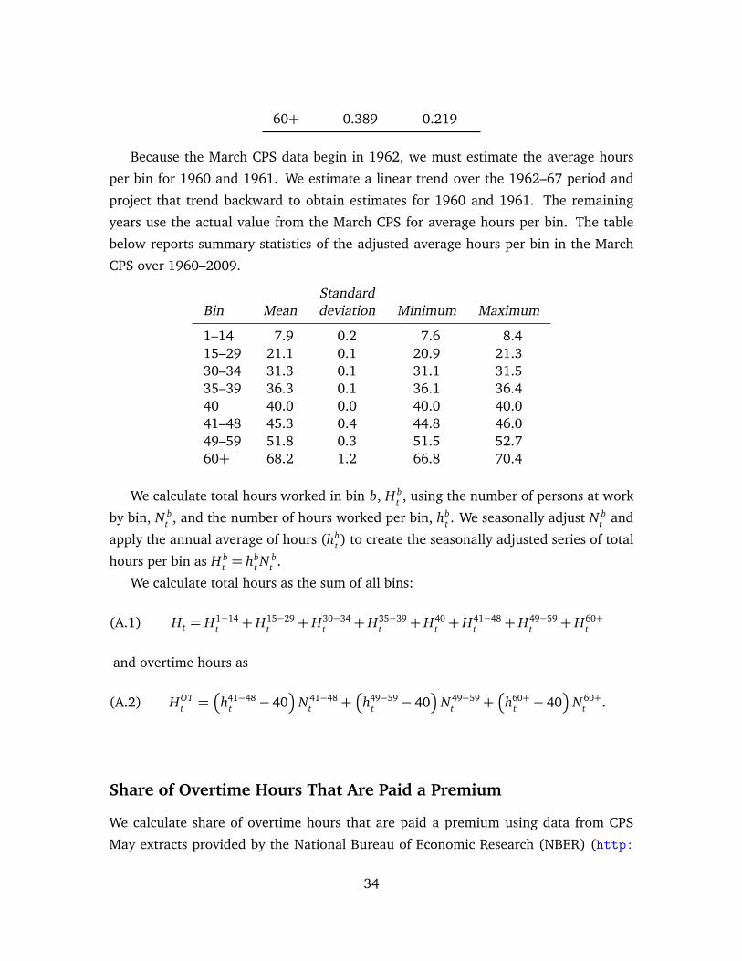
60+ 0.389 0.219

Because the March CPS data begin in 1962, we must estimate the average hours

per bin for 1960 and 1961. We estimate a linear trend over the 1962–67 period and

project that trend backward to obtain estimates for 1960 and 1961. The remaining

years use the actual value from the March CPS for average hours per bin. The table

below reports summary statistics of the adjusted average hours per bin in the March

CPS over 1960–2009.

StandardBin Mean deviation Minimum Maximum

1–14 7.9 0.2 7.6 8.415–29 21.1 0.1 20.9 21.330–34 31.3 0.1 31.1 31.535–39 36.3 0.1 36.1 36.440 40.0 0.0 40.0 40.041–48 45.3 0.4 44.8 46.049–59 51.8 0.3 51.5 52.760+ 68.2 1.2 66.8 70.4

We calculate total hours worked in bin b, H bt , using the number of persons at work

by bin, N bt , and the number of hours worked per bin, hb

t . We seasonally adjust N bt and

apply the annual average of hours (hbt ) to create the seasonally adjusted series of total

hours per bin as H bt = hb

t N bt .

We calculate total hours as the sum of all bins:

(A.1) Ht = H1−14t +H15−29

t +H30−34t +H35−39

t +H40t +H41−48

t +H49−59t +H60+

t

and overtime hours as

(A.2) HOTt =

�

h41−48t − 40

�

N 41−48t +

�

h49−59t − 40

�

N 49−59t +

�

h60+t − 40

�

N 60+t .

Share of Overtime Hours That Are Paid a Premium

We calculate share of overtime hours that are paid a premium using data from CPS

May extracts provided by the National Bureau of Economic Research (NBER) (http:

34

//www.nber.org/data/cps_may.html). The overtime variable (x174) is a dummy for

whether an individual receives higher pay for work exceeding 40 hours in a week.

(Note that the value 0 indicates that a worker received premium pay.)

We drop all individuals that do not report total hours (variable x28). We calculate

overtime hours as hours worked at primary job (variable x182) less 40 when this is

reported; otherwise, overtime hours is calculated as total hours worked less 40. An

individual’s paid overtime hours is the product of overtime hours and the indicator

for whether overtime hours are paid a premium. We aggregate overtime hours, paid

overtime hours, and total hours by year using the individual sampling weights (variable

x80). For a given year, the share of overtime that is paid a premium is the ratio of paid

overtime hours to total overtime hours.

Longitudinal Population Database

These data were constructed by Nekarda’s (2009) by matching respondents from the

monthly CPS.

(More details to come.)

35

References

Baily, Martin Neil, 1974. “Wages and Employment under Uncertain Demand.” Reviewof Economic Studies 41(1): 37–50.

Baratierri, Alessandro, Susanto Basu, and Peter. Gottschalk, 2010. “Some Evidenceon the Importance of Sticky Wages.” Working paper 16130, National Bureau ofEconomic Research.

Barth, Marvin J. and Valerie A. Ramey, 2002. “The Cost Channel of Monetary Trans-mission.” In NBER Macroeconomics Annual 2001, edited by Ben S. Bernanke andJulio Rotemberg, pp. 199–256. University of Chicago Press.

Basu, Susanto and John G. Fernald, 1997a. “Cyclical Productivity with UnobservedInput Variation.” (5915).

Basu, Susanto and John G. Fernald, 1997b. “Returns to Scale in US Production:Estimates and Implications.” Journal of Political Economy 105(2): 249–83.

Bils, Mark, 1987. “The Cyclical Behavior of Marginal Cost and Price.” AmericanEconomic Review 77(5): 838–55.

Bils, Mark, 2005. “Deducing Markup Cyclicality from Stockout Behavior.” Unpublishedpaper, University of Rochester.

Bils, Mark and James A. Kahn, 2000. “What Inventory Behavior Tells Us About Busi-ness Cycles.” American Economic Review 90(3): 458–81.

Blanchard, Olivier J., 2008. “The State of Macro.” Working Paper 14259, NationalBureau of Economic Research, Cambridge, MA.

Carr, Darrell E., 1986. “Overtime Work: An Expanded View.” Monthly Labor Review109(11): 36–9.

Chirinko, Robert S., 2008. “σ: The Long and Short of It.” Journal of Macroeconomics30(2): 671–86.

Chirinko, Robert S. and Stephen M. Fazzari, 1994. “Economic Fluctuations, MarketPower, and Returns to Scale: Evidence from Firm-Level Data.” Journal of AppliedEconometrics 9(1): 47–69.

Chirinko, Robert S. and Stephen M. Fazzari, 2000. “Market Power and Inflation.”The Review of Economics and Statistics 82(3): 509–513.

Christiano, Lawrence J., Martin Eichenbaum, and Charles L. Evans, 2005. “Nom-inal Rigidities and the Dynamic Effects of A Shock to Monetary Policy.” Journal ofPolitical Economy 113(1): 1–45.

36

Cociuba, Simona, Edward C. Prescott, and Alexander Ueberfeldt, 2009. “U.S.Hours and Productivity Behavior Using CPS Hours Worked Data: 1947-III to 2009-II.” Working paper, Federal Reserve Bank of Dallas.

Cooper, Russell W. and John C. Haltiwanger, 2006. “On the Nature of Capital Ad-justment Costs.” Review of Economic Studies 73(3): 611–33.

Domowitz, Ian R., Glenn Hubbard, and Bruce C. Petersen, 1986. “Business Cyclesand the Relationship between Concentration and Price-Cost Margins.” The RANDJournal of Economics 17(1): 1–17.

Dunlop, John T., 1938. “The Movement of Real and Money Wage Rates.” The Eco-nomic Journal 48(191): 413–34.

Erceg, Christopher J., Dale W. Henderson, and Andrew T. Levin, 2000. “OptimalMonetary Policy with Staggered Wage and Price Contracts.” Journal of MonetaryEconomics 46(2): 281–313.

Francis, Neville and Valerie A. Ramey, 2009. “Measures of per Capita Hours andTheir Implications for the Technology-Hours Debate.” Journal of Money, Credit andBanking 41(6): 1071–97.

Galí, Jordi, 1999. “Technology, Employment, and the Business Cycle: Do TechnologyShocks Explain Aggregate Fluctuations?” American Economic Review 89(1): 249–71.

Galí, Jordi and Mark Gertler, 1999. “Inflation Dynamics: A Structural EconometricAnalysis.” Journal of Monetary Economics 44(2): 195–222.

Galí, Jordi, Mark Gertler, and J. David López-Salido, 2007. “Markups, Gaps, and theWelfare Costs of Business Fluctuations.” Review of Economics and Statistics 89(1):44–59.

Gómez, Victor and Agustín Maravall, 1996. “Programs TRAMO and SEATS: Instruc-tions for the User.” Working paper 9628, Banco de España.

Goodfriend, Marvin and Robert G. King, 1997. “The New Neoclassical Synthesisand the Role of Monetary Policy.” In NBER Macroeconomics Annual 1997, edited byBen S. Bernanke and Julio Rotemberg, pp. 231–83. MIT Press.

Gordon, Robert J., 1981. “Output Fluctuations and Gradual Price Adjustment.” Jour-nal of Economic Literature 19(2): 493–530.

Gourio, François and Anil K. Kashyap, 2007. “Investment Spikes: New Facts and aGeneral Equilibrium Exploration.” Journal of Monetary Economics 54(Supplement1): 1–22.

37

Hall, Robert E., 1980. “Employment Fluctuations and Wage Rigidity.” Brookings Pa-pers on Economic Activity 1: 91–123.

Hall, Robert E., 2004. “Measuring Factor Adjustment Cost.” Quarterly Journal ofEconomics 119(3): 899–927.

Hamermesh, Daniel S., 2006. “Overtime Laws and the Margins of Work Timing.”Unpublished paper, University of Texas, Austin.

Hamermesh, Daniel S. and Gerard A. Pfann, 1996. “Adjustment Costs in FactorDemand.” Journal of Economic Literature 34(3): 1264–92.

Hirsch, Barry T., 2005. “Why Do Part-Time Workers Earn Less? The Role of Workerand Job Skills.” Industrial and Labor Relations Review 58(4): 525–51.

Jaimovich, Nir and Max Floetotto, 2008. “Firm Dynamics, Markup Variations, andthe Business Cycle.” Journal of Monetary Economics 55(7): 1238–52.

Keynes, John Maynard, 1936. The General Theory of Interest, Employment andMoney. London.

Khan, Aubhik and Julia K. Thomas, 2007. “Inventories and the Business Cycle: AnEquilibrium Analysis of (S, s) Policies.” American Economic Review 97(4): 1165–88.

Levin, Andrew T., Alexei Onatski, John C. Williams, and Noah Willams, 2005.“Monetary Policy under Uncertainty in Micro-Founded Macroeconomic Models.” InNBER Macroeconomics Annual 2005, pp. 229–287. The University of Chicago Press.

Mazumder, Sandeep, 2010. “The Price-Marginal Cost Markup and its Determinants inU.S. Manufacturing.” Unpublished paper, Wake Forest University.

Nekarda, Christopher J., 2009. “A Longitudinal Analysis of the Current PopulationSurvey: Assessing the Cyclical Bias of Geographic Mobility.” Unpublished paper,Federal Reserve Board of Governors.

Nekarda, Christopher J. and Valerie A. Ramey, 2010. “Industry Evidence on the Ef-fects of Government Spending.” Working paper, University of California, San Diego.

Perotti, Roberto, 2008. “In Search of the Transmission Mechanism of Fiscal Policy.”In NBER Macroeconomics Annual 2007, edited by Daron Acemoglu, Kenneth Rogoff,and Michael Woodford, pp. 169–226. University of Chicago Press.

Phelps, Edmund S., 1968. “Money-Wage Dynamics and Labor Market Equilibrium.”Journal of Political Economy 76(4): 678–711.

Ramey, Valerie A., 1991. “Discussion of ‘Markups and the Business Cycle’.” In NBERMacroeconomics Annual 1991, edited by Olivier Jean Blanchard and Stanley Fischer,pp. 134–40. MIT Press.

38

Ravenna, Federico and Carl E. Walsh, 2006. “Optimal Monetary Policy with the CostChannel.” Journal of Monetary Economics 53(2): 199–216.

Rotemberg, Julio J., 1982. “Monopolistic Price Adjustment and Aggregate Output.”Journal of Political Economy 49(4): 517–31.

Rotemberg, Julio J. and Michael Woodford, 1991. “Markups and the Business Cy-cle.” In NBER Macroeconomics Annual 1991, edited by Olivier Jean Blanchard andStanley Fischer, pp. 63–129. MIT Press.

Rotemberg, Julio J. and Michael Woodford, 1992. “Oligopolistic Pricing and theEffects of Aggregate Demand on Economic Activity.” Journal of Political Economy100(6): 1153–207.

Rotemberg, Julio J. and Michael Woodford, 1999. “The Cyclical Behavior of Pricesand Costs.” In Handbook of Macroeconomics, edited by John B. Taylor and MichaelWoodford, pp. 1051–135. Elsevier.

Sbordone, Argia, 2002. “Price and Unit Labor Costs: A New Test of Price Stickiness.”Journal of Monetary Economics 49(2): 265–92.

Shea, John, 1993. “Do Supply Curves Slope up?” Quarterly Journal of Economics108(1): 1–32.

Smets, Frank and Rafael Wouters, 2003. “An Estimated Dynamic Stochastic GeneralEquilibrium Model of the Euro Area.” Journal of the European Economic Association1(5): 1123–75.

Smets, Frank and Rafael Wouters, 2007. “Shocks and Frictions in US Business Cycles:A Bayesian DSGE Approach.” American Economic Review 97(3): 586–606.

Tarshis, Lorie, 1939. “Changes in Real and Money Wages.” The Economic Journal49(193): 150–4.

Taylor, Daniel E. and Edward S. Sekscenski, 1982. “Workers on Long Schedules,Single and Multiple Jobholders.” Monthly Labor Review 105(5): 47–53.

Taylor, John B., 1980. “Aggregate Dynamics and Staggered Contracts.” Journal ofPolitical Economy 88(1): 1–23.

Trejo, Stephen J., 1991. “The Effects of Overtime Pay Regulation on Worker Compen-sation.” American Economic Review 81(4): 719–40.

Wetzel, James R., 1966. “Overtime Hours and Premium Pay.” Monthly Labor Review89(9): 973–7.

Woodford, Michael, 2003. Interest and Prices: Foundations of A Theory of MonetaryPolicy. Princeton, N.J.: Princeton University Press.

39

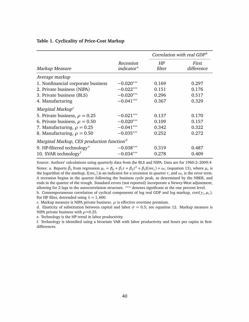
Table 1. Cyclicality of Price-Cost Markup

Correlation with real GDP b

Recession HP FirstMarkup Measure indicator a filter difference

Average markup1. Nonfinancial corporate business −0.020∗∗∗ 0.169 0.2972. Private business (NIPA) −0.022∗∗∗ 0.151 0.1763. Private business (BLS) −0.020∗∗∗ 0.296 0.5174. Manufacturing −0.041∗∗∗ 0.367 0.329

Marginal Markup c

5. Private business, ρ = 0.25 −0.021∗∗∗ 0.137 0.1706. Private business, ρ = 0.50 −0.020∗∗∗ 0.109 0.1577. Manufacturing, ρ = 0.25 −0.041∗∗∗ 0.342 0.3228. Manufacturing, ρ = 0.50 −0.035∗∗∗ 0.252 0.272

Marginal Markup, CES production functiond

9. HP-filtered technology e −0.038∗∗∗ 0.319 0.48710. SVAR technology f −0.034∗∗∗ 0.278 0.409

Source: Authors’ calculations using quarterly data from the BLS and NIPA. Data are for 1960:2–2009:4Notes: a. Reports bβ3 from regression µt = β0 + β1 t + β2 t2 + β3I(rect) +ωt (equation 13), where µt isthe logarithm of the markup, I(rect) is an indicator for a recession in quarter t, and ωt is the error term.A recession begins in the quarter following the business cycle peak, as determined by the NBER, andends in the quarter of the trough. Standard errors (not reported) incorporate a Newey-West adjustment,allowing for 2 lags in the autocorrelation structure. *** denotes significant at the one percent level.b. Contemporaneous correlation of cyclical components of log real GDP and log markup, corr(yt ,µt).For HP filter, detrended using λ= 1,600.c. Markup measure is NIPA private business. ρ is effective overtime premium.d. Elasticity of substitution between capital and labor σ = 0.5; see equation 12. Markup measure isNIPA private business with ρ=0.25.e. Technology is the HP trend in labor productivity.f. Technology is identified using a bivariate VAR with labor productivity and hours per capita in first-differences.

40

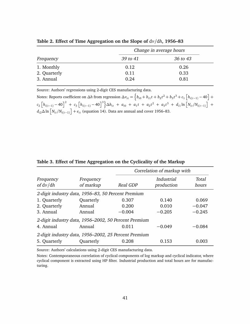
Table 2. Effect of Time Aggregation on the Slope of dv/dh, 1956–83

Change in average hours

Frequency 39 to 41 36 to 43

1. Monthly 0.12 0.262. Quarterly 0.11 0.333. Annual 0.24 0.81

Source: Authors’ regressions using 2-digit CES manufacturing data.

Notes: Reports coefficient on ∆h from regression ∆vi t =n

bi0 + bi1 t + b2 t2 + b3 t3 + c1

�

hi(t−1) − 40�

+

c2

�

hi(t−1) − 40�2+ c3

�

hi(t−1) − 40�3o

∆hi t + ai0 + a1 t + a2 t2 + a3 t3 + di1 ln�

Ni t/Ni(t−1)

�

+

di2∆ ln�

Ni t/Ni(t−1)

�

+ ei t (equation 14). Data are annual and cover 1956–83.

Table 3. Effect of Time Aggregation on the Cyclicality of the Markup

Correlation of markup with

Frequency Frequency Industrial Totalof dv/dh of markup Real GDP production hours

2-digit industry data, 1956–83, 50 Percent Premium1. Quarterly Quarterly 0.307 0.140 0.0692. Quarterly Annual 0.200 0.010 −0.0473. Annual Annual −0.004 −0.205 −0.245

2-digit industry data, 1956–2002, 50 Percent Premium4. Annual Annual 0.011 −0.049 −0.084

2-digit industry data, 1956–2002, 25 Percent Premium5. Quarterly Quarterly 0.208 0.153 0.003

Source: Authors’ calculations using 2-digit CES manufacturing data.Notes: Contemporaneous correlation of cyclical components of log markup and cyclical indicator, wherecyclical component is extracted using HP filter. Industrial production and total hours are for manufac-turing.

41

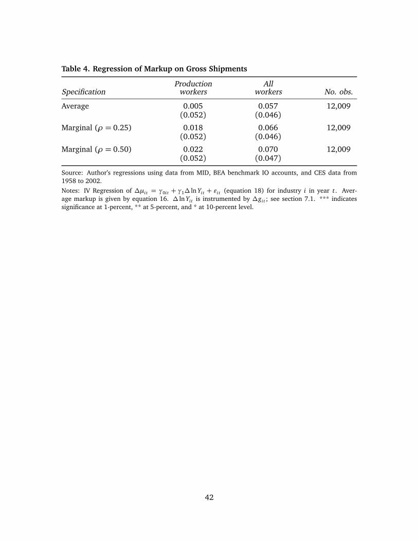
Table 4. Regression of Markup on Gross Shipments

Production AllSpecification workers workers No. obs.

Average 0.005 0.057 12,009(0.052) (0.046)

Marginal (ρ = 0.25) 0.018 0.066 12,009(0.052) (0.046)

Marginal (ρ = 0.50) 0.022 0.070 12,009(0.052) (0.047)

Source: Author’s regressions using data from MID, BEA benchmark IO accounts, and CES data from1958 to 2002.Notes: IV Regression of ∆µi t = γ0i t + γ1∆ ln Yi t + εi t (equation 18) for industry i in year t. Aver-age markup is given by equation 16. ∆ ln Yi t is instrumented by ∆gi t ; see section 7.1. *** indicatessignificance at 1-percent, ** at 5-percent, and * at 10-percent level.

42

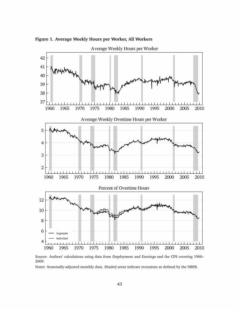
Figure 1. Average Weekly Hours per Worker, All Workers

37

38

39

40

41

42

1960 1965 1970 1975 1980 1985 1990 1995 2000 2005 2010

Average Weekly Hours per Worker

2

3

4

5

1960 1965 1970 1975 1980 1985 1990 1995 2000 2005 2010

Average Weekly Overtime Hours per Worker

4

6

8

10

12

1960 1965 1970 1975 1980 1985 1990 1995 2000 2005 2010

Aggregate

Individual

Percent of Overtime Hours

Source: Authors’ calculations using data from Employment and Earnings and the CPS covering 1960–2009.Notes: Seasonally-adjusted monthly data. Shaded areas indicate recessions as defined by the NBER.

43

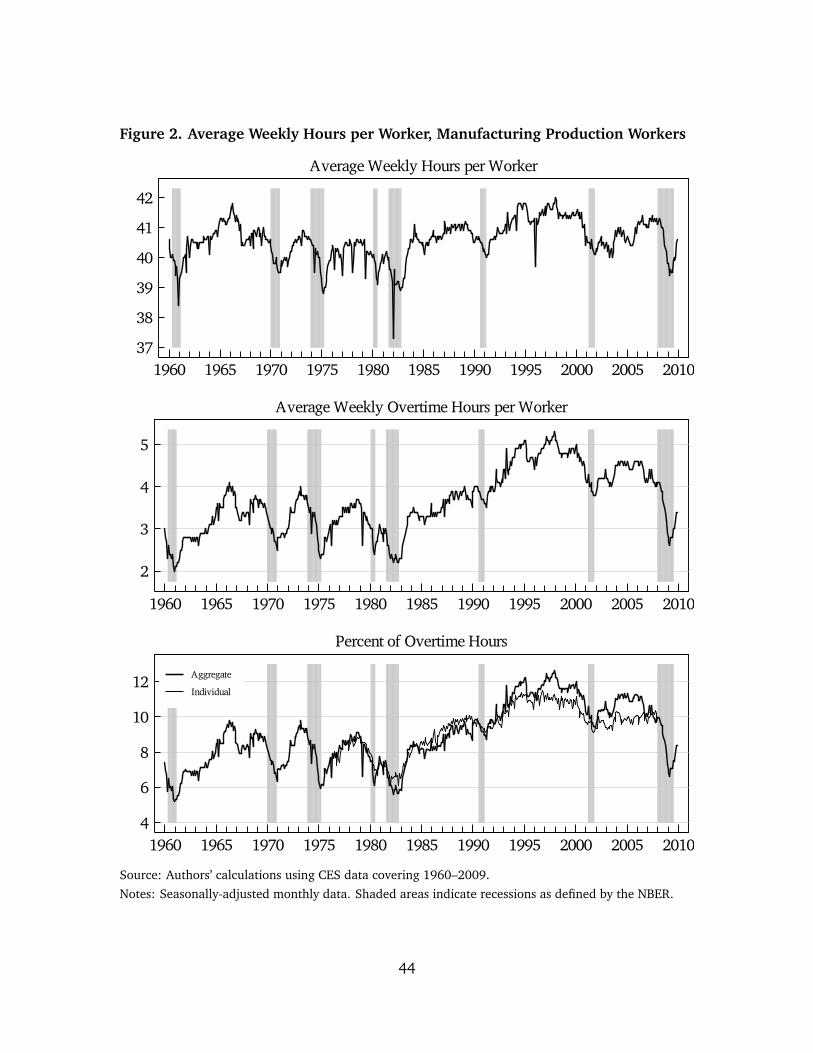
Figure 2. Average Weekly Hours per Worker, Manufacturing Production Workers

37

38

39

40

41

42

1960 1965 1970 1975 1980 1985 1990 1995 2000 2005 2010

Average Weekly Hours per Worker

2

3

4

5

1960 1965 1970 1975 1980 1985 1990 1995 2000 2005 2010

Average Weekly Overtime Hours per Worker

4

6

8

10

12

1960 1965 1970 1975 1980 1985 1990 1995 2000 2005 2010

Aggregate

Individual

Percent of Overtime Hours

Source: Authors’ calculations using CES data covering 1960–2009.Notes: Seasonally-adjusted monthly data. Shaded areas indicate recessions as defined by the NBER.

44

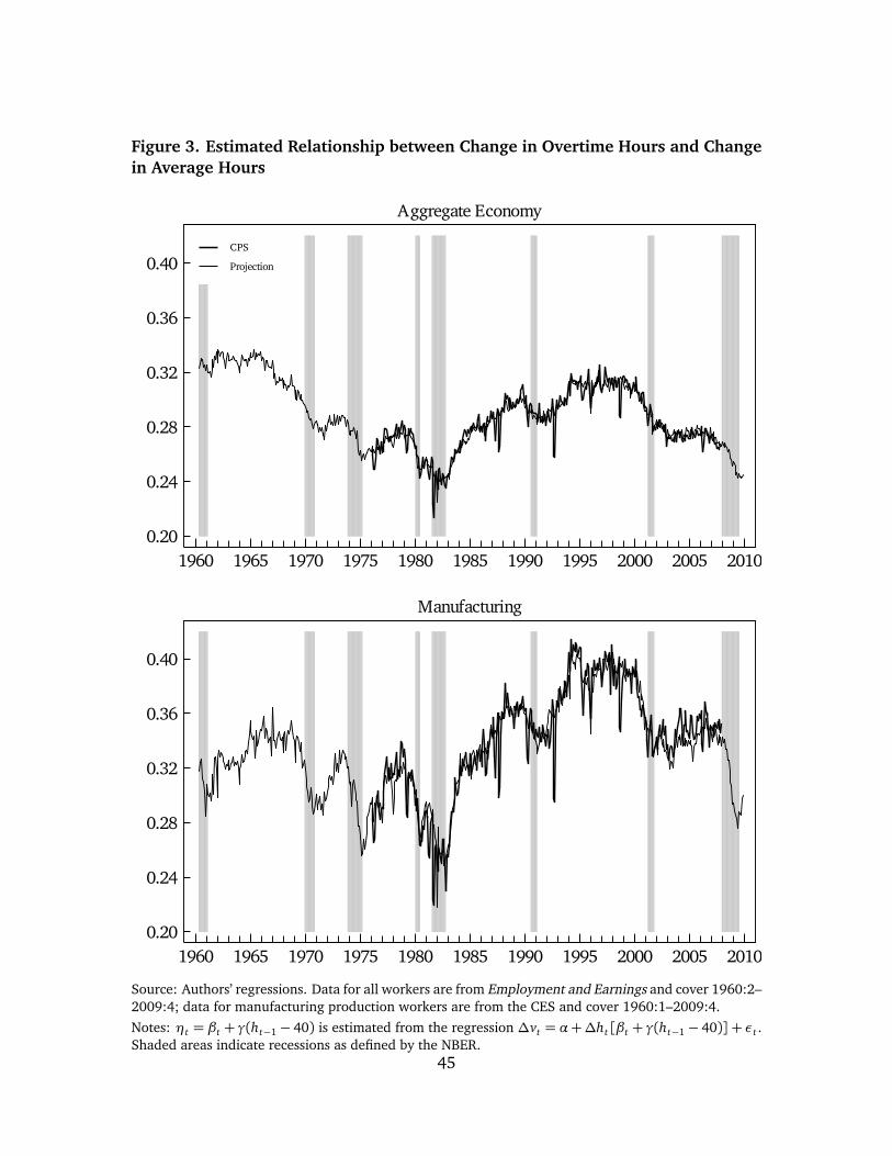
Figure 3. Estimated Relationship between Change in Overtime Hours and Changein Average Hours

0.20

0.24

0.28

0.32

0.36

0.40

1960 1965 1970 1975 1980 1985 1990 1995 2000 2005 2010

CPS

Projection

Aggregate Economy

0.20

0.24

0.28

0.32

0.36

0.40

1960 1965 1970 1975 1980 1985 1990 1995 2000 2005 2010

Manufacturing

Source: Authors’ regressions. Data for all workers are from Employment and Earnings and cover 1960:2–2009:4; data for manufacturing production workers are from the CES and cover 1960:1–2009:4.Notes: ηt = βt + γ(ht−1 − 40) is estimated from the regression ∆vt = α+∆ht[βt + γ(ht−1 − 40)] + εt .Shaded areas indicate recessions as defined by the NBER.

45

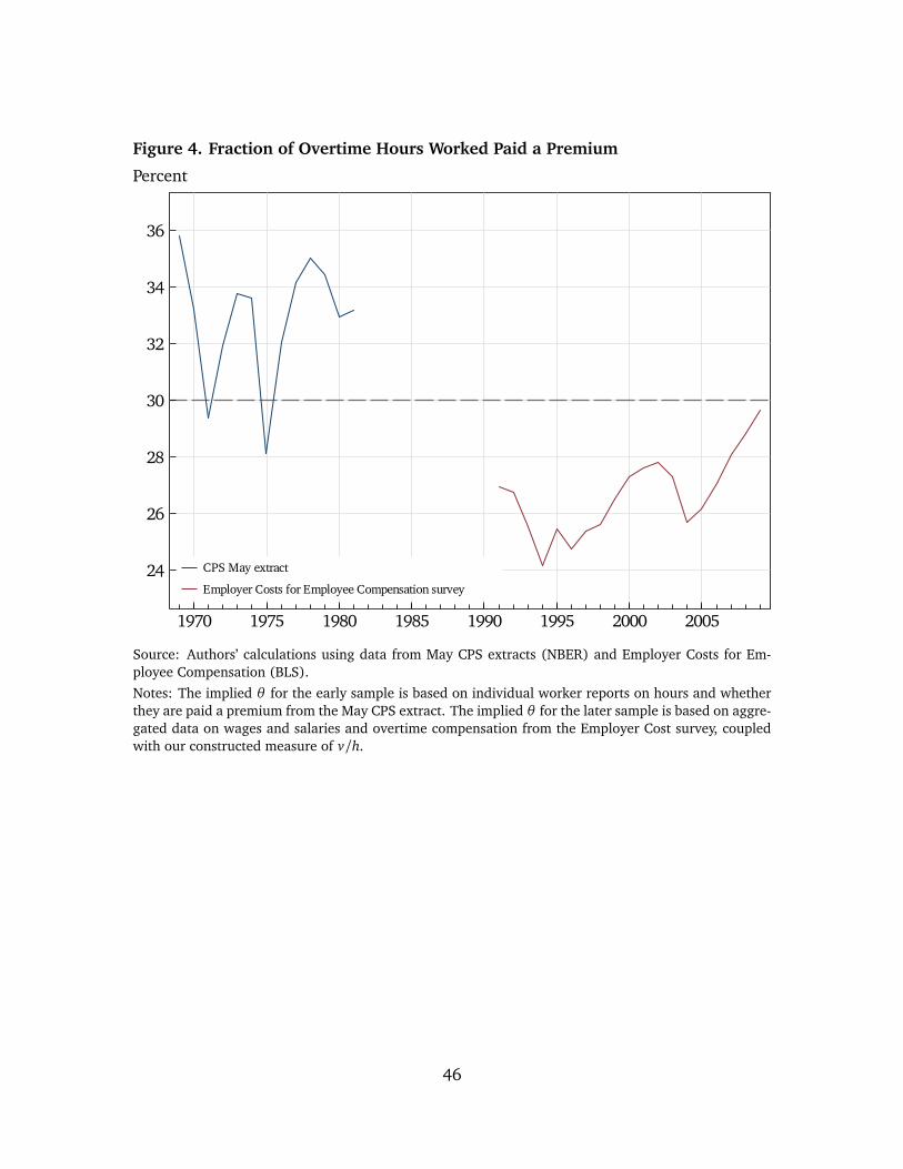
Figure 4. Fraction of Overtime Hours Worked Paid a Premium

Percent

24

26

28

30

32

34

36

1970 1975 1980 1985 1990 1995 2000 2005

CPS May extract

Employer Costs for Employee Compensation survey

Source: Authors’ calculations using data from May CPS extracts (NBER) and Employer Costs for Em-ployee Compensation (BLS).Notes: The implied θ for the early sample is based on individual worker reports on hours and whetherthey are paid a premium from the May CPS extract. The implied θ for the later sample is based on aggre-gated data on wages and salaries and overtime compensation from the Employer Cost survey, coupledwith our constructed measure of v/h.

46

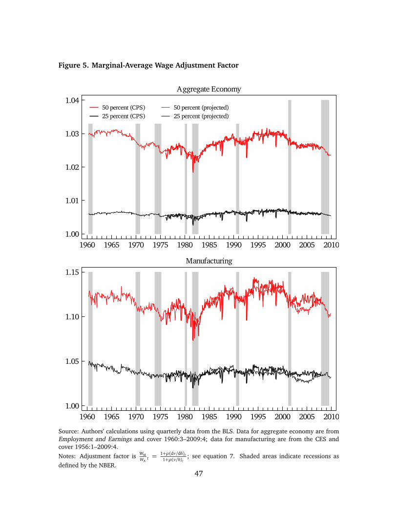
Figure 5. Marginal-Average Wage Adjustment Factor

1.00

1.01

1.02

1.03

1.04

1960 1965 1970 1975 1980 1985 1990 1995 2000 2005 2010

50 percent (CPS) 50 percent (projected)25 percent (CPS) 25 percent (projected)

Aggregate Economy

1.00

1.05

1.10

1.15

1960 1965 1970 1975 1980 1985 1990 1995 2000 2005 2010

Manufacturing

Source: Authors’ calculations using quarterly data from the BLS. Data for aggregate economy are fromEmployment and Earnings and cover 1960:3–2009:4; data for manufacturing are from the CES andcover 1956:1–2009:4.Notes: Adjustment factor is WM

WAt =

1+ρ(dv/dh)t1+ρ(v/h)t

; see equation 7. Shaded areas indicate recessions asdefined by the NBER.

47

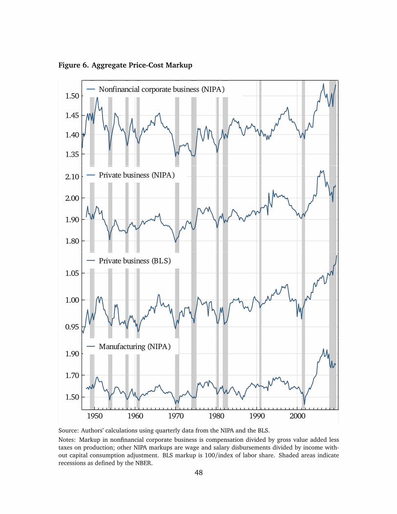
Figure 6. Aggregate Price-Cost Markup

1.35

1.40

1.45

1.50Nonfinancial corporate business (NIPA)

1.80

1.90

2.00

2.10 Private business (NIPA)

0.95

1.00

1.05

Private business (BLS)

1.50

1.70

1.90

1950 1960 1970 1980 1990 2000

Manufacturing (NIPA)

Source: Authors’ calculations using quarterly data from the NIPA and the BLS.Notes: Markup in nonfinancial corporate business is compensation divided by gross value added lesstaxes on production; other NIPA markups are wage and salary disbursements divided by income with-out capital consumption adjustment. BLS markup is 100/index of labor share. Shaded areas indicaterecessions as defined by the NBER.

48

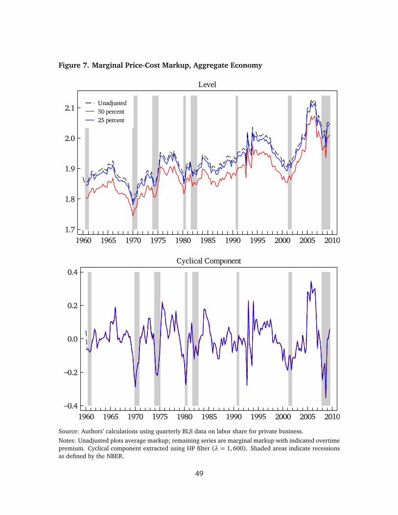
Figure 7. Marginal Price-Cost Markup, Aggregate Economy

1.7

1.8

1.9

2.0

2.1

1960 1965 1970 1975 1980 1985 1990 1995 2000 2005 2010

Unadjusted50 percent25 percent

Level

−0.4

−0.2

0.0

0.2

0.4

1960 1965 1970 1975 1980 1985 1990 1995 2000 2005 2010

Cyclical Component

Source: Authors’ calculations using quarterly BLS data on labor share for private business.Notes: Unadjusted plots average markup; remaining series are marginal markup with indicated overtimepremium. Cyclical component extracted using HP filter (λ = 1, 600). Shaded areas indicate recessionsas defined by the NBER.

49

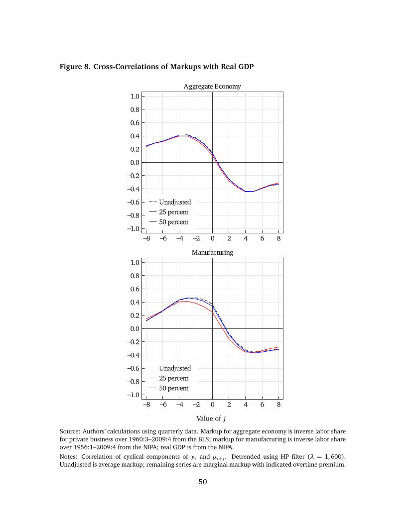
Figure 8. Cross-Correlations of Markups with Real GDP

−1.0

−0.8

−0.6

−0.4

−0.2

0.0

0.2

0.4

0.6

0.8

1.0

−8 −6 −4 −2 0 2 4 6 8

Unadjusted25 percent50 percent

Aggregate Economy

−1.0

−0.8

−0.6

−0.4

−0.2

0.0

0.2

0.4

0.6

0.8

1.0

−8 −6 −4 −2 0 2 4 6 8

Unadjusted25 percent50 percent

Manufacturing

Value of j

Source: Authors’ calculations using quarterly data. Markup for aggregate economy is inverse labor sharefor private business over 1960:3–2009:4 from the BLS; markup for manufacturing is inverse labor shareover 1956:1–2009:4 from the NIPA; real GDP is from the NIPA.Notes: Correlation of cyclical components of yt and µt+ j . Detrended using HP filter (λ = 1, 600).Unadjusted is average markup; remaining series are marginal markup with indicated overtime premium.

50

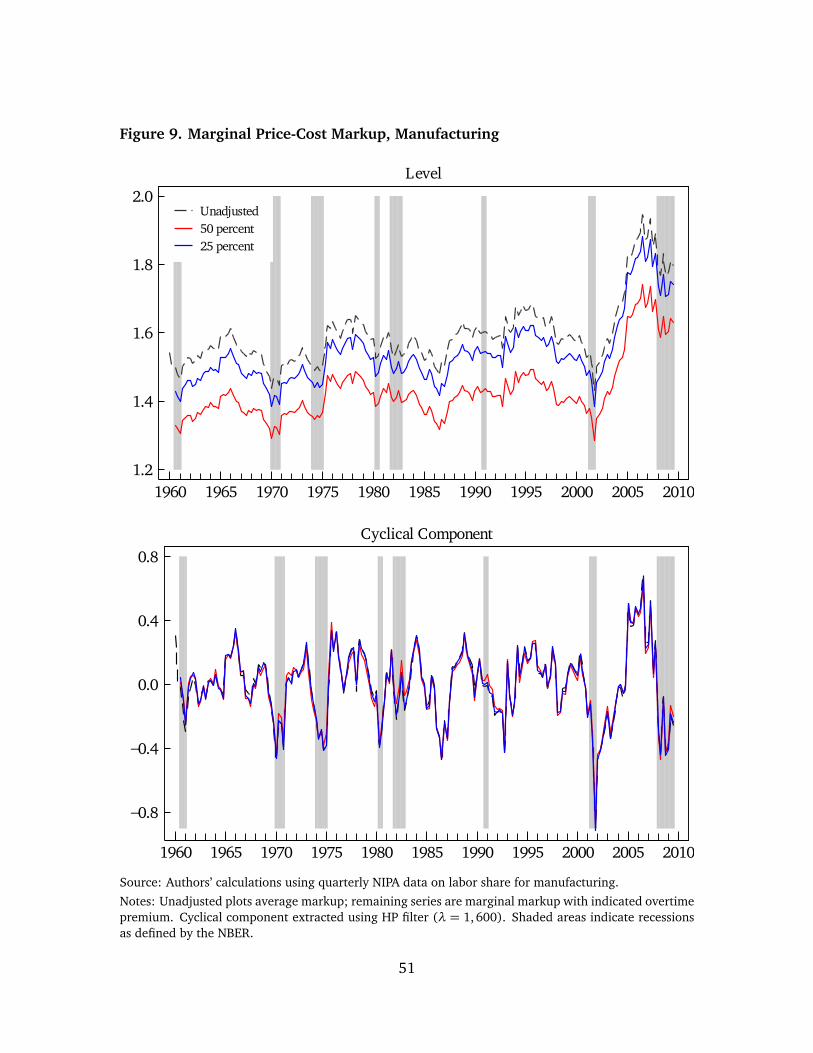
Figure 9. Marginal Price-Cost Markup, Manufacturing

1.2

1.4

1.6

1.8

2.0

1960 1965 1970 1975 1980 1985 1990 1995 2000 2005 2010

Unadjusted50 percent25 percent

Level

−0.8

−0.4

0.0

0.4

0.8

1960 1965 1970 1975 1980 1985 1990 1995 2000 2005 2010

Cyclical Component

Source: Authors’ calculations using quarterly NIPA data on labor share for manufacturing.Notes: Unadjusted plots average markup; remaining series are marginal markup with indicated overtimepremium. Cyclical component extracted using HP filter (λ = 1, 600). Shaded areas indicate recessionsas defined by the NBER.

51

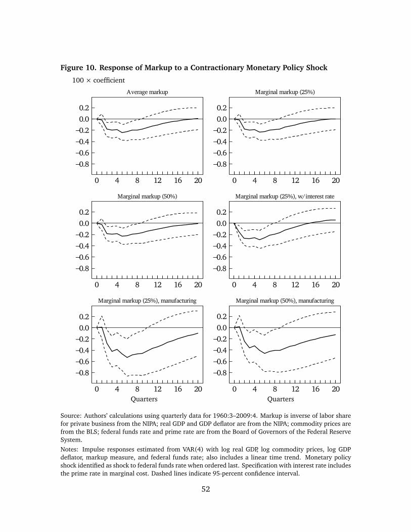
Figure 10. Response of Markup to a Contractionary Monetary Policy Shock

100 × coefficient

−0.8−0.6−0.4−0.2

0.00.2

0 4 8 12 16 20

Average markup

−0.8−0.6−0.4−0.2

0.00.2

0 4 8 12 16 20

Marginal markup (25%)

−0.8−0.6−0.4−0.2

0.00.2

0 4 8 12 16 20

Marginal markup (50%)

−0.8−0.6−0.4−0.2

0.00.2

0 4 8 12 16 20

Marginal markup (25%), w/ interest rate

−0.8−0.6−0.4−0.2

0.00.2

0 4 8 12 16 20

Marginal markup (25%), manufacturing

−0.8−0.6−0.4−0.2

0.00.2

0 4 8 12 16 20

Marginal markup (50%), manufacturing

Quarters Quarters

Source: Authors’ calculations using quarterly data for 1960:3–2009:4. Markup is inverse of labor sharefor private business from the NIPA; real GDP and GDP deflator are from the NIPA; commodity prices arefrom the BLS; federal funds rate and prime rate are from the Board of Governors of the Federal ReserveSystem.Notes: Impulse responses estimated from VAR(4) with log real GDP, log commodity prices, log GDPdeflator, markup measure, and federal funds rate; also includes a linear time trend. Monetary policyshock identified as shock to federal funds rate when ordered last. Specification with interest rate includesthe prime rate in marginal cost. Dashed lines indicate 95-percent confidence interval.

52

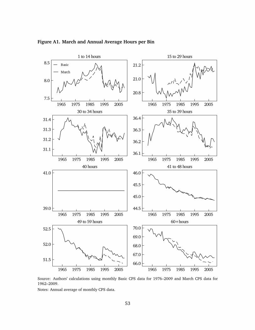
Figure A1. March and Annual Average Hours per Bin

7.5

8.0

8.5

1965 1975 1985 1995 2005

Basic

March

1 to 14 hours

20.8

21.0

21.2

1965 1975 1985 1995 2005

15 to 29 hours

31.1

31.2

31.3

31.4

1965 1975 1985 1995 2005

30 to 34 hours

36.1

36.2

36.3

36.4

1965 1975 1985 1995 2005

35 to 39 hours

39.0

41.0

1965 1975 1985 1995 2005

40 hours

44.5

45.0

45.5

46.0

1965 1975 1985 1995 2005

41 to 48 hours

51.5

52.0

52.5

1965 1975 1985 1995 2005

49 to 59 hours

66.0

67.0

68.0

69.0

70.0

1965 1975 1985 1995 2005

60+ hours

Source: Authors’ calculations using monthly Basic CPS data for 1976–2009 and March CPS data for1962–2009.Notes: Annual average of monthly CPS data.

53