138

American Economic Journal: Microeconomics 2014, 6(4): 138–161 http://dx.doi.org/10.1257/mic.6.4.138

The Control Premium: A Preference for Payoff Autonomy †

By David Owens, Zachary Grossman, and Ryan Fackler *

We document individuals’ willingness to pay to control their own pay-off. Experiment participants choose whether to bet on themselves or on a partner answering a quiz question correctly. Given participants’ beliefs, which we elicit separately, expected-money maximizers would bet on themselves in 56.4 percent of the decisions. However, partici-pants actually bet on themselves in 64.9 percent of their opportunities, reflecting an aggregate control premium. The average participant is willing to sacrifice 8 percent to 15 percent of expected asset earn-ings to retain control. Thus, agents may incur costs to avoid delegat-ing, and studies inferring beliefs from choices may overestimate their results on overconfidence. (JEL C91, D12, D82, D83)

Many people prefer to maintain control over the events that affect their lives. Despite a robust psychological literature on the “Desire for Control,” its eco-

nomic consequences have been largely overlooked.1 To the extent that the feeling of control contributes to subjective well-being (Benjamin et al. 2012), people will pursue it as an objective and be willing to incur costs to retain it.

Thus, a preference for control can influence economic and managerial decisions, in particular, by undermining the willingness to delegate tasks to others. For exam-ple, it might lead an investor to avoid relying on a more skilled financial agent, or an executive to micromanage her subordinates, even if they have more specialized skills. This influence has consequences for our understanding of behavior and wel-fare, and methodological implications for the inference of beliefs from behavior, as has become common in the study of overconfidence, for example.

In this paper, we take a first step at investigating the impact of preferences for control by experimentally measuring the control premium: the monetary cost that

1 Burger and Cooper (1979) argue that a preference for control is a stable personality trait. Individuals who rate highly on their “Desirability of Control” scale are characterized by an affinity for leadership roles and a preference for making their own decisions. Conversely, individuals with low desires for control dislike responsibility, even with respect to their own lives, and they prefer others to make decisions for them. The notion of desirability of control continues to be used in investigations of behavioral patterns and psychological treatments. For example, Burger (1992) depicts the desire for control as an important factor within various phenomena such as achievement, psychological adaptation, stress, or health.

* Owens: Department of Economics, Haverford College, 370 Lancaster Ave, Haverford, PA 19041 (e-mail: dow-ens@haverford.edu); Grossman: Department of Economics, University of California–Santa Barbara, 2127 North Hall, Santa Barbara, CA 93106 (e-mail: grossman@econ.ucsb.edu); Fackler: Department of Economics, University of Pennsylvania, 160 McNeil Building, 3718 Locust Walk, Philadelphia, PA, 19104 (e-mail: fackler@sas.upenn.edu). We are grateful to seminar participants at the 2011 ESA International Meetings, 2011 SEA Meetings, the 2011 ESA North American Regional Meetings, and the 2012 EBEL conference for helpful comments, and to Kent Messer and Jacob Fooks of the University of Delaware for their gracious assistance.

† Go to http://dx.doi.org/10.1257/mic.6.4.138 to visit the article page for additional materials and author disclosure statement(s) or to comment in the online discussion forum.

VoL. 6 No. 4 139owens et al.: the control premium

people are willing to incur in order to retain control over their own payoffs. Each participant took a short quiz, but first made a series of choices between an asset that paid $20 only if she later answered a particular quiz question correctly and one that paid the same amount only if her partner (“Match”) later answered a differ-ent question correctly. Participants retained payoff autonomy by choosing payment contingent on their own correct answer, rather than that of their Match. Importantly, as both choices can only yield $0 or $20, risk attitudes are not confounded with a willingness to pay for control.

The experiment featured two main conditions. In the Choice condition, partici-pants simultaneously previewed a randomly selected question from their own quiz and one from their Match’s quiz. In the same step, they chose the question upon which to risk their contingent payment, without ever being asked to report prob-ability estimates. In three different versions of the Probability and Choice condi-tion, they previewed the questions and, in the same step, reported the probability with which they expected each question to be answered correctly. Next, they chose between the two assets, but without viewing the questions again. Instead, they were shown the likelihoods that they had estimated for each question.

Divorcing the elicitation of beliefs from the asset choice allows us to sepa-rate the influence of (overconfident) beliefs from that of preferences on partici-pants’ decisions.2 We quantify the desire for control by comparing participants’ actual asset choices to those predicted—using reported subjective beliefs—for an expected-money maximizer. First, we make aggregate-level, between-subjects com-parisons, pitting the behavior of the participants in the Choice condition against that predicted using the beliefs of the participants in the Probability and Choice condi-tions, who reported their beliefs before learning of the pending asset choice. Then we measure the control premium at the individual level, comparing within-subject the beliefs and behavior of the participants in the Probability and Choice conditions.

Both methodologies yield evidence of a nontrivial control premium. Participants in the Choice condition staked their earnings on their own performance in 64.9 per-cent of their choices, far in excess of the 56.4 percent of the instances in which self-reliance would be chosen—according to the beliefs expressed in the Probability and Choice conditions—by expected-money maximizers. At the individual level, over 80 percent of our participants follow a cutoff strategy, choosing payoff autonomy if and only if the expected cost is below a fixed level. Preferences for control are heterogeneous. While the modal cutoff is zero, consistent with no control premium, more than 25 percent of the participants exhibit a positive control premium and some exhibit an aversion to control. The average cutoff corresponds to a control premium of $0.62 to $1.19, which amounts to 8 percent to 15 percent of the average earnings from the asset choice. The existence of these cutoffs and the fact that they are frequently nonzero, yet rarely extreme, suggests that the preference for control exerts a consistent, well-behaved, nontrivial influence on delegation decisions.

2 Closely related to our work is that of Charness and Gneezy (2010), who, in part of their study, let participants choose whether to roll a die used to resolve the uncertain return of an asset or to allow the experimenter to do it. However, without eliciting participants’ beliefs about the outcomes of a die rolled by themselves versus the experi-menter, one cannot judge whether participants believed they could influence the outcome more favorably than the experimenter and whether their behavior was consistent with expected payoff maximization given their beliefs.

140 AMERICAN ECONOMIC JOURNAL: MICROECONOMICS NOVEMBER 2014

Participants are likely to have private information about their own knowledge and to have less precise beliefs about others’ performance than about their own. Thus, ambiguity aversion might sway participants to choose a probabilistically inferior asset that depends upon their own success. Rather than viewing ambiguity aversion as a possible confounding factor, we allow that it may contribute to and partially explain the existence of a control premium. To gauge the extent to which this is true, we vary ambiguity across three different Probability and Choice conditions. To accomplish this, we alter the amount of information participants have about their Match and the difficulty of the Match’s question, thereby varying the difference in ambiguity inher-ent in the estimates of the Match’s performance and their own. While the aggregate control premium diminishes with ambiguity, this result is largely driven by a few individuals. Furthermore, individual cutoffs reflect a stronger control premium, on average, as ambiguity decreases. Thus, our conclusions on the relationship between ambiguity aversion and the control premium are somewhat mixed.

This research contributes to the growing experimental literature on delegation decisions. In contrast to recent studies showing how the use of intermediation to shift blame for a harmful decision can reinforce the agency relationship (Fershtman and Gneezy 2001; Bartling and Fischbacher 2012; Coffman 2011; Oexl and Grossman 2013; Hamman, Loewenstein, and Weber 2010), we highlight a factor that under-mines it. Previous studies, such as Falk and Kosfeld (2006) show that the exertion of power over others can adversely affect the principal-agent relationship, but they cannot directly attribute the behavior they observe to a preference for control or autonomy, as we do. While Fehr, Herz, and Wilkening (2013) and Bartling, Fehr, and Herz (forthcoming) show that people intrinsically value authority or power over others, our research demonstrates that they also value independent control over their own outcomes in situations lacking any conflict of interest.

Our findings also have important methodological implications pertaining to the practice of inferring beliefs from choices, most directly in the study of overconfi-dence (e.g., Camerer and Lovallo 1999; Svenson 1981).3 Proper scoring rules, such as the quadratic scoring rule (Selten 1998), are a primary tool used to directly elicit beliefs. They have attractive incentive properties, but they can be difficult to explain to subjects and they are sensitive to risk-aversion (Offerman et al. 2009). To avoid these pitfalls, researchers have broadened the methods they use to elicit confidence levels beyond declarations of confidence and statements of probabilities to include making inferences about or even explicitly calculating probabilistic beliefs from choices (see, for example, Grether 1992; Blavatskyy 2009; Abdellaoui, Vossmann, and Weber 2005; Hoelzl and Rustichini 2005; Holt and Smith 2009; Ericson 2011; Hao and Houser 2012; Hollard, Massoni, and Vergnaud 2010). These methods are simple and insensitive to risk attitude, but they cannot pin down beliefs without assumptions about other factors such as image concern, ambiguity aversion, and a preference for control.

3 Despite a lifetime of feedback, many individuals remain overconfident both about their relative performance (Mobius et al. 2011; Eil and Rao 2011) and their absolute performance (Grossman and Owens 2012), distorting behavior (Malmendier and Tate 2005).

VoL. 6 No. 4 141owens et al.: the control premium

The control premium reflects a preference, distinct from the illusion of control (Langer 1975), which is a miscalibrated or biased belief and a potential source of overconfidence.4 Research that fails to make this distinction while drawing infer-ences about beliefs from choices risks confusing preference-driven behavior with overconfidence. Both a preference for control and overconfidence could inhibit a person’s willingness to delegate. Our finding of a preference-based control pre-mium calls into question the accuracy of any research that does not take into account preferences that might generate costly self-reliance, such as the desire for control, when inferring beliefs from choice. In Section III, we provide an example of how to reinterpret the results of previous studies that quantify overconfidence, given our finding that more than half of the behavior that commonly is interpreted as evi-dence of overconfidence is in fact driven by a preference for control. This distinction also has welfare implications. While financial losses due to miscalibrated beliefs are easy to interpret as reducing welfare, it is not clear that similar losses due to a preference-driven control premium should be viewed in the same way.

I. Experimental Design

We conducted the experimental sessions at the Laboratory for Experimental and Applied Economics at the University of Delaware and recruited participants from the laboratory’s subject pool (largely comprised of undergraduate economics and business majors). The experiment was programmed and conducted with the software z-Tree (Fischbacher 2007). Full instructions for all conditions, as well as screenshots are presented in the online Appendix.5 Each session lasted roughly 80 minutes, included between 7 and 13 participants, and featured one experimental condition. Each participant took part in only one session and earned either $0 or $20, plus a show up fee, paid privately in cash at the end of the session.6

Upon arriving at the experiment, participants were randomly assigned to take one of two quizzes, Quiz A or Quiz B. They were anonymously matched with another person, whom we called the participant’s “Match,” who had been assigned to take the other quiz.7 Then they completed the protocol for either the Choice condition or for one of the three ambiguity variants of the Probability and Choice condition, all of which are described in the following subsections.

4 While the desire for control and the illusion of control are distinct, they may be connected. Many studies, starting with Burger and Cooper (1979), find the illusion of control most prevalent in individuals with a high desire for control. Burger (1986) and Fenton-O’Creevy et al. (2003) suggest a causal link, with the high desire for control distorting these individuals’ perception of causality. A related, but distinct, psychological concept is the “locus of control” (Burger 1984; Rotter 1990; Lefcourt 1982; Phares 1976), which is a measure of how much control people feel that they have over their lives.

5 The software is available upon request.6 The show up fee was $5 in all conditions except the Choice and Probability and Choice—-Minimal Ambiguity

conditions, in which it was $10 because of a longer session duration.7 For clarity, we use female pronouns for an arbitrary participant and male pronouns for that participant’s Match.

142 AMEriCAN ECoNoMiC JourNAL: MiCroECoNoMiCs NoVEMBEr 2014

A. The Probability and Choice Conditions

The Probability and Choice (PC) conditions all shared a four-part protocol and differed mainly in the information available about the Match during the belief elici-tation in Part 1. Participants read instructions for Part 1 and completed Part 1, before reading the instructions for Parts 2 through 4 and completing those parts. Each set of instructions was also read aloud by an experimenter.

Participants were randomly assigned to one of three payment groups, num-bered 1–3, each with equal likelihood. Members of group 1 were paid according to the results of Part 1, group 2 was paid according to the results of Part 2, and group 3 was paid according to the results of Part 3. Participants were not told to which group they had been assigned until the end of the experiment. In Part 4, participants com-pleted questionnaires, which did not affect earnings.

Part 1: Quiz Previewing and Belief-Elicitation.—In the three Probability and Choice (PC) conditions, each participant individually previewed each of the ques-tions from both quizzes, both hers and that of her Match, for 15 seconds each. Each quiz consisted of ten logic and reasoning questions, the majority selected from a book of Mensa quizzes (Grosswirth, Salny, and Stillson 1999). After previewing each question, each participant estimated the likelihood that it would be answered correctly: by herself if the question were taken from her own quiz and by her match if the question were taken from the match’s quiz, when the quiz was completed in Part 3.

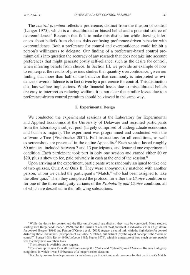
We judged 15 seconds to be enough time to read the question and gauge diffi-culty, but short enough to render solving the questions unlikely.8 Participants were reminded that, when it was time to answer the questions, they would have an entire minute to do so. The questions were previewed in the order they appeared on the quizzes, with the exception that the source alternated between the quiz the participant was to take and the Match’s quiz. Figure 1 shows a screenshot of a sample preview screen. Participants were told that they would answer each question in Part 3, but they did not learn about the asset choices of Part 2 until after Part 1 was completed.

After 15 seconds, the screen automatically advanced to a belief-elicitation screen. If the previewed question had been from the participant’s own quiz, she entered the percent chance with which she believed she would answer that question correctly. We denote the corresponding probability p s . Figure 2 shows a screenshot of the elicitation.

For questions from the Match’s quiz, the participant entered the percent chance with which she believed her Match would answer the question correctly, with the probability denoted p m . We varied the information provided on this screen across three ambiguity variants of the PC condition. In the Probability and Choice: Baseline (PCB) condition, the only information participants had to inform p m was the ques-tion itself. In the Probability and Choice: reduced Ambiguity (PCRA) condition, the participant was also given her Match’s own stated p s , p s (M ), an indicator of the

8 A longer preview period may have led to extreme estimates for each participant’s own questions, reducing the likelihood that the asset choices would feature similar likelihoods.

Vol. 6 No. 4 143owens et al.: the control premium

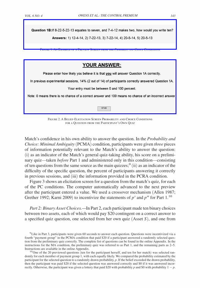
Match’s confidence in his own ability to answer the question. In the Probability and Choice: Minimal Ambiguity (PCMA) condition, participants were given three pieces of information potentially relevant to the Match’s ability to answer the question: (i) as an indicator of the Match’s general quiz-taking ability, his score on a prelimi-nary quiz—taken before Part 1 and administered only in this condition—consisting of ten questions from the same source as the main quizzes;9 (ii) as an indicator of the difficulty of the specific question, the percent of participants answering it correctly in previous sessions, and (iii) the information provided in the PCRA condition.

Figure 3 shows an elicitation screen for a question from the match’s quiz, for each of the PC conditions. The computer automatically advanced to the next preview after the participant entered a value. We used a crossover mechanism (Allen 1987; Grether 1992; Karni 2009) to incentivize the statements of p s and p m for Part 1.10

Part 2: Binary Asset Choices.—In Part 2, each participant made ten binary choices between two assets, each of which would pay $20 contingent on a correct answer to a specified quiz question, one selected from her own quiz (Asset S ), and one from

9 Like in Part 3, participants were given 60 seconds to answer each question. Questions were incentivized via a fourth “payment group” in the PCMA condition that paid $20 if a participant answered a randomly selected ques-tion from the preliminary quiz correctly. The complete list of questions can be found in the online Appendix. In the instructions for the MA condition, the preliminary quiz was referred to as Part 1, and the remaining parts as 2–5. Instructions are available in the online Appendix.

10 One of the 20 previewed questions (ten for the participant herself, and ten for her match) was selected ran-domly for each member of payment group 1, with each equally likely. We compared the probability estimated by the participant for the selected question to a randomly drawn probability, p. If the belief exceeded the drawn probability, then the participant was paid $20 if the selected question was answered correctly and $0 if it was answered incor-rectly. Otherwise, the participant was given a lottery that paid $20 with probability p and $0 with probability 1 − p.

Figure 1. An Example of a Preview Screen from the Probability and ChoiCe Conditions

Figure 2. A Belief-Elicitation Screen Probability and Choice Conditions for a Question from the Participant’s Own Quiz

144 AMeriCAN eCoNoMiC JourNAl: MiCroeCoNoMiCS NoVeMBer 2014

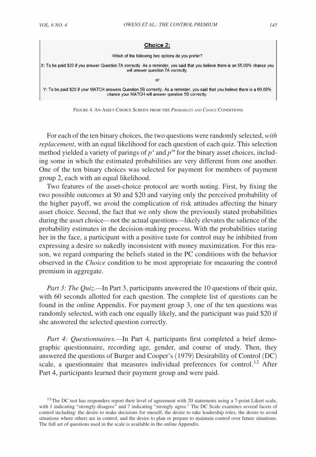
her Match’s (Asset M ) quiz.11 Only after completing Part 1 did participants read the instructions to Part 2. Thus, they expressed p s and p m in Part 1 without the knowl-edge that the binary asset choices in Part 2 were to come. As shown in Figure 4, each participant was reminded of the probabilities, p s and p m , that she herself had previously estimated for each corresponding correct answer. Participants were not shown the questions themselves at this point, as this would allow them to reassess the likelihood of correct answers, possibly rendering the previously stated p s and p m inaccurate. Importantly, p s and p m were the only pieces of information that partici-pants had on which to base their choice of assets.

11 During the experiment sessions, the neutral terms “Option X” and “Option Y” were used to refer to “Asset S” and “Asset M,” respectively, as shown in Figure 4.

Panel A. Baseline

Panel B. Reduced ambiguity

Panel C. Minimal ambiguity

Figure 3. Belief Elicitation Screen from the Probability and ChoiCe Conditions for a Question from the Match’s Quiz

Vol. 6 No. 4 145owens et al.: the control premium

For each of the ten binary choices, the two questions were randomly selected, with replacement, with an equal likelihood for each question of each quiz. This selection method yielded a variety of parings of p s and p m for the binary asset choices, includ-ing some in which the estimated probabilities are very different from one another. One of the ten binary choices was selected for payment for members of payment group 2, each with an equal likelihood.

Two features of the asset-choice protocol are worth noting. First, by fixing the two possible outcomes at $0 and $20 and varying only the perceived probability of the higher payoff, we avoid the complication of risk attitudes affecting the binary asset choice. Second, the fact that we only show the previously stated probabilities during the asset choice—not the actual questions—likely elevates the salience of the probability estimates in the decision-making process. With the probabilities staring her in the face, a participant with a positive taste for control may be inhibited from expressing a desire so nakedly inconsistent with money maximization. For this rea-son, we regard comparing the beliefs stated in the PC conditions with the behavior observed in the Choice condition to be most appropriate for measuring the control premium in aggregate.

Part 3: The Quiz.—In Part 3, participants answered the 10 questions of their quiz, with 60 seconds allotted for each question. The complete list of questions can be found in the online Appendix. For payment group 3, one of the ten questions was randomly selected, with each one equally likely, and the participant was paid $20 if she answered the selected question correctly.

Part 4: Questionnaires.—In Part 4, participants first completed a brief demo-graphic questionnaire, recording age, gender, and course of study. Then, they answered the questions of Burger and Cooper’s (1979) Desirability of Control (DC) scale, a questionnaire that measures individual preferences for control.12 After Part 4, participants learned their payment group and were paid.

12 The DC test has responders report their level of agreement with 20 statements using a 7-point Likert scale, with 1 indicating “strongly disagree” and 7 indicating “strongly agree.” The DC Scale examines several facets of control including: the desire to make decisions for oneself, the desire to take leadership roles, the desire to avoid situations where others are in control, and the desire to plan or prepare to maintain control over future situations. The full set of questions used in the scale is available in the online Appendix.

Figure 4. An Asset-Choice Screen from the Probability and ChoiCe Conditions

146 AMEriCAN ECoNoMiC JourNAL: MiCroECoNoMiCs NoVEMBEr 2014

B. The Choice Condition

Participants in the Choice (C) condition simply chose between Assets s and M, but were never asked to report estimates of p s or p m . Instead, they were simply shown the question previews and asked to choose, as shown in Figure 5. They were allowed 30 seconds to make their asset choice, matching the combined preview time in the PC conditions. The 22 participants in this condition each answered 15 ques-tions and made 15 binary choices, compared to 10 each in the PC conditions. Other aspects of the Choice condition, including payment13 and the questionnaire, mimic those in the PC conditions.

II. Results

We conducted 11 sessions with a total of 108 participants (22 in C, 33 in PCB, 27 in PCRA, and 26 in PCMA), yielding a total of 330 answers and choices in the C condition and 860 answers and 860 choices in the three PC conditions. We discarded 14 asset choices in the C condition and 47 in the PC conditions, for which we lacked probability estimates or for which choices were not entered in time, leaving 316 choices for our analysis in the C condition, and 813 in the PC conditions.14 The cho-sen asset paid off in 454 (40.2 percent) of the 1,129 decisions, yielding an expected earnings from the asset choice of $8.04—worse than if participants had chosen ran-domly. Average total earnings across all sessions were approximately $17.

We begin with aggregate analysis, comparing between-subjects the choices in the C condition with the probability estimates in the PC conditions, treating each choice as an independent observation and ignoring individual effects. Having both

13 There were only two payment groups in the Choice condition, analogous to payment groups 2 and 3 in the PC conditions.

14 For the first 6 sessions, the program recorded a default likelihood of 0 if no likelihood was entered, so subjects were unable to distinguish whether their Match failed to make an estimate in time, or they actively entered a prob-ability of 0. Thus, for these sessions, all binary choices for which p s = 0 or p m = 0 are omitted from our analysis.

Question 14B: Tom is younger than Rose, but older than Will and Jack, in that order. Rose is younger than Susie, but older than Jack.

Jack is younger than Jim. Susie is older than Rose, but younger than Jim. Jim is older than Tom. Who is the oldest?

Answers: 1) Rose, 2) Will, 3) Jack, 4) Jim, or 5) Susie

Question 11A: At my favorite fruit stand in Puzzleland, an orange costs18 cents, a pineapple costs 27 cents, and a grape costs 15 cents.

Using the same logic, how much does a mango cost?

Answers: 1) 7 cents, 2) 11 cents, 3) 15 cents, 4) 18 cents, or 5) 24 cents

Option X pays you $20.00 if youanswer your Question Correctly.

Option Y pays you $20.00 if yourMATCH answers their question

correctly.

Do you prefer Option X or Option Y?

Choice 1:

Your Question:

Your Match’s Question:

Figure 5. An Asset-Choice Screen from the ChoiCe Condition

VoL. 6 No. 4 147owens et al.: the control premium

choice and belief data from participants in the PC conditions, we also compare their beliefs to their own choices in the aggregate. We then turn to individual behavior, examining the consistency of beliefs and choices within-subject in the PC condi-tions. Finally, we compare behavior across the three PC conditions to assess the sensitivity of our results to the presence of ambiguity. In the Appendix, we provide further analysis of the accuracy and formation of beliefs and of the findings of the post-quiz questionnaire.

A. Aggregate Analysis

Participants in the Choice condition heavily favor Asset s. Figure 6 summarizes the number of times out of her 15 asset choices that each individual participant chose Asset s.15 Eighteen out of 22 participants choose Asset s in more than half of their opportunities. In the aggregate, participants’ widespread tendency toward self-reliance is shown in the top row of Table 1, which reports that in their 316 asset choices, these participants selected Asset s 205 times (64.9 percent).

Next, we examine the extent to which this tendency is consistent with choosing the asset perceived most likely to yield the $20 payment, a behavior that maximizes expected earnings and we refer to as following the p-max strategy. The last column of Table 1 reports the rate at which, given the beliefs reported by participants in the PC conditions, Asset s would be chosen under the p-max strategy, calculated as the proportion of choices for which p s > p m , plus exactly half of the instances for

15 Of the 330 total binary choices, 14 from 8 different participants were not entered within the allotted 30 sec-onds. For these participants, we normalized by multiplying the percentage of their entered choices favoring Asset s by 15.

0

1

2

3

4

5

Fre

quen

cy

0 1 2 3 4 5 6 7 8 9 10 11 12 13 14 15

Figure 6. A Histogram of the Frequency with Which Individual Participants Chose Asset S in the ChoiCe Condition

148 AMEriCAN ECoNoMiC JourNAL: MiCroECoNoMiCs NoVEMBEr 2014

which p s = p m . In this counterfactual, Asset s is favored in only 56.4 percent of the 813 choices, which is a lower proportion than that observed in the C condition.16 Thus, the Choice condition participants chose Asset s at a rate 15 percent in excess of that predicted. The 8.5 percentage point gap between the two conditions reflects a residual preference for some property of Asset s, such as payoff autonomy or self-reliance, which is independent of the asset’s perceived financial properties and cannot be explained by miscalibrated beliefs. We use the control premium as an umbrella label to refer to the willingness-to-pay for this property.

In the Probability and Choice conditions, participants first estimate p s and p m and then are confronted with these estimations when they make their asset choices. We hypothesize that this process would inhibit the expression of the control pre-mium and, indeed, behavior in these conditions hews closer to the p-max strategy. Participants chose Asset s in 59.9 percent of their choices, less frequently than the 64.9 percent in the C condition.

Because the control premium is more likely to impact behavior when the differ-ences in expected earnings are small, we now focus on the subset of the choices in the PC conditions for which p s and p m are within 0.10 of each other. The bottom row of Table 1 shows, for this subset, the p-max prediction for Asset s choices and the actual choices. Despite a lower p-max prediction of 53.8 percent, the 65.8 percent rate at which Asset s was chosen is higher than that of the overall sample. This “close calls” subset constitutes 29 percent of the overall sample, but accounts for 66 percent of the deviations from the p-max strategy. Thus, the control premium mainly affects choices for which the difference in expected returns for the two assets is small, but it plays a major role in these choices. In other words, participants are sensitive to the cost of con-trol, as if the premium they are willing to pay for control is stable and well-behaved.

This price sensitivity is further illustrated in Figure 7, which charts the frequency with which Asset s was chosen for various levels of p s − p m in the PC conditions. When | p s − p m | > 0.20, subjects almost exclusively conformed to the p-max strat-egy. We see low levels of deviation when 0.10 < | p s − p m | ≤ 0.20 and even more when 0 < | p s − p m | ≤ 0.10, in both cases with greater deviation to the left of 0,

16 For 67 of the 813 observations in the PC conditions, p s = p m , meaning that an expected money maximizer would be indifferent between the two assets. For the purposes of constructing a counterfactual behavioral bench-mark, we choose to assume that an expected money maximizer would randomize between the assets in these cases and be equally likely to choose each asset. Though we could use other methods to calculate the benchmark, this method feels the most evenhanded and, among other possible methods, even the least charitable yields the same qualitative conclusion. The p-max benchmark becomes 56.9 percent (426 of 749) if choices for which p s = p m are excluded.

Table 1—Percent of Choices for Which Asset S was Actually Chosen and the Percent Predicted under the p-max Strategy Given Reported Beliefs

Observations s chosen p-max

Choice 316 64.9 —Probability and choice 813 59.9 56.4Probability and choice, | p s − p m | ≤ 0.10 234 65.8 53.8

VoL. 6 No. 4 149owens et al.: the control premium

where deviating comes in the form of favoring Asset s at a cost. Importantly, choices at p s − p m = 0 heavily favored Asset s.

B. individual Analysis

As participants in the PC conditions repeatedly chose between assets about which they have expressed their beliefs, we can analyze the consistency of their choices across the session. First, we examine the frequency with which each indi-vidual participant chose to sacrifice expected earnings to retain or avoid control. Then we analyze the extent to which each individual’s behavior was consistent with a well-behaved decision rule that trades off expected returns for control, and make comparisons across such participants.

The histograms in Figure 8 show the frequency with which participants in the PC conditions opted for Asset s, with the results for the C condition alongside for

0

0.1

0.2

0.3

0.4

0.5

0.6

0.7

0.8

0.9

1

Cho

ice

of A

sset

S

<−0.5<−0.4<−0.3<−0.2<−0.1 <0 =0 >0 >0.1 >0.2 >0.3 >0.4 >0.5

Figure 7. The Rate at Which Asset S is Chosen in the PC Conditions, by ( p s − p m )

Figure 8. Histogram of the Percentage of Instances in Which Participants Chose Asset S

Fra

ctio

n

0 10 20 30 40 50 60 70 80 90 100

Panel A. C condition

0

0.1

0.2

0.3

0.4

0.5

0

0.1

0.2

0.3

0.4

0.5

Fra

ctio

n

0 10 20 30 40 50 60 70 80 90 100

Panel B. PC conditions

150 AMEriCAN ECoNoMiC JourNAL: MiCroECoNoMiCs NoVEMBEr 2014

comparison.17 Eighty-four participants from the PC conditions are represented.18 There is more variance in the selection of Asset s in the PC conditions, principally driven by the varying levels of confidence expressed. With the exception of 1 par-ticipant, who chose asset s all 10 times, all participants in the PC conditions chose both assets at least once, with a large majority doing so in 40 percent to 80 percent of the decisions.19

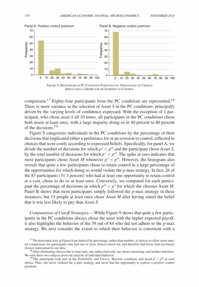
Figure 9 categorizes individuals in the PC conditions by the percentage of their decisions that implicated either a preference for or an aversion to control, reflected in choices that were costly according to expressed beliefs. Specifically, for panel A, we divide the number of decisions for which p s < p m and the participant chose Asset s, by the total number of decisions for which p s < p m . The spike at zero indicates that most participants chose Asset M whenever p s < p m . However, the histogram also reveals that quite a few participants chose to retain control in a large percentage of the opportunities for which doing so would violate the p-max strategy. In fact, 26 of the 83 participants (31.3 percent) who had at least one opportunity to retain control at a cost, chose to do so at least once. Conversely, we computed for each partici-pant the percentage of decisions in which p m < p s for which she chooses Asset M. Panel B shows that most participants simply followed the p-max strategy in these instances, but 15 people at least once chose Asset M after having stated the belief that it was less likely to pay than Asset s.

Computation of Cutoff strategies.—While Figure 9 shows that quite a few partic-ipants in the PC conditions always chose the asset with the higher expected payoff, it also highlights the behavior of the 39 out of 84 who did not adhere to the p-max strategy. We next consider the extent to which their behavior is consistent with a

17 The horizontal axes in Figure 8 are indexed by percentage, rather than number, of choices to allow more natu-ral comparisons for participants who had one or more choices timed out, and therefore had fewer than ten binary choices represented in our data.

18 After eliminating choices due to time-outs, one subject had only one choice remaining, and another had three. We omit these two subjects from our analysis of individual behavior.

19 This participant took part in the Probability and Choice: Baseline condition, and faced p s > p m in each choice. Thus, she never violated the p-max strategy, and never had the opportunity to express a positive control premium.

0

10

20

30

40

50

60

70

0

10

20

30

40

50

60

70

Fre

quen

cy

0 10 20 30 40 50 60 70 80 90 100

Panel A. Positive control premium

Fre

quen

cy

0 10 20 30 40 50 60 70 80 90 100

Panel B. Negative control premium

Figure 9. Histograms of PC Condition Participants’ Percentage of Choices Implicating a Desire for or Aversion to Control

VoL. 6 No. 4 151owens et al.: the control premium

price-sensitive decision rule. We begin by noting that as the difference ( p s − p m ) increases, Asset s becomes relatively more attractive. If participants trade off a valuation for control, whether positive, zero, or negative, for expected earnings, their choices will be consistent with a cutoff strategy in ( p s − p m ), favoring Asset s whenever ( p s − p m ) exceeds some cutoff p , and choosing Asset s whenever ( p s − p m ) falls short of p . The p-max strategy corresponds to a cutoff of ( p s − p m ) = 0. However, a person willing to pay a premium to retain or avoid payoff autonomy would employ a nonzero cutoff, with p < 0 corresponding to a positive premium on control and p > 0 corresponding to a negative control premium.

A participant’s behavior is consistent with a cutoff strategy if the minimum value of ( p s − p m ) for which she chose Asset s, which we denote p s _ , is no less than the maximum value of ( p s − p m ) for which she chose Asset M, denoted

_ p m . Sixty-nine

of the 84 (82 percent) participants in the PC conditions behaved in a manner con-sistent with a cutoff strategy. Of the 39 participants who did not adhere strictly to the p-max strategy, the behavior of 24 (62 percent) was still consistent with a cutoff. Thus, many deviations from the p-max strategy are consistent with a willingness to pay for control, not merely noise or trembling.

We do not observe cutoffs directly, so we impute them for the 69 participants in the PC conditions with cutoff-consistent behavior. Because the cutoff is bounded by _ p m and p s _ , we begin by applying a simple “midpoint rule” that assigns the cutoff

to be p = ( _ p m + p s _ )/2.20 Figure 10, panel A displays the distribution of cutoffs

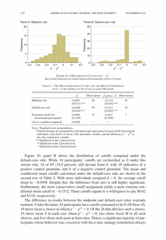
calculated according to this rule. While the distribution is peaked at 0, it is clearly skewed to the left, and the cutoffs range from −0.475 to 0.275 in value. Forty-five participants exhibit a positive control premium, 10 have a cutoff of 0, and 13 have a negative control premium, when cutoffs are calculated in this way.

The top row of Table 2 displays the mean cutoff and the mean conditional on displaying a positive control premium ( p < 0), calculated using the midpoint rule. The mean cutoff of −0.0597 is significantly less than 0, equivalent to a willingness to relinquish $1.19 of expected return to retain payoff autonomy. Among the 45 individuals exhibiting a positive control premium, the average cutoff is −0.1119, corresponding to a premium of $2.24 on control.

While illustrative, the midpoint rule has the drawback of assigning a nonzero cutoff to some participants who never expressly violated the p-max strategy.21 A more conservative approach is to assign a default cutoff of p = 0 to all participants who never violate the p-max strategy, and to use the midpoint rule for those who are consistent with a cutoff in p s − p m but deviate from the p-max strategy at some point. This “default-zero” rule reassigns a 0 cutoff to 27 participants classified as having a positive control premium under the midpoint rule and does so to 7 classi-fied as having a negative control premium.22

20 Using this method to compute the cutoff, we exclude the one participant who had p s > p m in every choice and thus, for whom

_ p m is undefined.

21 For example, the rule estimates the cutoff of a participant for whom _ p m = −0.20 and p s _ = 0 as

( p m _ + _ p s )/2 = −0.10, though her choices are consistent with a cutoff of zero.

22 This rule also assigns a zero cutoff to the participant who chose Asset s in each choice.

152 AMEriCAN ECoNoMiC JourNAL: MiCroECoNoMiCs NoVEMBEr 2014

Figure 10, panel B shows the distribution of cutoffs computed under the default-zero rule. While 34 participants’ cutoffs are reclassified as 0 under this stricter rule, 24 of 69 (34.8 percent) still deviate from 0, with 18 indicative of a positive control premium, and 6 of a negative control premium. The mean and conditional mean cutoffs calculated under the default-zero rule are shown in the second row of Table 2. With more individuals assigned p = 0, the average cutoff drops to −0.0308. Despite this, the difference from zero is still highly significant. Furthermore, the more conservative cutoff assignment yields a more extreme con-ditional mean cutoff of −0.1512. These cutoffs equate to a willingness to pay $0.62 and $3.02, respectively.

The difference in results between the midpoint and default-zero rules warrants mention. Under the latter, 45 participants have cutoffs estimated to be 0. Of these 45, 19 never faced a choice in which p s − p m = 0. Of the 26 that did face such a choice, 19 chose Asset s in each case where p s − p m = 0, two chose Asset M in all such choices, and five chose each asset at least once. Hence, a significant majority of par-ticipants whose behavior was consistent with the p-max strategy nonetheless always

0

5

10

15

20

Fre

quen

cy

−0.4 −0.3 −0.2 −0.1 0 0.1 0.2 −0.4 −0.3 −0.2 −0.1 0 0.1 0.2

Panel A. Midpoint rule

0

10

20

30

40

50

Fre

quen

cy

Panel B. Default-zero rule

ps − pm ps − pm

Figure 10. A Histogram of Cutoffs in p s − p m . Excludes Participants with Choices Inconsistent with a Cutoff

Table 2—The Mean Individual Cutoff and the Mean Conditional on p < 0 According to Two Calculation Methods

_ p Observations

_ p given < 0 Observations

Midpoint rule −0.0597 68 −0.1119 45(0.0131)*** (0.0136)***

Default zero rule −0.0308 69 −0.1512 18(0.0110)*** (0.0222)***

Estimated cutoffs for −0.0505 15 −0.2471 7 inconsistent participantsa (0.1540) (0.1509)Choice condition [imputed] −0.0700 — —

Notes: Standard errors in parentheses.a Cutoff estimates are generated by individual logit regressions for each cutoff-inconsistent individual, with choice of Asset s the dependent variable, and the difference p s − p m as the only explanatory variable.

*** Significant at the 1 percent level. ** Significant at the 5 percent level. * Significant at the 10 percent level.

VoL. 6 No. 4 153owens et al.: the control premium

choose Asset s in the case of ties. This residual “weak” preference for Asset s explains the magnitude of the difference in p between the two estimation methods.

Analysis of Cutoff-inconsistent Participants.—The 15 participants whose choices are not consistent with a cutoff strategy represent 18 percent of the overall sample. To what extent does their exclusion from the individual analysis affect the conclu-sions that we draw from it? We answer this question by estimating a cutoff for each of these individuals using a logit regression. The dependent variable is an indicator for having chosen Asset s, and the difference p s − p m is the only independent vari-able. The cutoff estimate is the ratio of the coefficient on p s − p m to the constant term. Intuitively, this is the value of p s − p m for which the the probability of choos-ing Asset s changes from 0 to 1.

The mean of these cutoff estimates, reported in the third row of Table 2, is −0.0505. This implies indifference between the 2 assets when M is 5 percentage points more likely to pay off and is nearly identical to the mean calculated under the midpoint rule. Unsurprisingly, the mean of these estimates is significantly dif-ferent from neither the mean cutoff calculated under the midpoint rule ( p = 0.90 according to a two-tailed Welch’s t-test) nor the mean calculated under default-zero rule ( p = 0.79). Definitive conclusions cannot be drawn from this small subsample, but these estimates do not suggest preferences that are dramatically different from those who follow a cutoff strategy. Thus, there is little evidence that our conclu-sions from the individual analysis are significantly affected by the exclusion of the cutoff-inconsistent participants.

How do these 15 participants color our understanding of aggregate behavior? In Section IIA, we paid particular attention to the subset of observations for which the difference in expected earnings between the two assets is small. However, out of the 579 observations for which the differences in expected earnings is more extreme (| p s − p m | > 0.10), there still are a number of deviations from the p-max strategy. All 11 such deviations that were consistent with a negative control premium are attribut-able to cutoff-inconsistent individuals. In contrast, 8 out of 12 extreme deviations that were consistent with a positive control premium came from cutoff-consistent individuals. Furthermore, these 8 deviations were more moderate, with | p s − p m | values ranging from 0.11 to 0.25 and having a mean of 0.18, while, in contrast, the 4 observations that were from cutoff-inconsistent individuals had a mean of 0.33. Thus, the observations that are the least consistent with the picture painted by our main aggregate analysis, that of a moderate, stable, and well-behaved preference for control, are generated by the same individuals whose noisy or trembling behavior poses the greatest challenge for our individual analysis.

Aggregate Cutoff in the Choice Condition.—As participants in the Choice condi-tion did not express p s and p m , we can neither calculate cutoffs nor characterize the control premium at the individual level. However, we can make a between-subjects comparison of the choices from the C condition and beliefs from the PC conditions to impute an aggregate cutoff for participants in the C condition. Roughly 65 per-cent of choices in the C condition favor Asset s. Thus, the thirty-fifth percentile of p s − p m in the PC conditions is a reasonable estimate for the average value of

154 AMEriCAN ECoNoMiC JourNAL: MiCroECoNoMiCs NoVEMBEr 2014

p s − p m for which participants in the C condition are indifferent between Assets s and M. This cutoff value, −0.0700, reflects a stronger aggregate preference for control than we calculated from the PC conditions, using both the midpoint and default-zero rules. Thus, both the aggregate analysis and the individual cutoff cal-culations support our claim that the salience of the expressed probabilities in the PC conditions dampens the expression of the control premium.

C. Comparisons across Conditions: The Effect of reducing Ambiguity

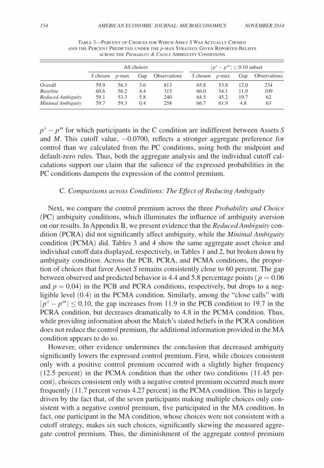
Next, we compare the control premium across the three Probability and Choice (PC) ambiguity conditions, which illuminates the influence of ambiguity aversion on our results. In Appendix B, we present evidence that the reduced Ambiguity con-dition (PCRA) did not significantly affect ambiguity, while the Minimal Ambiguity condition (PCMA) did. Tables 3 and 4 show the same aggregate asset choice and individual cutoff data displayed, respectively, in Tables 1 and 2, but broken down by ambiguity condition. Across the PCB, PCRA, and PCMA conditions, the propor-tion of choices that favor Asset s remains consistently close to 60 percent. The gap between observed and predicted behavior is 4.4 and 5.8 percentage points ( p = 0.06 and p = 0.04) in the PCB and PCRA conditions, respectively, but drops to a neg-ligible level (0.4) in the PCMA condition. Similarly, among the “close calls” with | p s − p m | ≤ 0.10, the gap increases from 11.9 in the PCB condition to 19.7 in the PCRA condition, but decreases dramatically to 4.8 in the PCMA condition. Thus, while providing information about the Match’s stated beliefs in the PCRA condition does not reduce the control premium, the additional information provided in the MA condition appears to do so.

However, other evidence undermines the conclusion that decreased ambiguity significantly lowers the expressed control premium. First, while choices consistent only with a positive control premium occurred with a slightly higher frequency (12.5 percent) in the PCMA condition than the other two conditions (11.45 per-cent), choices consistent only with a negative control premium occurred much more frequently (11.7 percent versus 4.27 percent) in the PCMA condition. This is largely driven by the fact that, of the seven participants making multiple choices only con-sistent with a negative control premium, five participated in the MA condition. In fact, one participant in the MA condition, whose choices were not consistent with a cutoff strategy, makes six such choices, significantly skewing the measured aggre-gate control premium. Thus, the diminishment of the aggregate control premium

Table 3—Percent of Choices for Which Asset S Was Actually Chosen and the Percent Predicted under the p-max Strategy Given Reported Beliefs

across the Probability & ChoiCe Ambiguity Conditions

All choices | p s − p m | ≤ 0.10 subset

s chosen p-max Gap Observations s chosen p-max Gap Observations

Overall 59.9 56.3 3.6 813 65.8 53.8 12.0 234Baseline 60.6 56.2 4.4 315 66.0 54.1 11.9 109reduced Ambiguity 59.1 53.3 5.8 240 64.5 45.2 19.7 62Minimal Ambiguity 59.7 59.3 0.4 258 66.7 61.9 4.8 63

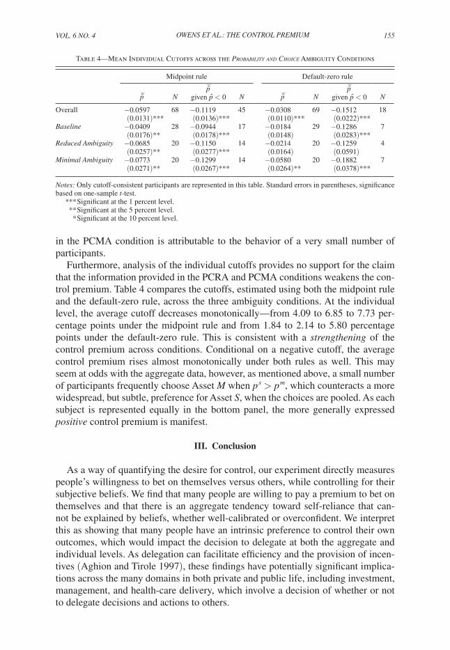
VoL. 6 No. 4 155owens et al.: the control premium

in the PCMA condition is attributable to the behavior of a very small number of participants.

Furthermore, analysis of the individual cutoffs provides no support for the claim that the information provided in the PCRA and PCMA conditions weakens the con-trol premium. Table 4 compares the cutoffs, estimated using both the midpoint rule and the default-zero rule, across the three ambiguity conditions. At the individual level, the average cutoff decreases monotonically—from 4.09 to 6.85 to 7.73 per-centage points under the midpoint rule and from 1.84 to 2.14 to 5.80 percentage points under the default-zero rule. This is consistent with a strengthening of the control premium across conditions. Conditional on a negative cutoff, the average control premium rises almost monotonically under both rules as well. This may seem at odds with the aggregate data, however, as mentioned above, a small number of participants frequently choose Asset M when p s > p m , which counteracts a more widespread, but subtle, preference for Asset s, when the choices are pooled. As each subject is represented equally in the bottom panel, the more generally expressed positive control premium is manifest.

III. Conclusion

As a way of quantifying the desire for control, our experiment directly measures people’s willingness to bet on themselves versus others, while controlling for their subjective beliefs. We find that many people are willing to pay a premium to bet on themselves and that there is an aggregate tendency toward self-reliance that can-not be explained by beliefs, whether well-calibrated or overconfident. We interpret this as showing that many people have an intrinsic preference to control their own outcomes, which would impact the decision to delegate at both the aggregate and individual levels. As delegation can facilitate efficiency and the provision of incen-tives (Aghion and Tirole 1997), these findings have potentially significant implica-tions across the many domains in both private and public life, including investment, management, and health-care delivery, which involve a decision of whether or not to delegate decisions and actions to others.

Table 4—Mean Individual Cutoffs across the Probability and ChoiCe Ambiguity Conditions

Midpoint rule Default-zero rule

_ p N

_ p

given p < 0 N _ p N

_ p

given p < 0 N

Overall −0.0597 68 −0.1119 45 −0.0308 69 −0.1512 18(0.0131)*** (0.0136)*** (0.0110)*** (0.0222)***

Baseline −0.0409 28 −0.0944 17 −0.0184 29 −0.1286 7(0.0176)** (0.0178)*** (0.0148) (0.0283)***

reduced Ambiguity −0.0685 20 −0.1150 14 −0.0214 20 −0.1259 4(0.0257)** (0.0277)*** (0.0164) (0.0591)

Minimal Ambiguity −0.0773 20 −0.1299 14 −0.0580 20 −0.1882 7(0.0271)** (0.0267)*** (0.0264)** (0.0378)***

Notes: Only cutoff-consistent participants are represented in this table. Standard errors in parentheses, significance based on one-sample t-test.

*** Significant at the 1 percent level. ** Significant at the 5 percent level. * Significant at the 10 percent level.

156 AMEriCAN ECoNoMiC JourNAL: MiCroECoNoMiCs NoVEMBEr 2014

What is the precise motivation that drives our findings? One factor that we explicitly consider is ambiguity aversion. Across our three PC conditions, we find mixed results as to whether reducing the differences in ambiguity between Asset s and Asset M reduce the control premium. Because we find no decrease in average individual cutoffs, the more direct and reliable measure of the control premium, as ambiguity decreases, we conclude that the desire for control does exert a signifi-cant influence on the choices of many individuals, independent of attitudes toward ambiguity.

However, the control premium is an umbrella term that is consistent with more than one specific motivation and there remains room for interpretation as to what underlies our participants’ preference to bet on themselves. While people may place a premium on payoff autonomy in any context, it is possible that our results were influenced by the betting aspect of our methodology, as it may be more enjoyable to bet on oneself than to bet on someone else. People may like to bet on themselves in the same way they like to bet on (and not against) sports teams that they support. While our research clearly has direct implications for our understanding of delega-tion decisions in risky environments, more research is necessary to unpack further the motivation driving our results and thus clarify the full range of contexts to which it is most relevant.

The manner in which we incentivize beliefs presents a reason why our method of measuring the desire for control may understate its impact in the field. We use a crossover or lottery mechanism (Allen 1987; Grether 1992; Karni 2009) to elicit probabilities, which avoids bias due to risk attitudes, but introduces a possible bias that would lower the measured value of the control premium. While we focus on an individual’s desire to control her own outcomes instead of ceding that control to another person, she may also prefer control of her own outcomes to ceding control to a random process. Such a “self-random” control premium would bias upward the stated beliefs about one’s own performance that we elicit and therefore bias downward our estimate of the “self-other” control premium.23 For this reason, our measure should be viewed as providing a lower bound on the control premium’s influence on decisions in the field.

We observe a symmetric distribution of quiz scores (see A.A1), which is consis-tent with a symmetric distribution of quiz-taking abilities. Given such symmetry, the fact that each quiz question is equally likely to appear in our data as either Asset s or Asset M, means that a population of expected-money maximizers with correct beliefs would be expected to choose Asset s in exactly 50 percent of all observations. Using this benchmark, we identify the 64.9 percent rate at which Asset s was chosen in the Choice condition as representing a 14.9 percentage point excess of self-reliance, of which 6.4 percentage points (43 percent)—the gap between 50.0 percent and the p-max prediction of 56.4 percent—are due to overconfident beliefs and the remain-ing 8.5 percentage points (57 percent) are due to the control premium.

This decomposition allows to highlight the potential pitfalls of relying unhesitat-ingly on choice data to characterize beliefs. We do this by reinterpreting the results

23 If the “other-random” control premium is larger than the “self-random” control premium, then our results overstate the “self-other” control premium. We find this unlikely.

VoL. 6 No. 4 157owens et al.: the control premium

of Hoelzl and Rustichini (2005), who had each participant in their experiment com-plete a test, then vote either to have her payment determined by whether or not she scored above the median or to have it determined by the outcome of a 50–50 lottery. Participants in their Easy, Money condition voted for the test-based payment 63 per-cent, rather than 50 percent, of the time, which the authors interpret as evidence of overconfidence in the population.24 However, if, like in our experiment, 57 percent of the excess self-reliance cannot be attributed to beliefs, then a more appropriate interpretation of their result is that overconfidence explains 5.5 percentage points of deviation from 50 percent, while 7.5 percentage points can only be explained by a desire for control. Thus, careful attention to the influence of preferences ver-sus beliefs in generating self-reliance can yield more sound behavioral and welfare interpretations of experimental results.

Appendix: Supplemental Results

A. Quiz results

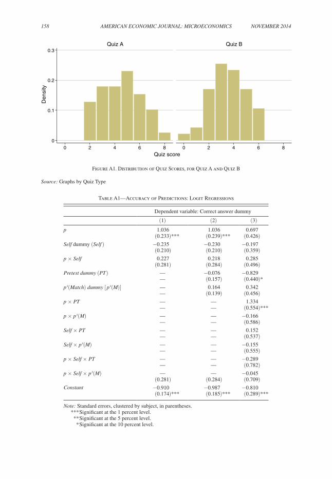
The 86 participants in the Probability and Choice conditions answered an average of 4.00 out of 10 questions correctly. Those taking Quiz A did better, answering an average of 4.51 (s.e. 0.26) correctly, while those taking Quiz B answered 3.57 (0.21) accurately. Figure A1 shows the distribution of the scores for Quiz A and Quiz B, both of which are single-peaked, and appear relatively symmetric. Medians of 5 for Quiz A and 4 for Quiz B are close to the respective means, and joint skewness-kurtosis tests fail to reject the null hypotheses that both quiz scores are normally distributed ( p = 0.316 and 0.800, respectively).

B. Ambiguity Manipulation Check

Table A1 shows logit regressions of whether or not a quiz question was answered correctly on a variety of variables that constitute the information provided to or stated by participants. There is one observation for each probability estimate, p s or p m , so each question is represented twice. The dependent variable is equal to 1 if the target question was answered correctly, and 0 otherwise. self is a dummy vari-able, equal to 1 if the explanatory variable p represents a self-estimated ( p s ), and 0 if it represents the estimate of a participant’s Match ( p m ). The dummy variables p s (M) and PT denote participants’ viewing of their Match’s p s , and pretest scores and population success rates,25 respectively.

An analysis of the regressions presented in Table A1 can yield insight into the ambiguity with which participants regard Assets s and M. Coefficients on the

24 We acknowledge the critique of Benoît and Dubra (2011) and Moore and Healy (2008)—which does apply to Hoelzl and Rustichini (2005)—namely that such evidence is, in fact, consistent with rational beliefs and, moreover, better-than-average data is incapable of showing overconfidence. However, our decomposition can be used to rein-terpret the results of any study that quantifies overconfidence by inferring beliefs directly from behavior, including those using methods acceptable in light of this criticism.

25 As the PCMA condition has both of these information sources, and the other conditions neither, we cannot separate the effects of the two classes of information.

158 AMEriCAN ECoNoMiC JourNAL: MiCroECoNoMiCs NoVEMBEr 2014

0

0.1

0.2

0.3

0 2 4 6 8 0 2 4 6 8

Quiz A Quiz BD

ensi

ty

Quiz score

Figure A1. Distribution of Quiz Scores, for Quiz A and Quiz B

source: Graphs by Quiz Type

Table A1—Accuracy of Predictions: Logit Regressions

Dependent variable: Correct answer dummy

(1) (2) (3)

p 1.036 1.036 0.697(0.233)*** (0.239)*** (0.426)

self dummy (self ) −0.235 −0.230 −0.197(0.210) (0.210) (0.359)

p × self 0.227 0.218 0.285(0.281) (0.284) (0.496)

Pretest dummy (PT ) — −0.076 −0.829— (0.157) (0.440)*

p s (Match) dummy [ p s (M)] — 0.164 0.342— (0.139) (0.456)

p × PT — — 1.334— — (0.554)***

p × p s (M) — — −0.166— — (0.586)

self × PT — — 0.152— — (0.537)

self × p s (M) — — −0.155— — (0.555)

p × self × PT — — −0.289— — (0.782)

p × self × p s (M) — — −0.045(0.281) (0.284) (0.709)

Constant −0.910 −0.987 −0.810(0.174)*** (0.185)*** (0.289)***

Note: Standard errors, clustered by subject, in parentheses.*** Significant at the 1 percent level. ** Significant at the 5 percent level. * Significant at the 10 percent level.

VoL. 6 No. 4 159owens et al.: the control premium

variable p and its interactions show how strongly the probability estimates ( p s and p m ) are related to the outcome of correctly answered questions. The coefficient on p × p s (M) is insignificant, while that in p × PT is large and highly significant. Thus, estimates were far better predictors of correct answers in the PCMA condition, but not in the PCRA condition.

No interaction term involving the self variable is significantly related to cor-rectly answered questions. This suggests that participants predicted their Match’s success just as accurately as they predicted their own, in each condition. We take two observations from these regressions. First, the PCRA condition did not signifi-cantly reduce the ambiguity with which participants regarded Asset M, while the PCMA condition did. Second, participants were no better able to predict their own outcomes than their Match’s in any condition, suggesting little or no difference in actual ambiguity between Assets s and M in any condition. However, we cannot with certainty rule out differences in perceived ambiguity, which could help gener-ate the control premium.

C. Questionnaire results

Table A2 shows a number of descriptive statistics: mean total quiz score; mean overconfidence, measured as the sum of the reported probabilities minus the total score; mean frequency of choosing Asset s; and the mean cutoff, calculated sepa-rately for each of the two rules. These statistics are partitioned according to several

Table A2—Summary Statistics by Demographic Characteristics

Quiz Percent Asset s Midpoint ruleb Default zerob

score Overconfidencea choices cutoff cutoff

Female 3.89(0.20)

2.10(0.27)

60.7 (2.60)

−0.0625(0.0184)

−0.0166(0.0130)

Male 4.14(0.25)

1.87(0.25)

61.7 (2.55)

−0.0416(0.0199)

−0.0296(0.0173)

Age ≤20 3.86(0.26)

1.45(0.22)***

61.2 (2.46)

−0.0723(0.0129)

−0.0402(0.0105)

Age >20 4.08(0.19)*

2.28(0.57)***

61.0 (2.70)

−0.0441(0.0505)

−0.0123(0.0350)

Hi BC 3.67(0.20)**

2.54(0.29)***

59.1 (2.41)

−0.0488(0.0225)

−0.0214(0.0164)

Lo BC 4.37(0.24)**

1.51(0.23)***

63.4 (2.76)

−0.0584(0.0156)

−0.0225(0.0134)

Bus-econ major

4.41(0.27)**

1.54(0.25)**

64.6 (2.45)

−0.0698(0.0206)

−0.0358(0.0174)

Other 3.72(0.18)**

2.32(0.26)**

58.8 (2.66)

−0.0418(0.0179)

−0.0115(0.0126)

Notes: Standard errors in parentheses, significance based on one-sample t-test. a Overconfidence is calculated as ∑ i=1

10 i × p i s − Quizscore. b Only cutoffs for cutoff-consistent participants are included, not those imputed using logit

regressions as in Table 2.*** Significant at the 1 percent level. ** Significant at the 5 percent level. * Significant at the 10 percent level.

160 AMERICAN ECONOMIC JOURNAL: MICROECONOMICS NOVEMBER 2014

demographic and personality traits: gender, age, the score on the Burger-Cooper (BC) desire-for-control scale, and course of study. No measure of behavior dif-fers dramatically by gender. Younger participants, those scoring lower on the Burger-Cooper (BC) (Burger and Cooper 1979) test, and Business and Economics (B&E) majors score higher on their quiz than do their counterparts. The latter two groups are also less overconfident, but this could be largely caused by regression to the mean. B&E majors have more extreme cutoffs than their counterparts from other majors, but this difference does not achieve significance.26

REFERENCES

Abdellaoui, Mohammed, Frank Vossmann, and Martin Weber. 2005. “Choice-Based Elicitation and Decomposition of Decision Weights for Gains and Losses under Uncertainty.” Management Sci-ence 51 (9): 1384–99.

Aghion, Philippe, and Jean Tirole. 1997. “Formal and Real Authority in Organizations.” Journal of Political Economy 105 (1): 1–29.

Allen, Franklin. 1987. “Discovering Personal Probabilities When Utility Functions are Unknown.” Management Science 33 (4): 542–44.

Bartling, Björn, and Urs Fischbacher. 2012. “Shifting the Blame: On Delegation and Responsibility.” Review of Economic Studies 79 (1): 67–87.

Bartling, Björn, Ernst Fehr, and Holger Herz. Forthcoming. “The Intrinsic Value of Decision Rights.” Econometrica.

Benjamin, Daniel J., Ori Heffetz, Miles S. Kimball, and Alex Rees-Jones. 2012. “What Do You Think Would Make You Happier? What Do You Think You Would Choose?” American Economic Review 102 (5): 2083–2110.

Benoît, Jean-Pierre, and Juan Dubra. 2011. “Apparent Overconfidence.” Econometrica 79 (5): 1591–1625.

Blavatskyy, Pavlo. 2009. “Betting on Own Knowledge: Experimental Test of Overconfidence.” Journal of Risk and Uncertainty 38 (1): 39–49.

Burger, Jerry M. 1984. “Desire for Control, Locus of Control, and Proneness to Depression.” Journal of Personality 52 (1): 71–89.

Burger, Jerry M. 1986. “Desire for Control and the Illusion of Control: The Effects of Familiarity and Sequence of Outcomes.” Journal of Research in Personality 20 (1): 66–76.

Burger, Jerry M. 1992. Desire for Control: Personality, Social, and Clinical Perspectives. New York: Plenum Press.

Burger, Jerry M., and Harris M. Cooper. 1979. “The Desirability of Control.” Motivation and Emo-tion 3 (4): 381–93.

Camerer, Colin, and Dan Lovallo. 1999. “Overconfidence and Excess Entry: An Experimental Approach.” American Economic Review 89 (1): 306–18.

Charness, Gary, and Uri Gneezy. 2010. “Portfolio Choice and Risk Attitudes: An Experiment.” Eco-nomic Inquiry 48 (1): 133–46.

Coffman, Lucas C. 2011. “Intermediation Reduces Punishment (and Reward).” American Economic Journal: Microeconomics 3 (4): 77–106.

Eil, David, and Justin M. Rao. 2011. “The Good News-Bad News Effect: Asymmetric Processing of Objective Information about Yourself.” American Economic Journal: Microeconomics 3 (2): 114–38.

Ericson, Keith M. Marzilli. 2011. “Forgetting We Forget: Overconfidence and Memory.” Journal of the European Economic Association 9 (1): 43–60.

Falk, Armin, and Michael Kosfeld. 2006. “The Hidden Costs of Control.” American Economic Review 96 (5): 1611–30.

Fehr, Ernst, Holger Herz, and Tom Wilkening. 2013. “The Lure of Authority: Motivation and Incentive Effects of Power.” American Economic Review 103 (4): 1325–59.

26 The sample size is reduced in Table A2 due to a computer malfunction in one of the treatments from the PCMA condition. All binary choice and quiz data was preserved, but data on demographics was lost, so data for 13 participants is not represented in this table.

VOL. 6 NO. 4 161OWENS ET AL.: THE CONTROL PREMIUM

Fenton-O’Creevy, Mark, Nigel Nicholson, Emma Soane, and Paul Willman. 2003. “Trading on Illu-sions: Unrealistic Perceptions of Control and Trading Performance.” Journal of Occupational and Organizational Psychology 76 (1): 53–68.

Fershtman, Chaim, and Uri Gneezy. 2001. “Strategic Delegation: An Experiment.” RAND Journal of Economics 32 (2): 352–68.

Fischbacher, Urs. 2007. “z-Tree: Zurich Toolbox for Ready-Made Economic Experiments.” Experi-mental Economics 10 (2): 171–78.

Grether, David M. 1992. “Testing Bayes Rule and the Representativeness Heuristic: Some Experimen-tal Evidence.” Journal of Economic Behavior and Organization 17 (1): 31–57.

Grossman, Zachary, and David Owens. 2012. “An Unlucky Feeling: Overconfidence and Noisy Feed-back.” Journal of Economic Behavior & Organization 84 (2): 510–24.

Grosswirth, Marvin, Abbie F. Salny, and Alan Stillson. 1999. Match Wits With Mensa: The Complete Quiz Book (Mensa Genius Quiz). New York: Perseus Books.

Hamman, John R., George Loewenstein, and Roberto A. Weber. 2010. “Self-Interest through Delega-tion: An Additional Rationale for the Principal-Agent Relationship.” American Economic Review 100 (4): 1826–46.

Hao, Li, and Daniel Houser. 2012. “Belief Elicitation in the Presence of Naïve Respondents: An Exper-imental Study.” Journal of Risk and Uncertainty 44 (2): 161–80.

Hoelzl, Erik, and Aldo Rustichini. 2005. “Overconfident: Do You Put Your Money on It?” Economic Journal 115 (503): 305–18.

Hollard, Guillaume, Sébastien Massoni, and Jean-Christophe Vergnaud. 2010. “Subjective Beliefs Formation and Elicitation Rules: Experimental Evidence.” Université Panthéon-Sorbonne (Paris 1), Centre d’Economie de la Sorbonne Documents de travail du Centre d’Economie de la Sorbonne 10088.

Holt, Charles A., and Angela M. Smith. 2009. “An Update on Bayesian Updating.” Journal of Eco-nomic Behavior and Organization 69 (2): 125–34.

Karni, Edi. 2009. “A Mechanism for Eliciting Probabilities.” Econometrica 77 (2): 603–06.Langer, Ellen J. 1975. “The Illusion of Control.” Journal of Personality and Social Psychology 32 (2):

311–28.Lefcourt, Herbert M. 1982. Locus of Control: Current Trends in Theory and Research. 2nd ed. Hills-

dale, NJ: Lawrence Erlbaum Associates, Inc.Malmendier, Ulrike, and Geoffrey Tate. 2005. “CEO Overconfidence and Corporate Investment.”

Journal of Finance 60 (6): 2661–2700.Mobius, Markus Michael, Muriel Niederle, Paul Niehaus, and Tanya S. Rosenblat. 2011. “Manag-

ing Self-Confidence: Theory and Experimental Evidence.” National Bureau of Economic Research Working Paper 17014.

Moore, Don A., and Paul J. Healy. 2008. “The Trouble with Overconfidence.” Psychological Review 115 (2): 502–17.

Oexl, Regine, and Zachary J. Grossman. 2013. “Shifting the Blame to a Powerless Intermediary.” Experimental Economics 16 (3): 306–12.

Offerman, Theo, Joep Sonnemans, Gijs Van De Kuilen, and Peter P. Wakker. 2009. “A Truth Serum for Non-Bayesians: Correcting Proper Scoring Rules for Risk Attitudes.” Review of Economic Stud-ies 76 (4): 1461–89.

Owens, David, Zachary Grossman, and Ryan Fackler. 2014. “The Control Premium: A Preference for Payoff Autonomy: Dataset.” American Economic Journal: Microeconomics. http://dx.doi.org/10.1257/mic.6.4.138.

Phares, Jerry E. 1976. Locus of Control in Personality. Morristown, NJ: General Learning Press.Rotter, Julian B. 1990. “Internal versus External Control of Reinforcement: A Case History of a Vari-

able.” American Psychologist 45 (4): 489–93.Selten, Reinhard. 1998. “Axiomatic Characterization of the Quadratic Scoring Rule.” Experimental

Economics 1 (1): 43–61.Svenson, Ola. 1981. “Are We All Less Risky and More Skillful than Our Fellow Drivers?” Acta Psy-

chologica 47 (2): 143–48.

This article has been cited by:

1. David Danz, Dorothea Kübler, Lydia Mechtenberg, Julia Schmid. 2015. On the Failure ofHindsight-Biased Principals to Delegate Optimally. Management Science 150326104019008.[CrossRef]

2. Silvia Dominguez-Martinez, Randolph Sloof, Ferdinand A. von Siemens. 2014. Monitored byyour friends, not your foes: Strategic ignorance and the delegation of real authority. Games andEconomic Behavior 85, 289-305. [CrossRef]