The Analysis of Repeated Measures Designs: A Review

Repeated Measures Analyses 1

The Analysis of Repeated Measures Designs:

A Review

by

H.J. Keselman

University of Manitoba

James Algina

University of Florida

and

Rhonda K. Kowalchuk

University of Manitoba


Abstract

This paper indicates that repeated measures ANOVA can refer to many different

types of analyses. Specifically, this vague terminology could be referring to the

conventional tests of significance, one of three adjusted degrees of freedom univariate

solutions, two different types of multivariate statistics, or approaches that combine

univariate and multivariate tests. Accordingly, by only reporting probability values and

referring to statistical analyses as repeated measures ANOVA, authors, it is argued, do

not convey to readers the type of analysis that was used nor the validity of the reported

probability value, since each of these approaches has its own strengths and weaknesses.

The various approaches are presented with a discussion of their strengths and weaknesses

and recommendations are made regarding the “best” choice of analysis.


The Analysis of Repeated Measures Designs:

A Review

New data analysis strategies that were introduced in the technical statistics

literature are commonly brought to the attention of applied researchers by articles in the

psychological literature (see e.g., Algina & Coombs, 1996; Hedeker & Gibbons, 1997;

Keselman & Keselman, 1993; Keselman, Rogan & Games, 1981; McCall & Appelbaum,

1973). Since, as McCall and Appelbaum note, repeated measures (RM) designs are one

of the most common research paradigms in psychology, it is not surprising that articles

pertaining to the analysis of repeated measurements have appeared periodically in our

literature; for example, McCall and Appelbaum, Hertzog and Rovine (1985), Keselman

and Keselman (1988), and Keselman and Algina (1996) have provided updates on

analysis strategies for RM designs. Because new analysis strategies for the analysis of

repeated measurements have recently appeared in the quantitatively oriented literature we

thought it timely to once again provide an update for psychological researchers.

In addition to introducing procedures that have appeared in the last five to ten

years, we also present a brief review of not-so-new procedures since recent evidence

suggests that even these procedures are not frequently adopted by behavioral science

researchers (see Keselman et al., 1998). It is important to review these procedures since

they control the probability of a Type I error under a wider range of conditions than the

conventional univariate method of analysis and moreover because they provide an

important theoretical link to the most recent approaches to the analysis of repeated

measurements.

Analysis of variance (ANOVA) statistics are used frequently by behavioral

science researchers to assess treatment effects in RM designs (Keselman et al., 1998).

However, ANOVA statistics are, according to results reported in the literature, sensitive

to violations of the derivational assumptions on which they are based particularly when

the design is unbalanced (i.e., group sizes are unequal) (Collier, Baker, Mandeville, &


Hays, 1967; Keselman & Keselman, 1993; Keselman, Keselman & Lix, 1995; Rogan,

Keselman, & Mendoza, 1979). Specifically, the conventional univariate method of

analysis assumes that (a) the data have been obtained from populations that have the well

known normal (multivariate) form, (b) the variability (covariance) among the levels of

the RM variable conforms to a particular pattern and that this pattern is equal across

groups, and (c) the data conform to independence assumptions (that the measurements

taken from different subjects are independent of one another). Since the data obtained in

many areas of psychological inquiry are not likely to conform to these requirements and

are frequently unbalanced (see Keselman, et al., 1998), researchers using the

conventional procedure will erroneously claim treatment effects when none are present,

thus filling their literature's with false positive claims.

However, many other ANOVA-type statistics are available for the analysis of RM

designs and under many conditions will be insensitive, that is, robust, to violations of

assumptions (a) and (b) associated with the conventional tests. These ANOVA-type

procedures include adjusted degrees of freedom (df) univariate tests, multivariate test

statistics, statistics that do not depend on the conventional assumptions, and hybrid types

of analyses that involve combining the univariate and multivariate approaches.

Another fly in this ointment relates to the vagueness associated with the

descriptors typically used by behavioral science researchers to describe the statistical

tests utilized in the analysis of treatment effects in RM designs and the use of the

associated probability ( )-value to convey success or failure of the treatment. That is,p

describing the analysis as “repeated measures ANOVA” does not convey to the reader

which RM ANOVA technique was used to test for treatment effects. In addition, by just

reporting a -value the reader does not have enough information (e.g., df of the statistic)p

to determine what type of RM analysis was used and thus the legitimacy of the authors

claims regarding the likelihood that the result was due to the manipulated variable and

not the result of improper use of a test in a context in which assumptions of the test have


not been met. Thus, the intent of this article is to briefly describe how RM designs are

typically analyzed by researchers and to offer the strengths and weaknesses of other

ANOVA-type tests for assessing treatment effects in RM designs and as well thereby

indicate the validity of the associated -values.p

The Univariate Approach

Conventional Tests of Significance

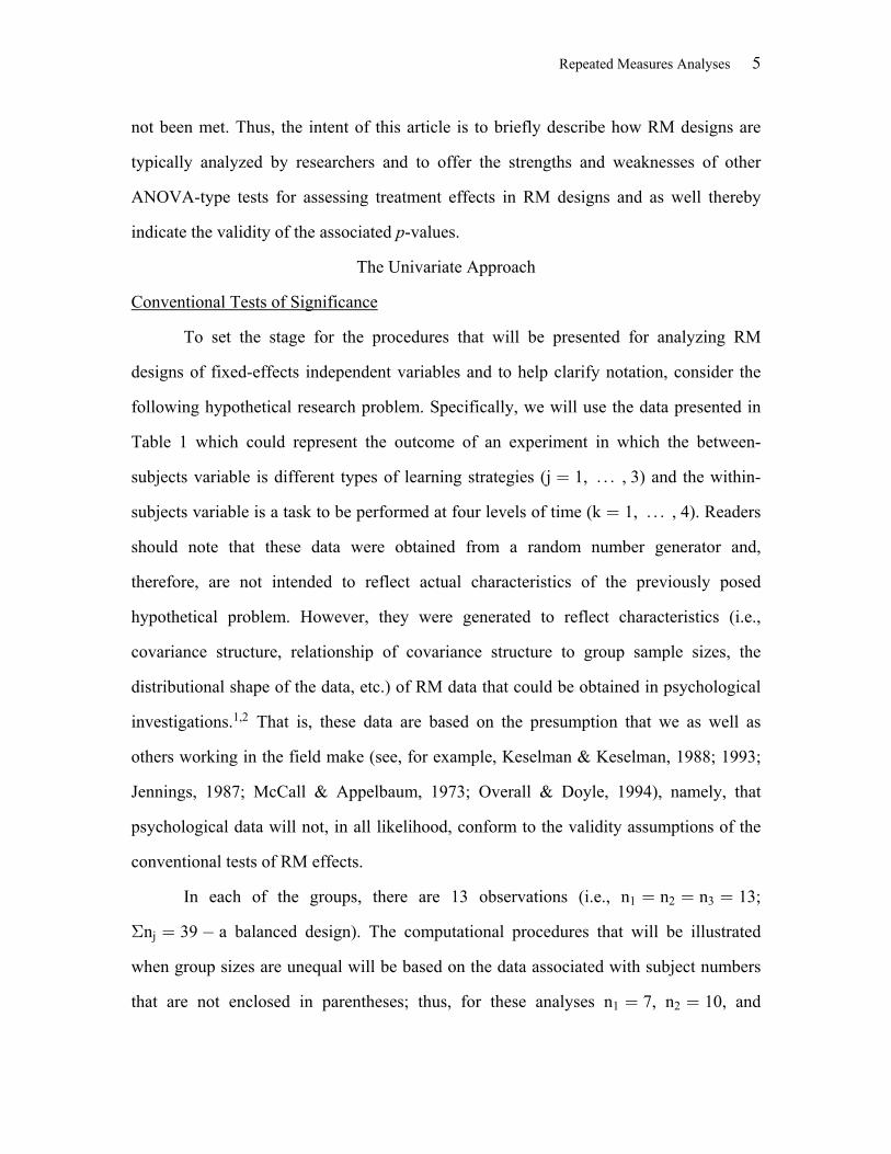
To set the stage for the procedures that will be presented for analyzing RM

designs of fixed-effects independent variables and to help clarify notation, consider the

following hypothetical research problem. Specifically, we will use the data presented in

Table 1 which could represent the outcome of an experiment in which the between-

subjects variable is different types of learning strategies (j 1, , 3) and the within-œ á

subjects variable is a task to be performed at four levels of time (k 1, , 4). Readersœ á

should note that these data were obtained from a random number generator and,

therefore, are not intended to reflect actual characteristics of the previously posed

hypothetical problem. However, they were generated to reflect characteristics (i.e.,

covariance structure, relationship of covariance structure to group sample sizes, the

distributional shape of the data, etc.) of RM data that could be obtained in psychological

investigations. That is, these data are based on the presumption that we as well as1,2

others working in the field make (see, for example, Keselman & Keselman, 1988; 1993;

Jennings, 1987; McCall & Appelbaum, 1973; Overall & Doyle, 1994), namely, that

psychological data will not, in all likelihood, conform to the validity assumptions of the

conventional tests of RM effects.

In each of the groups, there are 13 observations (i.e., n n n 13;1 2 3œ œ œ

Dn 39 a balanced design). The computational procedures that will be illustratedj œ

when group sizes are unequal will be based on the data associated with subject numbers

that are not enclosed in parentheses; thus, for these analyses n 7, n 10, and1 2œ œ


n 13 ( n 30). Cell and marginal (unweighted) means for each data set (balanced3 jœ œD

and unbalanced) are contained in Table 2.

It is important to note at the outset that we only consider one type of unbalanced

RM design, namely when unbalancedness is due to unequal between-subjects group

sizes. Thus, we do not consider unbalancedness due to missing data across the levels of

the RM variable. In some areas of psychological research (e.g., surveys over time,

longitudinal health related investigations) missing data may arise and should be dealt

with with other analyses not discussed in this paper; analyses of this sort have been

presented by Hedeker and Gibbons (1997) and Little (1995).

Tests of the within-subjects main and interaction effects conventionally have been

accomplished by the use of the univariate F statistics reported in many of our text books

(see e.g., Kirk, 1995; Maxwell & Delaney, 1990). In a design that does not include a

between-subjects grouping factor, the validity of the within-subjects main effects test

rests on the assumptions of normality, independence of errors, and homogeneity of the

treatment-difference variances (i.e., sphericity) (Huynh & Feldt, 1970; Rogan et al.,

1979; Rouanet & Lepine, 1970). Further, in the presence of a between-subjects grouping

factor the validity of the within-subjects main and interaction test require that the data

meet an additional assumption, namely, that the covariance matrices of these treatment-

difference variances are the same for all levels of this grouping factor. Jointly, these two

assumptions have been referred to as multisample sphericity (Mendoza, 1980).

When the assumptions to the conventional tests have been satisfied, they will

provide a valid test of their respective null hypotheses and will be uniformly most

powerful for detecting treatment effects when they are present. These conventional tests

are easily obtained with the major statistical packages, that is with BMDP (1994), SAS

(1990), and SPSS (Norusis, 1993). Thus, when assumptions are known to be satisfied

psychological researchers can adopt the conventional procedures and report the

associated p-values since, under these conditions, these values are an accurate reflection


of the probability of observing an F value as, or more extreme, than the observed F

statistic. For the balanced data set (i.e., N 39) given in Table 1, PROC GLM (SAS,œ

1990) results are F [3, 108] 1.54, p .21 and F [6, 108] 2.82, p .01.K J Kœ œ œ œ‚

However, McCall and Appelbaum (1973) provide a very good illustration as to

why in many areas of psychology (e.g., developmental, learning), the covariances

between the levels of the RM variable will not conform to the required covariance pattern

for a valid univariate F test. They use an example from developmental psychology to

illustrate this point. Specifically, adjacent-age assessments typically correlate more

highly than developmentally distant assessments (e.g., “IQ at age 3 correlates .83 with IQ

at age 4 but .46 with IQ at age 12”); this type of correlational structure does not

correspond to a spherical covariance structure. That is, for many psychological

paradigms successive or adjacent measurement occasions are more highly correlated than

non-adjacent measurement occasions with the correlation between these measurements

decreasing the farther apart the measurements are in the series (Danford, Hughes, &

McNee, 1960; Winer, 1971). Indeed, as McCall and Appelbaum note “Most longitudinal

studies using age or time as a factor cannot meet these assumptions.” (p. 403) McCall and

Appelbaum also indicate that the covariance pattern found in learning experiments would

also not likely conform to a spherical pattern. As they note, “ experiments in whichá

change in some behavior over short periods of time is compared under several different

treatments often cannot meet covariance requirements.” (p. 403)

The result of applying the conventional tests of significance with data that do not

conform to the assumptions of multisample sphericity will be that too many null

hypotheses will be falsely rejected (Box, 1954; Collier, et al., 1967; Imhof, 1962; Kogan,

1948; Stoloff, 1970). Furthermore, as the degree of non sphericity increases, the

conventional RM F tests becomes increasingly liberal (Noe, 1976; Rogan, et al., 1979).

For example, the results reported by Collier et. al. and Rogan et al. indicate that Type I

error rates can approach 10% for both the test of the RM main and interaction effects


when sphericity does not hold. Thus, -values are not accurate reflections of the observedp

statistics occurring by chance under their null hypotheses. Hence, using these -values top

ascertain whether the treatment has been successful or not will give a biased picture of

the nature of the treatment.

Univariate Adjusted Degrees of Freedom Tests

Greenhouse and Geisser (1959) and Huynh and Feldt (1976)-Lecoutre (1991)

When the covariance matrices for the treatment-difference variances are equal but

the common (pooled) covariance matrix is not spherical, or when the design is balanced

the Greenhouse and Geisser (1959) and Huynh and Feldt (1976) adjusted df univariate

tests are effective alternatives to the conventional tests (see also Quintana & Maxwell,

1994 for other adjusted df tests). The Greenhouse and Geisser or Huynh and Feldt

methods adjust the df of the usual F statistics; the adjustment for each approach is based

on a sample estimate, and , respectively, of the unknown sphericity parameter% %s µ

epsilon ( ). Thus, for example, whereas the value for the conventional main effect test% p

is the area beyond F in an F distribution with K 1 and (N J)(K 1) df, the valueK p

for the Greenhouse-Geisser test is the area beyond F in an F distribution with timesK %s

K 1 and times (N J)(K 1) df. s%

The empirical literature indicates that the Greenhouse and Geisser (1959) and

Huynh and Feldt (1976) adjusted df tests are robust to violations of multisample

sphericity as long as group sizes are equal (see Rogan et al., 1979). The -valuesp

associated with these statistics will provide an accurate reflection of the probability of

obtaining these adjusted statistics by chance under the null hypotheses of no treatment

effects.

The major statistical packages [BMDP, SAS, SPSS] provide Greenhouse and

Geisser (1959) and Huynh and Feldt (1976) adjusted p-values. For the balanced data set


given in Table 1, PROC GLM (SAS, 1990) results for the Greenhouse and Geisser tests

are F [3(.45) 1.34, 108(.45) 48.19] 1.54, p .23 and F [6(.45) 2.68,K J Kœ œ œ œ œ‚

108(.45) 48.19] 2.82, p .05, where .45. The corresponding Huynh andœ œ œ œs%

Feldt results are F [3(.48) 1.45, 108(.48) 52.14] 1.54, p .22 andK œ œ œ œ

F [6(.48) 2.90, 108(.48) 52.14] 2.82, p .05, where .48.J K‚ œ œ œ œ œµ%

However, the Greenhouse and Geisser (1959) and Huynh and Feldt (1976) tests

are not robust when the design is unbalanced (Algina & Oshima, 1994, 1995; Keselman,

et al., 1995; Keselman & Keselman, 1990; Keselman, Lix & Keselman, 1996).

Specifically, the tests will be conservative (liberal) when group sizes and covariance

matrices are positively (negatively) paired with one another. For example, the rates when

depressed can be lower than 1% and when liberal higher than 11% (see Keselman,

Algina, Kowalchuk & Wolfinger, in press).

In addition to the Geisser and Greenhouse (1959) and Huynh and Feldt (1976)

tests, other adjusted df tests are available for obtaining a valid test. The test to be

introduced now not only corrects for non sphericity, but as well, adjusts for heterogeneity

of the covariance matrices.

The Huynh (1978)-Algina (1994)-Lecoutre (1991) Statistic

Huynh (1978) developed a test of the within-subjects main and interaction

hypotheses, the Improved General Approximation (IGA) test, that is designed to be used

when multisample sphericity is violated. The IGA tests of the within-subjects main and

interaction hypotheses are the usual statistics, F and F , respectively, withK J K‚

corresponding critical values of bF[ ; h', h] and cF[ ; h'', h]. The parameters of the! !

critical values are defined in terms of the group covariance matrices and group sample

sizes. Estimates of the parameters and the correction due to Lecoutre (1991), are

presented in Algina (1994) and Keselman and Algina (1996). These parameters adjust the

critical value to take into account the effect that violation of multisample sphericity has

on F and F .K J K‚


The IGA tests have been found to be robust to violations of multisample

sphericity, even for unbalanced designs where the data are not multivariate normal in

form (see Keselman et al., in press; Keselman, Algina, Kowalchuk & Wolfinger, 1997).

This result is not surprising in that these tests were specifically designed to adjust for non

sphericity and heterogeneity of the between-subjects covariance matrices. Thus, the -p

values associated with the IGA tests of the RM effects are accurate.

A SAS/IML (SAS Institute, 1989) program is also available for computing this

test in any RM design (see Algina, 1997). IGA results for the unbalanced data set are

F [1.64, 34.39] 2.38, p .09, where b .88 and F [2.86, 34.39] 4.19, p .01),K J Kœ œ œ œ œs‚

where c .91.s œ

A General Method

Another procedure that researchers can adopt to test RM effects can be derived

from a general formulation for analyzing effects in RM models. This newest approach to

the analysis of repeated measurements is a mixed-model analysis. Advocates of this

approach suggest that it provides the `best' approach to the analysis of repeated

measurements since it can, among other things, handle missing data and also allows users

to model the covariance structure of the data. 3 Thus, one can use this procedure to select

the most appropriate covariance structure prior to testing the usual RM hypotheses (e.g.,

F and F ). K J K‚ The first of these advantages is typically not a pertinent issue to those

involved in controlled experiments since data in these contexts are rarely missing. The4

second consideration, however, could be most relevant to experimenters since modeling

the correct covariance structure of the data should result in more powerful tests of the

fixed-effects parameters.

The mixed approach, and specifically SAS' (SAS Institute, 1995, 1996) PROC

MIXED, allows users to fit various covariance structures to the data. For example, some

of the covariance structures that can be fit with PROC MIXED are: (a) compound

symmetric, (b) unstructured, (c) spherical, (d) first-order auto regressive, and (e) random


coefficients (see Wolfinger, 1996 for specifications of structures (a)-(e), and other,

covariance structures). The spherical structure, as indicated, is assumed by the

conventional univariate F tests in the SAS GLM program (SAS Institute, 1990), while the

unstructured covariance structure is assumed by multivariate tests of the RM effects.

First-order auto regressive and random coefficients structures reflect that measurements

that are closer in time could be more highly correlated than those farther apart in time.

The program allows even greater flexibility to the user by allowing him/her to model

covariance structures that have within-subjects and/or between-subjects heterogeneity. In

order to select an appropriate structure for one's data, PROC MIXED users can use either

an Akaike (1974) or Schwarz (1978) information criteria (see Littell et al., 1996, pp. 101-

102).

Keselman et al. (1997) recommend that users adopt the optional Satterthwaite F

tests rather than the default F tests when using PROC MIXED since they are typically

robust to violations of multisample sphericity for unbalanced heterogeneous designs in

cases where the default tests are not. Furthermore, their data indicate that the F-tests

available through PROC MIXED are generally insensitive to non normality, covariance

heterogeneity, and non sphericity when group sizes are equal.

Based on the belief that applied researchers work with data that is characterized

by both within- and between-subjects heterogeneity, eleven covariance structures were fit

to our balanced data set with PROC MIXED using both the Akaike (1974) and Schwarz

(1978) criteria; that is, we allowed these criteria to select a structure from among eleven

possible structures. Specifically, we allowed PROC MIXED to select from among

homogeneous, within heterogeneous, and within- and between-heterogeneous structures.

From the eleven structures fit to the data, the Akaike criterion selected an unstructured

within-subjects covariance structure in which this type of within-subjects structure varied

across groups (i.e., between-heterogeneous structure). The Schwarz criterion also

selected an unstructured within-subjects covariance structure, however, it did not pick the


between-heterogeneous version of this structure as did Akaike. The F-tests based on the

Akaike selection were F [3, 28.38] 3.61, p .03 and F [6, 23.70] 4.43, p .00.K J Kœ œ œ œ‚

The corresponding values based on the Schwarz criterion were F [3, 36] 3.61, p .02K œ œ

and F [6, 36] 3.06, p .02.J K‚ œ œ

The Multivariate Approach

The multivariate test of the RM main effect in a between- by within-subjects

design is performed by creating K 1 difference (D) variables. The null hypothesis that

is tested, using Hotelling's (1931) T statistic, is that the vector of population means of2

these K 1 D variables equals the null vector (see McCall & Appelbaum, 1973, for a

fuller discussion and example).

The multivariate test of the within-subjects interaction effect, on the other hand, is

a test of whether the vector of population means of the K 1 D variables are equal

across the levels of the grouping variable. A test of this hypothesis can be obtained by

conducting a one-way multivariate ANOVA, where the K 1 D variables are the

dependent variables and the grouping variable (J) is the between-subjects independent

variable. When J 2 four popular multivariate criteria are: (1) Wilk's (1932) likelihood

ratio, (2) the Pillai (1955)-Bartlett (1939) trace statistic, (3) Roy's (1953) largest root

criterion, and (4) the Hotelling (1951)-Lawley (1938) trace criterion. When J 2, allœ

criteria are equivalent to Hotelling's T statistic.2

Valid multivariate tests of the RM hypotheses in between- by within-subjects

designs, unlike the univariate tests, depend not on the sphericity assumption, but only on

the equality of the covariance matrices at all levels of the grouping factor as well as

normality and independence of observations across subjects.

The empirical results indicate that the multivariate test of the RM main effect is

generally robust to assumption violations when the design is balanced (or contains no

grouping factors) and not robust when the design is unbalanced (Algina & Oshima, 1994;


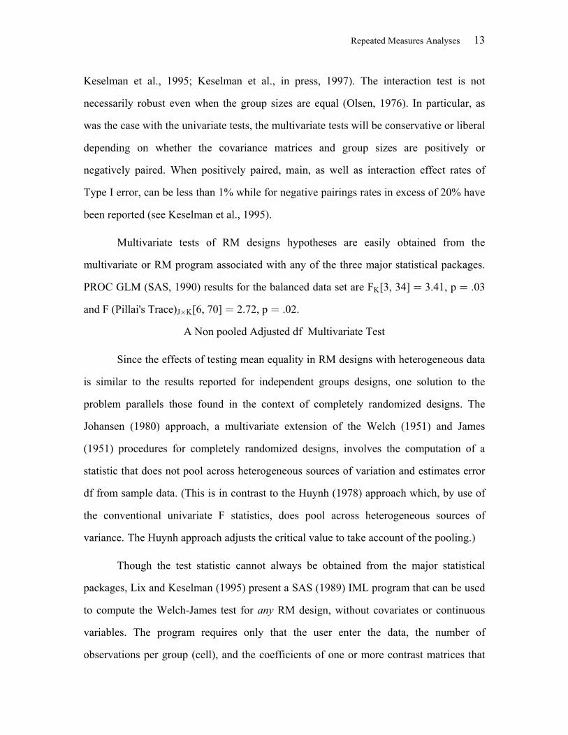
Keselman et al., 1995; Keselman et al., in press, 1997). The interaction test is not

necessarily robust even when the group sizes are equal (Olsen, 1976). In particular, as

was the case with the univariate tests, the multivariate tests will be conservative or liberal

depending on whether the covariance matrices and group sizes are positively or

negatively paired. When positively paired, main, as well as interaction effect rates of

Type I error, can be less than 1% while for negative pairings rates in excess of 20% have

been reported (see Keselman et al., 1995).

Multivariate tests of RM designs hypotheses are easily obtained from the

multivariate or RM program associated with any of the three major statistical packages.

PROC GLM (SAS, 1990) results for the balanced data set are F [3, 34] 3.41, p .03K œ œ

and F (Pillai's Trace) [6, 70] 2.72, p .02.J K‚ œ œ

A Non pooled Adjusted df Multivariate Test

Since the effects of testing mean equality in RM designs with heterogeneous data

is similar to the results reported for independent groups designs, one solution to the

problem parallels those found in the context of completely randomized designs. The

Johansen (1980) approach, a multivariate extension of the Welch (1951) and James

(1951) procedures for completely randomized designs, involves the computation of a

statistic that does not pool across heterogeneous sources of variation and estimates error

df from sample data. (This is in contrast to the Huynh (1978) approach which, by use of

the conventional univariate F statistics, does pool across heterogeneous sources of

variance. The Huynh approach adjusts the critical value to take account of the pooling.)

Though the test statistic cannot always be obtained from the major statistical

packages, Lix and Keselman (1995) present a SAS (1989) IML program that can be used

to compute the Welch-James test for RM design, without covariates or continuousany

variables. The program requires only that the user enter the data, the number of

observations per group (cell), and the coefficients of one or more contrast matrices that


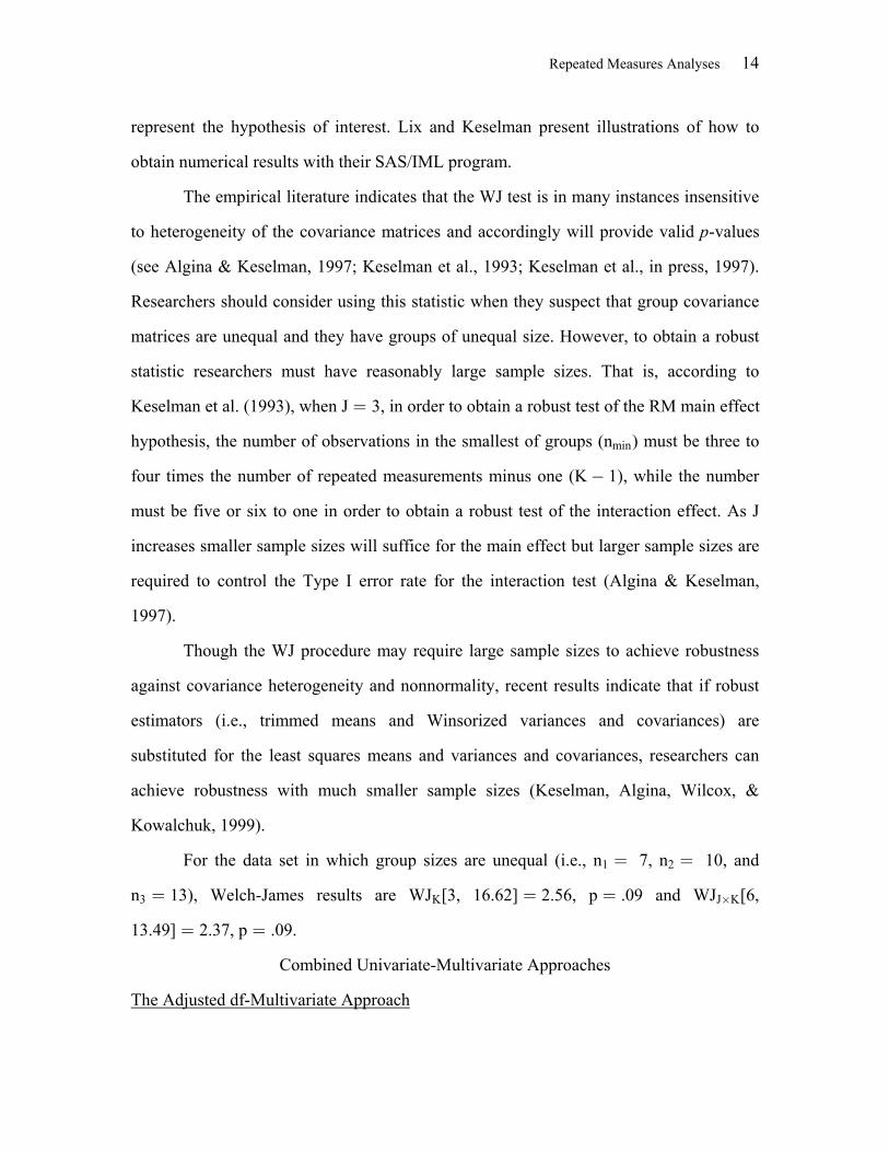
represent the hypothesis of interest. Lix and Keselman present illustrations of how to

obtain numerical results with their SAS/IML program.

The empirical literature indicates that the WJ test is in many instances insensitive

to heterogeneity of the covariance matrices and accordingly will provide valid -valuesp

(see Algina & Keselman, 1997; Keselman et al., 1993; Keselman et al., in press, 1997).

Researchers should consider using this statistic when they suspect that group covariance

matrices are unequal and they have groups of unequal size. However, to obtain a robust

statistic researchers must have reasonably large sample sizes. That is, according to

Keselman et al. (1993), when J 3, in order to obtain a robust test of the RM main effectœ

hypothesis, the number of observations in the smallest of groups (n ) must be three tomin

four times the number of repeated measurements minus one (K 1), while the number

must be five or six to one in order to obtain a robust test of the interaction effect. As J

increases smaller sample sizes will suffice for the main effect but larger sample sizes are

required to control the Type I error rate for the interaction test (Algina & Keselman,

1997).

Though the WJ procedure may require large sample sizes to achieve robustness

against covariance heterogeneity and nonnormality, recent results indicate that if robust

estimators (i.e., trimmed means and Winsorized variances and covariances) are

substituted for the least squares means and variances and covariances, researchers can

achieve robustness with much smaller sample sizes (Keselman, Algina, Wilcox, &

Kowalchuk, 1999).

For the data set in which group sizes are unequal (i.e., n 7, n 10, and1 2œ œ

n 13), Welch-James results are WJ [3, 16.62] 2.56, p .09 and WJ [6,3 K J Kœ œ œ ‚

13.49] 2.37, p .09.œ œ

Combined Univariate-Multivariate Approaches

The Adjusted df-Multivariate Approach


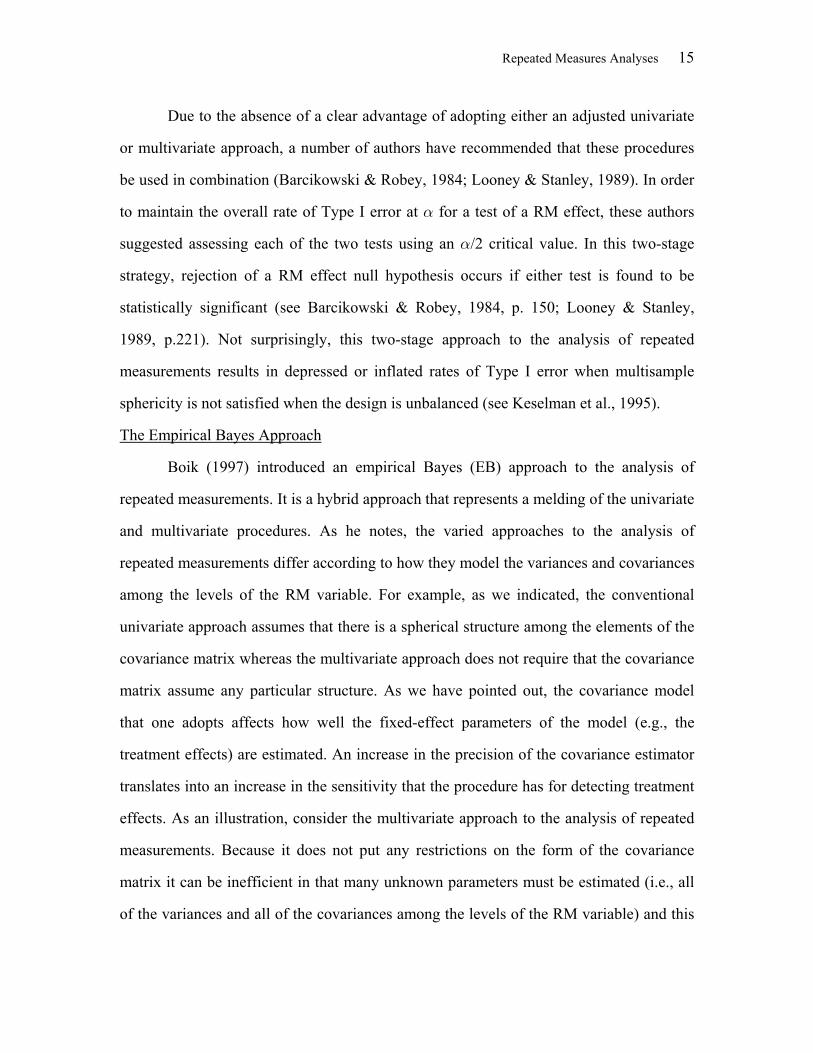
Due to the absence of a clear advantage of adopting either an adjusted univariate

or multivariate approach, a number of authors have recommended that these procedures

be used in combination (Barcikowski & Robey, 1984; Looney & Stanley, 1989). In order

to maintain the overall rate of Type I error at for a test of a RM effect, these authors!

suggested assessing each of the two tests using an /2 critical value. In this two-stage!

strategy, rejection of a RM effect null hypothesis occurs if either test is found to be

statistically significant (see Barcikowski & Robey, 1984, p. 150; Looney & Stanley,

1989, p.221). Not surprisingly, this two-stage approach to the analysis of repeated

measurements results in depressed or inflated rates of Type I error when multisample

sphericity is not satisfied when the design is unbalanced (see Keselman et al., 1995).

The Empirical Bayes Approach

Boik (1997) introduced an empirical Bayes (EB) approach to the analysis of

repeated measurements. It is a hybrid approach that represents a melding of the univariate

and multivariate procedures. As he notes, the varied approaches to the analysis of

repeated measurements differ according to how they model the variances and covariances

among the levels of the RM variable. For example, as we indicated, the conventional

univariate approach assumes that there is a spherical structure among the elements of the

covariance matrix whereas the multivariate approach does not require that the covariance

matrix assume any particular structure. As we have pointed out, the covariance model

that one adopts affects how well the fixed-effect parameters of the model (e.g., the

treatment effects) are estimated. An increase in the precision of the covariance estimator

translates into an increase in the sensitivity that the procedure has for detecting treatment

effects. As an illustration, consider the multivariate approach to the analysis of repeated

measurements. Because it does not put any restrictions on the form of the covariance

matrix it can be inefficient in that many unknown parameters must be estimated (i.e., all

of the variances and all of the covariances among the levels of the RM variable) and this


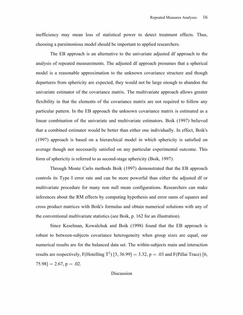
inefficiency may mean loss of statistical power to detect treatment effects. Thus,

choosing a parsimonious model should be important to applied researchers.

The EB approach is an alternative to the univariate adjusted df approach to the

analysis of repeated measurements. The adjusted df approach presumes that a spherical

model is a reasonable approximation to the unknown covariance structure and though

departures from sphericity are expected, they would not be large enough to abandon the

univariate estimator of the covariance matrix. The multivariate approach allows greater

flexibility in that the elements of the covariance matrix are not required to follow any

particular pattern. In the EB approach the unknown covariance matrix is estimated as a

linear combination of the univariate and multivariate estimators. Boik (1997) believed

that a combined estimator would be better than either one individually. In effect, Boik's

(1997) approach is based on a hierarchical model in which sphericity is satisfied on

average though not necessarily satisfied on any particular experimental outcome. This

form of sphericity is referred to as second-stage sphericity (Boik, 1997).

Through Monte Carlo methods Boik (1997) demonstrated that the EB approach

controls its Type I error rate and can be more powerful than either the adjusted df or

multivariate procedure for many non null mean configurations. Researchers can make

inferences about the RM effects by computing hypothesis and error sums of squares and

cross product matrices with Boik's formulas and obtain numerical solutions with any of

the conventional multivariate statistics (see Boik, p. 162 for an illustration).

Since Keselman, Kowalchuk and Boik (1998) found that the EB approach is

robust to between-subjects covariance heterogeneity when group sizes are equal, our

numerical results are for the balanced data set. The within-subjects main and interaction

results are respectively, F(Hotelling T ) [3, 36.99] 3.32, p .03 and F(Pillai Trace) [6,2 œ œ

75.98] 2.67, p .02.œ œ

Discussion


The intent of this paper was to indicate that “repeated measures ANOVA” can

refer to a number of different type of analyses for RM designs. Specifically, we indicated

that RM ANOVA could be construed to mean the conventional tests of significance, the

adjusted df univariate test statistics, a multivariate analysis, a multivariate analysis that

does not require the assumptions associated with the usual multivariate test, or a

combined univariate-multivariate test. In addition, by indicating the strengths and

weaknesses of each of these approaches we intended to convey the validity or lack there

of that can be associated with the -values corresponding with each of these approaches.p

Thus, researchers can better convey the validity of their findings by indicating the type of

“repeated measures ANOVA” that was used to assess treatment effects.

In conclusion, we and others (Keselman & Keselman, 1988; 1993; Jennings,

1987; McCall & Appelbaum, 1973; Overall & Doyle, 1994) feel it is rarely legitimate to

use the conventional tests of significance since data are not likely to conform to the very

strict assumptions associated with this procedure. On the other hand, researchers should

take comfort in the fact that there are many viable alternatives to the conventional tests of

significance. Furthermore, we believe that we can offer simple guidelines for choosing

between them, guidelines which, by in large, are based on whether group sizes are equal

or not. That is, for RM designs containing no between-subjects variables or for between-5

by within-subjects designs having groups of equal size, we recommend either the

empirical Bayes or the mixed-model approach. Boik (1997) demonstrated that his

approach will typically provide more powerful tests of RM effects as compared to

uniformly adopting either an adjusted df univariate approach or a multivariate test

statistic. Furthermore, numerical results can easily be obtained with a standard

multivariate program. The mixed-model approach also will likely provide more powerful

tests of RM effects compared to the adjusted df univariate and multivariate approaches

because researchers can model the covariance structure of their data. Furthermore, for

designs that contain between-subjects grouping variables, heterogeneity across the levels


of the grouping variable can also be modeled. To the extent that the actual covariance

structure of the data resembles the fit structure, it is likely that the mixed-model approach

will provide more powerful tests than the empirical Bayes approach; however, this

observation has not yet been confirmed through empirical investigation. A caveat to this

recommendation is that when covariance matrices are suspected to be unequal a likelier

safer course of action, in terms of Type I error protection, is to use an adjusted-df

univariate test. That is, some findings suggest that the EB and mixed model approaches6

may result in inflated rates of Type I error when covariance matrices are unequal and

sample sizes are small, even when group sizes are equal (see Keselman et al, in press,

1997; Keselman, Kowalchuk & Boik, 1998; Wright & Wolfinger, 1996).

In those (fairly typical) cases where the group sizes are unequal and one does not

know that the group covariance matrices are equal, researchers should use either the IGA

or Welch-James tests. Based upon power analyses, it appears that the WJ test can have

substantial power advantages over the IGA test (Algina & Keselman, 1998). The

SAS/IML (1989) program presented by Lix and Keselman (1995) can be used to obtain

numerical results. However, according to results provided by Keselman et al (1993) and

Algina and Keselman (1997) sample sizes cannot be small. When sample sizes are

unequal and small, we recommend the IGA test.

When researchers feel that they are dealing with populations that are nonnormal

in form [Tukey (1960) suggests that most populations are skewed and/or contain outliers]

and thus prescribe to the position that inferences pertaining to robust parameters are more

valid than inferences pertaining to the usual least squares parameters, then either the IGA

or WJ procedures, based on robust estimators, can be adopted. Results provided by

Keselman et al., (1999) certainly suggest that these procedures will provide valid tests of

the RM main and interaction effect hypotheses (of trimmed population means) when data

are non-normal, nonspherical, and heterogeneous. A limitation to this recommendation

however is that, to date, software is not generally available for obtaining numerical


results, though the program provided by Lix and Keselman (1995) can be modified to

work with robust estimators.

As a postscript the reader should note that the mixed-model, WJ, and EB

approaches can also be applied to tests of contrasts (see e.g., SAS Institute, 1992, Ch. 16;

Lix & Keselman, 1995; Boik, 1997). Readers can also consult Hertzog and Rovine

(1985), Keselman, Keselman and Shaffer (1991), Lix and Keselman (1996), and

Keselman and Algina (1996) regarding contrast testing in RM designs.


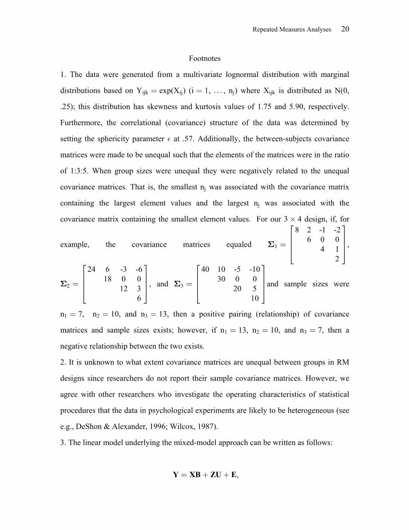
Footnotes

1. The data were generated from a multivariate lognormal distribution with marginal

distributions based on Y exp(X ) (i 1, , n ) where X is distributed as N(0,ijk ij j ijkœ œ á

.25); this distribution has skewness and kurtosis values of 1.75 and 5.90, respectively.

Furthermore, the correlational (covariance) structure of the data was determined by

setting the sphericity parameter at .57. Additionally, the between-subjects covariance%

matrices were made to be unequal such that the elements of the matrices were in the ratio

of 1:3:5. When group sizes were unequal they were negatively related to the unequal

covariance matrices. That is, the smallest n was associated with the covariance matrixj

containing the largest element values and the largest n was associated with thej

covariance matrix containing the smallest element values. For our 3 4 design, if, for‚

example, the covariance matrices equaled ,

8 2 -1 -26 0 0

4 12

D1 œ

Ô ×Ö ÙÖ ÙÕ Ø

D D2 3œ œ

Ô × Ô ×Ö Ù Ö ÙÖ Ù Ö ÙÕ Ø Õ Ø

24 6 -3 -6 40 10 -5 -1018 0 0 30 0 0

12 3 20 56 10

, and and sample sizes were

n 7, n 10, and n 13, then a positive pairing (relationship) of covariance1 2 3œ œ œ

matrices and sample sizes exists; however, if n 13, n 10, and n 7, then a1 2 3œ œ œ

negative relationship between the two exists.

2. It is unknown to what extent covariance matrices are unequal between groups in RM

designs since researchers do not report their sample covariance matrices. However, we

agree with other researchers who investigate the operating characteristics of statistical

procedures that the data in psychological experiments are likely to be heterogeneous (see

e.g., DeShon & Alexander, 1996; Wilcox, 1987).

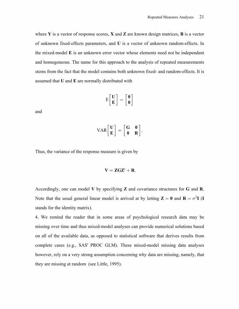
3. The linear model underlying the mixed-model approach can be written as follows:

Y XB ZU Eœ ,


where is a vector of response scores, and are known design matrices, is a vectorY X Z B

of unknown fixed-effects parameters, and is a vector of unknown random-effects. InU

the mixed-model is an unknown error vector whose elements need not be independentE

and homogeneous. The name for this approach to the analysis of repeated measurements

stems from the fact that the model contains both unknown fixed- and random-effects. It is

assumed that and are normally distributed withU E

E” • ” •U 0E 0œ

and

VAR .” • ” •U G 0E 0 Rœ

Thus, the variance of the response measure is given by

V ZGZ Rœ w .

Accordingly, one can model by specifying and covariance structures for and .V Z G R

Note that the usual general linear model is arrived at by letting and (Z 0 R I Iœ œ 52

stands for the identity matrix).

4. We remind the reader that in some areas of psychological research data may be

missing over time and thus mixed-model analyses can provide numerical solutions based

on all of the available data, as opposed to statistical software that derives results from

complete cases (e.g., SAS' PROC GLM). These mixed-model missing data analyses

however, rely on a very strong assumption concerning why data are missing, namely, that

they are missing at random (see Little, 1995).


5. We caution the reader that our recommendations are no substitute for carefully

examining the characteristics of their data and basing their choice of a test statistic on this

examination. There are a myriad of factors (e.g., scale of measurement, distribution

shape, outliers, etc.) that we have not considered for the sake of simplicity in formulating

our recommendations which could result in other data analysis choices (e.g., non

parametric analyses, analyses based on robust estimators rather than least squares

estimators, transformations of the data, etc.). Furthermore, the empirical literature that

has been published regarding the efficacy of the new procedures reviewed in this paper is

extremely limited and accordingly future findings may result in better recommendations.

6. As we indicated, it is unknown to what extent covariance matrices are unequal

between groups in RM designs since researchers do not report their sample covariance

matrices. The safest course of action, when group sizes are unequal, is to adopt a

procedure that allows for heterogeneity. The empirical literature also indicates that one

will not suffer substantial power loses by using a heterogeneous test statistic when

heterogeneity does not exist (see e.g., Algina & Keselman, 1998; Keselman et al., 1997).


Acknowledgments

Work on this paper was supported by grants from the Natural Sciences and

Engineering Research Council of Canada and the Social Sciences and Humanities

Research Council of Canada.


References

Akaike, H. (1974). A new look at the statistical model identification. IEEE

Transaction on Automatic Control, , 716-723.AC-19

Algina, J. (1997). Generalization of improved general approximation tests to split-

plot designs with multiple between-subjects factors and/or multiple within-subjects

factors. , , 243-252.British Journal of Mathematical and Statistical Psychology 50

Algina, J. (1994). Some alternative approximate tests for a split plot design.

Multivariate Behavioral Research 29, , 365-384.

Algina, J., & Coombs, W. T. (1996). A review of selected parametric solutions to the

Behrens-Fisher problem. In B Thompson's (Ed) Advances in social science methodology

(Vol 4), Greenwich, Conn: JAI Press.

Algina, J., & Keselman, H. J. (1998). A power comparison of the Welch-James and

Improved General Approximation tests in the split-plot design. Journal of Educational

and Behavioral Statistics 23, , 152-169.

Algina, J., & Keselman, H. J. (1997). Testing repeated measures hypotheses when

covariance matrices are heterogeneous: Revisiting the robustness of the Welch-James

test. , , 255-274.Multivariate Behavioral Research 32

Algina, J., & Oshima, T. C. (1994). Type I error rates for Huynh's general

approximation and improved general approximation tests. British Journal of

Mathematical and Statistical Psychology 47, , 151-165.

Algina, J., & Oshima, T. C. (1995). An improved general approximation test for the

main effect in a split-plot design. British Journal of Mathematical and Statistical

Psychology 48, , 149-160.

Barcikowski, R. S., & Robey, R. R. (1984). Decisions in single group repeated

measures analysis: Statistical tests and three computer packages. The American

Statistician 38, , 148-150.


Bartlett, M. S. (1939). A Note on tests of significance in multivariate analysis.

Proceedings of the Cambridge Philosophical Society, , 180-185.35

BMDP Statistical Software Inc. (1994) . BMDP New System for Windows, Version

1. Author, Los Angeles.

Boik, R. J. (1997). Analysis of repeated measures under second-stage sphericity: An

empirical Bayes approach. , , 155-Journal of Educational and Behavioral Statistics 22

192.

Box, G.E.P. (1954). Some theorems on quadratic forms applied in the study of

analysis of variance problems, I. Effects of inequality of variance in the one-way

classification. , 290-302.Annals of Mathematical Statistics 25,

Collier, R. O. Jr., Baker, F. B., Mandeville, G. K., & Hayes, T. F. (1967). Estimates

of test size for several test procedures based on conventional variance ratios in the

repeated measures design. , , 339-353.Psychometrika 32

Danford, M. B., Hughes, H. M., & McNee, R. C. (1960). On the analysis of repeated-

measurements experiments. , , 547-565.Biometrics 16

DeShon, R. P., & Alexander, R.A. (1996). Alternative procedures for testing

regression slope homogeneity when group error variances are unequal. Psychological

Methods 1, , 261-277.

Greenhouse, S. W. & Geisser, S. (1959). On methods in the analysis of profile data.

Psychometrika 24, , 95-112.

Hedeker, D., & Gibbons, R.D. (1997). Application of random-effects pattern-mixture

models for missing data in longitudinal studies. , , 64-78.Psychological Methods 2

Hertzog, C., & Rovine, M. (1985). Repeated-measures analysis of variance in

developmental research: Selected issues. , , 787-809.Child Development 56

Hotelling, H. (1931). The generalization of Student's ratio. Annals of Mathematical

Statistics, , 360-378.2


Hotelling, H. (1951). “A Generalized Test and Measure of Multivariate Dispersion,”t

In J. Neyman (Ed.). Proceedings of the Second Berkeley Symposium on Mathematical

Statistics and Probability, University of California Press, Berkeley, , 23-41.2

Huynh, H. (1978). Some approximate tests for repeated measurement designs.


Huynh, H. & Feldt, L. (1970). Conditions under which mean square ratios in repeated

measurements designs have exact F distributions. Journal of the American Statistical

Association, , 1582-1589.65

Huynh, H. & Feldt, L. S. (1976). Estimation of the Box correction for degrees of

freedom from sample data in randomized block and split-plot designs. Journal of

Educational Statistics, , 69-82.1

Imhof, J. P. (1962). Testing the hypothesis of no fixed main-effects in Scheffe's

mixed model. , , 1085-1095.Annals of Mathematical Statistics 33

James, G. S. (1951). The comparison of several groups of observations when the

ratios of the population variances are unknown. , , 324-329.Biometrika 38

Jennings, J.R. (1987). Editorial policy on analyses of variance with repeated

measures. , , 474-475.Psychophysiology 24

Johansen, S. (1980). The Welch-James approximation to the distribution of the

residual sum of squares in a weighted linear regression. , , 85-92.Biometrika 67

Keselman, H. J. & Algina, J. (1996). The analysis of higher-order repeated measures

designs. In B Thompson's (Ed) ,Advances in social science methodology (Vol 4)

Greenwich, Conn: JAI Press.

Keselman, H. J., Algina, J., Wilcox, R. R., & Kowalchuk, R. K. (1999). Testing

repeated measures hypotheses when covariance matrices are heterogeneous: Revisiting

the robustness of the Welch-James test again. Manuscript submitted for publication.


Keselman, H. J., Algina, J., Kowalchuk, R. K., & Wolfinger, R. D. (in press). A

comparison of recent approaches to the analysis of repeated measurements. British

Journal of Mathematical and Statistical Psychology.

Keselman, H. J., Algina, J., Kowalchuk, R. K., & Wolfinger, R. D. (1997). The

analysis of repeated measurements with mixed-model Satterthwaite F tests . Manuscript

under review.

Keselman, H. J., Carriere, K. C., & Lix, L. M. (1993). Testing repeated measures

hypotheses when covariance matrices are heterogeneous. Journal of Educational

Statistics 18, , 305-319.

Keselman, H. J., Huberty, C. J., Lix, L. M., Olejnik, S., Cribbie, R. A., Donahue, B.,

Kowalchuk, R. K., Lowman, L. L., Petoskey, M. D., Keselman, J. C., & Levin, J. R.

(1998). Statistical practices of Educational Researchers: An analysis of their ANOVA,

MANOVA and ANCOVA analyses. , , 350-386.Review of Educational Research 68(3)

Keselman, H. J. & Keselman, J. C. (1988). Comparing repeated measures means in

factorial designs. , , 612-618.Psychophysiology 25

Keselman, H. J. & Keselman, J. C. (1993). Analysis of repeated measurements. In

L.K. Edwards (Ed.) , 105-145, MarcelApplied analysis of variance in behavioral science

Dekker, New York.

Keselman, H. J., Keselman, J. C., & Lix, L. M. (1995). The analysis of repeated

measurements: Univariate tests, multivariate tests, or both? British Journal of

Mathematical and Statistical Psychology 48, , 319-338.

Keselman, H. J., Keselman, J. C., & Shaffer, J. P. (1991). Multiple pairwise

comparisons of repeated measures means under violations of multisample sphericity.

Psychological Bulletin 110, , 162-170.

Keselman, H. J., Kowalchuk, R. K., & Boik, R. J. (1998). An investigation of the

Empirical Bayes approach to the analysis of repeated measurements. Manuscript under

review.


Keselman, H. J., Rogan, J. C., & Games, P. A. (1981). Robust tests of repeated

measures means in educational and psychological research. Educational and

Psychological Measurement 41, , 163-173.

Keselman, J. C. & Keselman, H. J. (1990). Analysing unbalanced repeated measures

designs. , , 265-282.British Journal of Mathematical and Statistical Psychology 43

Keselman, J. C., Lix, L. M., & Keselman, H. J. (1996). The analysis of repeated

measuremenmts: A quantitative research synthesis. British Journal of Mathematical and

Statistical Psychology 49, , 275-298.

Kirk, R. E. (1995). (3rdExperimental design: Procedures for the behavioral sciences

ed). Belmont, CA: Brooks/Cole.

Kogan, L. S. (1948). Analysis of variance: Repeated measurements. Psychological

Bulletin 45, , 131-143.

Lawley, D. N. (1938). A generalization of Fisher's z test. , 180-187,Biometrika, 30

467-469.

Lecoutre, B. (1991). A correction for the approximate test in repeated measures%µ

designs with two or more independent groups. , , 371-Journal of Educational Statistics 16

372.

Littell, R. C., Milliken, G. A., Stroup, W. W., & Wolfinger, R. D. (1996). SAS

system for mixed models, Cary, NC: SAS Institute.

Little, R.J.A. (1995). Modeling the drop-out mechanism in repeated-measures studies.

Journal of the American Statistical Association 90, , 1112-1121.

Lix, L. M., & Keselman, H. J. (1996). Interaction contrasts in repeated measures

designs. , , 147-162.British Journal of Mathematical and Statistical Psychology 49

Lix, L. M., & Keselman, H. J. (1995). Approximate degrees of freedom tests: A

unified perspective on testing for mean equality. , , 547-560.Psychological Bulletin 117

Looney, S. W., & Stanley, W. B. (1989). Exploratory repeated measures analysis for

two or more groups: Review and update. , , 220-225.The American Statistician 43


Maxwell, S. E., & Delaney, H. D. (1990). Designing experiments and analyzing data:

A model comparison perspective. Belmont, CA: Wadsworth.

McCall, R. B., & Appelbaum, M. I. (1973). Bias in the analysis of repeated-measures

designs: Some alternative approaches. , , 401-415.Child Development 44

Mendoza, J. L. (1980). A Significance test for multisample sphericity.


Noe, M. J. (1976). “A Monte Carlo Survey of Several Test Procedures in the

Repeated Measures Design,” Paper presented at the meeting of the American Educational

Research Association, April, San Francisco, California.

Norusis, M. J. (1993). . SPSSSPSS for Windows, Advanced Statistics, Release 6.0

Inc., Chicago, Il.

Olson, C. L. (1974). Comparative robustness of six tests in multivariate analysis of

variance. , , 894-908.Journal of the American Statistical Association 69

Overall, J.E., & Doyle, S.R. (1994). Estimating sample sizes for repeated

measurement designs. , 100-123.Controlled Clinical Trials 15 ,

Pillai, K. C. S. (1955). Some new test criteria in multivariate analysis. Annals of

Mathematical Statistics, , 117-121.26

Quintana, S. M., & Maxwell, S. E. (1994). A Monte Carlo comparison of seven -%

adjustment procedures in repeated measures designs with small sample sizes. Journal of

Educational Statistics 19, , 57-71.

Rogan, J. C., Keselman, H. J., & Mendoza, J. L. (1979). Analysis of repeated

measurements. , , 269-286.British Journal of Mathematical and Statistical Psychology 32

Rouanet, H. & Lepine, D. (1970). Comparison between treatments in a repeated

measures design: ANOVA and multivariate methods. British Journal of Mathematical

and Statistical Psychology, , 147-163.23

Roy, S. N. (1953). On a heuristic method of test construction and its use in

multivariate analysis. , , 220-238.Annals of Mathematical Statistics 24


SAS Institute. (1990). SAS/STAT User's Guide, Version 6, Fourth Edition Volume 2.

Author, Cary, NC.

SAS Institute. (1996). SAS/STAT Software: Changes and Enhancements through

release 6.11. Author, Cary, NC.

SAS Institute. (1995). . Author, Cary, NC.Introduction to the MIXED procedure

SAS Institute. (1992). SAS Technical Report: SAS/STAT Software Change and

Enhancements Release 6.07. Author, Cary, NC.

SAS Institute. (1989). . Author,SAS/IML sowtware: Usage and reference, Version 6

Cary, NC.

Schwarz, G. (1978). Estimating the dimension of a model. , ,Annals of Statistics 6

461-464.

Stoloff, P. H. (1970). Correcting for heterogeneity of covariance for repeated

measures designs of the analysis of variance. Educational and Psychological

Measurement, , 909-924.30

Tukey, J.W. (1960). A survey of sampling from contaminated normal distributions. In

I. Olkin et al. (Eds) , Stanford, CA: StanfordContributions to probability and statistics

University Press.

Welch, B. Tukey, J.W. (1960). A survey of sampling from contaminated normal

distributions. In I. Olkin et al. (Eds) , Stanford,Contributions to probability and statistics

CA: Stanford University Press.L. (1951). On the comparison of several mean values: An

alternative approach. , , 330-336.Biometrika 38

Wilcox, R. R. (1987). New designs in analysis of variance. Annual Review of

Psychology 38, , 29-60.

Wilks, S. S. (1932). Certain generalizations in the analysis of variance. ,Biometrika

24, 471-494.

Winer, B. J. (1971). , (2nd ed.). NewStatistical principles in experimental design

York: McGraw-Hill.


Wolfinger, R. D. (1996). Heterogeneous variance-covariance structures for repeated

measures. , , 205-230.Journal of Agricultural, Biological, and Environmental Statistics 1

Wright, S. P., & Wolfinger, R. D. (1996) Þ Repeated measures analysis using mixed

models: Some simulation results, Paper presented at the Conference on Modelling

Longitudinal and Spatially Correlated Data: Methods, Applications, and Future

Directions, Nantucket, MA (October).

Documents

The Analysis of Repeated Measures Designs: A Review