CHAPTER 14vulstats.ucsd.edu/pdf/Howell.ch-14.repeated-measures.pdf · CHAPTER 14 Repeated-Measures Designs Objectives To discuss the analysis of variance by considering experimental

CHAPTER 14

Repeated-MeasuresDesigns

Object ives

To discuss the analysis of variance by considering experimental designsin which the same subject is measured under all levels of one or moreindependent variables.

Contents

14.1 The Structural Model14.2 F Ratios14.3 The Covariance Matrix14.4 Analysis of Variance Applied to Relaxation Therapy14.5 Contrasts and Effect Sizes in Repeated Measures Designs14.6 Writing Up the Results14.7 One Between-Subjects Variable and One Within-Subjects Variable14.8 Two Between-Subjects Variables and One Within-Subjects Variable14.9 Two Within-Subjects Variables and One Between-Subjects Variable14.10 Intraclass Correlation14.11 Other Considerations14.12 Mixed Models for Repeated-Measures Designs

461

IN OUR DISCUSSION OF THE ANALYSIS OF VARIANCE, we have concerned ourselves with exper-imental designs that have different subjects in the different cells. More precisely, we havebeen concerned with designs in which the cells are independent, or uncorrelated. (Underthe assumptions of the analysis of variance, independent and uncorrelated are synonymousin this context.) In this chapter we are going to be concerned with the problem of analyzingdata where some or all of the cells are not independent. Such designs are somewhat morecomplicated to analyze, and the formulae become more complex. Most, or perhaps evenall, readers will approach the problem using computer software such as SPSS or SAS.However, to understand what you are seeing, you need to know something about how youwould approach the problem by hand; and that leads to lots and lots of formulae. I urge youto treat the formulae lightly, and not feel that you have to memorize any of them. Thischapter needs to be complete, and that means we have to go into the analysis at some depth,but remember that you can always come back to the formulae when you need them, anddon’t worry about the calculations too much until you do need them.

If you think of a typical one-way analysis of variance with different subjects servingunder the different treatments, you would probably be willing to concede that the correla-tions between treatments 1 and 2, 1 and 3, and 2 and 3 have an expectation of zero.

Treatment 1 Treatment 2 Treatment 3

However, suppose that in the design diagrammed here the same subjects were used inall three treatments. Thus, instead of 3n subjects measured once, we have n subjects meas-ured three times. In this case, we would be hard put to believe that the intercorrelations ofthe three treatments would have expectancies of zero. On the contrary, the better subjectsunder treatment 1 would probably also perform well under treatments 2 and 3, and thepoorer subjects under treatment 1 would probably perform poorly under the other condi-tions, leading to significant correlations among treatments.

This lack of independence among the treatments would cause a serious problem if itwere not for the fact that we can separate out, or partition, and remove the dependence im-posed by repeated measurements on the same subjects. (To use a term that will becomemuch more familiar in Chapter 15, we can say that we are partialling out effects that causethe dependence.) In fact, one of the main advantages of repeated-measures designs is thatthey allow us to reduce overall variability by using a common subject pool for all treat-ments, and at the same time allow us to remove subject differences from our error term,leaving the error components independent from treatment to treatment or cell to cell.

As an illustration, consider the highly exaggerated set of data on four subjects overthree treatments presented in Table 14.1. Here the dependent variable is the number of tri-als to criterion on some task. If you look first at the treatment means, you will see someslight differences, but nothing to get too excited about. There is so much variability withineach treatment that it would at first appear that the means differ only by chance. But lookat the subject means. It is apparent that subject 1 learns quickly under all conditions, andthat subjects 3 and 4 learn remarkably slowly. These differences among the subjects areproducing most of the differences within treatments, and yet they have nothing to do withthe treatment effect. If we could remove these subject differences we would have a better(and smaller) estimate of error. At the same time, it is the subject differences that are creat-ing the high positive intercorrelations among the treatments, and these too we will partialout by forming a separate term for subjects.

X3nX2nX1n

ÁÁÁX32X22X12

X31X21X11

462 Chapter 14 Repeated-Measures Designs

partition

partialling out

repeated-measures designs

One laborious way to do this would be to put all the subjects’ contributions on a com-mon footing by equating subject means without altering the relationships among the scoresobtained by that particular subject. Thus, we could set , where is themean of the ith subject. Now subjects would all have the same means ( ), and anyremaining differences among the scores could be attributable only to error or to treatments.Although this approach would work, it is not practical. An alternative, and easier, approachis to calculate a sum of squares between subjects (denoted as either or ) andremove this from before we begin. This can be shown to be algebraically equivalentto the first procedure and is essentially the approach we will adopt.

The solution is represented diagrammatically in Figure 14.1. Here we partition theoverall variation into variation between subjects and variation within subjects. We do thesame with the degrees of freedom. Some of the variation within a subject is attributable tothe fact that his scores come from different treatments, and some is attributable to error;this further partitioning of variation is shown in the third line of the figure. We will alwaysthink of a repeated-measures analysis as first partitioning the into and

. Depending on the complexity of the design, one or both of these partitions maythen be further partitioned.

The following discussion of repeated-measures designs can only begin to explore thearea. For historical reasons, the statistical literature has underemphasized the importanceof these designs. As a result, they have been developed mostly by social scientists, particu-larly psychologists. By far the most complete coverage of these designs is found in Winer,Brown, and Michels (1991). Their treatment of repeated-measures designs is excellent andextensive, and much of this chapter reflects the influence of Winer’s work.

SSwithin subj

SSbetween subjSStotal

SStotal

SSsSSbetween adj

X¿i. = 0 XiX¿ij = Xij 2 Xi

Introduction 463

Table 14.1 Hypothetical data for simple repeated-measures designs

Treatment

Subject 1 2 3 Mean

1 2 4 7 4.332 10 12 13 11.673 22 29 30 27.004 30 31 34 31.67

Mean 16 19 21 18.67

Figure 14.1 Partition of sums of squares and degrees of freedom

Partition of Sums of Squares Partition of Degrees of Freedom

Total variation

Between subjects

Between treatments Error

Within subjects

kn 2 1

n(k 2 1)

(n 2 1)(k 2 1)

n 2 1

k 2 1

14.1 The Structural Model

First, some theory to keep me happy. Two structural models could underlie the analysis ofdata like those shown in Table 14.1. The simplest model is

wherethe grand meana constant associated with the ith person or subject, representing how muchthat person differs from the average persona constant associated with the jth treatment, representing how much thattreatment mean differs from the average treatment meanthe experimental error associated with the ith subject under the jth treatment

The variables are assumed to be independently and normally distributed around zerowithin each treatment. Their variances, and , are assumed to be homogeneous acrosstreatments. (In presenting expected means square, I am using the notation developed in thepreceding chapters. The error term and subject factor are considered to be random, sothose variances are presented as and . (Subjects are always treated as random.) How-ever, the treatment factor is generally a fixed factor, so its variation is denoted as ) With theseassumptions it is possible to derive the expected mean squares shown in Model I of Table 14.2.

An alternative and probably more realistic model is given by

Here we have added a Subject 3 Treatment interaction term to the model, which allowsdifferent subjects to change differently over treatments. The assumptions of the first modelwill continue to hold, and we will also assume the to be distributed around zero inde-pendently of the other elements of the model. This second model gives rise to the expectedmean squares shown in Model II of Table 14.2.

The discussion of these two models and their expected mean squares may look as if it isdesigned to bury the solution to a practical problem (comparing a set of means) under amountain of statistical theory. However, it is important to an explanation of how we will runour analyses and where our tests come from. You’ll need to bear with me only a little longer.

14.2 F Ratios

The expected mean squares in Table 14.2 indicate that the model we adopt influences the Fratios we employ. If we are willing to assume that there is no Subject 3 Treatment interac-tion, we can form the following ratios:

E(MSbetween subj)

E(MSerror)=

s2e 1 ks2

p

s2e

ptij

Xij = m 1 pi 1 tj 1 ptij 1 eij

u2t

s2es2

p

s2es2

p

pi and eij

eij =

tj =

pi =m =

Xij = m 1 pi 1 tj 1 eij


Table 14.2 Expected mean squares for simple repeated-measures designs

Model I Model II

Source E(MS) Source E(MS)

Subjects SubjectsTreatments TreatmentsError Error s2

e 1 s2pts2

e

s2e 1 s2

pt 1 nu2ts2

e 1 nu2t

s2e 1 ks2

ps2e 1 ks2

p

Xij = m 1 pi 1 tj 1 ptij 1 eijXij = m 1 pi 1 tj 1 eij

and

Given an additional assumption about sphericity, which we will discuss in the nextsection, both of these lead to respectable F ratios that can be used to test the relevant nullhypotheses.

Usually, however, we are cautious about assuming that there is no Subject 3 Treatmentinteraction. In much of our research it seems more reasonable to assume that different sub-jects will respond differently to different treatments, especially when those “treatments”correspond to phases of an ongoing experiment. As a result we usually prefer to work withthe more complete model.

The full model (which includes the interaction term) leads to the following ratios:

and

Although the resulting F for treatments is appropriate, the F for subjects is biased. Ifwe did form this latter ratio and obtained a significant F, we would be fairly confident thatsubject differences really did exist. However, if the F were not significant, the interpreta-tion would be ambiguous. A nonsignificant F could mean either that or that

. Because we usually prefer this second model, and hate ambiguity,we seldom test the effect due to Subjects. This represents no great loss, however, since wehave little to gain by testing the Subject effect. The main reason for obtaining in the first place is to absorb the correlations between treatments and thereby remove sub-ject differences from the error term. A test on the Subject effect, if it were significant,would merely indicate that people are different—hardly a momentous finding. The impor-tant thing is that both underlying models show that we can use as the denominatorto test the effect of treatments.

14.3 The Covariance Matrix

A very important assumption that is required for any F ratio in a repeated-measures designto be distributed as the central (tabled) F is that of compound symmetry of the covariancematrix.1 To understand what this means, consider a matrix ( ) representing the covariancesamong the three treatments for the data given in Table 14.1.

aN =

A1 A2 A3

A1 154.67 160.00 160.00A2 160.00 176.67 170.67A3 160.00 170.67 170.00

gN

MSerror

SSbetween subj

ks2p . 0 but … s2

pt

ks2p = 0

E(MStreat)E(MSerror)

=s2e 1 s2

pt 1 nu2t

s2e 1 s2

pt

E(MSbetween subj)

E(MSerror)=

s2e 1 ks2

p

s2e 1 s2

pt

E(MStreat)E(MSerror)

=s2e 1 nu2

t

s2e

Section 14.3 The Covariance Matrix 465

1 This assumption is overly stringent and will shortly be relaxed somewhat. It is nonetheless a sufficient assumption,and it is made often.

On the main diagonal of this matrix are the variances within each treatment ( ).Notice that they are all more or less equal, indicating that we have met the assumptionof homogeneity of variance. The off-diagonal elements represent the covariances amongthe treatments ( ). Notice that these are also more or less equal. (Thefact that they are also of the same magnitude as the variances is irrelevant, reflectingmerely the very high intercorrelations among treatments.) A pattern of constant varianceson the diagonal and constant covariances off the diagonal is referred to as compoundsymmetry. (Again, the relationship between the variances and covariances is irrelevant.)The assumption of compound symmetry of the (population) covariance matrix ( ), ofwhich is an estimate, represents a sufficient condition underlying a repeated-measuresanalysis of variance. The more general condition is known as sphericity, and you will oftensee references to that broader assumption. If we have compound symmetry we will meet thesphericity assumption, but it is possible, though not likely in practice, to have sphericity with-out compound symmetry. (Older textbooks generally make reference to compound symmetry,even though that is too strict an assumption. In recent years the trend has been toward refer-ence to “sphericity,” and that is how we will generally refer to it here, though we will return tocompound symmetry when we consider mixed models at the end of this chapter.) Without thissphericity assumption, the F ratios may not have a distribution given by the distribution of F inthe tables. Although this assumption applies to any analysis of variance design, when the cellsare independent the covariances are always zero, and there is no problem—we merely need toassume homogeneity of variance. With repeated-measures designs, however, the covarianceswill not be zero and we need to assume that they are all equal. This has led some people (e.g.,Hays, 1981) to omit serious consideration of repeated-measures designs. However, when wedo have sphericity, the Fs are valid; and when we do not, we can use either very good approxi-mation procedures (to be discussed later in this chapter) or alternative methods that do notdepend on assumptions about . One alternative procedure that does not require any assump-tions about the covariance matrix is multivariate analysis of variance (MANOVA). This is amultivariate procedure, which is essentially one that deals with multiple dependent variablessimultaneously. This procedure, however, requires complete data and is now commonly beingreplaced by analyses of mixed models, which are introduced in Section 14.12.

Many people have trouble thinking in terms of covariances because they don’t have asimple intuitive meaning. There is little to be lost by thinking in terms of correlations. Ifwe truly have homogeneity of variance, compound symmetry reduces to constant correla-tions between trials.

14.4 Analysis of Variance Applied to Relaxation Therapy

As an example of a simple repeated-measures design, we will consider a study of theeffectiveness of relaxation techniques in controlling migraine headaches. The data describedhere are fictitious, but they are in general agreement with data collected by Blanchard,Theobald, Williamson, Silver, and Brown (1978), who ran a similar, although morecomplex, study.

In this experiment we have recruited nine migraine sufferers and have asked them torecord the frequency and duration of their migraine headaches. After 4 weeks of baselinerecording during which no training was given, we had a 6-week period of relaxation train-ing. (Each experimental subject participated in the program at a different time, so suchthings as changes in climate and holiday events should not systematically influence thedata.) For our example we will analyze the data for the last 2 weeks of baseline and the last3 weeks of training. The dependent variable is the duration (hours/week) of headaches in

g

gN g

cov12, cov13, and cov23

uN2Aj


multivariateanalysis ofvariance(MANOVA)

multivariateprocedure

main diagonal

off-diagonalelements

compoundsymmetrycovariancematrixsphericity

Section 14.4 Analysis of Variance Applied to Relaxation Therapy 467

Table 14.3 Analysis of data on migraine headaches

(a) Data

Baseline TrainingSubject

Subject Week 1 Week 2 Week 3 Week 4 Week 5 Means

1 21 22 8 6 6 12.62 20 19 10 4 4 11.43 17 15 5 4 5 9.24 25 30 13 12 17 19.45 30 27 13 8 6 16.86 19 27 8 7 4 13.07 26 16 5 2 5 10.88 17 18 8 1 5 9.89 26 24 14 8 9 16.2

Week 22.333 22.000 9.333 5.778 6.778 13.244Means

(b) Calculations

(c) Summary table

Source df SS MS F

Between subjects 8 486.71Within subjects 36 2679.60 85Weeks 4 2449.20 612.30Error 32 230.40 7.20

Total 44 3166.31

*p , .05

SSerror = SStotal 2 SSsubjects 2 SSweeks = 3166.31 2 486.71 2 2449.20 = 230.40

SSweeks = na (XW 2 X..)2 = 93(22.333 2 13.244)2 1 Á 1 (6.778 2 13.244)24 = 2449.20

SSsubjects = wa (XS 2 X..)2 = 53(12.6 2 13.244)2 1 Á 1 (16.2 2 13.244)24 = 486.71

SStotal = a (X 2 X..)2 = (21 2 13.244)2 1 Á 1 (9 2 13.244)2 = 3166.31

2 Because I have rounded the means to three decimal places, there is rounding error in the answers. The answersgiven here have been based on more decimal places.

each of those 5 weeks. The data and the calculations are shown in Table 14.3.2 It is impor-tant to note that I have identified the means with a subscript naming the variable. Thus in-stead of using the standard “dot notation” (e.g., for the Week means), I have used theletter indicating the variable name as the subscript (e.g., the means for Weeks are denoted

and the means for Subjects are denoted ). As usual, the grand mean is denoted ,and X represents the individual observations.

Look first at the data in Table 14.3a. Notice that there is a great deal of variability, but muchof that variability comes from the fact that some people have more and/or longer-durationheadaches than do others, which really has very little to do with the intervention program. As Ihave said, what we are able to do with a repeated-measures design but were not able to do withbetween-subjects designs is to remove this variability from , producing a smaller than we would otherwise have.

MSerrorSSerror

X..XSXW

Xi.

From Table 14.3b you can see that is calculated in the usual manner. Similarly,and are calculated just as main effects always are (take the sum of the

squared deviations from the grand mean and multiply by the appropriate constant [i.e., thenumber of observations contributing to each mean]). Finally, the error term is obtained bysubtracting and from .

The summary table is shown in Table 14.3c and looks a bit different from ones youhave seen before. In this table I have made a deliberate split into Between-Subject factorsand Within-Subject factors. The terms for Weeks and Error are parts of the Within-Subjectterm, and so are indented under it. (In this design the Between-Subject factor is not furtherbroken down, which is why nothing is indented under it. But wait a few pages and you willsee that happen too.) Notice that I have computed an F for Weeks but not for subjects, forthe reasons given earlier. The F value for Weeks is based on 4 and 32 degrees of freedom,and . We can therefore reject H0: and concludethat the relaxation program led to a reduction in the duration per week of headachesreported by subjects. Examination of the means in Table 14.3 reveals that during the lastthree weeks of training, the amount of time per week involving headaches was about one-third of what it was during baseline.

You may have noticed that no Subject 3 Weeks interaction is shown in the summarytable. With only one score per cell, the interaction term is the error term, and in fact somepeople prefer to label it S 3 W instead of error. To put this differently, in the design discussedhere it is impossible to separate error from any possible Subject 3 Weeks interaction, becausethey are completely confounded. As we saw in the discussion of structural models, both ofthese effects, if present, are combined in the expected mean square for error.

I spoke earlier of the assumption of sphericity, or compound symmetry. For the data inthe example, the variance-covariance matrix follows, represented by the notation , wherethe is used to indicate that this is an estimate of the population variance-covariance matrix .

21.000 11.750 9.250 7.833 7.33311.750 28.500 13.750 16.375 13.3759.250 13.750 11.500 8.583 8.2087.833 16.375 8.583 11.694 10.8197.333 13.375 8.208 10.819 16.945

Visual inspection of this matrix suggests that the assumption of sphericity is reason-able. The variances on the diagonal range from 11.5 to 28.5, whereas the covariances offthe diagonal range from 7.333 to 16.375. Considering that we have only nine subjects,these values represent an acceptable level of constancy. (Keep in mind that the variancesdo not need to be equal to the covariances; in fact, they seldom are.) A statistical test of thisassumption of sphericity was developed by Mauchly (1940) and is given in Winer (1971,p. 596). It would in fact show that we have no basis for rejecting the sphericity hypothesis.Box (1954b), however, showed that regardless of the form of , a conservative test on nullhypotheses in the repeated-measures analysis of variance is given by comparing against —that is, by acting as though we had only two treatment levels. Thistest is exceedingly conservative, however, and for most situations you will be better ad-vised to evaluate F in the usual way. We will return to this problem later when we considera much better solution found in Greenhouse and Geisser’s (1959) extension of Box’s work.

As already mentioned, one of the major advantages of the repeated-measures design isthat it allows us to reduce the error term by using the same subject for all treatments. Sup-pose for a moment that the data illustrated in Table 14.3 had actually been produced by fiveindependent groups of subjects. For such an analysis, would equal 717.11. In thiscase, we would not be able to pull out a subject term because would beSSbetween subj

SSerror

F.05(1, n 2 1)Fobt

g

aN =

gN

gN

m1 = m2 = Á = m5F.05(4,32) = 2.68

SStotalSSweeksSSsubjects

SSweeksSSsubjects

SStotal


synonymous with . (A subject total and an individual score are identical.) As a result,differences among subjects would be inseparable from error, and in fact would bethe sum of what, for the repeated-measures design, are and (5 230.4 1486.71 5 717.11 on 32 1 8 5 40 df ). This would lead to

which, although still significant, is less than one-half of what it was in Table 14.3.To put it succinctly, subjects differ. When subjects are observed only once, these sub-

ject differences contribute to the error term. When subjects are observed repeatedly, we canobtain an estimate of the degree of subject differences and partial these differences out ofthe error term. In general, the greater the differences among subjects, the higher the corre-lations between pairs of treatments. The higher the correlations among treatments, thegreater the relative power of repeated-measures designs.

We have been speaking of the simple case in which we have one independent variable(other than subjects) and test each subject on every level of that variable. In actual practice,there are many different ways in which we could design a study using repeated measures.For example, we could set up an experiment using two independent variables and test eachsubject under all combinations of both variables. Alternatively, each subject might serveunder only one level of one of the variables, but under all levels of the other. If we had threevariables, the possibilities are even greater. In this chapter we will discuss only a few of thepossible designs. If you understand the designs discussed here, you should have no diffi-culty generalizing to even the most complex problems.

14.5 Contrasts and Effect Sizes in Repeated Measures Designs

As we did in the case of one-way and factorial designs, we need to consider how to runcontrasts among means of repeated measures variables. Fortunately there is not reallymuch that is new here. We will again be comparing the mean of a condition or set of condi-tions against the mean of another condition or set of conditions, and we will be using thesame kinds of coefficients that we have used all along.

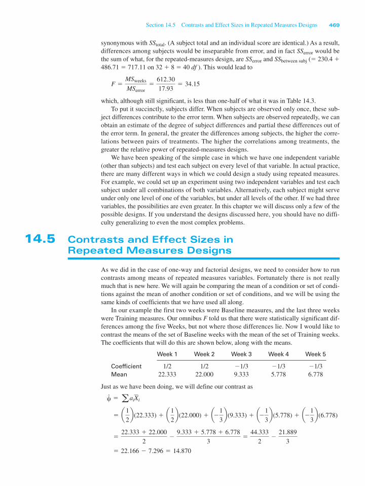
In our example the first two weeks were Baseline measures, and the last three weekswere Training measures. Our omnibus F told us that there were statistically significant dif-ferences among the five Weeks, but not where those differences lie. Now I would like tocontrast the means of the set of Baseline weeks with the mean of the set of Training weeks.The coefficients that will do this are shown below, along with the means.

Week 1 Week 2 Week 3 Week 4 Week 5

Coefficient 1/2 1/2 21/3 21/3 21/3Mean 22.333 22.000 9.333 5.778 6.778

Just as we have been doing, we will define our contrast as

= 22.166 2 7.296 = 14.870

= 22.333 1 22.0002

29.333 1 5.778 1 6.778

3= 44.333

22

21.8893

= a12b(22.333) 1 a1

2b(22.000) 1 a21

3b (9.333) 1 a21

3b(5.778) 1 a21

3b (6.778)

cN = aaiXi

F =MSweeks

MSerror= 612.30

17.93= 34.15

SSbetween subjSSerror

SSerror

SStotal

Section 14.5 Contrasts and Effect Sizes in Repeated Measures Designs 469

We can test this contrast with either a t or an F, but I will use t here. (F is just the square of t.)

This is a t on dferror 532 df, and is clearly statistically significant.Notice that in calculating my t, I used the MSerror from the overall analysis. And this

was the same error term that was used to test the Weeks effect. I point that out only becausewhen we come to more complex analyses we will have multiple error terms, and the one touse for a specific contrast is the one that was used to test the main effect of that independ-ent variable.

Effect Sizes

Although there was a direct translation from one-way designs to repeated measures designsin terms of testing contrasts among means, the situation is a bit more complicated when itcomes to estimating effect sizes. We will continue to define our effect size as

There should be no problem with , because it is the same contrast that we computedabove—the difference between the mean of the baseline weeks and the mean of the train-ing weeks. But there are several choices for serror. Kline (2004) gives 3 possible choicesfor our denominator, but points out that two of these are unsatisfactory either becausethey ignore the correlation between weeks or because they standardize by a standarddeviation that is not particularly meaningful. What we will actually do is create an errorterm that is unique to the particular contrast. We will form a contrast for each subject.That means that for each subject we will calculate the difference between his mean onthe baseline weeks and his mean on the training weeks. These are difference scores,which are analogous to the difference scores we computed for a paired sample t test. Thestandard deviation of these difference scores is analogous to the denominator we dis-cussed for computing effect size with paired data when we just had two repeated meas-ures with the t test. It is important to note that there is room for argument about theproper term to use to standardize contrasts with repeated measures. See Kline (2004) andOlejnik and Algina (2000).

For our migraine example the first subject would have a difference score of(21 1 22)/2 2 (8 1 6 1 6)/3 5 21.5 2 6.667 5 14.833. The complete set of differencescores would be

[14.833, 13.500, 11.333, 13.500, 19.500, 16.667, 17.000, 12.833, 14.667]

The mean of these difference scores is 14.879, which is . The standard deviation of thesedifference scores is 2.49. Then our effect size measure is

This tells us that the severity of headaches during baseline is nearly 6 standard devia-tions greater than the severity of head aches during training. That is a very large difference,and we can see that just by looking at the data. Remember, in calculating this effect sizewe have eliminated the variability between participants (subjects) in terms of headacheseverity. We are in a real sense comparing each individual to himself or herself.

dN =cN

serror= 14.87

2.49= 5.97.

cN

cN

cN

dN =cN

serror

t =cNB(aa2i )MSerror

n

= 14.870B0.833(7.20)9

= 14.87010.667= 14.870

0.816= 18.21


14.6 Writing Up the Results

In writing up the results of this experiment we could simply say:

To investigate the effects of relaxation therapy on the severity of migraine headaches,9 participants rated the severity of headaches on each of two weeks before receivingrelaxation therapy and for three weeks while receiving therapy. An overall analysisof variance for repeated measures showed a significant difference between weeks(F(4,32) 5 85.04, p , .05). The mean severity rating during baseline weeks was 22.166,which dropped to a mean of 7.296 during training, for a difference of 14.87. A contraston this difference was significant (t(32) 5 18.21, p , .05). Using the standard deviationof contrast differences for each participant produced an effect size measure of d 5 5.97,documenting the importance of relaxation therapy in treating migraine headaches.

14.7 One Between-Subjects Variable and One Within-Subjects Variable

Consider the data presented in Table 14.4. These are actual data from a study by King(1986). This study in some ways resembles the one on morphine tolerance by Siegel (1975)that we examined in Chapter 12. King investigated motor activity in rats following injectionof the drug midazolam. The first time that this drug is injected, it typically leads to a distinctdecrease in motor activity. Like morphine, however, a tolerance for midazolam developsrapidly. King wished to know whether that acquired tolerance could be explained on thebasis of a conditioned tolerance related to the physical context in which the drug was ad-ministered, as in Siegel’s work. He used three groups, collecting the crucial data (presentedin Table 14.4) on only the last day, which was the test day. During pretesting, two groups ofanimals were repeatedly injected with midazolam over several days, whereas the Controlgroup was injected with physiological saline. On the test day, one group—the “Same”group—was injected with midazolam in the same environment in which it had earlier beeninjected. The “Different” group was also injected with midazolam, but in a different envi-ronment. Finally, the Control group was injected with midazolam for the first time. ThisControl group should thus show the typical initial response to the drug (decreased ambula-tory behavior), whereas the Same group should show the normal tolerance effect—that is,they should decrease their activity little or not at all in response to the drug on the last trial.If King is correct, however, the Different group should respond similarly to the Controlgroup, because although they have had several exposures to the drug, they are receiving it ina novel context and any conditioned tolerance that might have developed will not have thenecessary cues required for its elicitation. The dependent variable in Table 14.4 is a measureof ambulatory behavior, in arbitrary units. Again, the first letter of the name of a variable isused as a subscript to indicate what set of means we are referring to.

Because the drug is known to be metabolized over a period of approximately 1 hour,King recorded his data in 5-minute blocks, or Intervals. We would expect to see the effectof the drug increase for the first few intervals and then slowly taper off. Our analysis usesthe first six blocks of data. The design of this study can then be represented diagrammati-cally as shown in next page.

Here we have distinguished those effects that represent differences between subjects fromthose that represent differences within subjects. When we consider the between-subjectsterm, we can partition it into differences between groups of subjects (G) and differencesbetween subjects in the same group (Ss w/in groups). The within-subject term can similarly

Section 14.7 One Between-Subjects Variable and One Within-Subjects Variable 471


Table 14.4 Ambulatory behavior by Group and Trial

(a) Data

Interval

1 2 3 4 5 6 Mean

Control 150 44 71 59 132 74 88.333335 270 156 160 118 230 211.500149 52 91 115 43 154 100.667159 31 127 212 71 224 137.333159 0 35 75 71 34 62.333292 125 184 246 225 170 207.000297 187 66 96 209 74 154.833170 37 42 66 114 81 85.000

Mean 213.875 93.250 96.500 128.625 122.875 130.125 130.875

Same 346 175 177 192 239 140 211.500426 329 236 76 102 232 233.500359 238 183 123 183 30 186.000272 60 82 85 101 98 116.333200 271 263 216 241 227 236.333366 291 263 144 220 180 244.000371 364 270 308 219 267 299.833497 402 294 216 284 255 324.667

Mean 354.625 266.250 221.000 170.000 198.625 178.625 231.521

Different 282 186 225 134 189 169 197.500317 31 85 120 131 205 148.167362 104 144 114 115 127 161.000338 132 91 77 108 169 152.500263 94 141 142 120 195 159.167138 38 16 95 39 55 63.500329 62 62 6 93 67 103.167

(continues)

Total variation

Between subjects

G(Groups)

Ss w/inGroups

Within subjects

I 3 Ss w/inGroups

I (Intervals)

I 3 G

be subdivided into three components—the main effect of Intervals (the repeated measure)and its interactions with the two partitions of the between-subject variation. You will see thispartitioning represented in the summary table when we come to it.

Partitioning the Between-Subjects Effects

Let us first consider the partition of the between-subjects term in more detail. From the de-sign of the experiment, we know that this term can be partitioned into two parts. One ofthese parts is the main effect of Groups (G), since the treatments (Control, Same, and Dif-ferent) involve different groups of subjects. This is not the only source of differencesamong subjects, however. We have eight different subjects within the control group, anddifferences among them are certainly between-subjects differences. The same holds for thesubjects within the other groups. Here we are speaking of differences among subjects inthe same group—that is, Ss within groups.


Table 14.4 (continued)

Interval

1 2 3 4 5 6 Mean

292 139 104 184 193 122 172.333

Mean 290.125 98.250 108.500 109.000 123.500 138.625 144.667

Interval 286.208 152.583 142.000 135.875 148.333 149.125 169.021mean

(b) Calculations

(c) Summary Table

Source df SS MS F

Between subjects 23 670,537.1Groups 2 285,815.0 142,907.5 7.80*Ss w/in groups** 21 384,722.0 18,320.1

Within subjects** 120 761,755.8Intervals 5 399,736.5 79,947.3 29.85*I 3 G 10 80,820.0 8,082.0 3.02*I 3 Ss w/in groups** 105 281,199.3 2,678.1

Total 143 1,432,292.9

* p , .05** Calculated by subtraction

SSI3G = SScells 2 SSinterval 2 SSgroups = 766,371.5 2 285,815.0 2 399.736.5 = 80,820.0

SScells = na (XGI 2 X...)2 = 83(213.875 2 169.021)2 1 Á 1 (138.625 2 169.021)24 = 766,371.5

SSintervals = nga (XI 2 X...)2 = 8 3 33(286.208 2 169.021)2 1 Á 1 (149.125 2 169.021)24 = 399,736.5

SSgroups = nia (XG 2 X...)2 = 8 3 63(130.875 2 169.021)2 1 Á 1 (144.667 2 169.021)24 = 285,815.0

SSsubj = ia (XS 2 X...)2 = 6[(88.333 2 169.021)2 1 Á 1 (172.333 2 169.021)2] = 670,537.1

SStotal = a (X 2 X...)2 = (150 2 169.021)2 1 Á 1 (122 2 169.021)2 = 1,432,292.9

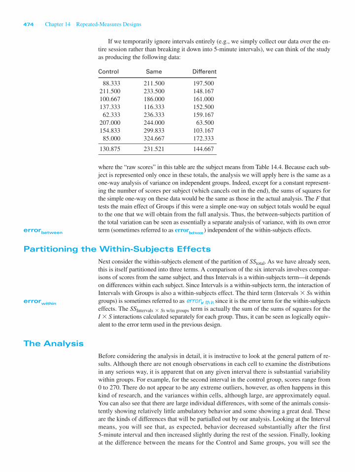
If we temporarily ignore intervals entirely (e.g., we simply collect our data over the en-tire session rather than breaking it down into 5-minute intervals), we can think of the studyas producing the following data:


Control Same Different

88.333 211.500 197.500211.500 233.500 148.167100.667 186.000 161.000137.333 116.333 152.50062.333 236.333 159.167

207.000 244.000 63.500154.833 299.833 103.16785.000 324.667 172.333

130.875 231.521 144.667

where the “raw scores” in this table are the subject means from Table 14.4. Because each sub-ject is represented only once in these totals, the analysis we will apply here is the same as aone-way analysis of variance on independent groups. Indeed, except for a constant represent-ing the number of scores per subject (which cancels out in the end), the sums of squares forthe simple one-way on these data would be the same as those in the actual analysis. The F thattests the main effect of Groups if this were a simple one-way on subject totals would be equalto the one that we will obtain from the full analysis. Thus, the between-subjects partition ofthe total variation can be seen as essentially a separate analysis of variance, with its own errorterm (sometimes referred to as errorbetween) independent of the within-subjects effects.

Partitioning the Within-Subjects Effects

Next consider the within-subjects element of the partition of . As we have already seen,this is itself partitioned into three terms. A comparison of the six intervals involves compar-isons of scores from the same subject, and thus Intervals is a within-subjects term—it dependson differences within each subject. Since Intervals is a within-subjects term, the interaction ofIntervals with Groups is also a within-subjects effect. The third term (Intervals 3 Ss withingroups) is sometimes referred to as since it is the error term for the within-subjectseffects. The term is actually the sum of the sums of squares for theI 3 S interactions calculated separately for each group. Thus, it can be seen as logically equiv-alent to the error term used in the previous design.

The Analysis

Before considering the analysis in detail, it is instructive to look at the general pattern of re-sults. Although there are not enough observations in each cell to examine the distributionsin any serious way, it is apparent that on any given interval there is substantial variabilitywithin groups. For example, for the second interval in the control group, scores range from0 to 270. There do not appear to be any extreme outliers, however, as often happens in thiskind of research, and the variances within cells, although large, are approximately equal.You can also see that there are large individual differences, with some of the animals consis-tently showing relatively little ambulatory behavior and some showing a great deal. Theseare the kinds of differences that will be partialled out by our analysis. Looking at the Intervalmeans, you will see that, as expected, behavior decreased substantially after the first 5-minute interval and then increased slightly during the rest of the session. Finally, lookingat the difference between the means for the Control and Same groups, you will see the

SSIntervals 3 Ss w/in groups

errorwithin

SStotal

errorbetween

errorwithin

anticipated tolerance effect, and looking at the Different group, you see that it is much morelike the Control group than it is like the Same group. This is the result that King predicted.

Very little needs to be said about the actual calculations in Table 14.4b, since they arereally no different from the usual calculations of main and interaction effects. Whether afactor is a between-subjects or within-subjects factor has no bearing on the calculation ofits sum of squares, although it does affect its placement in the summary table and the ulti-mate calculation of the corresponding F.

In the summary table in Table 14.4c, the source column reflects the design of the ex-periment, with first partitioned into and . Each of these sumsof squares is further subdivided. The double asterisks next to the three terms show we cal-culate these by subtraction ( , , and ), based on thefact that sums of squares are additive and the whole must be equal to the sum of its parts.This simplifies our work considerably. Thus

These last two terms will become error terms for the analysis.The degrees of freedom are obtained in a relatively straightforward manner. For each

of the main effects, the number of degrees of freedom is equal to the number of levelsof the variable minus 1. Thus, for Subjects there are 24 2 1 5 23 df, for Groups there are3 2 1 5 2 df, and for Intervals there are 6 2 1 5 5 df. As for all interactions, the df for I 3 Gis equal to the product of the df for the component terms. Thus, .The easiest way to obtain the remaining degrees of freedom is by subtraction, just as wedid with the corresponding sums of squares.

These df can also be obtained directly by considering what these terms represent. Withineach subject, we have 6 2 1 5 5 df. With 24 subjects, this amounts to Within each level of the Groups factor, we have 8 2 1 5 7 df between subjects, and with threeGroups we have . I 3 Ss w/in groups is really an interaction term, andas such its df is simply the product of and .

Skipping over the mean squares, which are merely the sums of squares divided by theirdegrees of freedom, we come to F. From the column of F it is apparent that, as we anticipated,Groups and Intervals are significant. The interaction is also significant, reflecting, in part, thefact that the Different group was at first intermediate between the Same and the Control group,but that by the second 5-minute interval it had come down to be equal to the Control group.This finding can be explained by a theory of conditioned tolerance. The really interesting find-ing is that, at least for the later intervals, simply injecting an animal in an environment differentfrom the one in which it had been receiving the drug was sufficient to overcome the tolerancethat had developed. These animals respond almost exactly as do animals that had never experi-enced midazolam. We will return to the comparison of Groups at individual Intervals later.

Assumptions

For the F ratios actually to follow the F distribution, we must invoke the usual assumptionsof normality, homogeneity of variance, and sphericity of . For the between-subjects term(s),this means that we must assume that the variance of subject means within any one level of

gN

(5)(21) = 105dfSs w/in groups 5dfI(7)(3) = 21 dfw/in groups

120 dfw/in subj.(5)(24) 5

dfI3Ss w/in groups = dfw/in subj 2 dfintervals 2 dfIG

dfSs w/in groups = dfbetween subj 2 dfgroups

dfw/in subj = dftotal 2 dfbetween subj

dfIG = (6–1)(3–1) = 10

SSI3Ss w/in groups = SSw/in subj 2 SSintervals 2 SSIG

SSSs w/in groups = SSbetween subj 2 SSgroups

SSw/in subj = SStotal 2 SSbetween subj

SSI3Ss w/in groupsSSSs w/in groupsSSw/in subj

SSw/in subjSSbetween subjSStotal


Group is the same as the variance of subject means within every other level of Group. Ifnecessary, this assumption can be tested by calculating each of the variances and testing using either or, preferably, the test proposed by Levene (1960) orO’Brien (1981), which were referred to in Chapter 7. In practice, however, the analysis ofvariance is relatively robust against reasonable violations of this assumption (see Collier,Baker, and Mandeville, 1967; and Collier, Baker, Mandeville, and Hayes, 1967). Because thegroups are independent, compound symmetry, and thus sphericity, of the covariance matrix isassured if we have homogeneity of variance, since all off-diagonal entries will be zero.

For the within-subjects terms we must also consider the usual assumptions of homo-geneity of variance and normality. The homogeneity of variance assumption in this case isthat the I 3 S interactions are constant across the Groups, and here again this can be testedusing . (You would simply calculate an I 3 S interactionfor each group—equivalent to the error term in Table 14.3—and test the largest against thesmallest.) For the within-subjects effects, we must also make assumptions concerning thecovariance matrix.

There are two assumptions on the covariance matrix (or matrices). Again, we will letrepresent the matrix of variances and covariances among the levels of I (Intervals). Thus

with six intervals,

I1 I2 I3 I4 I5 I6

5

For each Group we would have a separate population variance-covariance matrix .( and are estimated by and , respectively.) For to be an appro-priate error term, we will first assume that the individual variance–covariance matrices ( )are the same for all levels of G. This can be thought of as an extension (to covariances) ofthe common assumption of homogeneity of variance.

The second assumption concerning covariances deals with the overall matrix , whereis the pooled average of the . (For equal sample sizes in each group, an entry in will

be the average of the corresponding entries in the individual matrices.) A common andsufficient, but not necessary, assumption is that the matrix exhibits compound symmetry—meaning, as I said earlier, that all the variances on the main diagonal are equal, and all the co-variances off the main diagonal are equal. Again, the variances do not have to equal thecovariances, and usually will not. This assumption is in fact more stringent than necessary.All that we really need to assume is that the standard errors of the differences between pairsof Interval means are constant—in other words, that is constant for all i and j ( j i).

This sphericity requirement is met automatically if exhibits compound symmetry, but otherpatterns of will also have this property. For a more extensive discussion of the covarianceassumptions, see Huynh and Feldt (1970) and Huynh and Mandeville (1979); a particularlygood discussion can be found in Edwards (1985, pp. 327–329, 336–339).

Adjusting the Degrees of Freedom

Box (1954a) and Greenhouse and Geisser (1959) considered the effects of departure from thissphericity assumption on . They showed that regardless of the form of , the F ratio from thegg

g g±sIi2Ij

2

gGi

ggGig g

gGi

MSI3Ss w/in groupsgN GigNgGiggGi

sN 66sN 65sN 64sN 63sN 62sN 61



sN 36sN 35sN 34sN 33sN 32sN 31gNsN 26sN 25sN 24sN 23sN 22sN 21


gN

Fmax on g and (n 2 1)(i 2 1)df

Fmax on (g, n 2 1)df


within-subjects portion of the analysis of variance will be approximately distributed as F on

(i 2 1) , g(n 2 1)(i 2 1)

df for the Interval effect and

(g 2 1)(i 2 1) , g(n 2 1)(i 2 1)

df for the I 3 G interaction, where i 5 the number of intervals and is estimated by

Here,

the mean of the entries on the main diagonal of

the mean of all entries in the jkth entry in

the mean of all entries in the jth row of

The effect of using is to decrease both and from what they would nor-mally be. Thus is simply the proportion by which we reduce them. Greenhouse andGeisser recommended that we adjust our degrees of freedom using . They further showedthat when the sphericity assumptions are met, 5 1, and as we depart more and more fromsphericity, approaches 1/(i 2 1) as a minimum.

There is some suggestion that for large values of , even using to adjust the degrees offreedom can lead to a conservative test. Huynh and Feldt (1976) investigated this correctionand recommended a modification of when there is reason to believe that the true value of

lies near or above 0.75. Huynh and Feldt, as later corrected by Lecoutre (1991), defined

where N 5 n 3 g. (Chen and Dunlap [1994] later confirmed Lecoutre’s correction tothe original Huynh and Feldt formula.3) We then use or , depending on our estimateof the true value of . (Under certain circumstances, will exceed 1, at which point it isset to 1.)

A test on the assumption of sphericity has been developed by Mauchly (1940) and eval-uated by Huynh and Mandeville (1979) and by Keselman, Rogan, Mendoza, and Breen(1980), who point to its extreme lack of robustness. This test is available on SPSS, SAS,and other software, and is routinely printed out. Because tests of sphericity are likely tohave serious problems when we need them the most, it has been suggested that we alwaysuse the correction to our degrees of freedom afforded by or , whichever is appropriate,or use a multivariate procedure to be discussed later. This is a reasonable suggestion andone worth adopting.

For our data, the F value for Intervals (F 5 29.85) is such that its interpretation wouldbe the same regardless of the value of , since the Interval effect will be significant evenfor the lowest possible df. If the assumption of sphericity is found to be invalid, however,alternative treatments would lead to different conclusions with respect to the I 3 G interac-tion. For King’s data, the Mauchly’s sphericity test, as found from SPSS, indicates that theassumption has been violated, and therefore it is necessary to deal with the problem resultingfrom this violation.

´

~́Ń

~́´

~́Ń

~́ =(N 2 g 1 1)(i 2 1)Ń 2 2

(i 2 1)[N 2 g 2 (i 2 1)Ń ]

´Ń

Ń´´

´Ń

ŃdferrordfeffectŃ

gNsj =gNsjk =

gNs =gNsjj =

Ń =i2(sjj 2 s)2

(i 2 1)Aa s2jk 2 2ia s2

j 1 i2s2B´

´´

´´


3 Both SPSS and SAS continue to calculate the wrong value for the Huynh and Feldt epsilon.

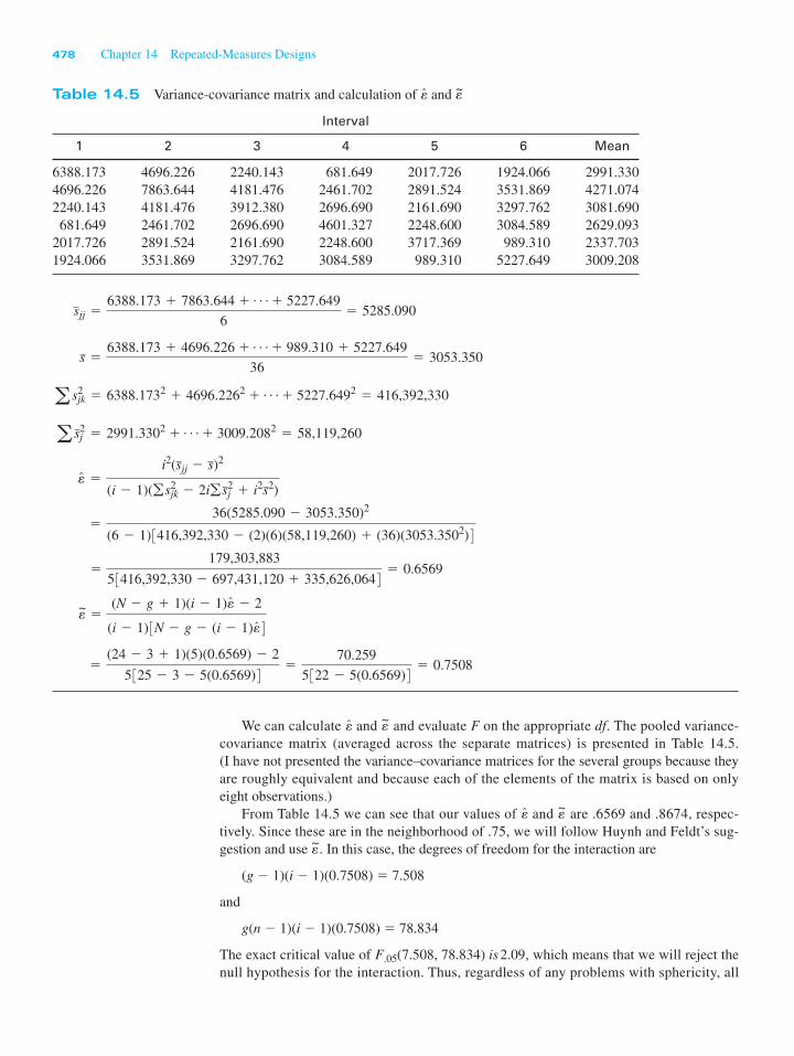
We can calculate and and evaluate F on the appropriate df. The pooled variance-covariance matrix (averaged across the separate matrices) is presented in Table 14.5. (I have not presented the variance–covariance matrices for the several groups because theyare roughly equivalent and because each of the elements of the matrix is based on onlyeight observations.)

From Table 14.5 we can see that our values of and are .6569 and .8674, respec-tively. Since these are in the neighborhood of .75, we will follow Huynh and Feldt’s sug-gestion and use . In this case, the degrees of freedom for the interaction are

(g 2 1)(i 2 1)(0.7508) 5 7.508

and

g(n 2 1)(i 2 1)(0.7508) 5 78.834

The exact critical value of , which means that we will reject thenull hypothesis for the interaction. Thus, regardless of any problems with sphericity, all

F.05(7.508, 78.834) is2.09

~́

~́Ń

~́Ń


Table 14.5 Variance-covariance matrix and calculation of and

Interval

1 2 3 4 5 6 Mean

6388.173 4696.226 2240.143 681.649 2017.726 1924.066 2991.3304696.226 7863.644 4181.476 2461.702 2891.524 3531.869 4271.0742240.143 4181.476 3912.380 2696.690 2161.690 3297.762 3081.690681.649 2461.702 2696.690 4601.327 2248.600 3084.589 2629.093

2017.726 2891.524 2161.690 2248.600 3717.369 989.310 2337.7031924.066 3531.869 3297.762 3084.589 989.310 5227.649 3009.208

=(24 2 3 1 1)(5)(0.6569) 2 2

5325 2 3 2 5(0.6569)4 = 70.2595322 2 5(0.6569)4 = 0.7508

~́ =(N 2 g 1 1)(i 2 1)Ń 2 2

(i 2 1)3N 2 g 2 (i 2 1)Ń 4=

179,303,88353416,392,330 2 697,431,120 1 335,626,0644 = 0.6569

=36(5285.090 2 3053.350)2

(6 2 1)3416,392,330 2 (2)(6)(58,119,260) 1 (36)(3053.3502)4Ń =

i2(sjj 2 s)2

(i 2 1)(gs2jk 2 2igs2

j 1 i2s2)

a s2j = 2991.3302 1 Á 1 3009.2082 = 58,119,260

a s2jk = 6388.1732 1 4696.2262 1 Á 1 5227.6492 = 416,392,330

s = 6388.173 1 4696.226 1 Á 1 989.310 1 5227.64936

= 3053.350

sjj = 6388.173 1 7863.644 1 Á 1 5227.6496

= 5285.090

~́Ń


the effects in this analysis are significant. (They would also be significant if we used instead of .)

Simple Effects

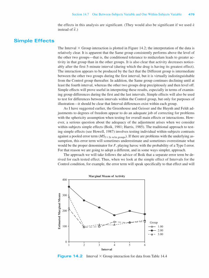
The Interval 3 Group interaction is plotted in Figure 14.2; the interpretation of the data isrelatively clear. It is apparent that the Same group consistently performs above the level ofthe other two groups—that is, the conditioned tolerance to midazolam leads to greater ac-tivity in that group than in the other groups. It is also clear that activity decreases notice-ably after the first 5-minute interval (during which the drug is having its greatest effect).The interaction appears to be produced by the fact that the Different group is intermediatebetween the other two groups during the first interval, but it is virtually indistinguishablefrom the Control group thereafter. In addition, the Same group continues declining until atleast the fourth interval, whereas the other two groups drop precipitously and then level off.Simple effects will prove useful in interpreting these results, especially in terms of examin-ing group differences during the first and the last intervals. Simple effects will also be usedto test for differences between intervals within the Control group, but only for purposes ofillustration—it should be clear that Interval differences exist within each group.

As I have suggested earlier, the Greenhouse and Geisser and the Huynh and Feldt ad-justments to degrees of freedom appear to do an adequate job of correcting for problemswith the sphericity assumption when testing for overall main effects or interactions. How-ever, a serious question about the adequacy of the adjustment arises when we considerwithin-subjects simple effects (Boik, 1981; Harris, 1985). The traditional approach to test-ing simple effects (see Howell, 1987) involves testing individual within-subjects contrastsagainst a pooled error term ( ). If there are problems with the underlying as-sumption, this error term will sometimes underestimate and sometimes overestimate whatwould be the proper denominator for F, playing havoc with the probability of a Type I error.For that reason we are going to adopt a different, and in some ways simpler, approach.

The approach we will take follows the advice of Boik that a separate error term be de-rived for each tested effect. Thus, when we look at the simple effect of Intervals for theControl condition, for example, the error term will speak specifically to that effect and will

MSI3Ss w/in groups

~́Ń

Marginal Means of Activity

Interval654321

Est

imat

ed M

argi

nal M

eans

400

300

200

100

0

Group1.002.003.00

Figure 14.2 Interval 3 Group interaction for data from Table 14.4

not pool other error terms that apply to other simple effects. In other words, it will be basedsolely on the Control group. We can test the Interval simple effects quite easily by runningseparate repeated-measures analyses of variance for each of the groups. For example, wecan run a one-way repeated-measures analysis on Intervals for the Control group, as dis-cussed in Section 14.4. We can then turn around and perform similar analyses on Intervalsfor the Same and Different groups separately. These results are shown in Table 14.6. Ineach case the Interval differences are significant, even after we correct the degrees of free-dom using or , whichever is appropriate.

If you look at the within-subject analyses in Table 14.6, you will see that the averageis (2685.669 1 3477.571 1 1871.026)/3 5 2678.089, which is

from the overall analysis found on page 473. Here these denominators for the F ratios arenoticeably different from what they would have been had we used the pooled term, whichis the traditional approach. You can also verify with a little work that the termsfor each analysis are the same as those that we would compute if we followed the usualprocedures for obtaining simple effects mean squares.

For the between-subjects simple effects (e.g., Groups at Interval 1) the procedure ismore complicated. Although we could follow the within-subject example and perform sep-arate analyses at each Interval, we would lose considerable degrees of freedom unnecessarily.Here it is usually legitimate to pool error terms, and it is generally wise to do so.

MSInterval

MSI3Ss w/in groupsMSerror

~́Ń


Table 14.6 Calculation of within-subjects simple effects for data from King (1986)

(a) Interval at Control

Source df SS MS F

Between subjects 7 134,615.58Interval 5 76,447.25 15,289.45 5.69*Error 35 93,998.42 2685.67

Total 47 305,061.25

*p , .05; 5 .404; 5 .570

(b) Interval at Same

Source df SS MS F


Total 47 490,405.98

*p , .05; 5 .578; 5 1.00

(c) Interval at Different

Source df SS MS F


Total 47 351,010.67

*p , .05; 5 .598; 5 1.00~́Ń

~́Ń

~́Ń

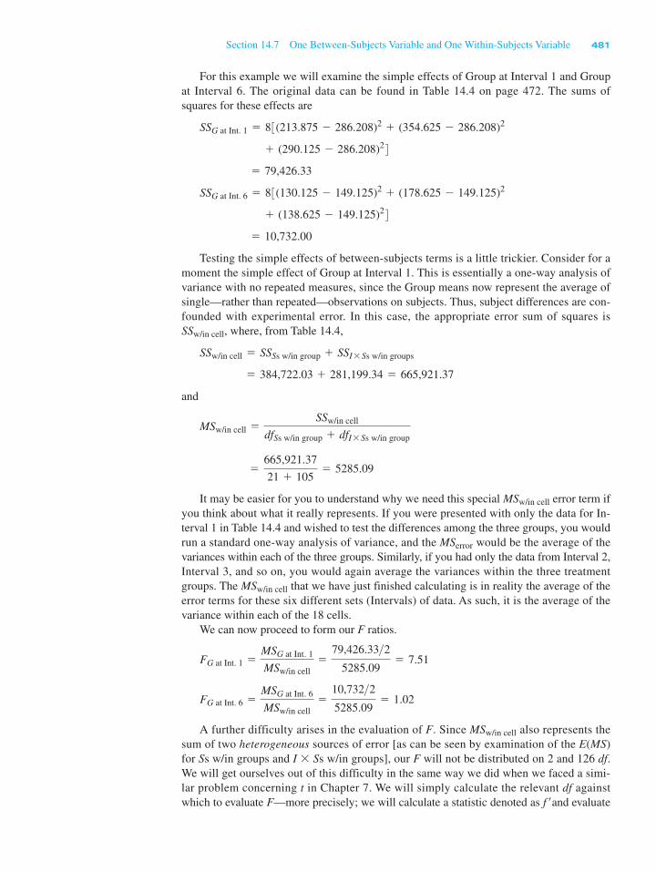
For this example we will examine the simple effects of Group at Interval 1 and Groupat Interval 6. The original data can be found in Table 14.4 on page 472. The sums ofsquares for these effects are

Testing the simple effects of between-subjects terms is a little trickier. Consider for amoment the simple effect of Group at Interval 1. This is essentially a one-way analysis ofvariance with no repeated measures, since the Group means now represent the average ofsingle—rather than repeated—observations on subjects. Thus, subject differences are con-founded with experimental error. In this case, the appropriate error sum of squares is

, where, from Table 14.4,

and

It may be easier for you to understand why we need this special error term ifyou think about what it really represents. If you were presented with only the data for In-terval 1 in Table 14.4 and wished to test the differences among the three groups, you wouldrun a standard one-way analysis of variance, and the would be the average of thevariances within each of the three groups. Similarly, if you had only the data from Interval 2,Interval 3, and so on, you would again average the variances within the three treatmentgroups. The that we have just finished calculating is in reality the average of theerror terms for these six different sets (Intervals) of data. As such, it is the average of thevariance within each of the 18 cells.

We can now proceed to form our F ratios.

A further difficulty arises in the evaluation of F. Since also represents thesum of two heterogeneous sources of error [as can be seen by examination of the E(MS)for Ss w/in groups and I 3 Ss w/in groups], our F will not be distributed on 2 and 126 df.We will get ourselves out of this difficulty in the same way we did when we faced a simi-lar problem concerning t in Chapter 7. We will simply calculate the relevant df againstwhich to evaluate F—more precisely; we will calculate a statistic denoted as and evaluatef ¿

MSw/in cell

FG at Int. 6 =MSG at Int. 6

MSw/in cell=

10,732>25285.09

= 1.02

FG at Int. 1 =MSG at Int. 1

MSw/in cell=

79,426.33>25285.09

= 7.51

MSw/in cell

MSerror

MSw/in cell

=665,921.3721 1 105

= 5285.09

MSw/in cell =SSw/in cell

dfSs w/in group 1 dfI3Ss w/in group

= 384,722.03 1 281,199.34 = 665,921.37

SSw/in cell = SSSs w/in group 1 SSI3Ss w/in groups

SSw/in cell

= 10,732.00

1 (138.625 2 149.125)24SSG at Int. 6 = 83(130.125 2 149.125)2 1 (178.625 2 149.125)2

= 79,426.33

1 (290.125 2 286.208)24SSG at Int. 1 = 83(213.875 2 286.208)2 1 (354.625 2 286.208)2


against . In this case, the value of is given by Welch (1938) andSatterthwaite (1946) as

where

and are the corresponding degrees of freedom. For our example,

Rounding to the nearest integer gives 5 57. Thus, our F is distributed on (g 2 1, ) 5(2, 57) df under . For 2 and 57 df, F.05 5 3.16. Only the difference at Interval 1 is signif-icant. By the end of 30 minutes, the three groups were performing at equivalent levels. It islogical to conclude that somewhere between the first and the sixth interval the three groupsbecome nonsignificantly different, and many people test at each interval to find that point.However, I strongly recommend against this practice as a general rule. We have already runa number of significance tests, and running more of them serves only to increase the errorrate. Unless there is an important theoretical reason to determine the point at which thegroup differences become nonsignificant—and I suspect that there are very few suchcases—then there is nothing to be gained by testing each interval. Tests should be carriedout to answer important questions, not to address idle curiosity or to make the analysis look“complete.”

Multiple Comparisons

Several studies have investigated the robustness of multiple-comparison procedures fortesting differences among means on the within-subjects variable. Maxwell (1980) studied asimple repeated-measures design with no between-subject component and advised adopt-ing multiple-comparison procedures that do not use a pooled error term. We discussed sucha procedure (the Games-Howell procedure) in Chapter 12. (I did use a pooled error term inthe analysis of the migraine study, but there it was reasonable to assume homogeneity ofvariance and I was using all of the weeks. If I had only been running a contrast involvingthree of the weeks, I would seriously consider calculating an error term based on just thedata from those weeks.)

Keselman and Keselman (1988) extended Maxwell’s work to designs having one be-tween-subject component and made a similar recommendation. In fact, they showed thatwhen the Groups are of different sizes and sphericity is violated, familywise error rates canbecome very badly distorted. In the simple effects procedures that we have just considered,I recommended using separate error terms by running one-way repeated-measures analy-ses for each of the groups. For subsequent multiple-comparison procedures exploring thosesimple effects, especially with unequal sample sizes, it would probably be wise to employ

H0

f ¿f ¿

f ¿ =(384,722.03 1 281,199.34)2

384,722.032

211

281,199.342

105

= 56.84

dfv = 105v = 281,199.34

dfu = 21u = 384,722.03

dfu and dfv

v = SSI3Ss w/in groups

u = SSSs w/in groups

f ¿ =(u 1 v)2

u2

dfu1

v2

dfv

f ¿F.05(a 2 1, f ¿)Fobt


the Games-Howell procedure using those separate covariance matrices. In other words, tocompare Intervals 3 and 4 for the Control group, you would generate your error term usingonly the Intervals 3 and 4 data from just the Control group.

Myers (1979) has suggested making post hoc tests on a repeated measure using pairedt-tests and a Bonferroni correction. (This is essentially what I did for the migraine exam-ple, though a Bonferroni correction was not necessary because I ran only one contrast.)Maxwell (1980) showed that this approach does a good job of controlling the familywiseerror rate, and Baker and Lew (1987) showed that it generally compared well againstTukey’s test in terms of power. Baker proposed a simple modification of the Bonferroni(roughly in line with that of Holm) that had even greater power.

14.8 Two Between-Subjects Variables and One Within-Subjects Variable

The basic theory of repeated-measures analysis of variance has already been described inthe discussion of the previous designs. However, experimenters commonly plan experi-ments with three or more variables, some or all of which represent repeated measures onthe same subjects. We will briefly discuss the analysis of these designs. The calculationsare straight forward, because the sums of squares for main effects and interactions are ob-tained in the usual way and the error terms are obtained by subtraction.

We will not consider the theory behind these designs at any length. Essentially, itamounts to the extrapolation of what has already been said about the two-variable case. Foran excellent discussion of the underlying statistical theory see Winer (1971) or Maxwelland Delaney (2004).

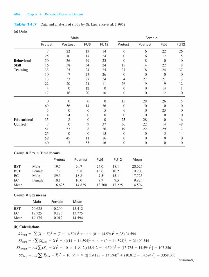
I will take as an example a study by St. Lawrence, Brasfield, Shirley, Jefferson, Alleyne,and O’Bannon (1995) on an intervention program to reduce the risk of HIV infection amongAfrican-American adolescents. The study involved a comparison of two approaches, one ofwhich was a standard 2-hour educational program used as a control condition (EC) and theother was an 8-week behavioral skills training program (BST). Subjects were Male andFemale adolescents, and measures were taken at Pretest, Posttest, and 6 and 12 monthsfollow-up (FU6 and FU12). There were multiple dependent variables in the study, but theone that we will consider is log(freq 1 1), where freq is the frequency of condom-protectedintercourse.4 This is a 2 3 2 3 4 repeated-measures design, with Intervention and Sex asbetween-subjects factors and Time as the within-subjects factor. This design may be dia-grammed as follows, where represents the ith group of subjects.

Behavioral Skills Training Educational Control

Pretest Posttest FU6 FU12 Pretest Posttest FU6 FU12

MaleFemale

The raw data and the necessary summary tables of cell totals are presented in Table 14.7a.(These data have been generated to closely mimic the data reported by St. Lawrence et al.,though they had many more subjects. Decimal points have been omitted.) In Table 14.7b arethe calculations for the main effects and interactions. Here, as elsewhere, the calculations arecarried out exactly as they are for any main effects and interactions.

G4G4G4G4G3G3G3G3

G2G2G2G2G1G1G1G1

Gi

Section 14.8 Two Between-Subjects Variables and One Within-Subjects Variable 483

4 The authors used a logarithmic transformation here because the original data were very positively skewed. Theytook the log of (X 1 1) instead of X because log(0) is not defined.


Table 14.7 Data and analysis of study by St. Lawrence et al. (1995)

(a) Data

Male Female

Pretest Posttest FU6 FU12 Pretest Posttest FU6 FU12

7 22 13 14 0 6 22 2625 10 17 24 0 16 12 15

Behavioral 50 36 49 23 0 8 0 0Skill 16 38 34 24 15 14 22 8Training 33 25 24 25 27 18 24 37

10 7 23 26 0 0 0 013 33 27 24 4 27 21 322 20 21 11 26 9 9 124 0 12 0 0 0 14 1

17 16 20 10 0 0 12 0

0 0 0 0 15 28 26 1569 56 14 36 0 0 0 05 0 0 5 6 0 23 04 24 0 0 0 0 0 0

Educational 35 8 0 0 25 28 0 16Control 7 0 9 37 36 22 14 48

51 53 8 26 19 22 29 225 0 0 15 0 0 5 1459 45 11 16 0 0 0 040 2 33 16 0 0 0 0

Group 3 Sex 3 Time means

Pretest Posttest FU6 FU12 Mean

BST Male 19.7 20.7 24.0 18.1 20.625BST Female 7.2 9.8 13.6 10.2 10.200EC Male 29.5 18.8 7.5 15.1 17.725EC Female 10.1 10.0 9.7 9.5 9.825Mean 16.625 14.825 13.700 13.225 14.594

Group 3 Sex means

Male Female Mean

BST 20.625 10.200 15.412EC 17.725 9.825 13.775Mean 19.175 10.012 14.594

(b) Calculations

SSSex = ntga (XSex 2 X )2 = 10 3 4 3 23(19.175 2 14.594)2 1 (10.012 2 14.594)24 = 3358.056

SSgroup = ntsa (XG 2 X )2 = 10 3 4 3 23(15.412 2 14.594)2 1 (13.775 2 14.594)24 = 107.256

SSsubj = ta (XSubj 2 X )2 = 43(14 2 14.594)2 1 Á 1 (0 2 14.594)24 = 21490.344

SStotal = a (X 2 X )2 = (7 2 14.594)2 1 Á 1 (0 2 14.594)2 = 35404.594

(continues)


Table 14.7 (continued)

(c) Summary Table

Source df SS MS F

Between subjects 39 21,490.344Group (Condition) 1 107.256 107.256 0.21Sex 1 3358.056 3358.056 6.73*G 3 S 1 63.757 63.757 0.13Ss win groups** 36 17,961.275 498.924

Within subjects** 120 13,914.250Time 3 274.069 91.356 0.90T 3 G 3 1377.819 459.273 4.51*T 3 S 3 779.919 259.973 2.55T 3 G 3 S 3 476.419 158.806 1.56T 3 Ss w/in groups** 108 11,006.025 101.908

Total 159 35,404.594

*p , .05** Obtained by subtraction

= 6437.294 2 107.256 2 274.069 2 3358.056 2 1377.819 2 63.757 2 779.919 = 476.419

SSGTS = SScells GTS 2 SSG 2 SST 2 SSS 2 SSGT 2 SSGS 2 SSTS

SScells GTS = na (Xcells GTS 2 X )2 = 103(19.7–14.594)2 1 Á 1 (9.50–14.594)24 = 6437.294

SSTS = SScells TS 2 SST 2 SSS = 4412.044 2 274.069 2 3358.056 = 779.919

SScells TS = nga (Xcells TS 2 X )2 = 10 3 23(24.60 2 14.594)2 1 Á 1 (9.85 2 14.594)24 = 4412.044

SSTG = SScells TG 2 SST 2 SSG = 1759.144 2 274.069 2 107.256 = 1377.819

SScells TG = nsa (Xcells TG 2 X )2 = 10 3 23(13.45 2 14.594)2 1 Á 1 (12.300 2 14.594)24 = 1759.144

SStime = ngsa (XT 2 X )2 = 10 3 2 3 23(16.625 2 14.594)2 1 Á 1 (13.225 2 14.594)24 = 274.069

SSGS = SScells GS 2 SSG 2 SSS = 3529.069 2 107.256 2 3358.056 = 63.757

SScells GS = nta (Xcells GS 2 X )2 = 10 3 43(20.625 2 14.594)2 1 Á 1 (9.825 2 14.594)24 = 3529.069

The summary table for the analysis of variance is presented in Table 14.7c. In this table,the ** indicate terms that were obtained by subtraction. Specifically,

These last two terms are the error terms for between-subjects and within-subjects effects,respectively. That these error terms are appropriate is shown by examining the expectedmean squares presented in Table 14.8 on page 486.5 For the expected mean squares of ran-dom and mixed models, see Kirk (1968) or Winer (1971).

SST3Ss w/in groups = SSw/in subj 2 SST 2 SSTG 2 SSTS 2 SSTGS

SSSs w/in groups = SSbetween subj 2 SSG 2 SSS 2 SSGS

SSw/in subj = SStotal 2 SSbetween subj

5 As in earlier tables of expected mean squares, we use the to refer to the variance of random terms and torefer to the variability of fixed terms. Subjects are always treated as random, whereas in this study the two mainindependent variables are fixed.

u2s2

From the column of F in the summary table of Table 14.7c, we see that the main effect ofSex is significant, as is the Time 3 Group interaction. Both of these results are meaningful.As you will recall, the dependent variable is a measure of the frequency of use of condoms(log(freq 1 1)). Examination of the means reveals adolescent girls report a lower frequencyof use than adolescent boys. That could mean either that they have a lower frequency of in-tercourse, or that they use condoms a lower percentage of the time. Supplementary datasupplied by St. Lawrence et al. show that females do report using condoms a lower percent-age of the time than males, but not enough to account for the difference that we see here.Apparently what we are seeing is a reflection of the reported frequency of intercourse.

The most important result in this summary table is the Time 3 Group interaction. Thisis precisely what we would be looking for. We don’t really care about a Group effect, be-cause we would like the groups to be equal at pretest, and that equality would dilute anyoverall group difference. Nor do we particularly care about a main effect of Time, becausewe expect the Control group not to show appreciable change over time, and that woulddilute any Time effect. What we really want to see is that the BST group increases their useover time, whereas the EC group remains constant. That is an interaction, and that is whatwe found.

Simple Effects for Complex Repeated-Measures Designs

In the previous example we saw that tests on within-subjects effects were occasionally dis-rupted by violations of the sphericity assumption, and we took steps to work around thisproblem. We will have much the same problem with this example.

The cell means plotted in Figure 14.3 reveal the way in which frequency of condomuse changes over time for the two treatment conditions and for males and females sepa-rately. It is clear from this figure that the data do not tell a simple story.

We are again going to have to distinguish between simple effects on between-subjectfactors and simple effects on within-subject factors. We will start with between-subjectsimple effects. We have three different between-subjects simple effects that we couldexamine—namely: the simple main effects of Condition and Sex at each Time, and theSex 3 Condition simple interaction effect at each Time. For example, we might wish tocheck that the two Conditions (BST and EC) do not differ at pretest. Again, we might alsowant to test that they do differ at FU6 and/or at FU12. Here we are really dissecting theCondition 3 Time interaction effect, which we know from Table 14.7 to be significant.


Table 14.8 Expected mean squares with A, B, and C fixed

Source df SS

Between subjects abn 2 1A a 2 1B b 2 1AB (a 2 1)(b 2 1)Ss w/in groups ab(n 2 1)

Within subjects abn(c 2 1)C c 2 1AC (a 2 1)(c 2 1)BC (b 2 1)(c 2 1)ABC (a 2 1) (b 2 1)(c 2 1)C 3 Ss w/in groups ab(n 2 1)(c 2 1)

Total N 2 1

s2e 1 s2

gp

s2e 1 s2

gp 1 nu2abg

s2e 1 s2

gp 1 nau2bg

s2e 1 s2

gp 1 nbu2ag

s2e 1 s2

gp 1 nabu2g

s2e 1 cs2

p

s2e 1 cs2

p 1 ncu2ab

s2e 1 cs2

p 1 nacu2b

s2e 1 cs2

p 1 nbcu2a

By far the easiest way to test these between-subjects effects is to run separate two-way(Condition 3 Sex) analyses at each level of the Time variable. These four analyses willgive you all three simple effects at each Time with only minor effort. You can then acceptthe F values from these analyses, as I have done here for convenience, or you can pool theerror terms from the four separate analyses and use that pooled error term in testing themean square for the relevant effect. If these terms are heterogeneous, you would be wisenot to pool them. On the other hand, if they represent homogeneous sources of variance,they may be pooled, giving you more degrees of freedom for error. For these effects youdon’t need to worry about sphericity because each simple effect is calculated on only onelevel of the repeated-measures variable.

The within-subjects simple effects are handled in much the same way. For example,there is some reason to look at the simple effects of Time for each Condition separately tosee whether the EC condition shows changes over time in the absence of a complete inter-vention. Similarly, we would like to see how the BST condition changes with time. How-ever, we want to include Sex as an effect in both of these analyses so as not to inflate theerror term unnecessarily. We also want to use a separate error term for each analysis, ratherthan pooling these across Conditions.

The relevant analyses are presented in Table 14.9 for simple effects at one level of theother variable. Tests at the other levels would be carried out in the same way. Although thistable has more simple effects than we care about, they are presented to illustrate the way inwhich tests were constructed. You would probably be foolish to consider all of the tests thatresult from this approach, because you would seriously inflate the familywise error rate.Decide what you want to look at before you run the analyses, and then stick to that deci-sion. If you really want to look at a large number of simple effects, consider adopting oneof the Bonferroni approaches discussed in Chapter 12.

From the between-subjects analysis in Table14.9a we see that at Time 1 (Pretest) therewas a significant difference between males and females (females show a lower frequencyof use). But there were no Condition effects nor was there a Condition 3 Sex interaction.Males exceed females by just about the same amount in each Condition. The fact that thereis no Condition effect is reassuring, because it would not be comforting to find that our twoconditions differed before we had applied any treatment.

From the results in Table 14.9b we see that for the BST condition there is again a signif-icant difference due to Sex, but there is no Time effect, nor a Time 3 Sex interaction. Thisis discouraging: It tells us that when we average across Sex there is no change in frequencyof condom use as a result of our intervention. This runs counter to the conclusion that wemight have drawn from the overall analysis where we saw a significant Condition by Time


At Sex of Subject = MaleAt Sex of Subject = Female

Time4321

Mar

gina

l Mea

n

40

30

20

10

0

Treatment condition

Behav. Skills Training

Educational Control

Treatment condition

Behav. Skills Training

Educational Control

Mar

gina

l Mea

ns

40

30

20

10

0

Time4321

Figure 14.3 Frequency of condom use as a function of Sex and Condition

interaction, and speaks to the value of examining simple effects. The fact that an effect weseek is significant does not necessarily mean that it is significant in the direction we desire.

14.9 Two Within-Subjects Variables and One Between-Subjects Variable

The design we just considered can be seen as a straightforward extension of the case of onebetween- and one within-subjects variable. All that we needed to add to the summary tablewas another main effect and the corresponding interactions. However, when we examine adesign with two within-subjects main effects, the problem becomes slightly more compli-cated because of the presence of additional error terms. To use a more generic notation, wewill label the independent variables as A, B, and C.

Suppose that as a variation on the previous study we continued to use different subjectsfor the two levels of variable A (Gender), but we ran each subject under all combinationsof variables B (Condition) and C (Trials). This design can be diagrammed as

A1 A2

C1 C2 C3 C1 C2 C3

B1 G1 G1 G1 G2 G2 G2B2 G1 G1 G1 G2 G2 G2B3 G1 G1 G1 G2 G2 G2


Table 14.9 Analysis of simple effects

(a) Between-subjects effects (Condition, Sex, and Condition 3 Sex) at Pretest

Source df SS MS F

Condition 1 403.225 403.225 1.45Sex 1 2544.025 2544.025 9.13*Condition 3 Sex 1 119.025 119.025 0.43Error 36 10027.100 278.530

Total 39 13093.375

(b) Within-subject effects (Sex, Time, Time 3 Sex) at BST

Source df SS MS F

Between subjects 19 7849.13Sex 1 2173.61 2173.61 6.89*Error (between) 18 5675.52 315.30

Within subjects 60 3646.26Time 3 338.94 112.98 1.88T 3 S 3 54.54 18.18 0.30Error (within) 54 3252.78 60.24

Total 79 11495.39

*p , .05

Section 14.9 Two Within-Subjects Variables and One Between-Subjects Variable 489

Table 14.10 Expected mean squares

Source df E(MS)

Between subjects an 2 1A (groups) a 2 1Ss w/in groups a(n 2 1)

Within subjects na(bc 2 1)B b 2 1AB (a 2 1)(b 2 1)B 3 Ss w/in groups a(b 2 1)(n 2 1)C c 2 1AC (a 2 1)(c 2 1)C 3 Ss w/in groups a(c 2 1)(n 2 1)BC (b 2 1)(c 2 1)ABC (a 2 1) (b 2 1)(c 2 1)BC 3 Ss w/in groups a(b 2 1)(c 2 1)(n 2 1)

Total N 2 1

s2e 1 ns2

bgp

s2e 1 ns2

bgp 1 ns2abg

s2e 1 ns2

bgp 1 nau2bg

s2e 1 bs2

gp

s2e 1 bs2

gp 1 nbu2ag

s2e 1 bs2

gp 1 nabu2g

s2e 1 cs2

bp

s2e 1 cs2

bp 1 ncu2ab

s2e 1 cs2

bp 1 nacu2b

s2e 1 bcs2

p

s2e 1 bcs2

p 1 nbcu2a

Before we consider an example, we will examine the expected mean squares for thisdesign. These are presented in Table 14.10 for the case of the model in which all factorsother than subjects are fixed. (subjects are treated as a random factor.) From the expectedmean squares it is evident that we will have four error terms for this design. As before, the

is used to test the between-subjects effect. When it comes to the within-subjects terms, however, B and the interaction of B with A are tested by B 3 Ss withingroups; C and its interaction with A are tested by C 3 Ss within groups; and BC and its in-teraction with A are tested by BC 3 Ss within groups. Why this is necessary is apparentfrom the expected mean squares.

An Analysis of Data on Conditioned Suppression

Assume that a tiny “click” on your clock radio always slightly precedes your loud and intru-sive alarm going off. Over time that click (psychologists would call it a “CS”) could cometo elicit the responses normally produced by the alarm (the “US”). Moreover, it is possiblethat simply presenting the click might lead to the suppression of an ongoing behavior, evenif that click is not accompanied by the alarm. (If you were lying there reading, you mightpause in your reading.) In a laboratory investigation of how the click affects (suppresses)ongoing behavior, Bouton and Swartzentruber (1985) investigated the degree to which atone, which had previously been paired with shock, would suppress the rate of an ongoingbar-pressing response in rats. Suppression was measured by taking the ratio of the numberof bar presses during a 1-minute test period following the tone to the total number of barpresses during both a baseline period and the test period. For all groups, behavior wasassessed in two Phases—a Shock Phase (shock accompanied the tone) and a No-shock Phase(shock did not accompany the tone) repeated over a series of four Cycles of the experiment.

It may be easier to understand the design of the study if you first glance at the layout ofTable 14.11. During Phase I, Group A-B was placed in Box A. After a 1-minute baseline inter-val, during which the animal bar-pressed for food, a tone was presented for 1 minute and wasfollowed by a mild shock. The degree of suppression of the bar-pressing response when thetone was present (a normal fear response) was recorded. The animal was then placed in Box B

MSSs w/in groups

for Phase II of the cycle, where, after 1 minute of baseline bar-pressing, only the tone stimuluswas presented. Since the tone was previously paired with shock, it should suppress bar-pressingbehavior to some extent. Over a series of A-B cycles, however, the subject should learn thatshock is never administered in Phase II and that Box B is therefore a “safe” box. Thus, for latercycles there should be less suppression on the no-shock trials.

Group L-A-B was treated in the same way as Group A-B except that these animals pre-viously had had experience with a situation in which a light, rather than a tone, had beenpaired with shock. Because of this previous experience, the authors expected the animals


Table 14.11 Analysis of conditioned suppression (Lower scores represent greater suppression.)

(a1) Data

Cycle

1 2 3 4

Phase Phase Phase PhaseSubject

Group I II I II I II I II Mean

A-B 1* 28 22 48 22 50 14 48 29.12521 21 16 40 15 39 11 56 27.37515 17 13 35 22 45 1 43 23.87530 34 55 54 37 57 57 68 49.00011 23 12 33 10 50 8 53 25.00016 11 18 34 11 40 5 40 21.8757 26 29 40 25 50 14 56 30.8750 22 23 45 18 38 15 50 26.375

MeanAB 12.625 22.750 23.500 41.125 20.000 46.125 15.625 51.750 29.188

A-A 1 6 16 8 9 14 11 33 12.25037 59 28 36 34 32 26 37 36.12518 43 38 50 39 15 29 18 31.2501 2 9 8 6 5 5 15 6.375

44 25 28 42 47 46 33 35 37.50015 14 22 32 16 23 32 26 22.5000 3 7 17 6 9 10 15 8.375

26 15 31 32 28 22 16 15 23.125

MeanAA 17.750 20.875 22.375 28.125 23.125 20.750 20.250 24.250 22.188

L-A-B 33 43 40 52 39 52 38 48 43.1254 35 9 42 4 46 23 51 26.750

32 39 38 47 24 44 16 40 35.00017 34 21 41 27 50 13 40 30.37544 52 37 48 33 53 33 43 42.87512 16 9 39 9 59 13 45 25.25018 42 3 62 45 49 60 57 42.00013 29 14 44 9 50 15 48 27.750

MeanLAB 21.625 36.250 21.375 46.875 23.750 50.375 26.375 46.500 34.141

Total 17.333 26.625 22.417 38.708 22.292 39.083 20.750 40.833 28.505

* Decimal points have been omitted in the table, but included in the calculations.


6 For those who want to see the calculations, the corresponding pages from the previous edition can be found atwww.uvm.edu/~dhowell/method7/More_Stuff/Table14-11Analysis.html.

to perform slightly better (less suppression during Phase II) than did the other group, espe-cially on the first cycle or two.

Group A-A was also treated in the same way as Group A-B except that both Phases werecarried out in the same box—Box A. Because there were no differences in the test boxes toserve as cues (i.e., animals had no way to distinguish the no-shock from the Shock Phases),this group would be expected to show the most suppression during the No-shock Phases.

Bouton and Swartzentruber predicted that overall there would be a main effect due toPhase (i.e., a difference between shock and No-shock Phases), a main effect due to Groups(A-B and L-A-B showing less suppression than A-A), and a main effect due to Cycles (ani-mals tested in Box B would learn over time that it was a safe location). They also predictedthat each of the interactions would be significant. (One reason I chose to use this example,even though it is difficult to describe concisely, is that it is one of those rare studies inwhich all effects are predicted to be significant and meaningful.)

The data and analysis of variance for this study are presented in Table 14.11. The analy-sis has not been elaborated in detail because it mainly involves steps that you already knowhow to do. The results are presented graphically in Figure 14.4 for convenience, and for themost part they are clear-cut and in the predicted direction. Keep in mind that for these data alower score represents more suppression—that is, the animals are responding more slowly.

Rather than present literally three pages of tables and calculations, which few peoplewould have the patience to work through, I have chosen to carry out the analysis usingSPSS.6 The data would be entered just as they appear in Table 14.11, with a column forGroups on the left. You would select Analyze, General Linear Model, Repeated Mea-sures from the drop-down menus and specify that there were two repeated measures(Cycles with 4 levels and Phases with 2 levels). Then click on Define and specify the vari-ables that are associated with each of the cells and the variable(s) that define the Between-Subject Factor(s). This dialogue box follows, where C1P1 – C4P2 would be moved tothe Within-Subjects Variables box and Group would be moved to the Between-SubjectsFactor(s) box.

55

50

L A B

45

40

35

30

25

20

15

10

Supp

ress

ion

rati

o

Shock

Cycle 1 2 3 4

A AA B

Figure 14.4 Conditioned suppression data

www.uvm.edu/~dhowell/method7/More_Stuff/Table14-11Analysis.html


From the bottom row of that dialogue box you can specify what plots you would like tosee, what contrasts you would like to run, and any descriptive statistics you want printedout. Then click on OK to run the analysis.

An abbreviated summary table appears below. I have omitted entries in the table relatedto Greenhouse and Geisser and related corrections to condense the table. Notice that SPSSpresents separate tables for Within-Subjects factors and Between-Subjects factors, though Iwould prefer to have them combined into one table with appropriate indentations.

Notice that there are multiple error terms in the table. The Group effect is tested by theError term in the Between-Subjects table. Then Cycle and Cycle 3 Group are tested byError(Cycle), Phase and Phase 3 Group are tested by Error(Phase), and Cycle 3 Phase andCycle 3 Phase 3 Group are tested by Error(Cycle 3 Phase).

From the summary table in Table 14.12, it is clear that nearly all the predictions weresupported. The only effect that was not significant was the main effect of Groups, but thateffect is not crucial because it represents an average across the shock and the No-shockphases, and the experimenters had predicted little or no group differences in the Shockphase. In this context, the Phase 3 Group interaction is of more interest, and it is clearlysignificant.

The presence of an interpretable three-way interaction offers the opportunity to giveanother example of the use of simple interaction effects. We would have predicted that allgroups would show high levels of suppression of the shock trials on all Cycles, becauseanticipated shock is clearly disruptive. On No-shock trials, however, Groups A-B and L-A-Bshould show less suppression (higher scores) than Group A-A, and this latter differenceshould increase with Cycles. In other words, there should be a Groups 3 Cycles interac-tion for the No-shock trials, but no such interaction for the shock trials. The simple effectsare shown in Table 14.13. (In these tables I have left in the corrections based on Green-house-Geisser, Huynh-Feldt, and Lower-bound solutions to illustrate how they are pre-sented by SPSS. Whether or not we choose to implement the corrections does not affect

the conclusions. The calculation of the appropriate tests was carried out the same way itwas earlier, by running a reduced analysis of variance using only the Phase 1 (or Phase 2)cells. Here again we are using separate error terms to test the Shock and No-shock effects,thus reducing problems with the sphericity assumption. (Again, just because the analysesalso give simple effects due to Groups and Cycles is no reason to feel an obligation tointerpret them. If they don’t speak to issues raised by the experimental hypotheses, theyshould neither be reported nor interpreted unless you take steps to minimize the increase inthe experimentwise error rate.)


Table 14.12 SPSS output of the analysis of conditioned suppression data

Tests of Between-Subjects EffectsMeasure: MEASURE_1Transformed Variable: Average

Tests of Within-Subjects EffectsMeasure: MEASURE_1

SourceType III Sumof Squares df Mean Square F Sig.

Cycle SphericityAssumed

2726.974 3 908.991 12.027 .000

Cycle * Group SphericityAssumed

1047.073 6 174.512 2.309 .044

Error(Cycle) SphericityAssumed

4761.328 63 75.77

Phase SphericityAssumed

11703.130 1 11703.130 129.855 .000

Phase * Group SphericityAssumed

4054.385 2 2027.193 22.493 .000

Error(Phase) SphericityAssumed

1892.609 21 90.124

Cycle * Phase SphericityAssumed

741.516 3 247.172 4.035 .011

Cycle * Phase * Group

SphericityAssumed

1273.781 6 212.297 3.466 .005

Error(Cycle *Phase)

SphericityAssumed

3859.078 63 61.255


Intercept 156009.005 1 156009.005 208.364 .000

Group 4616.760 2 2308.380 3.083 .067

Error 15723.359 21 748.731



403.615 3 134.538 1.740 .168

Greenhouse-Geisser

403.615 2.391 168.788 1.740 .180

Huynh-Feldt 403.615 2.977 135.598 1.740 .168

Lower-bound 403.615 1.000 403.615 1.740 .201


415.604 6 69.267 .896 .504

Greenhouse-Geisser

415.604 4.783 86.901 .896 .488

Huynh-Feldt 415.604 5.953 69.813 .896 .503

Lower-bound 415.604 2.000 207.802 .896 .423


4871.031 63 77.318

Greenhouse-Geisser

4871.031 50.216 97.001

Huynh-Feldt 4871.031 62.508 77.927

Lower-bound 4871.031 21.000 231.954

SourceType III Sum of

Squares df Mean Square F Sig.

Intercept 41126.760 1 41126.760 73.845 .000

Group 458.396 2 229.198 .412 .668

Error 11695.594 21 556.933


Table 14.13 Simple interaction effects on conditioned suppression data

(a) Within-subjects effects (Group 3 Cycle at Phase I)

Test of Between-Subjects EffectsMeasure: MEASURE_1Transformed Variable: Average

Tests of Within-Subjects Effects

Measure: MEASURE_1

(continues)



3064.875 3 1021.625 17.166 .000

Greenhouse-Geisser

3064.875 2.275 1347.224 17.166 .000

Huynh-Feldt 3064.875 2.809 1091.085 17.166 .000

Lower-bound 3064.875 1.000 3064.875 17.166 .000


1905.250 6 317.542 5.336 .000

Greenhouse-Geisser

1905.250 4.550 418.744 5.336 .001

Huynh-Feldt 1905.250 5.618 339.131 5.336 .000

Lower-bound 1905.250 2.000 952.625 5.336 .013


3749.375 63 59.514

Greenhouse-Geisser

3749.375 47.774 78.481

Huynh-Feldt 3749.375 59.989 63.560

Lower-bound 3749.375 21.000 178.542

SourceType III Sum of

Squares df Mean Square F Sig.

Intercept 126585.375 1 126585.375 449.008 .000

Group 8212.750 2 4106.375 14.566 .000

Error 5920.375 21 281.923

Section 14.10 Intraclass Correlation 495

Table 14.13 (continued )

b) Within-subject effects (Group 3 Cycle at Phase II)Test of Between-Subjects Effects

Measure: MEASURE_1Transformed Variable: Average

Tests of Within-Subjects EffectsMeasure: MEASURE_1

From the simple interaction effects of Group 3 Cycle at each level of Phase, you cansee that Bouton and Swartzentruber’s predictions were upheld. There is no Cycle 3 Groupinteraction on Shock trials, but there is a clear interaction on No-shock trials.

14.10 Intraclass Correlation

One of the important issues in designing experiments in any field is the question of the re-liability of the measurements. Most of you would probably expect that the last place tolook for anything about reliability is in a discussion of the analysis of variance, but that is

exactly where you will find it. (For additional material on the intraclass correlation, go tohttp://www.uvm.edu/~dhowell/StatPages/More_Stuff/icc/icc.html.)

Suppose that we are interested in measuring the reliability with which judges rate thedegree of prosocial behavior in young children. We might investigate this reliability byhaving two or more judges each rate a behavior sample of a number of children, assigninga number from 1 to 10 to reflect the amount of prosocial behavior in each behavior sample.I will demonstrate the procedure with some extreme data that were created to make a point.Look at the data in Table 14.14.

In Table 14.14a the judges are in almost perfect agreement. They all see wide differ-ences among children, they all agree on which children show high levels of prosocialbehavior and which show low levels, and they are nearly in agreement on how high orlow those levels are. In this case nearly all of the variability in the data involves differ-ences among children—there is almost no variability among judges and almost no ran-dom error.

In Table 14.14b we see much the same pattern, but with a difference. The judges do seeoverall differences among the children, and they do agree on which children show the high-est (and lowest) levels of the behavior. But the judges disagree in terms of the amount ofprosocial behavior they see. Judge II sees slightly less behavior than Judge I (his mean is1 point lower), and Judge III sees relatively more behavior than do the others. In otherwords, while the judges agree on ordering children, they disagree on level. Here the datainvolve both variability among children and variability among judges. However, therandom error component is still very small. This is often the most realistic model of howpeople rate behavior because each of us has a different understanding of how much behav-ior is required to earn a rating of “7,” for example. Our assessment of the reliability of arating system must normally take variability among judges into account.

Finally, Table 14.14c shows a pattern where not only do the judges disagree in level,they also disagree in ordering children. A large percentage of the variability in these data iserror variance.

So what do we do when we want to talk about reliability? One way to measure relia-bility when judges use only a few levels or categories is to calculate the percentage oftimes that two judges agree on their rating, but this measure is biased because of high lev-els of chance agreement whenever one or two categories predominate. (But see the dis-cussion earlier of Cohen’s kappa.) Another common approach is to correlate the ratings oftwo judges, and perhaps average pairwise correlations if you have multiple judges. Butthis approach will not take differences between judges into account. (If one judge alwaysrates five points higher than another judge the correlation will be 1.00, but the judges aresaying different things about the subjects.) A third way is to calculate what is called theintraclass correlation, taking differences due to judges into account. That is what we willdo here.


Table 14.14 Data for intraclass correlation examples

(a) (b) (c)Judge Judge Judge

Child I II III I II III I II III

1 1 1 2 1 0 3 1 3 72 3 3 3 3 2 5 3 1 53 5 5 5 5 4 7 5 7 44 5 6 6 5 4 7 5 5 55 7 7 7 7 6 8 7 6 7

intraclasscorrelation

http://www.uvm.edu/~dhowell/StatPages/More_Stuff/icc/icc.html

You can calculate an intraclass correlation coefficient in a number of different ways,depending on whether you treat judges as a fixed or random variable and whether judgesevaluate the same or different subjects. The classic reference for intraclass correlation isShrout and Fleiss (1979), who discuss several alternative approaches. I am going to discussonly the most common approach here, one in which we consider our judges to be a randomsample of all judges we could have used and in which each judge rates the same set of sub-jects once. (In what follows I am assuming that judges are rating “subjects,” but they couldbe rating pictures, cars, or the livability of cities. Take the word “subject” as a generic termfor whatever is being rated.)

We will start by assuming that the data in Table 14.14 can be represented by the fol-lowing model:

In this model stands for the effect of the ith judge, stands for the effect of the jth sub-ject (person), is the interaction between the ith judge and the jth subject (the degree towhich the judge changes his or her rating system when confronted with that subject), and

stands for the error associated with that specific rating. Because each judge rates eachsubject only once, it is not possible in this model to estimate and separately, but itis necessary to keep them separate in the model.

If you look back to the previous chapter you will see that when we calculated a magnitude-of-effect measure (which was essentially an r2-family measure), we took the variance esti-mate for the effect in question (in this case differences among subjects) relative to the sumof the estimates of the several sources of variance. That is precisely what we are going todo here. We will let

If most of the variability in the data is due to differences between subjects, with only asmall amount due to differences between judges, the interaction of judges and subjects, anderror, then this ratio will be close to 1.00. If judges differ from one another in how high orlow they rate people in general, or if there is a judge by subject interaction (different judgesrate different people differently), or if there is a lot of error in the ratings, the denominatorwill be substantially larger than the numerator and the ratio will be much less than 1.00.

To compute the intraclass correlation we are first going to run a Subjects 3 Judgesanalysis of variance with Judges as a repeated measure. Because each judge rates each sub-ject only once, there will not be an independent estimate of error, and we will have to usethe Judge 3 Subject interaction as the error term. From the summary table that results, wewill compute our estimate of the intraclass correlation as

where j represents the number of judges and n represents the number of subjects.To illustrate this, I have run the analysis of variance on the data in Table14.14b, which

is the data set where I have deliberately built in some differences due to subjects andjudges. The summary table for this analysis follows.

Source df SS MS F

Between subjects 4 57.067 14.267Within subjects 10 20.666 2.067

Judge 2 20.133 10.067 150.25Judge ! Subjects 8 0.533 0.067

Total 14 77.733

Intraclass correlation =MSSubjects 2 MSJ3S

MSSubjects 1 ( j 2 1)MSJ3S 1 j(MSJudge 2 MSJ3S)>n

Intraclass correlation = s2p>(s2

a 1 s2p 1 s2

ap 1 s2e)

eijapij

eij

apij

pjai

Xij = m 1 ai 1 pj 1 apij 1 eij

Section 14.10 Intraclass Correlation 497

We can now calculate the intraclass correlation as

Thus our measure of reliability is .70, which is probably not as good as we would like tosee it. But we can tell from the calculation that the main thing that contributed to low relia-bility was not error, but differences among judges. This would suggest that we need to haveour judges work together to decide on a consistent scale where a “7” means the same thingto each judge.

14.11 Other Considerations

Sequence Effects

Repeated-measures designs are notoriously susceptible to sequence effects and carryover(practice) effects. Whenever the possibility exists that exposure to one treatment will influ-ence the effect of another treatment, the experimenter should consider very seriously be-fore deciding to use a repeated-measures design. In certain studies, carryover effects aredesirable. In learning studies, for example, the basic data represent what is carried overfrom one trial to another. In most situations, however, carryover effects (and especially dif-ferential carryover effects) are considered a nuisance—something to be avoided.

The statistical theory of repeated-measures designs assumes that the order of adminis-tration is randomized separately for each subject, unless, of course, the repeated measure issomething like trials, where it is impossible to have trial 2 before trial 1. In some situations,however, it makes more sense to assign testing sequences by means of a Latin square orsome other device. Although this violates the assumption of randomization, in some situa-tions the gains outweigh the losses. What is important, however, is that random assignment,Latin squares, and so on do not in themselves eliminate sequence effects. Ignoring analy-ses in which the data are analyzed by means of a Latin square or a related statistical proce-dure, any system of assignment simply distributes sequence and carryover effects acrossthe cells of the design, with luck lumping them into the error term(s). The phrase “withluck” implies that if this does not happen, the carryover effects will be confounded withtreatment effects and the results will be very difficult, if not impossible, to interpret.For those students particularly interested in examining sequence effects, Winer (1971),Kirk (1968), and Cochran and Cox (1957) present excellent discussions of Latin squareand related designs.

Unequal Group Sizes

One of the pleasant features of repeated-measures designs is that when a subject fails to arrive for an experiment, it often means that that subject is missing from every cell in whichhe was to serve. This has the effect of keeping the cell sizes proportional, even if unequal. Ifyou are so unlucky as to have a subject for whom you have partial data, the common proce-dure is to eliminate that subject from the analysis. If, however, only one or two scores aremissing, it is possible to replace them with estimates, and in many cases this is a satisfactoryapproach. For a discussion of this topic, see Federer (1955, pp. 125–126, 133ff ), and especiallyLittle and Rubin (1987), and Howell (2008) and the discussion in Section 14.12.

= 14.20014.267 1 0.134 1 6

= 14.220.401

= .70

Intraclass correlation = 14.267 2 0.06714.267 1 (3 2 1)0.067 1 3(10.067 2 0.067)>5


sequence effects

carryover effects

Latin square

Matched Samples and Related Problems

In discussing repeated-measures designs, we have spoken in terms of repeated measure-ments on the same subject. Although this represents the most common instance of the useof these designs, it is not the only one. The specific fact that a subject is tested several timesreally has nothing to do with the matter. Technically, what distinguishes repeated-measuresdesigns (or, more generally, randomized blocks designs, of which repeated-measures de-signs are a special case) from the common factorial designs with equal ns is the fact thatfor repeated-measures designs, the off-diagonal elements of do not have an expectationof zero—that is, the treatments are correlated. Repeated use of the same subject leads tosuch correlations, but so does use of matched samples of subjects. Thus, for example, ifwe formed 10 sets of three subjects each, with the subjects matched on driving experience,and then set up an experiment in which the first subject under each treatment came fromthe same matched triad, we would have correlations among treatments and would thus havea repeated-measures design. Any other data-collection procedure leading to nonzero corre-lations (or covariances) could also be treated as a repeated-measures design.

14.12 Mixed Models for Repeated-Measures Designs

Earlier in the chapter I said that the standard repeated-measures analysis of variancerequires an assumption about the variance–covariance matrix known as sphericity, a spe-cific form of which is known as compound symmetry. When we discussed and we wereconcerned with correction factors that we could apply to the degrees of freedom to circum-vent some of the problems associated with a failure of the sphericity assumption.

There is a considerable literature on repeated-measures analyses and their robustnessin the face of violations of the underlying assumptions. Although there is not universalagreement that the adjustments proposed by Greenhouse and Geisser and by Huynh andFeldt are successful, the adjustments work reasonably well as long as we focus on overallmain or interaction effects, or as long as we use only data that relate to specific simpleeffects (rather than using overall error terms). Where we encounter serious trouble is whenwe try to run individual contrasts or simple effects analyses using pooled error terms. Boik(1981) has shown that in these cases the repeated-measures analysis is remarkably sensi-tive to violations of the sphericity assumption unless we adopt separate error terms for eachcontrast, as I did for the simple effects tests in Table 14.13. However there is another wayof dealing with assumptions about the covariance matrix, and that is to not make suchassumptions. But to do that we need to take a different approach to the analysis itself.

Standard repeated measures analysis of variance has two problems that we have livedwith for many years and will probably continue to live with. It assumes both compoundsymmetry (or sphericity) and complete data. If a participant does not appear for a follow-up session, even if he appears for all of the others, he must be eliminated from the analy-sis. There is an alternative approach to the analysis of repeated measures designs thatdoes not hinge on either sphericity assumptions or complete data. This analysis is oftenreferred to as mixed models, multilevel modeling, or hierarchical modeling. There is abit of confusion here because we have already used the phrase “mixed models” to referto any experimental design that involves both fixed and random factors. That is a per-fectly legitimate usage. But when we are speaking of a method of analysis, such as weare here, the phrase “mixed models” refers more to a particular type of solution, in-volving both fixed and random factors, using a different approach to the arithmetic.More specifically, when someone claims to have done their analysis using mixed mod-els, they are referring to a solution that employs maximum likelihood or, more likely,

~́Ń

g

Section 14.12 Mixed Models for Repeated-Measures Designs 499

randomizedblocks designs

matchedsamples

mixed models

multilevelmodeling

hierarchicalmodeling

maximumlikelihood

restricted maximum likelihood (REML) in place of the least squares approaches thatwe have focused on up to now and will focus on again in the next two chapters.7

In this section I will discuss a small part of the broader topic of hierarchical or multi-level models. For these models the repeated measure (e.g., Time or Trials) is a fixed factorwhile Subjects is a random factor. The between-subjects factor is also usually a fixed fac-tor. By approaching the problem using restricted maximum likelihood (REML) as themethod of parameter estimation, the solution can take cognizance from the very beginningof the analysis that one or more factors are fixed and one or more factors are random. Leastsquares solutions of standard analysis of variance treats all factors as fixed until it comes todetermining error terms for F statistics.

No one would seriously attempt to do a mixed model analysis by hand. You must usecomputer software to perform the analysis. However, there are many software programsavailable, some of them even free. The ones that you will have most access to are probablySPSS Mixed and SAS Proc Mixed. I will use SPSS for our example, though SAS procmixed is probably more flexible. A more complete discussion of the analysis of alternativedesigns can be found at http://www.uvm.edu/~dhowell/StatPages/More_Stuff/Missing_Data/Mixed Models for Repeated Measures.pdf. For an example I have chosen a design withone between subject variable and one within subject variable. The example has missing databecause that will illustrate an analysis that you can not do with standard analysis of variance.

The Data

I created data to have a number of characteristics. There are two groups—a Control groupand a Treatment group, measured at 4 times. These times are labeled as 0 (pretest), 1 (onemonth posttest), 3 (three months follow-up), and 6 (six months follow-up). I had a study oftreatment of depression in mind, so I created the treatment group to show a sharp drop indepression at post-test and then sustain that drop (with slight regression) at 3 and 6 months.The Control group declines slowly over the 4 intervals but does not reach the low level ofthe Treatment group.

The data are shown in Table 14.15. A period is used to indicate missing values.


Table 14.15 Data for mixed model analysis

Group Subj Time0 Time1 Time3 Time6

1 1 296 175 187 2421 2 376 329 236 1261 3 309 238 150 1731 4 222 60 82 1351 5 150 . 250 2661 6 316 291 238 1941 7 321 364 270 3581 8 447 402 . 2661 9 220 70 95 1371 10 375 335 334 1291 11 310 300 253 .1 12 310 245 200 170

7 In previous editions I used the MANOVA approach under SPSS/Univariate/Repeated measures as a way ofavoiding assumptions of compound symmetry. This approach does not require compound symmetry, but it doesrequire balanced designs. I have dropped it in favor of the mixed model precisely because the mixed model willhandle missing data much better.

(continues)

SPSS Mixed

SAS Proc Mixed

restrictedmaximumlikelihood (REML)

http://www.uvm.edu/~dhowell/StatPages/More_Stuff/Missing_Data/Mixed

http://www.uvm.edu/~dhowell/StatPages/More_Stuff/Missing_Data/Mixed

One difference between data files for mixed models and others is that we use what is oftencalled a “long form.” Instead of putting each subject’s data on one line, we have a separateline for every value of the dependent variance. Thus our data file will be structured like theone in Table 14.16

Instead of showing you how to use the graphical interface in SPSS, which would takequite a bit of space, I am simply giving you the syntax for the commands.8 After you haveentered your data, open a new Syntax window, paste in the following commands, andselect Run from the toolbar. I have left out a number of commands that do fine tuning, butwhat I have will run your analysis nicely.

MIXEDdv BY Group Time/FIXED 5 Group Time Group * Time | SSTYPE(3)/METHOD 5 REML/PRINT 5 DESCRIPTIVES SOLUTION/REPEATED 5 Time | SUBJECT(Subj) COVTYPE(CS)/EMMEANS 5 TABLES(Group)/EMMEANS 5 TABLES(Time)/EMMEANS 5 TABLES(Group * Time).


Table 14.15 (continued )

Group Subj Time0 Time1 Time3 Time6

2 13 282 186 225 1342 14 317 31 85 1202 15 362 104 . .2 16 338 132 91 772 17 263 94 141 1422 18 138 38 16 952 19 329 . . 62 20 292 139 104 .2 21 275 94 135 1372 22 150 48 20 852 23 319 68 67 .2 24 300 138 114 174

Table 14.16 Data restructured into a long form

Subj Time Group dv

1 0 1 2961 1 1 1751 3 1 1871 6 1 242

. . . . . . . . . . . .24 3 2 11424 6 2 174

8 The following is quick description of using the menu selections. Select analysis/mixed/linear, specify Subj forthe Subjects box and Time for the Repeated box. Click continue and move to the next screen. Specify thedependent variable (dv) and the factors (Group and Time). Select fixed from the bottom of the box, highlight bothGroup and Time and click the add button, click continue. Now click on the random button and add Subj to thebottom box. Then click paste to make sure that you have syntax similar to what I gave above.

I am only presenting the most important parts of the printout, but you can see the rest byrunning the analysis yourself. (The data are available on the book’s Web site asWickMiss.dat.)


Information Criteriaa

–2 Restricted Log Likelihood 905.398Akaike’s Information Criterion (AIC) 909.398Hurvich and Tsai’s Criterion (AICC) 909.555Bozdogan’s Criterion 916.136Schwarz’s Bayesian Criterion (BIC) 914.136

The information criteria are displayed in smaller-is-better forms.a Dependent Variable: dv

Fixed EffectsType III Tests of Fixed Effectsa

Source Numerator df Denominator df F Sig.

Intercept 1 22.327 269.632 .000Group 1 22.327 16.524 .001Time 3 58.646 32.453 .000Group * Time 3 58.646 6.089 .001

a Dependent Variable: dvCovariance Parameters

Estimates of Covariance Parametersa

Parameter Estimate Std. Error

Repeated Measures CS diagonal offset 2954.544 551.1034CS covariance 2558.656 1026.581

a Dependent Variable: dv

I will not discuss the section labeled “Information criteria” here, but will come back toit when we compare the fit of different models. The fixed effects part of the table looks justlike one that you would see in most analyses of variance except that it does not includesums of squares and mean squares. That is because of the way that maximum likelihoodsolutions go about solving the problem. In some software it is possible to force them intothe printout. Notice the test on the Intercept. That is simply a test that the grand mean is 0,and is of no interest to us. The other three effects are all significant. We don’t really carevery much about the two main effects. The groups started off equal on pre-test, and thosenull differences would influence any overall main effect of groups. Similarly, we don’t carea great deal about the Time effect because we expect different behavior from the twogroups. What we do care about, however, is the interaction. This tells us that the two groupsperform differently over Time, which is what we hoped to see. You can see this effect inFigure 14.5.

There are two additional results in the printout that need to be considered. The sectionheaded “Covariance Parameters” is the random part of the model. The term labeled “CSdiagonal offset” represents the residual variance and, with balanced designs, would be theerror term for the within-subject tests. The term labeled “CS covariance” is the variance ofthe intercepts, meaning that if you plot the dependent variable against time for each sub-ject, the differences in intercepts of those lines would represent differences due to subjects

(some lines are higher than others) and it is this variance that we have here. For most of usthat variance is not particularly important, but there are studies in which it is.

As I said earlier, mixed model analyses do not require an assumption of compoundsymmetry. In fact, that assumption is often incorrect. In Table 14.17 you can see the pat-tern of correlations among trials. These are averaged over the separate groups, but give youa clear picture that the structure is not one of compound symmetry.

There are a number of things that we could do to alter the model that we just ran, whichrequested a solution based on compound symmetry. We could tell SPSS to solve the problemwithout assuming anything about the correlations or covariances. (That is essentially whatthe MANOVA approach to repeated measures does.) The problem with this approach isthat the solution has to derive estimates of those correlations and that will take awaydegrees of freedom, perhaps needlessly. There is no point in declaring that you are to-tally ignorant when you are really only partially ignorant. Another approach would be toassume a specific (but different) form of the covariance matrix. For example, we coulduse what is called an autoregressive solution. Such a solution assumes that correlationsbetween observations decrease as the times move further apart in time. It further assumesthat each correlation depends only on the preceding correlation plus some (perhapsmuch) error. If the correlation between adjacent trials is, for example 0.5121 (as it is inthe study we are discussing), then times that are two steps apart are assumed to correlate.51212 and times three steps apart are assumed to correlate .51213. This leads to a matrix


Time4321

Mea

n dv

300

250

200

150

100

TreatmentControl

Group

Figure 14.5 Means across trials for the two conditions

Table 14.17 Correlations among trials

Estimated R Correlation Matrix for Subject 1

Row Col1 Col2 Col3 Col4

1 1.0000 0.5121 0.4163 20.088402 0.5121 1.0000 0.8510 0.36283 0.4163 0.8510 1.0000 0.38274 20.08840 0.3628 0.3827 1.0000

of correlations that decrease regularly the more removed the observations are from eachother. That sounds like a logical expectation for what we would find when we measuredepression over time. For now we are going to consider the autoregressive covariancestructure.

Having decided on a correlational (or covariance) structure we simply need to tellSPSS to use that structure and solve the problem as before. The only change we willmake is to the repeated command, where we will replace covtype(cs) with covtype(AR1).

MIXEDdv BY Group Time/FIXED 5 Group Time Group * Time | SSTYPE(3)/METHOD 5 REML/PRINT 5 DESCRIPTIVES SOLUTION/REPEATED 5 Time | SUBJECT(Subj) COVTYPE(AR1)/EMMEANS 5 TABLES(Group)/EMMEANS 5 TABLES(Time)/EMMEANS 5 TABLES(Group * Time).

Information Criteriaa


22 Restricted Log Likelihood 895.066Akaike’s Information Criterion (AIC) 899.066Hurvich and Tsai’s Criterion (AICC) 899.224Bozdogan’s Criterion (CAIC) 905.805Schwarz’s Bayesian Criterion (BIC) 903.805

The information criteria are displayed in smaller-is-betterforms.a Dependent Variable: dv

Fixed EffectsType III Tests of Fixed Effectsa

Source Numerator df Denominator df F Sig.

Intecept 1 26.462 270.516 .000Group 1 26.462 17.324 .000Time 3 57.499 30.821 .000Group * Time 3 57.499 7.721 .000

a Dependent Variable: dv

Covariance ParametersEstimates of Covariance Parametersa

Parameter Estimate Std. Error

Repeated Measures AR1 diagonal 5349.879 1060.035AR1 rho .618198 .084130

a DependentVariable: dv

Here we see that all effects are still significant, which is encouraging. But which ofthese two models (one assuming a compound symmetry structure to the covariance matrixand the other assuming a first order autoregressive structure) is the better choice. We aregoing to come to the same conclusion with either model in this case, but that is often not

true, and we still want to know which model is better. One way of doing that is to comparethe sections labeled “Information Criteria” for each analysis. These are reproduced belowfor the two models.


Compound Symmetry Autoregressive (1)

Information Criteriaa Information Criteriaa

2 Restricted Log Likelihood 905.398 2 Restricted Log Likelihood 895.066Akaike’s Information Akaike’s Information Criterion (AIC) 909.398 Criterion (AIC) 899.066Hurvich and Tsai’s Criterion Hurvich and Tsai’s Criterion (AICC) 909.555 (AICC) 899.224Bozdogan’s Criterion 916.136 Bozdogan’s Criterion (CAIC) 905.805Schwarz’s Bayesian Schwarz’s Bayesian Criterion (BIC) 914.136 Criterion (BIC) 903.805The information criteria The information criteria are are displayed in displayed in smaller-is- smaller-is-better forms. better forms.

a Dependent Variable: dv a Dependent Variable: dv

22

A good way to compare models is to compare either the Akaike’s Information Crite-rion (AIC) or the Bayesian Information Criterion (BIC). In general a model with a smallervalue is better. For our examples the two AIC criteria are 909.398 and 899.066. It wouldappear that the Autoregressive (1) model is to be preferred, which is in line with what oureyes told us about the covariance structures. (If we had rerun the analysis using an unstruc-tured covariance matrix (COVTYPE(UN)), AIC would be 903.691 and BIC would be927.385, so we would still choose the autoregressive model.)

Mixed models have a great deal to offer in terms of fitting data to models and allow usto compare underlying models to best interpret our data. They also can be very valuable inthe presence of missing data. However, they are more difficult to work with and the soft-ware, while certainly improving, is far from intuitive in some cases. Nevertheless, I thinkthat this is the direction that more and more analyses will take over the next decade, and itis important to understand them.

Papers by Overall, Tonidandel, and others illustrate the problems with mixed models.The major problem is the fact that it is very difficult to know how to correctly specify yourmodel, and different specifications can lead to different results and sometimes rather lowpower. An excellent paper in this regard is by Overall and Shivakumar (1997) and anotherby Overall and Tonidandel (2007). I recommend that you look at those papers when con-sidering the use of mixed models, although those authors used SAS Proc Mixed for theiranalyses and it is not entirely clear how those models relate to models you would have us-ing SPSS. What seems to be critically important is the case where missing data depend onthe participant’s initial response at baseline and attempts to use this measure as a covariate.


Exercises

14.1 It is at least part of the folklore that repeated experience with any standardized test leadsto better scores, even without any intervening study. Suppose that we obtain eight subjectsand give them a standardized admissions exam every Saturday morning for 3 weeks. Thedata follow:

S First Second Third

1 550 570 5802 440 440 4703 610 630 6104 650 670 6705 400 460 4506 700 680 7107 490 510 5108 580 550 590

a. Write the statistical model for these data.

b. Run the analysis of variance.

c. What, if anything, would you conclude about practice effects on the GRE?

14.2 Using the data from Exercise 14.1,

a. Delete the data for the third session and run a (matched-sample) t test between Sessions1 and 2.

b. Now run a repeated-measures analysis of variance on the two columns you used in part(a) and compare this F with the preceding t.

14.3 To demonstrate the practical uses of basic learning principles, a psychologist with an inter-est in behavior modification collected data on a study designed to teach self-care skills toseverely developmentally handicapped children. An experimental group received reinforce-ment for activities related to self-care. A second group received an equivalent amount ofattention, but no reinforcement. The children were scored (blind) by a rater on a 10-point

Partition (Introduction)

Partialling out (Introduction)

Repeated-measures designs(Introduction)

( ) (Introduction)

(Introduction)

Main diagonal (14.3)

Off-diagonal elements (14.3)

Compound symmetry (14.3)

Covariance matrix ( ) (14.3)

Sphericity (14.3)

Multivariate analysis of variance(MANOVA) (14.3)

Multivariate procedure (14.3)

(14.7)

(14.7)

Intraclass correlation (14.10)

Sequence effects (14.11)

Carryover effects (14.11)

Latin square (14.11)

Randomized blocks designs (14.11)

Matched samples (14.11)

Mixed models (14.12)

Multilevel modeling (14.12)

Hierarchical modeling (14.12)

Maximum likelihood (14.12)

Restricted maximum likelihood (REML)(14.12)

SPSS Mixed (14.12)

SAS Proc Mixed (14.12)

errorwithin

errorbetween

g

SSwithin subj

SSSSSbetween subj

Key Terms

Exercises 507

scale of self-sufficiency. The ratings were done in a baseline session and at the end of training.The data follow:

Reinforcement No Reinforcement

Baseline Training Baseline Training

8 9 3 55 7 5 53 2 8 105 7 2 52 9 5 36 7 6 105 8 6 96 5 4 54 7 3 74 9 5 5

Run the appropriate analysis and state your conclusions.

14.4 An experimenter with only a modicum of statistical training took the data in Exercise 14.3and ran an independent-groups t test instead, using the difference scores (training minusbaseline) as the raw data.

a. Run that analysis.

b. Square the value of t and compare it to the Fs you obtained in Exercise 14.3.

c. Explain why is not equal to F for Groups.

14.5 To understand just what happened in the experiment involving the training of severelydevelopmentally handicapped children (Exercise 14.3), our original experimenter evaluateda third group at the same times as he did the first two groups, but otherwise provided no spe-cial treatment. In other words, these children did not receive reinforcement, or even the extra attention that the control group did. Their data follow:Baseline: 3 5 8 5 5 6 6 6 3 4

Training: 4 5 6 6 4 7 7 3 2 2

a. Add these data to those in Exercise 14.3 and rerun the analysis.

b. Plot the results.

c. What can you conclude from the results you obtained in parts (a) and (b)?

d. Within the context of this three group experiment, run the contrast of the two conditionsthat you have imported from Exercise 14.3.

e. Compute the effect size for the contrast in part (d).

14.6 For 2 years I carried on a running argument with my daughter concerning hand calculators.She wanted one. I maintained that children who use calculators never learn to do arithmeticcorrectly, whereas she maintained that they do. To settle the argument, we selected five ofher classmates who had calculators and five who did not, and made a totally unwarrantedassumption that the presence or absence of calculators was all that distinguished these chil-dren. We then gave each child three 10-point tests (addition, subtraction, and multiplica-tion), which they were required to do in a very short time in their heads. The scores are asfollows:

Addition Subtraction Multiplication

Calculator owners 8 5 37 5 2 9 7 3 6 3 1 8 5 1

t2

(continues)


Addition Subtraction Multiplication

Non-calculator owners 10 7 6 7 6 56 5 59 7 89 6 9

a. Run the analysis of variance.

b. Do the data suggest that I should have given in and bought my daughter a calculator? (I didanyway. She is now in her late 30s and is a fully certified actuary—so what do I know?)

14.7 For the data in Exercise 14.6,

a. Calculate the variance–covariance matrices.

b. Calculate using your answers to part (a).

14.8 From the results in Exercise 14.7, do we appear to have reason to believe that we have metthe assumptions required for the analysis of repeated measures?

14.9 For the data in Exercise 14.6,

a. Calculate all possible simple effects after first plotting the results.

b. Test the simple effects, calculating test terms and adjusted degrees of freedom wherenecessary.

14.10 In a study of the way children and adults summarize stories, we selected 10 fifth gradersand 10 adults. These were further subdivided into equal groups of good and poor readers(on the hypothesis that good and poor readers may store or retrieve story information differ-ently). All subjects read 10 short stories and were asked to summarize the story in their ownwords immediately after reading it. All summaries were content analyzed, and the numbersof statements related to Settings, Goals, and inferred Dispositions were recorded. The dataare collapsed across the 10 stories:

AgeAdults Children

Items Setting Goal Disp. Setting Goal Disp.

Good readers 8 7 6 5 5 25 6 4 7 8 45 5 5 7 7 47 8 6 6 4 36 4 4 4 4 2

Poor readers 7 6 3 2 2 25 3 1 2 0 16 6 2 5 4 14 4 1 4 4 25 5 3 2 2 0

Run the appropriate analysis.

14.11 Refer to Exercise 14.10.

a. Calculate the simple effect of reading ability for children.

b. Calculate the simple effect of items for adult good readers.

14.12 Calculate the within-groups covariance matrices for the data in Exercise 14.10.

14.13 Suppose we had instructed our subjects to limit their summaries to 10 words. What effectmight that have on the data in Exercise 14.10?

14.14 In an investigation of cigarette smoking, an experimenter decided to compare three differentprocedures for quitting smoking (tapering off, immediate stopping, and aversion therapy).She took five subjects in each group and asked them to rate (on a 10-point scale) their desire to smoke “right now” in two different environments (home versus work) both beforeand after quitting. Thus, we have one between-subjects variable (Treatment group) and twowithin-subjects variables (Environment and Pre/Post).

gN

Exercises 509

Pre Post

Home Work Home Work

Taper 7 6 6 4 5 4 5 28 7 7 48 8 6 56 5 5 3

Immediate 8 7 7 65 5 5 47 6 6 58 7 6 57 6 5 4

Aversion 9 8 5 44 4 3 27 7 5 37 5 5 08 7 6 3

a. Run the appropriate analysis of variance.

b. Interpret the results.

14.15 Plot the results you obtained in Exercise 14.14.

14.16 Run simple effects on the data in Exercise 14.14 to clarify the results.

14.17 The abbreviated printout in Exhibit 14.1 represents the analysis of the data in Exercise 14.5.

a. Compare this printout with the results you obtained in Exercise 14.5.

b. What does a significant F for “MEAN” tell us?

c. Relate to the table of cell standard deviations.MSw/in cell

BMDP2V – ANALYSIS OF VARIANCE AND COVARIANCESWITH REPEATED MEASURES.

PROGRAM CONTROL INFORMATION/PROBLEM TITLE IS ‘BMDP2V ANALYSIS OF EXERCISE 14.5’./INPUT VARIABLES ARE 3.

FORMAT IS ‘(3F2.0)’.CASES ARE 30.

/VARIABLE NAMES ARE GROUP, PRE, POST/DESIGN DEPENDENT ARE 2, 3.

LEVELS ARE 2.NAME IS TIME.GROUP = 1.

/END

CELL MEANS FOR 1-ST DEPENDENT VARIABLE

MARGINALGROUP = * 1.0000 * 2.0000 * 3.0000

TIMEPRE 1 4.80000 4.70000 5.10000 4.86667POST 2 7.00000 6.40000 4.60000 6.00000

Exhibit 14.1

(continues)


14.18 The SPSS printout in Exhibit 14.2 was obtained by treating the data in Exercise 14.10 asthough all variables were between-subjects variables (i.e., as though the data represented astandard three-way factorial). Show that the error terms for the correct analysis represent apartition of the error term for the factorial analysis.

MARGINAL 5.90000 5.55000 4.85000 5.43333COUNT 10 10 10 30

STANDARD DEVIATIONS FOR 1-ST DEPENDENT VARIABLE

GROUP = * 1.0000 * 2.000 * 3.0000TIME

PRE 1 1.68655 1.76698 1.52388POST 2 2.16025 2.45855 1.89737

SUM OF DEGREES OF MEAN TAILSOURCE SQUARES FREEDOM SQUARE F PROBABILITYMEAN 1771.26667 1 1771.26667 322.48 0.0000GROUP 11.43333 2 5.71667 1.04 0.3669

1 ERROR 148.30000 27 5.49259

TIME 19.26667 1 19.26667 9.44 0.0048TG 20.63333 2 10.31667 5.06 0.0137

2 ERROR 55.10000 272.04074

Exhibit 14.1 (continued)

Type IIISum ofSquares170.800a

1058.40029.40068.26760.400

3.267.000.933

8.53382.800

1312.000253.600

SourceCorrected ModelInterceptAGEREADERPARTAGE * READERAGE * PARTREADER * PARTAGE * READER * PARTErrorTotalCorrected Total

df11

11121222

486059

MeanSquare

15.5271058.400

29.40068.26730.200

3.267.000.467

4.2671.725

F9.001

613.56517.04339.57517.507

1.894.000.271

2.473

Sig..000.000.000.000.000.175

1.000.764.095

Tests of Between-Subjects EffectsDependent Variable: DV

a R Squared 5 .674 (Adjusted R Squared 5 .599)

Exhibit 14.2

14.19 Outline the summary table for an A 3 B 3 C 3 D design with repeated measures on A and Band independent measures on C and D.

14.20 Foa, Rothbaum, Riggs, and Murdock (1991) ran a study comparing different treatments forposttraumatic stress disorder (PTSD). They used three groups (plus a waiting list control)One group received Stress Inoculation Therapy (SIT), another received a Prolonged Expo-sure (PE) treatment, and a third received standard Supportive Counseling (SC). All clients

Exercises 511

were measured at Pretreatment, Posttreatment, and a 3.5 month Follow-up. The data belowclosely approximate the data that they collected, and the dependent variable is a measure ofPTSD.

SIT PE SCPre Post Followup Pre Post Followup Pre Post Followup

19 6 1 20 5 0 12 14 1828 14 16 21 18 21 27 18 918 6 8 36 26 17 24 19 1323 6 11 25 11 9 32 21 1121 6 13 26 2 7 26 20 1824 10 8 30 31 10 18 20 2626 10 7 19 6 11 38 35 3415 6 13 19 7 5 26 22 2218 8 6 22 4 4 23 10 834 13 8 22 17 20 22 19 1920 10 16 24 19 1 34 27 2334 10 1 28 22 16 22 15 1229 16 23 29 23 20 27 18 1333 19 39 27 15 20 23 21 1922 7 16 27 7 3 26 18 13

a. Run a repeated measures analysis of variance on these data.

b. Draw the appropriate conclusions.

14.21 Using the data from Exercise 14.20 use SPSS to run a mixed models analysis of variance,specifying an appropriate form for the covariance matrix, and compare the results withthose you obtained in Exercise 14.20.

14.22 The following data come from Exercise 14.20 with some observations deleted. (An entry of“999” represents a missing observation.)

SIT PE SCPre Post Followup Pre Post Followup Pre Post Followup

19 6 1 20 5 0 12 14 1828 14 16 999 999 21 27 18 918 6 8 36 26 17 24 999 13999 6 11 25 11 9 32 21 1121 6 13 26 999 7 26 20 1824 10 8 30 31 10 18 20 2626 10 999 19 6 11 38 35 3415 6 13 19 7 999 26 22 99918 8 6 22 4 999 23 10 834 13 8 22 17 20 22 19 1920 999 999 24 19 1 34 999 99934 10 1 28 22 16 22 15 1229 16 23 29 23 20 27 18 1333 19 39 27 15 20 23 21 1922 7 16 27 7 3 26 18 13

a. Analyze these data using a standard repeated measures analysis of variance.

b. How do your results differ from the results you found in Exercise 14.20?

14.23 Now analyze the data in Exercise 14.22 using a mixed models approach, an appropriateform for the covariance matrix. How do those results differ from the results you found inExercise 14.22?


14.24 In the data file Stress.dat, available on the Web site, are data on the stress level reported by can-cer patients and their spouses at two different times—shortly after the diagnosis and 3 monthslater. The data are also distinguished by the gender of the respondent. As usual, a “.” indicateseach missing data point. See description in Appendix: Computer Data Sets, p. 692.

a. Use any statistical package to run a repeated-measures analysis of variance withGender and Role (patient versus spouse) as between-subject variables and Time as therepeated measure.

b. Have the program print out cell means, and plot these means as an aid in interpretation.

c. There is a significant three-way interaction in this analysis. Interpret it along with themain effects.

14.25 Everitt reported data on a study of three treatments for anorexia in young girls. One treat-ment was cognitive behavior therapy, a second was a control condition with no therapy, anda third was a family therapy condition. The data follow:

Group Pretest Posttest Gain

1 80.5 82.2 1.71 84.9 85.6 .71 81.5 81.4 2.11 82.6 81.9 2.71 79.9 76.4 23.51 88.7 103.6 14.91 94.9 98.4 3.51 76.3 93.4 17.11 81.0 73.4 27.61 80.5 82.1 1.61 85.0 96.7 11.71 89.2 95.3 6.11 81.3 82.4 1.11 76.5 72.5 24.01 70.0 90.9 20.91 80.4 71.3 29.11 83.3 85.4 2.11 83.0 81.6 21.41 87.7 89.1 1.41 84.2 83.9 2.31 86.4 82.7 23.71 76.5 75.7 2.81 80.2 82.6 2.41 87.8 100.4 12.61 83.3 85.2 1.91 79.7 83.6 3.91 84.5 84.6 .11 80.8 96.2 15.41 87.4 86.7 2.72 80.7 80.2 2.52 89.4 80.1 29.32 91.8 86.4 25.42 74.0 86.3 12.32 78.1 76.1 22.02 88.3 78.1 210.22 87.3 75.1 212.2

Group Pretest Posttest Gain

2 75.1 86.7 11.62 80.6 73.5 27.12 78.4 84.6 6.22 77.6 77.4 20.22 88.7 79.5 29.22 81.3 89.6 8.32 78.1 81.4 3.32 70.5 81.8 11.32 77.3 77.3 0.02 85.2 84.2 21.02 86.0 75.4 210.62 84.1 79.5 24.62 79.7 73.0 26.72 85.5 88.3 2.82 84.4 84.7 0.32 79.6 81.4 1.82 77.5 81.2 3.72 72.3 88.2 15.92 89.0 78.8 210.23 83.8 95.2 11.43 83.3 94.3 11.03 86.0 91.5 5.53 82.5 91.9 9.43 86.7 100.3 13.63 79.6 76.7 22.93 76.9 76.8 20.13 94.2 101.6 7.43 73.4 94.9 21.53 80.5 75.2 25.33 81.6 77.8 23.83 82.1 95.5 13.43 77.6 90.7 13.13 83.5 92.5 9.03 89.9 93.8 3.93 86.0 91.7 5.73 87.3 98.0 10.7

a. Run an analysis of variance on group differences in Gain scores.

b. Repeat the analysis, but this time use a repeated measures design where the repeatedmeasures are Pretest and Posttest.

Exercises 513

c. How does the answer to part (b) relate to the answer to part (a)?

d. Plot scatterplots of the relationship between Pretest and Posttest separately for eachgroup. What do these plots show?

e. Run a test on the null hypothesis that the Gain for the Control is 0.00. What does thisanalysis tell you? Are you surprised?

f. Why would significant gains in the two experimental groups not be interpretable with-out the control group?

Discussion Questions14.26 In Exercise 14.24 we ignored the fact that we have pairs of subjects from the same family.

a. What is wrong with doing this?

b. Under what conditions would it be acceptable to ignore this problem?

c. What alternative analyses would you suggest?

14.27 In Exercise 14.24 you probably noticed that many observations at Time 2 are missing. (Thisis partly because for many patients it had not yet been 3 months since the diagnosis.)

a. Compare the means at Time 1 for those subjects who did, and who did not, have data atTime 2.

b. If there are differences in (a), what would this suggest to you about the data?

In a study of behavior problems in children we asked 3 “judges” to rate each of 20 childrenon the level of aggressive behavior. These judges were the child’s Parent, the child’sTeacher, and the child him/herself (Self). The data follow.

Child 1 2 3 4 5 6 7 8 9 10 11 12 13 14 15 16 17 18 19 20Parent 10 12 14 8 16 21 10 15 18 6 22 14 19 22 11 14 18 25 22 7Teacher 8 13 17 10 18 24 9 16 18 8 24 19 15 20 10 18 19 30 20 10Self 12 17 16 15 24 24 13 17 21 13 29 23 16 20 15 17 21 25 25 14

These data are somewhat different from the data we saw in Section 14.10 because in thatcase the same people judged each child, whereas here the Parent and Self obviously changefrom child to child. We will ignore that for the moment and simply act as if we could some-how have the same parent and the same “self” do all the ratings.

14.28 What is the reliability of this data set in terms of the intraclass correlation coefficient?

14.29 What do your calculations tell you about the sources of variability in this data set?

14.30 Suppose that you had no concern about the fact that one source systematically rates chil-dren higher or lower than another source. How might you evaluate reliability differently?

14.31 Under what conditions might you not be interested in differences among judges?

14.32 What do you think is the importance of the fact that the “parent” who supplies the parentrating changes from child to child?

14.33 Strayer, Drews, and Crouch (2006) (which we saw as a between-subjects design in Exercise11.32) examined the effects of cell phone use on driving ability. They had 40 drivers drivewhile speaking on a cell phone, drive while at the legal limit for alcohol (0.08%), and driveunder normal conditions. (The conditions were counterbalanced across drivers.) The datafor this study are found at www.uvm.edu/~dhowell/methods7/DataFiles/Ex14–34. Theirhypothesis, based on the research of others, was that driving while speaking on a cell phonewould have as much of an effect as driving while intoxicated. The dependent variable in thisexample is “braking reaction time.” The data have exactly the same means and standarddeviations as they found.

a. Run the analysis of variance for a repeated measures design.

b. Use the appropriate contrasts to compare the three conditions. Did the results supportthe experimenters’ predictions?

www.uvm.edu/%7Edhowell/methods7/DataFiles/Ex14%E2%80%9334

!"#$%&'()%#*+)*+#,*'--.%-)/+%0-'*1%

Documents

CHAPTER 14vulstats.ucsd.edu/pdf/Howell.ch-14.repeated-measures.pdf · CHAPTER 14 Repeated-Measures Designs Objectives To discuss the analysis of variance by considering experimental