Embed Size (px)
Citation preview
Within SubjectsWithin Subjects Designsg
P 420Psy 420Andrew Ainsworth
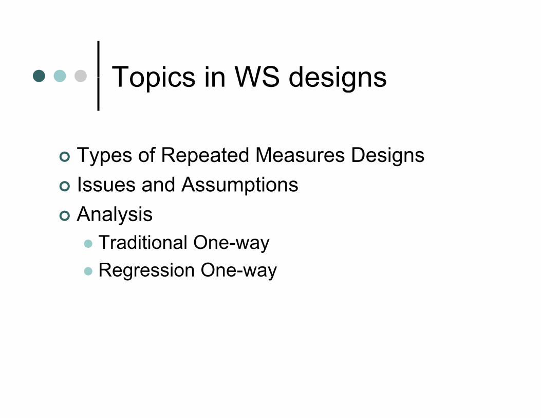
Topics in WS designsTopics in WS designs
Types of Repeated Measures DesignsIssues and AssumptionsIssues and AssumptionsAnalysis
T diti l OTraditional One-wayRegression One-way
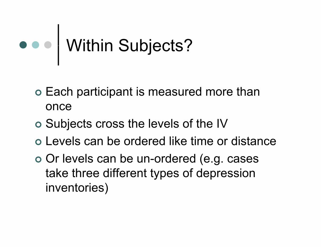
Within Subjects?Within Subjects?
Each participant is measured more than onceonceSubjects cross the levels of the IVLevels can be ordered like time or distanceLevels can be ordered like time or distanceOr levels can be un-ordered (e.g. cases t k th diff t t f d itake three different types of depression inventories)
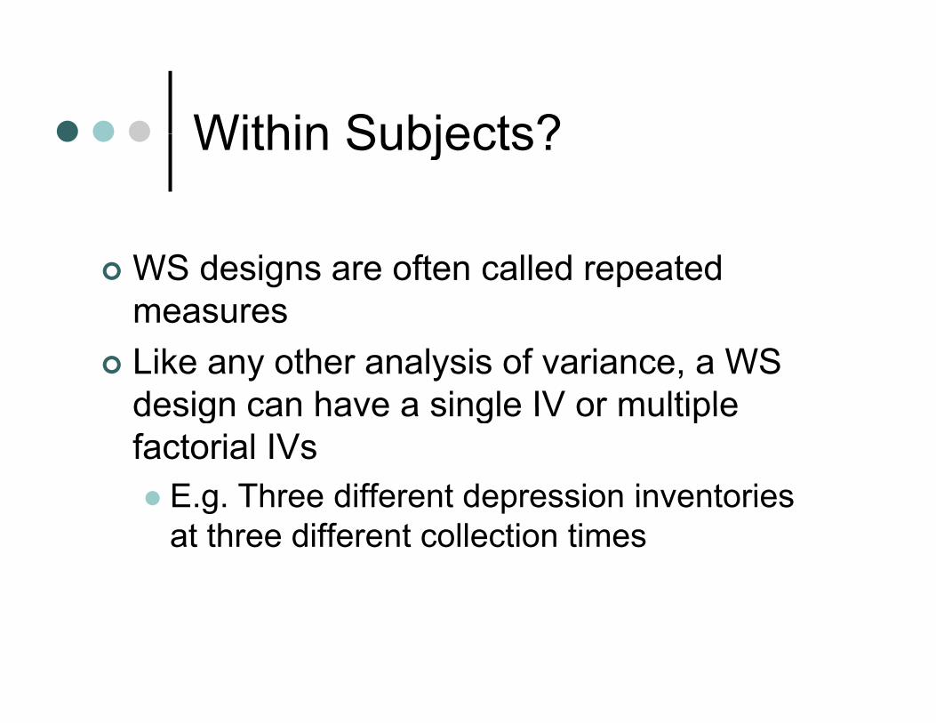
Within Subjects?Within Subjects?
WS designs are often called repeated measuresmeasures Like any other analysis of variance, a WS design can have a single IV or multipledesign can have a single IV or multiple factorial IVs
E g Three different depression inventoriesE.g. Three different depression inventories at three different collection times
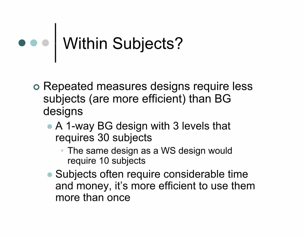
Within Subjects?Within Subjects?
Repeated measures designs require less subjects (are more efficient) than BG j ( )designs
A 1-way BG design with 3 levels that requires 30 subjects
• The same design as a WS design would require 10 subjectsrequire 10 subjects
Subjects often require considerable time and money, it’s more efficient to use them more than once
Within Subjects?Within Subjects?
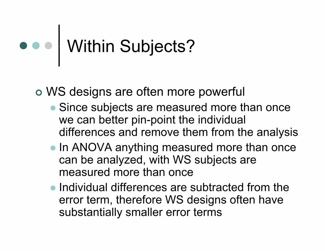
WS designs are often more powerfulSince subjects are measured more than onceSince subjects are measured more than once we can better pin-point the individual differences and remove them from the analysisIn ANOVA anything measured more than once can be analyzed, with WS subjects are measured more than oncemeasured more than onceIndividual differences are subtracted from the error term, therefore WS designs often have , gsubstantially smaller error terms
Types of WS designsTypes of WS designs
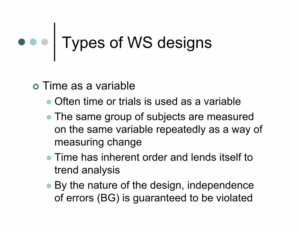
Time as a variableOften time or trials is used as a variableOften time or trials is used as a variableThe same group of subjects are measured on the same variable repeatedly as a way ofon the same variable repeatedly as a way of measuring changeTime has inherent order and lends itself toTime has inherent order and lends itself to trend analysisBy the nature of the design, independenceBy the nature of the design, independence of errors (BG) is guaranteed to be violated
Types of WS designsTypes of WS designs
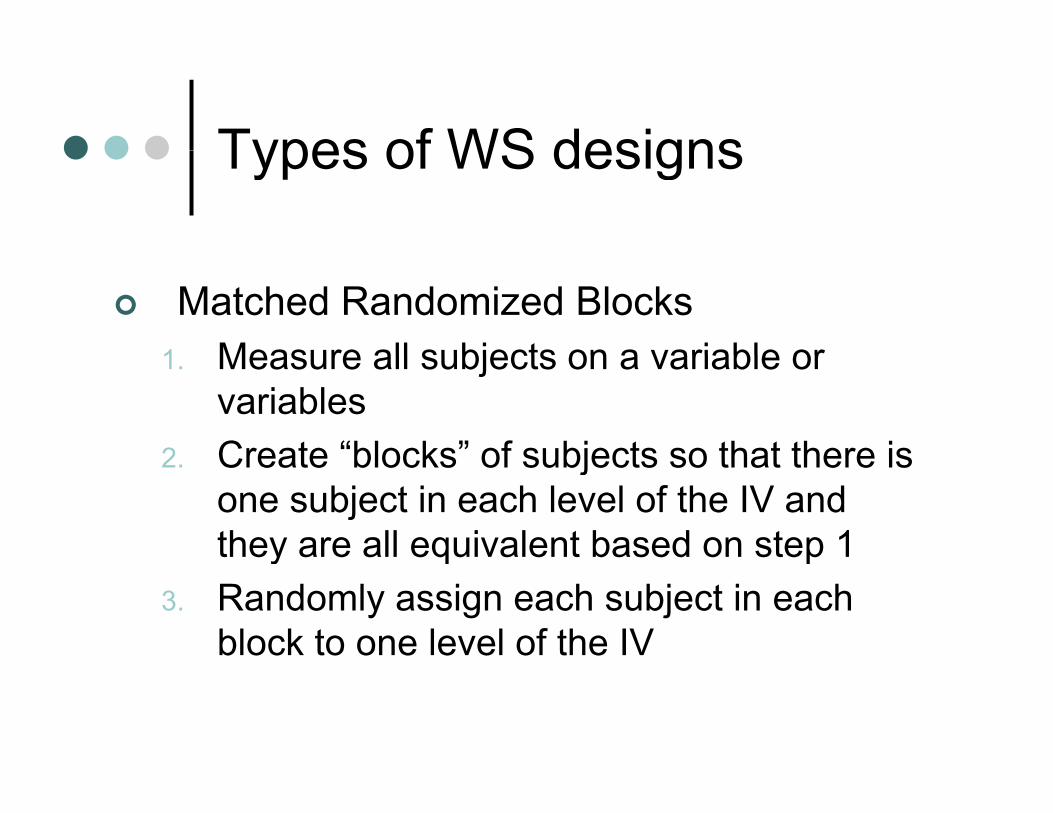
Matched Randomized Blocks1 Measure all subjects on a variable or1. Measure all subjects on a variable or
variables2 Create “blocks” of subjects so that there is2. Create blocks of subjects so that there is
one subject in each level of the IV and they are all equivalent based on step 1y q p
3. Randomly assign each subject in each block to one level of the IV
Issues and AssumptionsIssues and Assumptions
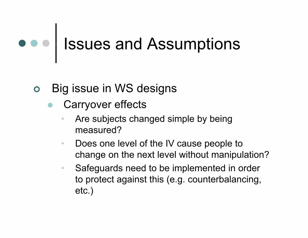
Big issue in WS designsCarryover effectsCarryover effects• Are subjects changed simple by being
measured?• Does one level of the IV cause people to
change on the next level without manipulation?• Safeguards need to be implemented in order
to protect against this (e.g. counterbalancing, etc.))
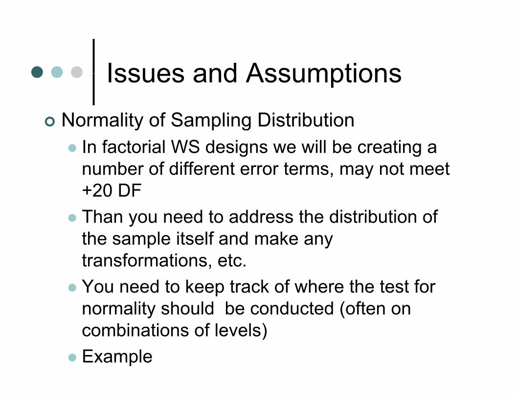
Issues and AssumptionsIssues and AssumptionsNormality of Sampling DistributionNormality of Sampling Distribution
In factorial WS designs we will be creating a number of different error terms, may not meetnumber of different error terms, may not meet +20 DFThan you need to address the distribution of ythe sample itself and make any transformations, etc.You need to keep track of where the test for normality should be conducted (often on
bi ti f l l )combinations of levels)Example
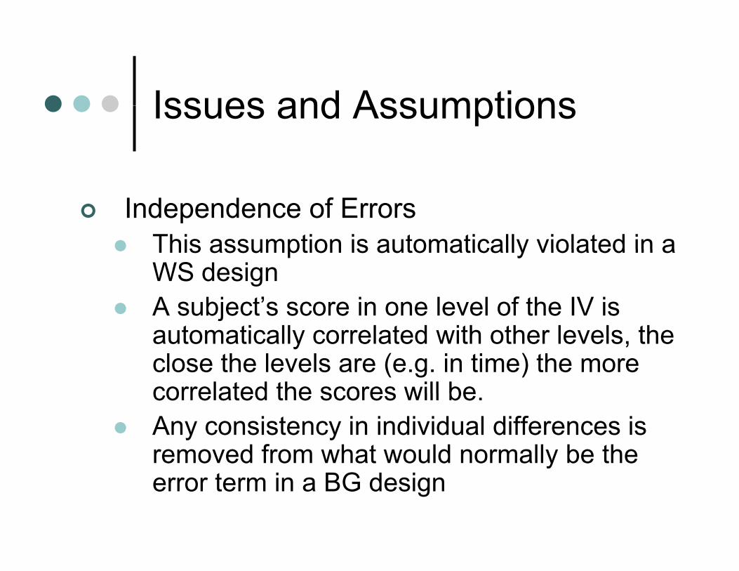
Issues and AssumptionsIssues and Assumptions
Independence of ErrorsThis assumption is automatically violated in aThis assumption is automatically violated in a WS designA subject’s score in one level of the IV is automatically correlated with other levels, the close the levels are (e.g. in time) the more correlated the scores will becorrelated the scores will be.Any consistency in individual differences is removed from what would normally be the yerror term in a BG design
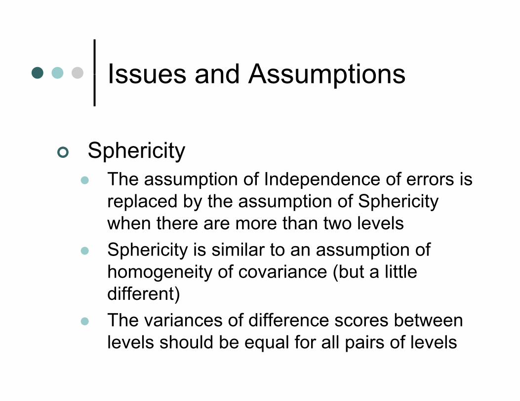
Issues and AssumptionsIssues and Assumptions
SphericityTh ti f I d d f iThe assumption of Independence of errors is replaced by the assumption of Sphericity when there are more than two levelswhen there are more than two levelsSphericity is similar to an assumption of homogeneity of covariance (but a littlehomogeneity of covariance (but a little different)The variances of difference scores between levels should be equal for all pairs of levels
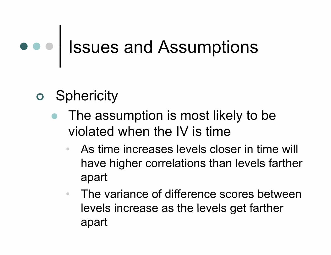
Issues and AssumptionsIssues and Assumptions
SphericityTh ti i t lik l t bThe assumption is most likely to be violated when the IV is time• As time increases levels closer in time will
have higher correlations than levels farther apartapart
• The variance of difference scores between levels increase as the levels get fartherlevels increase as the levels get farther apart
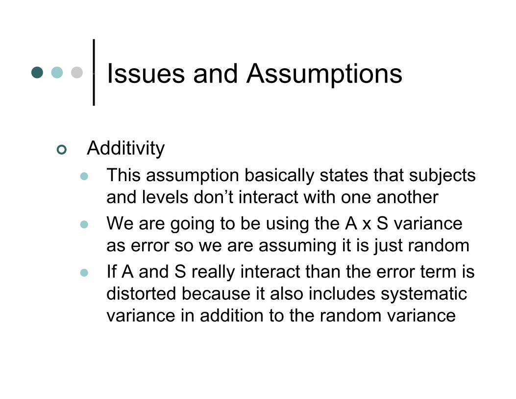
Issues and AssumptionsIssues and Assumptions
AdditivityThis assumption basically states that subjectsThis assumption basically states that subjects and levels don’t interact with one anotherWe are going to be using the A x S varianceWe are going to be using the A x S variance as error so we are assuming it is just randomIf A and S really interact than the error term isIf A and S really interact than the error term is distorted because it also includes systematic variance in addition to the random variance
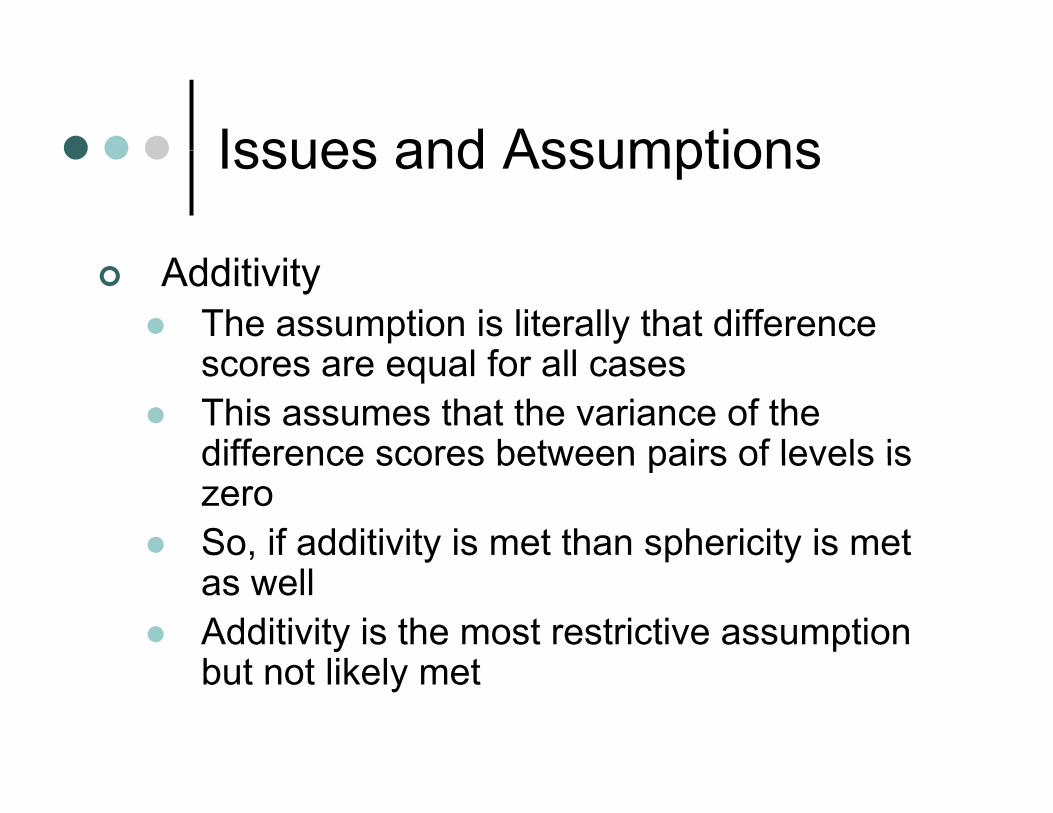
Issues and AssumptionsIssues and Assumptions
AdditivityThe assumption is literally that difference
l f llscores are equal for all casesThis assumes that the variance of the difference scores between pairs of levels isdifference scores between pairs of levels is zeroSo, if additivity is met than sphericity is met y p yas wellAdditivity is the most restrictive assumption b t t lik l tbut not likely met
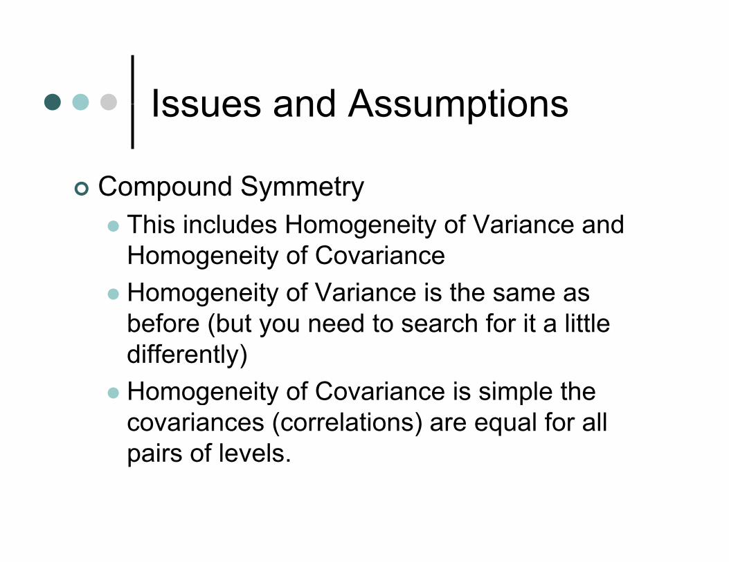
Issues and AssumptionsIssues and Assumptions
Compound SymmetryThis includes Homogeneity of Variance and H i f C iHomogeneity of CovarianceHomogeneity of Variance is the same as b f (b t d t h f it littlbefore (but you need to search for it a little differently)Homogeneity of Covariance is simple theHomogeneity of Covariance is simple the covariances (correlations) are equal for all pairs of levelspairs of levels.
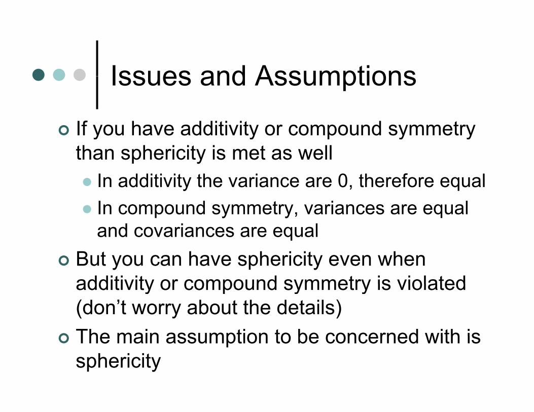
Issues and AssumptionsIssues and Assumptions
If you have additivity or compound symmetryIf you have additivity or compound symmetry than sphericity is met as well
In additivity the variance are 0 therefore equalIn additivity the variance are 0, therefore equalIn compound symmetry, variances are equal and covariances are equaland covariances are equal
But you can have sphericity even when additivity or compound symmetry is violatedadditivity or compound symmetry is violated (don’t worry about the details)The main assumption to be concerned with isThe main assumption to be concerned with is sphericity
Issues and AssumptionsIssues and Assumptions
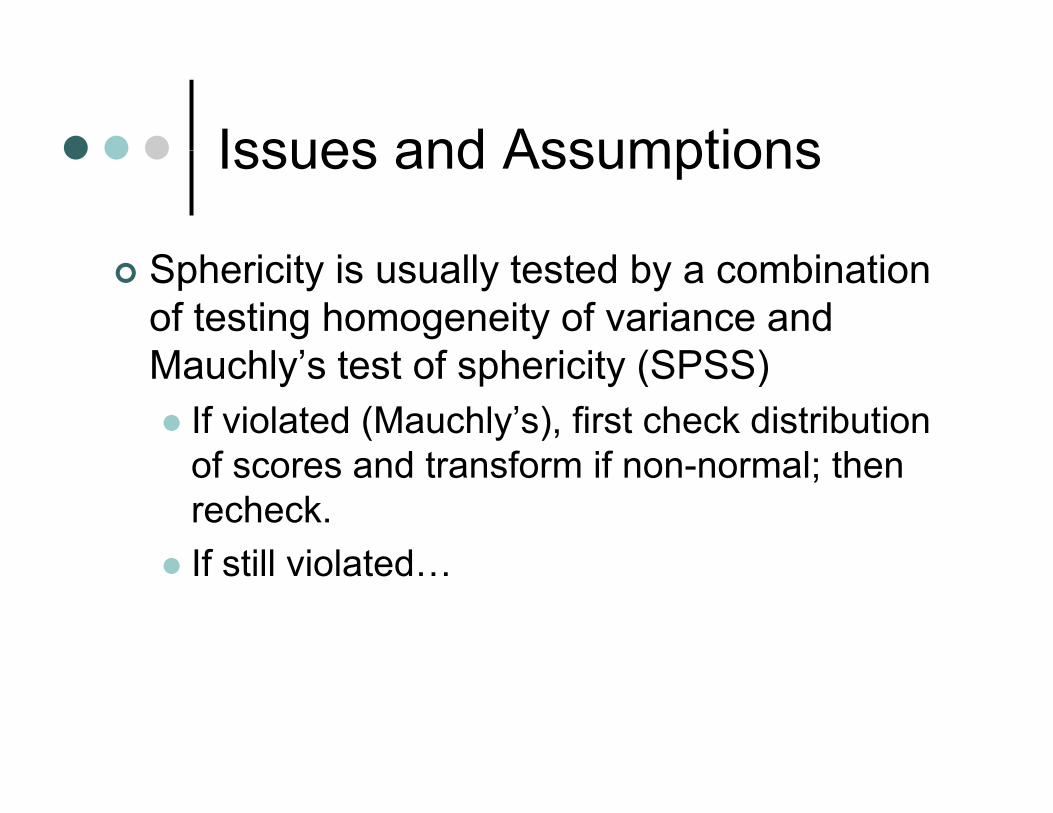
Sphericity is usually tested by a combination of testing homogeneity of variance and M hl ’ t t f h i it (SPSS)Mauchly’s test of sphericity (SPSS)
If violated (Mauchly’s), first check distribution of scores and transform if non normal thenof scores and transform if non-normal; then recheck.If still violatedIf still violated…
Issues and AssumptionsIssues and Assumptions
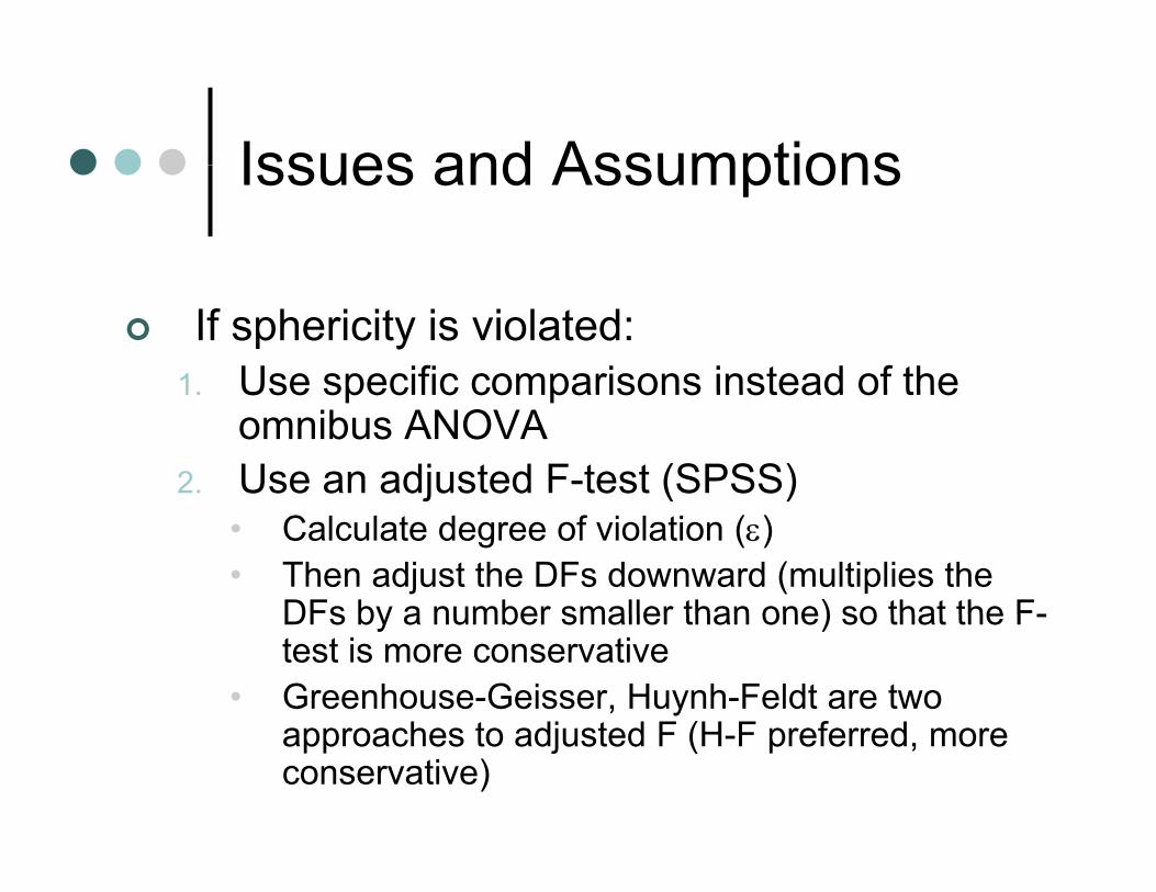
If sphericity is violated:1 Use specific comparisons instead of the1. Use specific comparisons instead of the
omnibus ANOVA2. Use an adjusted F-test (SPSS)
• Calculate degree of violation (ε)• Then adjust the DFs downward (multiplies the
DFs by a number smaller than one) so that the F-DFs by a number smaller than one) so that the F-test is more conservative
• Greenhouse-Geisser, Huynh-Feldt are two h t dj t d F (H F f dapproaches to adjusted F (H-F preferred, more
conservative)
Issues and AssumptionsIssues and Assumptions
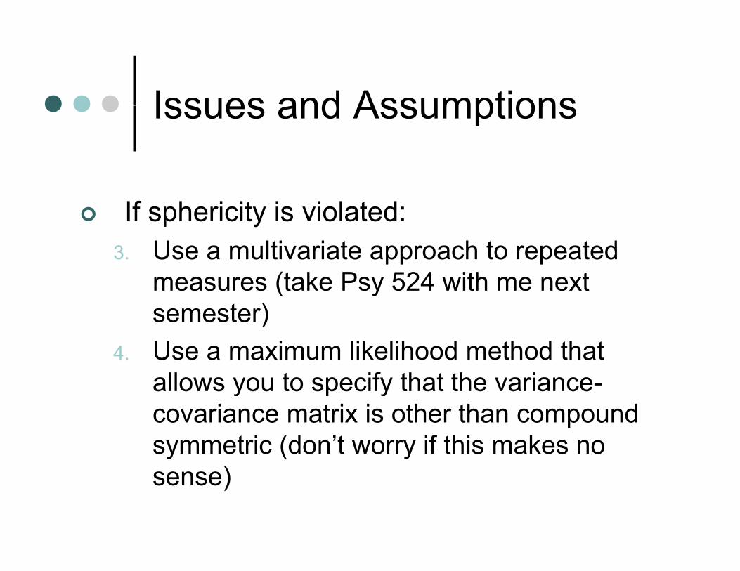
If sphericity is violated:3 Use a multivariate approach to repeated3. Use a multivariate approach to repeated
measures (take Psy 524 with me next semester)semester)
4. Use a maximum likelihood method that allows you to specify that the variance-y p ycovariance matrix is other than compound symmetric (don’t worry if this makes no sense)
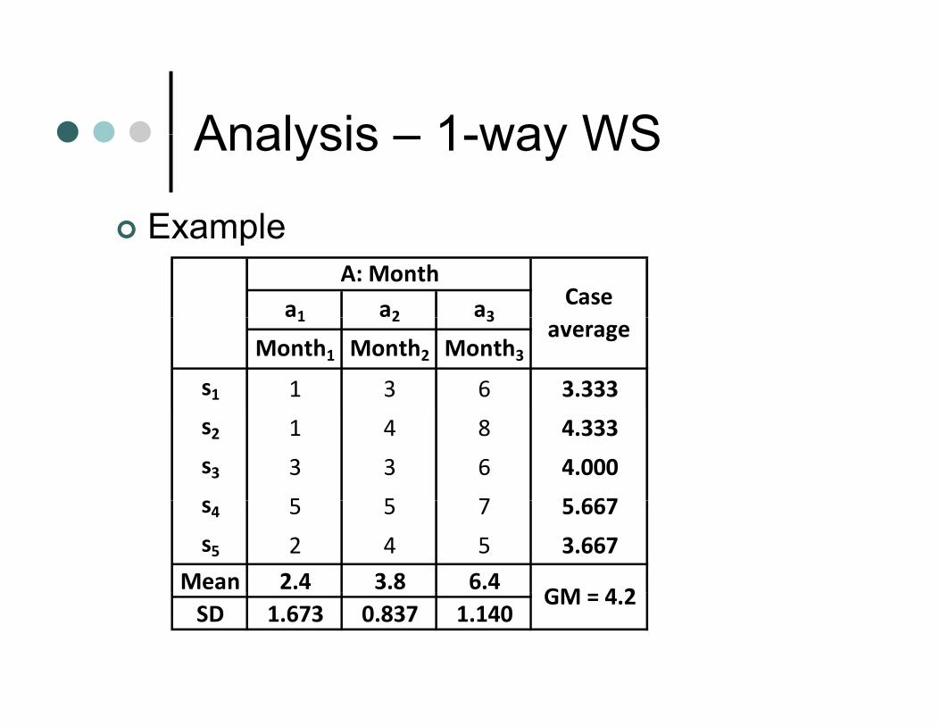
Analysis 1 way WSAnalysis – 1-way WS
ExampleExample
a1 a2 a3
A: MonthCase
1 2 3
Month1 Month2 Month3s1 1 3 6 3.333
average
s2 1 4 8 4.333
s3 3 3 6 4.000
s 5 5 7 5 667s4 5 5 7 5.667
s5 2 4 5 3.667
Mean 2.4 3.8 6.4GM 4 2
SD 1.673 0.837 1.140GM = 4.2
Analysis 1 way WSAnalysis – 1-way WS
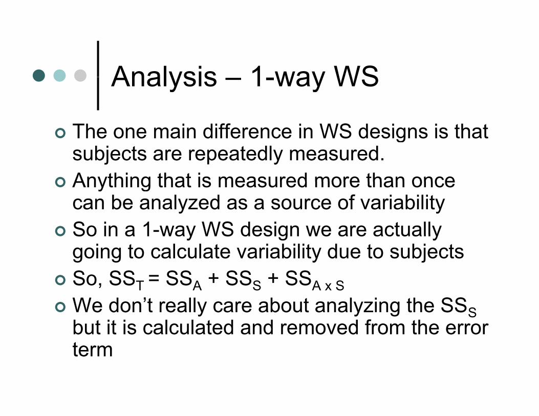
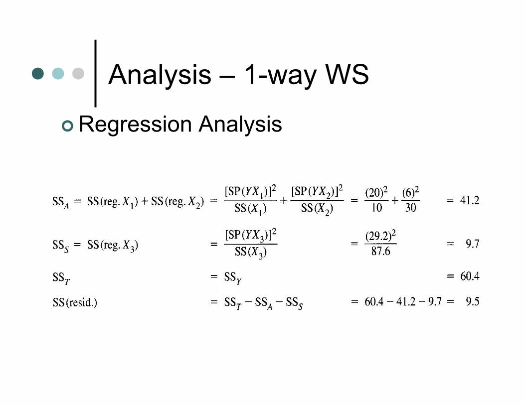
The one main difference in WS designs is thatThe one main difference in WS designs is that subjects are repeatedly measured. Anything that is measured more than onceAnything that is measured more than once can be analyzed as a source of variabilitySo in a 1-way WS design we are actuallySo in a 1 way WS design we are actually going to calculate variability due to subjectsSo, SST = SSA + SSS + SSA x S, T A S A x SWe don’t really care about analyzing the SSSbut it is calculated and removed from the error term
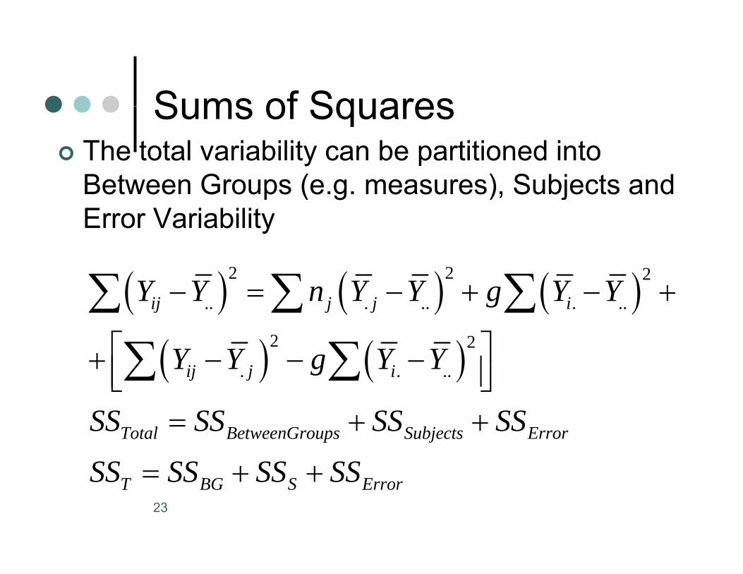
Sums of SquaresSums of SquaresThe total variability can be partitioned into B t G ( ) S bj t dBetween Groups (e.g. measures), Subjects and Error Variability
( ) ( ) ( )2 2 2.. . .. . ..ij j j iY Y n Y Y g Y Y− = − + − +∑ ∑ ∑
( ) ( )2 2. . ..ij j iY Y g Y Y⎡ ⎤+ − − −⎢ ⎥⎣ ⎦∑ ∑
Total BetweenGroups Subjects ErrorSS SS SS SS
SS SS SS SS
= + +
+ +23
T BG S ErrorSS SS SS SS= + +
Analysis 1 way WSAnalysis – 1-way WS
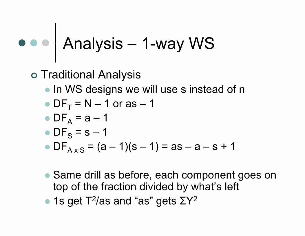
Traditional AnalysisTraditional AnalysisIn WS designs we will use s instead of nDF = N 1 or as 1DFT = N – 1 or as – 1DFA = a – 1 DF = s – 1DFS = s – 1DFA x S = (a – 1)(s – 1) = as – a – s + 1
Same drill as before, each component goes on top of the fraction divided by what’s left1s get T2/as and “as” gets ΣY2
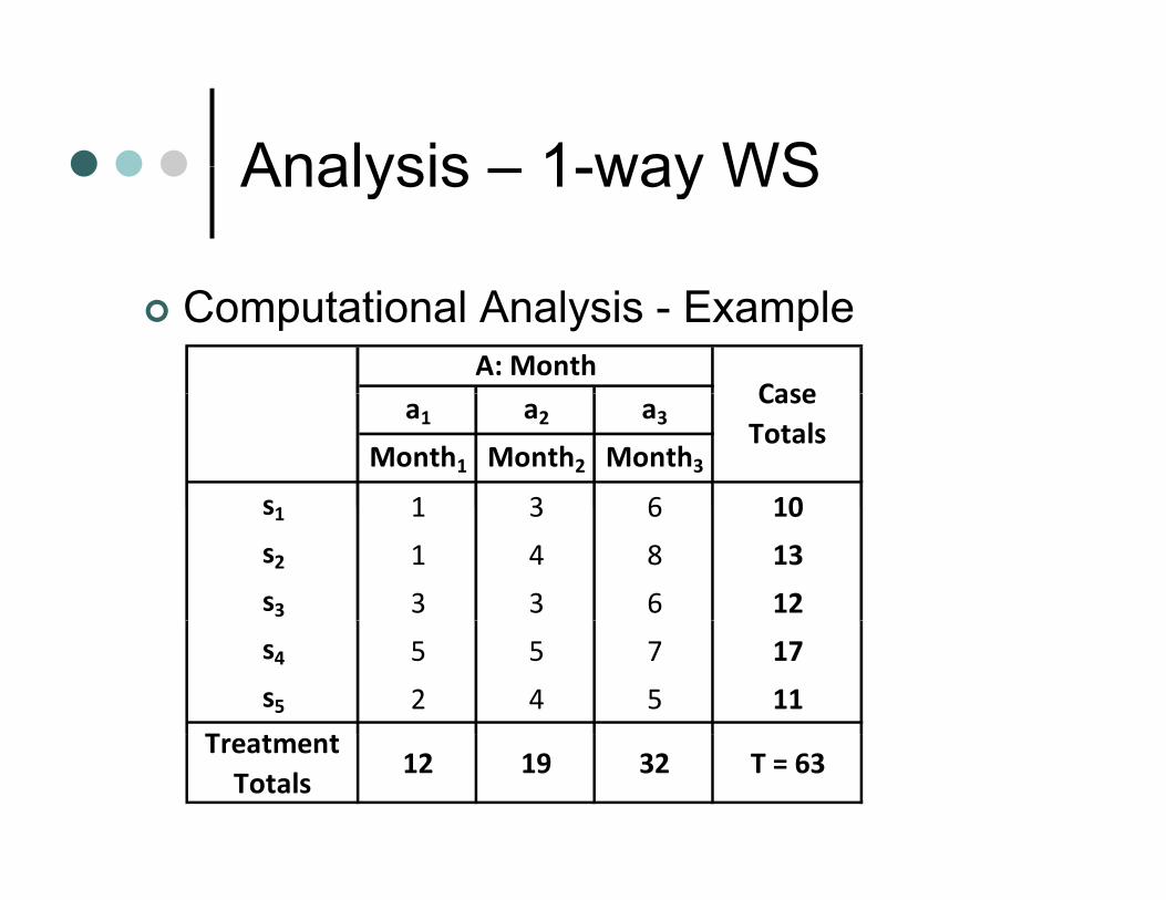
Analysis 1 way WSAnalysis – 1-way WS
Computational Analysis - ExampleA: Month
Casea1 a2 a3Month1 Month2 Month3
s 1 3 6 10
Case Totals
s1 1 3 6 10
s2 1 4 8 13
s3 3 3 6 12
s4 5 5 7 17
s5 2 4 5 11
TTreatment Totals
12 19 32 T = 63
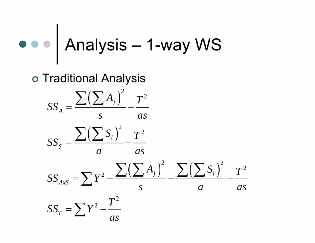
Analysis 1 way WSAnalysis – 1-way WS
T diti l A l iTraditional Analysis
( )22
jA TSS =∑ ∑
( )22
A
i
SSs as
S T
= −
∑ ∑( )
( ) ( )2 22
iS
TSSa as
A S
= −∑ ∑
∑ ∑ ∑ ∑( ) ( ) 22
2
j iAxS
A S TSS Ys a as
= − − +∑ ∑ ∑ ∑∑2
2T
TSS Yas
= −∑
Analysis 1 way WSAnalysis – 1-way WS
Traditional Analysis - Example
2 2 2 212 19 32 63 1529 3 9692 2 2 2
2 2 2 2 2
12 19 32 63 1,529 3,969 305.8 264.6 41.25 3(5) 5 15
10 13 12 17 11 823
ASS + += − = − = − =
2 2 2 2 210 13 12 17 11 823264.6 264.6 274.3 264.6 9.73 3
325 305 8 2743 2646 9 5
SSS
SS
+ + + += − = − = − =
+325 305.8 274.3 264.6 9.5325 264.6 60.4
AxS
T
SSSS
= − − + == − =
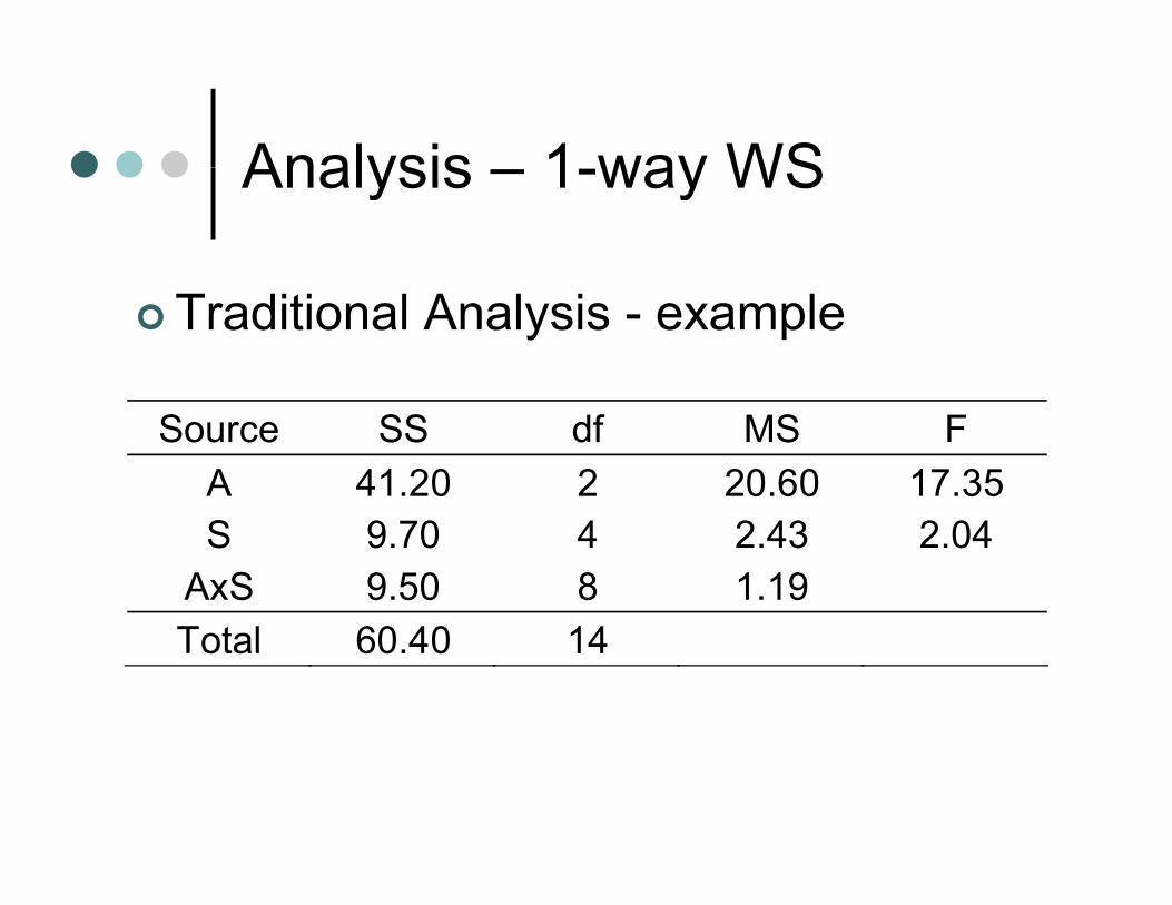
Analysis 1 way WSAnalysis – 1-way WS
Traditional Analysis - example
Source SS df MS F A 41.20 2 20.60 17.35 S 9.70 4 2.43 2.04
AxS 9.50 8 1.19 Total 60.40 14
Analysis 1 way WSAnalysis – 1-way WS
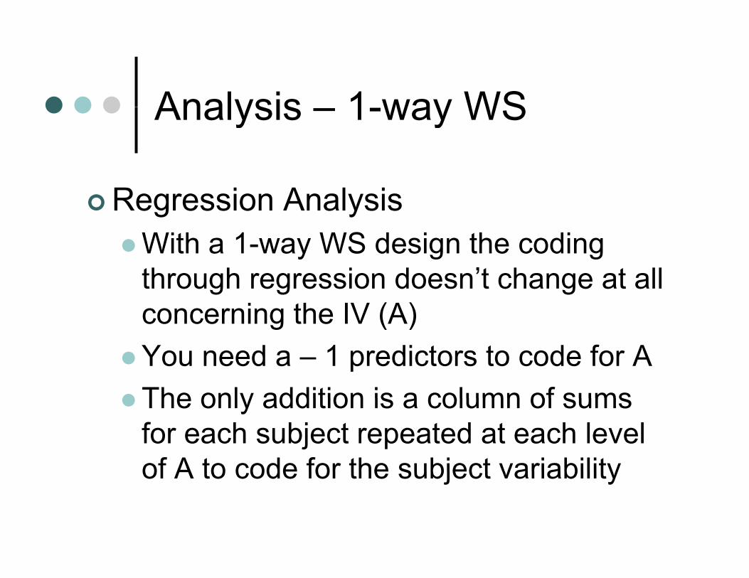
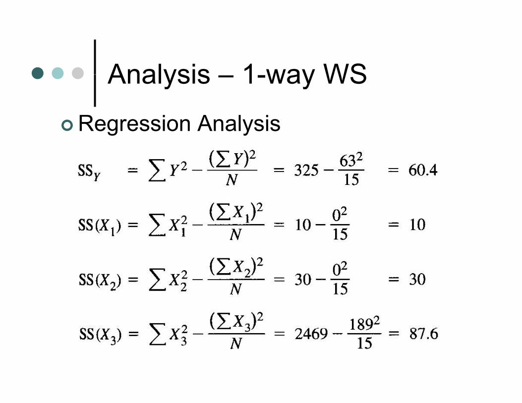
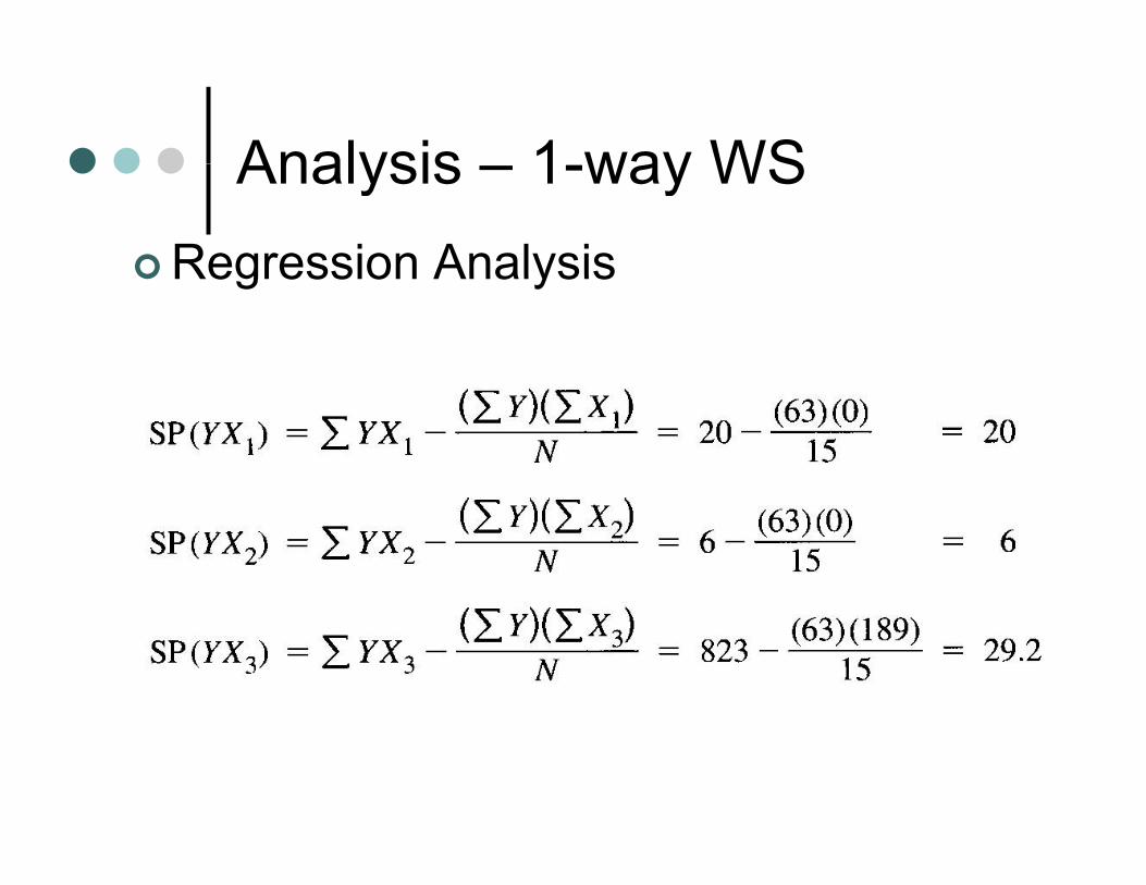
Regression AnalysisWith a 1-way WS design the codingWith a 1 way WS design the coding through regression doesn’t change at all concerning the IV (A)g ( )You need a – 1 predictors to code for AThe only addition is a column of sumsThe only addition is a column of sums for each subject repeated at each level of A to code for the subject variabilityof A to code for the subject variability
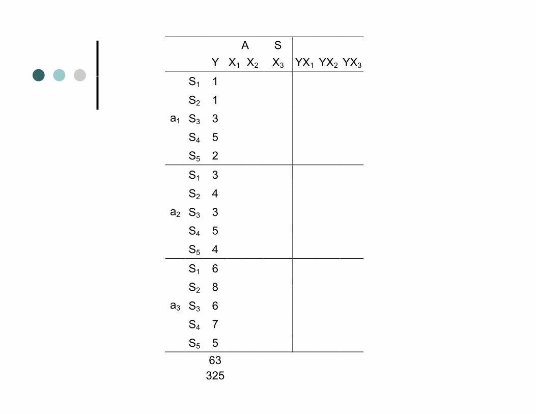
A S Y X1 X2 X3 YX1 YX2 YX3
S1 1
S2 1 S3 3 a1
S4 5 S5 2
S1 3 S2 4
S3 3 S4 5
a2
S4 5 S5 4
S1 6 S 8S2 8
S3 6 S4 7
a3
S5 5 63 325
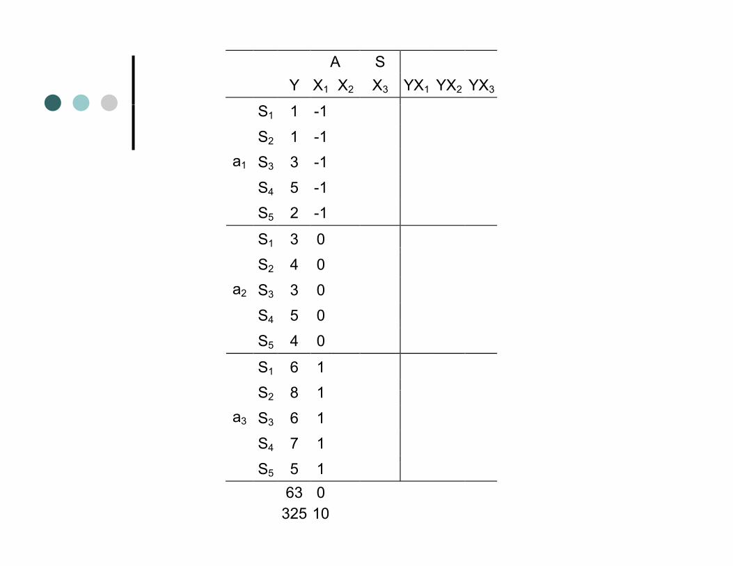
A S Y X1 X2 X3 YX1 YX2 YX3
S1 1 -1
S2 1 -1 S3 3 -1 a1
S4 5 -1 S5 2 -1
S1 3 0 S2 4 0
S3 3 0 S4 5 0
a2
S4 5 0 S5 4 0
S1 6 1 S 8 1S2 8 1
S3 6 1 S4 7 1
a3
S5 5 1 63 0 325 10
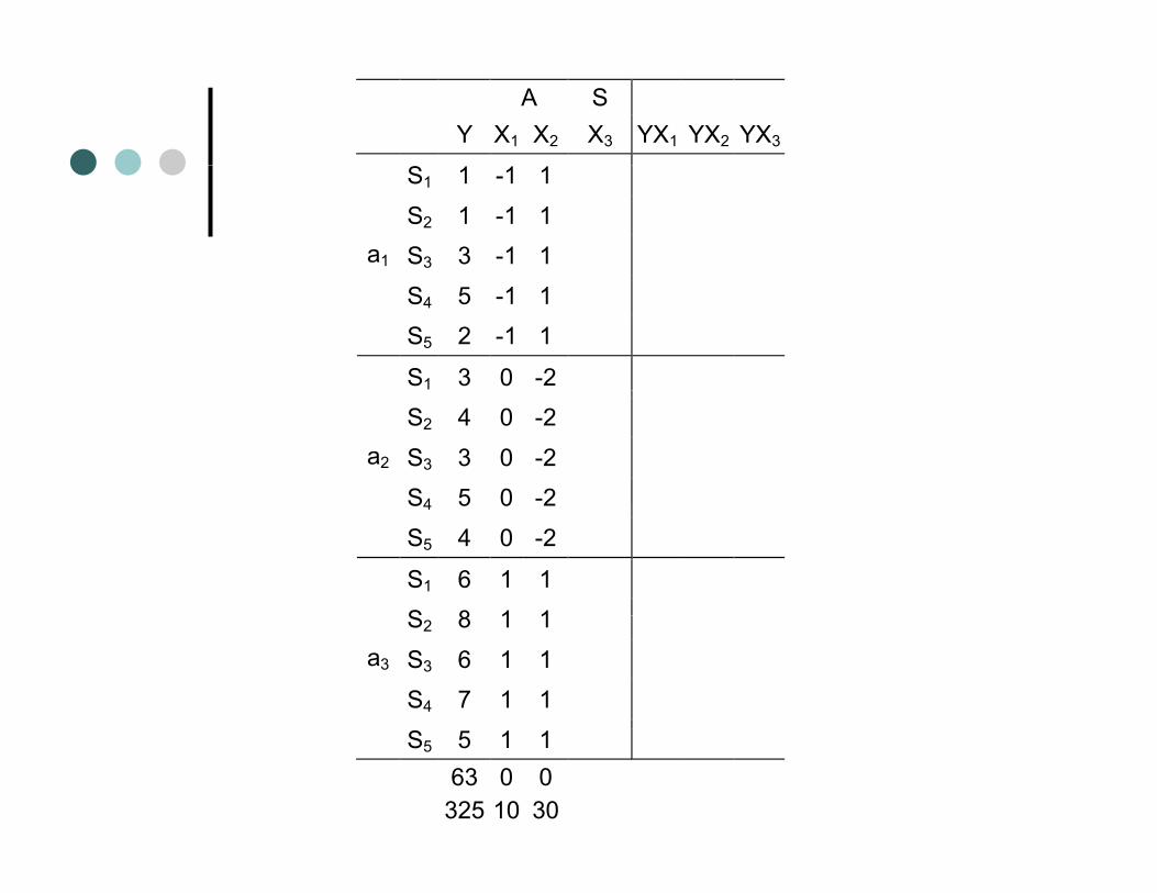
A S Y X1 X2 X3 YX1 YX2 YX3
S1 1 -1 1
S2 1 -1 1 S3 3 -1 1 a1
S4 5 -1 1 S5 2 -1 1
S1 3 0 -2 S2 4 0 -2
S3 3 0 -2 S4 5 0 -2
a2
S4 5 0 2 S5 4 0 -2
S1 6 1 1 S 8 1 1S2 8 1 1
S3 6 1 1 S4 7 1 1
a3
S5 5 1 1 63 0 0 325 10 30
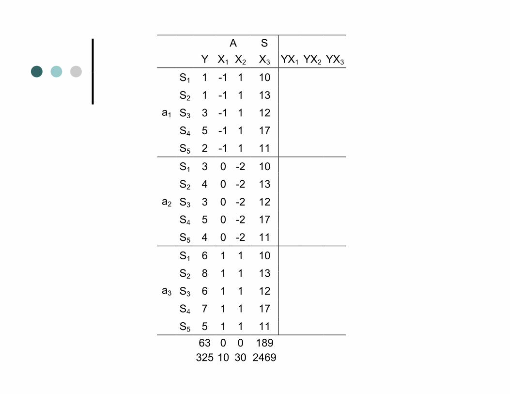
A S Y X1 X2 X3 YX1 YX2 YX3
S1 1 -1 1 10
S2 1 -1 1 13 S3 3 -1 1 12 a1
S4 5 -1 1 17 S5 2 -1 1 11
S1 3 0 -2 10 S2 4 0 -2 13
S3 3 0 -2 12 S4 5 0 -2 17
a2
S4 5 0 2 17 S5 4 0 -2 11
S1 6 1 1 10 S 8 1 1 13S2 8 1 1 13
S3 6 1 1 12 S4 7 1 1 17
a3
S5 5 1 1 11 63 0 0 189 325 10 30 2469
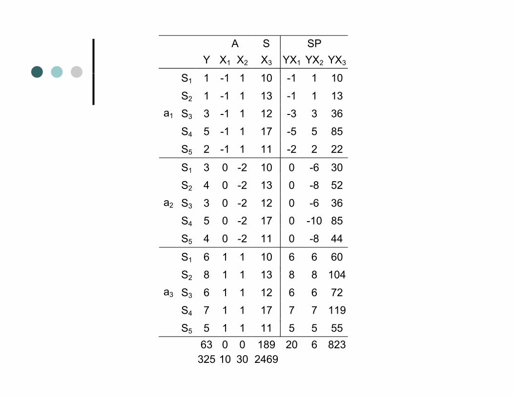
A S SP Y X1 X2 X3 YX1 YX2 YX3
S1 1 -1 1 10 -1 1 10S2 1 -1 1 13 -1 1 13S3 3 -1 1 12 -3 3 36a1
S4 5 -1 1 17 -5 5 85S5 2 -1 1 11 -2 2 22
S1 3 0 -2 10 0 -6 30S2 4 0 -2 13 0 -8 52S3 3 0 -2 12 0 -6 36S4 5 0 -2 17 0 -10 85
a2
S4 5 0 2 17 0 10 85
S5 4 0 -2 11 0 -8 44
S1 6 1 1 10 6 6 60S 8 1 1 13 8 8 104S2 8 1 1 13 8 8 104S3 6 1 1 12 6 6 72S4 7 1 1 17 7 7 119
a3
S5 5 1 1 11 5 5 55 63 0 0 189 20 6 823 325 10 30 2469
Analysis 1 way WSAnalysis – 1-way WS
Regression AnalysisRegression Analysis
Analysis 1 way WSAnalysis – 1-way WSRegression AnalysisRegression Analysis
Analysis 1 way WSAnalysis – 1-way WS
Regression AnalysisRegression Analysis
Analysis 1 way WSAnalysis – 1-way WS
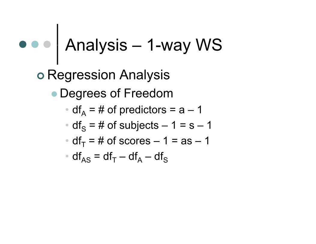
Regression AnalysisRegression AnalysisDegrees of Freedom
df # f di t 1• dfA = # of predictors = a – 1• dfS = # of subjects – 1 = s – 1
df # f 1 1• dfT = # of scores – 1 = as – 1 • dfAS = dfT – dfA – dfS