TESTS OF ENERGY CONSERVATION:AN ECONOMIC APPRAISAL·

by

John F. ScogginsResearch Fellow

Public Utility Research CenterUniversity of Florida

September 12, 1991

*This study provides an overview of methodologies used to evaluate energy conservation programs. It wasprepared in support of a project on Energy Efficiency Incentives for the Florida State Energy Office. SanfordBerg provided helpful comments·on earlier drafts.

-1-

Energy conservation is a goal pursued by most public service commissions across the country.

Since consumers and utility companies may be affected differently by a conservation program, most

public service commissions use several different tests by which to measure the likely effect of

proposed programs.1 This report analyzes the four different tests used by the Florida Public Service

Commission: total resource cost test, participants test, rate impact test and utility cost test.

From an economist's point of view, the rationale for each test is ad hoc. The benefits of a

proposed program may be greater than the costs, according to one test, but not according to the

other three. Since the different tests often give conflicting results, it would be helpful to assess the

four tests using a single theoretic paradigm. A likely candidate for such a paradigm is something

economists call "economic welfare," a long established concept that relies on theories of optimal

economic behavior.

This report is· organized into three main sections. The first section explains the concept of

economic welfare and its relevance in the assessment of energy conservation programs. The second

section analyzes each of the four tests used by the Florida Public Service Commission. The final

section analyzes the "snap-back effect" controversy in the assessment ofenergy conservation programs.

1. Economic Welfare

1.1 The Competitive Standard

Approximations of economic welfare can be obtained·by using empirical estimates of demand

curves and of opportunity costs.2 The basic teclmique is to use a consumer's demand for a quantity

of a good, which is dependent on the good's price, to reveal how much the consumer values different

quantities of that good. Analogously, the quantity of a good that a producer is willing to produce for

1 Tests used by diffelent regulatmycommissions across tile country are very similar. See Burkhart (1990), Costello and Galen (1985),Einhorn (1985), HOObs aad Nelson (1989), and Norland aad Wolf (1985).

2 see Just, Hueth and.Schmitz (1982) for a more complete explanation of economic welfare.

-2-

sale is also dependent on the good's price and reveals the cost of producing different quantities of

the good. Demand and supply curves convey this information because the assumptions concerning

perfectly competitive markets hold. In such markets, the producers strive to maximize their profits

and therefore have incentives to minimize their costs. Consumers want to maximize their utility and

will refuse to pay more for a good than it is worth to them.

The total value of the quantity of a good bought and sold (as determined by the demand

curve) minus the total cost of producing the good (as determined by the supply curve) equals the net

benefit to the population of producing the good. This net benefit to the population is referred to

as economic welfare.

Events that affect the price of a good (price controls), its quantity sold (rationing), or both,

will change "economic welfare. Consequently the advisability of a government action is a function of

its effect on economic welfare. An action that expands the net benefits (gross benefits minus costs)

associated with a commodity increases..economic welfare.

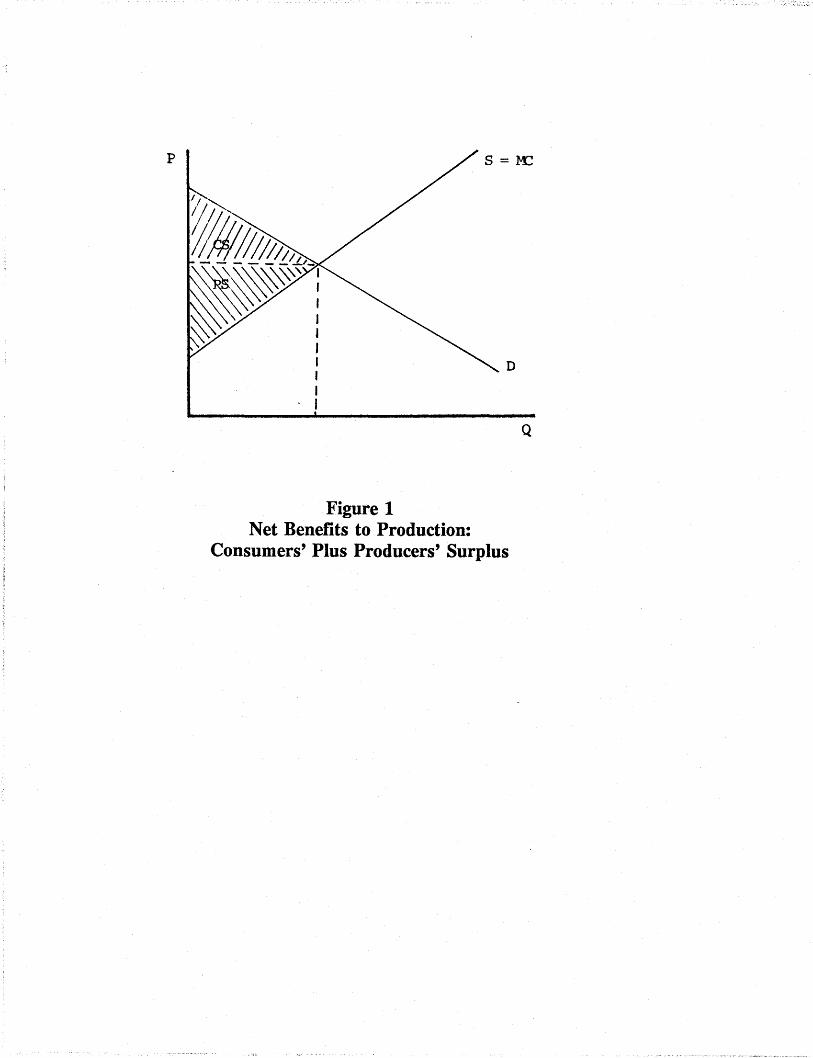
Note that the economic welfare derived from .the·production and consumption of a good can

be broken into two parts: consumer's surplus and prod,ucer's surplus. Consumer's surplus is the

portion of economic welfare enjoyed by consumers while producer's surplus is the portion retained

by the producer. Consumer's surplus is represented by the area below the demand curve

(representing willingness to pay) and above the price charged. Producer's surplus is the area above

the supply curve and below the price charge. Figure 1 shows graphically consumer's surplus and

producer's surplus.

1.2. Market Failure

The equilibrium quantity, as determined by the intersection of the demand and supply curves,

is the quantity that maximizes economic welfare in a perfectly competitive market. Market failure

is the situation where one of the assumptions of perfect competition does not hold for that market.

p

D

Figure 1Net Benefits to Production:

Consumers' Plus Producers' Surplus

Q

-3-

In that case, the equilibrium quantity will not necessarily maximize economic welfare. Costless

government intervention would enhance welfare. The three sources of market failure relevant to

tests of energy conservation programs are (1) the under-investment in efficient energy-using durables

on the part of consumers; (2) external costs of the use of energy; and (3) pricing below the

opportunity cost of electricity.

1.2.1 Under-Investment

Under perfect competition, consumers possess all relevant information and choose their

purchases rationally, that is, without obvious error. However, in the purchase of energy-using

durables, there. is evidence that consumers violate this condition of rationality.3 By purchasing more

expensive but more efficient energy-using durables, many consumers could either enjoy more of the

end-use gOOd that the energy-using durable produces (such as cooled air) without an increase in total

cost of production or consume the same amount of the end-use good at a lower total cost.

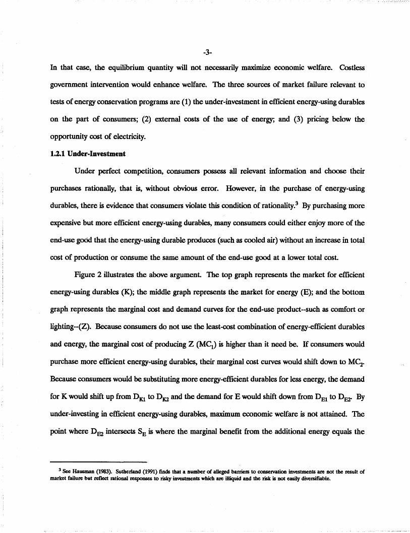
Figure 2 illustrates the above argument. The top graph represents the market for efficient

energy-using durables (K); the middle •graph represents the market for energy (E); and the bottom

graph represents the marginal cost and demand curves for the end-use product--such as comfort or

lighting--(Z). Because consumers do not use the least-eost combination of energy-efficient durables

and energy, the marginal cost of producing Z (MCl ) is higher than it need be. If consumers would

purchase more efficient energy-using durables, their marginal cost curves would shift down to MC2•

Because consumers would be substituting more energy-efficient durables for less energy, the demand

for K would shift up from DKl to DK2 and the demand for E would shift down from DEI to Dm. By

under-investing in efficient energy-using durab1es,maximum economic welfare is not attained. The

point where Dm intersects SE is where the marginal benefit from the additional energy equals the

3 See Hausman (1983). Sutherland (1991) fInds that a number of alleged barriers to coaservation investments are not the result ofmarket failure ·but reflect rational :responses to risky investments which are illiquid and the risk is not easily diversifiable.

$

$

$

k (Energy-Using Durable)

E (Energy)

Z (End-Use Good)

Figure 2Net Benefits of Increased .Investment in

Efficient Energy-Using Durables ·(With Small Snap-Back Effect)

-4-

opportunity cost. Therefore~ is the quantity that maximizes the sum of consumer's and producer's

surplus. With every extra unit of consumption above ~, producer's surplus increases but consumer's

surplus decreases by a larger amount. H E1 is the quantity consumed, the loss of the sum of

consumer's surplus and producer's surplus is represented by the shaded area in the middle graph.

The increase in end-use consumption from Zl to ~ caused by the decrease in the marginal

cost curve is known as the "snap-back effect." This effect will reduce the possible energy savings of

a program that attempts to improve the energy-efficiency of energy-using durables. Notice that the

slope of the demand curve for the end-use good (Dz) in Figure 2 is depicted as being very steep

(inelastic). In this case, the snap-back effect is relatively small, and the associated decrease in energy

consumption (E1 -~ is relatively large. Conversely, the slope of Dz at the bottom of Figure 3 is

relatively shallow making the snap-back.effect large. The decrease in energy demand in Figure 3 is

therefore relatively small (E1 - ~). Notice that the shaded area in Figure 3, representing the loss

of economic welfare from under-investment in efflCientenergy-using durables, is also relatively small.

In general, the smaller the snap-back effect, the greater is the loss of economic welfare from the

under-investment in efficient energy-using durables.

Although the stated purpose of an energy conservation program may be to decrease the

consumption of energy, economic welfare measures do not weigh a decrease in energy consumption

any more than they weigh an increase in end-use good consumption (the snap-back effect). Because

of this, the use of economic welfare in the testing of energy conservation programs is potentially

controversial. This controversy will be discussed later in greater detail.

1.2.2 Extemal Cost

Another necessary condition for a perfectly competitive market to maximize economic welfare

is that all the costs of producing a good are bome by the producers. Otherwise, the supply curve

does·not represent the social.marginal.cost of producing the good. If the good is ·priced at the private

$

$

$

DK2

K (Energy-Using Durables)

E (Energy)

1 Z (End-Use Good)

Figure 3Net Benefits of Increased Investment in

Efficient Energy-Using Durables(With Large Snap-Back Effect)

-5-

opportunity cost, the price is low relative to the full costs borne by society when additional units of

output are produced.

Pollution is the most frequently cited example of an external cost, and the burning of fossil

fuels is a significant source of pollution. Of course, the extent to which the new Acid Rain

legislation, the Clean Air Act, and other laws require relatively pollution-free production processes,

production costs rise and the externalities are reduced. Another kind of external cost could be a

reliance on foreign suppliers of fossil fuels, which could affect national security (and defense

expenditure).

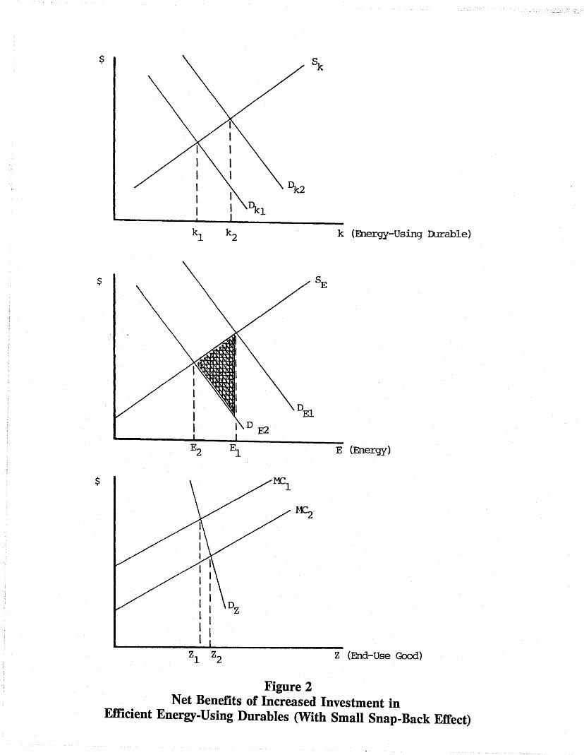
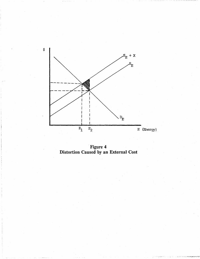
Figure 4 is used to illustrate externalities. The marginal cost to society of producing energy

is represented by the supply curve SE + X. The economic welfare-maximizing quantity is E t.

However, since only some of the costs of producing the good are borne by the producers, too low

a price is charged, and too high a quantity is consumed (~). By taxing the good, the consumption

of energy could be reduced from ~ to E t , and economic welfare could be increased by the amount

equal to the shaded area, as the external cost is reduced to where· the marginal valuation placed on

additional output is just equal to the marginal social cost associated with that unit of output

The above paragraph is a standard analysis of an external cost's effect on economic welfare.

However, in the case of regulated utilities, the situation is a little more involved. It is possible that

the external costs of production associated with old productive capacity would be much higher than

the external costs associated with new productive capacity. The technology of the new productive

capacity might bum fossil fuels more cleanly.

Unfortunately, the exact welfare gain from decreasing energy consumption is difficult to

ascertain because the exact external cost of energy production is hard to measure. But the external

cost reduction from an energy conservation program should be roughly proportional to the reduction

$

E (Energy)

Figure 4Distortion Caused by an External Cost

-6-

in energy consumption: many tests of conservation programs rely solely on reductions in energy

production (regardless of the age of the electricity generating unit or actual emission reductions).

1.2.3 Pricing Below Opportunity Costs

The typical utility company is a regulated monopoly.4 In the multi-firm competitive case the

demand and supply (marginal cost) curves intersect such that the marginal firm earns normal profits.

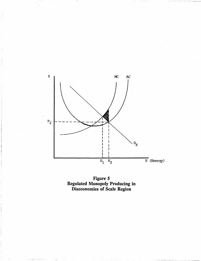
This condition does not hold for a monopoly however. It will sometimes be the case that the demand

for energy will intersect the average cost curve in the diseconomies of scale region (i.e. the quantities

of E where average cost in increasing). This case is illustrated in Figure 5.

In order for the utility to only recoup the cost of producing energy, if it is constrained to a

charge uniform price for each unit of output, then price will equal the average cost of production (at

~). However, economic welfare is maximized when the price is equal to the marginal cost (at E1).

Theaverage-cost price is too low at that quantity of production, and the resulting quantity demanded

is too high. The loss of economic welfare is represented by the shaded area in Figure 5.

The reasoning behind this result is that the cost of adding productive capacity is very high

relative to the average cost. A conservation program that reduced the demand for energy would

increase economic welfare because the avoided capacity and operating costs would be greater than

the benefits sacrificed from reduced energy consumption.

Alternatively, ifhistorical capacity costs are low relative to incremental capacity costs, average

cost pricing leads to similar "underpricing" of electricity relative to social opportunity costs. Public

Service Commissions could provide the correct (higher) price signal to consumers without ·unduly

burdening them if an inverted rate design is adopted. Marginal price would then be greater than the

average price, and uneconomic consumption would be discouraged.

4 See Berg and Tschirhart (1988).

$ AC

Figure 5Regulated Monopoly Producing in

Diseconomies of Scale Region

E (Energy)

-7-

To summarize, under-investment in efficient energy-using durables leads to a marginal

operating cost curve (for households) that is too high and end-use good consumption that is too low.

External costs of energy consumption lead to a marginal cost curve (for utilities) which is too low and

end-use consumption that is too high. Operating in the diseconomies of scale region of the long run

average cost curve, monopoly regulated to price at average cost charges a price that is too low to

maximize economic welfare. All three sources of market failure lead to excessive energy

consumption. By increasing the efficiency ofenergy-using durables, the demand for energy is reduced

(although this is partially offset by a reduction in the marginal cost curve· for producing comfort,

lighting, or other end-use goods). In addition, by internalizing the external costs of energy

consumption, more resources would be devoted to end-use good production, and less energy would

be consumed. Lastly, a pricing system that equates the price with the marginal cost of production

would decrease energy consumption when the regulated monopoly experienced long run diseconomies

of scale.

1.3. Distributional (or Equity) Concerns

When. a government action increases overall economic welfare, the economic welfare of a

particular party is often diminished. An example would be a conservation program that succeeds in

increasing energy-.efficiency and lowering energy demand. As noted in the explanation of the middle

graph in Figure 2, the sum of consumer's surplus and producer's surplus would increase, but

producer's surplus would decrease. This potential drop in producer's surplus isa disincentive for

utilities to implement conservation programs and is the main reason why so many different tests are

used to assess energy conservation programs.S

The strict use of consumer's and producer's surplus as a measure of economic welfare implies

that a transfer of a dollar from one individual to another would leave economic welfare unchanged.

S See Cicchetti (1989).

-8-

Because such conclusions require that all individuals have identical preferences, abilities and wealth,

economists shy away from making such interPersonal comparisons.

Nevertheless, economists can justify the use of the sum of consumer's and producer's surplus

because of a concept called "Pareto efficiency." Simply put, the distributional problem most

government actions create can be remedied through a kind of compensation system. An example

would be where, instead of allowing consumers to retain all the benefits of a conservation program,

the conservation program would be designed to allow the utility to share in the benefits. The net

effect on consumer's and producer's surplus would be the same under either policy, but the latter

would alleviate the distnbutional problem.

2. Tests of Energy Conservation Programs6

2.1. Rate· Impact Test

The. benefits in this test are defiBedas the avoided supply costs as well as any increased

revenues. The costs include program costs incurred by the utility, the incentives paid to participants

and any increased supply costs. The costs also include any decrease in revenues.

The net benefit of a conservation program as defined by the rate imPact test is the same as

the change in producer's surplus. As illustrated in Figure 6a, a program that increased investment

in efficient energy-using durables would decrease energy consumption from E1 to ~and decrease

the pricefrom P1 to P2• The utility's revenue falls by the shaded areas A and B. But the utility's cost

falls by the shaded area B. Therefore the utility's decrease in profits is represented by the shaded

area A

2.2. Utility Cost Test

The benefits and costs for this test are the same as for the rate impact test except that

changes in revenue are excluded. The net benefit of a conservation program as defined by this test

6 See Florida Public Service Commission· (1990).

$

Figure 6a

$

L J3~_------zZ (End-Use Qxx1)Zl Z2

Figure 6b

Figure 6cDK2

· Durable)L_-~~~------KK(Energy-Uslng

$

rvation InvestmentImpacts of a Conse

-9-

is represented by the shaded area B in Figure 6a. This is equal to the decrease in producer's surplus

(area A) minus the decrease in revenue (area A + B). The above illustration indicates that a

program that lowers revenue may have positive net benefits according to the utility cost test but

negative net benefits according to the rate impact test.

2.3. Participants Test

The benefits for this test include reductions in the consumers' bills, incentives paid by the

utility or other third party and any tax credits received. The costs include increases in the participant

customers' bills (to pay for the incentives), equipment and materials purchased, ongoing operation

and maintenance costs and any equipment removal costs.

According to the definitions, the net benefits for this test equal the change in consumer's

surplus excluding the snap-back effect. Figures 6b and 6c illustrate this quantity. The net benefit

to consumers of a program that induced· them to purchase more efficient energy-using durables would

equal the increase in consumers's surplus (area E + F in Figure 6b) minus the increase in

expenditures on energy-using durables (area H + I in Figure 6c). The gross benefit of the snap-back

effect (ignoring costs) is the value ofthe increased consumption of Z (area F + G in Figure 6b).

The exclusion of the snap-back effect means the net benefits of a conservation program under the

participants testis area E - G - H - I. The above illustration indicates that a program that leads to

an increase in consumer's surplus may not pass the participants test.

Another concept which is relevant to the participants test is the "free rider" problem.7

Incentives which are offered to customers to induce them to consume less energy may benefit some

customers who do not lower their energy consumption in response to the program. An example is

a program that subsidizes the purchase of efficient air-conditioners. Some customers are fully aware

of the benefits of efficient air-conditioners and would buy one with or without the subsidy. If the

7 See Hobbs (1991).

-10-

utility company could distinguish between these free riders and the customers who would only buy

an efficient air conditioner because of the subsidy, the cost of the program would be greatly reduced,

and the decrease in energy consumption would not be affected. In the cases where there are no free

riders, the participants test measures benefits as consumer's surplus minus the snap-back effect.

2.4. Total Resource Cost

The net benefits for this test are equal to the sum of consumer's surplus and producer's

surplus minus the snap-back effect, which equals the sum of the net benefits for the participants test

and the rate impact test. In Figures 6a-6c this amounts to the area A + E - G - H - I.

Remember that for a decrease in energy demand, area A is negative and areas E, G, H and

I are positive. The sum of consumer's surplus and producer's surplus is the area A + E + F - H ­

I. Therefore the sum of the consumer's and producer's surpluses exceeds the net benefits for the

total resource test by the area F + G, which is due to the snap-back effect. Accordingly,

conservation programs that would lead to an increase in economic welfare (the sum of consumer's

surplus and producer's surplus)· may not pass the total resource cost test.

3. The Snap-Back Effect ControversyS

As mentioned above, the benefits of increased end-use good consumption due to the snap­

back effect are excluded from the conservation program tests for the Florida Public Service

Commission, as well as for most other state public service commissions. Most economists would argue

that if a consumer prefers a higher level of end-use good consumption to an extra dollar, then it

would decrease economic welfare to discourage such a transaction.

However, the argument is complicated by the existence ofexternal costs ofenergy production.

Perhaps because they are difficult to accurately measure, externalcosts and benefits typically are not

calculated in the tests for energy conservation programs. If the lowering of external costs was the

8 See Khazzoom (1980) and Lovins (1988).

-11-

only motivation for energy conservation programs, then this exclusion from the tests would not

matter. External cost savings could be assumed to be pr-oportional to energy cost savings and the

rankings of potential conservation programs would be unaffected.

If the goal of energy conservation programs is to increase economic welfare, however, the

exclusion of external costs from the tests can affect the rankings of potential programs. Moreover

if it is impractical to measure external costs, under certain conditions it will sometimes be more

accurate to exclude the snap-back effect from the calculation of the net benefit of a program than

to include it.

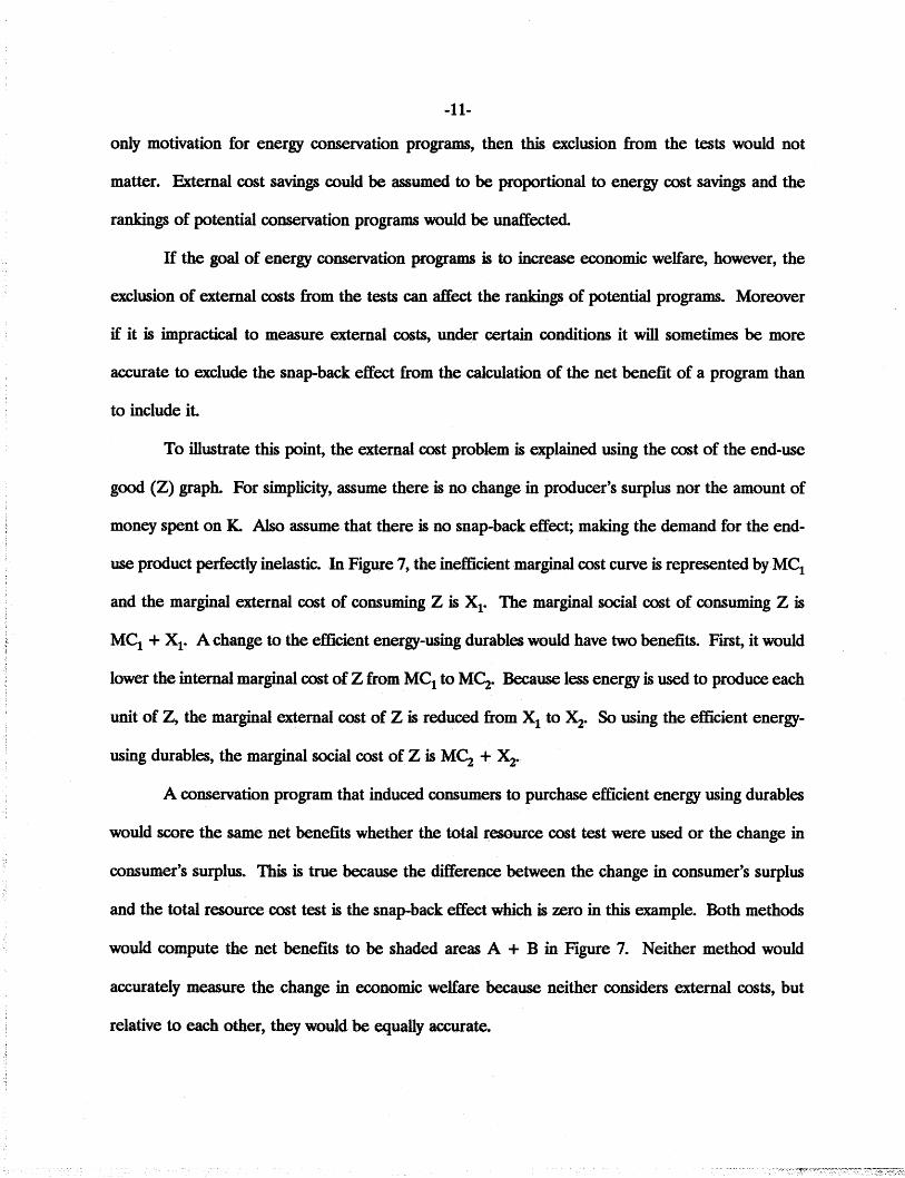
To illustrate this point, the external cost problem is explained using the cost of the end-use

good (Z) graph. For simplicity, assume there is no change in producer's surplus nor the amount of

money spent on K. Also assume that there is no snap-back effect; making the demand for the end­

use product perfectly inelastic. In Figure 7, the inemcientmarginal cost curve is represented byMCI

and the marginal external cost of consuming Z is Xl. The marginal social cost of consuming Z is

MCI + Xr A change to the efficient energy-using durables would have two benefits. First, it would

lower the internal marginal cost of Z from MClto M~.Becauseless energy is used to produce each

unit· of Z, the marginal external cost of Z is reduced from Xl to X2• So using the efficient energy­

using durables, the marginal social cost of Z is MC2 + X2•

A conservation program that induced consumers to purchase efficient energy using durables

would score the same net benefits whether the total resource cost test were used or the change in

consumer's surplus. This is true because the difference between the change in consumer's surplus

and the. total resource cost test is the snap-back effect which is zero in this example. Both methods

would compute the net·benefits ·to be shaded areas A + B in Figure 7. Neither method would

accurately measure the change in economic welfare because neither considers external costs, but

relative to each other,· they would be equally accurate.

$

N Figure 7et Benefit with . .and No S External Cost

nap-Back E~:uect

Z tEnd-Use Good)

-12-

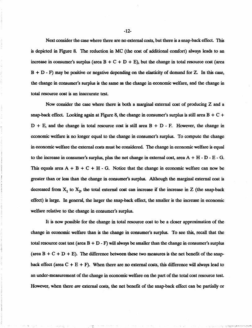
Next consider the case where there are no external costs, but there is a snap-back effect. This

is depicted in Figure 8. The reduction in Me (the cost of additional comfort) always leads to an

increase in consumer's surplus (area B + e + D + E), but the change in total resource cost (area

B + D - F) may be positive or negative dePending on the elasticity of demand for Z. In this case,

the change in consumer's surplus is the same as the change in economic welfare, and the change in

total resource cost is an inaccurate test.

Now consider the case where there is both a marginal external cost of producing Z and a

snap-back effect. Looking again at Figure 8, the change in consumer's surplus is still area B + e +

D + E, and the change in total resource cost is still area B + D - F. However, the change in

economic welfare is no longer equal to the change in consumer's surplus. To compute the change

in economic welfare the extemalcosts must be considered. The change in economic welfare is equal

to the increase in consumer's surplus, plus the net change in extemalcost, area A + H - D - E - G.

This equals area A + B· + e + H - G. Notice that the change in economic welfare can now be

greater than or less than the change·in consumer's surplus. Although the marginal external cost is

decreased from Xl to X2' the ·to181 external cost can increase if the increase in Z (the snap-back

effect) is large. In general, the larger the snap-back effect, the smaller is the increase in economic

welfare relative to the change in consumer's surplus.

It is now possible for the change in total resource cost to be a closer approximation of· the

change·in economic welfare than is the change in consumer's surplus. To see this, recall that the

total resource cost test (area B + D - F) will always be smaller than the change in consumer's surplus

(area B + e + D + E). The difference between these two measures is the net benefit of the snap­

back effect (area e + E + F). When there are noextemal costs, this difference win always lead to

an under-measurementof the change in economic welfare on the part of the total cost resource test.

However, when there are external costs, the net benefit of the snap-back effect can be partially or

Figure 8Net Benefit with External Cost

and a Snap-Back Effect

Z (End-Use Good)

-13-

entirely off-set by the change in total external costs, area A + H - D - E - G. If area D + E + G

is large relative to area A + H, then total external costs would increase. This condition will be true

when the snap-back effect (~ - Zl)· is large and when the initial and ending marginal external costs,

Xl and X2' are large.

The relevance of this result to the snap-back effect controversy is this: if the primary

motivation for energy conservation is the existence of large, but unmeasurable, external costs of

energy consumption, then the net benefits of the snap-back effect should not be included in the

calculation of costs and benefits. In other words, the total resource cost test would be a better

standard than the change in consumer's and producer's surplus. If, however, the primary motivation

for energy conservation is the apparent under-investment in efficient energy-using durables, then the

change -in consumer's and producer's surplus is a better standard than the total resource cost test.

-14­

REFERENCES

Berg, Sanford V. and John Tschirhart, Natural Monopoly Regulation: Principles and Practice,Cambridge University Press: Cambridge, 1988.

Burkhart, Lori A, "Conservation Program Cost-Benefit Analysis: Choosing Among Options," PublicUtilities Fortnightly, March 29, 1990, 41-44.

Cicchetti, Charles, Incentive Regulation: Some Conceptual and Policy Thoughts, Energy andEnvironmental Policy Center, Harvard University, June 1989.

Costello, Kenneth W., "Ten Myths of Energy Conservation," Public Utilities Fortnightly, March 19,1987, 19-22.

____-', andP. S. Galen, "An Approach·for Evaluating Utility-Financed Energy ConservationPrograms," Resources and Energy, 1985.

Einhorn, Michael A, "Measuring the Costs and Benefits of Conservation Programs," Public UtilitiesFortnightly, July 25, 1985, 22-26.

Florida· Public Service Commission, Cost Effectiveness Manual For Demand Side ManagementPrograms and Self Setvice Wheeling Proposals, September 4, 1990.

Hausman, Jerry A, "Individual Discount Rates and the Purchase and Utilization of Energy-UsingDurables," Bell Journal ofEconomics, Spring 1983, 33-54.

Hobbs, Benjamin F., "The Most Value Test: Economic Evaluation of Electricity Demand-SideManagement Considering Customer Value," The Energy Journal, Vol. 12, No.2, 1991, 67-91.

_____ and Sushil K. Nelson, "Assessing Conservation Payments: Least-Cost, Least-Rates, orMost-Value?," The Electricity Journal, July 1989, 28-39.

Just, Richard R, Darrell L. Hueth and Andrew Schmitz, Applied Welfare Economics and PublicPolicy, Prentice-Hall, Inc.: Englewood, NJ., 1982.

Khazzoom, J. D., "Economic· Implications of Mandated Efficiency Standards for HouseholdAppliances," The Energy Journal, October 1980, 21-40.

Lovins, A B., "Energy Saving Resulting from the Adoption of More Efficient Appliances: AnotherView," The Energy Journal, Vol. 9, No. 2, 1988, 155-62.

Norland, Douglas and James L. Wolf, "Utility Conservation Programs: A Regulatory and DesignFramework," Public Utilities Fortnightly, July 25, 1985, 15-21.

Sutherland, Ronald J., "Market Barriers to Energy Efficiency Investments," The Energy Journal, Vol.12, No.3, 1991, 15-34.