Abstract

Physical system behavior is continuous, but theuse of modeling abstractions to simplify systemdescription can result in behavior analysis on ahierarchy of time scales . At a given level ofdetail, behaviors on faster time scales are per-ceived to be instantaneous, therefore, the result-ing hybrid models encompass continuous behav-iors and discrete model configuration changes .These changes cause discontinuities in system be-havior generation which violate the physical prin-ciple of continuity of power, and sometimes causean instantaneous loss of energy in the system .This paper establishes a formal specification forhandling discrete model configuration changes atwell-defined points in time, and this allows for aconsistent transfer of the continuous system statefrom a previous model configuration to a new one .This is based on the principle of invariance ofstate . Simulation algorithms designed to oper-ate on hybrid models define behavior generationschemes that operate on the interval (continu-ous) to point (discrete) to interval (continuous)switches on the time line .

IntroductionPhysical systems are inherently continuous and theirbehaviors are governed by the principles of conserva-tion of energy and continuity of power [3] . Perceiveddiscontinuities are in reality nonlinear continuous be-haviors which operate at time scales much smallerthan the time scale of interest . For efficient analy-sis and behavior generation schemes, the differencesin time scale may be exploited so that the nonlinearbehaviors can be abstracted to manifest as ideal dis-continuities at points in time . An example is an idealelastic collision between a body and a floor where thevelocity of the body reverses instantaneously on im-pact . In reality, the collision takes a small time in-terval during which kinetic energy is converted intopotential elastic energy, which then reverts back com-pletely to kinetic energy for the body . Discontinuouseffects can also be created by parameter abstraction

Formal Specifications from Hybrid Bond Graph ModelsPieter J . Mosterman and Gautam Biswas

Center for Intelligent SystemsBox 1679, Sta B

Vanderbilt UniversityNashville, TN 37235.

pjm,biswasQvuse .vanderbi1t .edu[11] . Small parasitic physical effects that cause nonlin-ear continuous effects are abstracted away to simplifysystem description . For example, an ideal non-elasticcollision between two bodies involves instantaneousdiscontinuous changes in velocity for the two bodiesat the point of impact . A more precise model wouldhave included small elasticity coefficients for the twobodies, and the period of impact would be a small butfinite time interval, in which the change in velocitiesfor the bodies would occur in a continuous manner .Models that combine continuous and discrete effectsare called hybrid systems .During discontinuous changes, physical laws of con-

servation of energy and continuity of power may beviolated [11] . In such situations, the initial state vec-tor following the discontinuous changes is computedusing the principle of conservation of state along withexplicitly modeled interactions with the environment .In previous work [11, 13], this theory of discontinu-ous configuration changes in physical system modelshas been developed into a hybrid bond graph model-ing paradigm that combines traditional bond graphelements with ideal switching elements controlled byfinite state automata . Formal schemes for verifyingthe correctness of models based on the principle ofdivergence of time have also been developed [10, 13] .The hybrid bond graph formalism can be effectivelyapplied to systematically design and analyze hybridmodels of dynamic physical systems . This paper fo-cuses on developing a formal semantics for analyzingsystems with mixed continuous/discrete components .

A Hybrid Modeling ParadigmHybrid models operate in continuous modes (typicalphysical system behavior), but at points in time whensignal values cross pre-defined thresholds or when ex-plicit external (control) events are imposed on the sys-tem [14], changes in model configurations cause dis-crete changes in system behavior . An important ob-servation is that the temporal trajectory of systembehavior becomes piecewise continuous, where simplediscontinuities can occur only at well-defined pointsin time . The key to developing a correct modelingparadigm is to ensure that interaction between thecontinuous and discrete modeling formalisms is un-

Figure 1 : A general hybrid system .

ambiguous, rigorous, and consistent .

General Hybrid Dynamical SystemThe general architecture for a hybrid dynamical sys-tem model illustrated in Fig . 1 can be specified by the9-tuple [14] :

H=<I,E,0,X,U,f,,g,h,'Y>, (1)

Each mode of continuous behavior is given a uniquestate label ak E I . Continuous behavior is governedby field f,,,, which determines the continuous statevector x,,,, . The function h computes signal (s E S)values from the state vector xa ,, in mode ak, whichmay generate discrete events E specified by a mapping-y . y is usually defined in terms of signal values reach-ing or crossing pre-specified threshold values . Occur-rence of a discrete event suspends the continuous be-havior mode ak, and a new mode, ak+i, is generatedby the discrete transformation ¢ . The function g com-putes a new state vector, x+, for the new operationalmode ak+l using values of the continuous state vectorx ak in the previous operational mode ak .

The Continuous ModelDynamic physical system models are best representedas a set of differential equations on the system statevector . For example, the falling rod in Fig. 2 can bedescribed by three state variables, the rod's linear ve-locities, v= and vy , and its angular velocity, w . Whenit is falling freely, only gravity acts on the center ofmass and accelerates vertical movement . This can bedescribed by the differential equation

ca = 0, vy = 0, v y = ag ,

(2)

where ag is the gravitational acceleration .Differential equation state space models, supple-

mented by algebraic constraints (DAEs) directly re-flect underlying physical principles such as Kirchhoff'slaws and phenomenological relations like Ohm's law .Many model parameters have an immediate physical

132

meaning and equations can be systematically derivedfrom bond graphs, network representations, and blockdiagrams [2] . A general representation of an ODEmodel derived from DAEs is : i(t) = f,,(x(t), u(t), t) .The field, fQ, describes continuous temporal evolutionof system behavior in a mode of operation, a, withthe input vector, u, and the continuous state vector,x . Note that fa is unique in mode a.

The Discrete ModelDiscrete events are modeled by a discrete indexing set,I and a switching function, 0 : I x E -> I . The set ofdiscrete states corresponds to

" real modes, where system behavior is governedby energy principles, therefore, the state vectorchanges in time, and

" mythical modes [10, 13], where the system behav-ior transitions are instantaneous and state vectorchanges are used to infer real modes by ¢ .

E captures the event set . Events, o-, may be associ-ated with closed loop control, E� or they can be gov-erned by external, open loop, control signals, E_ (seeFig . 1) . (E = E, x Es .) The closed loop control is afunction of the system's physical process variables . 0,usually implemented with Petri-Nets or Finite StateAutomata, determines the next state after an eventoccurs .

InteractionsInteractions between the continuous and discretemodeling formalisms have to be specified correctly.For states that correspond to modes of continuous op-eration, ODES determine behavior . A discrete eventcauses the system to change operational mode, andthe correct state vector in the new mode is deter-mined by the function g : X x I -+ X+ . X definesstate vector values just before switching occurs, andX+ represents state vector values at the initial pointin time when a switch or mode change has occurred .A function h : X x U x I -+ S determines signalvalues S and S+, computed by h from X and X+,respectively. The function y : S x S+ -+ E, generatesdiscrete events from the signal values . The interactionbetween the continuous and discrete part consists of

" discrete events generated by the continuous signals,and

" a change of operational mode by the discrete model,requiring a consistent mapping of the continuousstate vector .

An example, adapted from [8], illustrates a rigidbody collision of a rod falling to the floor (Fig . 2) . Onhitting the floor, the rod may disconnect after a pointin time where contact occurred, slide along the floorand rotate about its point of contact, or just stick

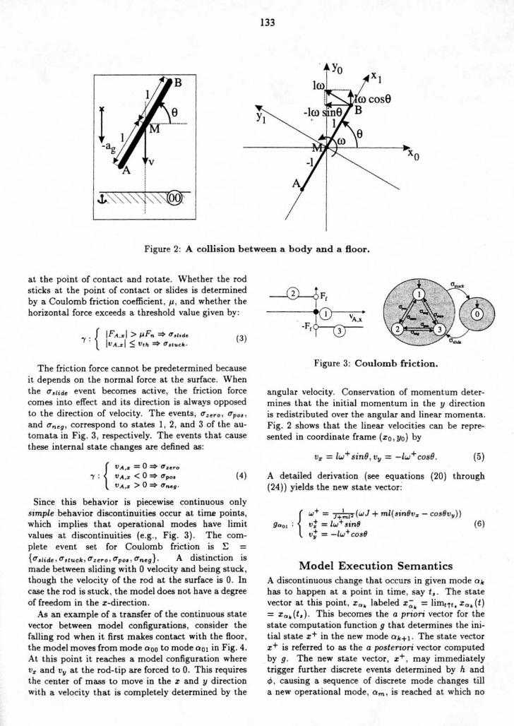
at the point of contact and rotate . Whether the rodsticks at the point of contact or slides is determinedby a Coulomb friction coefficient, u, and whether thehorizontal force exceeds a threshold value given by :

7:

IFA, .z l > PFn =* Q,l,de

'VA,xl < Vth -#' Qstuck .

VA,, = 0

Ozero

T :

VA,x < 0

Qpos

VA,x > 0

Cneg .

The friction force cannot be predetermined becauseit depends on the normal force at the surface . Whenthe Qslide event becomes active, the friction forcecomes into effect and its direction is always opposedto the direction of velocity . The events, Qzero, 17pos,and uneg, correspond to states 1, 2, and 3 of the au-tomata in Fig . 3, respectively . The events that causethese internal state changes are defined as :

Since this behavior is piecewise continuous onlysimple behavior discontinuities occur at time points,which implies that operational modes have limitvalues at discontinuities (e.g ., Fig . 3) . The com-plete event set for Coulomb friction is1 6 slide, Qstuck, Qzero, Qpos, cneg} .

A

distinction

ismade between sliding with 0 velocity and being stuck,though the velocity of the rod at the surface is 0 . Incase the rod is stuck, the model does not have a degreeof freedom in the x-direction .As an example of a transfer of the continuous state

vector between model configurations, consider thefalling rod when it first makes contact with the floor,the model moves from mode aoo to mode aol in Fig . 4 .At this point it reaches a model configuration wherev ., and vy at the rod-tip are forced to 0 . This requiresthe center of mass to move in the x and y directionwith a velocity that is completely determined by the

133

Figure 2 : A collision between a body and a floor .

9001

Figure 3 : Coulomb friction .

v,z = lw+ sinB, vy = -Iw+coso .

Model Execution Semantics

angular velocity . Conservation of momentum deter-mines that the initial momentum in the y directionis redistributed over the angular and linear momenta .Fig . 2 shows that the linear velocities can be repre-sented in coordinate frame (xo, yo) by

A detailed derivation (see equations (20) through(24)) yields the new state vector :

ml(singvx - cosOv,))v= = lw+sinB

(6)vy = -lw+cos9

A discontinuous change that occurs in given mode ak

has to happen at a point in time, say t, . The statevector at this point, x,,,, labeled xa k = limttt, x" k (t)= x,,, (t, ) . This becomes the a priori vector for thestate computation function g that determines the ini-tial state x+ in the new mode ak+i . The state vectorx+ is referred to as the a posteriori vector computedby g . The new state vector, x+, may immediatelytrigger further discrete events determined by h and6, causing a sequence of discrete mode changes tilla new operational mode, a,n , is reached at which no

Figure 4 : Operational modes of falling rod .

Figure 5 : System state is derived from the orig-inal state vector .

further switching occurs . All the intermediate statestraversed between two continuous modes are mythi-cal [10, 13] . The sequence of state and state vectorchanges is illustrated in Fig . 5 . At mode a�, systembehavior evolution in time resumes, with the state vec-tor x, m (t,) = x+ . Sometimes, mode a�, may repre-sent just a point of continuous operation (such as, thepoint of contact in an elastic collision [13]) . State vec-tor changes from x,,,(t .,) to x+ in the new real modemay cause the 7 function to generate additional eventsresulting in another sequence of discrete state changesbefore the next continuous operational mode, a� , isarrived at (see Fig . 5) .

Consider the falling rod in Fig . 4 . Initially, it isfalling freely under gravity (mode aoo) . On hittingthe floor it exerts a force with two components, FA, yand FA, (mode aoi) . Since the floor surface hasCoulomb friction, the rod immediately starts to slideif IFA,r l > MF� , mode all . Otherwise, it sticks and ro-tates around the point of contact (mode aoi) . Whenthe rod starts to slide, the floor exerts an opposingfriction force, Ff . In this case, the initial kinetic en-ergy before contact is redistributed over the angularand vertical momentum to ensure the vertical velocityof the rod-tip, VA,y , is 0 . The horizontal velocity oftherod-tip, VA,,, is determined by the angular velocity, w,and the horizontal velocity of the center of mass, vz .

134

Since vt is independent of w and determined by Ff, itis initially 0 and the discontinuous change of w resultsin a discontinuous change of VA, ., . Therefore, the sys-tem changes from the operational mode where Ff = 0to mode a2i where Ff = MF� .The grayed modes of operation in Fig . 4 are mythi-

cal . They do not have physical meaning, therefore, norepresentation on the real time-line . However, theyplay the role of transition points for locally definedswitching functions .

Temporal Evolution of State

Discontinuities are abrupt point changes, caused bymodeling abstractions . Discontinuities that persist intime intervals would violate continuity of power andconservation of energy principles . Further, asymme-try in temporal evolution ensures that the state vectorin modes of continuous operation has to be left closedover the time intervals these modes are active . Modechanges and discontinuous changes in the continuousstate vector can only occur at points in time t, . Wehave shown in other work [13] that further continu-ous evolution may cause a mode change, am to a� , atthe point of transfer, but no discontinuous change canoccur in the continuous state vector between xam (t,)and x+,, (t,) since its initial value would be derivedfrom lim t~t , x, � (t) which requires knowledge of futurebehavior and conflicts with the assumption of causal-ity in physical system models [14] .

Consider the stiction force when the rod discon-nects from the floor as it slides . If this force causesa discontinuous change in the vertical velocity of therod, lim t1t . vy (t) differs from the actual value vy (t,) .However, the value of limtj t , vy (t) may be such thatits value indicates that the rod would have gottenstuck . This implies that in addition to the current

state vy (t,) and model configuration, the operationalmode needs to know future modes and the limit valuesof state variables looking back in time . Such systemsare acausal which is physically impossible and resultsin ill-defined models .

Since no discontinuous change of the state vectorcan occur, it is continuous over a left closed intervalin time . This only requires the system state to operatecontinuously in left closed intervals but field f is notrequired to be differentiable . Therefore, other derivedsystem variables may still change discontinuously asa result of configuration changes . These jumps arewell-defined by the continuous state vector and modelconfiguration .

Invariance of StateA discontinuous change in the state vector may invokefurther mode transitions . The state vector in a newmode is computed from the last continuous state vec-tor, and the state vector in all new modes is computedfrom the last continuous state vector before switchingstarted . This is the principle of invariance of state[13] .To illustrate, consider the falling rod in Fig . 2 .

When it hits the floor, its vertical momentum is dis-tributed over its angular, horizontal and vertical mo-mentum to ensure its rotation and translation of cen-ter of mass are such that the point of contact doesnot move (mode aol ) . In this situation, if the force atthe rod-tip, FA ,,, exceeds a threshold value, it imme-diately starts to slide (mode all) . The rod-tip movesfreely in the x-direction, and its initial vertical mo-mentum is distributed only over its a posteriori angu-lar momentum and vertical momentum to ensure they-value does not change at the point of contact . Ifthe continuous state vector in the sliding mode, oil,was computed from the previously inferred mode, ooi,it would have a horizontal velocity associated with itscenter of mass which would keep the rod-tip from mov-ing in the x-direction as well, which is incorrect . Thisdemonstrates the importance of the proper computa-tion of the state vector across a series of discontinuouschanges .

Divergence of TimeDiscontinuous configuration changes in system behav-ior are instantaneous so a model verification tech-nique based on the principle of divergence of time en-sures that the model does not end up in a loop of in-stantaneous changes where system behavior does notprogress in time [13] . In previous work, we have de-veloped a multiple energy phase space analysis thatestablishes divergence of time before simulation is per-formed [11] .As an example, consider the falling rod when it

starts to slide because its force in the vertical direc-tion exceeds a threshold value . If the rod is specified

135

to stick when' the velocity of its rod-tip is below a cer-tain threshold value, it may not have sufficient initialvertical momentum to maintain a high enough verti-cal velocity . Based on the specifications, this movesthe model into the configuration where it sticks androtates around the point of contact . However, in thisconfiguration, based on the initial vertical momentum,its horizontal force causes it to start sliding and a loopof consecutive changes occurs .

Hybrid Bond Graph ModelingModeling of physical systems typically starts out withan ideal configurational representation from which aset of component equations is generated based on firstprinciples . As an intermediate step, a generic rep-resentation can be established to aid in a system-atic derivation of the set of equations . Depending onthe system configuration, the variables of these con-stituent equations are connected together, often in theform of a block diagram, and a number of mathemat-ical manipulation steps are performed to establish aset of explicit differential equations .

Bond GraphsTo support the modeling process, bond graphs [7] canbe used as a generic representation across domains interms of a small set of primitive elements with well-defined characteristics . Bond graphs are based on theobservation that all interaction in dynamic physicalsystems occurs by energy exchange, and, therefore,provides a unifying modeling approach across domains(e.g ., electrical, mechanical, chemical) . Energy ex-change is captured by its flow, or power, between el-ements . Power is the product of two conjugate vari-ables, e .g ., Power(P) = Voltage(V) x Current(I)in the electrical domain . In thermodynamics, thesevariables are distinguished as intensive and exten-sive variables, where intensive variables are definedat points and extensive variables are defined as anaggregate property over a region or volume [4] . Forexample, two bodies with the same velocity that areconnected together still have the same velocity butnow have twice the momentum. In bond graph terms,the intensive variables are referred to as efforts, e, andthe extensive variables as flows, f, e.g ., voltage andcurrent, pressure and volume flow .The basic bond graph elements are energy stor-

age, C and I, and energy dissipation, R, representingideal reversible and irreversible physical processes, re-spectively. These elements are connected by a junc-tion structure that consists of two basic types : (i) 0-junctions, the equivalent of electrical parallel connec-tions, that enforce common effort variables like volt-age and pressure, and (ii) 1-junctions, the equivalentof electrical series connections, that enforce commonflows like current and volume flow . The model con-text is specified by ideal sources of effort, Se, and flow,

Sf, that supply an effort or flow independent of theirload . If loading effects are important, they have tobe modeled by R, C, or I elements, and the contexthas become part of the model . The set of primitiveelements is completed by transformers, TF, and gyra-tors, GY . These elements are used to transform powerimpedance within and between physical domains .Based on this primitive set of nine elements, a wide

variety of systems can be modeled at different levelsof detail [5] . They rigorously specify f, X, U, and,therefore, capture the continuous model aspects un-ambiguously. The fundamental laws on which bondgraphs are based, conservation of energy and continu-ity of power [3], prohibit modeling of discontinuitiesin physical systems . Mosterman and Biswas [13] havebeen investigating the nature and effects of disconti-nuities in physical systems and established a theoryfrom which they derived the hybrid bond graph mod-eling paradigm [13] .

Hybrid Bond Graphs

Hybrid bond graphs rely on a local ideal switching el-ement to dynamically construct active model configu-rations . By introducing an ideal element, the conceptof reticulation on which bond graphs are based is notviolated, and non-ideal switching can be modeled byincluding ideal energy dissipating or storing elements .A higher level control structure forms a meta-modelthat controls the state of each of the ideal switchingelements . The meta-model is implemented as local fi-nite state automata, one associated with each switch .The switch becomes active when signal values in thecurrent bond graph configuration cross threshold val-ues . The system may transition through one or moreconfiguration changes before it arrives at a bond graphconfiguration where conservation of energy and conti-nuity of power governs system behavior again . Duringconfiguration changes these laws may be violated andmodel behavior is governed by the principle of invari-ance of state discussed earlier .

Local switches are implemented as controlled junc-tions . These junction can be

. on in which state they operate as normal junctions,and

off in which state they are deactivated .

To ensure correct loading, the deactivated junctionsare replaced by either 0 value effort sources or 0 valueflow sources, respectively (Fig . 6) . When turned off,they inhibit transfer of energy between model frag-ments that are connected through the junction . Afinite state automata associated with each controlledjunction interacts with the bond graph and determinesthe on/off state of the junctions based on events gen-erated by the bond graph, or from external controlevents .

136

Figure 6 : Operation of the controlled junction .

MSe: 0

MSe: FfMSe : -Ff

1sts~

Figure 7 : A multi-bond controlled junction tomodel Coulomb friction .

Piecewise continuous functions are represented ina compact form of the controlled junction by relyingon multi-bond notations [3] . For example, Coulombfriction in Fig . 3 in the hybrid bond graph frame-work is represented by the multi-bond representationin Fig . 7, where all source elements now are continu-ous functions over their active areas . This is requiredto make mode switches within source elements explicitin the hybrid bond graph framework . The net result isthis phenomena is easily incorporated into the mode-switching algorithm . This guarantees consistency inbehavior generation, since all discrete phenomena arehandled by one mechanism and all other influences arecontinuous .

Ideal switching behavior is established by enforcing0 effort or 0 flow [15] and by using signal values fromthe bond graph rather than power bonds to gener-ate discrete events . Controlled junctions in the bondgraph are marked with a subscript, e.g ., 01, 11, thatis used to identify the associated finite state machine .The signal values that are used by the finite state ma-chine to generate discrete events are shown as activebonds into the controlled junction (see Fig . 8), andspecify the h function . As the finite state automatarepresent a junction's control specification, they arereferred to as CSPECs. A CSPEC may contain se-quential logic with any number of internal states .However, each one of these has to map onto eithera junction's on or off state and, since each state re-flects a physical manifestation, on and off states haveto alternate in each transition sequence .

Local configuration changes may cause sequencesof consecutive configuration changes, and require thecontinuous state vector to be transferred correctly be-tween modes of continuous operation . When configu-ration changes occur, buffers may become dependentor modeled &sources may become active, which may

result in discontinuous change of the continuous statevector specified by g. Two cases exist : (1) one or morebuffers may become dependent on a source, or (ii) twoor more buffer elements become dependent on eachother or 6-sources become active, and the state vectorbetween the two configurations is different [10, 11] .In the first case, the energy stored in the dependentbuffers is determined by the value of the source, u,

P; = rs,iCiu,

where rs,i is the gain of the route from the source tothe dependent buffer, i, with value Ci . In the secondcase, the general formula

is the loss of generalized charge or momentum in thedependent buffers . The values of dependent states areprimed to

P+ = ro,iC,

P+

(10)i

Co o

which, along with (8) and (9), can be applied to deter-mine the new value of the independent state variable,PO+ . Note that if no b-sources become active, conser-vation of state holds because the amount of general-ized charge and momentum added to the independentbuffer equals the loss by each of the dependent bufferscombined . Therefore, the total amount of charge andmomentum in both modes remains the same . For ndependent buffers, buffer 0 is chosen in integral causal-ity and the new value of its stored energy, p+, is de-termined by

or [12],

PO = PO + ~(P; - pi) ri,o .

( 11)i--1

-

This can be expressed in terms of the value of theindependent buffer, po , by substituting (10)

CiPo = PO + ~(ro,iC

.PO - pi)ri,o

(12)i.1

n-1

n-1

PO+ (I -

ri,oro .i CC-,' ) =PO

-

ri,opi,

(13)i=1 ° i-1

where ri,o is the gain of the route from buffer i tobuffer 0 and Ci the buffer value of buffer i . Note thatthis may result in loss of energy to the environment[13] .

13 7

The meta-level control model separates discrete be-haviors as specified by the finite state automata andthe continuous state mapping function from the con-tinuous operation of the system where conservation ofenergy and continuity of power govern behavior . Aspart of the meta-model, a Mythical Mode Algorithm(MMA) is formulated to govern the global effects ofconfiguration changes [13] . The CSPEC conditionshave to be verified to always generate sequences ofconfiguration changes that terminate in a model con-figuration that has a real manifestation .

ImplementationThe bond graph model of the idealized thin rod andidealized floor, and the fragments dynamically gener-ated by simulation [12] are shown in Fig . 8 . The rodis assumed to have three degrees of freedom : angu-lar velocity, with a buffer element associated with theJ inertia, and linear velocity in the z and y direc-tions, with buffer elements mt and my , respectively .The relation between those velocities is derived ge-ometrically (Eq . (5)), and modeled by a modulatedtransformer . Gravity is modeled as a constant effortsource, may , in the y direction at the center of mass .

The x and y components of the forces and velocitiesat point A connect to the model at the Oc junction .If the body is moving freely, this junction is off. If thebody is in contact with the floor, Oc is on and if noother elements are connected, it enforces a 0 velocity .The friction force, Ff = uFn , in the x direction ismodeled as a piecewise continuous modulated source,MS,, producing force values 0, Ff , -Ff at A, oppositeto the direction of the surface velocity .The control specifications (CSPEC) of the switching

junctions are specified by finite state automata, onefor each controlled junction . The controlled junctionis is specified by a hierarchical finite state machine,which can be in one of several on states, dependingon the bond graph signals . Depending on the specificstate, a part of the piecewise continuous friction func-tion is active . In its off state, the junction enforces 0flow .

Initially, the rod is moving freely and controlledjunctions 0C and is are off. Replacing the junctionswith their 0 value sources results in the bond graph(mode aoo) shown in Fig . 8 . The position of the rod-tip closest to the floor, yA, is determined by the sumof the position of the center-point, yM = f vy , and thedistance of the rod-tip from the center point, -IsinO .If this position, xA = f vy -lsin8, becomes 0, the rodcollides with the floor and Oc comes on, and the modeltransitions to mode a01. This results in dependencybetween the linear and angular velocities, and the en-ergy redistribution that may be required, specified byg, is computed. If the rod-length and angle of colli-sion are such that is comes on (the model transitionsinto a11), the rod begins to slide . Based on the for-

PO = PO + E ad,iri,o + ab,j rj, o (8)buffers,i sources,]

can be applied, where

ab,i = Pi - Pi (9)

mulas for energy redistribution, the function, g, canbe calculated as before, and the piecewise continuousfriction function may move into its Ff area, mode a,>1 .

As shown by this example, the hybrid bond graph ap-proach provides a seamless integration of configura-tion changes based on local switches . Other examplesof hybrid bond graph models are discussed in [13] .

The continuous system model, directly derived fromeach operational mode of the hybrid bond graph(Fig . 8) is shown below (faoa is given in Eq . (2)) :

7 :

-mlcoaBW = Jagvs = lsin&~

' t by = -1t:OSBGJ-ml(coeB-yeinB).O _ JtmiFcoaB(coeB-yemB)ag

a2i =

vs = -N(lcos8~) +ag)v y = -1cos8w

Qoi

VA,, =0vA.s G 0V.4 .s > 0

ZeroQnegQpoa

(I4)

The discrete control model, 6, is specified by thetwo automata functions, C and S . The specificationfor the 7 and h functions are shown below .

138

Figure 8 : Dynamically generated models.

yq = f vydt - 1sinBvq,s = V s - lwsinB

pq,y = m(vy + lwcosB)

_ ~ 0

if aooFn -

m(vy -a g )

otherwise_ ~ 0

if aooFa,s -

mvs

otherwise

(16)

To derive g it is observed that in a hybrid bond graphdiscontinuous state changes only occur if buffers be-come dependent . Two cases exist :

1 . one or more buffers may become dependent on asource, and

2 . two or more buffer elements may become dependenton each other and b-sources become active . In thiscase, the state vector between the two configura-tions is different [11] .

In the first case, the a posteriors energy stored in thedependent buffers, pt, is determined by the value ofthe source, u (see equation r) . In the second case,Dirac pulses, J, are induced that enforce a discon-tinuous change of the independent, integrated, statevariable, po . The area of such a pulse combined withthe gain from its origin, either a source or dependentbuffer to the independent buffer, specifies a change ofP01 . This change is given by the general formula givenin equation 8 . The area adj is the explicitly modeledinteraction with the environment . The area a6,; can becalculated from equation 9, which is the loss of gener-alized charge or momentum in the dependent buffers .The new signals generated by dependent states, c,are forced to values determined by the new signal fromthe independent buffer, s , and the route gain from

4RSL-St :Ct Sf:o MSe--I 1 Se--I 10

9

ItrMTF~Se----1 1 Io m.

IF--MTF<0~F~1 F_I

m`0C~I 1~I I

1Fr-MTF<

in,0, -4 1 ~t I

IF~MTF m'-IsinaIcosa Se 1 -~t I J -lsina, 0~ 1 F~I [

-lsinaIcosa, 0, F~1 I~I J

[-IsinaIcon a, Oc F-' 1 F~I0 M, ]cosa

nil m

Se 01 Se 11 Se 21 Semag ma~ m a, m at,

tJA < 0 Apq.y < 0 QcontnctFn < () DJrceFA..' > FIFn n yA < 0 A pq,y < 0 QelidewA .s l <UthVFn <0 Qntuck

the independent buffer to the dependent one . This isdescribed by the equation 10, which along with equa-tion 8 and equation 9 can be applied to determine thenew value of the independent state variable, po .

In the special case that no explicitly modeled b-sources become active, conservation of state holds be-cause the amount of generalized charge and momen-tum added to the independent buffer equals the lossby each of the dependent buffers combined . Therefore,the total amount of charge and momentum in bothmodes remains the same . For n dependent buffers,buffer 0 is chosen in integral causality and the newvalue of its stored energy, po , is determined by

or [12],

So,

Po = PO +

(Pi - Pi )ri,oi--1

This can be expressed in terms of the value of theindependent buffer, po , by substituting Eq . (10)

n-1+

Ct +PO = PO + ~(ro,iCoPO _ pi)ri,o

i=1

n-1

n-1+ ~ C' _Po (1

ri,cro .j-o ) = Po

ri,opi,

(19)i=1

i-1

where ri,o is the gain of the route from buffer i tobuffer 0 and Ci the buffer value of buffer i . Note thatthis may result in loss of energy to the environment[13] .To demonstrate, we derive g,,,,,, . In the correspond-

ing operational mode, aol, there is dependency be-tween three buffers, J, rn, and my , with stored en-ergy hw , px, and p y , respectively. This represents thesituation where the center of mass moves with veloc-ity such that, in spite of the rotation around it, therod-tip A does not move in the horizontal or verticaldirection since it is in contact with the floor and stuck .Choosing J as the independent buffer, this results intwo dependent buffers, mx and my ,

Pm x - PT, Pi = rJ,fns

Itaa,+n v = Pm y - Py, Py = r,l,my

h+ .

(17)

(18)

(20)

buffers(21)

There are no b-sources active upon switching soSources = 0 . The complete expression for the in-

dependent energy, h+, now yieldsm

h~ = hw + rm,,JrJ,m,J hW - r+n-JPr +

139

event

find switchingdetected

time, i s

Figure 9 : Flow diagram of hybrid system simu-lation .

This can be transformed into the state variables bythe translations hw = Jw, Ps = mvr , and py = mvyand by substitution of the gains of the respectiveroutes, found by tracing power amplification along aroute following causal strokes (Fig . 8),

which yields

g :

aoo

a? 1

:

rmv,Jrj,mvfhW - rm y,JPy .(22)

occur at points in time.

rmr,J = -IsinO, rj,M== IsinO

rmy J = ICOSB, rj,,n y

-ICOSB,

w+ = wJ - MI(cosovy - sinOvz ) _

24j +m12()Analogously, the state vector mapping can be de-rived for the other operational modes (geo, is givenin Eq . (6))

vy = vy- wJ-MICOSOV

w - JJ+mc0828~Vs = vxvy = -1w+COS0w+ - wJ-m1(cos8-Nsin8)v ,

- J+m1 cos8(cos8-jjsin8)'Ui = -P(1w+ COSB + vy) + urvy = -Iw+Coso

(23)

(25)

In other work [13], we have used phase space analy-sis to verify the correctness of the model specifications,

_ (rj . .n= ~h+-px)rmi,J+(ri,m �~h+-Py)rmv,J i.e ., to ensure the given transition specifications willresult in the model behavior diverging in time, a prin-ciple that has to be satisfied by all physical systems .

Hybrid System SimulationThe simulator operates in two modes :

1 . continuous simulation in temporal intervals, and

2 . discrete instantaneous configuration changes that

The Simulation SchemeNumerical simulation schemes like Euler and Runge-Kutta can be used for continuous behavior modes.Discrete events generated by y trigger an event de-tection module to determine the switching time, t,,within a margin of tolerance, e (Fig . 9) . The contin-uous field, f« k , computes x, (t,), then real time issuspended, and the meta-level control model, 0, gen-erates the discrete state transition . The original con-tinuous state vector is then transferred to the newlyfound model configuration using g, and this may trig-ger further events . The resulting model configurationis established, and x ak (t,) is transferred to this modelconfiguration . Again, discrete events may be gener-ated and this process continues until no further tran-sitions occur and the prior continuous system state isupdated to x,,_(t,)

Further events are generated when the state vectoris updated and the a priori switching values change .This may cause a new series of configuration changesthat are executed by the discrete model using the dif-ferent h functions in each mode. There can be no morediscontinuous changes in the state vector . In the newcontinuous mode a� , fa � , defines the simulation fromtime t, with initial vector x,,,m (t,) (= x. � (t .,)) . Thisimplements simulation of f,,m at t, as a point in timeand allows an energy redistribution at a point spec-ified by a function with discontinuities that are notsimple. Note that the method only applies under theprinciple of temporal evolution of state .

Simulation of the Colliding RodTo derive a numerical model of the continuous func-

tion, f, a 0-order, forward Euler, approximation isused . A forward Euler approximation is obtained byusing i =

xkof

xk, or xk+1 = fAt -F- xk .

Deriva-tives that are part of expressions in f are replacedanalogously . For example, ily = lcosBw becomes

= 1(COJ8k+1Wk+1-COJBkWk~vs,k+1

At

_At +vs,k, Or, vs,k+1 =

lcosBk+1Wk+i - 1COSBkwk + vx,k = lcosBk+jWk+l . Theexpressions for 0k+i and YM,k+l are uniform acrossconfigurations . These equations combined with therest of the numerical model constitute the simulationof continuous behavior . The only other function ofthe analytical specification that has to be representedby a numerical equivalent is h :

YA = YM,k+l - 18inek+1

VA,x = "+,k+1 - 1sinok+1-k+t

PA,y = m(vy ,k+l +1c03Bk+1Wk+1)

Fn

0v

ifapp

(26)m( .",+I1 V

v.k- ay )

otherwise( 0

if aooFA .. =

V~k+1

vx,km xat

otherwise .

The rest of the specifications are not temporal andcan be directly used for simulation . Note that VA,x is

140

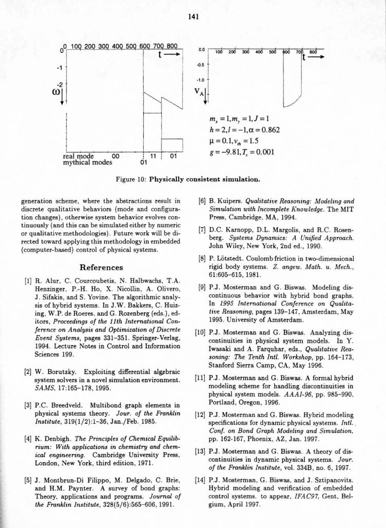
computed based on a posteriori values whereas PA,y(an energy variable) is computed from a priori values .A simulation run for one scenario is shown in

Fig . 10 . The rod falls down at a specific angle, hitsthe floor and moves into configuration aol . Based onthe state vector an immediate configuration change tomode all occurs . In this configuration the rod slideswith a velocity that decreases in magnitude due to thefriction force acting on the rod-tip . At one time, thisvelocity falls below a preset threshold value and if thestate vector is such that the rod gets stuck withoutimmediately satisfying the condition to slide, the sys-tem moves into mode aol . In this mode, it is stuckand rotates around the point of contact until it fallsflat on the floor .

ConclusionsThis work demonstrates a powerful hybrid systemmodeling scheme that incorporates modeling abstrac-tions and embedded discrete control of physical sys-tems . The modeling formalism, based on a hybridbond graph methodology, combines continuous bondgraph models with local discrete finite state automata .The automata define ideal switching specifications im-posed on bond graph junctions to create instantaneousmodel configuration changes . Configuration changesmay result in discontinuities in system variables . Thenew state variables are then systematically derivedusing the principle of conservation of state combinedwith explicitly defined interactions with the environ-ment . Global specifications are derived dynamicallybased on systematic principles of invariance of state,divergence of time, and temporal evolution of states .This simplifies the modeling task and truly demon-strates the use of compositionality in defining systemmodels . This is in contrast with the approach by Aluret al . [1] which requires pre-defined global specifica-tions of continuous system behavior in terms of dif-ferential equations . Furthermore, global knowledge inspecifying discrete behavior is required to ensure nomythical modes exist . Also, unlike the hybrid bondgraph modeling paradigm, there is no support for sys-tematic modeling based on physical principles (e.g .,conservation of state) . The formal specifications areincorporated into a hybrid system simulation schemethat ensures the generation of correct system behav-ior .

In the past, qualitative reasoning schemes have fo-cused on abstraction of the numerical properties ofsystem behavior variables [6] . This has often led tounderconstrained models resulting in an explosion ofpossible behaviors and the generation of physically in-consistent behaviors . Ours is a more systematic andencompassing approach to abstracting physical sys-tem models : (i) time scale abstraction, and (ii) ignor-ing parasitic parameter effects that often cause sharpnonlinearities . The result is a truly hybrid behavior

0 10 200 304 40Q 504 604 70Q 80Q

generation scheme, where the abstractions result indiscrete qualitative behaviors (mode and configura-tion changes), otherwise system behavior evolves con-tinuously (and this can be simulated either by numericor qualitative methodologies) . Future work will be di-rected toward applying this methodology in embedded(computer-based) control of physical systems .

References

R. Alur, C. Courcoubetis, N. Halbwachs, T.A .Henzinger, P.-H . Ho, X . Nicollin, A . Olivero,J . Sifakis, and S . Yovine . The algorithmic analy-sis of hybrid systems . In J.W . Bakkers, C. Huiz-ing, W.P. de Roeres, and G . Rozenberg (eds.), ed-itors, Proceedings of the 11th International Con-ference on Analysis and Optimization of DiscreteEvent Systems, pages 331-351 . Springer-Verlag,1994 . Lecture Notes in Control and InformationSciences 199 .

[2] W . Borutzky . Exploiting differential algebraicsystem solvers in a novel simulation environment .SAMS, 17 :165-178, 1995 .

P.C . Breedveld . Multibond graph elements inphysical systems theory . Jour. of the FranklinInstitute, 319(1/2) :1-36, Jan./Feb.,1985 .

[4] K . Denbigh . The Principles of Chemical Equilib-rium: With applications in chemistry and chem-ical engineering. Cambridge University Press,London, New York, third edition, 1971 .

J . Montbrun-Di Filippo, M. Delgado, C . Brie,and H.M . Paynter . A survey of bond graphs :Theory, applications and programs . Journal ofthe Franklin Institute, 328(5/6) :565-606, 1991 .

-0 .5

-1 .0

VAJ

Ms =1, m_,, =1,J =1

h=2,1=-1,a=0.862g =0.1, vth =1.5g=-9.81,T, =0.001

Figure 10 : Physically consistent simulation.

1

20

30,

40

50

70t

80

[6] B . Kuipers . Qualitative Reasoning : Modeling andSimulation with Incomplete Knowledge . The MITPress, Cambridge, MA, 1994 .

D .C . Karnopp, D.L . Margolis, and R.C . Rosen-berg . Systems Dynamics: A Unified Approach.John Wiley, New York, 2nd ed ., 1990 .

[8] P . Lotstedt . Coulomb friction in two-dimensionalrigid body systems . Z. angew . Math . u . Mech.,61 :605-615, 1981 .

P.J . Mosterman and G . Biswas . Modeling dis-continuous behavior with hybrid bond graphs .In 1995 International Conference on Qualita-tive Reasoning, pages 139-147, Amsterdam, May1995 . University of Amsterdam .

[10] P.J . Mosterman and G . Biswas . Analyzing dis-continuities in physical system models . In Y .Iwasaki and A. Farquhar, eds ., Qualitative Reasoning: The Tenth Intl . Workshop, pp . 164-173,Stanford Sierra Camp, CA, May 1996 .

[11] P.J . Mosterman and G . Biswas . A formal hybridmodeling scheme for handling discontinuities inphysical system models . AAAI-96, pp . 985-990,Portland, Oregon, 1996 .

[12] P.J . Mosterman and G . Biswas . Hybrid modelingspecifications for dynamic physical systems . Intl . ,Conf. on Bond Graph Modeling and Simulation,pp . 162-167, Phoenix, AZ, Jan . 1997 .

[13] P.J . Mosterman and G. Biswas . A theory of dis-continuities in dynamic physical systems . Jour.of the Franklin Institute, vol . 334B, no . 6, 1997 .

[14] P.J . Mosterman, G. Biswas, and J . Sztipanovits .Hybrid modeling and verification of embeddedcontrol systems . to appear, IFAC97, Gent, Bel-gium, April 1997 .

[15] Jan-Erik Stromberg, Jan Top, and Ulf Soderman .Variable causality in bond graphs caused by dis-crete effects . In Proceedings of the InternationalConference on Bond Graph Modeling, pages 115-119, San Diego, California, 1993.